a user’s guide to principal components - semantic scholar · a user's guide to principal...

A User’s Guide To Principal Components

J. EDWARD JACKSON

A Wiley-Interscience Publication JOHN WILEY & SONS, INC. New York Chichester Brisbane Toronto * Singapore

This Page Intentionally Left Blank


J. EDWARD JACKSON

A Wiley-Interscience Publication JOHN WILEY & SONS, INC. New York Chichester Brisbane Toronto * Singapore

A NOTE TO THE READER This book has been electronically reproduced from digital dormation stored at John Wiley & Sons, Inc. We are pleased that the use of this new technology will enable us to keep works of enduring scholarly value in print as long as there is a reasonable demand for them. The content of this book is identical to previous printings.

BMDP is a registered trademark of BMDP Statistical Software, Inc., Los Angeles, CA. LISREL is a registered trademark of Scientific Software, Inc., Mooresville, IN. SAS and SAS Views are registered trademarks of SAS Institute, Inc., Cary, NC. SPSS is a registered trademark of SPSS Inc., Chicago, IL.

In recognition of the importance of preserving what has been written, it is a policy of John Wiley & Sons, Inc., to have books of enduring value published in the United States printed on acid-free paper, and we exert our best efforts to that end.

Copyright 0 1991 by John Wiley & Sons, Inc.

All rights reserved. Published simultaneously in Canada.

No part of this publication may be reproduced, stored in a retrieval system or transmitted in any form or by any means, electronic, mechanical, photocopying, recording, scanning or otherwise, except as permitted under Sections 107 or 108 of the 1976 United States Copyright Act. without either the prior written permission of the Publisher, or authorization through payment of the appropriate per-copy fee to the Copyright Clearance Center, 222 Rosewood Drive, Danvers, MA 01923, (978) 750-8400, fax (978) 750-4470. Requests to the Publisher for permission should be addressed to the Permissions Department, John Wiley & Sons, Inc., 111 River Street, Hoboken, NJ 07030, (201) 748-601 1, fax (201) 748-6008, E-Mail: PERMREQOWILEY.COM.

To order books or for customer service please, call 1(800)-CALL-WILEY (225-5945).

Library of Congress Catabging in Publication Data:

Jackson. J. Edward. A user's guide to principal components / J. Edward Jackson.

cm. - (Wiley series in probability and mathematical p. statistics. Applied probability and statistics)

Includes bibliographical references and index. I. Principal components analysis. 1. Title. 11. Series.

QA278.5.J27 1991 519.5'354-dc20

ISBN 0-471-62267-2 90-28108 CIP

Printed in the United States of America

10 9 8 7 6 5 4 3 2

To my wife, Suzanne

Contents

Preface

Introduction

1. Getting Started

xv

1

4

1.1 Introduction, 4 1.2 A Hypothetical Example, 4 1.3 1.4 1.5 1.6 1.7

Characteristic Roots and Vectors, 7 The Method of Principal Components, 10 Some Properties of Principal Components, 13 Scaling of Characteristic Vectors, 16 Using Principal Components in Quality Control, 19

2. PCA With More Than Two Variables 26

2.1 2.2 2.3 2.4 2.5 2.6 2.1 2.8 2.9 2.10

Introduction, 26 Sequential Estimation of Principal Components, 27 Ballistic Missile Example, 28 Covariance Matrices of Less than Full Rank, 30 Characteristic Roots are Equal or Nearly So, 32 A Test for Equality of Roots, 33 Residual Analysis, 34 When to Stop?, 41 A Photographic Film Example, 51 Uses of PCA, 58

3. Scaling of Data 63

3.1 Introduction, 63 3.2

3.3

Data as Deviations from the Mean: Covariance Matrices, 64 Data in Standard Units: Correlation Matrices, 64

vii

viii CONTENTS

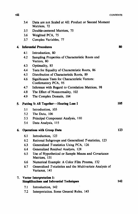
3.4 Data are not Scaled at All: Product or Second Moment Matrices, 72

3.5 Double-centered Matrices, 75 3.6 Weighted PCA, 75 3.7 Complex Variables, 77

4. Inferential Procedures

4.1 4.2

4.3 4.4 4.5 4.6

4.7 4.8 4.9

Introduction, 80 Sampling Properties of Characteristic Roots and Vectors, 80 Optimality, 85 Tests for Equality of Characteristic Roots, 86 Distribution of Characteristic Roots, 89 Significance Tests for Characteristic Vectors: Confirmatory PCA, 95 Inference with Regard to Correlation Matrices, 98 The Effect of Nonnormality, 102 The Complex Domain, 104

5. Putting It All Together-Hearing Loss I

5.1 Introduction, 105 5.2 The Data, 106 5.3 Principal Component Analysis, 110 5.4 Data Analysis, 115

6. Operations with Group Data

6.1 Introduction, 123 6.2 6.3 6.4 Generalized Residual Analysis, 128 6.5

6.6 6.7

Rational Subgroups and Generalized T-statistics, 123 Generalized T-statistics Using PCA, 126

Use of Hypothetical or Sample Means and Covariance Matrices, 131 Numerical Example: A Color Film Process, 132 Generalized T-statistics and the Multivariate Analysis of Variance, 141

7. Vector Interpretation I: Simplifications and Inferential Techniques

7.1 Introduction, 142 7.2 Interpretation. Some General Rules, 143

80

105

123

1 42

CONTENTS ix

7.3 Simplification, 144 7.4 7.5

Use of Confirmatory PCA, 148 Correlation of Vector Coefficients, 149

8. Vector Interpretation 11: Rotation

8.1 Introduction, 155 8.2 Simple Structure, 156 8.3 Simple Rotation, 157 8.4 Rotation Methods, 159 8.5 8.6 Procrustes Rotation, 167

Some Comments About Rotation, 165

9. A Case History-Hearing Loss I1

9.1 Introduction, 173 9.2 The Data, 174 9.3 Principal Component Analysis, 177 9.4 Allowance for Age, 178 9.5 Putting it all Together, 184 9.6 Analysis of Groups, 186

10. Singular Value Decomposition: Multidimensional Scaling I

10.1 10.2 10.3 10.4 10.5 10.6 10.7 10.8 10.9 10.10

Introduction, 189 R- and Q-analysis, 189 Singular Value Decomposition, 193 Introduction to Multidimensional Scaling, 196 Biplots, 199 MDPREF, 204 Point-Point Plots, 21 1 Correspondence Analysis, 214 Three-Way PCA, 230 N-Mode PCA, 232

11. Distance Models: Multidimensional Scaling I1

11.1 Similarity Models, 233 11.2 An Example, 234 11.3 Data Collection Techniques, 237 11.4 Enhanced MDS Scaling of Similarities, 239

155

173

189

233

X

12.

13.

14.

15.

CONTENTS

11.5 11.6 Scaling Individual Differences, 252 11.7 1 1.8

Do Horseshoes Bring Good Luck?, 250

External Analysis of Similarity Spaces, 257 Other Scaling Techniques, Including One-Dimensional Scales, 262

Linear Models I: Regression; PCA of Predictor Variables

12.1 Introduction, 263 12.2 Classical Least Squares, 264 12.3 Principal Components Regression, 271 12.4 12.5 Partial Least-Squares Regression, 282 12.6 Redundancy Analysis, 290 12.7 Summary, 298

Linear Models 11: Analysis of Variance; PCA of Response Variables

13.1 Introduction, 301 13.2 13.3 MANOVA, 303 13.4 13.5 Comparison of Methods, 308 13.6 13.7

Other Applications of PCA

14.1 Missing Data, 319 14.2 14.3 Tests for Multivariate Normality, 325 14.4 Variate Selection, 328 14.5 14.6 Time Series, 338

Methods Involving Multiple Responses, 28 1

Univariate Analysis of Variance, 302

Alternative MANOVA using PCA, 305

Extension to Other Designs, 309 An Application of PCA to Univariate ANOVA, 309

Using PCA to Improve Data Quality, 324

Discriminant Analysis and Cluster Analysis, 334

263

301

319

Flatland: Special Procedures for Two Dimensions 342

15.1 15.2

15.3 Correlation Matrices, 348 15.4 Reduced Major Axis, 348

Construction of a Probability Ellipse, 342 Inferential Procedures for the Orthogonal Regression Line, 344

CONTENTS

16. Odds and Ends

xi

350

16.1 16.2 16.3 16.4 16.5 16.6 16.7 16.8 16.9

Introdaction, 350 Generalized PCA, 350 Cross-validation, 353 Sensitivity, 356 Robust PCA, 365 g-Group PCA, 372 PCA When Data Are Functions, 376 PCA With Discrete Data, 381 [Odds and Ends]', 385

17. What is Factor Analysis Anyhow?

17.1 17.2 17.3 17.4 17.5 17.6 17.7 17.8 17.9 17.10

Introduction, 388 The Factor Analysis Model, 389 Estimation Methods, 398 Class I Estimation Procedures, 399 Class I1 Estimation Procedures, 402 Comparison of Estimation Procedures, 405 Factor Score Estimates, 407 Confirmatory Factor Analysis, 412 Other Factor Analysis Techniques, 416 Just What is Factor Analysis Anyhow?, 420

18. Other Competitors

18.1 Introduction, 424 18.2 Image Analysis, 425 18.3 Triangularization Methods, 427 18.4 Arbitrary Components, 430 18.5 Subsets of Variables, 430 18.6 Andrews' Function Plots, 432

Conclusion

Appendix A. Matrix Properties

424

435

437

A. 1 Introduction, 437 A.2 Definitions, 437 A.3 Operations with Matrices, 441

388

Appendix B. Matrix Algebra Associated with Principal Component Analysis 446

xii

Appendix C. Computational Methods

C.l Introduction, 450 C.2 C.3 The Power Method, 451 C.4 Higher-Level Techniques, 453 C.5 Computer Packages, 454

Solution of the Characteristic Equation, 450

Appendix D. A Directory of Symbols and Definitions for PCA

D.l Symbols, 456 D.2 Definitions, 459

Appendix E. Some Classic Examples

E. 1 Introduction, 460 E.2

E.3

Examples for which the Original Data are Available, 460 Covariance or Correlation Matrices Only, 462

Appendix F. Data Sets Used in This Book

F. 1 F.2 F.3 F.4 F.5 F.6 F.7 F.8 F.9 F.10 F.ll F.12 F.13 F.14 F.15 F.16 F.17 F.18 F.19 F.20

Introduction, 464 Chemical Example, 464 Grouped Chemical Example, 465 Ballistic Missile Example, 466 Black-and-white Film Example, 466 Color Film Example, 467 Color Print Example, 467 Seventh-Grade Tests, 468 Absorbence Curves, 468 Complex Variables Example, 468 Audiometric Example, 469 Audiometric Case History, 470 Rotation Demonstration, 470 Physical Measurements, 470 Rectangular Data Matrix, 470 Horseshoe Example, 471 Presidential Hopefuls, 471 Contingency Table Demo: Brand vs. Sex, 472 Contingency Table Demo: Brand vs. Age, 472 Three-Way Contingency Table, 472

CONTENTS

450

456

460

464

CONTENTS xiii

F.21 F.22 Linnerud Data, 473 F.23 Bivariate Nonnormal Distribution, 473 F.24 Circle Data, 473 F.25 United States Budget, 474

Occurrence ,of Personal Assault, 472

Appendix G. Tables

G.l G.2 G.3 G.4 G.5

G.6

Table of the Normal Distribution, 476 Table of the t-Distribution, 477 Table of the Chi-square Distribution, 478 Table of the F-Distribution, 480 Table of the Lawley-Hotelling Trace Statistic, 485 Tables of the Extreme Roots of a Covariance Matrix, 494

Bibliography

Author Index

475

497

551

563 Subject Index

Preface

Principal Component Analysis (PCA) is a multivariate technique in which a number of related variables are transformed to (hopefully, a smaller) set of uncorrelated variables. This book is designed for practitioners of PCA. It is, primarily, a “how-to-do-it” and secondarily a “why-it-works” book. The theoretical aspects of this technique have been adequately dealt with elsewhere and it will suffice to refer to these works where relevant. Similarly, this book will not become overinvolved in computational techniques. These techniques have also been dealt with adequately elsewhere. The user is focusing, primarily, on data reduction and interpretation. Lest one considers the computational aspects of PCA to be a “black box,” enough detail will be included in one of the appendices to leave the user with the feeling of being in control of his or her own destiny.

The method of principal components dates back to Karl Pearson in 1901, although the general procedure as we know it today had to wait for Harold Hotelling whose pioneering paper appeared in 1933. The development of the technique has been rather uneven in the ensuing years. There was a great deal of activity in the late 1930s and early 1940s. Things then subsided for a while until computers had been designed that made it possible to apply these techniques to reasonably sized problems. That done, the development activities surged ahead once more. However, this activity has been rather fragmented and it is the purpose of this book to draw all of this infarmation together into a usable guide for practitioners of multivariate data analysis. This book is also designed to be a sourcebook for principal components. Many times a specific technique may be described in detail with references being given to alternate or competing methods. Space considerations preclude describing them all and, in this way, those wishing to investigate a procedure in more detail will know where to find more information. Occasionally, a topic may be presented in what may seem to be less than favorable light. It will be included because it relates to a procedure which is widely used-for better or for worse. In these instances, it would seem better to include the topic with a discussion of the relative pros and cons rather than to ignore it completely.

As PCA forms only one part of multivariate analysis, there are probably few college courses devoted exclusively to this topic. However, if someone did teach a course about PCA, this book could be used because of the detailed development of methodology as well as the many numerical examples. Except for universities

xv

xvi PREFACE

with large statistics departments, this book might more likely find use as a supplementary text for multivariate courses. It may also be useful for departments of education, psychology, and business because of the supplementary material dealing with multidimensional scaling and factor analysis. There are no class problems included. Class problems generally consist of either theoretical proofs and identities, which is not a concern of this book, or problems involving data analysis. In the latter case, the instructor would be better off using data sets of his or her own choosing because it would facilitate interpretation and discussion of the problem.

This book had its genesis at the 1973 Fall Technical Conference in Milwaukee, a conference jointly sponsored by the Physical and Engineering Sciences Section of the American Statistical Association and the Chemistry Division of the American Society for Quality Control. That year the program committee wanted two tutorial sessions, one on principal components and the other on factor analysis. When approached to do one of these sessions, I agreed to do either one depending on who else they obtained. Apparently, they ran out of luck at that point because I ended up doing both of them. The end result was a series of papers published in the Journal of Quality Technology (Jackson, 1980, 1981a,b). A few years later, my employer offered an early retirement. When I mentioned to Fred Leone that I was considering taking it, he said, “Retire? What are you going to do, write a book?” I ended up not taking it but from that point on, writing a book seemed like a natural thing to do and the topic was obvious.

When I began my career with the Eastman Kodak Company in the late 194Os, most practitioners of multivariate techniques had the dual problem of performing the analysis on the limited computational facilities available at that time and of persuading their clients that multivariate techniques should be given any consideration at all. At Kodak, we were not immune to the first problem but we did have a more sympathetic audience with regard to the second, much of this due to some pioneering efforts on the part of Bob Morris, a chemist with great natural ability in both mathematics and statistics. It was my pleasure to have collaborated with Bob in some of the early development of operational techniques for principal components. Another chemist, Grant Wernimont, and I had adjoining offices when he was advocating the use of principal components in analytical chemistry in the late 1950s and I appreciated his enthusiasm and steady stream of operational “one-liners.” Terry Hearne and I worked together for nearly 15 years and collaborated on a number of projects that involved the use of PCA. Often these assignments required some special procedures that called for some ingenuity on our part; Chapter 9 is a typical example of our collaboration.

A large number of people have given me encouragement and assistance in the preparation of this book. In particular, I wish to thank Eastman Kodak’s Multivariate Development Committee, including Nancy Farden, Chuck Heckler, Maggie Krier, and John Huber, for their critical appraisal of much of the material in this book as well as some mainframe computational support for

PREFACE xvii

some of the multidimensional scaling and factor analysis procedures. Other people from Kodak who performed similar favors include Terry Hearne, Peter Franchuk, Peter Castro, Bill Novik, and John Twist. The format for Chapter 12 was largely the result of some suggestions by Gary Brauer. I received encouragement and assistance with some of the inferential aspects from Govind Mudholkar of the University of Rochester. One of the reviewers provided a number of helpful comments. Any errors that remain are my responsibility.

I also wish to acknowledge the support of my family. My wife Suzanne and my daughter Janice helped me with proofreading. (Our other daughter, Judy, managed to escape by living in Indiana.) My son, Jim, advised me on some of the finer aspects of computing and provided the book from which Table 10.7 was obtained (Leffingwell was a distant cousin.)

I wish to thank the authors, editors, and owners of copyright for permission to reproduce the following figures and tables: Figure 2.4 (Academic Press); Figures 1.1, 1.4, 1.5, 1.6, and 6.1 (American Society for Quality Control and Marcel Dekker); Figure 8.1 and Table 5.9 (American Society for Quality Control); Figures 6.3,6.4,6.5, and Table 7.4 (American Statistical Association); Figures 9.1, 9.2, 9.3, and 9.4 (Biometrie-Praximetrie); Figures 18.1 and 18.2 (Marcel Dekker); Figure 11.7 (Psychometrika and a. A. Klahr); Table 8.1 (University of Chicago Press); Table 12.1 (SAS Institute); Appendix G.1 (John Wiley and Sons, Inc.); Appendix G.2 (Biometrika Trustees, the Longman Group Ltd, the Literary Executor of the late Sir Ronald A. Fisher, F.R.S. and Dr. Frank Yates, F.R.S.); Appendices G.3, G.4, and G.6 (Biometrika Trustees); and Appen- dix G.5 (John Wiley and Sons, Inc., Biometrika Trustees and Marcel Dekker).

Rochester, New York January 1991

J. EDWARD JACKSON

Introduction

The method of principal components is primarily a data-analytic technique that obtains linear transformations of a group of correlated variables such that certain optimal conditions are achieved. The most important of these conditions is that the transformed variables are uncorrelated. It will be the purpose of this book to show why this technique is useful in statistical analysis and how it is carried out.

The first three chapters establish the properties and mechanics of principal component analysis (PCA). Chapter 4 considers the various inferential techniques required to conduct PCA and all of this is then put to work in Chapter 5, an example dealing with audiometric testing.

The next three chapters deal with grouped data and with various methods of interpreting the principal components. These tools are then employed in a case history, also dealing with audiometric examinations.

Multidimensional scaling is closely related to PCA, some techniques being common to both. Chapter 10 considers these with relation to preference, or dominance, scaling and, in so doing, introduces the concept of singular value decomposition. Chapter 1 1 deals with similarity scaling.

The application of PCA to linear models is examined in the next two chapters. Chapter 12 considers, primarily, the relationships among the predictor variables and introduces principal component regression along with some competitors. Principal component ANOVA is considered in Chapter 13.

Chapter 14 discusses a number of other applications of PCA, including missing data, data editing, tests for multivariate normality, discriminant and cluster analysis, and time series analysis. There are enough special procedures for the two-dimensional case that it merits Chapter 15 all to itself. Chapter 16 is a “catch-all” that contains a number of extensions of PCA including cross-validation, procedures for two or more samples, and robust estimation.

The reader will notice that several chapters deal with subgrouped data or situations dealing with two or more populations. Rather than devote a separate chapter to this, it seemed better to include these techniques where relevant. Chapter 6 considers the situation where data are subgrouped as one might find

1

2 INTRODUCTION

in quality control operations. The application of PCA in the analysis of variance is taken up in Chapter 13 where, again, the data may be divided into groups. In both of these chapters, the underlying assumption for these operations is that the variability is homogeneous among groups, as is customary in most ANOVA operations. To the extent that this is not the case, other procedures are called for. In Section 16.6, we will deal with the problem of testing whether or not the characteristic roots and vectors representing two or more populations are, in fact, the same. A similar problem is considered in a case study in Chapter 9 where some ad hoc techniques will be used to functionally relate these quantities to the various populations for which data are available.

There are some competitors for principal component analysis and these are discussed in the last two chapters. The most important of these competitors is factor analysis, which is sometimes confused with PCA. Factor analysis will be presented in Chapter 17, which will also contain a comparison of the two methods and a discussion about the confusion existing between them. A number of other techniques that may relevant for particular situations will be given in Chapter 18.

A basic knowledge of matrix algebra is essential for the understanding of this book. The operations commonly employed are given in Appendix A and a brief discussion of computing methods is found in Appendix C. You will find very few theorems in this book and only one proof. Most theorems will appear as statements presented where relevant. It seemed worthwhile, however, to list a number of basic properties of PCA in one place and this will be found in Appendix B. Appendix D deals with symbols and terminology-there being no standards for either in PCA. Appendix E describes a few classic data sets, located elsewhere, that one might wish to use in experimenting with some of the techniques described in this book. For the most part, the original sources contain the raw data. Appendix F summarizes all of the data sets employed in this book and the uses to which they were put. Appendix G contains tables related to the following distributions: normal, t, chi-square, F, the Lawley- Hotelling trace statistic and the extreme characteristic roots of a covariance matrix.

While the bibliography is quite extensive, it is by no means complete. Most of the citations relate to methodology and operations since that is the primary emphasis of the book. References pertaining to the theoretical aspects of PCA form a very small minority. As will be pointed out in Chapter 4, considerable effort has been expended elsewhere on studying the distributions associated with characteristic roots. We shall be content to summarize the results of this work and give some general references to which those interested may turn for more details. A similar policy holds with regard to computational techniques. The references dealing with applications are but a small sample of the large number of uses to which PCA has been put.

This book will follow the general custom of using Greek letters to denote population parameters and Latin letters for their sample estimates. Principal component analysis is employed, for the most part, as an exploratory data

INTRODUCTION 3

analysis technique, so that applications involve sample data sets and sample estimates obtained from them. Most of the presentation in this book will be within that context and for that reason population parameters will appear primarily in connection with inferential techniques, in particular in Chapter 4. It is comforting to know that the general PCA methodology is the same for populations as for samples.

Fortunately, many of the operations associated with PCA estimation are distribution free. When inferential procedures are employed, we shall generally assume that the population or populations from which the data were obtained have multivariate normal distributions. The problems associated with nonnormality will be discussed where relevant.

Widespread development and application of PCA techniques had to wait for the advent of the high-speed electronic computer and hence one usually thinks of PCA and other multivariate techniques in this vein. It is worth pointing out, however, that with the exception of a few examples where specific mainframe programs were used, the computations in this book were all performed on a 128K microcomputer. No one should be intimidated by PCA computations.

Many statistical computer packages contain a PCA procedure. However, these procedures, in general, cover some, but not all, of the first three chapters, in addition to some parts of Chapters 8 and 17 and in some cases parts of Chapters 10, 11, and 12. For the remaining techniques, the user will have to provide his or her own software. Generally, these techniques are relatively easy to program and one of the reasons for the many examples is to provide the reader some sample data with which to work. Do not be surprised if your answers do not agree to the last digit with those in the book. In addition to the usual problems of computational accuracy, the number of digits has often been reduced in presentation, either in this book or the original sources, to two or three digits for reason of space of clarity. If these results are then used in other computations, an additional amount of precision may be lost. The signs for the characteristic vectors may be reversed from the ones you obtain. This is either because of the algorithm employed or because someone reversed the signs deliberately for presentation. The interpretation will be the same either way.

C H A P T E R 1

Getting Started

1.1 INTRODUCTION

The field of multivariate analysis consists of those statistical techniques that consider two or more related random variables as a single entity and attempts to produce an overall result taking the relationship among the variables into account. A simple example of this is the correlation coefficient. Most inferential multivariate techniques are generalizations of classical univariate procedures. Corresponding to the univariate t-test is the multivariate 2''-test and there are multivariate analogs of such techniques as regression and the analysis of variance. The majority of most multivariate texts are devoted to such techniques and the multivariate distributions that support them.

There is, however, another class of techniques that is unique to the multivariate arena. The correlation coefficient is a case in point. Although these techniques may also be employed in statistical inference, the majority of their applications are as data-analytic techniques, in particular, techniques that seek to describe the multivariate structure of the data. Principal Component Analysis or PCA, the topic of this book, is just such a technique and while its main use is as a descriptive technique, we shall see that it may also be used in many inferential procedures as well.

In this chapter, the method of principal components will be illustrated by means of a small hypothetical two-variable example, allowing us to introduce the mechanics of PCA. In subsequent chapters, the method will be extended to the general case of p variables, some larger examples will be introduced, and we shall see where PCA fits into the realm of multivariate analysis.

1.2 A HYPOTHETICAL EXAMPLE

Suppose, for instance, one had a process in which a quality control test for the concentration of a chemical component in a solution was carried out by two different methods. It may be that one of the methods, say Method 1, was the

4

A HYPOTHETICAL EXAMPLE 5

standard procedure and that Method 2 was a proposed alternative, a procedure that was used as a back-up test or was employed for some other reason. It was assumed that the two methods were interchangeable and in order to check that assumption a series of 15 production samples was obtained, each of which was measured by both methods. These 15 pairs of observations are displayed in Table 1.1. (The choice of n = 15 pairs is merely for convenience in keeping the size of this example small; most quality control techniques would require more than this.)

What can one do with these data? The choices are almost endless. One possibility would be to compute the differences in the observed concentrations and test that the mean difference was zero, using the paired difference t-test based on the variability of the 15 differences. The analysis of variance technique would treat these data as a two-way ANOVA with methods and runs as factors. This would probably be a mixed model with methods being a fixed factor and runs generally assumed to be random. One would get the by-product of a run component of variability as well as an overall measure of inherent variability if the inherent variability of the two methods were the same. This assumption could be checked by a techniques such as the one due to Grubbs (1948, 1973) or that of Russell and Bradley (1958), which deal with heterogeneity of variance in two-way data arrays. Another complication could arise if the variability of the analyses was a function of level but a glance at the scattergram of the data shown in Figure 1.1 would seem to indicate that this is not the case.

Certainly, the preparation of Figure 1.1 is one of the first things to be considered, because in an example this small it would easily indicate any outliers or other aberrations in the data as well as provide a quick indication of the relationship between the two methods. Second, it would suggest the use of

Table 1.1. Data for Chemical Example

Obs. No. Method 1 Method 2

1 2 3 4 5 6 7 8 9

10 11 12 13 14 15

10.0 10.4 9.7 9.7

11.7 11.0 8.7 9.5

10.1 9.6

10.5 9.2

11.3 10.1 8.5

10.7 9.8

10.0 10.1 11.5 10.8 8.8 9.3 9.4 9.6

10.4 9.0

11.6 9.8 9.2

6 GETTING STARTED

12

I I

x x i

x * X

X X

X

7 8 9 10 I I 12 Method 1

FIGURE 1.1. Chemical example: original data. Reproduced from Jackson (1980) with permission of the American Society for Quality Control and Jackson ( 1985) with permission of Marcel Dekker.

regression to determine to what extent it is possible to predict the results of one method from the other. However, the requirement that these two methods should be interchangeable means being able to predict in either direction, which (by using ordinary least-squares) would result in two different equations. The least-squares equation for predicting Method 1 from Method 2 minimizes the variability in Method 1 given a specific level of Method 2, while the equation for predicting Method 2 from Method 1 minimizes the variability in Method 2 given a specific level of Method 1.

A single prediction equation is required that could be used in either direction. One could invert either of the two regression equations, but which one and what about the theoretical consequences of doing this? The line that will perform this role directly is called the orthogonal regression line which minimizes the deviations perpendicular to the line itseg This line is obtained by the method of principal components and, in fact, was the first application of PCA, going back to Karl Pearson (1901). We shall obtain this line in the next section and in so doing will find that PCA will furnish us with a great deal of other information as well. Although many of these properties may seem superiluous for this small two-variable example, its size will allow us to easily understand these properties and the operations required to use PCA. This will be helpful when we then go on to larger problems.

CHARACTERISTIC ROOTS AND VECTORS 7

In order to illustrate the method of PCA, we shall need to obtain the sample means, variances and the covariance between the two methods for the data in Table 1.1. Let xik be the test result for Method 1 for the kth run and the corresponding result for Method 2 be denoted by x Z k . The vector of sample means is %=[;:I=[ 10.00 ]

10.00

and the sample covariance matrix is

where s: is the variance and the covariance is

with the index of summation, k, going over the entire sample of n = 15. Although the correlation between x 1 and x 2 is not required, it may be of interest to estimate this quantity, which is

1.3 CHARACTERISTIC ROOTS AND VECTORS

The method of principal components is based on a key result from matrix algebra: A p x p symmetric, nonsingular matrix, such as the covariance matrix S, may be reduced to a diagonal matrix L by premultiplying and postmultiplying it by a particular orthonormal matrix U such that

U’SU = L (1.3.1)

The diagonal elements of L, Zl, 1 2 , . . . , I p are called the characteristic roots, latent roots or eigenualues of S . The columns of U, uI,u2, ..., up are called the characteristic oectors or eigenuectors of S. (Although the term latent vector is also correct, it often has a specialized meaning and it will not be used in this book except in that context.) The characteristic roots may be obtained from the solution of the following determinental equation, called the characteristic equation:

(1.3.2) 1s - lII = 0

8 GETTING STARTED

where I is the ideptity matrix. This equation produces a pth degree polynomial in 1 from which the values I , , 1 2 , . . . , lp are obtained.

For this example, there are p = 2 variables and hence,

.7986 - I .6793 = .124963 - 1.53291 + 1' =: 0

1.6793 .7343 - 1 1s - 111 '=

The values of 1 that satisfy this equation are I , = 1.4465 and l2 = .0864.

equations The characteristic vectors may then be obtained by the solution of the

[S - 1I]t, = 0 (1.3.3)

and

ti ui = - 4%

(1.3.4)

for i = 1, 2,. . . , p. For this example, for i = 1,

.7986 - 1.4465 [ .6793 [S - lJ]t1 =

These are two homogeneous linear equations in two unknowns. To solve, let t , , = 1 and use just the first equation:

-.6478 + .6793tz, = 0

The solution is tzl = .9538. These values are then placed in the normalizing equation (1.3.4) to obtain the first characteristic vector:

Similarly, using l2 = .0864 and letting tzz = 1, the second characteristic vector is

- .6902 u2 = [ .7236]

These characteristic vectors make up the matrix

1 .7236 -.6902 .6902 i .7236

u = [Ul j U2-J =

CHARACTERISTIC ROOTS AND VECTORS 9

which is orthonormal, that is,

u;u, = 1 u;uz = 1 u;uz = 0

Furthermore,

1 usu = .7236 0.6902][ .7986 .6793][ .7236 -.6902 [ -.6902 .7236 .6793 .7343 .6902 .7236

verifying equation (1.3.1). Geometrically, the procedure just described is nothing more than a principal

axis rotation of the original coordinate axes x1 and xz about their means as seen in Figures 1.2 and 1.3. The elements of the characteristic vectors are the direction cosines of the new axes related to the old. In Figure 1.2, u l l = .7236 is the cosine of the angle between the x,-axis and the first new axis; u2, = ,6902 is the cosine of the angle between this new axis and the x,-axis. The new axis related to u1 is the orthogonal regression line we were looking for. Figure 1.3 contains the same relationships for u2.

1 1 7 8 9 10 II 12

Method 1

FIGURE 1.2. Direction cosines for ul.

10

13

12-

I1

N 10

B 5 r" 9 -

8 -

7 -

GETTING STARTED

I I I I I

8,2 = 133.650 e22= 43.650

case,, - . a 0 2 = u,2

X

-

X

I I I I I

7 8 9 10 II 12

Except for p = 2 or p = 3, equation (1.3.2) is not used in practice as the determinental equations become unwieldy. Iterative procedures, described in Appendix C, are available for obtaining both the characteristic roots and vectors.

1.4 THE METHOD OF PRINCIPAL COMPONENTS

Now that all of the preliminaries are out of the way, we are now ready to discuss the method of principal components (Hotelling, 1933). The starting point for PCA is the sample covariance matrix S (or the correlation matrix as we shall see in Chapter 3). For a p-variable problem,

...

...

... where s: is the variance of the ith variable, x i , and slj is the covariance between the ith and jth variables. If the covariances are not equal to zero, it indicates that a linear relationship exists between these two variables, the

THE METHOD OF PRINCIPAL COMPONENTS 11

strength of that relationship being represented by the correlation coefficient,

The principal axis transformation obtained in Section 1.3 will transform p correlated variables xl, x2,. . . , x p into p new uncorrelated variables zl, z2,. . . , zp . The coordinate axes of these new variables are described by the characteristic vectors ui which make up the matrix U of direction cosines used in the transformation:

r i j = S i j / ( S i s j ) *

z = U [ X - %] (1.4.1)

Here x and R are p x 1 vectors of observations on the original variables and their means.

The transformed variables are called the principal components of x or pc’s for short. The ith principal component is

zi = u;cx - a3 (1.4.2)

and will have mean zero and variance I , , the ith characteristic root. To distinguish between the transformed variables and the transformed observations, the transformed variables will be called principal components and the individual transformed observations will be called z-scores. The use of the word score has its genesis in psychology and education, particularly in connection with factor analysis, the topic of Chapter 17. However, this term is now quite prevalent with regard to PCA as well, particularly with the advent of the mainframe computer statistical packages, so we will employ it here also. The distinction is made here with regard to z-scores because another normalization of these scores will be introduced in Section 1.6.

The first observation from the chemical data is

Substituting in (1.4.1) produces

z = [

so the z-scores for the first observation are z1 = .48 and z2 = .51. The variance of zl is equal to Il = 1.4465 and the variance of z2 is equal to 1, = .0864. As we shall see in Section 1.5.3, Il + I , are equal to the sum of the variances of the original variables. Table 1.2 includes, for the original 15 observations, the deviations from their means and their corresponding pc’s, z1 and z2 along with some other observations and quantities that will be described in Sections 1.6 and 1.7.

L

H

Tab

le 1

3 Ch

emic

al E

xam

ple.

Prio

eipa

l Com

pone

nts C

alcl

llatio

ns

1 2 3 4 5 6 7 8 9 10

11

12

13

14.

15

A

B C

D

-0

.4

- .3

- .3 1.7

1 .o

- 1.3

- .5 .1 - .4 .5

- .8

1.3 .1

- 1.5

.7

- .2 -0

.1 1.5 .8

- 1.2

- .7

- .6

- .4

.4

- 1.0

1.6

- .2

- .8

.48

.15

- .22

-.15

2.27

1.28

- 1.77

- -84

- .34

-.57

.64

- 1.27

2.04

- .07

- 1.64

.5 1

- .42

.2 1

.28

- .09

-.11 .03

-.16

-.so

-.01

- .06

-.17

.26

-.21

.46

.58

.18

- .26

-.18

2.72

1.53

-213

- 1.02

-.41

- .68

.77

- 1.53

2.46

- .08

- 1.97

.15

-.12

.06

-08

- .03

- .03

.01

- .05

-.15

- .oo

- .02

- -0

5 .08

- .06

.13

.40

.13

-.18

-.12

1.88

1.06

- 1.47

- .70

- .28

- .47

.53

- 1.06

1.70

- .05

- 1.36

1.72

- 1-43

.70

.95

- .30

- .38

so

- .55

- 1.71

- .05

-A9

- .58

.89

- .73

1.55

3.12

2.06

.52

.92

3.62

1.27

2.17

.79

3.00

.22

.32

1.46

3.68

.54

4.25

23

2.5

3.39

-22

4.08

-07

2.82

.75

8.5 1

- 3.0

- 27

-4.03

.12

-4.85

.03

- 3.35

.40

11.38

1 .o

- 1.0

.03

- 1.41

.04

- .42

.03

-4.81

23.14

- 2.7

- .9

- 2.57

1.21

-3.10

.36

-2.14

4.12

21.55

Var

ianc

e

obse

rvat

ions

-

for

.7986

.7343

1.4465

.0864

2.0924

.0075

1 .o

1 .o

1-15

s: 4

4 12

1:

1: - -

- - - -

- -

- -

-

SOME PROPERTIES OF PRINCIPAL COMPONENTS 13

1.5 SOME PROPERTIES OF PRINCIPAL COMPONENTS

1.5.1 Transformations

If one wishes to transform a set of variables x by a linear transformation z = U[x - %] whether U is orthonormal or not, the covariance matrix of the new variables, S,, can be determined directly from the covariance matrix of the original observations, S, by the relationship

s, = U’SU (1.5.1)

However, the fact that U is orthonormal is not a sufficient condition for the transformed variables to be uncorrelated. Only this characteristic vector solution will produce an S, that is a diagonal matrix like L producing new variables that are uncorrelated.

15.2 Interpretation of Principal Components

The coefficients of the first vector, .7236 and .6902, are nearly equal and both positive, indicating that the first pc, zl, is a weighted average of both variables. This is related to variability that x1 and x2 have in common; in the absence of correlated errors of measurement, this would be assumed to represent process variability. We have already seen that u1 defines the orthogonal regression line that Pearson (1901) referred to as the “line of best fit.” The coefficients for the second vector, - ,6902 and .7236 are also nearly equal except for sign and hence the second pc, z2, represents differences in the measurements for the two methods that would probably represent testing and measurement variability. (The axis defined by u2 was referred to by Pearson as the “line of worst fit.” However, this term is appropriate for the characteristic vector corresponding to the smallest characteristic root, not the second unless there are only two as is the case here.)

While interpretation of two-variable examples is quite straightforward, this will not necessarily be the case for a larger number of variables. We will have many examples in this book, some dealing with over a dozen variables. Special problems of interpretation will be taken up in Chapters 7 and 8.

1.5.3 Generalized Measures and Components of Variability

In keeping with the goal of multivariate analysis of summarizing results with as few numbers as possible, there are two single-number quantities for measuring the overall variability of a set of multivariate data. These are

1. The determinant of the covariance matrix, IS I. This is called the generalized variance. The square root of this quantity is proportional to the area or volume generated by a set of data.

14 GETTING STARTED

2. The sum of the variances of the variables:

s: + si + + s l = Tr(S) (The trace of S)

Conceivably, there are other measures of generalized variability that may have certain desirable properties but these two are the ones that have found general acceptance among practitioners.

A useful property of PCA is that the variability as specified by either measure is preserved.

1. IS1 = ILI = I , I 2.. I , (1.5.2)

that is, the determinant of the original covariance matrix is equal to the product of the characteristic roots. For this example,

2. Tr(S) = Tr(L) (1.5.3)

that is, the sum of the original variances is equal to the sum of the characteristic roots. For this example,

S: + S; = .7986 + .7343 = 1.5329

= 1.4465 + .0864 = I , + l2 The second identity is particularly useful because it shows that the character-

istic roots, which are the variances of the principal components, may be treated as variance components. The ratio of each characteristic root to the total will indicate the proportion of the total variability accounted for by each pc. For zl, 1.4465/1.5329 = .944 and for z2, .0864/1.5329 = .056. This says that roughly 94% of the total variability of these chemical data (as represented by Tr(S) is associated with, accounted for or “explained by” the variability of the process and 6% is due to the variability related to testing and measurement. Since the characteristic roots are sample estimates, these proportions are also sample estimates.

1.5.4 Correlation of Principal Components and Original Variables

It is also possible to determine the correlation of each pc with each of the original variables, which may be useful for diagnostic purposes. The correlation of the ith pc, z,, and the jth original variable, xi, is equal to

(1.5.4)

SOME PROPERTIES OF PRINCIPAL COMPONENTS 15

For instance, the correlation between z1 and x1 is

and the correlations for this example become

z1 z2 .974 -.227 :: [.969 .248]

The first pc is more highly correlated with the original variables than the second. This is to be expected because the first pc accounts for more variability than the second. Note that the sum of squares of each row is equal to 1.0.

1.5.5 Inversion of the Principal Component Model

Another interesting property of PCA is the fact that equation (1.4.1),

2 = U [ X - j z ]

may be inverted so that the original variables may be stated as a function of the principal components, viz.,

x = j z + u z (1.5.5)

because U is orthonormal and hence U-' = U . This means that, given the z-scores, the values of the original variables may be uniquely determined.

Corresponding to the first observation, the z-scores, .48 and 3, when substituted into ( 1.5.5), produce the following:

.7236 -.6902 .48 [ = [ + [ .6902 .7236][ .51]

Said another way, each variable is made up of a linear combination of the pc's. In the case of x1 for the first observation,

x1 = 21 + U l l Z 1 + U12ZZ

= 10.0 + (.7236)(.48) + (-.6902)(.51) = 10.0

This property might seem to be of mild interest; its true worth will become apparent in Chapter 2.

16 GETTING STARTED

1.5.6 Operations with Population Values

As mentioned in the Introduction, nearly all of the operations in this book deal with sample estimates. If the population covariance matrix, C, were known, the operations described in this chapter would be exactly the same. The characteristic roots of X would be noted by A l , A, , . . . ,A, and would be population values. The associated vectors would also be population values. This situation is unlikely in practice but it is comforting to know that the basic PCA procedure would be the same.

1.6 SCALING OF CHARACTERISTIC VECTORS

There are two ways of scaling principal components, one by rescaling the original variables, which will be discussed in Chapter 3, and the other by rescaling the characteristic vectors, the subject of this section.

The characteristic vectors employed so far, the U-vectors, are orthonormal; they are orthogonal and have unit length. These vectors are scaled to unity. Using these vectors to obtain principal components will produce pc’s that are uncorrelated and have variances equal to the corresponding characteristic roots.

There are a number of alternative ways to scale these vectors. Two that have found widespread use are

vi = (i.e., v = ~ ~ 1 ’ 2 ) (1.6.1)

wi = ui/& (i-e., w = ~ ~ - 1 ’ 2 ) (1.6.2)

Recalling, for the chemical example, that

= [ .7236 -.6902] .6902 .7236

with I, = 1.4465 and I , = .0864, these transformations will produce:

1 .8703 -.2029 V = [

.8301 ,2127

= [ .6016 -2.34811 .5739 2.4617

For transformation ( 1.6.1 ), the following identities hold:

V’V = L (1.6.3)

.8703 -.2029] - - [ 1.4465 0 ] [ -:;::: :::::I[ .8301 .2127 0 .0864

SCALING OF CHARACTERISTIC VECTORS 17

VV’ = s (1.6.4)

[ .8703 - .2029][ .8703 .8301] - - [ .7986 .6793] .8301 .2127 -.2029 .2127 .6793 .7343

Although V-vectors are quite commonly employed in PCA, this use is usually related to model building and specification. The scores related to (1.6.6) are rarely used and hence we will not waste one of our precious symbols on it.

Corresponding to (1.3.1), there is

V’SV = L2 (1.6.5)

] = [ 2*or .175]

Recalling that L is a diagonal matrix, equation (1.6.3) indicates that the V-vectors are still orthogonal but no longer of unit length. These vectors are scaled to their roots. Equation (1.6.4) shows that the covariance matrix can be obtained directly from its characteristic vectors. Scaling principal components using V-vectors, viz.,

&z, = v;cx - a] (1.6.6)

may be useful because the principal components will be in the same units as the original variables. If, for instance, our chemical data were in grams per liter, both of these pc’s and the coefficients of the V-vectors themselves would be in grams per liter. The variances of these components, as seen from (1.6.5) are equal to the squares of the characteristic roots. The pc’s using (1.6.6) for the chemical data are also shown in Table 1.2.

Regarding now the W-vectors as defined in (1.6.2),

W’W = L-1 (1.6.7)

[ .6016 .5739][ .6016 -2.34811 - - [.6913

0 ] -2.3481 2.4617 .5739 2.4617 0 11.5741

W‘SW = I (1.6.8)

.6016 .5739][ .7986 .6793][ .6016 -2.34811 = [ 1 O] [ -2.3481 2.4617 .6793 .7343 .5739 2.4617 0 1

Equation ( 1.6.8) shows that principal components obtained by the transformation

y, = w;cx - f] ( 1.6.9)

18 GETTING STARTED

will produce pc’s that are still uncorrelated but now have variances equal to unity. Values of this quantity are called y-scores. Since pc’s are generally regarded as “artificial” variables, scores having unit variances are quite popular for data analysis and quality control applications; y-scores will be employed a great deal in this book. The relation between y- and z-scores is

zi = J X Y i (1.6.10) Zi

yi=Jil The W-vectors, like U and V, are also orthogonal but are scaled to the reciprocal of their characteristic roots. The y-scores for the chemical data are also shown in Table 1.2.

Another useful property of W-vectors is

ww’ = s-‘ (1.6.11)

[ .6016 -2.3481][ .6016 .5739] = [ 5.8755 -5.43511 .5739 2.4617 -2.3481 2.4617 - 5.4351 6.3893

This means that if all of the characteristic vectors of a matrix have been obtained, it is possible to obtain the inverse of that matrix directly, although one would not ordinarily obtain it by that method. However, in the case of covariance matrices with highly correlated variables, one might obtain the inverse with better precision using ( 1.6.1 1 ) than with conventional inversion techniques.

There are other criteria for normalization. Jeffers ( 1967), for instance, divided each element within a vector by its largest element (like the t-vectors in Section 1.3) so that the maximum element in each vector would be 1.0 and all the rest would be relative to it.

One of the difficulties in reading the literature on PCA is that there is no uniformity in notation in general, and in scaling in particular. Appendix D includes a table of symbols and terms used by a number of authors for both the characteristic roots and vectors and the principal components resulting from them.

In summary, with regard to scaling of characteristic vectors, principal components can be expressed by (1.4.1), (1.6.6), or (1.6.9). The three differ only by a scale factor and hence the choice is purely a matter of taste. U-vectors are useful from a diagnostic point of view since the vectors are scaled to unity and hence the coefficients of these vectors will always be in the range of zk 1 regardless of the original units of the variables. Significance tests often involve vectors scaled in this manner. V-vectors have the advantage that they and their corresponding pc’s are expressed in the units of the original variables. W-vectors produce pc’s with unit variance.

USING PRINCIPAL COMPONENTS IN QUALITY CONTROL 19

1.7 USING PRINCIPAL COMPONENTS IN QUALITY CONTROL

1.7.1 Principal Components Control Charts

As will be seen elsewhere in this book, particularly in Chapters 6 and 9, PCA can be extremely useful in quality control applications because it allows one to transform a set of correlated variables to a new set of uncorrelated variables that may be easier to monitor with control charts. In this section, these same principles will be applied to the chemical data. These data have already been displayed, first in their original form in Table 1.1 and then in terms of deviations from their means in Table 1.2. Also included in Table 1.2 are the scores for the three scalings of the principal components discussed in the previous section and an overall measure of variability, T2, which will be introduced in Section 1.7.4. Table 1.2 also includes four additional points that have not been included in the derivations of the characteristic vectors but have been included here to exhibit some abnormal behavior. These observations are:

Point x1 X2

A 12.3 12.5 B 7.0 7.3 C 11.0 9.0 D 7.3 9.1

Figure 1.4 shows control charts both for the original observations, x1 and x2 and for the y-scores. All four of these charts have 95% limits based on the variability of the original 15 observations. These limits will all be equal to the standard deviations of the specific variables multiplied by 2.145, that value of the t-distribution for 14 degrees of freedom which cuts off .025 in each tail. (When controlling with individual observations rather than averages, 95% limits are often used rather than the more customary “three-sigma” limits in order to reduce the Type I1 error.)

Common practice is to place control limits about an established standard for each of the variables. In the absence of a standard, as is the case here, the sample mean for the base period is substituted. This implies that we wish to detect significant departures from the level of the base period based on the variability of that same period of time.

For these four control charts, these limits are:

xi:

x2:

10.00 f,(2.145)(.89) = 8.09, 11.91

10.00 f (2.145)(.86) = 8.16, 11.84

y, andy,: 0 f (2.145)( 1) = -2.145, 2.145

GETTINO STARTED

. 1 1 l 1 1 1 1 1 1 1 1 1 1 1 1 l l * l

I 3 5 7 9 II 13 IS A B C O

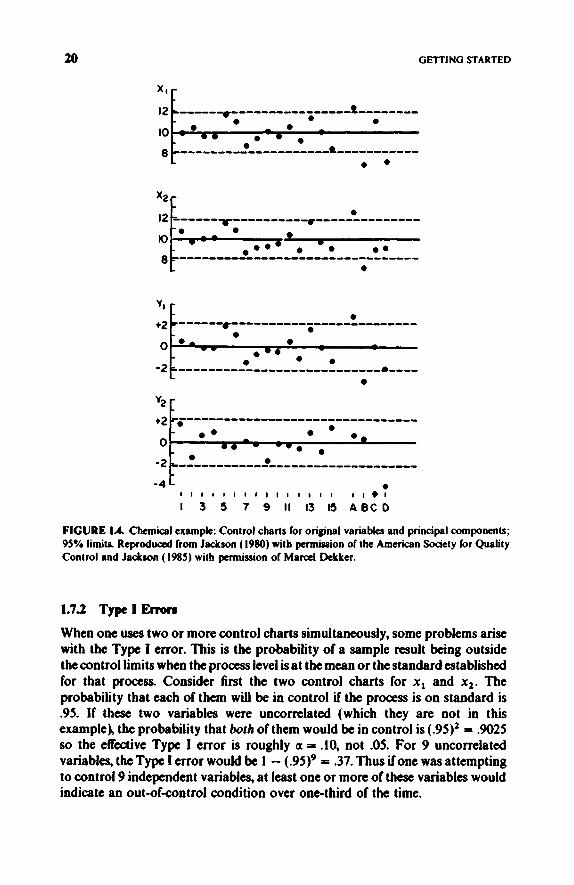
FIGURE 1.4. Chemical example: Control charts for original variabks and principal components; 95% limits. Reproduced from Jackson (1980) with permission of the American Society for Quality Control and Jackson (1985) with permission of Marcel Dekker.

-4 t

1.7.2 TypcIErrors

When one uses two or more control charts simultaneously, some problems arise with the Type I error. This is the probability of a sample result being outside the control limits when the process level is at the mean or the standard established for that process. Consider first the two control charts for x1 and x2. The probability that each of them will be in control if the process is on standard is .95. If these two variables were uncomlated (which they are not in this example), the probability that both of them would be in control is (.9S)2 = 9025 so the effkctive Type I error is roughly a = .lo, not .05. For 9 uncomlated variables, the Type I error would be 1 - (.95)9 = .37. Thus if one was attempting to control 9 independent variables, at least one or more of these variables would indicate an out-ofcontrol condition over one-third of the time.


The problem becomes more complicated when the variables are correlated as they are here. If they were perfectly correlated, the Type I error would remain at .05. However, anything less than that, such as in the present example, would leave one with some rather involved computations to find out what the Type I error really was. The use of principal component control charts resolved some of this problem because the pc’s are uncorrelated; hence, the Type I error may be computed directly. This may still leave one with a sinking feeling about looking for trouble that does not exist.

One possible solution would be to use Bonferroni bounds (Seber, 1984, p. 12 and Table D.l), which is a method of opening up the limits to get the desired Type I error. The limits for each variable would have a significance level of alp or, for this example, .05/2 = .025. These are conservative bounds yielding a Type I error of at most a. For the Chemical example, the limits would be increased from f2.145~~ to +2.510si for the original variables and would be k2.510 for the y-scores. These bounds would handle the Type I error problem for pc control charts but not for any situation where the variables are correlated.

1.7.3 Goals of Multivariate Quality Control

Any multivariate quality control procedure, whether or not PCA is employed, should fulfill four conditions:

1. A single answer should be available to answer the question: “Is the process

2. An overall Type I error should be specified. 3. The procedure should take into account the relationships among the

4. Procedures should be available to answer the question: “If the process is

in control?”

variables.

out-of-control, what is the problem?”

Condition 4 is much more difficult than the other three, particularly as the number of variables increases. There usually is no easy answer to this, although the use of PCA may help. The other three conditions are much more straightforward. First, let us consider Condition 1.

1.7.4 An Overall Measure of Variability: T2

The quantity shown in Figure 1.5

T2 = y‘y (1.7.1)

is a quantity indicating the overall conformance of an individual observation vector to its mean or an established standard. This quantity, due to Hotelling, (1931), is a multivariate generalization of the Student t-test and does give a single answer to the question: “Is the process in control?”

22

*::I 15.0

0

GETTING STARTED

4.0

0 0

0 0

0 1 1 9 1 I I I 1 1 0 . 1 1 ? 1 I I I I

I 3 5 7 9 II 13 15 A B C D

FIGURE IS. Chemical example: T2-chart; 95% limits. Reproduced from Jackson (1980) with permission of the American Society for Quality Control and Jackson (1985) with permission of Marcel Dekker.

The original form of T 2 is

T2 = [X - %]'S-'[X - 23 (1.7.2)

which does not use PCA and is a statistic often used in multivariate quality control. From (1.6.11), S-' = WW'. Substituting in (1.7.2) and using (l.6.9),

T2 = [X - %]'S-'[X - %]

= [x - jz]'WW'[X - j z ] = y'y (1.7.3)

so (1.7.1) and (1.7.2) are equivalent. The important thing about T 2 is that it not only fulfills Condition 1 for a proper multivariate quality control procedure but Conditions 2 and 3 as well. The only advantage of (1.7.1) over (1.7.2) is that if W has been obtained, the computations are considerably easier as there is no matrix to invert. In fact, y'y is merely the sum of squares of the principal components scaled in this manner ( T 2 = y: + y : for the two-variable case) and demonstrates another advantage in using W-vectors. If one uses U-vectors, the


computations become, essentially, a weighted sum of squares:

and the use of V-vectors would produce a similar expression.

related to the F-distribution by the relationship Few books include tables for the distribution of T2 because it is directly

(1.7.5)

In this example, p = 2, n = 15, F,, 1J,.05 = 3.8056, so

An observation vector that produces a value of T2 greater than 8.187 will be out of control on the chart shown in Figure 1.5. (This chart only has an upper limit because T2 is a squared quantity, and for the same reason the ordinate scale is usually logarithmic.)

An alternative method of plotting T2 is to represent it in histogram form, each value of T2 being subdivided into the squares of the y-scores. This is sometimes referred to as a stacked bar-graph and indicates the nature of the cause of any out-of-control situations. However, the ordinate scale would have to be arithmetic rather than logarithmic. (This scheme was suggested to me by Ron Thomas of the Burroughs Corporation-a student in a Rochester Institute of Technology short course.)

1.7.5 Putting It All Together

Let us now examine, in detail, Figures 1.4 and 1.5. Note that the first 15 observations exhibit random fluctuations on all five control charts. This is as it should be since the limits were based on the variability generated by these 15 observations. Point A represents a process that is on the high side for both measurements and is out of control for xl, x,, y, (the component representing process) and T2. Point B represents a similar situation when the process is on the low side. Point C is interesting in that it is out of control for y, (the testing and measurement component) and T2 but not either x, or x,. This point represents a mismatch between the two methods. (yl, incidentally, is equal to zero.) This example shows that the use of TZ and PCA adds some power to the control procedure that is lacking in the combination of the two original control charts. Point D is an outlier that is out ofcontrol on xl, y,, y,, and T2.

One advantage of a two-dimensional example is that the original data may be displayed graphically as is done in Figure 1.6. This is the same as Figure

24 GETTING STARTED

I3 I I I I I

I I I A 1

Method I FIGURE 1.6. Chemical example: 95% control ellipse. Reproduced from Jackson (1980) with permission of the American Society for Quality Control and Jackson (1985) with permission of Marcel Dekker.

1.1 except that a number of things have been added, including the extra four observations. The original control limits for x1 and x2 have been superimposed and the “box” that they form represents the joint control region of the original control charts. There is also an ellipse constructed around the intersection of the means. This represents the T2-limit and is a solution of (1.7.1) or (1.7.2) set equal to 8.187. Anything that is out of control on the T2-chart will be outside this ellipse. This shows much more vividly the advantage of using a single measure, T2, to indicate overall control. In particular, it shows that point C, while well within the box formed by the two sets of control limits, is well outside the ellipse. The implication is that a difference that large between the two test methods is highly unlikely when the methods, themselves, are that highly correlated. A procedure for constructing a control ellipse is given in Chapter 15, which deals with special applications of PCA for the two-dimensional case.

The notion of the ellipse goes back to Pearson (1901). It was recommended as a quality control device by Shewhart ( 1931) and, using small-sample statistics, by Jackson (1956). Figure 1.6 also serves to demonstrate that the principal components for the original 15 observations are uncorrelated since the axes of the ellipse represent their coordinate system.


1.7.6 Guideline for Multivariate Quality Control Using PCA The procedure for monitoring a multivariate process using PCA is as follows:

1. For each observation vector, obtain the y-scores of the principal components and from these, compute T'. If this is in control, continue processing.

2. If T' is out of control, examine the y-scores. As the pc's are uncorrelated, it would be hoped that they would provide some insight into the nature of the out-of-control condition and may then lead to the examination of particular original observations.

The important thing is that T' is examined first and the other information is examined only if T2 is out of control. This will take care of the first three conditions listed in Section 1.7.3 and, hopefully, the second step will handle the fourth condition as well. Even if T2 remains in control, the pc data may still be useful in detecting trends that will ultimately lead to an out-of-control condition. An example of this will be found in Chapter 6.

C H A P T E R 2

PCA With More Than Two Variables

2.1 INTRODUCTION

In Chapter 1, the method of principal components was introduced using a two-variable example. The power of PCA is more apparent for a larger number of variables but the two-variable case has,the advantage that most of the relationships and operations can be demonstrated more simply. In this chapter, we shall extend these methods to allow for any number of variables and will find that all of the properties and identities presented in Chapter 1 hold for more than two variables. One of the nice things about matrix notation is that most of the formulas in Chapter 1 will stay the same. As soon as more variables are added, however, some additional concepts and techniques will be required and they will comprise much of the subject material of this chapter.

The case of p = 2 variables is, as we have noted, a special case. So far it has been employed because of its simplicity but there are some special techniques that can be used only with the two-dimensional case and these will be given some space of their own in Chapter 15.

Now, on to the case p > 2. The covariance matrix will be p x p, and there will be p characteristic roots and p characteristic vectors, each now containing p elements. The characteristic vectors will still be orthogonal or orthonormal depending on the scaling and the pc’s will be uncorrelated pairwise. There will be p variances and p ( p - 1)/2 covariances in the covariance matrix. These contain all of the information that will be displayed by the characteristic roots and vectors but, in general, PCA will be a more expeditious method of summarizing this information than will an investigation of the elements of the covariance matrix.

26

SEQUENTIAL ESTIMATION OF PRINCIPAL COMPONENTS 27

2.2 SEQUENTIAL ESTIMATION OF PRINCIPAL COMPONENTS

Over the years, the most popular method of obtaining characteristic roots and vectors has been the power method, which is described in Appendix C. In this procedure, the roots and vectors are obtained sequentially starting with the largest characteristic root and its associated vector, then the second largest root, and so on. Although the power method has gradually been replaced by more efficient procedures in the larger statistical computer packages, it is more simple and easier to understand than the newer methods and will serve to illustrate some properties of PCA for the general case.

If the vectors are scaled to v-vectors, the variability explained by the first pc is viv;. The variability unexplained by the first pc is S -viv;. Using the chemical example from Chapter 1, the matrix of residual variances and covariances unexplained by the first principal component is

s - v , v ; =[ .7986 .6793 I-[ .7574 ,7224 ] .6793 .I343 .7224 .6891

-.0431 .0452 1 This implies that .0412/.7986 = .052 or 5.2% of the variability in xl is unexplained by the first pc. Similarly, 6.6% of the variability in xz is unexplained. The off-diagonal element in the residual matrix is negative, which indicates that the residuals of xi and xz are negatively correlated. We already know from Section 1.5.2 that the second pc represents disagreements between xi and x2. More will be said about residuals in Section 2.7.

It is worth noting that the determinant of this residual matrix is

(.0412)(.0452) - (-.O431)’ = 0

The rank has been reduced from 2 to 1 because the effect of the first pc has been removed. The power method would approach this residual matrix as if it were a covariance matrix itself and look for its largest root and associated vector, which would be the second root and vector of S as we would expect. The variability unexplained by the first two pc’s is

[: ::I s - v1v; - vzv; =

for this two-dimensional example because the first two pc’s have explained everything. (Recall from Section 1.6 that S = VV’.)

A four-variable example will be introduced in the next section. The operations for that example would be exactly the same as this one except that there will be more of them. The rank of the covariance matrix will be 4. After the effect

28 PCA WITH MORE THAN TWO VkRIABLES

of the first pc has been removed, the rank of the residual matrix will be 3; after the effect of the second pc has been removed, the rank will be reduced to 2, and so on.

Recall for the case p = 2 that the first characteristic vector minimized the sums of squares of the deviations of the observations perpendicular to the line it defined. Similarly, for p = 3 the first vector will minimize the deviations perpendicular to it in three-space, the first two vectors will define a plane that will minimize the deviations perpendicular to it and so on.

2 3 BALLISTIC MISSILE EXAMPLE

The material in this section represents some work carried out while the author was employed by the Hercules Powder Company at Radford Arsenal, Virginia (Jackson 1959, 1960). Radford Arsenal was a production facility and among their products at that time were a number of ballistic missiles used by the U.S. Army as artillery and anti-aircraft projectiles. Missiles (“rounds” in ordnance parlance) were produced in batches, and a sample of each batch was subjected to testing in accordance with the quality assurance procedures in use at the time. One of these tests was called a static test (as contrasted with flight testing) where each round was securely fasted to prevent its flight during its firing. When a round was ignited it would push against one or more strain gauges, from which would be obtained a number of physical measures such as thrust, total impulse, and chamber pressure. This example will involve total impulse.

At the time a rocket is ignited it begins to produce thrust, this quantity increasing until a maximum thrust is obtained. This maximum thrust will be maintained until nearly all of the propellant has been burned and as the remaining propellant is exhausted the thrust drops back down to zero. A typical relation of thrust to time, F( t ) , is shown in Figure 2.1. (The time interval for these products, typically, was just a few seconds.) Total impulse was defined as the area under this curve, that is,

Total impulse = J i F ( t ) dt

The method of estimating this quantity, which would seem crude in light of the technology of today, was as follows:

1. The thrust at a particular point in time would be represented as a single

2. A camera had been designed to continuously record this information to

3. The area under the curve was obtained manually by means of a planimeter.

point on an oscilloscope.

produce a curve similar to the one shown in Figure 2.1.

BALLISTIC MISSILE EXAMPLE 29

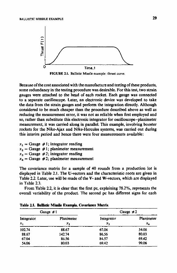
FIGURE 2.1. Ballistic Missile example: thrust curve.

Because ofthe cost associated with the manufacture and testing of these products, some redundancy in the testing procedure was desirable. For this test, two strain gauges were attached to the head of each rocket. Each gauge was connected to a separate oscilloscope. Later, an electronic device was developed to take the data from the strain gauges and perform the integration directly. Although considered to be much cheaper than the procedure described above as well as reducing the measurement error, it was not as reliable when first employed and so, rather than substitute this electronic integrator for oscilloscope-planimeter measurement, it was carried along in parallel. This example, involving booster rockets for the Nike-Ajax and Nike-Hercules systems, was carried out during this interim period and hence there were four measurements available:

xI = Gauge # 1; integrator reading x2 = Gauge # 1; planimeter measurement x3 = Gauge #2; integrator reading x4 = Gauge # 2; planimeter measurement

The covariance matrix for a sample of 40 rounds from a production lot is displayed in Table 2.1. The U-vectors and the characteristic roots are given in Table 2.2. Later, use will be made of the V- and W-vectors, which are displayed in Table 2.3.

From Table 2.2, it is clear that the first pc, explaining 78.2%, represents the overall variability of the product. The second pc has different signs for each

Table 2.1. Ballistic Missile Example. Covariance Matrix ~~ ~~ ~~

Gauge # l Gauge #2

Integrator Planimeter Integrator Planimeter X1 x2 x3 x4

102.74 88.67 67.04 54.06 88.67 142.74 86.56 80.03 67.04 86.56 84.57 69.42 54.06 80.03 69.42 99.06

30 PCA WITH MORE THAN TWO VARIABLES

Table 2.2. Ballistic Missile Example. Characteristic Roots and U-Vectors

U1 "2 u3 u4

XI .468 - .622 .572 - .261 Xl .608 -.179 - .760 -.147 x3 .459 .139 .168 .861

Characteristic root 335.34 48.03 29.33 16.4 1 % Explained 78.1 11.2 6.8 3.8

x4 .448 .750 .262 -.410

Table 2.3. Ballistic Missile Example. V- and W-vectors

V 1 v2 v3 v4 Wl w2 w3 w4

X1 8.57 -4.31 3.10 -1.06 .0256 -.0897 .lo55 -.0643 ~2 11.13 -1.24 -4.11 -.60 .0332 -.0258 -.1402 -.0364 ~3 8.41 .96 -91 3.49 .0251 .0200 .0310 .2126 ~4 8.20 5.20 1.42 -1.66 .0245 ,1082 ,0483 -.lo13

gauge and hence represents gauge differences. The other two pc's are less clear. A case might be made for integrator-planimeter differences related to Gauge # 1 for y, and for Gauge #2 for y4 but the results may not prove overly convincing and more will be said about this in Section 2.6. If one is willing to accept, for the moment, that these last two pc's represent some sort of testing and measurement variability, then one can conclude that, on the basis of this sample, roughly 78% of the total variability is product and 22% is testing and measurement. The Army had required, with each released production lot, an estimate of the proportion of the total reported variability that could be attributed to testing and measurement and PCA was one of the methods proposed to produce this estimate (Jackson, 1960).

2.4 COVARIANCE MATRICES OF LESS THAN FULL RANK

Before going on to some new procedures required when one has more than two variables, it may be advisable to digress, briefly, to consider a special case of covariance matrix that is not of full rank. This situation will occur when one or more linear relationships exist among the original variables so that the knowledge of a subset of these variables would allow one to determine the remainder of the variables without error.

As an example, let us return to our chemical example and add a third variable, which will be the sum of the first two, that is, x, = x1 + x2. This is a case of a linear relationship because the sum of the first two variables uniquely determines the third. x, adds no information whatsoever. The covariance matrix

COVARIANCE MATRICES OF LESS THAN FULL RANK 31

now becomes

1 ,7986 A793 1.4779

.6793 .7343 1.4136 1.4779 1.4136 2.8915

The third row and column are the result of the new variable, x3. The other four quantities are the same as for the two-dimensional case. The characteristic roots of this matrix are 4.3880, .0864, and 0. These roots are directly related to the roots for the two-dimensional case. The first root, 4.3880, is equal to the first root for p = 2, 1.4465, plus the variance of x3, 2.8915. The second root is the same as it was for p = 2. The third root is zero, indicating that the covariance matrix is not of full rank and there exists one linear relationship among the variables. In general the rank of a matrix will be reduced by 1 for each of these relationships.

The U-vectors corresponding to these roots are

.4174 -.7017 -.5774

.3990 .7124 -.5774 3164 .0107 S774

The coefficients in the first vector, not surprisingly, show that, ~ 3 1 = ul l + uzl. All of the coefficients are still positive because all three values, generally, rise and fall together. The second vector is essentially xz - x1 as it was before, but in this case, as with ul, the third coefficient equals the sum of the first two. Since the third vector is associated with a zero root, do we need to bother with it? The answer is “yes” because u3 explains a linear relationship. The coefficients are all equal except for sign and tell us that

-x1 - xz + xs = 0

or

x1 + xp = x3

The existence of a zero root, li = 0 implies that zi = u;[x - Z] = 0 for any x and hence, u’[x - fi]’Cx - %]u/(n - 1) = It = 0.

The V-vectors are:

.8695 -.2063 0 [ 3309 .2094 03

1.7004 .0031 0


The third vector is zero because it is normalized to its root, zero, and hence has no length. This means that the covariance matrix can be reconstructed from vi and v2 alone. Another simple demonstration example may be found in Ramsey (1986). For the W-matrix, the corresponding third vector is undefined.

The practical implication of this is that an unsuspecting analyst may, from time to time, receive some multivariate data with one or more linear relationships (sums and differences being the most common) placed there by a well-intentioned client who did not realize that multivariate analysis abhors singular matrices. Many computer packages have, as an option, the ability to obtain all of the characteristic roots. Whenever the data are suspect, this should be done. The existence of one or more zero roots is prima facie evidence that trouble exists. An investigation of the vectors associated with them may give a clue as to what this trouble is. Even if one is not interested in performing a PCA on these data, in the first place, this technique can still be useful in such occurrences as singular X’X matrices in multiple regression or its counterpart in MANOVA or discriminant analysis.

Examples of such constraints in a chemical problem along with the interpretation of the vectors associated with the zero roots may be found in Box et al. (1973). They pointed out that because of rounding, these roots may be positive rather than zero but would be so much smaller than the others that they should be detected anyhow. (See Section 2.8.5 on SCREE plots.)

Another cause of singular covariance matrices is the result of having more variables than observations. If n < p, then the maximum number of nonzero roots will be n - 1.

2.5 CHARACTERISTIC ROOTS ARE EQUAL OR NEARLY SO

Another anomaly of characteristic roots is the case where two or more of the roots are equal to each other. The simplest case of this would be for the case p = 2 where the two variances are equal and the variables are uncorrelated. The characteristic roots will be equal (and equal to the variances) and the ellipse defined by this will, in fact, be a circle. The major and minor axes will be of equal length and can be anywhere as long as they are orthogonal. This means that the vector orientation is undefined. In the more general case, any time there are two or more equal roots, that part of the orientation will be undefined even though there are distinct roots that are both larger and smaller.

Unless one is working with patterned matrices, the probability of the occurrence of identically equal roots in a real data set is remote, but what can occur is the existence of two or more roots that are nearly equal. As will be seen in Chapter 4, the standard errors of the coefficients of characteristic vectors are a function of the separation of these roots; these standard errors can become inflated by the occurrence of two or more roots close to each other. This means that even though the orientation of the axes is defined, it is not defined with very much precision and hence attempts to interpret these pc’s might be unwise.

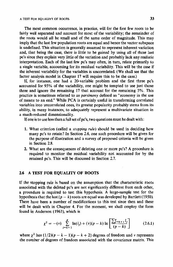
A TEST FOR EQUALITY OF ROOTS 33

The most common occurrence, in practice, will for the first few roots to be fairly well separated and account for most of the variability; the remainder of the roots would all be small and of the same order of magnitude. This may imply that the last few population roots are equal and hence the vector subspace is undefined. This situation is generally assumed to represent inherent variation and, that being the case, there is little to be gained by using all of these last pc’s since they explain very little of the variation and probably lack any realistic interpretation. Each of the last few pc’s may often, in turn, relate primarily to a single variable, accounting for its residual variability. This will be the case if the inherent variability for the variables is uncorrelated. (We shall see that the factor analysis model in Chapter 17 will require this to be the case.)

If, for instance, one had a 20-variable probiem and the first three pc’s accounted for 95% of the variability, one might be tempted to use just those three and ignore the remaining 17 that account for the remaining 5%. This practice is sometimes referred to as parsimony defined as “economy in the use of means to an end.” While PCA is certainly useful in transforming correlated variables into uncorrelated ones, its greater popularity probably stems from its ability, in many instances, to adequately represent a multivariate situation in a much-reduced dimensionality.

If one is to use less than a full set of pc’s, two questions must be dealt with:

What criterion (called a stopping rule) should be used in deciding how many pc’s to retain? In Section 2.6, one such procedure will be given for the purpose of illustration and a survey of proposed criteria will be given in Section 2.8. What are the consequences of deleting one or more pc’s? A procedure is required to monitor the residual variability not accounted for by the retained pc’s. This will be discussed in Section 2.7.

2.6 A TEST FOR EQUALITY OF ROOTS

If the stopping rule is based on the assumption that the characteristic roots associated with the deleted pc’s are not significantly different from each other, a procedure is required to test this hypothesis. A large-sample test for the hypothesis that the last (p - k) roots are equal was developed by Bartlett (1950). There have been a number of modifications to this test since then and these will be dealt with in Chapter 4. For the moment, we shall employ the form found in Anderson (1963), which is

(2.6.1 ) P

j = k + 1 x2 = -(v) ln(lj) + (v)(p - k) In

where x2 has (1/2)(p - k - l)(p - k + 2) degrees of freedom and v represents the number of degrees of freedom associated with the covariance matrix. This


test can be performed after each stage, keeping in mind the effect on the Type I error by making successive tests. If the remaining roots are not significantly different from each other, the procedure is terminated at that point. (Some computer programs obtain all of the roots at once so this test could be incorporated to produce a series of tests before any of the vectors are obtained.) If the final number of pc’s retained is k, formula (1.7.5) for T: must be modified by replacing p with k.

Turning to the Ballistics Missile example in Section 2.3, the first test that could be applied is for the hypothesis

H,: A, = A, = A, = 1,

against the alternative that at least one root was different. For this hypothesis,

x 2 = -(39)[ln (335.34) + + In (16.41)]

= 110.67

with 9 degrees of freedom, which is highly significant. A test of the next hypothesis,

H,: 1, = A3 = A,

which says, “Given that A, is different from the others, are the others equal?”, produces a value of x2 = 10.85 which, with 5 degrees of freedom, is not quite significant at the 5 % level. A test of H,: A3 = 2, yields a value of x 2 = 3.23 which, with 2 degrees of freedom, is not even close. If the sample size were 100 instead of 40, for the same covariance matrix, all four roots would have tested out to be significantly different.

If the percentage of the trace unexplained by the significant pc’s is appreciable, this is an indication that these pc’s are not doing an acceptable job of spanning the space generated by the data. This is not necessarily a disaster. It may be that most of the variability is random variability associated with the original variables, and if this is large relative to the total trace it simply means that the original variables do not have that much in common. Parsimony is desirable but not always obtainable.

2.7 RESIDUAL ANALYSIS

2.7.1 Introduction

In Section 1.5.5, it was shown that if one used a full set of pc’s, it was possible to invert the equation that produced the pc’s from the data and, instead,

RESIDUAL ANALYSIS 35

determine the original data from the pc’s. Since most of the applications in this book scale the pc’s to have unit variances, we can rewrite equation (1.5.5)

x = % + U z

as

x = % + V y (2.7.1)

However, x will be determined exactly only if all the pc’s are used. If k < p pc’s are used, only an estimate Q of x will be produced, viz.,

*=%+Vy (2.7.2)

where V is now p x k and y is k x 1. Equation (2.7.2) can be rewritten as

x = % + vy + (x - 2) (2.7.3)

a type of expression similar to those often found in other linear models. In this case, the first term on the right-hand side of the equation represents the contribution of the multivariate mean, the second term represents the contribution due to the pc’s, and the final term represents the amount that is unexplained by the pc model-the residual. Wherever any pc’s are deleted, some provision should be made to check the residual.

Gnanadesikan and Kettenring ( 1972) divided multivariate analysis into

1. The analysis of internal structure. 2. The analysis of superimposed or extraneous structure.

There are outliers associated with each of these and it is important to keep their identities distinct. (Hawkins refers to these as Type A and Type B outliers.)

The “Type A” outlier refers to a general outlier from the distribution form one wishes to assume. Usually this assumption will be multivariate normal and these outliers will be detected by large values of T2 and/or large absolute values of the y- or z-scores such as the example in Section 1.7. The important thing about this type of outlier is that it would be an outlier whether or not PCA has been employed and hence could be picked up by conventional multivariate techniques without using PCA. However, the use of PCA might well enhance the chance of detecting it as well as diagnosing what the problem might be.

In this section, we will be concerned with the “Type B” outlier, the third term in (2.7.3)’ which is an indication that a particular observation vector cannot be adequately characterized by the subset of pc’s one chose to use. This result can occur either because too few pc’s were retained to produce a good model or because the observation is, truly, an outlier from the model. It is also possible in repetitive operations, such as quality control, that the underlying covariance


structure and its associated vector space may change with time. This would lead to a general lack-of-fit by the originally defined pc’s.

2.7.2 The @Statistic

The residual term of (2.7.3) can be tested by means of the sum of squares of the residuals:

Q = (X - n)’(x - 2) (2.7.4)

This represents the sum of squares of the distance of x - S from the k- dimensional space that the PCA model defines. [A form of this statistic was first proposed by Jackson and Morris, (1957), but the X*-approximation that they used for that statistic is incorrect and should not be used.]

To obtain an upper limit for Q, let:

P

el = c ii i = k + l

i = k + l

P 03 = 1 1:

i = k + l

and

Then the quantity

(2.7.5)

is approximately normally distributed with zero mean and unit variance (Jackson and Mudholkar, 1979). Conversely, the critical value for Q is

(2.7.6)

where c, is the normal deviate cutting off an area of a under the upper tail of the distribution if h, is positive and under the lower tail if ho is negative. This

RESIDUAL ANALYSIS 37

distribution holds whether or not all of the significant components are used or even if some nonsignificant ones are employed.

It should be noted that Q can also be written as

P P

Q = C I& = C ~f i = k + l i = k + l

(2.7.7)

so that Q is a weighted sum of squares of the last p - k components. Although this may be thought of as an alternative method of computing Q, it does not require the calculation of all the pc’s and does not produce [x - n] directly. [In the form of equation (2.7.7), Q is sometimes referred to as the Rao-statistic. A number of texts state that it has an asymptotic X’-distribution but this, like the Jackson-Morris conjecture mentioned earlier, is incorrect.]

In Section 2.6, it was suggested that the last two characteristic roots in the Ballistic Missile example were not significantly different from each other and hence the last two pc’s should be deleted. If only the first two pc’s were retained, what would be the limit for Q? The last two roots were 29.33 and 16.41. From these, O1 = 45.74,O’ = 1129.54, O3 = 29 650.12, and from these ho = .291. Letting a = .05, the limit for Q, using (2.7.6) is

(1.645)J(2)(1129.54)(.291)’ (1129.54)(.291)( -.709) 11*z91

+ l l +

45.74 (45.74)’ Q.05 = 45.74

= 140.45

Values of Q higher than this are an indication that a data vector cannot be adequately represented by a two-component model.

Now let us assume that a new round is tested with the results

X = [ ”1 - 5

and assume that the mean is zero. Using the first two columns of W in Table 2.3, the y-scores are

The a = .05 limits for the pc’s for n = 40 are k2.20 so neither of these are significant. TZ = 4.2383, which is also not significant when compared with its


limit of 6.67. The predicted test values, given these pc’s, are

again, using the first two columns of V in Table 2.3. The residuals are

and their sum of squares is Q = (x - S)’(x - 2) = 202.2, which is significant. The conclusion is that the two-component model does not fit the data and the culprit appears to be a mismatch between the results on the second gauge. Note that if the other pc’s had been computed, y, = 3 9 and y4 = 3.430. Then, verifying (2.7.7),

(29.33)(.559)’ + (16.41)(3.430)’ = 202.2

It has been the experience of many practitioners, particularly but not restricted to the engineering and physical sciences, that the greatest utility of the Q-statistic (or the alternatives discussed below) is its ability to detect bad data, measurement errors, and the like. Every set of multivariate data that is to be subjected to PCA should be screened using one of these statistics. Some people use PCA, including the residual test, for screening multivariate data even though they have no intention of using the pc’s afterward. We shall find a number of instances in this book where Q has also been used as an intermediate step in a particular procedure.

In obtaining the Bi’s, if one has a large number of deleted pc’s, one is faced with having to obtain not only all of the characteristic roots associated with them but with their squares and cubes as well. There is a short cut for this because we are not interested in the individual roots but only their sums. Let E be the residual covariance matrix after k characteristic vectors have been extracted. Then

B1 = Tr(E)

6’ = Tr(E2)

O3 = Tr(E3)

(2.7.8)

(2.7.9)

(2.7.10)

a user’s guide to principal components - semantic scholar · a user's guide to principal...

Documents