lable at ScienceDirect

Environmental Modelling & Software 82 (2016) 308e320

Contents lists avai

Environmental Modelling & Software

journal homepage: www.elsevier .com/locate/envsoft

A user-driven case-based reasoning tool for infilling missing values indaily mean river flow records

Laura Giustarini*, Olivier Parisot, Mohammad Ghoniem, Renaud Hostache, Ivonne Trebs,Benoît OtjacquesLuxembourg Institute of Science and Technology (LIST), Environmental Research & Innovation Department (ERIN), 5, avenue des Hauts-Fourneaux, L-4362Esch/Alzette, Luxembourg

a r t i c l e i n f o

Article history:Received 19 November 2015Received in revised form23 March 2016Accepted 12 April 2016

Keywords:Gap fillingHydrological time seriesCase-based reasoningKnowledge databaseHuman in the loop

* Corresponding author.E-mail address: laura.giustarini@gmail.com (L. Giu

http://dx.doi.org/10.1016/j.envsoft.2016.04.0131364-8152/© 2016 Elsevier Ltd. All rights reserved.

a b s t r a c t

Missing data in river flow records represent a loss of information and a serious drawback in watermanagement. In this work, we introduce gapIt, a user-driven case-based reasoning tool for infilling gapsin daily mean river flow records. Given a set of flow time series, gapIt builds a database of artificial gapsfor which it computes several flow estimates, to find the best combinations of infilling algorithm andautomatically selected donor station(s), according to state-of-the-art performance indicators. We ob-tained satisfactory results with Nash-Sutcliffe >0.7 for more than half of the ~5000 synthetic gaps ofvarious lengths and positions, randomly created along the available records. gapIt was evaluated on 24daily river discharge time series recorded in Luxembourg over seven years from 01/01/2007 to 31/12/2013. We also discuss the benefits of coupling this approach with user-expertise for an improved infillingof real data gaps.

© 2016 Elsevier Ltd. All rights reserved.

Software availability

Name of software: gapItDeveloper: Olivier Parisot (olivier.parisot@list.lu)Programming language: JavaRequired hardware: 4 GB RAM minimumSupported systems: Windows, Unix, Linux, MacRequired softwares: Maven (�3.0.2), JDK (�1.7)Availability: https://github.com/ERIN-LIST/gapItLicense: GNU General Public License version 3

1. Introduction

Long uninterrupted hydrological time series are often notavailable for many of the stream gauges in the world. Rather, timeseries of hydrological data are often affected by data gaps, whichare discontinuities in the record of data. They are an inevitableconsequence of factors such as station maintenance, equipmentmalfunctioning, human errors, changes in instrumentation anddata processing issues (Harvey et al., 2010). Missing data in river

starini).

flow records represent a loss of information and a serious drawbackinwater management. The existence of gaps results in difficulties indata interpretation and is a large source of uncertainty in dataanalysis. Specifically, the presence of discontinuities precludes thecomputation of hydrological statistics and physiographic indices. Italso limits the use of such data for hydrological or hydrodynamicmodel calibration/validation purposes. A consequence of these is-sues is the need of data infilling methods to reconstruct missingdata, when appropriate and before hydrological time series can beused in a number of applications.

From a technical point of view, a wide choice of data analysistools is nowadays offered to hydrologists. For instance, specific userfriendly software tools are already available or can be developed inplatforms like R1 or Matlab2 to interpolate missing data and/oraddress hydrological problems. But most of these tools requiresome data mining and machine learning expertise, as well as fine-tuning in order to meet user needs and be properly exploitable byend-users (Serban et al., 2013). As a result, hydrologists have accessto a collection of usable tools, but they still need to deal with severaltechnical issues (like data wrangling, tuning predictive algorithms)

1 http://www.r-project.org/.2 http://www.mathworks.com/products/matlab/.

3 http://www.hydroclimato.lu.

L. Giustarini et al. / Environmental Modelling & Software 82 (2016) 308e320 309

before solving their initial problem, i.e. infilling missing values.Data infilling is a challenging task that has been addressed by

previous research work.

2. Related work

For infilling gaps in hydrological time series, classical methodsof data analysis have long been applied (Salas, 1980) and recentstudies have proposed more efficient techniques (Harvey et al.,2010; Mwale et al., 2012). Most of the methods proposed in theliterature are based on data transfer from one or more donor sta-tions (gauges) to a target station. Among all possible infillingmethods, the choice of themost appropriate one is not a trivial task.The same holds true for the selection of a set of donor stations.Moreover, results greatly depend on the context and, in non auto-mated techniques, also on the user expertise.

Recently, Harvey et al. (2010) tested different infilling tech-niques, simulating an entire target flow record, for several stationsin the UK. For each target station, two donor stations were selecteda priori, based on the hydrological knowledge of the region andcatchment metadata. Their work focused on the performanceanalysis of gap infilling techniques. In a follow-up study, Harveyet al. (2012) assessed a wide range of target-donor combinations,trying at the same time to improve data infilling performance byeither seasonally grouping flows or excluding knowninhomogeneity.

Gyau-Boakye and Schultz (1994) presented a Decision SupportSystem (DSS) for selecting themost appropriate infillingmodel, as afunction of gap length, season, climatic region and data character-istics of the records. The main disadvantage of their approach isthat all rules are hard-coded and specific to a given region, namelyWest Africa. The same idea was applied by Johnston (1999) to builda DSS that helps experts select an estimation method for missingrainfall data in the United States. More recently, Griffioen et al.(2006) proposed a Case-Based Reasoning system (CBR) to inter-compare water stress among different catchments in Europe. Intheir work, CBR was presented as a retrieval method to offer largeamounts of filtered information to the end-user. In a broadercontext, Matthies et al. (2007) provided a review on environmentalDSS, showing a general tendency towards integration and visuali-zation of temporal and spatial results.

Despite the numerous studies available in the literature, astandardized procedure for gap filling in hydrological time series isstill missing. One of the main limitations of many of the currentlyavailable approaches is their incomplete level of automation.Generally, donor stations are often determined a priori and tend tobe specific to only a given region of interest. The user expertise isfundamental for this type of settings but it also limits the level ofautomation and the transferability of the approach to differentareas.

In this work, we present a first attempt towards standardization,providing an interactive tool that allows performing gap filling in aconsistent and traceable manner, bridging the gap between data-driven and user-expertise approaches.

gapIt is an interactive and visual data-driven tool that offersseveral infilling techniques, coupled with different sets of donorstations. It assesses the performance of all possible configurations,i.e. combinations of infilling method and set of donor station(s), tofill a given gap in a consistent way, eventually providing the bestdata-driven solution according to performance indicators. The vi-sual interface allows users to select different infilling methods and/or donor station(s) than those automatically proposed by the tool,according to their expertise and specific knowledge of the region ofinterest. The fact that users can interactively inject their knowledgeallows an iterative refinement of the results, while keeping track of

all modifications.In the general practice, infilling techniques require both a strong

methodological background and a significant knowledge of theapplication domain (Maimon and Rokach, 2005; Domingos, 2012).In this paper, we show how gapIt can provide a bridge between apurely data-driven approach and an infilling method based on userexpertise only. The automated approach, coupled with a visual in-spection system for user-defined refinement, allows for standard-ized infilling, where subjective expert decisions can easily beincorporated in a traceable manner.

In the remainder of this paper, we will present a case study andthe related data sources (section 3). Then we describe the pro-posed gapIt algorithm in section 4, which is followed by ananalysis of the results obtained for both synthetic and real gaps insection 5. Advantages and limitations of the method are summa-rized at the end.

3. Case study

The dense river network of hydrometric stations in Luxembourgoffers an excellent opportunity to test the proposed tool. The gaugenetwork considered here is composed of 24 stations, displayed inFig. 1, including both very responsive and groundwater-fed rivers.The region has a temperate, semi-oceanic climate. Precipitation isrelatively uniform throughout the year, although strong seasonalityin low flow exists due to higher evapotranspiration from July toSeptember. High discharge values are recorded in winter(maximum JanuaryeFebruary), sometimes leading to inundations,while low flows are observed particularly in September. The in-fluence of snow can be considered negligible.3

We use discharge data, originally available as 15-min time seriesand subsequently aggregated using gapIt itself to daily values,covering the period from 01/01/2007 to 31/12/2013. A total numberof 28 gaps are present in the dataset; most of them have beenobserved in winter.

4. Methods and tools

In this section, algorithm implementation and input data re-quirements for gapIt will be described. It has to be noted that thisapproach is based on a single variable, discharge, provided as inputto the software. This loosens dependency on other types of vari-ables, for instance catchment rainfall, which may not always beavailable (Harvey et al., 2010). In the following, we designate astarget station (respectively, donor station(s)) the station charac-terized by a gap to be infilled (respectively, the station(s) whosedata is used to derive infilled data for the target). The underlyinghypothesis of the presented tool is the availability of a sufficientlydense river network that provides continuous measurements. gapItinfills gaps in discharge time series, providing the final user withthe best solution that is possible to obtain, given the available donorstations. The best solution is individuated based on performancemeasures. As we are dealing with both synthetic and real gaps, twodifferent strategies will be proposed to compute performancemeasures, depending on the type of gap. The insertion of estimatedvalues in the database in lieu of gaps is subject to the acceptance bythe end-user.

All infilled data are consistently flagged, for the sake of trace-ability of the reconstructed values. Moreover, the configurationused for infilling each gap is stored in the database, for the sake ofreproducibility.

Fig. 1. Gauging stations in the river network of Luxembourg. The upper right panel shows the location of Luxembourg in North West Europe.

L. Giustarini et al. / Environmental Modelling & Software 82 (2016) 308e320310

4.1. Software architecture and third-party libraries

gapIt is a multiplatform standalone tool developed in Java. It ismainly based on Cadral, a data analysis platform (Didry et al., 2015)developed in-house and leveraging WEKA (Witten et al., 2011) fordata mining purposes, and JFreeChart (Gilbert, 2002) for graphicaldata representation.

4.2. Input data

gapIt is capable of importing/exporting data in CSV format or inWEKA's ARFF format. The data infilling process uses the followinginput data:

� Time series of hydrological data (discharge), recorded at severalgauging stations within the river network described earlier. Foreach station, the data consists of a sequence of numerical valueswith timestamps.

� Geographic coordinates of gauging stations (longitudes andlatitudes).

� Upstream/downstream relationships (if applicable, dependingon the stations); this information is stored in the form of a de-pendency graph, a simple scheme displaying the different re-lationships among stations.

In case an upstream/downstream station is not present oravailable in the same river as the target station, we use the closeststation in a tributary as a proxy upstream gauge and, as a proxydownstream gauge, the closest station in the river where thestream with the target station flows.

4.3. Visualization and data preprocessing

A graphical user interface (GUI) allows the visual inspection ofdata, in terms of time series, maps and relationships. The user cantypically visualize the different gaps (Fig. 2) in their spatio-temporal context. The GUI consists of three panels showing:

� The list of gaps present in all time series (Fig. 2, panel 1).� A map (Fig. 2, panel 2) showing the locations of the gaugingstations. Based on the user selection, the gauge of interest isinteractively highlighted, to easily put it in its geographiccontext.

� A line chart (Fig. 2, panel 3) to let end-users inspect temporaltrends of the selected time series and put gaps in their temporalcontext.

Moreover, the tool offers several data preprocessing features. Inparticular, the user can set the desired temporal resolution of the

Fig. 2. Graphical user interface of gapIt: (1) gap list, (2) map showing the locations of the available stations, (3) time series visualization.

L. Giustarini et al. / Environmental Modelling & Software 82 (2016) 308e320 311

time series, i.e. creating hourly, daily andmonthly aggregate values.In the present study, it was deemed more appropriate to performgap infilling on daily values, rather than on the noisier original 15-min observations (Harvey et al., 2010, 2012).

4.4. Gap characterization and inspection

The choice of any particular gap-filling technique depends onseveral factors: gap length, season, high/low flow conditions, etc.(Gyau-Boakye and Schultz, 1994). As a consequence, these charac-teristics are determined in gapIt and are accessible by the userthrough the GUI (Fig. 2).

� Flow (low/medium/high): given the minimum and maximumvalue of a certain time series (i.e. station), three equispacedranges are defined in order to characterize the type of flowbefore and after a gap.

� Rising limb: an outlier detection method is used to detect thepresence of a rising limb, which may indicate the probablepresence of a flood event for the considered gap. More precisely,the method is based on the local outlier factorwhich computes ascore for each value of the time series by taking into accountvalues before and after it (Breunig et al., 2000).

� Geographical proximity: the closest station is computed byapplying a simple Euclidean distance on station coordinates.

� Upstream/downstream relationships: the identification of up-stream and downstream station(s), if present, is carried out onthe basis of the input dependency graph, using a simple nearest-neighbor search.

� Similarity between time series: this is computed using DynamicTimeWarping (DTW) (Berndt and Clifford,1994). This method israther popular in time series analysis as it takes into accounttime shift and distortion and was already used in hydrology tofind patterns in discharge data (Ouyang et al., 2010). In practice,due to the high time complexity of DTW, we use an empiricallydefined timewindow of size N*gapsize (with N fixed by the end-user e a reasonable value for N between 3 and 10 helps defininga compact and sufficient time window).

These properties are computed and displayed in the GUI (Fig. 2).

4.5. Gap infilling

To fill a given gap, we propose a two-phase approach describedin Algorithm 1: the tool starts by computing the best solutionautomatically. Then, the end-user can either accept or refine it.

L. Giustarini et al. / Environmental Modelling & Software 82 (2016) 308e320312

More precisely, different configurations are considered to infill agap. By configuration we mean a combination of donor station(s)and gap infilling method. For a given gap, gapIt computes allpossible configurations and ranks them according to errors andperformance measures (Section 4.6). The best configuration isautomatically selected by the tool as the one yielding the smallestroot mean squared error (RMSE) (Please see Section 4.6 for moredetails). Subsequently, the user/expert can refine it by adjusting anyof its constituents.

Eventually, the configuration approved by the user is applied toreconstruct the missing data which gapIt stores and flags as infilleddata.

4.5.1. Selection of the donor stationsSelecting donor stations represents the most critical step of the

infilling procedure, as their data is going to be used to estimate themissing values. Based on the gap characterization data (Section4.4), the software offers several options to automatically selectdonor station(s) among:

� the geographically closest station;� the station having the most similar time series (based on DTWas explained in Section 4.4);

� the upstream and/or downstream station.

It is important to highlight that both the geographically closeststation and the onewith themost similar time seriesmay not belongto the same catchment as the target station. In addition, all differentcombinations of donor stations are potentially applicable dependingon the case at hand. For example, the algorithm and/or the user mayuse the downstream station and ignore the geographically closestone. The final set of donor stations depends on several factors, suchas the context, and user expertise, among others.

4 http://commons.apache.org/proper/commons-math/index.html.

4.5.2. Selection of an infilling methodObservations with missing data can of course simply be

omitted in the user application: this trivial approach can be suf-ficient in several cases (Enders, 2010) or when infilling may risk

being detrimental (Beven and Westerberg, 2011; Beven and Smith,2014) leading to periods of disinformative hydrological data.However, it goes without saying that data infilling is an extremelyhelpful approach to make the best possible use of time series, forexample to derive accurate long-term statistics. Dealing withmissing values is a well-known topic in data mining and ap-proaches generally used in this field can be easily transferred tohydrology.

Among the various infilling methods proposed in the literature(Pigott, 2001; Marwala and Global, 2009; Van Buuren, 2012), acomprehensive, though not exhaustive, range of available methodswas selected and integrated into gapIt:

� Interpolation (INTERP) is an easy and efficient solution if timeseries do not present steep increases or decreases of measuredvalues (jumps) in data and when the gap length is rather small.

� Mean value (ZeroR) is a simple solution that consists inreplacing missing numerical values by the mean value: thisapproach is still used in many statistical software packages.However, it can highly disrupt the data structure, thus degrad-ing the performance of statistical modelling (Junninen et al.,2004). In this paper, we use Weka's ZeroR classifier.

� The Nearest-neighbors (NN) technique as implemented inWekawas applied as follows: for each incomplete record, similar re-cords are identified (by using the Euclidean distance as a bruteforce search) among the already selected donor stations, andthen used to estimate missing values.

� Multiple linear regressions (REG) are rather frequently used,particularly when links are evident among sensors of thenetwork: they can capture relationships between downstreamand upstream gauges (Bennis et al., 1997). In gapIt, we inte-grated the Ordinary Least Square method, provided by theApache Commons Mathematics Library.4

� Regression Trees (RT) are suitable too as they are efficient andeasy to visualize/interpret (Kotsiantis, 2013): rules are explicitly

L. Giustarini et al. / Environmental Modelling & Software 82 (2016) 308e320 313

described by the tree and are more expressive than the classicallinear regression formula (Witten et al., 2011, section 3.3). gapItuses Weka's REPTree implementation.

� Model trees (MT) are included by applying the M5 method(Quinlan, 1992); this technique was recently used to forecastflows in Turkey (Sattari et al., 2013). gapIt uses Weka's M5Pimplementation (Witten et al., 2011, section 6.6).

� Artificial Neural Networks (ANN) have been recently used topreprocess missing hydrological data (Mwale et al., 2012; Tfwalaet al., 2013). Although some work has been done to ease theinterpretation of ANN (F�eraud and Cl�erot, 2002), they are stilldiscounted as black box models. Yet, they represent anextremely helpful approach to build powerful predictivemodels, capable of providing satisfactory results. gapIt uses theimplementation of the multilayer perceptron with back propa-gation (Witten et al., 2011, section 6.4).

� Expectation-Maximization (EM) method (Van Hulse andKhoshgoftaar, 2008) was also included in gapIt, through aWeka plugin which uses EM to replace missing values with amultivariate normal model.5

The above listed techniques are implemented and available ingapIt. As a complement to all of them, temporal discretization isincluded as an additional option. In other words, for all the eightmethods implemented in gapIt, when applicable, one test is madeconsidering the discretization in time of the governing equations,while the second computation is performed excluding this addi-tional step. The idea behind this is to take the best advantage oftime discretization in all cases where it helps the algorithm incapturing temporal patterns (i.e. adding date-derived periodic at-tributes like month of the year or quarter).6

While the application of ANN is accepted as a form of rainfall-runoff modelling (Gao et al., 2015), it has to be noted that con-ventional hydrological modelling was not included in this work.According to Harvey et al. (2010), current rainfall-runoff models arestill too demanding in terms of computation time, resources andinput data, with the need of calibration limiting transferabilityamong catchments.

More sophisticated techniques, like flow-flow models for donorstations, as well as forms of inverse hydrology (Croke, 2006;Kirchner, 2009; Kretzschmar et al., 2014) could be implementedin gapIt. However, for themomentwe deliberately intended to limitthe involved inputs and the required knowledge and systemic un-derstanding of hydrological processes.

4.6. Evaluation of the infilling accuracy

Eventually, the user can inspect the results in the GUI, togetherwith an evaluation of the infilling performance (Fig. 3). The accu-racy of the gap-filling procedure can be assessed using several er-rors and performance measures: RMSE, mean absolute error (MAE)and Nash-Sutcliffe coefficient (NS) (Nash and Sutcliffe, 1970). Inpractice, a perfect gap infilling will lead to MAE and RMSE valuesequal to 0 and an NS value of 1. In the literature, ranges of satis-factory fits are provided for various performance indicators(Moriasi et al., 2007a; Harmal et al., 2014). The NS coefficient isfrequently used in hydrology and has the interesting characteristicof being dimensionless, which allows the comparison betweendifferent catchments and periods. Its main limitation lies in the factthat the differences between observed and predicted values aresquared. Thus, larger values in a time series are overestimated

5 http://weka.sourceforge.net/packageMetaData/EMImputation/index.html.6 http://tinyurl.com/padzrt4.

while lower values are neglected (Krause et al., 2005; Legates andMcCabe, 1999). This leads to an overestimation of the model per-formance during peak flows and an underestimation during lowflow conditions. One should also note that all performance in-dicators have their shortcomings. For example, the index ofagreement leads to relatively high values even for poor model fitsand, like the NS, is not sensitive to systematic model over- orunderprediction. Other additional measures are implemented inthe tool, like the index of agreement and the percent bias (PBIAS)(Moriasi et al., 2007b), but they are not included in this study forthe sake of brevity.

As anticipated we deal with both synthetic and real gaps and,correspondingly, the strategy to compute the evaluation measuresslightly differs for the two situations.

4.6.1. Infilling accuracy for synthetic gapsIn the case of a synthetic gap, the estimated series for gap

infilling is compared to the actual observations, only in the timewindow of the gap itself (Evaluation strategy A). Visually, the toolsimply presents the result by indicating the errors and by plottingthe observed and estimated time series on the same plot (Fig. 4).

4.6.2. Infilling accuracy for real gapsIn contrast, when dealing with a real gap, the software will first

individuate a time window that is centered on the gap itself butlarger than it. The enlargement is set as a percentage of the gap sizeitself. The infilling performance (Evaluation strategy B) is computedon values before and after a given real gap, where observed valuesare available.

Obviously in case of a real gap, the performance measures canonly hint to the algorithm performance, as they are computed overa period that does not exactly match the time span of the gap.

4.7. Selection of the best solution

In conclusion, after computing all possible configurations, i.e.donor station(s) and infilling methods, the software will automat-ically provide the best solution, characterized by an optimalconfiguration, i.e. the one yielding the smallest RMSE (Evaluationstrategy A for synthetic gaps, Evaluation strategy B for real gaps). Allother indicators, e.g. NS, index of agreement, are provided to theuser to better contextualize the infilling performance and accuracy.The user can always adjust the configuration, to identify the solu-tion that is deemed the most appropriate. The user expertise rep-resents an invaluable resource to interpret the results and improveand/or reject model outputs.

The best solution retained in the end can be different from theone initially found by the algorithm in a purely data-drivenapproach. Users may simply accept the solution with the bestperformance measures or use it as a starting point, to be refinedbased on their expertise, by adjusting the configuration. They canalso completely discard the proposed solution, leaving the gapunfilled if none of the configurations is deemed appropriate. Thiskind of post-processing combines the best of a data-drivenapproach and a manual infilling based on the human knowledgeof the problem/context.

4.8. A case-based reasoning module for traceability and decisionsupport

For a given gap (synthetic/real), gapIt determines the best so-lution as the one with the best performance (Evaluation strategyA/B), given the available inputs. However, to take the bestadvantage of the tool, a knowledge database can be built withsynthetic gaps appropriately created and infilled. In this case, to

Fig. 3. User interface to visualize and infill a true gap: by default, a solution is selected by the tool: the donor stations and the infilling method are automatically chosen (Algorithm1). Moreover, users can refine it by selecting different donors and infilling methods according to their knowledge.

Fig. 4. A synthetic gap in the discharge (m3/s) series at Hunsdorf station in 2008. Observed values are depicted in orange, while the estimated ones are in purple. In this case, thebest infilling is achieved by ANN using Useldange (the station having the most similar time series) and Schwebich (the geographically closest station) as donor stations, yielding thefollowing performance values: MAE ¼ 0.42, RMSE ¼ 0.54 (m3/s), NS ¼ 0.73. (For interpretation of the references to color in this figure legend, the reader is referred to the webversion of this article.)

L. Giustarini et al. / Environmental Modelling & Software 82 (2016) 308e320314

L. Giustarini et al. / Environmental Modelling & Software 82 (2016) 308e320 315

build the database itself, the identification of best solutions alwaysrelies on the application of Evaluation strategy A. The main goal isto create a DSS, in the form of a CBR system that solves new casesbased on the solutions of similar past ones (Aamodt and Plaza,1994). More precisely, the CBR module is an alternative to thedefault selection of donor stations and infilling method (Algorithm1, lines 2e9).

Synthetic gaps are automatically infilled by a batch process,applying on them all possible configurations (method/use ofnearest station data/use of most similar series/use of downstreamstation data/use of upstream station data/use of nearest stationdata/use periodic attributes/etc.). As a result, gapIt generates aknowledge database that stores all the created synthetic gaps andthe best solution (Evaluation strategy A) obtained for each of them:

� For each configuration, the gap filling accuracy is evaluated(MAE/RMSE/NS/etc.), comparing estimated and observedvalues, and then it is stored into the knowledge database.

� In addition, for each synthetic gap, the configuration yieldingthe highest accuracy is flagged as the best solution.

In the knowledge database, a case is defined by gap character-istics and properties, configuration (infilling method, donor sta-tions), and performance measures (i.e. RMSE, NS) (Table 1).

For any new gap, the most similar cases in the knowledgedatabase are retrieved by using the k-nearest-neighbors technique.Users can choose to apply one of the best past configurationssuggested by gapIt on the new gap (Fig. 5). Otherwise, as discussedearlier, they can use one of the suggested past configurations as astarting point, for further expert-driven refinement.

In conclusion, for a new real gap, gapIt provides more than onedata-driven best solutions: the configuration with the smallestRMSE (Evaluation strategy B) and themost similar case(s), based onpast cases found in the knowledge database. Any of these can beused as a starting point for user-driven refinement consisting inmodifying the infilling method and/or donor station(s), in order todefine the best solution.

After the infilled values have been approved by the end-user,gapIt stores them in the database keeping a flag on all recon-structed values, alongwith the configuration used to infill each datavalue. For each reconstructed time series, the database contains thepreviously-computed errors that are related to the missing valuesestimations, in order to propagate the uncertainty information(Table 1). This traceability is fundamental for further use of theprocessed data and helps deal with the uncertainty inherent in anydata infilling approach.

Table 1Subset of the knowledge database for the stations located at Petrusse and Hunsdorf. This sgap, the following characteristics are listed: station, gap characteristics, configuration of(NS).

Gap characteristics Properties Infilling m

Station Length Season Year Rising Flow

Petrusse 4 Winter 2009 yes low NNPetrusse 8 Winter 2009 yes low REGPetrusse 10 Autumn 2007 yes low MTPetrusse 20 Autumn 2007 yes mid NNPetrusse 50 Spring 2008 yes low RTHunsdorf 2 Summer 2013 no low NNHunsdorf 3 Summer 2013 no low EMHunsdorf 4 Summer 2013 no low RTHunsdorf 5 Summer 2013 no mid NNHunsdorf 6 Summer 2013 no low NNHunsdorf 4 Winter 2009 yes low NN

5. Results

The gapIt software was applied to infill gaps in discharge timesseries measured at 24 gauging stations of the Luxembourgish gaugenetwork. Before infilling real gaps, a first analysis was performed onsynthetic gaps, in order to test the tool's capabilities and, at thesame time, to build a knowledge database with synthetic gapsappropriately created and infilled.

5.1. Synthetic gaps

Removing actually observed data, 5108 gaps were randomlycreated, ranging in length from 2 to 100 days. We made sure thatthe different gap lengths are equally represented w.r.t. the totalnumber of gaps. The synthetic gaps were uniformly distributedover the entire record duration and across seasons, in order to haveawide range of gaps, characterized by different lengths, distributedacross various periods of the year. As low flow conditions are themost common in rivers and streams, the majority of synthetic gaps,65% of the total, were created in low flow regime, while theremaining share was equally distributed between high and middleflow conditions.

The synthetic gaps thus created are representative of all types ofgaps encountered in real time series, in terms of lengths and dis-tribution across seasons and flow regimes.

After computing all possible configurations, gapIt provided thebest solution to fill each synthetic gap, i.e.the configuration havingthe smallest RMSE. Needless to say, we encountered cases wherealso the best solution, out of all possible configurations, wasnevertheless a sub-optimal one, because its RMSE was too high(and its NS too low and even negative) to be subsequently acceptedby the end-user. This occurs when very few donor stations areavailable for the specific period of the gap and/or with little simi-larity to the target station.

The following analysis focuses on the best solutions, as providedby gapIt, for each of the 5108 synthetic gaps. To allow the com-parison between different catchments and periods, results arediscussed in terms of NS coefficients, even though gapIt uses RMSEto find the best solution.

The NS values characterizing the 5108 best solutions wereclassified in a set of intervals with 0.2 resolution, leading to 5 in-tervals: [<0.2], [0.2e0.4], [0.4e0.6], [0.6e0.8], [0.8e1.0]. For eachinterval, we counted the number of best solution yielding an NSvalue included in that interval. Subsequently, the count of bestsolutions per interval was divided by the total number of best so-lutions, i.e. 5108, to obtain a percentage. Fig. 6 shows the

ubset includes several synthetic gaps and the respective infilling procedure. For eachthe best solution (infilling method and used donor station(s)), infilling performance

ethod Donor stations NS

Most similar Closest Downstream Upstream

yes yes yes yes 0.95no yes no no 0.91no yes yes yes 0.70yes yes no yes 0.98yes no yes no 0.88yes yes no yes 0.72yes yes no yes 0.94yes no no no 0.92yes no no no 0.91yes no no no 0.85yes yes yes no 0.96

Fig. 5. The CBR module supports gap infilling by inspecting and applying similar past configurations. In other words, it provides alternative results to infill a current gap. Firstly, itidentifies similar gaps that were corrected in the past (by applying the k-nearest-neighbors technique). Secondly, it retrieves the configuration that provided the best results. Finally,it reuses these settings to infill the gap at hand.

L. Giustarini et al. / Environmental Modelling & Software 82 (2016) 308e320316

distribution of best solutions across different NS ranges.It is reassuring to observe that 65% of the total gaps were

reconstructed with NS > 0.6. Moreover, the percentage of best so-lutions with a given NS value increases with increasing NS values:for example, only 17% of the total best solutions have a NS between0.0 and 0.2, whereas 48% of the total gaps were reconstructed withNS > 0.8.

As explained above, there is a small percentage of gaps (12%)that, evenwith the best solution proposed by gapIt, shows negativeNS values. For example, a synthetic gap of 20 days created insummer in the Wollefsbach time series was reconstructed with abest NS of �0.02. Although the donor stations, namely Schwebichand Heuwelerbach, are both close to the target and lie in similarcatchment areas, they present a discharge peak higher than whatwas observed in Wollefsbach. This is most likely caused by very

localized rainfall in the region of the donor stations. Localizedrainfall events are typical of summer and hinders the reconstruc-tion of missing datawith data transfer techniques, based on a singlevariable, i.e. discharge. Moreover, one must take into account thatheadwater catchments, like those in this example, are largelycontrolled by the underlying bedrock geology which may result indifferent hydrological responses even if the distance betweenstreams is small (Wrede et al., 2015).

Furthermore, the 5108 best solutions were grouped by gaplength. For each gap length group, the percentage of best solutionswith different NS values was computed, following the same pro-cedure as for Fig. 6. Some examples are plotted in Fig. 7.

For all gap lengths, the distribution of best solutions is left-tailed(more best solutions in high NS bins than in low NS bins). Note thatthe percentage of gaps filled with negative NS values decreases as

NS

<0.2 0.2-0.4 0.4-0.6 0.6-0.8 0.8-1.0

pe

rc

en

ta

ge

0

10

20

30

40

50

60

Fig. 6. The distribution of best solutions with different NS values.

L. Giustarini et al. / Environmental Modelling & Software 82 (2016) 308e320 317

gap length increases. This may be explained by the fact that NStends to overestimate model performance during peak flows,which are more likely to be present in larger time windows, and tounderestimate it during low flow conditions, which represent themajority of the shortest gaps.

Grouping the 5108 best solutions by season, the percentage ofgaps with NS > 0.6 for spring, summer, autumn and winter arecomparable and equal to 56%, 56%, 75%, 74%, respectively. If

<0.2 0.2-0.4 0.4-0.6 0.6-0.8 0.8-1.0

pe

rc

en

ta

ge

0

20

40

60

<0.2 0.2-0.4 0.4-0.6 0.6-0.8 0.8-1.0

pe

rc

en

ta

ge

0

20

40

60

<0.2 0.2-0.4 0.4-0.6 0.6-0.8 0.8-1.0

pe

rc

en

ta

ge

0

20

40

60

NS

<0.2 0.2-0.4 0.4-0.6 0.6-0.8 0.8-1.0

pe

rc

en

ta

ge

0

20

40

60

7 days

5 days

6 days

8 days

Fig. 7. Distribution of best solutions with d

clustering by flow regime, practically all gaps in high and middleflow conditions are infilled with NS > 0.6, while this figure becomes63% for low flow regime. As anticipated, this outcome is consistentwith the fact that 65% of the gaps occur in low flow condition, themost common situation for river systems.

Additionally, a second test was performed by running gapIt onemore time on the 5108 synthetic gaps, discarding the option ofusing (when available) upstream and/or downstream station(s). Inthis case, the share of best solutions having NS > 0.5 drops from 71%to 58%, indicating a decrease in performance even if this can still beconsidered a reasonable result. This indicates a limited influence, inour gauge network, of upstream/downstream gauge availability. Inother words, the data-driven approach leads to good results inmore than half of the analyzed cases.

A final test was conducted by infilling gaps only using the closeststation as donor. This option further decreases to 49% the per-centage of gaps filled with NS > 0.5. This result can be partiallyexplained by the fact that, even though it can generally be assumedthat nearby stations are affected by similar rainfall patterns, itcannot be expected that they belong to the same catchment (i.e.upstream/downstream, tributary, …) or to catchments showingsimilar hydrological responses to a given input.

For the following analysis, we revert to letting the algorithmfreely select among all available donor stations. The 5108 best so-lutions were grouped with respect to the infilling method yieldingthe best solution. Obviously, the number of bins corresponds to the

<0.2 0.2-0.4 0.4-0.6 0.6-0.8 0.8-1.00

20

40

60

<0.2 0.2-0.4 0.4-0.6 0.6-0.8 0.8-1.00

20

40

60

<0.2 0.2-0.4 0.4-0.6 0.6-0.8 0.8-1.00

20

40

60

NS

<0.2 0.2-0.4 0.4-0.6 0.6-0.8 0.8-1.00

20

40

60

10 days

20 days

50 days

75 days

ifferent NS values, split by gap lengths.

INTERP ANN EM MT NN REG RT ZeroR

pe

rc

en

ta

ge

0

5

10

15

20

25

30

35

Fig. 8. The distribution of best solutions across different infilling methods. Here allgaps are considered, irrespective of their lengths.

L. Giustarini et al. / Environmental Modelling & Software 82 (2016) 308e320318

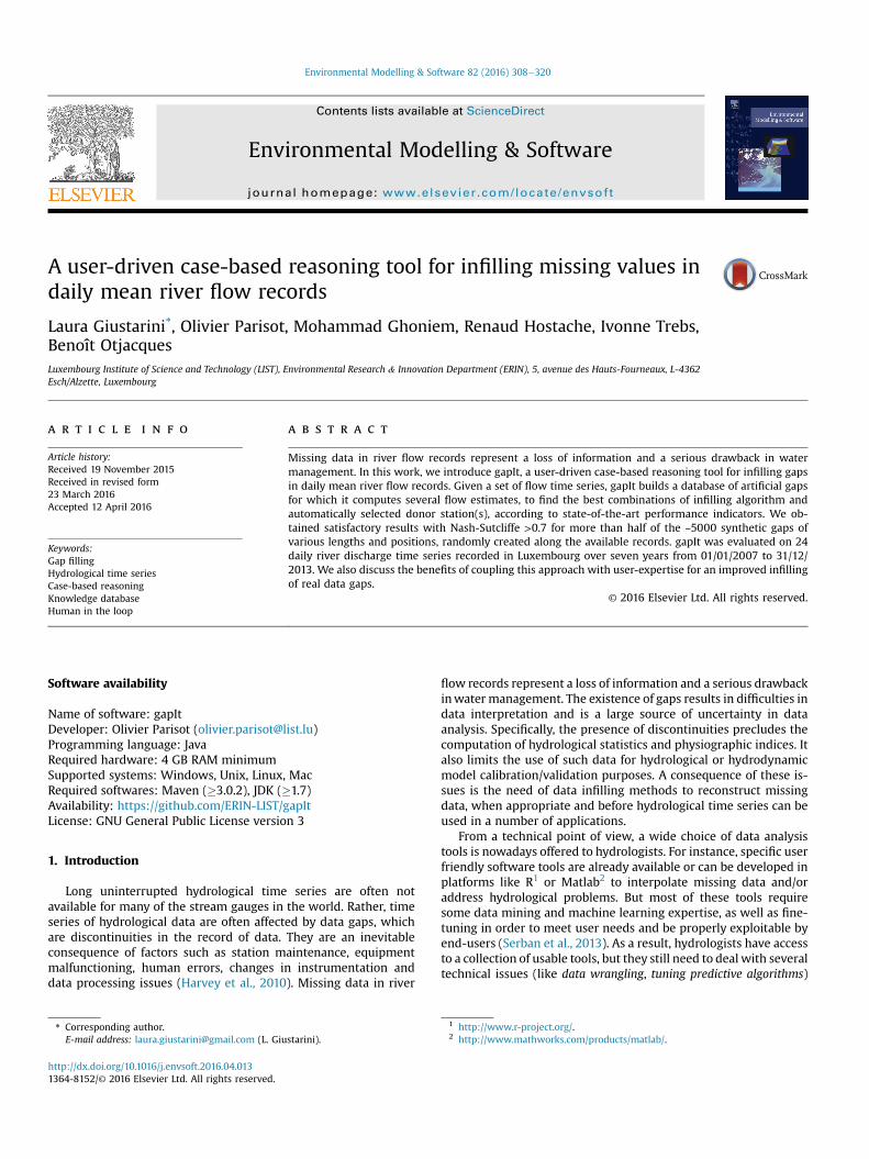
number of infilling methods. For each bin, we divided the numberof best solutions by the total number of best solutions, i.e. 5108, toobtain the percentage.

Fig. 8 shows the distribution of best solutions across all infillingmethods, regardless of the number/type of donor stations and gaplengths. Under these conditions, ANN and MT were found to be themost accurate methods for infilling the majority of the syntheticgaps, with low MAE and RMSE values and high NS coefficients.

A similar trend to that displayed in Fig. 8 has been observedwithseasonal gaps. When clustering by flow regimes, the percentages ofselected methods are comparable to what was found for the totalnumber of gaps. Interestingly, however, INTERP was never selectedto infill gaps in high flow condition, while it was chosen for infilling1% and 8% of middle and low flow regime gaps, respectively. Thiscan be explained by the fact that low flow conditions tend to showless important discharge variations, while in case of a flood event, arapid increase and/or decrease of values is usually observed.

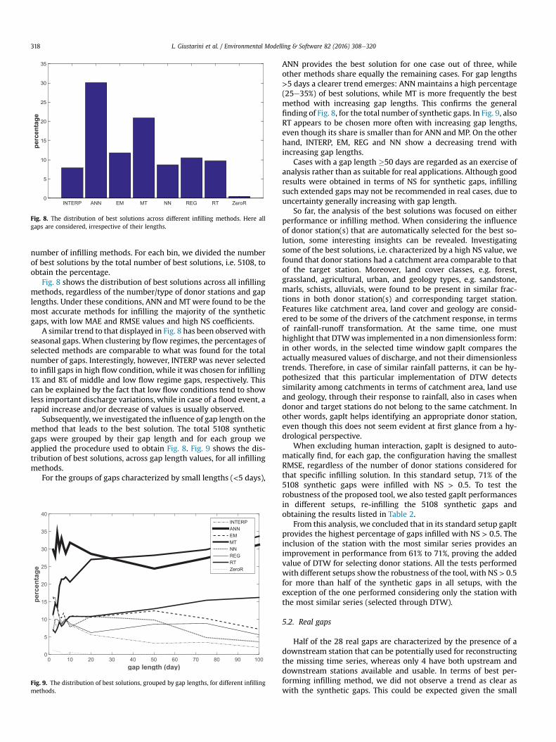
Subsequently, we investigated the influence of gap length on themethod that leads to the best solution. The total 5108 syntheticgaps were grouped by their gap length and for each group weapplied the procedure used to obtain Fig. 8. Fig. 9 shows the dis-tribution of best solutions, across gap length values, for all infillingmethods.

For the groups of gaps characterized by small lengths (<5 days),

gap length (day)

0 10 20 30 40 50 60 70 80 90 100

percen

tag

e

0

5

10

15

20

25

30

35

40INTERPANNEMMTNNREGRTZeroR

Fig. 9. The distribution of best solutions, grouped by gap lengths, for different infillingmethods.

ANN provides the best solution for one case out of three, whileother methods share equally the remaining cases. For gap lengths>5 days a clearer trend emerges: ANN maintains a high percentage(25e35%) of best solutions, while MT is more frequently the bestmethod with increasing gap lengths. This confirms the generalfinding of Fig. 8, for the total number of synthetic gaps. In Fig. 9, alsoRT appears to be chosen more often with increasing gap lengths,even though its share is smaller than for ANN and MP. On the otherhand, INTERP, EM, REG and NN show a decreasing trend withincreasing gap lengths.

Cases with a gap length �50 days are regarded as an exercise ofanalysis rather than as suitable for real applications. Although goodresults were obtained in terms of NS for synthetic gaps, infillingsuch extended gaps may not be recommended in real cases, due touncertainty generally increasing with gap length.

So far, the analysis of the best solutions was focused on eitherperformance or infilling method. When considering the influenceof donor station(s) that are automatically selected for the best so-lution, some interesting insights can be revealed. Investigatingsome of the best solutions, i.e. characterized by a high NS value, wefound that donor stations had a catchment area comparable to thatof the target station. Moreover, land cover classes, e.g. forest,grassland, agricultural, urban, and geology types, e.g. sandstone,marls, schists, alluvials, were found to be present in similar frac-tions in both donor station(s) and corresponding target station.Features like catchment area, land cover and geology are consid-ered to be some of the drivers of the catchment response, in termsof rainfall-runoff transformation. At the same time, one musthighlight that DTWwas implemented in a non dimensionless form:in other words, in the selected time window gapIt compares theactually measured values of discharge, and not their dimensionlesstrends. Therefore, in case of similar rainfall patterns, it can be hy-pothesized that this particular implementation of DTW detectssimilarity among catchments in terms of catchment area, land useand geology, through their response to rainfall, also in cases whendonor and target stations do not belong to the same catchment. Inother words, gapIt helps identifying an appropriate donor station,even though this does not seem evident at first glance from a hy-drological perspective.

When excluding human interaction, gapIt is designed to auto-matically find, for each gap, the configuration having the smallestRMSE, regardless of the number of donor stations considered forthat specific infilling solution. In this standard setup, 71% of the5108 synthetic gaps were infilled with NS > 0.5. To test therobustness of the proposed tool, we also tested gapIt performancesin different setups, re-infilling the 5108 synthetic gaps andobtaining the results listed in Table 2.

From this analysis, we concluded that in its standard setup gapItprovides the highest percentage of gaps infilled with NS > 0.5. Theinclusion of the station with the most similar series provides animprovement in performance from 61% to 71%, proving the addedvalue of DTW for selecting donor stations. All the tests performedwith different setups show the robustness of the tool, with NS > 0.5for more than half of the synthetic gaps in all setups, with theexception of the one performed considering only the station withthe most similar series (selected through DTW).

5.2. Real gaps

Half of the 28 real gaps are characterized by the presence of adownstream station that can be potentially used for reconstructingthe missing time series, whereas only 4 have both upstream anddownstream stations available and usable. In terms of best per-forming infilling method, we did not observe a trend as clear aswith the synthetic gaps. This could be expected given the small

Table 2Comparison of different setups.

Setup Gaps infilled with NS > 0.5

Standard setup 71%Standard setup but excluding the station with the most similar series 61%Using only the station with the most similar series 44%Using the station with the most similar series and the geographically closest one 58%

L. Giustarini et al. / Environmental Modelling & Software 82 (2016) 308e320 319

number of cases. However, it is interesting to report that MT wasthe top performer in 8 cases, while EM was never selected.

To assess the quality of infilling, performance measures werecomputed according to Evaluation strategy B. Out of the 28 realgaps, 19 achieved an NS coefficient >0.8. As mentioned before, thiscan be only regarded a simple hint and not as a real performancevalue. For instance, in an extreme case, a peak discharge may haveoccurred, due to localized rainfall, only in a limited area and it alsomay have been recorded (potentially) by only a single station,whereas all other stations in the surrounding region are notaffected by rainfall and, hence, do not detect any particulardischarge variation. In case the first station would be affected by adata gap, exactly during that flood event, none of the proposedinfilling methods would be able to correctly reconstruct it. How-ever, the performance indicators would be quite high, indicatinggood infilling results. This highlights the importance of combiningautomatic techniques with user expertise and knowledge, asimplemented in gapIt, to obtain reliable gap infilling results.

6. Conclusions

In this paper, we presented gapIt, a tool for infilling gaps inhydrological discharge time series.

It was tested in the gauging network of Luxembourg to performgap infilling on daily values, leading to satisfactory results onsynthetic gaps. The tool was used for infilling ~5000 synthetic gaps,of different lengths and positions, randomly created along theentire records of all stations. More than half of the synthetic gapswere reconstructed with NS > 0.7. The software showed stableperformance, regardless of gap length and flow regime. Superiorperformance was obtained by the use of methods such as neuralnetworks and regression trees. Subsequently, gapIt was applied toinfill 28 real gaps, ranging in length from 2 to 95 days. The goodperformance values obtained for more than half of them need to beconsidered as simple hints, as it is precisely in these situations thatthe added value of gapIt is revealed, consisting in combining anautomated data-driven approach with the interactive user-drivenrefinements based on domain expertise through the visual in-spection of the proposed solutions in their spatio-temporal context.

The proposed gapIt software provides a framework for a morestandardized and traceable gap infilling process. The solutionreached for infilling any specific gap can be retrieved for futureanalysis, while the infilled data are appropriately flagged. Ideally,the infilled data should also be characterized with an estimate ofuncertainty. If the infilling is then used to calibrate or validatemodels, such uncertainty can be taken into account: that wouldcomply with the good practice also suggested by Beven (2015). Aproper uncertainty analysis should distinguish between any un-certainty deriving, for instance, from measurement instrumentsthemselves, poor rating curves, etc., and uncertainty introduced bythe infilling procedure. In the present case study, the uncertainty ofthe infilled data would derive partially from the uncertain data(discharge values computed through uncertain rating curves) usedto reconstruct them and partially from the uncertainty inherent inthe infilling method adopted. Futureworkwill focus on uncertaintyanalysis, disentangling the different components of uncertainty

(Beven and Westerberg, 2011), to better deal with the risks ofinjecting, through infilling, disinformative or inconsistent values.

In its current setup, the main advantage of the software is that itoffers the opportunity of taking the best advantage of softwareautomation and human expertise. When the user encounters a realgap, gapIt may help find the best possible solution through CBR.Nevertheless, the user can always modify both the proposedinfilling method and/or the set of donor stations. In fact, a databaseof infilled synthetic gaps is available from the start in gapIt andfrom there the tool can suggest the best solution. However, anysolution obtained for a real gap by an expert working with this toolis added to the database, indirectly including part of the humanexpertise into the database itself. The more cases are stored in thesystem, the better results it will achieve.

It is important to note that at present no limit for the distancebetween target and donor station was set. This is a consequence ofthe limited area of our case study. However, when dealing withlarger regions, it is legitimate to foresee the application of spatiallimits in the search for donor station(s). These limits may be setaccording to the knowledge of the hydraulic and hydrologicalbehavior of the region and should probably be different from sta-tion to station. Like most CBR systems, gapIt will always provide asolution, regardless of the number of similar cases available, or thestrength of the similarity. For example, if all donor stations exceptone havemissing data in the same time period as the target station,the algorithm will use that single station as donor, as it is the onlyone available with recorded data, regardless of its location in spaceand/or its similarity in terms of DTW. This could be an issue inlarger regions with several periods of instrument malfunctioning.Coupling the automatic algorithm with the visual inspection toolwill allow the user to compensate the unavoidable drawbacks of apurely data-driven approach.

First promising results were obtained infilling 15-min values(i.e. original resolution of the present case study). However, due tothe complexity of dealing with high frequency sampling, furthertesting is needed. Despite its versatility and capability of workingwith different temporal resolutions, in the present implementationgapIt cannot deal with irregularly sampled data and/or very sparsemeasurement networks, where the need for infilling is arguablymore critical.

Acknowledgements

This study was funded by the Luxembourg Institute of Scienceand Technology (LIST). We are grateful to the anonymous reviewersfor their valuable comments and suggestions to improve the paper.

References

Aamodt, A., Plaza, E., 1994. Case-based reasoning: foundational issues, methodo-logical variations, and system approaches. AI Commun. 7 (1), 39e59.

Bennis, S., Berrada, F., Kang, N., 1997. Improving single-variable and multivariabletechniques for estimating missing hydrological data. J. Hydrol. 191 (1), 87e105.

Berndt, D.J., Clifford, J., 1994. Using dynamic time warping to find patterns in timeseries. In: KDD Workshop’94, pp. 359e370.

Beven, K., 2015. Facets of uncertainty: epistemic uncertainty, non-stationarity,likelihood, hypothesis testing, and communication. Hydrol. Sci. J. http://dx.doi.org/10.1080/02626667.2015.1031761.

L. Giustarini et al. / Environmental Modelling & Software 82 (2016) 308e320320

Beven, K., Smith, P., 2014. Concepts of information content and likelihood inparameter calibration for hydrological simulation models. J. Hydrol. Eng. 20.

Beven, K., Westerberg, I., 2011. On red herrings and real herrings: disinformationand information in hydrological inference. Hydrol. Process. 25, 1676e1680.

Breunig, M.M., Kriegel, H.-P., Ng, R.T., Sander, J., 2000. Lof: identifying density-basedlocal outliers. In: ACM Sigmod Record, vol. 29. ACM, pp. 93e104.

Croke, B., 2006. A technique for deriving an average event unit hydrograph fromstreamflow-only data for ephemeral quick-flow-dominant carchments. Adv.Water Resour. 29, 493e502.

Didry, Y., Parisot, O., Tamisier, T., 2015. Engineering data intensive applications withcadral. In: Cooperative Design, Visualization, and Engineering: 12th Interna-tional Conference, CDVE 2015, Mallorca, Spain, September 20-23, 2015. Pro-ceedings. Springer.

Domingos, P., 2012. A few useful things to know about machine learning. Commun.ACM 55 (10), 78e87.

Enders, C.K., 2010. Applied Missing Data Analysis. Guilford Publications.F�eraud, R., Cl�erot, F., 2002. A methodology to explain neural network classification.

Neural Netw. Off. J. Int. Neural Netw. Soc. 15 (2), 237e246.Gao, C., Yao, M., Wang, Y., Zhai, J., Buda, S., Fischer, T., Zeng, X., Wang, W., 2015.

Hydrological model comparison and assessment: criteria from catchment scalesand temporal resolution. Hydrol. Sci. J. http://dx.doi.org/10.1080/02626667.2015.1057141.

Gilbert, D., 2002. The Jfreechart Class Library. Developer Guide. Object Refinery 7.Griffioen, J., Vermooten, S., Kukuric, N., Vasak, S., Demuth, S., Gustard, A., Planos, E.,

Seatena, F., Servat, E., et al., 2006. A european case-based reasoning tool tointer-compare hydrological information on water stress among drainage sub-basins. Clim. Var. Change Hydrol. Impacts 91e96.

Gyau-Boakye, P., Schultz, G., 1994. Filling gaps in runoff time series in West Africa.Hydrol. Sci. J. 39 (6), 621e636.

Harmal, R., Smith, P., Migliaccio, K., Chaubex, I., Douglas-Mankin, K., Benham, B.,Shukla, S.,R.,M.-C., Robson, B., 2014. Evaluating, interpreting, and communi-cating performance of hydrologic/water quality models considering intendeduse: a review and recommendations. Environ. Model. Softw. 57, 40e51.

Harvey, C.L., Dixon, H., Hannaford, J., 2010. Developing best practice for infillingdaily river flow data. Role Hydrol. Manag. Consequences a Chang. Glob. Environ.816e823.

Harvey, C.L., Dixon, H., Hannaford, J., 2012. An appraisal of the performance of data-infilling methods for application to daily mean river flow records in the UK.Hydrol. Res. 43 (5), 618e636.

Johnston, C.A., 1999. Development and Evaluation of Infilling Methods for MissingHydrologic and Chemical Watershed Monitoring Data. Ph.D. thesis. VirginiaPolytechnic Institute and State University.

Junninen, H., Niska, H., Tuppurainen, K., Ruuskanen, J., Kolehmainen, M., 2004.Methods for imputation of missing values in air quality data sets. Atmos. En-viron. 38 (18), 2895e2907.

Kirchner, J., 2009. Catchments as simple dynamical systems: catchment charac-terization, rainfall-runoff modeling, and doing hydrology backward. WaterResour. Res. 45.

Kotsiantis, S., 2013. Decision trees: a recent overview. Artif. Intell. Rev. 39 (4),261e283.

Krause, P., Boyle, D., Bsw, F., 2005. Comparison of different efficiency criteria forhydrological model assessment. Adv. Geosci. 5, 78e97.

Kretzschmar, A., Tych, W., Chappell, N., 2014. Reversing hydrology: estimation ofsub-hourly rainfall time-series from streamflow. Environ. Model. Softw. 60,290e301.

Legates, D., McCabe Jr., G., 1999. Evaluating the use of “goodness-of-fit” measures inhyfrologic and hydroclimatic model validation. Water Resour. Res. 35, 233e241.

Maimon, O.Z., Rokach, L., 2005. Data Mining and Knowledge Discovery Handbook,vol. 1. Springer.

Marwala, T., Global, I., 2009. Computational Intelligence for Missing Data Imputa-tion, Estimation and Management: Knowledge Optimization Techniques. In-formation Science Reference Herhsey, USA.

Matthies, M., Giupponi, C., Ostendorf, B., 2007. Environmental decision supportsystems: current issues, methods and tools. Environ. Model. Softw. 22 (2),123e127.

Moriasi, D.N., Arnold, J.G., Van Liew, M.W., Bingner, R.L., Harmel, R.D., Veith, T.L.,2007a. Model evaluation guidelines for systematic quantification of accuracy inwatershed simulations. Trans. ASABE 50 (3), 885e900.

Moriasi, D., Arnold, J., Van Liew, M., Bingner, R., Harmel, R., Veith, T., 2007b. Modelevaluation guidelines for systematic quantification of accuracy in watershedsimulations. Trans. Asabe 50 (3), 885e900.

Mwale, F., Adeloye, A., Rustum, R., 2012. Infilling of missing rainfall and streamflowdata in the shire river basin, malawiea self organizing map approach. Phys.Chem. Earth Parts A/B/C 50, 34e43.

Nash, J., Sutcliffe, J., 1970. River flow forecasting through conceptual models part i adiscussion of principles. J. Hydrol. 10 (3), 282e290.

Ouyang, R., Ren, L., Cheng, W., Zhou, C., 2010. Similarity search and pattern dis-covery in hydrological time series data mining. Hydrol. Process. 24 (9),1198e1210.

Pigott, T.D., 2001. A review of methods for missing data. Educ. Res. Eval. 7 (4),353e383.

Quinlan, J.R., 1992. Learning with continuous classes. In: Proceedings of the 5thAustralian Joint Conference on Artificial Intelligence. Vol. 92. Singapore,pp. 343e348.

Salas, J.D., 1980. Applied Modeling of Hydrologic Time Series. Water ResourcesPublication.

Sattari, M.T., Pal, M., Apaydin, H., Ozturk, F., 2013. M5 model tree application in dailyriver flow forecasting in sohu stream, Turkey. Water Resour. 40 (3), 233e242.

Serban, F., Vanschoren, J., Kietz, J.-U., Bernstein, A., 2013. A survey of intelligentassistants for data analysis. ACM Comput. Surv. (CSUR) 45 (3), 31.

Tfwala, S.S., Wang, Y.-M., Lin, Y.-C., 2013. Prediction of missing flow records usingmultilayer perceptron and coactive neurofuzzy inference system. Sci. World J.2013. Article ID 584516, 7 pages, http://dx.doi.org/10.1155/2013/584516.

Van Buuren, S., 2012. Flexible Imputation of Missing Data. Chapman & Hall/CRC.Interdisciplinary Statistics.

Van Hulse, J., Khoshgoftaar, T.M., 2008. A comprehensive empirical evaluation ofmissing value imputation in noisy software measurement data. J. Syst. Softw. 81(5), 691e708.

Witten, I.H., Frank, E., Hall, M.A., 2011. Data Mining: Practical Machine LearningTools and Teechniques. Elsevier.

Wrede, S., Fenicia, F., Martnez-Carreras, N., Juilleret, J., Hissler, C., Krein, A.,Savenije, H., Uhlenbrook, S., Kavetski, D., Pfister, L., 2015. Towards more sys-tematic perceptual model development: a case study using 3 luxembourgishcatchments. Hydrol. Process. 29 (12), 2731e2750.