a university of michigan library instructional technology ... · getting started with excel 2010 a...

Getting Started with Excel 2010 A University of Michigan Library Instructional Technology Workshop

Need help? Visit the Faculty Exploratory or Knowledge Navigation Center on the 2nd floor of the Graduate Library.

[email protected] | http://www.lib.umich.edu/guides | [email protected]

rev: 8/3/11

1 of 17

Table of Contents

Introduction ................................................................................................................... 2

New Tools ...................................................................................................................................................... 2

Elements of An Excel Document ................................................................................. 3

Resizing and Hiding Columns and Rows .................................................................................................. 3

Using Panes to Create Spreadsheet Headers ............................................................................................. 4

Page Break Preview ....................................................................................................................................... 4

Using the AutoFill Command ....................................................................................... 5

Using AutoFill for Sequences ...................................................................................................................... 5

Using AutoFill for Formulas ....................................................................................................................... 5

Using Formulas and Functions ..................................................................................... 6

Using the AutoSum Command ................................................................................................................... 6

Inserting a Function ...................................................................................................................................... 7

Creating Weighted Averages Exercise ....................................................................... 8

Defining a Named Area ............................................................................................................................... 9

Using the Named Area in a Formula ......................................................................................................... 9

Substituting Letter Grades Exercise ........................................................................... 10

COUNTIF Exercise ........................................................................................................ 12

TRIM Exercise ............................................................................................................... 12

Formatting .................................................................................................................... 13

Cells, Columns and Rows .......................................................................................................................... 13

Formatting Your Worksheet ..................................................................................................................... 13

Sorting Data ................................................................................................................. 14

Filtering Data................................................................................................................ 15

Advanced Filter ........................................................................................................................................... 15

Adding A Chart ........................................................................................................... 16

Modifying ..................................................................................................................................................... 16

Working with Pivot Tables ........................................................................................... 17

Selecting the Data ........................................................................................................................................ 17

Creating the Report ..................................................................................................................................... 17




rev: 8/3/11

2 of 17

INTRODUCTION Although Microsoft Office 2010 looks very similar to Office 2007, there are a couple of changes. One of the changes is that the Office Button has become the File Ribbon in Office 2010. The File Ribbon contains such standard features as Open, Close, Print, Save, etc. In addition, this menu allows you to quickly manage Word settings (Permissions, Sharing ,Versions, Properties, and Options).

NEW TOOLS

Preview data before you paste: Copy your original data, click the cell you would like to paste into, go to the Home Ribbon, and click the arrow below the Paste icon and hover over a button to preview your data. Click the button to paste the data.

Inserting screen shots: In the Insert Ribbon, there is now a Screenshot icon

( ) in the Illustrations Group. You can insert a screenshot of any open window on your screen, or you can choose a specific part of your screen (Screen Clipping) to insert.




rev: 8/3/11

3 of 17

ELEMENTS OF AN EXCEL DOCUMENT When you open Excel, a blank workbook is automatically opened. A workbook is a file with one or more sheets; each worksheet (sometimes called spreadsheet) is a “page” in the workbook where you enter and work with your data. Each workbook starts with three sheets, but you can add more by clicking on the Insert Worksheet icon to the right of your last sheet‟s tab (circled below). To change the name, double-click on the sheet‟s tab and then type the new name.

An Excel worksheet is made up of a series of columns (named with letters e.g. A, B, C…) and rows (named with numbers e.g. 1, 2, 3…) that define the cells – for example, “C3”. To enter data (text or numbers), click in the appropriate cell and start typing. When you type, the data goes into the currently selected cell, called the active cell. All the data you enter in the active cell appears in the Formula bar. If you need to change the data, you can double-click on the cell to activate the cursor in the cell, or click in the Formula bar and make the change there.

To navigate more quickly in your worksheet, use the arrow keys on the keyboard to move left, right, up and down. In addition, you can use the following other keystrokes:

Enter accepts your entry and moves the active cell down one; hold down the Shift key as well and you will move back up.

Tab accepts your entry and moves the active cell to the right. Again, hold down the Shift key as well as the Tab key and you will move to the left.

The Esc key or red X in the Formula bar will abort your change.

RESIZING AND HIDING COLUMNS AND ROWS You can change a column‟s width by putting your cursor between the letter for that column and the next (between A and B at right). When you get the two-headed arrow, drag to the right or left as desired.

Double-clicking on that same spot will “autofit” the column, making the column as wide as the largest piece of text/data in that column.

The same technique works for rows; put your cursor between the two numbers until you see the two-headed arrow, and then drag or double-click.

Active Cell




rev: 8/3/11

4 of 17

To hide a column or row, right-click on the letter or number for the column or row (A, B, C, etc. or 1, 2, 3, etc.) and select Hide. To unhide a column or row, select the columns or rows before and after the missing column or row, right-click, and select Unhide.

For exact height or width control (or to hide a row or column), go to the Cells Group in the Home Ribbon then click the arrow below the Format icon.

USING PANES TO CREATE SPREADSHEET HEADERS If your data set is large and it is difficult to see which values correspond to what heading, you can make the top rows and leftmost columns into headers that will stay put at the top and left as you scroll around the page.

You can “lock” the first column or the top row in place by going to the View Ribbon, click on the Freeze Panes icon in the Window Group, and choosing either Freeze Top Row or Freeze First Column (you would have to do this one at a time if you wanted to freeze them both). To unfreeze either, go back to the same place, and it will now say “unfreeze”.

If you click the Split icon (still in the Window Group), it will add a horizontal and vertical split in your document that you can adjust, and then freeze. You can also drag the panes into position:

1. At the top of the vertical scroll bar, there is a thick bar. Move your cursor over this bar and it changes to two parallel lines with an arrow.

2. Click and drag to divide the window vertically into panes. Adjust the split so that the first row (or two) is the only row in the top pane.

3. To set a horizontal pane, use the similar thick bar at the lower right corner of the scroll bar and drag it to the left.

To freeze the panes in place, go to the View Ribbon, click on the Freeze Panes icon in the Window Group, and choose Freeze Panes. Note, you don‟t have to set them both; you can use just the vertical or just the horizontal. Once you freeze the panes, however, you need to unfreeze them to either adjust them or add another pane.

To remove the pane(s), click on the Freeze Panes icon in the Window Group, and choose Unfreeze Pane.

Once you have the column and row headings in place, you can scroll left to right and top to bottom and they will remain in place. This can be very useful to manipulate your data – see the Sorting Data section on page 14 for more information.

PAGE BREAK PREVIEW To see where your data will split into multiple pages, go to the View Ribbon and click Page Break Preview icon in the Workbook Views Group. Adjust the page breaks by clicking and dragging the blue borders with your mouse. To return to the normal view, click on the Normal icon.




rev: 8/3/11

5 of 17

USING THE AUTOFILL COMMAND Excel has a feature that helps you automatically enter data. If you are entering a predictable series (e.g. 1, 2, 3…; days of the week; hours of the day) you can use the AutoFill command to automatically extend the sequence. You can also use this for formulas – set up the formula once, then use the AutoFill to propagate it to the other cells.

USING AUTOFILL FOR SEQUENCES For Excel to know how to fill in the series, you usually need to provide two or three examples. In the case of months, weekdays, and hours, you only need to provide one example.

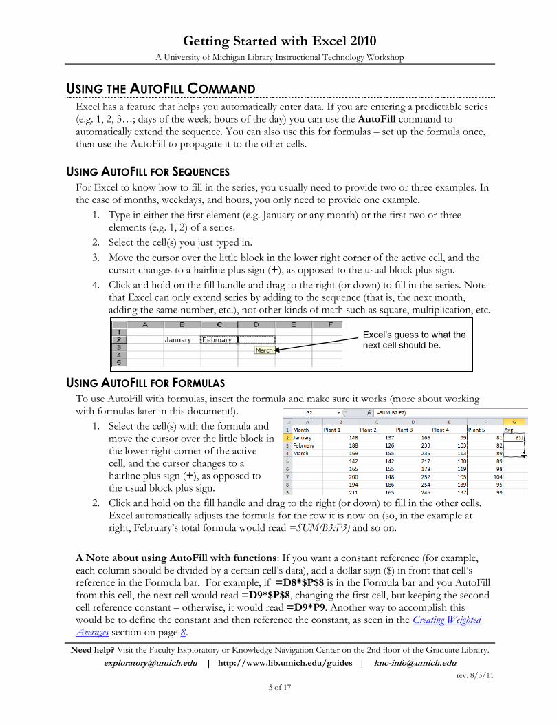
1. Type in either the first element (e.g. January or any month) or the first two or three elements (e.g. 1, 2) of a series.

2. Select the cell(s) you just typed in.

3. Move the cursor over the little block in the lower right corner of the active cell, and the cursor changes to a hairline plus sign (+), as opposed to the usual block plus sign.

4. Click and hold on the fill handle and drag to the right (or down) to fill in the series. Note that Excel can only extend series by adding to the sequence (that is, the next month, adding the same number, etc.), not other kinds of math such as square, multiplication, etc.

USING AUTOFILL FOR FORMULAS To use AutoFill with formulas, insert the formula and make sure it works (more about working with formulas later in this document!).

1. Select the cell(s) with the formula and move the cursor over the little block in the lower right corner of the active cell, and the cursor changes to a hairline plus sign (+), as opposed to the usual block plus sign.

2. Click and hold on the fill handle and drag to the right (or down) to fill in the other cells. Excel automatically adjusts the formula for the row it is now on (so, in the example at right, February‟s total formula would read =SUM(B3:F3) and so on.

A Note about using AutoFill with functions: If you want a constant reference (for example, each column should be divided by a certain cell‟s data), add a dollar sign ($) in front that cell‟s reference in the Formula bar. For example, if =D8*$P$8 is in the Formula bar and you AutoFill from this cell, the next cell would read =D9*$P$8, changing the first cell, but keeping the second cell reference constant – otherwise, it would read =D9*P9. Another way to accomplish this would be to define the constant and then reference the constant, as seen in the Creating Weighted Averages section on page 8.

Excel’s guess to what the next cell should be.




rev: 8/3/11

6 of 17

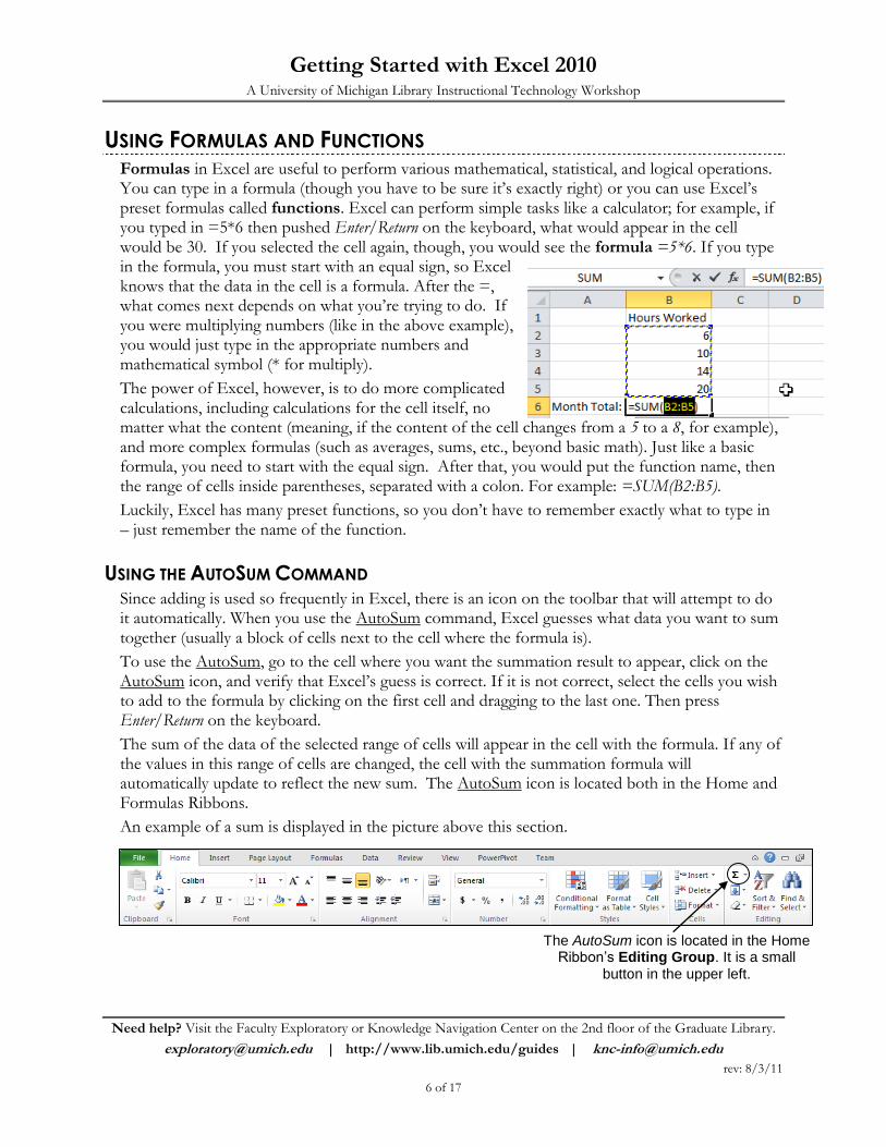
USING FORMULAS AND FUNCTIONS Formulas in Excel are useful to perform various mathematical, statistical, and logical operations. You can type in a formula (though you have to be sure it‟s exactly right) or you can use Excel‟s preset formulas called functions. Excel can perform simple tasks like a calculator; for example, if you typed in =5*6 then pushed Enter/Return on the keyboard, what would appear in the cell would be 30. If you selected the cell again, though, you would see the formula =5*6. If you type in the formula, you must start with an equal sign, so Excel knows that the data in the cell is a formula. After the =, what comes next depends on what you‟re trying to do. If you were multiplying numbers (like in the above example), you would just type in the appropriate numbers and mathematical symbol (* for multiply).

The power of Excel, however, is to do more complicated calculations, including calculations for the cell itself, no matter what the content (meaning, if the content of the cell changes from a 5 to a 8, for example), and more complex formulas (such as averages, sums, etc., beyond basic math). Just like a basic formula, you need to start with the equal sign. After that, you would put the function name, then the range of cells inside parentheses, separated with a colon. For example: =SUM(B2:B5).

Luckily, Excel has many preset functions, so you don‟t have to remember exactly what to type in – just remember the name of the function.

USING THE AUTOSUM COMMAND Since adding is used so frequently in Excel, there is an icon on the toolbar that will attempt to do it automatically. When you use the AutoSum command, Excel guesses what data you want to sum together (usually a block of cells next to the cell where the formula is).

To use the AutoSum, go to the cell where you want the summation result to appear, click on the AutoSum icon, and verify that Excel‟s guess is correct. If it is not correct, select the cells you wish to add to the formula by clicking on the first cell and dragging to the last one. Then press Enter/Return on the keyboard.

The sum of the data of the selected range of cells will appear in the cell with the formula. If any of the values in this range of cells are changed, the cell with the summation formula will automatically update to reflect the new sum. The AutoSum icon is located both in the Home and Formulas Ribbons.

An example of a sum is displayed in the picture above this section.

The AutoSum icon is located in the Home Ribbon’s Editing Group. It is a small

button in the upper left.




rev: 8/3/11

7 of 17

INSERTING A FUNCTION There are several ways to insert functions. Before anything, you need to make sure your cursor is in the cell in which you want the result. Once there, choose one of the methods below to insert your function:

On the Home Ribbon, click on the arrow next to the AutoSum icon and select More Functions…

Go to the Formulas Ribbon – choose either the Insert Function icon to bring up the Insert Function dialog box (same dialog box you would get with the first method), or click the arrow next to the correct category in the Function Library Group, and then choose the exact function.

If you choose More Functions… from the Home Ribbon or the Insert Function icon on the Formulas Ribbon, you will see the Insert Function dialog box. The Insert Function dialog box gives you a list of operations that Excel can perform.

Choose a category from the Select a category: pulldown (which includes an option to show all), and then a particular function from the Select a function: pulldown.

Another dialog box opens which asks you to select the cells you would like to involve in the formula. To select, use the mouse to click on the first cell and drag through the cells you would like to add. Note that for each function, this second window will look different.

If you‟re not sure how to use a particular function, you can click the Help on this function link in the Insert Function dialog box, and that will bring up Excel‟s Help.

Once the function is in the cell, you can copy and then paste it into another cell to do the same function for that different range of cells. You can also use the AutoFill command (click cell with the function, then drag to the right or down). The formula adjusts automatically for the new values.

As mentioned before, if you want a constant reference (for example, each column should be divided by a certain cell‟s data), add a dollar sign ($) in front that cell‟s reference in the Formula bar. For example, if =D8*$P$8 is in the Formula bar and you AutoFill from this cell, the next cell would read =D9*$P$8, changing the first cell, but keeping the second cell reference constant – otherwise, it would read =D9*P9. Another way to accomplish this would be to define the constant and then reference the constant, as seen below in the Creating Weighted Averages section.

There are so many different functions in Excel that it would be difficult to cover them all, but we will include a few below in addition to the AutoSum that was explained above on page 6.




rev: 8/3/11

8 of 17

Quick Reference: 1. Enter weights 2. Select cells and name weights 3. Insert the sumproduct function

a. Array 1 = first student’s scores b. Array 2 = Weights

4. Click OK and AutoFill

CREATING WEIGHTED AVERAGES EXERCISE Suppose the final exam is 50% of the grade, and the homework and midterm are 25% each. To make a weighted average, each score is multiplied by the decimal equivalent of its weight, and the weighted scores are added up. The only restriction on a weighted average is that the weights must sum to 1 (or 100%). You could type this in by hand, for example: =0.25*q3+0.25*r3+0.5*s3 but the problem with that is you would have to get into each cell to make the change if you need to alter the weights for a different semester or class.

Excel has a function called sumproduct, which adds the products within a range of cells, so by using that function, we can avoid having to type in all that in the example above. In addition, because functions can refer to cell contents – and thereby change as the cell content changes – we use the cell references for our weights, and so if they change, our formula results will automatically changes. For example, if the weights change (so the final exam is now worth 40%, and the midterm and homework are now 30% each), as long as the cells themselves are referenced (rather than the specific numeric value), the formula will automatically update.

If we add the weights above each column heading, insert the sumproduct function, choose the student‟s scores (Array1) and then the weights (Array2), the formula will be correct for the first student. If we try to use the AutoFill command, however, as we discussed in the Using AutoFill for Formulas on page 5, both cell references will moved down – so the second student‟s formula would be incorrect (as shown at right).

We can either use the $ (dollar sign) to “lock in” the cell references for the weights, or we can define a named area referencing the cells with the weight information, and then use that name in the formula to reference those cells.

Before we start, create a new column for the weighted averages for all of the students. This way we can compare the weighted averages with the non-weighted averages.




rev: 8/3/11

9 of 17

DEFINING A NAMED AREA 1. Enter a set of weights for each score at the top or bottom of each grade column (e.g. .25,

.25, .50). Make sure the weighting adds up to 1.

2. Select the cells containing the weights.

3. In the Formula Ribbon, go to the Defined Names Group and click on the Define Name icon.

4. In the New Name dialog box, type a name in the Name: field – note, Excel may guess at a name if an adjacent cell seems to be the label.

5. If you‟ve already selected the cells (as we suggested in step 2), the Refers To: field will already have the correct cell information.

6. Click OK to accept the name for these cells – in our example here, “Weights”.

USING THE NAMED AREA IN A FORMULA In the Weighted Score column you created, click in the empty cell for the first student‟s score. To insert the sumproduct function,

1. Go to the Formulas Ribbon, click on the arrow next to the Math&Trig icon in the Function Library Group, and choose SUMPRODUCT.

2. Select the cells with the first student‟s scores for Array1.

3. Type in the name Weights (or whatever you called it) in Array2. Note this field is case-sensitive - you‟ll know you have it correct with the contents of the cells displays next to the field, and the result will display in the lower right of the dialog box.

4. Click OK to exit the dialog box.

5. Use the fill handle to extend the formula to all students.




rev: 8/3/11

10 of 17

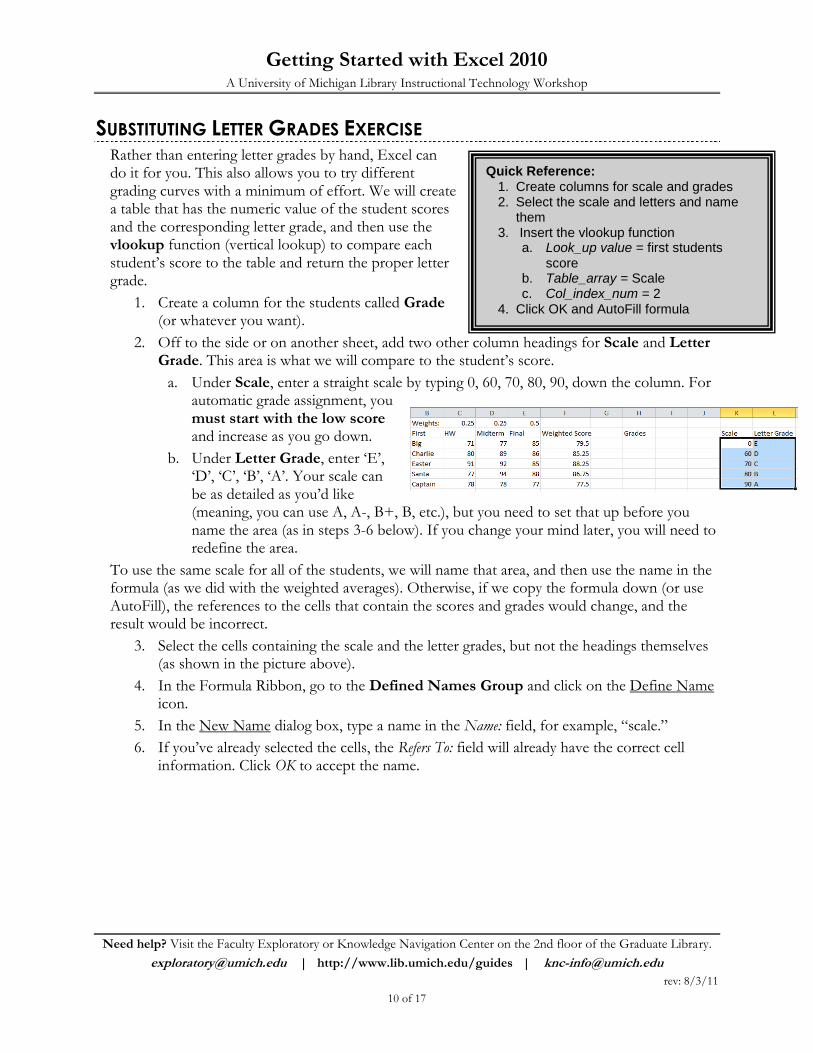
Quick Reference: 1. Create columns for scale and grades 2. Select the scale and letters and name

them 3. Insert the vlookup function

a. Look_up value = first students score

b. Table_array = Scale c. Col_index_num = 2

4. Click OK and AutoFill formula

SUBSTITUTING LETTER GRADES EXERCISE Rather than entering letter grades by hand, Excel can do it for you. This also allows you to try different grading curves with a minimum of effort. We will create a table that has the numeric value of the student scores and the corresponding letter grade, and then use the vlookup function (vertical lookup) to compare each student‟s score to the table and return the proper letter grade.

1. Create a column for the students called Grade (or whatever you want).

2. Off to the side or on another sheet, add two other column headings for Scale and Letter Grade. This area is what we will compare to the student‟s score.

a. Under Scale, enter a straight scale by typing 0, 60, 70, 80, 90, down the column. For automatic grade assignment, you must start with the low score and increase as you go down.

b. Under Letter Grade, enter „E‟, „D‟, „C‟, „B‟, „A‟. Your scale can be as detailed as you‟d like (meaning, you can use A, A-, B+, B, etc.), but you need to set that up before you name the area (as in steps 3-6 below). If you change your mind later, you will need to redefine the area.

To use the same scale for all of the students, we will name that area, and then use the name in the formula (as we did with the weighted averages). Otherwise, if we copy the formula down (or use AutoFill), the references to the cells that contain the scores and grades would change, and the result would be incorrect.

3. Select the cells containing the scale and the letter grades, but not the headings themselves (as shown in the picture above).

4. In the Formula Ribbon, go to the Defined Names Group and click on the Define Name icon.

5. In the New Name dialog box, type a name in the Name: field, for example, “scale.”

6. If you‟ve already selected the cells, the Refers To: field will already have the correct cell information. Click OK to accept the name.




rev: 8/3/11

11 of 17

Now we‟re ready to use that newly named area to assign grades. The vlookup function looks up a value in the first column of a table (where the values in the first column are increasing) and returns the value in any other column of the table.

In our case, then, we will compare the student‟s weighted score to the first column of the table (our scale) and return the value in the second column (the letter grade). Because we have defined this area with a name, if we change the scale to grade on a curve (so, to get a B you only need 75 instead of 80, for example), the letter grades will automatically adjust.

7. Put your cursor in the Grade column for the first student, go to the Formulas Ribbon, then click on the arrow next to the Lookup & Reference icon in the Function Library Group and choose VLOOKUP.

8. In the Function Arguments dialog box,

a. Click in the Lookup_value field, and then click on the first student‟s weighted score.

b. In the Table_array field, type in what you called the scale and letter grades area – remember, this is case-sensitive, but you‟ll know you‟re correct if the scale and letter grades appear to the right of the field (as in the example at right).

c. In the Col_index_num field, put in the column number that has the result you would like to appear – in our case, it‟s column 2 that has the letter grades we want to appear next to each student‟s weighted score. The correct letter grade should appear to the right and below the fields in the dialog box.

d. Note the range_lookup argument is not bold. That means it‟s optional.

e. Click OK, and the grade that corresponds with the student‟s score should appear.

9. Use the fill handle to fill the formula in to the rest of the students. Note that we don‟t have to worry about the reference to our scale because we used a name.

You can change the curve to something else (e.g. 55, 65, 75, 85) and see how that influences the grades.




rev: 8/3/11

12 of 17

COUNTIF EXERCISE COUNTIF is a useful function that will only count the data if the data meets certain criteria. We can use the advanced filter (as described above) to select unique values and then copy and paste them to a new spreadsheet.

1. As with any function, place your cursor in the cell where you would like the result to display.

2. Go to the Home Ribbon click on the arrow next to the AutoSum icon and select More Functions… or go to the Formulas Ribbon and click on the Insert Function icon.

3. In the Insert Function dialog box, type in countif in the Search for a function: field and click the Go button.

4. COUNTIF should now display in the Select a function: field – select it then click OK.

5. In the Function Arguments dialog box, click in the Range field and then select the data you wish to count – in our example, the Panes and Formatting sheet, column L. Notice that items in the column will display to the right of the Range field.

6. Click in the Criteria field and then click on the cell that contains the data you wish to count – in our example, cell A1. Again, the contents of that cell should display to the right of the Criteria field, and the result should display below.

7. Click OK to exit the dialog box.

Since we‟ve referenced cells in both fields of the dialog box, you can use the AutoFill feature as we‟ve discussed before.

TRIM EXERCISE Some times your data has extra spaces at the beginning of the cell, so it won‟t sort or filter properly. You can use the TRIM function to get rid of them.

1. Create a new column heading (for example, “Fixed”).

2. Click in the first cell, then go to the Formulas Ribbon, click on the Insert Function icon and search for TRIM.

3. In the Text field, click on the cell that you would like to change, then click OK to exit the dialog box.

4. Use the AutoFill feature to fill in this formula for the rest of the column.

5. Select the cells in the Fixed column, then back in the original column, right-click and choose Paste Special from the shortcut menu.

6. Make sure the Values radio button is selected, and press OK. Delete the fixed column.




rev: 8/3/11

13 of 17

FORMATTING

CELLS, COLUMNS AND ROWS You can format the font, number, alignment, border, pattern, and protection of your cells, rows, and columns in a couple different ways, but the easiest is to use the various groups on the Home Ribbon. Select the cell, row, or column to which you would like to apply the formatting, then, go to the following groups:

Font Group: change the font, size and color of the data, as well as the color (fill color) and border of the cell.

Alignment Group: set the alignment and orientation of the text. You can also choose to wrap text in a cell or merge cells.

Number Group: specify the format of the cell (such as currency, time, etc.)

Styles Group: automatically format a range of cells into a table, apply conditional formatting, and set a cell style to easily visualize your data.

Cells Group: insert, delete, or format individual cells, rows or columns.

Editing Group: insert common formulas as well as sort, filter and find.

You can also click on the Expand icon (circled above in the Font Group) to open the traditional Format Cells dialog box that contains tabs for these various categories.

FORMATTING YOUR WORKSHEET Just as the Home Ribbon provides you with the options that used to be only accessible in the Format Cells dialog box, the Page Layout Ribbon gives you access to features that used to be in the Page Setup dialog box. You can click on the Expand icon for any group that has it to get to the traditional dialog box, but you can also use the various Page Layout Ribbon groups to accomplish most of these tasks. We‟ve highlighted a few groups below.

Page Setup Group: set the margins, orientation, and print area. Note that the Print Titles icon evokes the Page Setup dialog box, and that in this instance Print Titles refers to the row and column headings (e. g., A, B, C, 1, 2, 3, etc.) not the sheet‟s headers and footers. With the Page Setup dialog box open, you can click on the Header/Footer tab to change them. You can also access the headers and footers on the Insert Ribbon.

Sheet Options Group: choose to view or print gridlines and headings.




rev: 8/3/11

14 of 17

SORTING DATA

For a quick sort, click the arrow below the Sort & Filtering icon in the Editing Group of the Home Ribbon and choose the AZ/ZA icons in the Sort & Filter Group of the Data Ribbon.

For a more complex sort, go to the Home Ribbon, click the arrow below the Sort & Filtering icon in the Editing Group and choose Custom Sort. This takes you to the same Sort dialog box you get with the Sort icon in the Sort & Filter Group of the Data Ribbon.

1. In the Sort by pulldown, choose the first column by which you would like to sort. If you want to sort on multiple columns, click the Add Level button.

2. In the Sort On pulldown, choose how you would like to sort. Note that, Excel can sort by cell or font color in addition to values.

3. In the Order pulldown, choose A to Z (ascending), Z to A (descending), or Custom List.

4. Click OK to perform the sort.




rev: 8/3/11

15 of 17

FILTERING DATA In addition to sorting, you may find that adding a filter allows you to better analyze your data. When data is filtered, only rows that meet the filter criteria will display, and other rows will be hidden. With data filtered, you can then copy, format, print, etc., your data, without having to sort or move it first. To use a filter,

Go to the Home Ribbon, click the arrow below the Sort & Filtering icon in the Editing Group and choose Filter.

OR

Go to the Data Ribbon, and then click Filter in the Sort & Filter Group.

You will notice that all of your column headings now have an arrow next to the heading name.

Click on the arrow next to the heading by which you want to filter, and you will see a list of all the unique values in that column. Check the box next to the criteria you wish to match and click OK.

You now have a Filter icon ( ) next to the heading instead of an arrow; click on the Filter icon to add to this filter, or click on the arrow next to another heading to further filter the data.

To clear the filter, choose one of these options:

Click on Filter icon next to the heading and choose Clear Filter From “Name of Heading”.

Go to the Data Ribbon and click the Clear icon ( ) in the Sort & Filter Group.

Go to the Home Ribbon, click the arrow below the Sort & Filtering icon in the Editing Group and choose Clear.

ADVANCED FILTER In the Sort & Filter Group of the Data Ribbon, there is an Advanced icon, which evokes the Advanced Filter dialog box. This dialog box allows you to set a particular criteria, copy results to another location (other location must be in the same sheet), and capture unique values. In the example at right, unique values for the Sponsor column are now displayed to be copied to a new location.




rev: 8/3/11

16 of 17

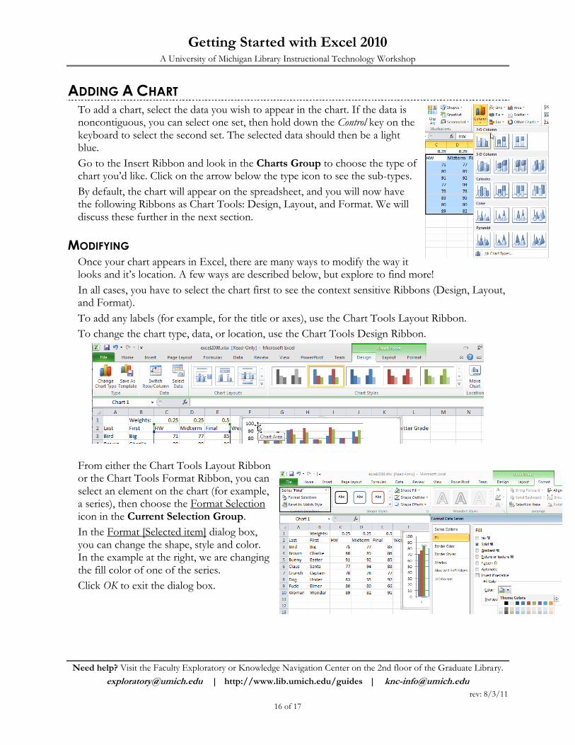
ADDING A CHART To add a chart, select the data you wish to appear in the chart. If the data is noncontiguous, you can select one set, then hold down the Control key on the keyboard to select the second set. The selected data should then be a light blue.

Go to the Insert Ribbon and look in the Charts Group to choose the type of chart you‟d like. Click on the arrow below the type icon to see the sub-types.

By default, the chart will appear on the spreadsheet, and you will now have the following Ribbons as Chart Tools: Design, Layout, and Format. We will discuss these further in the next section.

MODIFYING Once your chart appears in Excel, there are many ways to modify the way it looks and it‟s location. A few ways are described below, but explore to find more!

In all cases, you have to select the chart first to see the context sensitive Ribbons (Design, Layout, and Format).

To add any labels (for example, for the title or axes), use the Chart Tools Layout Ribbon.

To change the chart type, data, or location, use the Chart Tools Design Ribbon.

From either the Chart Tools Layout Ribbon or the Chart Tools Format Ribbon, you can select an element on the chart (for example, a series), then choose the Format Selection icon in the Current Selection Group.

In the Format [Selected item] dialog box, you can change the shape, style and color. In the example at the right, we are changing the fill color of one of the series.

Click OK to exit the dialog box.




rev: 8/3/11

17 of 17

WORKING WITH PIVOT TABLES A pivot table is a way to summarize and view large amounts of raw data in an easy to read format. The pivot table doesn‟t change your raw data, but rather creates a new view of it. While there are many more things you can do with pivot tables than the below, let‟s look at an example.

SELECTING THE DATA 1. Put your cursor anywhere in your

data set (you don‟t have to select it all), then go to the Insert Ribbon and click on the Pivot table icon to the far left.

2. Excel will guess at which data should be included; if it‟s wrong, select the correct data in the Table/Range: field of the Create PivotTable dialog box.

3. It‟s most common to put the pivot table in a new sheet, but you could change the radio button in the Choose where you want the PivotTable report to be placed section of the dialog box. Click OK.

CREATING THE REPORT When you click OK, you will be brought to a new sheet that lists your column headings to the right side of the screen and a box that suggests how to build the pivot table.

1. To create the pivot table, choose fields from the upper right that will display in the report.

2. Click on the pulldown arrow next to the item in the Values area to change the function.

3. Click on the arrow next to the Row Labels to filter and sort.

4. If you change your data on the source spreadsheet, be sure to click on the Refresh icon in the PivotTable Tools Options Ribbon.

a university of michigan library instructional technology ... · getting started with excel 2010 a...

Documents