a uni–ed approach to systemic risk measures via acceptance...

A unied approach to systemic risk measures viaacceptance set

Marco Frittelli(Joint paper with Francesca Biagini, Jean-Pierre Fouque, Thilo

Meyer-Brandis)

Workshop I: Systemic Risk and Financial NetworksPart of the Long Program: Broad Perspectives and New Directions in

Financial MathematicsMarch 24, 2015, IPAM, Los Angeles

Marco Frittelli, University of Milano () Systemic Risk Measures IPAM 2015 1 / 62

Outline

The classical set up:

Coherent and Convex risk measuresDegree of acceptability (Quasi-Convexity)General Capital Requirements

Systemic Risk Measures (SRM)

Aggregation functionsFirst aggregate, second add capital


Outline

In our approach

We contemplate both

rst aggregate and second add capitalrst add capital and second aggregate

We not only allow adding cash but we permit adding random capitalWe employ multidimensional acceptance setsWe allow for degrees of acceptability

Denitions and properties

Some classes of SRM in our approach

Applications

Random cash allocationGaussian nancial systemModel of borrowing and lendingFinite probability space model


Monetary Risk Measures

A monetary risk measure is a map

η : L0(R)! R

that can be interpreted as the minimal capital needed to secure anancial position with payo¤ X 2 L0(R), i.e. the minimal amountm 2 R that must be added to X in order to make the resulting payo¤ attime T acceptable:

η(X ) , inffm 2 R j X +m 2 Ag,

where the acceptance setA L0(R)

is assumed to be monotone, i.e.

X Y 2 A implies X 2 A.


Coherent / Convex Risk MeasuresArtzner, Delbaen, Eber and Heath (1999); Föllmer and Schied (2002); F. and RosazzaGianin (2002)

In addition to decreasing monotonicity, the characterizing feature of thesemonetary maps is the cash additivity property:

η(X +m) = η(X )m, for all m 2 R.

Under the assumption that the set A is convex (resp. is a convex cone)the maps

η(X ) := inffm 2 R j X +m 2 Ag,are convex (resp. convex and positively homogeneous) and are calledconvex (resp. coherent) risk measures.


Diversication

The principle that diversication should not increase the risk ismathematically translated not necessarily with the convexity property butwith the weaker condition of quasiconvexity:

η(λX + (1 λ)Y ) η(X ) _ η(Y ).

As a result in Cerreia-Vioglio, Maccheroni, Marinacci Montrucchio 2010,the only properties assumed in the denition of a quasi-convex riskmeasure are decreasing monotonicity and quasiconvexity.


Quasi-convex Risk MeasuresDegree of acceptability: Cherny Madan 2009

Such quasi-convex risk measures can always be written as:

η(X ) , inffm 2 R j X 2 Amg, (1)

where each set Am L0(R) is monotone and convex, for each m 2 R.

Am is the class of payo¤s carrying the same risk level m 2 R.

Contrary to the convex cash additive case, where each random variable isbinary cataloged as acceptable or as not acceptable, in the quasi-convexcase one admits various degrees of acceptability, described by therisk level m

By selecting Am := Am, the convex cash additive risk measure isclearly a particular case of the one in (1).


General Capital RequirementF. and Scandolo 2006

η(X ) , inffm 2 R j X +m1 2 Ag, A L0(R)Why should we consider only moneyas safe capital ?

One should be more liberal and permit the use of other nancial assets(other than the bond := 1), in an appropriate set C of safe instruments,to hedge the position X .

DenitionThe general capital requirement is

η(X ) , inffπ(Y ) 2 R j Y 2 C, X + Y 2 Ag,

for some evaluation functional π : C ! R.

This is exactly the approach taken by F-Scandolo 2006.


Systemic Risk Measure

Consider a system of N interacting nancial institutions and a vectorX = (X 1, . . . ,XN ) 2 L0(RN ) := L0(Ω,F ;RN ) of associated risk factors(nancial positions) at a given future time horizon T .

In this paper we are interested in real-valued systemic risk measures:

ρ : L0(RN)! R

that evaluates the risk ρ(X) of the complete nancial system X.

Many of the SRM in the existing literature are of the form

ρ(X) = η(Λ(X)),

where η : L0(R)! R is a univariate risk measure and

Λ : RN ! R

is an aggregation rule that aggregates the N-dimensional risk factor Xinto a univariate risk factor Λ(X) representing the total risk in thesystem.


Systemic Risk Measure

Consider a system of N interacting nancial institutions and a vectorX = (X 1, . . . ,XN ) 2 L0(RN ) := L0(Ω,F ;RN ) of associated risk factors(nancial positions) at a given future time horizon T .

In this paper we are interested in real-valued systemic risk measures:

ρ : L0(RN)! R

that evaluates the risk ρ(X) of the complete nancial system X.Many of the SRM in the existing literature are of the form

ρ(X) = η(Λ(X)),

where η : L0(R)! R is a univariate risk measure and

Λ : RN ! R

is an aggregation rule that aggregates the N-dimensional risk factor Xinto a univariate risk factor Λ(X) representing the total risk in thesystem.


Examples of aggregation rule

Λ(x) = ∑Ni=1 xi , x = (x1, ..., xN ) 2 RN .

Λ(x) =N

∑i=1xi or Λ(x) =

N

∑i=1(xi di ), di 2 R

takes into account the lack of cross-subsidization between nancialinstitutions

Eisenberg and Noe: accounts for counterparty contagion.

Λ(x) =N

∑i=1 exp (αixi ), αi 2 R+

Λ(x) =N



First aggregate, second add capitalcash additive case

ρ(X) = η(Λ(X)),

If η is a convex (cash additive) risk measure then we can rewrite such ρ as

ρ(X) , inffm 2 R j Λ(X) +m 2 Ag . (2)

The SRM is the minimal capital needed to secure the system afteraggregating individual risks

If Λ(X) is not capital, the risk measure in (2) is some general risk level ofthe system.

For an axiomatic approach for this type of SRM see Chen IyengarMoallemi 2013 and Kromer Overbeck Zilch 2013 and the referencestherein. Acharya et al. 2010, Adrian Brunnermeier 2011, CheriditoBrunnermeier 2014, Gauthier Lehar Souissi 2010, Ho¤mannMeyer-Brandis Svindland 2014, Huang Zhou Zhu 2009, Lehar 2005.


First aggregate, second add capitalcash additive case

ρ(X) = η(Λ(X)),

If η is a convex (cash additive) risk measure then we can rewrite such ρ as

ρ(X) , inffm 2 R j Λ(X) +m 2 Ag . (2)

The SRM is the minimal capital needed to secure the system afteraggregating individual risksIf Λ(X) is not capital, the risk measure in (2) is some general risk level ofthe system.

For an axiomatic approach for this type of SRM see Chen IyengarMoallemi 2013 and Kromer Overbeck Zilch 2013 and the referencestherein. Acharya et al. 2010, Adrian Brunnermeier 2011, CheriditoBrunnermeier 2014, Gauthier Lehar Souissi 2010, Ho¤mannMeyer-Brandis Svindland 2014, Huang Zhou Zhu 2009, Lehar 2005.


First aggregate, second add capitalThe quasi-convex case

Similarly, if η is a quasi-convex risk measure the systemic risk measure then

ρ(X) = η(Λ(X))

can be rewritten as

ρ(X) , inffm 2 R j Λ(X) 2 Amg.

Again one rst aggregates the risk factors via the function Λ and in asecond step one computes the minimal risk level associated to the totalsystem risk Λ(X).


Purpose of this paper

The purpose of this paper is to specify a general methodologicalframework that is exible enough to cover a wide range of possibilitiesto design systemic risk measures via acceptance sets and aggregationfunctions and to study corresponding examples.

We extend the conceptual framework for systemic risk measures viaacceptance sets step by step in order to gradually include certainnovel key features of our approach.


Key feature 1: First add capital, second aggregate

A regulator might have the possibility to intervene on the level of thesingle institutions before contagion e¤ects generate further losses.

Then it might be more relevant to measure systemic risk as theminimal capital that secures the aggregated system by injectingthe capital into the single institutions before aggregating theindividual risks.


First add capital, second aggregate

ρ(X) , inffN

∑i=1mi 2 R j m = (m1, ...,mN ) 2 RN ; Λ(X+m) 2 Ag .

The amount mi is added to the nancial position X i before thecorresponding total loss Λ(X+m) is computed.The systemic risk is the minimal total capital ∑N

i=1mi injected intothe institutions to secure the system.

ρ delivers at the same time a measure of total systemic risk and apotential ranking of the institutions in terms of systemic riskiness.

Suppose ρ(X) = ∑Ni=1m

i .

Then one could argue that the risk factor Xi1 that requires the biggestcapital allocation mi1 corresponds to the riskiest institution, and so on.When the allocation m is not unique, one has to discuss criteria thatjustify the choice of a specic allocation.


First add capital, second aggregate

ρ(X) , inffN

∑i=1mi 2 R j m = (m1, ...,mN ) 2 RN ; Λ(X+m) 2 Ag .

The amount mi is added to the nancial position X i before thecorresponding total loss Λ(X+m) is computed.The systemic risk is the minimal total capital ∑N

i=1mi injected intothe institutions to secure the system.

ρ delivers at the same time a measure of total systemic risk and apotential ranking of the institutions in terms of systemic riskiness.

Suppose ρ(X) = ∑Ni=1m

i .

Then one could argue that the risk factor Xi1 that requires the biggestcapital allocation mi1 corresponds to the riskiest institution, and so on.When the allocation m is not unique, one has to discuss criteria thatjustify the choice of a specic allocation.Marco Frittelli, University of Milano () Systemic Risk Measures IPAM 2015 15 / 62

Key feature 2: Random allocation

We allow for the possibility of adding to X not merely a vectorm = (m1, ...,mN ) 2 RN of cash but a random vector

Y 2 C L0(RN )

which represents, in the spirit of F. and Scandolo, admissible nancialassets that can be used to secure a system by adding Y to Xcomponent-wise.To each Y 2 C we assign a measure π(Y) of the cost associated to Ydetermined by a monotone increasing map

π : C ! R

Hence:ρ(X) , inffπ(Y) 2 R j Y 2 C; Λ(X+Y) 2 Ag .

If ρ(X) = π(Y) and Y = (Y 1 , ...,YN ) 2 C is optimal, an ordering

of the Y 1 , ...,YN may induce a systemic ranking of the institution

(X1, ...,XN ).


Key feature 2: Random allocation

We allow for the possibility of adding to X not merely a vectorm = (m1, ...,mN ) 2 RN of cash but a random vector

Y 2 C L0(RN )

which represents, in the spirit of F. and Scandolo, admissible nancialassets that can be used to secure a system by adding Y to Xcomponent-wise.To each Y 2 C we assign a measure π(Y) of the cost associated to Ydetermined by a monotone increasing map

π : C ! R

Hence:ρ(X) , inffπ(Y) 2 R j Y 2 C; Λ(X+Y) 2 Ag .

If ρ(X) = π(Y) and Y = (Y 1 , ...,YN ) 2 C is optimal, an ordering

of the Y 1 , ...,YN may induce a systemic ranking of the institution

(X1, ...,XN ).Marco Frittelli, University of Milano () Systemic Risk Measures IPAM 2015 16 / 62

Particular case: lender of last resort

C fY 2 L0(RN ) jN

∑n=1

Y n 2 Rg =: CR,

and set π(Y) = ∑Nn=1 Y

n.

ρ(X) , inffN

∑n=1

Y n j Y 2 C; Λ(X+Y) 2 Ag

is the minimal total cash amount ∑Nn=1 Y

n 2 R needed today to securethe system by distributing the capital at time T among (X 1, ...,XN ).

In general the allocation Y i (ω) to institution i does not need to bedecided today but depends on the scenario ω realized at time T .For C = RN the situation corresponds to the previous case where thedistribution is already determined today.For C = CR the distribution can be chosen freely depending on thescenario ω realized in T (including negative amounts, i.e.withdrawals of cash from certain components).



C fY 2 L0(RN ) jN

∑n=1

Y n 2 Rg =: CR,


n.

ρ(X) , inffN

∑n=1




In general the allocation Y i (ω) to institution i does not need to bedecided today but depends on the scenario ω realized at time T .

For C = RN the situation corresponds to the previous case where thedistribution is already determined today.For C = CR the distribution can be chosen freely depending on thescenario ω realized in T (including negative amounts, i.e.withdrawals of cash from certain components).



C fY 2 L0(RN ) jN

∑n=1

Y n 2 Rg =: CR,


n.

ρ(X) , inffN

∑n=1




In general the allocation Y i (ω) to institution i does not need to bedecided today but depends on the scenario ω realized at time T .For C = RN the situation corresponds to the previous case where thedistribution is already determined today.For C = CR the distribution can be chosen freely depending on thescenario ω realized in T (including negative amounts, i.e.withdrawals of cash from certain components).


Dependence can be taken into account

Allowing random allocations of cash Y 2 C CR the systemic riskmeasure will take the dependence structure of the components of X intoaccount even though acceptable positions might be dened in terms of themarginal distributions of Xi , i = 1, ...,N, only.


Example: dependence may be taken into account

Λ(x) := ∑Ni=1 xi , x 2 RN ,

A := fZ 2 L0(R) j E [Z ] γg ,γ 2 R.Z 2 L0(RN ) is acceptable if and only if Λ(Z) 2 A, i.e.

N

∑i=1E [Zi ] γ ,

which only depends on the marginal distributions of Z.

If C = RN then ρ(X) will depends on the marginal distributions of Xonly.

If one allows for more general allocations of cash Y 2 C CR thatmight di¤er from scenario to scenario the systemic risk measure will ingeneral depend on the multivariate distribution of X since it can playon the dependence of the components of X to minimize the costs.


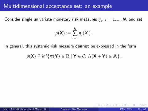
Multidimensional acceptance set: an example

Consider single univariate monetary risk measures ηi , i = 1, ...,N, and set

ρ(X) :=N

∑i=1

ηi (Xi ) .

In general, this systemic risk measure cannot be expressed in the form

ρ(X) , inffπ(Y) 2 R j Y 2 C; Λ(X+Y) 2 Ag .

If Ai L0(R) is the acceptance set of ηi , i = 1, ...,N, then it is possibleto write such ρ = ∑N

i=1 ηi (Xi ) in terms of the multivariate acceptance setA1 ...AN :

ρ(X) , inffN

∑i=1mi j m = (m1, ...,mN ) 2 RN ,X+m 2 A1 ...ANg .


Key feature 3: General multidimensional acceptance set

We extend our formulation of systemic risk measures as the minimal costof admissible asset vectors Y 2 C that, when added to the vector ofnancial positions X, makes the augmented nancial positions X+Yacceptable in terms of a general multidimensional acceptance set

A L0(RN )

ρ(X) , inffπ(Y) 2 R j Y 2 C; X+Y 2 Ag . (3)

Our previous denition of systemic risk measure

ρ(X) , inffπ(Y) 2 R j Y 2 C; Λ(X+Y) 2 Ag .

is therefore a particular case of (3): just let

A :=nZ 2 L0(RN ) j Λ(Z) 2 A

oMarco Frittelli, University of Milano () Systemic Risk Measures IPAM 2015 21 / 62

Generalized cash invariance

The systemic risk measure

ρ(X) , inffπ(Y) 2 R j Y 2 C; X+Y 2 Ag

exhibit an extended type of cash invariance:

ρ(X+Y) = ρ(X) + π(Y)

for Y 2 C such that Y0 Y 2 C for all Y0 2 C.


General form of Systemic Risk MeasureKey feature 4: Degree of acceptability

Recall the one dimensional case:

η(X ) , inffm 2 R j X 2 Amg

Our general systemic risk measure is dened by:

ρ(X) , inffπ(Y) 2 R j Y 2 C, X 2 AYg . (4)

We associate to each Y 2 C a set AY L0(RN ) of risk vectors that areacceptable for the given (random) vector Y.Then ρ(X) represents some minimal aggregated risk level π(Y) at whichthe system X is acceptable.

The approach in (4) is very exible and it includes all previous cases ifwe set

AY := AY,where the set A L0(RN ) represents acceptable risk vectors.


General form of Systemic Risk MeasureKey feature 4: Degree of acceptability

Recall the one dimensional case:

η(X ) , inffm 2 R j X 2 Amg

Our general systemic risk measure is dened by:

ρ(X) , inffπ(Y) 2 R j Y 2 C, X 2 AYg . (4)

We associate to each Y 2 C a set AY L0(RN ) of risk vectors that areacceptable for the given (random) vector Y.Then ρ(X) represents some minimal aggregated risk level π(Y) at whichthe system X is acceptable.The approach in (4) is very exible and it includes all previous cases ifwe set

AY := AY,where the set A L0(RN ) represents acceptable risk vectors.Marco Frittelli, University of Milano () Systemic Risk Measures IPAM 2015 23 / 62

General aggregation functional

Another advantage of the formulation in terms of general acceptance setsAY is the possibility to design systemic risk measures via generalaggregation rules. Indeed our last formulation includes the case

ρ(X) , inffπ(Y) 2 R j Y 2 C, Θ(X,Y) 2 Agwhere Θ : L0(RN ) C ! L0(R) denotes some aggregation functionjointly in X and Y. Just select

AY :=nZ 2 L0(RN ) j Θ(Z,Y) 2 A

oThis formulation includes

aggregation before injecting capital by puttingΘ(X,Y) :=Λ1(X)+Λ2(Y), where Λ1 : L0(RN )! L0(R) is anaggregation function and Λ2 : C ! L0(R) could be, for example,Λ2 = π.injecting capital before aggregation by puttingΘ(X,Y) =Λ(X+Y),


Summarizing our approach

ρ(X) , inffπ(Y) 2 R j Y 2 C, X 2 AYg .

We contemplate both

rst aggregate and second add capitalrst add capital and second aggregate

We not only allow adding cash but we permit adding random capital

We employ multidimensional acceptance sets

We allow for degrees of acceptability


Structure of the paper

1 We provide su¢ cient condition on π, C , AY so that the SystemicRisk Measure (SRM)

ρ(X) , inffπ(Y) 2 R j Y 2 C, X 2 AYg

is a well dened monotone decreasing and quasi-convex (orconvex) map ρ : L0(RN )! R.

2 We provide four classes of Systemic Risk Measures, satisfying theconditions in item (1) above, dened via one dimensional acceptancesets and aggregation functions Λ : L0(RN ) C ! L0(R).

3 We study the particular case of random cash allocations, i.e. when:

C fY 2 L0(RN ) jN

∑n=1

Y n 2 Rg =: CR.



4 For a Gaussian nancial system, i.e. if X N(µ,Q), we study theSRM

ρ(X) : = inf

(N

∑i=1Yi j Y 2 C CR , Λ(X+Y) 2 Aγ

),

Λ(X) : =N

∑i=1(Xi di ), di 2 R,

Aγ : =Z 2 L0(R)jE [Z ] γ

, γ 2 R+.

in the two cases: C := RN, and

C :=

(Y 2 L0(Rn)jY = m+ αID , m, α 2 RN ,

N

∑i=1

αi = 0

) CR,

where D := f∑ni=1 Xi dg , for some d 2 R



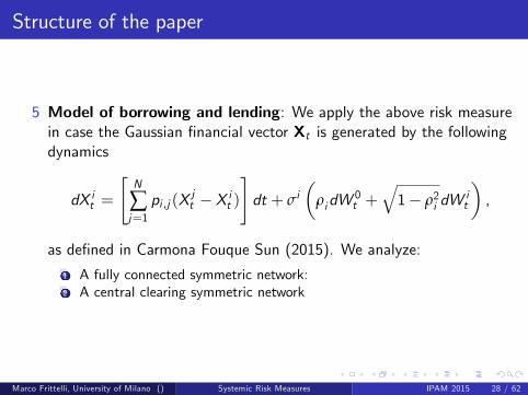
5 Model of borrowing and lending: We apply the above risk measurein case the Gaussian nancial vector Xt is generated by the followingdynamics

dX it =

"N

∑j=1pi ,j (X

jt X it )

#dt + σi

ρidW

0t +

q1 ρ2i dW

it

,

as dened in Carmona Fouque Sun (2015). We analyze:

1 A fully connected symmetric network:2 A central clearing symmetric network



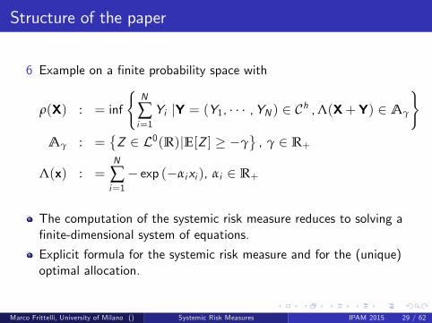
6 Example on a nite probability space with

ρ(X) : = inf

(N

∑i=1Yi jY = (Y1, ,YN ) 2 Ch ,Λ(X+Y) 2 Aγ

)Aγ : =

Z 2 L0(R)jE[Z ] γ

, γ 2 R+

Λ(x) : =N


The computation of the systemic risk measure reduces to solving anite-dimensional system of equations.

Explicit formula for the systemic risk measure and for the (unique)optimal allocation.


1: Setting

Denition

The systemic risk measure associated with C,AY and π is a mapρ : L0(RN )! R, dened by:

ρ(X) := inffπ(Y) 2 R j Y 2 C, X 2 AYg ,

Moreover ρ is called a quasi-convex (resp. convex) systemic risk measure ifit is -monotone decreasing and quasi-convex (resp. convex onfρ(X) < +∞g).


1: Su¢ cient conditions

1 For all Y 2 C the set AY L0(RN ) is -monotone.2 For all m 2 R, for all Y1,Y2 2 C such that π(Y1) m and

π(Y2) m and for all X1 2 AY1 , X2 2 AY2 and all λ 2 [0, 1] thereexists Y 2 C such that π(Y) m and λX1 + (1 λ)X2 2 AY.

3 For all Y1,Y2 2 C and all X1 2 AY1 , X2 2 AY2 and all λ 2 [0, 1]there exists Y 2 C such that π(Y) λπ(Y1) + (1 λ)π(Y2) andλX1 + (1 λ)X2 2 AY.

Fact.

a If the systemic risk measure ρ satises the properties 1 and 2, then ρis -monotone decreasing and quasi-convex.

b If the systemic risk measure ρ satises the properties 1 and 3, then ρis -monotone decreasing and convex on fρ(X) < +∞g.


1: Alternative su¢ cient conditions

1 For all Y 2 C the set AY L0(RN ) is -monotone.2a For all Y1,Y2 2 C, X1 2 AY1 , X2 2 AY2 and λ 2 [0, 1] there exists

α 2 [0, 1] such that λX1 + (1 λ)X2 2 AαY1+(1α)Y2

3a For all Y1,Y2 2 C, X1 2 AY1 , X2 2 AY2 and λ 2 [0, 1] it holds:λX1 + (1 λ)X2 2 AλY1+(1λ)Y2 .

4 C is convex,5 π is quasi-convex,

6 π is convex.

Fact.

a Under the conditions 1, 2a, 4, and 5 the map ρ is a quasi-convexSRM.

b Under the conditions 1, 3a, 4 and 6, the map ρ is a convex SRM.


2: SRM via general aggregation functions and acceptanceset

The following three assumptions hold true in the next propositions.

1 The aggregation functions are dened by:

Λ : L0(RN ) C ! L0(R),Λ1 : L0(RN )! L0(R),

2 The acceptance family(Am)m2R,

of monotone convex subsets Am L0(R), is supposed an increasingfamily w.r.to m 2 R

3 The monotone and convex acceptance subset is:

A L0(R).


2: Family of SRM

Proposition

If C is convex, if π is quasi-convex, Λ is concave and Λ(,Y) is-increasing for all Y 2C then the map

ρ(X) , inffπ(Y) 2 R j Y 2 C, Λ(X,Y) 2 Ag

is a quasi-convex SRM; if in addition π is convex then ρ is a convex SRM.

Notice that such a risk measure may describe both cases:

rst aggregate and second add the capital : for example ifΛ(X,Y) :=Λ1(X)+Λ2(Y), where Λ2(Y) could be interpreted as thediscounted cost of Y)rst add and second aggregate: for example if Λ(X,Y) :=Λ1(X+Y).


2: Family of SRM

PropositionIf C is convex, if π is quasi-convex, if Λ1 is -increasing and concave, ifθ : C ! R then

ρ(X) := inffπ(Y) 2 R j Y 2 C, Λ1(X) 2 Aθ(Y)g

is a (truly) quasi-convex SRM.

This SRM represents the generalization of the quasi-convex classicalone dimensional risk measure

η(X ) , inffm 2 R j X 2 Amg,

.


2: Family of SRM

PropositionSuppose:

1 0 2C L0(RN ) is a convex set, C +RN+ 2 C

2 π satises π(u) = 1, for a xed u 2 RN+ and

π(α1Y1 + α2Y2) = α1π(Y1) + α2π(Y2)

for all αi 2 R+ and Yi 2 C3 Λ is concave and Λ(X, ) : C ! L0(R) is increasing for allX 2L0(RN ).

Then the map

ρ(X) = inffπ(Y) 2 R j Y 2 C, Λ(X,Y) 2 Aπ(Y)g

is a quasi-convex SRM.


3: Random cash allocations

We study the particular case of random cash allocations, i.e. when:

C fY 2 L0(RN ) jN

∑n=1

Y n 2 Rg =: CR.


3: Random cash allocations

C fY 2 L0(RN ) jN

∑n=1

Y n 2 Rg =: CR and C +RN+ 2 C.

ρ(X) := inffN

∑n=1

Y n j Y 2 C, X+Y 2 Aθ(∑Y n)g ,

If θ : R ! R is increasing then ρ is a (truly) quasi-convex SRM.

The criteria whether a system is safe or not after injecting a capitalvector Y is given by the (N-dimensional) acceptance set Aθ(∑Y n)

which itself depends on the total cash amount ∑Nn=1 Y

n.

Model an increasing level of prudence when dening safe systemsfor higher amounts of required total capital.


3: A particular case

In the case C = CR then every systemic risk measure of this type can bewritten as a univariate quasi-convex risk measure applied to the sum of therisk factors:If C = CR then

ρ(X) := inffN

∑n=1

Y n j Y 2 C, X+Y 2 Aθ(∑Y n)g ,

is of the form

ρ(X) = eρ( N∑n=1

X n)

for some quasi-convex risk measure

eρ : L0(R)! R.


3: Example: Worst case type of risk measuresWe compare: injecting capital before or after aggregation

Fix A := L0+(R),

Λ(X) : =N

∑i=1(Xi ),

π(Y) : =n

∑i=1Yi

Deterministic or random allocations:

C = RN

Cγ : = fY 2 CR j Yi γi g , γi 2 [∞, 0], i = 1, ...N

(for γ := (∞, ...,∞) this family of subsets includes C∞ = CR).


3: Continuing the exampleWe compare: injecting capital before or after aggregation

We compare: rst aggregate and second injecting capital:

ρag (X) := inf fy 2 R j Λ(X) + y 2 Ag = ρWorst (N

∑i=1(Xi )) ,

and rst injecting capital and second aggregatefor both the deterministic cash allocations:

ρRN(X) := inf

nπ(Y) j Y 2 RN ,Λ(X+Y) 2 A

o,

and the random cash allocations:

ργ(X) := inf fπ(Y) j Y 2 Cγ ,Λ(X+Y) 2 Ag .


3: Continuing the example

ρag (X) rst aggregate second add capitalρRN

(X) rst add second aggregate: deterministic cashργ(X) rst add second aggregate: random cash

Then one obtains:

ρRN(X) =

N

∑i=1

ρWorst (Xi ) ρag (X)

ργ(X) = ρWorst

N

∑i=1(XiIXiγi γiIXiγi )

! ρag (X) ,

If γ = 0 := (0, ..., 0) then ρ0(X) = ρag (X),If γ = ∞ := (∞, ...,∞) then ρ∞(X) = ρWorst (∑

Ni=1 Xi ).

The interplay between A and Λ is critical.


3: Example: Expected ShortfallSame example but with di¤erent acceptance set

AES := fX 2 L0(R) j ρES (X ) 0gEverything else is as in the previous Example. Then

ρag (X) = ρES (N

∑i=1(Xi )).

For ρRNand ργ, however, AES gives the same result as AWorst , i.e.

ρRN(X) =

N

∑i=1

ρWorst (Xi ) ρag (X)

ργ(X) = ρWorst (N

∑i=1(XiIXiγi γiIXiγi )) .


4: Gaussian nancial system

We now illustrate the application to the Gaussian nancial system


4: Gaussian nancial system

Consider a Gaussian nancial system, i.e. X = (X1, ,XN ) is anN-dimensional vector with X N(µ,Q), [Q ]ii := σ2i , and [Q ]ij := ρi ,j fori 6= j , and mean vector µ := (µ1, , µN ).

ρ(X) : = inf

(N

∑i=1Yi j Y 2 C CR , Λ(X+Y) 2 Aγ

),

Λ(X) : =N

∑i=1(Xi di ), di 2 R,

Aγ : =Z 2 L0(R)jE [Z ] γ

, γ 2 R+.

di in the aggregation rule denotes some critical liquidity level of institutioni and the risk measure is concerned with the expected total shortfall belowthese levels in the system

First, we consider the case: C := RN

Second, we consider a random allocationThird we compare the above two cases.


Example: Gaussian case with deterministic allocation

Let C = RN and

ρ(X) := inf

(N

∑i=1mi j m = (m1, ,mN ) 2 RN , Λ(X+m) 2 Aγ

),

By solving the Lagrangian system we obtain that the global minimumpoint m = (m1 , ,mN ) is given by

mi = di µi σiR,

where and R solves the equation (for Φ(x) :=R x+∞

1p2πet

2/2dt):

RΦ(R) +1p2π

expR

2

2

=

γ

∑Ni=1 σi

.

The unique optimal cash allocation m induces a ranking of theinstitutions according to systemic riskiness.

1 ∂mi∂µi= 1: the systemic riskiness decreases with increasing mean.

2 ∂mi∂σi> 0: the systemic riskiness increases with increasing volatility.


4: Example: the Gaussian system with random allocation

We allow for di¤erent allocations of the total capital depending ω.Set D := f∑n

i=1 Xi dg , d 2 R, and

C :=

(Y 2 L0(Rn) j Y = m+ αID , m, α 2 RN ,

N

∑i=1

αi = 0

) CR,

The condition ∑ni=1 αi = 0 implies that ∑n

i=1 Yi is constant a.s.

Flexibility: we let the allocation depend on whether the systemat time T is in trouble or not, represented by the events that∑ni=1 Xi is less or greater than some critical level d , respectively.

The SRM is then:

ρ(X) := inf

(N

∑i=1mi j m+ αID 2 C , Λ(X+m+ αID ) 2 Aγ

).


4: Solving by Lagrange method

We minimize the objective function ∑Ni=1mi over (m, α) 2 R2N under the

constrainsN

∑i=1

αi = 0 andN

∑i=1E [(Xi +mi + αi IA di )] = γ .

We apply the method of Lagrange multipliers to minimize the function

φ(m1, ,mN , α1, , αN1,λ) =N

∑i=1mi + λ (Ψ(m1, ,mN , α1, , αN1) γ) ,

where

Ψ(m1, ,mN , α1, , αN1) :=N1∑i=1

E [(Xi +mi + αi ID di )] + E [(XN +mN N1∑j=1

αj ID dN )].

Obtaining explicit formulas for the derivatives.Marco Frittelli, University of Milano () Systemic Risk Measures IPAM 2015 48 / 62

4: Numerical illustration with two banks (X1,X2)Sensitivity with respect to correlation

ρ(X) = inf fm1 +m2 j m+ αID 2 C , Λ(X+m+ αID ) 2 AγgAγ =

Z 2 L0(R) j E [Z ] γ

D := fX1 + X2 dg

Means of (X1,X2): µ1 = µ2 = 0Standard deviations of (X1,X2): σ1 = 1, σ2 = 3,The acceptance level γ = 0.7The critical level d = 2.

We compare the sensitivities with respect to the correlation ρ1,2 for

deterministic allocation (α = 0)random allocation

For highly positively correlated banks the random allocation does notchange the total capital requirement (m1+m2).However, when they are negatively correlated, one benets from randomallocation since the total allocation (m1+m2) is lower.


4: Numerical illustration with two banks (X1,X2)Sensitivity with respect to correlation

ρ(X) = inf fm1 +m2 j m+ αID 2 C , Λ(X+m+ αID ) 2 AγgAγ =

Z 2 L0(R) j E [Z ] γ

D := fX1 + X2 dg

Means of (X1,X2): µ1 = µ2 = 0Standard deviations of (X1,X2): σ1 = 1, σ2 = 3,The acceptance level γ = 0.7The critical level d = 2.We compare the sensitivities with respect to the correlation ρ1,2 for


For highly positively correlated banks the random allocation does notchange the total capital requirement (m1+m2).However, when they are negatively correlated, one benets from randomallocation since the total allocation (m1+m2) is lower.Marco Frittelli, University of Milano () Systemic Risk Measures IPAM 2015 49 / 62

ρ1,2 # Deterministic Randomm1 0.5766 0.1151

-0.9 m2 1.7333 1.6614ρ = m1 +m2 2.3099 1.7765

m1 0.5766 0.2908-0.5 m2 1.7333 1.7776

ρ = m1 +m2 2.3099 2.0683m1 0.5766 0.4490

0 m2 1.7333 1.7796ρ = m1 +m2 2.3099 2.2286

m1 0.5766 0.54630.5 m2 1.7333 1.7461

ρ = m1 +m2 2.3099 2.2924m1 0.5766 0.5780

0.9 m2 1.7333 1.7310ρ = m1 +m2 2.3099 2.3090

Table: Sensitivity with respect to correlation.


4: Numerical illustration with two banks (X1,X2)Sensitivity with respect to standard deviation

ρ(X) : = inf fm1 +m2 j m+ αID 2 C , Λ(X+m+ αID ) 2 AγgAγ : =

Z 2 L0(R)j E [Z ] γ

D := fX1 + X2 dg

Means of (X1,X2): µ1 = µ2 = 0Standard deviation of X1 is σ1 = 1; Correlation ρ1,2 = 0.5The acceptance level γ = 0.7 ; The critical level d = 2.

We compare the sensitivities with respect to σ2 for


For equal marginals (σ1 = σ2 = 1) random allocation does not change thetotal capital requirement.As σ2 increases, the systemic risk measure increases and the allocationincreases, in agreement with the deterministic case.Random allocation allows for smaller total capital (m1+m2).


4: Numerical illustration with two banks (X1,X2)Sensitivity with respect to standard deviation

ρ(X) : = inf fm1 +m2 j m+ αID 2 C , Λ(X+m+ αID ) 2 AγgAγ : =

Z 2 L0(R)j E [Z ] γ

D := fX1 + X2 dg

Means of (X1,X2): µ1 = µ2 = 0Standard deviation of X1 is σ1 = 1; Correlation ρ1,2 = 0.5The acceptance level γ = 0.7 ; The critical level d = 2.We compare the sensitivities with respect to σ2 for


For equal marginals (σ1 = σ2 = 1) random allocation does not change thetotal capital requirement.As σ2 increases, the systemic risk measure increases and the allocationincreases, in agreement with the deterministic case.Random allocation allows for smaller total capital (m1+m2).Marco Frittelli, University of Milano () Systemic Risk Measures IPAM 2015 51 / 62

σ2 # Deterministic Randomm1 0.1008 0.1008m2 0.1031 0.1031

1 α 0 0.0002ρ = m1 +m2 0.2039 0.2039

m1 0.8168 0.3167m2 4.0816 4.1295

5 α 0 3.5987ρ = m1 +m2 4.8984 4.4462

m1 1.1417 0.4631m2 11.3964 11.4333

10 α 0 6.9909ρ = m1 +m2 12.5381 11.8963

Table: Sensitivity with respect to standard deviation.


5: Borrowing and lending: Carmona Fouque Sun 2015

Let the Gaussian nancial vector Xt be generated by the followingdynamics

dX it =

"N

∑j=1pi ,j (X

jt X it )

#dt + σi

ρidW

0t +

q1 ρ2i dW

it

,

The lending-borrowing preferences pi ,j are nonnegative and symmetric:pi ,j = pj ,i .

W 0t ,W

it , i = 1, ,N

are independent standard BM and

W 0t is a common noise.

The joint distribution of (X 1t , ...,XNt ) will be fully characterized by

the means µis and by the covariance matrix Q which will depend onthe parameters of the model, in particular the preferences pi ,j(lending/borrowing) and the individual σi .Applying the approach just described (in 4), for given parameters,one computes the marginal means and variances needed in oursystemic risk measures, in order to obtain the optimalallocation m = (mi )i=1, ,N and a ranking of the banks.


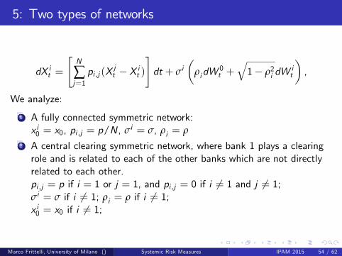
5: Two types of networks

dX it =

"N

∑j=1pi ,j (X

jt X it )

#dt + σi

ρidW

0t +

q1 ρ2i dW

it

,

We analyze:

1 A fully connected symmetric network:x i0 = x0, pi ,j = p/N, σi = σ, ρi = ρ

2 A central clearing symmetric network, where bank 1 plays a clearingrole and is related to each of the other banks which are not directlyrelated to each other.pi ,j = p if i = 1 or j = 1, and pi ,j = 0 if i 6= 1 and j 6= 1;σi = σ if i 6= 1; ρi = ρ if i 6= 1;x i0 = x0 if i 6= 1;


5: Marginals in the fully connected symmetric network

µi = E(X it ) = x0,

σ2i = σ2(1 ρ2)(1 1N)

1 e2pt2p

+ σ2

ρ2 +

1 ρ2

N

t.

These marginal distributions depend on the coupled dynamics of theX i , in particular on the parameters p and ρ.

Increasing p, that is increasing liquidity, would decrease σ2i (from σ2t

for p = 0 to σ2

ρ2 + 1ρ2

N

t for p = ∞), and therefore would

decrease systemic risk.


5: Central clearing symmetric network

µi = E(X it ) = E(X 1t ) = c0/N.

σ21 = σ2ρ2t

+1N

(σ2 + 2σσcρρc 3σ2ρ2)t +

2p(σ2c σσcρρc )

+O( 1

N2),

σ2i = σ2(1 ρ2)

1 e2pt2p

+ σ2ρ2t

+1N

(σ2 + 2σσcρρc 3σ2ρ2)t σ2(1 ρ2)

1 e2pt2p

+O( 1

N2),

At order one in 1/N, this variance is the same as the homogeneous model,but they may di¤er at order 1/N.Writing σ2 + 2σσcρρc 3σ2ρ2 = σ2(1 ρ2) + 2σρ(σcρc σρ), we seethat the sign of σcρc σρ determines which network is most stable(smaller variance).Marco Frittelli, University of Milano () Systemic Risk Measures IPAM 2015 56 / 62

6: Example on a nite probability space

We assume a nite probability space (Ω,F ,P)Ω = fωjg, j = 1, ,MThen the computation of optimal cash allocations associated to thesystemic risk measure reduces to solving a nite-dimensional systemof equations, even for most general random cash allocations, wherethe allocation can be adjusted scenario by scenario.

Explicit formula for the systemic risk measure and for the (unique)optimal allocation.


6: Example on a nite probability space

The Systemic Risk Measure is dened by:

ρ(X) : = inf

(N

∑i=1Yi j Y = (Y1, ,YN ) 2 Ch ,Λ(X+Y) 2 Aγ

)Aγ : =

Z 2 L0(R)jE[Z ] γ

, γ 2 R+

Λ(x) : =N



6: Random allocations in subgroups

The permitted allocations are dened by:

Ch =

Y 2 L0(RN ) j

h1

∑i=1Yi (ωj ) = d1,

h2

∑i=h1+1

Yi (ωj ) = d2, ,

N

∑i=hk1+1

Yi (ωj ) = dk

CR, d1, ..., dk 2 R, 8j .

The regulator is constrained to distribute the capital only withink subgroups that are induced by the partition h = (h1, .., hk ) with0 < h1 < h2 < < hk1 < hk = NThe risk measure is the sum of k minimal cash funds d1, ..., dkdetermined today, that at time T can be freely allocated withinthe k subgroupsNote that this family includes as two extreme cases

deterministic allocations C = RN for k = Ncompletely free allocations C = CR for k = 1.


6: Applying Lagrange method

For a specic subfamily of Ch we obtain the explicit formula for ρ:

ρ(X) = βNr log(γ

α1βNdNr)

N

∑j=Nr+1

1αjlog(

γ

αjβNKj),

where:

βNr =Nr∑i=1

1αi

βN =N

∑i=1

1αi

dNr =M

∑j=1pj exp

" 1

βNr

Nr∑i=1

Xi (wj )1

βNr

Nr∑i=1

1αilog(

α1αi)

#.


6: Applying Lagrange method

and the optimal allocations are given by:

y j1 =1

α1βNr

Nr∑i=1

Xi (wj )X1(wj )+1

α1βNr

Nr∑i=1

1αilog(

α1αi)+

1α1βNr

cNr

for j = 1, ,M; by

y jk =1

αk

α1X1(wj ) αkXk (wj ) log(

α1αk) + α1y

j1

=

1αk βNr

Nr∑i=1

Xi (wj ) Xk (wj )1

αklog(

α1αk)

+1

αk βNr

Nr∑i=1

1αilog(

α1αi) +

1αk βNr

cNr

for all k = 2, ,N r 1 and j 2 1, ,M; and by:

y jk = ck ck1 = 1

αklog(

γ

αk βNKk)

for all k = N r , ,N and j 2 1, ,M.Marco Frittelli, University of Milano () Systemic Risk Measures IPAM 2015 61 / 62

Thank you for your attention


a uni–ed approach to systemic risk measures via acceptance...

Documents