. Report 930-490

A Two-DIMENSIONAL NUMERICAL MODEL STUDY OF CLEAR-WATER

SCOUR AT A BRIDGE CONTRACTION WITH A COHESIVE BED

Prepared by

JACOB P. McLEAN

JOHN E. CURRY

OKTAY GOVEN

JOEL G. MELVILLE

Prepared for

ALABAMA DEPARTMENT OF TRANSPORTATION

MONTGOMERY, ALABAMA

APRIL 2003

A TWO-DIMENSIONAL NUMERICAL MODEL STUDY OF CLEAR-WATER

SCOUR AT A BRIDGE CONTRACTION WITH A COHESIVE BED

Prepared by

Jacob P. McLean Oktay Giiven John E. Curry

Joel G. Melville

Highway Research Center Harbert Engineering Center

Auburn University, Alabama 36849

April 2003

ABSTRACT

Recently, Guven et al. (2001,2002) presented a one-dimensional approach for

modeling time-dependent clear-water contraction scour in a cohesive soil, where the

scour rate for the soil is described by an erosion function. This report extends that

method by using a two-dimensional model to calculate scour. The output from the two-

dimensional Finite Element Surface Water Modeling System (FESWMS) model in the,

Surfacewater Modeling System (SMS) software provides sufficient information to

I

calculate scour over time at desired time steps for the entire two-dimensional domain.

For this study, a 4: 1 bridge contraction with a beveled abutment geometry was

investigated. The model output (velocity, depth, and water surface) and the SMS data

calculator, which allows the user to calculate new data sets from existing ones, are used

to calculate time-dependent scour based on the erosion function at each coordinate in the

model. The erosion function describes the erosion rate for a given soil. For the time-

dependent method, the bed elevation is then updated at each node in the model, and the

streambed is set at a new elevation so that the model can be run again to obtain new

output. While it is possible to change the flow rate for each time step, the flow rate was

kept constant for this study.

An ultimate scour depth (referred to in Guven et al. (2002) as "maximum scour

depth") can also be calculated based on the unit flow rate and other model parameters at a

particular time step.

This report covers the methodology and results for calculating time-dependent as

well as ultimate scour using a two-dimensional [mite element computer model.

ii

ACKNOWLEDGEMENTS

This study was supported by the Alabama Department of Transportation

(Research Project No. 930-490) and administered by the Highway Research Center of

Auburn University. The authors thank Dr. Frazier Parker for his support as Director of

the Highway Research Center. The authors also thank Ms. Priscilla Clark who helped

with the publication of the report.

111

TABLE OF CONTENTS

ABSTRACT ......................................................................................... .ii

ACKNOWLEDGEMENTS ....................................................................... .iii

LIST OF FIGURES .................................................................................. v

1. INTRODUCTION ................................................................................. 1

1.1 Purpose ..... , .............................................................................. 1

" . 1.2 Choice of Base Case .................................................................... 2

1.3 Model Behaviof. ........................................................................ 4

2. SCOUR CALCULATIONS METHODOLOGY ............................................ 13

2.1 Time Dependent Scour Calculation Method ....................................... 13

2.2 Ultimate Scour Calculation Method ............................................... 16

3. RESULTS AND DISCUSSION OF SCOUR CALCULATIONS ...................... .19

3.1 Time Dependent Scour Results ...................................................... 19

3.2 Ultimate Scour Results .............................................................. .29

4. FURTHER INVESTIGATIONS INTO METHODOLOGy .............................. 33

4.1 Effect of Time Step Size ............................................................. 33

4.2 Effect of Second Order Correction ................................................. 33

4.3 Effect of Roughness .................................................................. .37

4.4 Effect of Swamee-Jain Explicit Formula Versus Henderson Implicit Formula to Calculate f. ..................................... ..40

5. CONCLUDING REMARKS .................................................................. 43

REFERENCES ........................................... ; .......................................... 44

IV

LIST OF FIGURES

Figure 1. Base case SMS model geometry and boundary conditions .......................... 3

Figure 2. Velocity, depth, and unit flow rate distribution for the base case .................. 5

Figure 3. Transverse velocity profile for the base case at entrance to contraction (x = -30 ft) .................................................. 7

Figure 4. Transverse bed and water surface profiles for the base case at entrance to contraction (x = -30 ft) ................................................. 8

Figure 5. Transverse unit flow rate (q) profile for the base case at entrance to contraction (x = -30 ft) ................................................. 9

Figure 6. Transverse velocity profile for the base case at midpoint of contraction (x = 0 ft) ................................. , ............... 1 0

Figure 7. Transverse bed and water surface profiles for the base case at midpoint of contraction (x = 0 ft) ................................................. 11

Figure 8. Transverse unit flow rate (q) profile for the base case at midpoint of contraction (x = 0 ft) .................................................. 12

Figure 9. Distribution of bed shear stress (lb/ft2) for the base case at time t = 0 ........... 20

Figure 10. Bed elevation (ft) contours at times t = 10, 50, and 150 days (top to bottom) ............................................................. .21

Figure 11. Longitudinal plot of water surface and bed elevation along centerline from x = -500 to 1500 ft at times 0, 50, and 150 days and for ultimate scour based on conditions for ti = 150 days ..................... 22

Figure 12. Longitudinal plot of unit flow rate (q) along centerline from x = -500 to 1500 ft at times 0, 50, and 150 days and for ultimate scour based on conditions for ti = 150 days ......................... 23

Figure 13. Transverse bed and water surface profiles at midpoint of contraction (x = 0 ft) at times 0,50, and 150 days and for ultimate scour based on conditions for ti = 150 days ..................... 24

v

Figure 14. Transverse unit flow rate (q) profile at midpoint of contraction (x = ° ft) at times 0, 50, and 150 days and for ultimate scour based on conditions for ti = 150 days ........................ .25

Figure 15 .. Transverse bed and water surface profiles at entrance to contraction (x = -30 ft) at times 0, 50, and 150 days aJ?d for ultimate scour based on conditions for ti = 150 days ................... .26

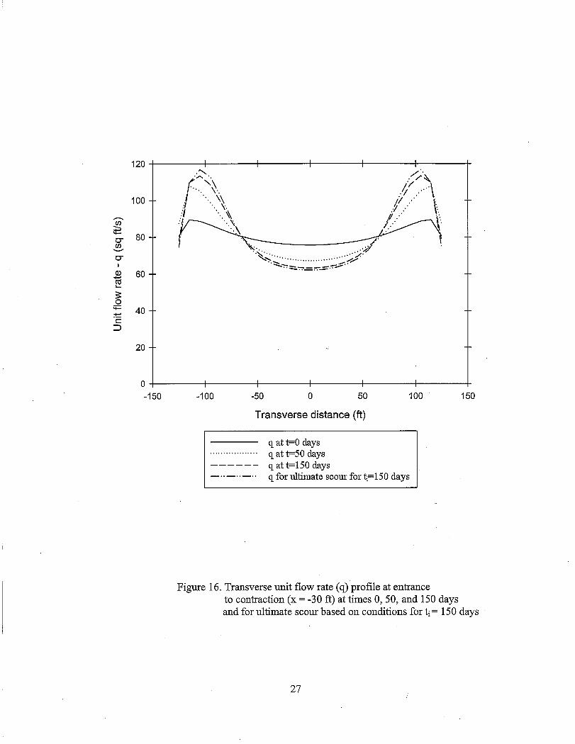
Figure 16. Transverse unit flow rate (q) profile at entrance to contraction (x = -30 ft) at times 0, 50, and 150 days and for ultimate scour based on conditions for ti = 150 days .................... .27

Figure 17. Maximum scour depth along centerline over time and ultimate scour based on conditions for ti = 150 days ........................ 2~

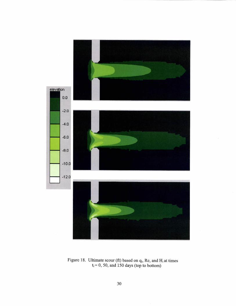
Figure 18. Ultimate scour (ft) based on qi, Re, and Hi at times ti = 0, 50, and 150 days (top to bottom) ............................................. 30

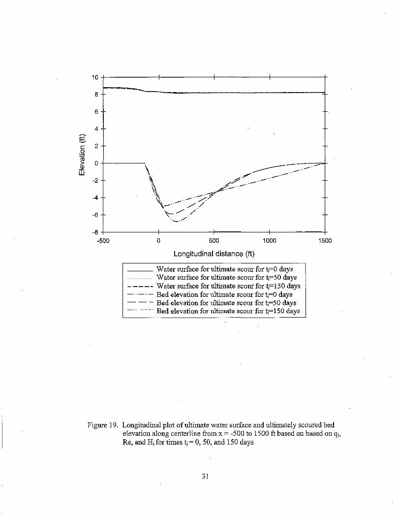
Figure 19. Longitudinal plot of ultimate water surface and ultimately scoured bed elevation along centerline from x = -500 to 1500 ft based on based on qi, Re, and HJor times ti = 0, 50, and 150 days ....................... 31

Figure 20. Transverse plot of ultimate water surface and ultimately scoured bed elevation at entrance to contraction (x = -30 ft) based on qi, Re, and Hi for times ti = 0, 50, and 150 days ....................... 32

Figure 21. Maximum scour along centerline over time for varied time step size ......... 34

Figure 22. Maximum scour along centerline over time for varied times step size using the second order Euler correction method ............................. 36

Figure 23. Longitudinal plot of friction factor at t = ° along centerline calculated based on the Henderson formula; smooth versus rough cases ................... 38

Figure 24. Maximum scour along centerline over time for smooth and rough cases using Henderson formula for calculating f ..................... 39

Figure 25. Longitudinal plots of friction factor at t = ° along centerline calculated based on Henderson versus Swamee-Jain formulas for calculating f ......... ..41

Figure 26. Comparison of maximum scour along centerline over time using Swamee-Jain explicit and Henderson implicit formulas to compute the friction factor. ....................................................... .42

VI

1. INTRODUCTION

1.1 Purpose

Two-dimensional hydraulic modeling can provide a more comprehensive and

realistic view of riverine hydraulics at bridge sites to help account for the threat of scour

in contracted bridge reaches. The Finite Element Surface-Water Modeling System: Two­

Dimensional Flow in a Horizontal Plane (FESWMS or FESWMS-2DH) was developed

especially for modeling "complex hydraulic conditions" such as those existing at bridge

sites where traditional one-dimensional techniques "cannot provide the needed level of

solution detail" (Froehlich, 1996, page 1-1 of the original reference). Whereas one­

dimensional research by Gaven et al. (2002) assumed a uniform flow distribution in the

contraction, two-dimensional modeling accounts for the nonuniform nature of the flow in

the horizontal plane. The FESWMS program within the Surface-Water Modeling System

(SMS) 7.0 software package developed at Brigham Young University is being used in

bridge design and research. Hydrologic Engineering Center Research Document No. 42

(RD-42), titled "Flow Transitions in Bridge Backwater Analysis," has shown with the

RMA-2 [mite element model, a model very similar to FESWMS and also available in the

SMS 7.0 software package, that two-dimensional modeling can provide a high degree of

correlation with actual field conditions (Hunt and Brunner, 1995). Aside from RD-42,

research in the area of two-dimensional hydraulic computer modeling of contractions has

been limited. The purpose of this study is to extend the clear-water contraction scour

research presented by Gaven et al. (2002) based on one-dimensional modeling.

1

1.2 Choice of Base Case

A contraction with vertical abutments similar to those in RD-42 (Runt and

Brunner, 1995) was chosen as a starting point for the present study. A Manning's

roughness coefficient (n) of 0.02, characteristic of a channel with a relatively smooth

boundary, was chosen for the base case. The kinematic eddy viscosity (Vo), which

accounts for the effects oflateral momentum transfer in the model, was set at 10 ft2/sec;

SMS documentation suggests a value of 5-50 ft2/sec. Further discussion of these choices

for the material properties is given in the first author's Masters thesis (McLean, 2002).

Figure 1 depicts the base case geometry and boundary conditions. A floodplain

width (B) of 1000 ft was consistently used for the transition sections upstream and

downstream of the contracted reach. The lengths of the upstream and downstream

reaches were always set at five times the floodplain width (5B). For the base case,

abutments had a 45-degree bevel that cut off 40 ftin length (a) and width (a) from each

abutment comer creating a more gradual entrance and exit geometry. The length of the

contracted section for the base case was determined by the abutment length (I), which

was set at 140 ft. The midpoint of the contraction is set as the origin, x = 0 ft, y = 0 ft.

The contraction width (b) was set at 250 ft for the base case, resulting in a contraction

ratio (bIB) of 1:4. The two boundary conditions, flow rate (Q) and downstream water

depth (Ro), were set at 20,000 cfs and 8 ft respectively. For this study, the flow rate and

downstream water depth were kept constant for all time steps. In general, however, it is

possible to change these boundary conditions in the model at each time step. The channel

bed starts out flat but changes over time based on the chosen soil's erosion

characteristics.

2

1=140' ~ ....... ....... ./

/\ ,

" /

YLx 1'-. Q = 20,000 efs

> B = 1000' b = 250'

a=40'1 ~ ~ \1/

/ !' ", '\ rr-a =40'

375'

\1 \ l/

(

Figure 1. Base case SMS model geometry and boundary conditions

3

The properties of the cohesive soil used in this report correspond to those of Soil

No.1 used in GUven et aL (2002), based on the original Erosion Function Apparatus

(EFA) data of Briaud et aL (2001). For Soil No.1, a low plasticity clay soil:

Critical shear stress (Tc) = 0.0572 Ib/ft2 =:= 2.74 N/m2

The scour rate (Sj ) = 1.936 (ft/day)/(1b/ft2) = 0.51 (mmlhr)/(N/m2)

1.3 Model Behavior

The distribution of velocity, depth, and flow rate per unit width in the channel

were of particular interest because of their effects on scour patterns at bridge sites.

Distributions of the velocity, depth, and flow rate per unit width (unit flow rate),

calculated for the base case with a flat bed, are depicted in Figure 2. Relatively little

change in velocity or depth occurs in the region upstream of the contraction. As the flow

enters the contraction, velocity increases, while a corresponding decrease in depth occurs.

The unit flow rate (the product of velocity and water depth) is high along the abutments

at the entrance to the contraction, and then in the center of the channel further

downstream as the flow is forced towards the center along the beveled entrance. The

actual depth is mainly dependent upon the boundary conditions Q and Ho, and the

velocity retarding parameters nand Vo. The jet-like behavior at the exit of the

contraction creates a distinct separation zone on each side of the channel between the

main flow and the eddy zones behind the abutments. The effect of lateral momentum

transfer and bed shear stresses results in a reduction of the velocity, expansion of the

main flow jet, and eventually reattachment of the flow to the side boundaries.

4

Velocity (ft/s)

14.0

12.0

10.0

8.0

6.0

4.0

2.0

0.0

Depth (ft)

/ / / / /

Unit flow rate (sq ft/s)

Figure 2. Velocity, depth, and unit flow rate distribution for the base case

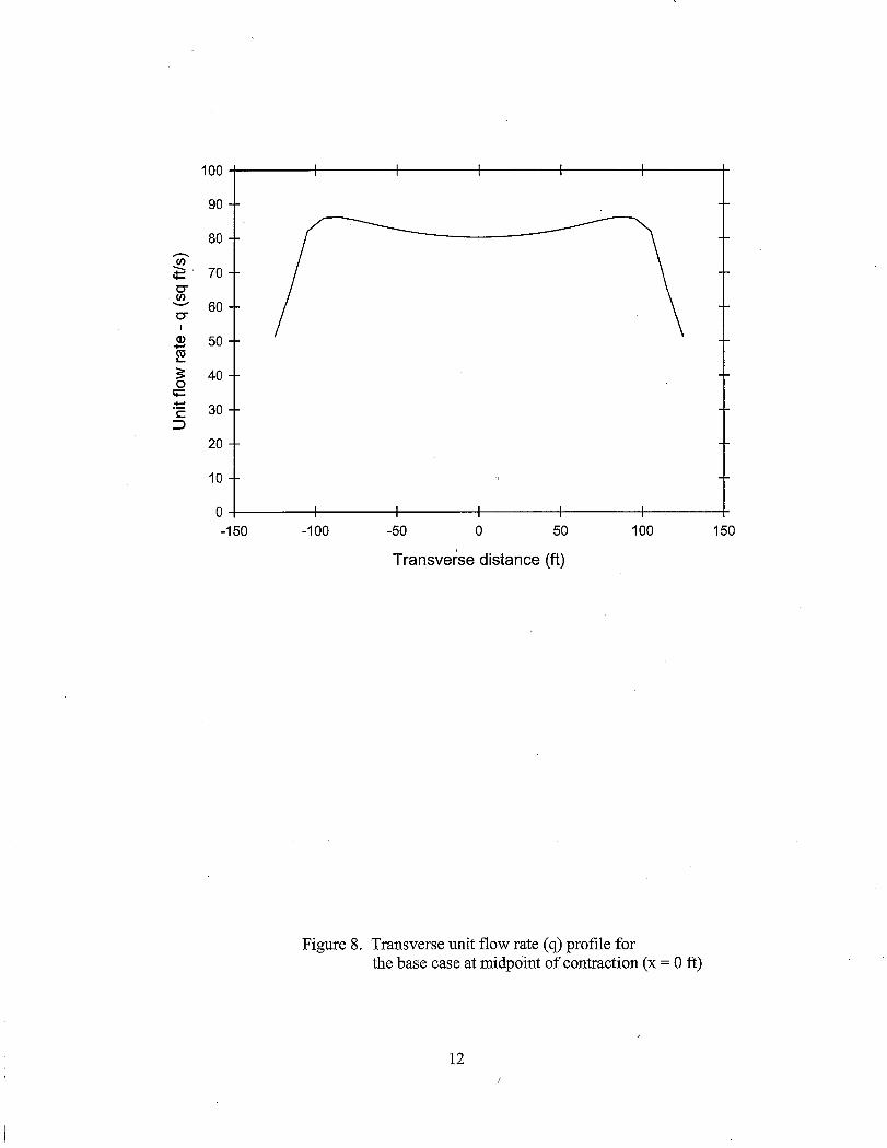
The effects of the contraction geometry on the hydraulic behavior for the base

case are visible in the transverse velocity, depth, and unit flow rate profiles. Figures 3, 4,

and 5 depict these profiles at what will be referred to as the contraction entrance (x = -30

ft) and Figures 6, 7 and 8 depict them at the midpoint of the contraction (x = 0 ft).

Velocity peaks are noticeable near the side boundaries as a result of the large amount of

flow that is diverted along the 45-degree beveled entrances and forced towards the center

of the contraction. Further upstream in the contraction, these peaks occur closer to the

boundary, and further downstream, they occur closer to the center of the channel. The

. transverse unit flow rate profiles show the flow concentrating towards the center of the

channel after entering the contraction.

6

14

13

12

..-.. (/)

.~ 11 .......... >-..... ·0 0 10 CD >

9

8

7 -150 -100 -50 0 50 100

Transverse distance (ft)

Figure 3. Transverse velocity profile for the base case at entrance to contraction (x = -30 ft)

7

150

-. ~ .......... c 0

:;::; co > Q)

UJ

10+--------r------~r_------~------_+--------r_------_r

8

6

4

2

o --------------------------------

-150 -100 -50 o 50 100

Transverse distance (ft)

Water surface elevation -- -- -- Bed elevation

Figure 4. Transverse bed and water surface profiles for the base case at entrance to contraction (x = -30 ft)

8

150

/

100

90

80 ...-.

~ 70 0-(J) -- 60 0-

CD 50 ...... Ci1 .... :s: 40 0

ti= :!: 30 c: ::J

20

10

0 -150 -100 -50 0 50 100

Transverse distance (ft)

Figure 5. Transverse unit flow rate (q) profile for the base case at entrance to contraction (x = -30 ft)

~

9

150

14

13

12

..-..

~ 11 "--'

~ ·0 0 10 Q)

> 9

8

7 -150 -100 -50 0 50 100

Transverse distance (ft)

Figure 6. Transverse velocity profile for the base case at midpoint of contraction (x = 0 ft)

10

150

1o+-------~--------~------4--------+--------~------~

8

........ 6 ¢:: -c 0

:;::; ctl 4 > Q)

ill

2

o -------------------------------

~150 -100 -50 o 50 100 150

Transverse distance (ft)

Water surface elevation - -- -- Bed elevation

Figure 7. Transverse bed and water surface profiles for the base case at midpoint of contraction (x = 0 ft)

11

100

90

80 ..-... en ~. 70 c-en ........- 60 c-

O> 50 ...... ro .... ?; 40 0

tt= ~ 30 c::: :::>

20

10

0 -150 -100 -50 0 50 100 150

Transverse distance (ft)

Figure 8. Transverse unit flow rate (q) profile for the base case at midpoint of contraction (x = 0 ft)

12

2. SCOUR CALCULATIONS METHODOLOGY

2.1 Time Dependent Scour Calculation Method

The time dependent nature of scour is important to consider when calculating

scour, especially in cohesive soils where scour may take much longer to develop than in

non-cohesive settings. The "scour rate in cohesive soils" (SRICOS) method, introduced

by Briaud and his colleagues at Texas A & M University for bridge pier scour, was

extended by Giiven et al. (2002) to account for contraction scour. Giiven et al. (2002)

presented a one-dimensional approach to modeling time dependent clear-water

contraction scour in a cohesive soil based on the SRICOS method. While Giiven et al.

(2002) investigated a contraction with a uniform flow distribution using a one­

dimensional model, the present study employs two-dimensional modeling to investigate

the effects of nonuniform flow at a contraction. At each time step, the two-dimensional

procedure was used to calculate scour for each node, or coordinate, in the model. Then

the scour was subtracted from the starting bed elevation to yield an updated streambed.

The procedure is to run the FESWMS model in SMS with the starting bed elevation, flow

rate, and contraction geometry. The SMS output file gives you velocity (V), water depth

(H), and water surface elevation at each node. In the SMS data calculator, these

parameters can be used to compute the time dependent scour based on the method

described below.

The Henderson implicit formula can be used to calculate f in an iterative fashion.

The formula is

13

f = 0.25

[10 (~+~)]2 g 12H Re.J[

f = friction factor

ks = roughness height

H = flow depth

Re = Reynolds number = 4q v'

q = unit flow rate = VH

v = magnitude of velocity

v = kinematic viscosity of water = 1.06*10-5 fe /s at 70° F

(1)

(2)

Iteratively solving for the friction factor requires an initial value of f for the first •

iteration. The Swamee-Jain explicit formula, originally for pipe flow, can be used to

obtain an initial estimate for the value of f:

f = 0.25

[log(~+ 5.74 )]2 3.7 ReO.9

kr = ksl(4H)

(3)

(4)

Subsequent values of f are calculated using the Henderson formula. For this

model, the percent change betWeen the 2nd and the 5th iterations was less than 1 % for each

node, so five iterations was chosen as a more than sufficient approximation of f.

The friction factor is then used to calculate the shear stress at each node in the

model:

14

(5)

1 = bed shear stress

p = density of water = 1.94 slugs/fe at 70°F

For Soil No.1, which was found to have a linear erosion function, the rate of

scour (R) in units oflength/time can then be calculated by mUltiplying the slope of the

erosion function (Si) by the difference in the bed and critical shea,r stress values. The soil

erodability information (Si and 10

) can be obtained from Erosion Function Apparatus

(EFA) tests. (For more information, see Briaud et aL (2001) and web pages:

http://tti. tamu.edu/ geotech/scour/ & http://tti. tamu.edu/ geotech/scour/efa _ overview.pdf).

The rate of scour is calculated as

R = Si *max(O, (1-1J) (6)

1 = bed shear stress

1 c = critical shear stress

The "max" function chooses the maximum value from the values inside the

parenthesis set apart by a comma, 0 and (1-10

), If the bed shear stress is less than critical

then the rate of scour is zero. Using the rate of scour, the incremental scour (~S) can be

calculated for the desired time step.

~S = R * Time Step (7)

The new bed elevation can be calculated by subtracting the scour that occurs

15

/

during the specified time interval from the bed elevation at the beginning of the interval:

New Bed Elevation = Bed Elevation - i1S (8)

Next, use the "save as" option to save the model with a new name. For the new

file you have created, select the New Bed Elevation as your Bed Elevation for the new

time step and give it a name. To do this, use the "Map Elevation ... " option under the

"Data" pull-down menu in the mesh module. Now, you can delete your old data files

except for the current elevation file and restart the process by running the model again.

This procedure can be performed in a sequential fashion to arrive to any time using any

time step size.

2.2 Ultimate Scour Calculation Method

Scour, or erosion of bed material, occurs when the shear stress acting on the bed is

greater than the critical shear stress for the bed material. For c1ear-'water scour, the

increase in flow area results in a decrease in the velocity and a coinciding decrease in bed

shear stress. Eventually, the depth of the scour hole will increase until the bed shear

stress is no longer sufficient for scouring to continue; this depth will be referred to as the

ultimate scour depth (referred to as "maximum scour depth" in Guven et al. (2002)). The

ultimate scour depth, or ultimate scour, corresponding to a particular and constant unit

flow rate (qi=ViHi) can be calculated at each node in the model for a particular time (ti),

where Vi and Hi are the magnitude of the flow velocity and the flow depth at that

particular time.

The following procedure was used to calculate the ultimate scour based on the output

16

from SMS modeling. The friction factor was calculated in the manner described in

section 2.1 using the Swamee-Jain formula as an initial estimate, and the Henderson

formula to iteratively come to a good approximation of f.

Equation (5) presented in section 2.1 for the calculation of shear stress can be

rearranged to solve for H. If the shear stress is set to be the critical shear stress, then the

/

depth that is solved for is the ultimate water depth that will occur before scouring ceases.

This depth will be called Hult.

2 2 pq. ( ) Hult =_'_f Re,ks,Hult 8'tc

(9)

For equation (9), Hult was originally solved in an iterative fashion since the

friction factor is a function of the ultimate depth. Hult was initially solved based on the

friction factor calculated from the initial depth (Hi) at the chosen time step.

(10)

Once an initial value for Hult has been calculated, the friction factor is then

recalculated iteratively as previously described. The Reynolds number is not

recalculated, in other words, q is assumed to stay constant. Five iterations were

performed to arrive at the final value of Hult. After the iterations were performed, a check

comparing the fifth iteration to the initial calculation of Hult based on the initial depth (HD

indicated that there was essentially no difference in the ultimate water depths (the

differences were less than 0.01 ft). Accordingly, Hult was plotted based on that initial

calculation, which used Hi to calculate f, since iterating did not yield an increase in

accuracy of Hult but did take a substantial amount of time.

17

The scour depth (SuIt,D corresponding to the ultimate water depth can be

realistically estimated by applying an energy equation to take into account the change in

velocity head that occurs during the development of the scour. The assumption of a

constant total head outlined in Gaven et aI. yields the following equation (Gaven et aI.,

2001, page 3-4 of the original reference):

(11)

Hi = flow depth at time ti

g = gravitational constant (32.2 ft/s2)

Positive SuIt,i (scour depth) values resulting from Equation (7) correspond to areas

where scouring occurs, while negative values correspond with low shear stress areas

where no scouring occurs and the bottom depth remains unchanged. As a result, negative

SuIt,i values had to be reassigned a value of zero in order to indicate that no scouring

occurred at these locations. Reassigning a scour depth of zero to these locations was

done using the maximum value function in the data calculator. The remaining positive

SuIt,i values represent the additional scour to the existing bed (at time ti) from which qi,

Re, and Hi were obtained. The ultimately scoured bed elevation is calculated as follows:

Ultimately Scoured Bed Elevation = Bed Elevation at time ti - Sult,i (12)

18

3. RESULTS AND DISCUSSION OF SCOUR CALCULATIONS

3.1 Time Dependent Scour Results

The base procedure for the calculation of time dependent scour was to use I-day

time steps up to a time of 50 days and 10-day time steps from 50 up to 150 days, to use

the Henderson implicit fonnula for open channel flow to calculate the friction factor (t),

and to assume a smooth boundary with a roughness height equal to zero (ks = 0 ft). A

contour plot of the bed shear stress for the base case model at time zero is depicted in

Figure 9. Figure 10 depicts the bed elevations at times 10,50, and 150 days. Water

surface and bed elevation plots along the longitudinal centerline are depicted for times of

50, 100, and 150 days in Figure 11; also shown is the ultimate scour based on the qi, Re,

and Hi for ti = 150 days. Plots of the unit flow rates (q) along the longitudinal centerline

for those times, as well as the unit flow corresponding to the ultimate s,cour based on the

conditions at ti = 150 days, are given in Figure 12. Transverse plots of the same

parameters are given in Figures 13 and 14, respectively, for the cross-section at the

midpoint of the contraction (x = 0 ft) and Figures 15 and 16 forthe entrance of the

contraction (x = -30 ft). In each figure, the base procedure was used to calculate the

scour over time. The ultimate scour was calculated based on the procedure in section 2.1.

Figure 17 shows the maximum scour along the centerline versus time with data points

taken at lO-day intervals out of the available data (I-day intervals for days 1-50, and 10-

day intervals for days 50-150). The maximum scour along the centerline is the lowest

bed elevation along the centerline of the long axis for a particular time. The ultimate

scour depicted is the lowest bed elevation along the centerline for the ultimately scoured

bed based on the qi, Re, and Hi for ti = 150 days.

19

0.30C

0.267

0.233

0.20C

0.167

0.133

0.1 OC

0.067

0.033

O.OOC

Figure 9. Distribution of bed shear stress (Ib/ft2) for the base case at time t = 0

20

elevation

I"-2.0

-4.0

-6.0

-8.0

-10.0

-12.0

Figure 10. Bed elevation (ft) contours at times t = 10, 50, and 150 days (top to bottom)

21

......... ¢: ......... c 0

:;::. CO > Q)

w

12

10

8

6

4

2

0

-2

-4

-q

-8

----_. ~.~~====~-=~=.~~=-=-================~

-1--------" - - - - - - - - - - - --=-....:=~-=---t-

-500 o 500

Longitudinal distance (ft)

1000 1500

----- Water smface t=o days ------ -. ------- .. - Water smface t=50 days - - - - - - Water smface t=150 days - --_. -- .. Water smface for ultimate scotu" for t=150 days - - - Bed elevation t=o days - . -. -. - Bed elevation t=50 days - - - - Bed elevation t=150 days ----- Bed elevation for ultimate scam for t=150 days

Figure 11. Longitudinal plot of water surface and bed elevation. along centerline from x = -500 to 1500 ft at times 0, 50, and 150 days and for ultimate scour based on conditions for ti = 150 days

22

-en ¢:! cr en ....... cr

Q.) +-' ctl ..... :;: 0

;:;:: ~ c::

::>

100+------------+------------r------------r-----------+

80

60

40

20

o +-----------~------------_r------------+_----------_+ -500 o 500

Longitudinal distance (ft)

q at t=o clays qat t=50 days qat t=150 days

1000

q for ultimate scour for 1:,=150 days

Figure 12. Longitudinal plot of unit flow rate (q) along centerline from x = -500 to 1500 ft at times 0, 50, and 150 days and for ultimate scour based on conditions for ti = 150 days

23

1500

10

8

6

4

...-. ~ 2 .......... c 0

0 :0:; ct! > CD -2 ill

-4

-6

-8

-10

-150

--'-'-'-'-'--/~. .~.~

-100 -50 o 50 100

Transverse distance (ft)

----- Water smiacet=O days -... _- -. .. . . .. . .. Water smiace t=50 days - - - - - - Water smiace t=150 days - .. _ .. _ .. Water smiace for ultimate scom for t.=150 days - - - Bed elevation t=o days -. -- - -- Bed elevation t=50 days - - - - Bed elevation t=150 days ----- Bed elevation for ultimate scom for t.=150 days

Figure 13. Transverse bed and water surface profiles at midpoint of contraction (x = ° ft) at times 0, 50, and 150 days and for ultimate scour based on conditions for ti = 150 days

24

150

......... en ¢: 0-en

'-'"

0-

Q) ...... e? :s: 0

I:j:

:!: C

::::>

120+--------r-------+--------r-------~------_r------_+

100 /./~ . . J' \ /1 ... ······ ..

:/ .. ' \ // .' '. ,. . . .

80

60

40

20

o +--------+--------+--------r--------r--------r------_+ -150 -100 -50 o 50

Transverse distance (ft)

q att=O days q at t=50 days qat t=150 days q for ultimate scom for 1:,=150 days

100

Figure 14. Transverse unit flow rate (q) profile at midpoint of contraction (x = 0 ft) at times 0,50, and 150 days and for ultimate scour based on conditions for tj = 150 days

25

150

10

8

6

4

........ 2 ~ ......... c 0 0

:;::::; co -2 > (].)

ill -4

-6

-8

-10

-12 -150

.. ' ~

-'_'-'-0_°-

-100 -50 o 50 100

Transverse distance (ft)

----- Water smface t=o days .... _ ............ Water smface t=50 days - - - - - - Water smface t=150 days _ .. _ .. _ .. Water smface for ultimate SCOlU" for 1i=150 days - - - Bed elevation t=o days -. _. - . - Bed elevation t=50 days - - - - Bed elevation t=150 days ----- Bed elevation for ultimate scom' for 1i=150 days

Figure 15. Transverse bed and water surface profiles at entrance to contraction ex = -30 ft) at times 0, 50, and 150 days

and for ultimate scour based on conditions for tj = 150 days

26

150

-. en ~ 0-en '-'"

0-

0> ..... ~ ~ 0

q:: :t:: C

=>

120+-------~------~------_+------_4--------~------+

100

80

60

40

20

/;-~ // .. \ '; .. /I...... t.

.'! . . /..... .. ••..

0+-------~------_4--------+_------~------_4------__+

-150 -100 -50 o 50

Transverse distance (ft)

q at t=o clays qat t=50 days qat t=150 days

100

q for ultimate scom for 't.j=150 days

Figure 16. Transverse unit flow rate (q) profile at entrance to contraction (x = -30 ft) at times 0,50, and 150 days

150

and for ultimate scour based on conditions for ti = 150 days

27

0

-1

-2

...--. ~ -3 '-"

c 0

:;::::; co

-4 > Q)

W

-5

-6

-7

0

Ultimate scour __ _

20 40 60 80 100 120 140 160

Time (days)

• Maximum scour - - - Ultimate scour based on tj=150 days

Figure 17. Maximum scour depth along centerline over time and ultimate scour based on conditions for ti = 150 days

28

3.2 Ultimate Scour Results

The ultimate scour was calculated based on the qi, Re, and Hi at times 0, 50, and

150 days. One-day time steps were chosen to reach 50 days and 10-day time steps were

used between days 50 and 150. Basing the ultimate scour on the data fot: the 150-day

case gives a more accurate representation of the ultimate scour depths that may occur

rather than basing it on the data for an earlier time. As time goes on, the scouring of the

bed results in changes in the flow pattern which dictate where subsequent scour will be

most concentrated. Plan views of the ultimately scoured beds, based on the times

mentioned previously in this section, are depicted in Figure 18. Longitudinal profiles of

the ultimately scoured beds and corresponding water surface elevations based on times ti

= 0,50, and 150 days are shown in Figure 19. The transverse profiles of the same

features are depicted in Figure 20 for the entrance of the contraction (x = -30 ft).

29

elevation

10.0

-2.0

-4.0

-6.0

-3.0

-10.0

-12.0

Figure 18. Ultimate scour (ft) based on qi; Re, and Hj at timesti= 0, 50, and 150 days (top to bottom)

30

..-.. ¢:: '-"

c 0

:;::; co > Q)

W

10

8

6

4

2

0

-2

-4

-6

-8 -500

. \ ----.~- .. -.. -'l .;:r -"-~ A _., ., ~y .. -., \\. /_ .. -\ _ .. _ .. -;;:7 _., //

. /' /'

o

~ . ._ . ./ 500

Longitudinal distance (ft)

1000

___ Water surface for ultimate scom for 1:;=0 days .... . ... ..... . Water surface for ultimate scam for 1:;=50 days ----- Water surface for ultimate scam for 1:;=150 days _ .. _ .. - Bed elevation for ultimate scom for 1:;=0 days - - - Bed elevation for ultimate scom for 1:;=50 clays _. - . _. Becl elevation for ultimate scom for 1:;= 150 days

1500

Figure 19. Longitudinal plot of ultimate water smface and ultimately seamed bed elevation along centerline from x = -500 to 1500 ft based on based on qi, Re, and Hi for times ti = 0, 50, and 150 days

31

-S c 0

:;::; co > Q)

W

10

8

6

4

2

0

-2

-4

-6

-8

-10

-12 -150

~.

.--~~'==,: --':--" ~:::2":. -" _ .. - .. .:::-:-: ~"-

.. -.. ;;), "- .. -. ~ .. -.. :--- // .~" -.. -.. ~ \ / / \ " .1 \/ / \ "'-J ~ .f \ ) ./ ,. -100 -50 o 50 100

Transverse distance (ft)

___ Water surface for ultimate scam for 11=0 days .............. Water surface for ultimate scom for 11=50 days - - - - - Water surface for ultimate scam for 11= 15 0 days _ .. _ .. - Bed elevation for ultimate scom for tFO clays - - - Bed elevation for ultimate scam for 1:;=50 days _. - . _. ,Bed elevation for ultimate scour for 11=150 days

150

Figure 20. Transverse plot of ultimate water surface and ultimately scoured bed elevation at entrance to contraction (x = -30 ft) based on based on qi, Re, and Hi for times ti = 0,50, and 150 days

32

4. FURTHER INVESTIGATIONS INTO METHODOLOGY

The next analyses look at varying the time step size, using a second order

correction method in the modeling procedure, comparing the smooth case (ks = 0 ft) to a

rough case (ks = 0.000974 ft), and comparing the Henderson implicit formula for open

channel flow to the Swamee-Jain explicit formula for pipe flow for calculating f.

4.1 Effect of Time Step Size

The calculation of a scour rate allows the modeler to calculate the scour that is

expected to occur over a specified time interval. The size of that time interval may be

dictated by flow information available; daily flow data are available through the United

States Geological Survey (USGS) for many streams and rivers. In this analysis, time

intervals of 1,5, 10 days were used to approach the scour that would be realized after 50

days of flow. The maximum scour along the centerline was plotted in Figure 21 for each

case, with these data points being retrieved at 10 days intervals as before. These plots are

labeled uncorrected in reference to the next section which sets forth a method for

adjusting the model with a second order Euler correction. Naturally, smaller time steps

will provide a more accurate approach to determining the time dependent scour. Even so,

after 50 days, the difference in the bed elevation is less than 0.5 ft when comparing the 1

and 10-day time steps.

4.2 Effect of Second Order Correction

A second order correction (corrected method) was performed to compare with

thus far presented first order calculations (uncorrected). In the previous calculations, the

initial model with a given bed elevation is run. Then, the data calculator is used to

calculate the friction factor, shear stress, rate of scour (rate), and the scour occurring over

33

-¢::: -c: 0

:.0:: ctS > CD W

b~------~------~------~------~-------+-------+

-1

-2

-3

-4

\;. \". , ... , ... , ... , ... , ... , ...

, O. , . ~" ...... .

" " ·0 " . " ~ ...... ............

...... . .. ......... ..... . ............ ·····0 ...... ..

................ . ... ............... ······0 ..........

..... ~

-5+--------r-------+------~r_------+_------~------_+

o 10 20 30

Time (days)

40

-e-- Time step = 1 day (uncorrected) ····0··· Time step = 5 days (uncorrected) -~- Time step = 10 days (uncorrected)

50 60

Figure 21. Maximum scour along centerline over time for varied time step size

34

a specified time interval for that rate using the first order Euler approximation:

New Bed Elevation = Initial Bed Elevation - (Initial Rate of Scour * Time Step)

(13)

The correction method is more intensive requiring that the model be run again

with this new bed elevation, and that the same calculations be performed for the new

output. However, rather than calculate the new bed using the method described above, a

second order Euler approximation is now used which employs the rate and elevation from

the initial model to obtain a more accurate approximation of the new bed elevation. The

following equation describes this second order approximation:

New Bed Elevation =

I .. 1 B dEl . (( Initial Rate + New Rate )*T· S )" mba e evatlOn - lme tep . 2

(14)

Figure 22 depicts varied time step sizes for the corrected case calculated using this

second order approximation. Time step size is less important for when the correction is

used. Although the UIicorrected I-day time step plot is not included in this plot for

considerations of clarity, it lies virtually on top of the corrected I-day time step plot. As

expected, the smaller the time step, the closer the corrected and uncorrected plots. Since

the uncorrected method requires about half as much time as the corrected, and since 1-

day flow data is commonly available, the uncorrected I-day case was used for analyses in

this study.

35

-¢:: '-'"

c 0

:;::; co > Q)

ill

oe-------4-------~------_r------_r------_+------_+

-1

-2

-3.

-4

-5+-------~--------~------~--------~--------r_------_r

o 10 20 30

Time (days)

40

___ Time step = 1 day (corrected) ····0··· Time step = 5 day (corrected) -~- Time step = 10 days (corrected)

50 60

Figure 22. Maximum scour along centerline over time for varied time step size using the second order Euler correction method

36

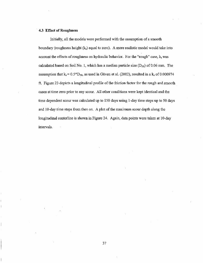
· 4.3 Effect of Roughness

Initially, all the models were performed with the assumption of a smooth

boundary (roughness height (ks) equal to zero). A more realistic model would take into

account the effects of roughness on hydraulic behavior. For the "rough" case, ks was

calculated based on Soil No.1, which has a median particle size (D50) of 0.06 mm. The

assumption that ks = 0.5*D50, as used in Giiven et al. (2002), resulted in a ks of 0.000974

ft. Figure 23 depicts a longitudinal profile of the friction factor for the rough and smooth

cases at time zero prior to any scour. All other conditions were kept identical and the

time dependent scour was calculated up to 150 days using I-day time steps up to 50 days

and 10-day time steps from then on. A plot of the maximum scour depth along the

longitudinal centerline is shown in Figure 24. Again, data points were taken at 10-day

intervals.

37

'I-L-a ...... u ~ c a U ·c LL.

0.0090

0.0088

0.0086

0.0084

0.0082

0.0080

0.0078

0.0076

0.0074

0.0072

0.0070

0.0068 -6000 -4000 -2000 o 2000

Longitudinal distance (ft)

-- Henderson smooth ........ Henderson rough

.....

4000 6000

Figure 23. Longitudinal plot of friction factor at t = 0 along centerline calculated based on the Henderson fonnula; smooth versus rough cases

38

........ ¢:: "'-'

c 0

:;::::; co > Q)

W

0

-1

-2

-3

-4

-5

-6

-7

-8

0 20 40 60 80

Time (days)

_ Smooth

···0·· Rough

100 120 140 160

Figure 24. Maximum scour along longitudinal centerline over time for smooth and rough cases using Henderson formula for calculating f

39

4.3 Effect of Swamee-Jain Explicit Formula Versus Henderson Implicit Formula to

Calculate f

In the section that discusses the calculation of time-dependent scour, a method is

proposed to calculate the friction factor f employing both the Swamee-Jain explicit

formula and the Henderson implicit formula. The proposed method uses Swamee-Jain as

an initial estimation of f to be used in subsequent calculations using the Henderson

formula, which calculates f as a function of f. The Henderson formula is then used to

calculate f in an iterative fashion; this method is referred to as Henderson. To conserve

steps and time, the use of the Swamee-Jain explicit formula alone as a fairly accurate

estimate of f was investigated. Figure 25 is a plot of f along the longitudinal centerline

for the base case prior to scouring calculated using the two different methods. Then, an

analysis was done using the same time step and data point retrieval scheme as the

previous sections in this chapter. The two methods to compute f are compared in Figure

26.

40

..... ..... 0

1:5 ~ c: 0 :g .;:: LL.

· 0.0090 +--f--f--f--I--f--f--f--I--f--f--f--I--+--+--+--t--+--+--+--j--+--+--+-+

0.0085

0.0080 . ........................................... .

0.0075

0.0070

0.0065

.. ' . ..... ....

0.0060 +--+--+--+--t--f---+---+--+-+--+--+--+--+---+----i----il-I-i-+-+-+-+-+-+

-6000 -4000 -2000 o 2000

Longitudinal distance (ft)

-- Henderson smooth ........ Swamee-Jain smooth

4000 6000

Figure 25. Longitudinal plots of friction factor at t = 0 along centerline calculated based on Henderson versus Swamee-Jain formulas for calculating f

41

0

-1

-2

..-.. ~ '-'" -3 c 0

:;::::; co > -4 <D

LU

-5

-6

-7

0 20

o.

40 60 80

Time (days)

100

_ Henderson smooth ···0·· Swamee-Jain smooth

120 140 160

Figure 26. Comparison of maximum scour along centerline over time using Swamee­Jain explicit and Henderson implicit formulas to compute the friction factor

42

5. CONCLUDING REMARKS

The methods described in this report allow for the calculation of time-dependent

scour with a user-defined time step. Flow data, variable or constant, can be used to

calculate scour and update the bed of the model. In addition, an ultimate scour can be

calculated based on the model results obtained for a particular time. The authors suggest

that the corrected method be used and that smaller time steps be used, at least initially

(since more scour occurs during this period). It is also suggested that the friction factor

be calculated with the Henderson formula, without ignoring roughness, since this

approach appears to be more realistic.

Physical modeling, comparison with field measurements, and comparison with

three-dimensional modeling are still needed to investigate whether two-dimensional

modeling is an accurate representation of complex three-dimensional hydraulics at bridge

sites.

43

REFERENCES

Briaud, J.L., F.C.K Ting, H.C. Chen, Rao Gudavalli, Suresh Perugu, Gengsheng Wei. "SRICOS: Prediction of Scour Rate in Cohesive Soils at Bridge Piers." Journal of Geotechnical and Geoenvironmental Engineering, Vol. 125, No.4, April 1999, pp. 237-246, American Society of Civil Engineers, Reston, Virginia, U.S.A.

Briaud, J.L., F.C.K Ting, H.C. Chen, Y. Cao, S.W. Han, and KW. Kawk. "Erosion Function Apparatus for Scour Rate Predictions." Journal of Geotechnical and Geoenvironmental Engineering, Vol. 127, No.2, February 2001, pp. 237-246, American Society of Civil Engineers, Reston, Virginia, U.S.A.

Froehlich, David C. "Finite Element Surface-water Modeling System: Two-dimensional Flow in a Horizontal Plane Version 2 Draft User's Manual." FHW A, U. S. Department of Transportation. 1996.

Giiven, Oktay, J.G. Melville, and J.E.Curry.- "Analysis of Clear-Water Scour at Bridge Contractions in Cohesive Soils." Interim Report No. 930-490, Highway Research Center, Auburn University, AL, June 2001.

Giiven, Oktay, J.G. Melville, and J.E.Curry. "Analysis of Clear-water Scour at Bridge Contractions in Cohesive Soils." Transportation Research Record No. 1797, Journal of the Transportation Research Board, pp. 3-10. 2002.

Hunt and Brunner. "Flow Transitions in Bridge Backwater Analysis." Research Document 42 (RD-42), Hydraulic Engineering Center, U.S. Army Corps of Engineers, Davis, CA, 1995.

McLean, Jacob P. "A Numerical Study of Flow and Scour in Open Channel Contractions". Thesis. Auburn University. http://www.1ib.auburn.edul (Library).

44