Biogeosciences, 9, 3323–3336, 2012www.biogeosciences.net/9/3323/2012/doi:10.5194/bg-9-3323-2012© Author(s) 2012. CC Attribution 3.0 License.

Biogeosciences

A two-dimensional model of the methane cycle in a sedimentaryaccretionary wedge

D. E. Archer1 and B. A. Buffett2

1Department of Geophysics, University of Chicago, USA2Department of Earth and Planetary Sciences, University of California, Berkeley, USA

Correspondence to:D. E. Archer (d-archer@uchicago.edu)

Received: 28 February 2012 – Published in Biogeosciences Discuss.: 14 March 2012Revised: 4 July 2012 – Accepted: 3 August 2012 – Published: 24 August 2012

Abstract. A two-dimensional model of sediment columngeophysics and geochemistry has been adapted to the prob-lem of an accretionary wedge formation, patterned after themargin of the Juan de Fuca plate as it subducts under theNorth American plate. Much of the model description isgiven in a companion paper about the application of themodel to an idealized passive margin setting; here we buildon that formulation to simulate the impact of the sedimentdeformation, as it approaches the subduction zone, on themethane cycle. The active margin configuration of the modelshares sensitivities with the passive margin configuration, inthat sensitivities to organic carbon deposition and respirationkinetics, and to vertical bubble transport and redissolution inthe sediment, are stronger than the sensitivity to ocean tem-perature. The active margin simulation shows a complex sen-sitivity of hydrate inventory to plate subduction velocity, withresults depending strongly on the geothermal heat flux. Inlow heat-flux conditions, the model produces a larger inven-tory of hydrate per meter of coastline in the passive marginthan active margin configurations. However, the local hydrateconcentrations, as pore volume saturation, are higher in theactive setting than in the passive, as generally observed in thefield.

1 Introduction

An accretionary wedge sediment complex is an example of a“structural” hydrate deposit, in which tectonics and gas flowplay obvious roles in controlling the abundance and distri-bution of methane hydrate, as opposed to the “stratigraphic”deposits (Milkov, 2004), in which sediment accumulates into

depositional layers. In an accretionary wedge complex, thesediment is actively deformed by compression associatedwith the scrape-off of the sediment complex from the under-lying subducting oceanic crust (Carson et al., 1990).

Structural deposits comprise a smaller fraction of the hy-drate inventory globally (Boswell and Collett, 2011), butform hydrate in higher concentrations, even forming mas-sive hydrate blocks. Hydrate is found closer to the sea floorthan in the stratigraphic deposits (Torres et al., 2002), whichtend to concentrate hydrate at the base of the stability zone,often hundreds of meters below the sea floor. Structural de-posits might therefore release carbon into the ocean or evenmethane into the atmosphere more quickly than the time con-stant would be for a response from the stratigraphic deposits.

Models of methane hydrate cycling have been applied toactive margin settings by driving them with increased upwardpore fluid flow (Buffett and Archer, 2004; Chatterjee et al.,2011; Luff and Wallmann, 2003). Here we attempt to inter-nalize the pore fluid flow into a methane hydrate sedimentarymodel by expanding the model domain to bedrock and into asecond dimension, perpendicular to the motion of the under-lying plate sliding into the subduction zone. In particular, themodel is applied to the case of the Cascadia margin (Spenceet al., 2000).

2 Overview of the passive margin configuration

Called SpongeBOB, the numerical model is described in acompanion paper (Archer et al., 2012) as it was formulatedfor a passive continental margin setting. The model formu-lation as described in that paper will be summarized herebefore we show details of the additional model formulation

Published by Copernicus Publications on behalf of the European Geosciences Union.

3324 D. E. Archer and B. A. Buffett: A two-dimensional model of the methane cycle

required for the accretionary wedge setting. The model is for-mulated on a two-dimensional grid, onshore/offshore in thelateral dimension and with a stretching “sigma” grid in thevertical. The model is intended to span the continental mar-gin from the continent to the abyss, over geologic time scalesof 107–108 yr.

2.1 Sediment transport

A sediment transport scheme distributes material to the seafloor. Continental material originates at the left-hand (conti-nental) side of the domain, and is transported and sedimentedaccording to the sinking velocities of the various grain sizes,and the water depth (which prevents sedimentation if it istoo shallow). Another fraction of the sedimenting materialis called “pelagic”, and it deposits uniformly throughout thedomain, if the water is deep enough. When the slope of thesea floor exceeds a critical value set at 4–6 % grade, sedimentresuspends and is distributed downslope. This material is as-sumed to carried to the abyssal floor in turbidity currents thatonly allow resedimentation to begin when the slope of thesea floor decreases offshore to less than 1 % grade (Meiburgand Kneller, 2010). The sedimentation scheme produces acontinental shelf, a well-defined shelf break, and a continen-tal slope. The various parameters of the sedimentation weretuned in order to reproduce the envelope of sediment: theshapes of the sea floor and the depth to bedrock.

2.2 Isostasy

Bedrock in the model floats isostatically, balancing the loadfrom the crust and sediment against that of a hypotheticaldisplaced mantle fluid. The buoyancy of the crust is affectedby cooling of the upper mantle in a thermal boundary layerthat thickens with the square root of time, allowing subsi-dence with increasing crustal age. The elevation of the crustrelaxes toward the equilibrium value on an isostatic reboundtimescale of 104 yr. The passive margin model has no repre-sentation of crustal rigidity except for a numerical smoothingoperation, which has a spatial range of 10–20 km.

2.3 Organic carbon and methane

The particulate organic carbon (POC) content of the con-tinentally derived sedimenting material is specified in themodel when it hits the sea floor, as a function of water depth.In the passive margin simulation, sea level changes were im-posed on the simulation, along with a correlated time-varyingoxygen “state” of the ocean, which drives changes in POCconcentration and the chemistry of the organic matter, mostnotably its H / C ratio. The active margin simulation reachessteady state in only 10 Myr, which is shorter than the 200 Myrduration of the passive margin simulations, so geological sealevel and ocean oxygenation changes are not imposed on thesimulations here. Instead, the relative sea level for these sim-ulations was varied by±20 m on a cycle time of 1 Myr, rep-

resenting local tectonic uplift and subsidence driven by theforces confronting the crust in this “turbulent” part of crustalgeophysics. The impact of this stipulation can be assessed ina simulation calledNo Sealevelwith time-invariant sea level.

Biologically and thermally driven chemical reactions pro-duce dissolved methane, CH4, which interacts with the gasand hydrate phases depending on temperature and pressureconditions. Respiration of POC first consumes pore watersulfate, SO2−

4 , until it is depleted, which occurs relativelyshallow in the sediment column. Bacterial respiration of POCthen produces CH4 and CO2. The maximum efficiency ofCH4 production from the organic carbon is set by redox bal-ance according to the H / C ratio of the POC. Porewaterδ13Cdata constrain the methanogenesis to be about 50 % of res-piration, which is a bit lower than the maximum set by theredox constraint, as if some of the molecular hydrogen in-termediary reacts with oxidized mineral phases rather thandissolved CO2 to produce methane.

As temperatures warm further, exceeding about 60◦C,petroleum is produced, if the H / C ratio in the POC exceedsa value of 1 (Hunt, 1995). Petrogenesis draws the H / C ra-tio down toward a value of 1. A fraction of this petroleum(10 %) is assumed to migrate upward with a velocity of 1 mper thousand years. If it reaches the biological zone (tem-perature less than about 50◦C), it can be respired, producingCH4 and CO2, similarly to respiration of POC.

Thermal methanogenesis begins at about 150◦C, pro-ducing CH4, dissolved CO2 species collectively called dis-solved inorganic carbon (DIC), and dissolved organic carbon(DOC). Ultimately, the CH4 production is limited by hydro-gen in the POC, with H / C approaching 0 in the hottest sed-iments. Thermogenic DOC production is produced in a sto-ichiometry of CH2O (e.g. acetate). DOC is also released by“sloppy feeding” in the respiration zone, and it is consumedin the respiration zone (producing DIC and methane if SO2−

4is not available) with the same rate constant as applied tomigrated petroleum. SO2−

4 and CH4 are also consumed byanaerobic oxidation of methane (AOM).

The CH4 concentration is compared with the solubility ofbubbles and hydrate, and allowed to form those phases if itexceeds supersaturation. Hydrate is stationary within the sed-iment but bubbles migrate, following an ad-hoc parameteri-zation that redistributes CH4 in bubbles into overlying gridcells. This parameterization was needed to prevent buildupof excessive bubble volumes throughout the deep sedimentcolumn, and, although the details of how the transport occursare sketchy and at any rate unresolved in the model, it seemsclear that, in the absence of evaporates or permafrost, mostmethane gas produced in the sediment column does manageto escape the sediment column eventually (Hunt, 1995).

When rising gas encounters undersaturated conditions inthe model, it redissolves following a simple exponentialfunction of height in the sediment column. The methane in-ventory was found to be extremely sensitive to the scaleheight in the parameterization, and we will show similar

Biogeosciences, 9, 3323–3336, 2012 www.biogeosciences.net/9/3323/2012/

D. E. Archer and B. A. Buffett: A two-dimensional model of the methane cycle 3325

sensitivity studies for the active-margin model with similarresults.

3 Active model configuration

3.1 Reference case and variants

To understand and document how the model works, we showresults from a suite of model sensitivity runs summarized inTable 1. Details of these scenarios will be explained as thenew components of the model relevant to the active marginsetting are described. In contrast to the passive margin sim-ulations, the grid resolution is the same for all of the activemargin simulations presented here.

3.2 Deformation of the sediment column

In the active model configuration, in addition to the pro-cesses in the passive margin model, the model grid in thehorizontal dimension is manipulated to simulate the uniformcompaction and thickening of the sediment column by lat-eral compression. Thex coordinate values of the grid cellsare carried laterally by the moving crust, and the spacing be-tween the grid points decreases, resulting in uniform verticalthickening of the sediment column.

The velocity of the incoming sediment column in the off-shore edge of the model domain (the right) is the crustal ve-locity, specified as a parameter of the model scenario (forwhich there are sensitivity runsPlate 100, 80, and20). Thebase plate velocity is taken to be 40 mm yr−1, from the sub-duction rate of the Juan de Fuca plate. The Juan de FucaRidge is neither orthogonal to the direction of plate mo-tion, nor is it geographically stationary, but rather is mov-ing slowly toward the trench. The model formulation as pre-sented here simplifies this geometry into two dimensions byequating the spreading and subduction velocities, maintain-ing a constant distance between the ridge and the subductionzone throughout the model simulation. This simplificationaffects the plate velocity and also the amount of sedimentthat enters the wedge through time, and its impact can be as-sessed from the sensitivity to plate velocity and to sedimen-tation (simulationPelagic).

At the onshore end of the domain, the sediment columnvelocity is held fixed at a value 10 times lower than the in-coming sediment column velocity, representing a sedimentcolumn nearly stopped by collision into the other plate. Therate is specified at an extrapolatedx location at which the seafloor would rise above sea level. The velocities (u) of the gridpoints offshore of this are determined by

usedcoln+1 = usedcoln − Kdeform1x

1zsedcol

(uplate− usedcoln

)(1)

whereKdeform is a dimensionless deformation constant thatcontrols the horizontal extent of the wedge relative to the

thickness of the incoming sediments. The velocities are neg-ative because they flow in the direction of decreasingx

(Fig. 1a). The horizontal extent of the deformation zone, inthis simulation about 150 km, is determined by the value cho-sen forKdeform (for which there is a sensitivity run calledWide Def).

The x coordinate (location in physical space) of each hor-izontal grid point is updated each time step according to itscalculated velocity. As the sediment column slides landward,the state of the underlying ocean crust at the grid point is re-calculated based on its new location, including in particularthe flexure effect of the subducting plate in the trench. Thesediment column rides but also isostatically steers the path-way of the subsiding ocean crust as it thickens.

As grid points move across thex = 0 origin, or as the sed-iment column begins to outcrop from the ocean, they aredropped from the model domain, and a new grid point is cre-ated on the far right-hand side of the domain. These sedimentcolumns are initialized with a computationally required min-imum 1 m thickness per each of 15 grid cells, a negligiblefraction of the ultimate sediment wedge. The 400 km markfrom the extrapolated coastline is taken to be the spreadingcenter where ocean crust is created and begins to accumu-late sediment. The grid points propagate through the domain,emerging on the right as new crust is formed at the spread-ing center, and accumulating sediment and deforming as theyconverge toward the left. The eventual model steady state hasno stationary points in it, but it manages to reach a movingstationary solution.

By conservation of volume, the thickness of the column1zsedcolincreases as1x decreases. The model is formulatedin vertical columns, which requires that the sediment columndeforms strictly vertically. The increasing vertical has the ef-fect of increasing the excess pressure in the fluid phase, driv-ing an expulsion fluid flow (Yuan et al., 1994). Real sedimentcolumn compression is generally focused on diagonal faultsin the column, with a block of sediment from one side of thefault over-riding the other by sliding upward along the fault.The faults can dip onshore (normal) or offshore (abnormal),perhaps depending on the frictional state of the contact withbedrock (Davis et al., 1983).

Fortunately, previous models of sediment accretion havefound a strictly vertical formulation to be an acceptable ap-proximation, for modeling heat flow (Wang et al., 1993) andmineral closure ages (Batt et al., 2001). The effect of slip mo-tion along diagonal faults dipping in either direction wouldbe to displace material laterally. A parcel of over-riding sed-iment over a fault dipping offshore, for example, would bemoving shoreward somewhat as it rides the wedge upwardtoward shallow waters through the domain of the model. Aparcel at the top of the undeformed incoming sediment col-umn might progress into the wedge a bit before a contem-poraneous parcel from the bottom of the incoming column.But the lateral displacements ought to be limited by typicalfault geometry to be not much larger than the thickness of

www.biogeosciences.net/9/3323/2012/ Biogeosciences, 9, 3323–3336, 2012

3326 D. E. Archer and B. A. Buffett: A two-dimensional model of the methane cycle

Table 1.Summary of the configurations of model scenarios.

Model Name Description

Base Baseline scenario

Bio 10 %Bio 100 %

Variation in the defined labile fraction of POC, 10 % and 100 % respectively, within the contextof the Base case which takes 50 %.

T − 2, T + 2, T + 4 Effect of ocean temperature, changes of−2◦C, 2◦C, and 4◦C.

No Bubb Mig Bubble migration disabled.

Bubb 100 mBubb 2 km

Bubble redissolution scale height of 100 m and 2 km, relative to the Base case of 500 m.

Plate 100, 80, 20 Plate subduction velocity of 100, 80, or 20 mm yr−1 instead of the Base case of 40 mm yr−1.The slowest plate simulation was spun up for 20 Myr instead of Base 10 Myr.

Broad Slope Critical seafloor slope before sliding of 2 % instead of default 6 %.

Bumpy Heterogeneous sediment deformation constant imposed as 100 km variations of 40 % in thedeformation constant.

Wide Def Decreased sediment deformation constant, spreading the deformation zone from 8× 10−2 in theBase scenario to a value of 4× 10−2. The change diminishes the need for erosion to maintain acritical seafloor slope.

Pelagic Sedimentation dominantly “pelagic” (spatially uniform) rather than continentallyderived (doubled pelagic, halved continental).

No Erode Erosion disabled.

No Thermogen Thermogenic methane production disabled.

No Chan No vertical low-permeability chimneys.

No Sealevel Sea level oscillations of±20 m on 1 Myr time cycle in Base simulation disabled.

Heat 90, 150, 180 mW Geothermal heat flow in units of mW m−2, relative to a base case of 120 mW m−2.

Pl xx Ht 70 Effect of plate subduction velocity (xx mm/yr) under conditions of low geothermal heat flux(70 mW m−2) for comparison with the passive margin configuration of the model.

the sediment column, 5–10 km or so. This is a small dis-placement relative to the overall width of the wedge, which isabout 100 km. Therefore, we expect the effects of this modeof motion to be relatively small.

Ultimately, the inventory of sediment in the model domainoverall is determined by the balance of the sources and sinks,between sediment deposition from the adjacent continent andlateral sediment advection out of the model domain. Choos-ing the factor by which to impede the outgoing sediment col-umn velocity (the factor of 10) essentially sets the model do-main; a value of 10 achieves a solution in which the sedi-ment column is close to outcropping at the sea surface, en-compassing the entire hydrate stability zone but missing thecomplexities of sediment transport and erosion that producethe continental shelf, and erosion on land (Fig. 2).

The model as described so far produces a smooth conti-nental slope, but the sea floor in real accretionary zones isridged, as blocks ride over each other. We attempt to sim-ulate the effect of topography in the wedge by varying the

deformation constant laterally, by±40 % on a wavelengthof 100 km, in a simulation calledBumpy. The zones of highand low deformability travel with the material through thedomain, and new grid points are initialized by extrapolation,continuing the original wave into the new incoming modeldomain (Fig. 2).

3.3 Crustal bending

Near the subduction zone, an oceanic plate is pressed down-ward by the load of the subducted lithosphere on the otherside. The lithosphere deforms elastically, with the flexu-ral rigidity determining the bending in response to a giventorque. The situation is analogous to a floating dock with aperson ready to dive in, standing at the edge. There is a zonenext to the diver where the lateral cohesion of the crust pullsit downward, and then inshore of this, the dock rises out ofthe water somewhat, due to the requirement for overall iso-static equilibrium, and to the stiffness of the dock.

Biogeosciences, 9, 3323–3336, 2012 www.biogeosciences.net/9/3323/2012/

D. E. Archer and B. A. Buffett: A two-dimensional model of the methane cycle 3327

-3

-2.5

-2

-1.5

-1

-0.5

0

0.5

1

-100 0 100 200 300

x-x0, km

z/z b

a

b x, km

u sed

col,

mm

/yr

40

30

20

12

0 100 200 300

Fig. 1. (a) The sediment column velocity (negative meaning fromright to left) for theBasescenario.(b) The solution to the plateflexure/isostasy balance near the subducting margin.

This situation is treated in the model based on an analyticalsolution to the case of a single point load at the subductionzone (Turcotte and Schubert, 1982). The differential equationis

Dd4z

dx4+ (ρm − ρsw)gz = 0 (2)

and its solution with application of appropriate boundaryconditions

dztq =√

2 · eπ/4· zb · e−

π ·xs4 · sin

(π · xs

4

)(3)

where

xs =x − x0

xb − x0. (4)

There are three tunable parameters in this formulation(Fig. 1b). One,zb, corresponds to the height above isostasyof the forearc bulge, for which we use 100 m. Two are hor-izontal space scales. One,x0, is from the edge of the plate(where the guy is standing,x = 0) to the boundary betweenthe trench and the bulge (defined as the local isostatic equilib-rium z = 0 line). The other,xb, is the coordinate at the peakof the bulge. We use 125 and 175 km, respectively. These

horizontal scales have a huge impact on the eventual depthof the trench. The isostatic load of the sediment column, de-scribed next, greatly amplifies the eventual depth of bedrockin the trench. A “torque pulldown” of about 2000 m at theleft-hand side of the domain ultimately results in 10 km ofeventual depth to bedrock (Fig. 2).

3.4 Isostasy

The displacement of the crust near the subduction zone isimplemented in the model as a deviation from the crust un-loaded by sediment as described in Sect. 3.3. The correctway to do this calculation would be to solve the differen-tial Eq. (1) using the distributed load of the sediment col-umn, allowing the load full interplay with the rigidity of thecrust. SpongeBOB is formulated as a simpler approximationof this. The mass load affects the isostatic equilibrium valuelocally, without regard for the springiness of the crust, in or-der to benefit from the convenient analytical solution to thex = 0 point load case. In this way, the mass of the sedimentcolumn still has an impact on the elevation of the crust, sothat sedimentation can drive subsidence.

3.5 Sea level and time-dependent forcing

Because of the shorter simulation time (10 Myr), the 150 Myrsea level cycle, a fundamental driver to the passive mar-gin simulations (Archer et al., 2012), was neglected. Wedo however incorporate a±20 m sea level oscillation on atime scale of 1 Myr to simulate the turbulence that a tectonicregime must be experiencing. The sensitivity to this forcingis gauged by a simulation calledNo Sealevel.

3.6 Sediment erosion and landslides

The solution of the horizontal compression and deforma-tion scheme, by itself, would tend toward ever-increasing seafloor slope in the shoreward direction (Fig. 3). This tendencyis balanced in the model by slope erosion and landslides. Thegrade of the sea floor is limited to a critical value (6 % intheBasesimulation) by two mechanisms. One is during sed-iment deposition; if the sea floor slope is supercritical, thematerial that would have sedimented is instead added to aresuspended pool and advected offshore.

The other mechanism is an erosional term that is triggeredwhen the sea floor slope exceeds critical. Sediment is re-moved from the top computational box by relaxation towarda value that would bring the grid point back to the criticalslope with respect to its adjacent grid point, with a relax-ation time constant of 10−5 yr−1, sufficiently fast to hold thesea floor close to the critical value even while the sedimentcolumn is steepening by deformation, but slow enough to bekind to the numerics of the model. Solid material and porefluid are advected upward through the computational grid inthe interior of the sediment column, allowing the expandable“sigma” grid to contract as the sediment column erodes.

www.biogeosciences.net/9/3323/2012/ Biogeosciences, 9, 3323–3336, 2012

3328 D. E. Archer and B. A. Buffett: A two-dimensional model of the methane cycle

T, C

ab

c d

Dep

th, k

mD

epth

, km

Distance, km Distance, km

2

4

6

8

0

10

12

2

4

6

8

0

10

120 40 80 120

0 40 80 120

2

4

6

8

0

10

120 40 80 120

2

4

6

8

0

10

120 40 80 120

0

100

300

200

0

100

300

200

0

100

300

200

0

100

300

200

Fig. 2. Grid, temperature, and isostasy results for(a) Base, (b) Bumpy, (c) Broad Slope, and (d) Plate 80. Results from other scenarioscan be seen in the Supplement file temperature.pdf, and a movie of theBasescenario can be seen athttp://geosci.uchicago.edu/∼archer/spongebobactive/temperature.active.movie.gif.

a

b

Sea

floor

slo

pe, %

Dep

th, k

m

Distance, km

Distance, km

wide def

wide def

base

base

0 40 80 120

2

1

3

0

2

4

0

6

0 40 80 120

Fig. 3. (a)Sea floor slope and(b) sea floor depth for theBaseandWide Defsimulations.Wide Defnever reaches the critical sea floorslope of 6 %, and so the slope gets monotonically steeper as thesimulation approaches the shore.

The resuspended material is assumed to be incorporatedinto a turbidity current that travels down slope without de-position of sediment until the sea floor slope is less than1 %. Beginning at this point, the resuspended sediment de-

posits on the sea floor following the same criteria for depo-sition as used by the primary depositing continental mate-rial, with larger size classes falling out faster than small par-ticles. Snapshots of sediment accumulation/erosion rates andthe fraction of redepositing material are shown in Fig. 4.

The eroding material conserves the chemical and grain-size characteristics, but the redeposition of POC is fraction-ated by the size separation of the redepositing material. ThePOC is distributed, in the model as well as in observations(Mayer, 1994), according to the surface area of the sediment,such that smaller size classes have a higher POC contentby weight, due to their larger surface-to-volume(mass) ratio.The size fractionation of the POC can move the zone of high-est POC content offshore; in particular this is evident in theBroad simulation, which has a shallow critical slope angleand hence a lot of sediment redeposition (Fig. 5).

3.7 Pore fluid flow

Pore fluid flow in the model is driven by the accumulatingmass of the sediment column, and governed by Darcy’s lawand a sediment permeability that depends on the grain sizeand the porosity of the local sediment. The derivation of ex-cess pressure from the porosity and the numerical advectionscheme, including flow limiter, are described in the compan-ion paper (Archer et al., 2012).

Biogeosciences, 9, 3323–3336, 2012 www.biogeosciences.net/9/3323/2012/

D. E. Archer and B. A. Buffett: A two-dimensional model of the methane cycle 3329

b

a

b

Sed

. Acc

um.

mm

/yr

Sed

. Red

epos

itF

ract

ion,

%

Distance, km

Distance, km

0 50 100

00.1

-0.1

0.20.3

0 50 100

10

0

20

Fig. 4. (a) Total sediment accumulation rate and(b) redepositionfraction for theBasescenario.

Most of the fluid flow from the real ocean sediment col-umn appears to make its way through high-permeabilitychannels and pathways rather than flowing homogeneouslythrough the bulk sediment column. The SpongeBOB modelis too coarsely gridded to resolve faults and sandy turbiditesin detail, but the overall impact of flow heterogeneity onthe geochemistry of the sediment column is mimicked bycreating vertical channels of high permeability within theSpongeBOB grid. The channels are placed every 5 modelgrid points, and their permeability is enhanced by a factorof 10 relative to the background grid points. The grid pointsare found to focus the upward flow, and result in significantchanges in the pore water chemistry both within the chan-nels and also in the background cells. For these active marginsimulations, the permeable channels are carried horizontallywith the computational grid, following the sediment mate-rial. Vertical flow velocities, relative to the sediment grains(Darcy flow,wDarcy) and relative to the sea floor (wseafloor),are shown in Fig. 6.

3.8 Heat flow

The heat flow results from the sediment surface are shownin Fig. 7. The model captures the general trend of lower heatfluxes onshore, and by about the same magnitude of draw-down. The model fluxes are slightly lower than the measure-ments from Hyndman and Wang (1993), driven by a modelgeothermal heat flow of 120 mW m−2, compared to the off-shore heat flux of 120–130 mW m−2 in the data. The simu-lations all reproduce the trend of decreasing heat flow withsediment column thickening observed in the data. The diffu-sive heat flow values are impacted by the permeable verticalchannels, which appear as spikes of high heat flux.

The one curious model result comes from theBroad sce-nario, in which a shallow critical slope angle drives high rates

POC, wt%

Dep

th, k

m 2

4

6

0

0 40 80 1200

1

3

2

Distance, km

Fig. 5. POC results from theBasecase, with 12 cases as labeledplotted in Fig. 5 Supplement. Contours are respiration rates. Resultsfrom other scenarios can be seen in the Supplement file poc.pdf,and a movie of theBase and Bumpy simulations can be seenat http://geosci.uchicago.edu/∼archer/spongebobactive/poc.active.movie.gif.

of sediment erosion and redeposition (Fig. 7b, dashed lines).In this scenario, removal of sediment by erosion increasesthe heat flux landward, counteracting the decrease landwardseen in all the other simulations (and the data).

3.9 Organic carbon and methane

The model respiration and thermal degradation kinetics arethe same as in the companion paper (Archer et al., 2012).The production rates of methane from respiration and ther-mal degradation are shown in Fig. 8. Methane concentrationsfrom the simulations are shown in Fig. 9. Bubbles are shownin Fig. 10, and hydrate in Fig. 11. The highest hydrate satu-rations tend to be found at the toe of the wedge, similarly toobservations from Cascadia (Malinverno et al., 2008).

The simulations are similar to the eye, but variations canbe seen in the envelope of the sediment column, for ex-ample, due to plate velocity (Plate 100, 80,and 20), sedi-ment column deformation (Wide DefandBumpy), and sed-iment transport and reposition (Pelagic and Broad Slope).Methanogenesis rates are affected by the labile fraction ofPOC (Bio 10 %andBio 100 %), impacting the distributionof dissolved methane, bubbles, and hydrate.

Stable carbon isotopes provide a diagnostic window intothe dynamics of the sedimentary carbon cycle. Concentra-tions of dissolved inorganic carbon (DIC) are shown inFig. 12, and profiles of theδ13C of dissolved methane anddissolved inorganic carbon (DIC) from theBasecase arecompared with the measurements of Pohlman et al. (2009)in Fig. 13, and results from the other scenarios are plottedin Figs. 14 and 15. The primary driver of the isotopic com-positions in the model is the efficiency with which POC isconverted to methane as opposed to DIC. Variations in the

www.biogeosciences.net/9/3323/2012/ Biogeosciences, 9, 3323–3336, 2012

3330 D. E. Archer and B. A. Buffett: A two-dimensional model of the methane cycle

WDarcy, mm/yr

Dep

th, k

m

Wseafloor, mm/yr

Dep

th, k

m

Wseafloor

WDarcy

mm

/yr

Distance, km

a

b

c

0 40 80 120

2

4

6

8

0

10

12

0 40 80 120

2

4

6

8

0

10

12

0 40 80 120

2

5

0

-5

10

-10

-10

-5

0

10

5

0

2.5

5

10

7.5

Fig. 6. (a) Sections of Darcy vertical velocities (flow relativeto the grains), and(b) velocities relative to the sea floor, and(c) plots ofwDarcy andwseafloorat the sea floor, for theBasesce-nario. Snapshots of other cases are shown in the Supplement filesw darcy.pdf and wseafloor.pdf, and values at the sediment sur-face compared in w.pdf, and movies ofwseafloorfrom theBaseandBumpyscenarios can be seen athttp://geosci.uchicago.edu/∼archer/spongebobactive/wdarcy.active.movie.gifand velocities relativeto the sea floor athttp://geosci.uchicago.edu/∼archer/spongebobactive/wseafloor.active.movie.gif.

model geophysical scenarios do not have a major impact onthe isotopic compositions.

In broad brush the model captures the general isotopiccompositions as measured, but the field data show a sys-tematic dependence of the isotopic compositions that is notfound in the model results. The cores were drilled in a tran-sect from the offshore toe of the wedge, in water depth ofabout 2200 m, to water depths of about 1000 m in the inshore

a

b

Base

Fast Plate

Slow Plate

Data H&W 1993

BaseBroadWide Def

Data H&W 1993

PelagicBumpy

Hea

t flu

x (m

illiW

atts

/m2 )

Hea

t flu

x (m

illiW

atts

/m2 )

Distance, km

b

0 40 80 120

80

40

120

0

0 40 80 120

80

40

120

0

Fig. 7. Diffusive heat flow results compared with data from Hyn-dman and Wang (1993).(a) and (b) are various model scenariosas indicated. Other cases are shown in the Supplement file heat-flux.pdf.

CH4 Production

mmol/m3 yr

Distance, km0 40 80 120

Dep

th, k

m 2

4

6

0

0

1

2

Fig. 8. Methanogenesis rates in theBase scenario. Shallow isfrom biological activity: deep is thermogenic methane productionrates. Contours are temperature. Results from other scenarios areshown in the Supplement files CH4 src a.pdf and CH4 src b.pdf,and an animation can be seen athttp://geosci.uchicago.edu/∼archer/spongebobactive/ch4src.active.movie.gif.

Biogeosciences, 9, 3323–3336, 2012 www.biogeosciences.net/9/3323/2012/

D. E. Archer and B. A. Buffett: A two-dimensional model of the methane cycle 3331

[CH4]/[CH4]sat

Distance, km0 40 80 120

Dep

th, k

m 2

4

6

0

0

1

2

Fig. 9. Dissolved methane concentration relative to equilibriumwith respect to gas (below the stability horizon, solid black line)or hydrate (above the stability horizon), for theBasescenario, withadditional scenarios in the Supplement file CH4.pdf. An anima-tion can be seen athttp://geosci.uchicago.edu/∼archer/spongebobactive/ch4.active.movie.gif.

Bubble Vol%

Distance, km0 40 80 120

Dep

th, k

m 2

4

6

0

0

5

10

Fig. 10. Bubble concentration (percent pore volume) for theBasescenario, with various other scenarios in the Supplement file bub-bles.pdf. Solid black line is the hydrate stability boundary. An ani-mation of theBaseandBumpyscenarios can be seen athttp://geosci.uchicago.edu/∼archer/spongebobactive/bubbles.active.movie.gif.

direction, about the middle of the wedge. The isotopic com-positions of DIC and CH4 are both systematically heavier inthe inshore core than they are near the toe of the wedge.

The differences apply in parallel to both tracers, as thoughthe isotopic composition of methane in surface sedimentswere controlled by constant fractionation offset from the DICparent material. However, the methane isotopic compositionin near-surface sediment can also be impacted by fractiona-tion during anaerobic oxidation of methane by sulfate (AOMby SO2−

4 ), and methane isotopic compositions in the modeltend to deteriorate as the methane becomes depleted near thesediment surface.

Bubble Vol%

Distance, km0 40 80 120

Dep

th, k

m 2

4

6

0

0

5

10

Fig. 11. Methane hydrate concentration, percent pore volume, forthe Basescenario with various other scenarios in the Supplementfile hydrate.pdf. Solid black line is the stability boundary. Plot-ted with various other scenarios in Fig. 11 (Supplement). Anima-tions can be seen athttp://geosci.uchicago.edu/∼archer/spongebobactive/hydrate.active.movie.gif.

DIC mol/m3

Distance, km0 40 80 120

Dep

th, k

m 2

4

6

0

0

400

800

600

200

Fig. 12. Dissolved inorganic carbon (DIC) concentrations inmol m−3, for the Base scenario with various other scenariosin the Supplement file dic.pdf. Solid black line is the stabilityboundary. Plotted with various other scenarios in Fig. 12 (Sup-plement). Animations can be seen athttp://geosci.uchicago.edu/∼archer/spongebobactive/dic.active.movie.gif.

The isotopic composition of DIC at depth in the modelsediment is governed not by the rate of methane formation,but rather by the proportion of the reacting organic carbonthat produces CH4 versus DIC. Methanogenesis from or-ganic matter ultimately acts as a source for DIC, of an iso-topic composition that depends on the relative proportions ofDIC and CH4 produced. For example, if the source POC hasa carbon isotopic composition of−25 ‰, and the fractiona-tion on CO2 reduction is−60 ‰, then a conversion efficiencyof POC to CH4 of 25 % would explain the isotopic compo-sitions of both tracers at the toe of the deformation zone,and an increase to 75 % methanogenesis efficiency would ex-plain the measurements in the mid-wedge. The model does

www.biogeosciences.net/9/3323/2012/ Biogeosciences, 9, 3323–3336, 2012

3332 D. E. Archer and B. A. Buffett: A two-dimensional model of the methane cycle

Fig. 13. Carbon isotopic compositions compared with measure-ments from Pohlman et al. (2009). Short dashes are near the toe,long dashes intermediate, and solid lines are closest inshore. Heavylines are data; thin lines are model results.

Distance, km

δ13CH4

0 40 80 120

Dep

th, k

m 2

4

6

0

-100

-50

0

-25

-75

Fig. 14.Carbon isotopic composition,δ13C, of dissolved methane,for the Basescenario, with various other scenarios in the Sup-plement file del13ch4.pdf. An animation ofδ13C of methane andDIC (Fig. 15) can be seen athttp://geosci.uchicago.edu/∼archer/spongebobactive/del13c.active.movie.gif.

not suggest an explanation for why the methane productionefficiency should vary in this way, however, as the isotopiccompositions in the model are relatively invariant betweenthe toe and the middle of the sediment wedge.

4 Model hydrate inventory sensitivities

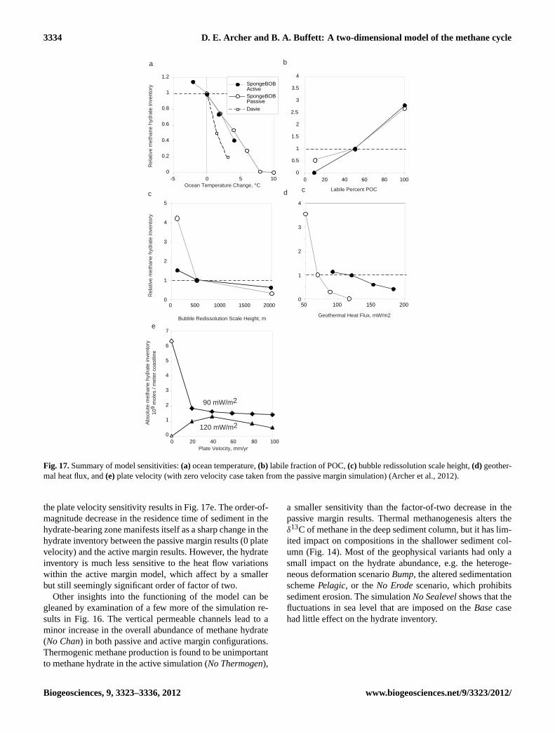
Figure 16 shows the hydrate inventories of all the simula-tions, and the results are digested into specific model sensi-tivities, and compared with results from the passive marginsimulation, in Fig. 17.

The sensitivity of the model to ocean temperature is sim-ilar between the passive and active models (Fig. 17a). Bothconfigurations of SpongeBOB are less temperature sensitive

Distance, km

δ13C DIC

0 40 80 120

Dep

th, k

m 2

4

6

0

-30

-10

10

0

-20

Fig. 15.Carbon isotopic composition,δ13C, of dissolved inorganiccarbon, for theBasescenario, with various other scenarios in theSupplement file del13dic.pdf. An animation ofδ13C of methane andDIC (Fig. 14) can be seen athttp://geosci.uchicago.edu/∼archer/spongebobactive/del13c.active.movie.gif.

than the Davie and Buffett (2001) model as deployed glob-ally by Buffett and Archer (2004).

Many of the other model sensitivities can be rationalizedas resulting from the differing sediment dynamics within thehydrate stability zone in the two model configurations. Theresidence time of sediment in the hydrate stability zone ismuch shorter in the active margin simulation, because sedi-ment flows horizontally through the wedge on a time scaleof only a few million years. In the passive margin setting, thelifetime of solid sediment in the stability zone is determinedby sediment accumulation, resulting in a residence time anorder of magnitude longer.

As a sediment parcel is carried laterally through thewedge, its depth below the sea floor increases as the sedi-ment column overall stretches in the vertical, carrying it forexample from shallow sediment depth in a deep water setting,within the hydrate stability zone, to relatively deeper depthsbelow the sea floor in the thicker sediment column in theshallower water onshore setting. The sediment is thus carriedthrough the same stages as a sediment parcel in the passivemargin configuration, from within the stability zone to belowthe zone, except on a horizontal pathway rather than verti-cal sediment accumulation. As the parcel crosses the hydratestability boundary, on either pathway, the methane solubil-ity reaches a maximum, then decreases as the parcel movesdeeper. The fluid tends to degas as the methane solubility de-creases below the stability boundary. The horizontal motionthus tends to act as an accumulator for methane, additionallyand operating more quickly than the analogous methane ac-cumulator from sedimentation and burial. At the same time,the shorter residence time for solid sediment in the hydrateaccumulation zone tends to limit the response of the steady-state hydrate inventory to many of the driving parameters.

The active margin configuration requires a higher min-imum availability of organic carbon (labile POC fraction

Biogeosciences, 9, 3323–3336, 2012 www.biogeosciences.net/9/3323/2012/

D. E. Archer and B. A. Buffett: A two-dimensional model of the methane cycle 3333

a

b

Met

hane

hyd

rate

inve

ntor

y10

9 m

oles

/ m

eter

coa

stlin

e

BaseBroadBumpFastplateSlowplate

2

0

4

Hyd

rate

mol

CH

4 . 1

09

0 5 10Model time, Myr

0

0.5

1

1.5

2

2.5

3

3.5

Base

Bio 10%

Bio 100%

T -2

T +

2

T +

4

No B

ubb Mig

Bubb 100m

Bubb 2km

Plate 100

Plate 80

Plate 20

Broad S

lope

Bum

p

No C

han

No E

rode

No T

hermoge n

Pelagic

Wide D

ef

No S

ealevel

Heat 90m

W

Heat 150m

W

Heat 180m

W

Pl 100 H

t 70

Pl 80 H

t 70

Pl 60 H

t 70

Pl 40 H

t 70

Pl 20 H

t 70

Fig. 16. (a)Time-dependent evolution of the scenarios showing variability due mostly to the coarse grid resolution.(b) Inventory of methanehydrate at the ends of the simulations for all model scenarios.

in these results) in order to cross the threshold to formingmethane hydrate (Fig. 17b). Presumably, the shorter lifetimeof sediment in the active margin stability zone requires some-what higher rate of methanogenesis in order to reach satura-tion in the shorter allotted time. This is the one example ofheightened sensitivity in the active margin configuration ofthe model.

The model sensitivity to the bubble redissolution scaleheight (Fig. 17c) is extremely muted in the active margin set-ting. Bubble redissolution as it migrates upward in the modelis a recycling mechanism, strengthening the efficiency of thehydrate stability zone as a cold trap. A more efficient coldtrap (shorter redissolution scale length) has a greater impactin the passive margin setting, because the sediment lifetimeis longer so the trap has more time to operate and accumulatehydrate.

The active configuration is also less sensitive to geother-mal heat flux (in Fig. 17d). Heat fluxes tend to be higherin active margin settings than passive, but the model results

show that the active margin configuration is more able to tol-erate higher heat fluxes than the passive configuration. In thepassive margin, a high geothermal heat flux creates a thin-ner stability zone, which in the fullness of time on the pas-sive margin allows the diffusive loss of methane sufficient todeplete the hydrate inventory. In the active margin, the ver-tical deformation tends to decrease the temperature gradientthrough the wedge, diminishing the impact of the basal heatflux on the near-surface temperature gradient and thicknessof the stability zone.

The model sensitivity to the plate velocity (Fig. 17e) ap-pears to be a convolution of several effects. Results are shownfrom two different values of the geothermal heat flux: onefrom the Basecase of the passive margin setting; and theother from the active margin. Recall from Fig. 17d that themodel is much more sensitive to the geothermal heat flux inthe passive margin, while the active margin appears to bufferthe hydrate inventory against depletion under conditions ofhigh geothermal heat flow. This same effect explains most of

www.biogeosciences.net/9/3323/2012/ Biogeosciences, 9, 3323–3336, 2012

3334 D. E. Archer and B. A. Buffett: A two-dimensional model of the methane cycle

Geothermal Heat Flux, mW/m2

Ocean Temperature Change, C

Rel

ativ

e m

etha

ne h

ydra

te in

vent

ory

0

0.2

0.4

0.6

0.8

1

1.2

-5 0 5 10

0

1

2

3

4

5

0 500 1000 1500 2000

Bubble Redissolution Scale Height, m

0

0.5

1

1.5

2

2.5

3

3.5

4

0 20 40 60 80 100

Labile Percent POC

Rel

ativ

e m

etha

ne h

ydra

te in

vent

ory

a b

c d

Davie

SpongeBOBPassive

SpongeBOBActive

0

1

2

3

4

c

50 100 150 200

Plate Velocity, mm/yr

0

1

2

3

4

5

6

7

0 20 40 60 80 100

Abs

olut

e m

etha

ne h

ydra

te in

vent

ory

109

mol

es /

met

er c

oast

line

e

120 mW/m2

90 mW/m2

Fig. 17.Summary of model sensitivities:(a) ocean temperature,(b) labile fraction of POC,(c) bubble redissolution scale height,(d) geother-mal heat flux, and(e)plate velocity (with zero velocity case taken from the passive margin simulation) (Archer et al., 2012).

the plate velocity sensitivity results in Fig. 17e. The order-of-magnitude decrease in the residence time of sediment in thehydrate-bearing zone manifests itself as a sharp change in thehydrate inventory between the passive margin results (0 platevelocity) and the active margin results. However, the hydrateinventory is much less sensitive to the heat flow variationswithin the active margin model, which affect by a smallerbut still seemingly significant order of factor of two.

Other insights into the functioning of the model can begleaned by examination of a few more of the simulation re-sults in Fig. 16. The vertical permeable channels lead to aminor increase in the overall abundance of methane hydrate(No Chan) in both passive and active margin configurations.Thermogenic methane production is found to be unimportantto methane hydrate in the active simulation (No Thermogen),

a smaller sensitivity than the factor-of-two decrease in thepassive margin results. Thermal methanogenesis alters theδ13C of methane in the deep sediment column, but it has lim-ited impact on compositions in the shallower sediment col-umn (Fig. 14). Most of the geophysical variants had only asmall impact on the hydrate abundance, e.g. the heteroge-neous deformation scenarioBump, the altered sedimentationschemePelagic, or theNo Erodescenario, which prohibitssediment erosion. The simulationNo Sealevelshows that thefluctuations in sea level that are imposed on theBasecasehad little effect on the hydrate inventory.

Biogeosciences, 9, 3323–3336, 2012 www.biogeosciences.net/9/3323/2012/

D. E. Archer and B. A. Buffett: A two-dimensional model of the methane cycle 3335

5 Conclusions

Active margin coastal settings tend to have high concentra-tions of methane hydrate in surface and near-surface sedi-ments, leading to a conceptualization of intense methane de-livery to surface sediments by pore fluid flow, driven by thedeformation of the thick sediment wedge. Previous models ofthe dynamics of methane in sediments were applied to activemargins by increasing the upward vertical pore fluid flow inthe model (Buffett and Archer, 2004; Chatterjee et al., 2011;Luff and Wallmann, 2003). An increase in upward flow leadsto an unambiguous increase in methane hydrate inventory inthis type of model.

The SpongeBOB model internalizes the pore fluid flow,predicting the flow rates from sediment accumulation, defor-mation, and pore pressure dynamics, rather than imposingthem as independent driving variables. As such it is diffi-cult to isolate the effect of pore fluid upward flow, becausethe rate of flow is driven largely by the rate of sediment col-umn convergence, which also changes other factors such asthe residence time of solid material in the hydrate-bearingzone. The model tends to produce higher pore-volume sat-urations (concentrations) of methane hydrate in the activemargin configuration than it does in the passive, but the ac-tive margin does not necessarily contain more hydrate permeter of coastline (total inventory) than the passive marginconfiguration. The horizontal transit of sediment through thehydrate-bearing zone appears to buffer the hydrate inventory,making it generally less sensitive to various driving param-eters such as the geothermal heat flux and the efficiency ofthe stability zone as a methane trap (the redissolution scaleheight parameter).

Supplementary material related to this article isavailable online at:http://www.biogeosciences.net/9/3323/2012/bg-9-3323-2012-supplement.zip.

Acknowledgements.This paper benefited from the commentsof the editor Jack Middelberg and reviewers Jerry Dickens andanother anonymous reviewer. The modeling project was funded byDOE NETL project DE-NT0006558. Plots were done using Ferret,a product of NOAA’s Pacific Marine Environmental Laboratory(http://ferret.pmel.noaa.gov/Ferret/).

Edited by: J. Middelburg

References

Archer, D. E., Buffett, B. A., and McGuire, P. C.: A two-dimensional model of the passive coastal margin deep sedimen-tary carbon and methane cycles, Biogeosciences, 9, 2859–2878,doi:10.5194/bg-9-2859-2012, 2012.

Batt, G. E., Brandon, M. T., Farley, K. A., and Roden-Tice, M.: Tec-tonic synthesis of the Olympic Mountains segment of the Casca-dia wedge, using two-dimensional thermal and kinematic model-ing of thermochronological ages, J. Geophys. Res.-Sol. Ea., 106,26731–26746, 2001.

Boswell, R. and Collett, T. S.: Current perspectives on gan hydrateresources, Energ. Environ. Sci., 4, 1206–1215, 2011.

Buffett, B. and Archer, D. E.: Global inventory of methane clathrate:Sensitivity to changes in environmental conditions, Earth Planet.Sci. Lett., 227, 185–199, 2004.

Carson, B., Suess, E., and Strasser, J. C.: Fluid-Flow and MassFlux Determinations at Vent Sites on the Cascadia Margin Ac-cretionary Prism, J. Geophys. Res.-Solid, 95, 8891–8897, 1990.

Chatterjee, S., Dickens, G. R., Bhatnagar, G., Chapman, W. G.,Dugan, B., Snyder, G. T., and Hirasaki, G. J.: Pore water sul-fate, alkalinity, and carbon isotope profiles in shallow sedi-ment above marine gas hydrate systems: A numerical mod-eling perspective, J. Geophys. Res.-Sol. Ea., 116, B09103,doi:10.1029/2011JB008290, 2011.

Davie, M. K. and Buffett, B. A.: A numerical model for the for-mation of gas hydrate below the seafloor, J. Geophys. Res., 106,497–514, 2001.

Davis, D., Suppe, J., and Dahlen, F. A.: Mechanics of fold-and-thrust belts and accretionary wedges, J. Geophys. Res., 88, 1153–1172, 1983.

Hunt, J. M.: Petroleum Geochemistry and Geology, Freeman, NewYork, 743 pp., 1995.

Hyndman, R. D. and Wang, K.: Thermal Constraints on the Zoneof Major Thrust Earthquake Failure – the Cascadia SubductionZone, J. Geophys. Res.-Sol. Ea., 98, 2039–2060, 1993.

Luff, R. and Wallmann, K.: Fluid flow, methane fluxes, carbonateprecipitation and biogeochemical turnover in gas hydrate-bearingsediments at Hydrate Ridge, Cascadia Margin: Numerical mod-eling and mass balances, Geochim. Cosmochim. Ac., 67, 3403–3421, 2003.

Malinverno, A., Kastner, M., Torres, M. E., and Wortmann, U. G.:Gas hydrate occurrence from pore water chlorinity and downholelogs in a transect across the northern Cascadia margin (IntegratedOcean Drilling Program Expedition 311), J. Geophys. Res.-Sol.Ea., 113, B08103,doi:10.1029/2008JB005702, 2008.

Mayer, L. M.: Surface area control of organic carbon accumulationin continental shelf sediments, Geochim. Cosmochim. Ac., 58,1271–1284, 1994.

Meiburg, E. and Kneller, B.: Turbidity currents and their deposits,Annu. Rev. Fluid Mech., 42, 135–156, 2010.

Milkov, A. V.: Global estimates of hydrate-bound gas in marine sed-iments: how much is really out there?, Earth-Sci. Rev., 66, 183–197, 2004.

Pohlman, J. W., Kaneko, M., Heuer, V. B., Coffin, R. B., andWhiticar, M.: Methane sources and production in the northernCascadia margin gas hydrate system, Earth Planet. Sci. Lett.,287, 504–512, 2009.

Spence, G. D., Hyndman, R. D., Chapman, N. R., Riedel, M.,Edwards, N., and Yuan, J.: Cascadia margin, northeast Pacific

www.biogeosciences.net/9/3323/2012/ Biogeosciences, 9, 3323–3336, 2012

3336 D. E. Archer and B. A. Buffett: A two-dimensional model of the methane cycle

Ocean: Hydrate distribution from geophysical investigations, in:Natural Gas Hydrate in Oceanic and Permafrost Environments,edited by: Max, M. D., Springer, 5, 183–198, 2000.

Torres, M. E., McManus, J., Hammond, D. E., de Angelis, M. A.,Heeschen, K. U., Colbert, S. L., Tryon, M. D., Brown, K. M., andSuess, E.: Fluid and chemical fluxes in and out of sediments host-ing methane hydrate deposits on Hydrate Ridge, OR, I: Hydro-logical provinces, Earth Planet. Sci. Lett., 201, 525–540, 2002.

Turcotte, D. L. and Schubert, G.: Geodynamics, Cambridge Univer-sity Press, Cambridge UK, 472 pp., 1982.

Wang, K., Hyndman, R. D., and Davis, E. E.: Thermal Effectsof Sediment Thickening and Fluid Expulsion in AccretionaryPrisms – Model and Parameter Analysis, J. Geophys. Res.-Sol.Ea., 98, 9975–9984, 1993.

Yuan, T., Spence, G. D., and Hyndman, R. D.: Seismic Velocitiesand Inferred Porosities in the Accretionary Wedge Sediments atthe Cascadia Margin, J. Geophys. Res.-Sol. Ea., 99, 4413–4427,1994.

Biogeosciences, 9, 3323–3336, 2012 www.biogeosciences.net/9/3323/2012/