a tutorial review of functional connectivity analysis

REVIEWpublished: 08 January 2016

doi: 10.3389/fnsys.2015.00175

Frontiers in Systems Neuroscience | www.frontiersin.org 1 January 2016 | Volume 9 | Article 175

Edited by:

Mikhail Lebedev,

Duke University, USA

Reviewed by:

Karim Jerbi,

University of Montreal, Canada

Mingzhou Ding,

University of Florida, USA

Craig Geoffrey Richter,

Ernst Strüngmann Institute, Germany

*Correspondence:

André M. Bastos

[email protected];

Jan-Mathijs Schoffelen

[email protected]

Received: 17 August 2015

Accepted: 30 November 2015

Published:

Citation:

Bastos AM and Schoffelen J-M (2016)

A Tutorial Review of Functional

Connectivity Analysis Methods and

Their Interpretational Pitfalls.

Front. Syst. Neurosci. 9:175.

doi: 10.3389/fnsys.2015.00175

A Tutorial Review of FunctionalConnectivity Analysis Methods andTheir Interpretational PitfallsAndré M. Bastos 1* and Jan-Mathijs Schoffelen 2, 3*

1Department of Brain and Cognitive Sciences, The Picower Institute for Learning and Memory, Massachusetts Institute of

Technology, Cambridge, MA, USA, 2Neurobiology of Language Department, Max Planck Institute for Psycholinguistics,

Nijmegen, Netherlands, 3Donders Centre for Cognitive Neuroimaging, Donders Institute for Brain, Cognition and Behaviour,

Radboud University Nijmegen, Nijmegen, Netherlands

Oscillatory neuronal activity may provide a mechanism for dynamic network coordination.

Rhythmic neuronal interactions can be quantified using multiple metrics, each with their

own advantages and disadvantages. This tutorial will review and summarize current

analysis methods used in the field of invasive and non-invasive electrophysiology to

study the dynamic connections between neuronal populations. First, we review metrics

for functional connectivity, including coherence, phase synchronization, phase-slope

index, and Granger causality, with the specific aim to provide an intuition for how these

metrics work, as well as their quantitative definition. Next, we highlight a number of

interpretational caveats and common pitfalls that can arise when performing functional

connectivity analysis, including the common reference problem, the signal to noise ratio

problem, the volume conduction problem, the common input problem, and the sample

size bias problem. These pitfalls will be illustrated by presenting a set of MATLAB-scripts,

which can be executed by the reader to simulate each of these potential problems. We

discuss how these issues can be addressed using current methods.

Keywords: functional connectivity (FC), coherence analysis, phase synchronization, granger causality,

electrophysiology, oscillations

INTRODUCTION

Different cognitive or perceptual tasks require a coordinated flow of information within networksof functionally specialized brain areas. It has been argued that neuronal oscillations provide amechanism underlying dynamic coordination in the brain (Singer, 1999; Varela et al., 2001; Fries,2005, 2015; Siegel et al., 2012). These oscillations likely reflect synchronized rhythmic excitabilityfluctuations of local neuronal ensembles (Buzsáki and Wang, 2012), and may facilitate the flowof neural information between nodes in the network when the oscillations are synchronizedbetween those nodes (Womelsdorf et al., 2007). The neural information transmitted from oneregion to another is reflected by the action potentials, where the action potentials themselvesmay be temporally organized in bursts. These bursts may occur during oscillations and mayfurther enhance the reliability of the information transmission (Lisman, 1997) or contribute tothe establishment of long-range synchronization (Wang, 2010). The brain could dynamicallycoordinate the flow of information by changing the strength, pattern, or the frequency with whichdifferent brain areas engage in oscillatory synchrony.

The hypothesis that neuronal oscillations in general, and inter-areal synchronization of theseoscillations in particular, are instrumental for normal brain function has resulted in widespread

08 January 2016

http://www.frontiersin.org/Systems_Neuroscience

http://www.frontiersin.org/Systems_Neuroscience/editorialboard




http://dx.doi.org/10.3389/fnsys.2015.00175

http://crossmark.crossref.org/dialog/?doi=10.3389/fnsys.2015.00175&domain=pdf&date_stamp=2016-01-08


http://www.frontiersin.org

http://www.frontiersin.org/Systems_Neuroscience/archive

https://creativecommons.org/licenses/by/4.0/

mailto:[email protected]

mailto:[email protected]

http://dx.doi.org/10.3389/fnsys.2015.00175

http://journal.frontiersin.org/article/10.3389/fnsys.2015.00175/abstract

http://loop.frontiersin.org/people/43260/overview

http://loop.frontiersin.org/people/269102/overview

Bastos and Schoffelen Functional Connectivity Analysis Tutorial

application of quantitative methods to evaluate neuronalsynchrony in electrophysiological data. These data can beobtained with invasive or non-invasive recording techniques,and in a context that involves an experimental manipulationor in a context that is task-free. Irrespective of the recordingtechnique and context, once the data have been collected theexperimental researcher is faced with the challenge to quantifyneuronal interactions as well as to provide a valid interpretationof the findings. We feel that this is challenging for severalreasons. First, the methods literature provides a multitude ofmetrics to quantify oscillatory interactions (for example, a recentreview characterized 42 distinct methods, Wang et al., 2014),often described with a large amount of technical detail. Somemethods, such as coherence and Granger causality, are basedon rigorous statistical theory of stochastic processes, whileothers, such as Phase-Locking Value (PLV) are modifications tothese methods that may be somewhat ad hoc, but neverthelessuseful. Each of these metrics has their own advantages anddisadvantages, and their own vigorous adherents and opponents.It is often difficult to choose and justify which method to use,even for the technically initiated. Second, since the algorithmicimplementation of a particular interaction metric can be quitecomplicated, some research groups may have an idiosyncraticimplementation of their championed interaction measures, withlimited accessibility to the wider research community. Thiscomplicates applicability of these particular metrics and thecomparison to other metrics. Third, the interpretation of thefindings is typically not straightforward and results are thereforeprone to being over-interpreted.

The purpose of this paper is to provide a (non-exhaustive)review and tutorial for the most widely used metrics to quantifyoscillatory interactions, and to provide the reader with anintuitive understanding of these metrics. First, we provide ageneral taxonomy of metrics to estimate functional connectivity.Next, we provide a more formal definition of the most commonlyused metrics, where possible illustrating the principles behindthese metrics using intuitive examples. In the last part, we discussvarious analysis pitfalls that one can encounter in applying thesemethods to real data. Using simulations, we generate synthetictime series to demonstrate how a multitude of practical issuescan arise to generate spurious functional connectivity, whichshould not be interpreted in terms of underlying neuronalinteractions. The different problems we discuss are signal-to-noise ratio (SNR) differences, limits in sample size, volumeconduction/electromagnetic field spread, the choice of reference,and the problem of unobserved inputs. The generation of thesynthetic time series as well as their analysis has been performedin MATLAB, using FieldTrip (Oostenveld et al., 2011), whichwill enable the comparison of how different data features affectthe metrics of oscillatory interactions, and how different metricsperform on the same data. For each simulation of commonpitfalls, where possible we present practical steps that can beused to mitigate the concerns. These simulations are put forwardas toy examples of some of the problems that can occur, andare not intended to reproduce the full complexity of real data.Yet, we hope that they will serve as a useful guide to commoninterpretation issues and the current state of the art in addressing

them. Finally, we also discuss where future methods might beuseful in order to deal with limitations of current methods.

TAXONOMY OF FUNCTIONALCONNECTIVITY METRICS

In this section, we will present a possible taxonomy of commonlyused metrics for functional connectivity (Figure 1) and brieflydescribe the main motivations for each of those methods.A first subdivision that can be made is based on whetherthe metric quantifies the direction of the interaction. Non-directed functional connectivity metrics seek to capture someform of interdependence between signals, without referenceto the direction of influence. In contrast, directed measuresseek to establish a statistical causation from the data that isbased on the maxim that causes precede their effects, andin the case of Granger causality and transfer entropy, thatcauses in some way predict their effects. These definitionsof statistical causality were originally developed by Wiener(1956) and later practically implemented using auto-regressivemodels by Granger (1969). In neuroscience, a rich and growingliterature has evolved that used these particular methodsto quantify neuronal interactions, which has been reviewedelsewhere (Bressler and Seth, 2011; Sakkalis, 2011; Seth et al.,2015).

Within both directed and non-directed types of estimates, adistinction can be made between model-free and model-basedapproaches. The model-based approaches depicted in Figure 1

FIGURE 1 | A taxonomy of popular methods for quantifying functional

connectivity.






all make an assumption of linearity with respect to the kindsof interactions that may take place between two signals. Thesimplest measure for non-directed model-based interactions isthe Pearson correlation coefficient, which measures the linearrelationship between two random variables. In the general linearmodeling framework the squared correlation coefficient (R2)represents the fraction of the variance of one of the variables (orsignals) that can be explained by the other, and vice versa. Amoregeneralized approach that does not assume a linear relationshipis mutual information (Kraskov et al., 2004), which measuresthe generalized (linear and non-linear) interdependence betweentwo or more variables (or time series) using concepts frominformation theory.

The Pearson correlation coefficient (and mutual information)as such are non-directed measures of interaction. Also, thesemeasures ignore the temporal structure in the data, and treatthe time series as realizations of random variables. In otherwords, this latter property means that the estimated connectivitywill be the same irrespective of whether the time series havebeen randomly shuffled or not. Yet, when we shift the twotime series with respect to one another before the correlationis computed (and do this shift at multiple lags), we will obtainthe cross-correlation function, and evaluation of the cross-correlation as a function of time lag does account for temporalstructure in the data. In particular, in some well-behaved cases itmay sometimes be used to infer directed neuronal interactions.Specifically, the cross-correlation function has been effectiveto study neuronal systems containing dominant unidirectionalinteractions that exert their largest influence at a specific timedelay (e.g., the retino-geniculate or geniculocortical feedforwardpathways, Alonso et al., 1996; Usrey et al., 1998). In thesecases, the time lag of maximal correlation and the magnitude ofcorrelation can be informative about information flow betweenbrain areas (e.g., Alonso et al., 1996). However, the interpretationof the cross-correlation function becomes complicated when it isestimated from neuronal signals with bidirectional interactions,which is the dominant interaction scenario in the majority ofcortico-cortical connections. The cross-correlation functions ofthese interactions typically lack a clear peak, and have significantvalues at both positive and negative lags, indicating complex,bi-directional interactions that occur at multiple delays.

To address this limitation, other methods can be used, whichassess the extent to which past values of one time series areable to predict future values of another time series, and viceversa. This notion is formally implemented in the metric ofGranger causality. This metric can be computed using a linearauto-regressive model fit to the data or through non-parametricspectral matrix factorization (described in more detail later), andallows for an estimation of directed interactions. In particular, itallows for a separate estimate of interaction from signal x to signaly, and from signal y to signal x.

Finally, model-free approaches have also been developed todetect directed interactions. For instance, transfer entropy isa generalized, information-theoretic approach to study delayed(directed) interactions between time series (Schreiber, 2000;Lindner et al., 2011). Transfer entropy is a more genericimplementation of the maxim that causes must precede and

predict their effects, and is able to detect non-linear forms ofinteraction, which may remain invisible to linear approacheslike Granger causality. In addition, transfer entropy has alsobeen extended to specifically measure directed interactionsbetween ongoing phase estimates of separate signals, which isuseful to study non-linear oscillatory synchronization (Lobieret al., 2014). However, due in part to its generality, it ismore difficult to interpret this measure. While the model-freeapproaches may be useful in quantifying non-linear neuronalinteractions, this review will focus on the model-based, linearmethods. Linear methods are sufficient to capture a wide-arrayof oscillatory interactions which are expected to take placeunder the hypothesis that oscillatory phase coupling governsneuronal interactions. For example, if we are interested indetermining whether neuronal oscillations at similar frequenciesin brain areas A and B engage in oscillatory coupling with apreferred phase difference, linear measures such as coherenceor PLV will capture this interaction. If on the other handwe are interested in non-linear forms of coupling, such ascross-frequency coupling (where the phase or amplitude offrequency f1 interacts with the phase or amplitude of frequencyf2, where f1 6= f2), then other metrics would be necessary.Therefore, the choice of method or data analysis shouldalways be guided by the underlying hypothesis that is beingtested.

A particularly important distinction if we wish to studyoscillations is the distinction between metrics that are computedfrom the time or frequency domain representation of the signals.In order to identify individual rhythmic components thatcompose the measured data, and specifically to study rhythmicneuronal interactions, it is often convenient to representthe signals in the frequency domain. The transformation tothe frequency domain can be achieved by the application ofnon-parametric (Fourier decomposition, wavelet analysis, orHilbert transformation after bandpass filtering) or parametrictechniques (autoregressive models). Subsequently, frequency-domain functional connectivity metrics can be estimatedto evaluate the neuronal interactions. As we will see, manyof these metrics in some way or another quantify theconsistency across observations of the phase differencebetween the oscillatory components in the signals. A non-random distribution of phase differences could be indicativeof functionally meaningful synchronization between neuralpopulations.

We also note that there are a diverse group of methodsthat operate purely on the amplitude (envelope) of theoscillations to quantify amplitude and power correlationsindependent of phase relations. These methods have beenfruitfully used to quantify large-scale brain networks by severalgroups (Hipp et al., 2012; Vidal et al., 2012; Foster et al.,2015). Indeed, there is now a growing debate about whetherphase-relations or amplitude relations govern large-scale brainnetworks, with evidence existing for both perspectives (seeFoster et al. this issue). In the following section we willfocus on frequency-domain metrics that require an estimateof the phase of the oscillations, as opposed to metrics thatquantify amplitude relations. Again, the choice of method






depends on the underlying hypothesis that is being tested. Phase-based methods are appropriate for testing hypotheses wherephase and moment-by-moment changes in synchronization areconsidered to be mechanisms for neuronal communication(e.g., Fries, 2005; Bastos et al., 2014). We will also not reviewmethods that quantify phase-amplitude coupling as they arebeyond the scope of this review and have been discussedextensively elsewhere (Canolty and Knight, 2010; Aru et al.,2015).

MEASURES OF SYNCHRONIZATION

In general measures of phase synchrony are computed fromthe frequency domain representation of a pair of signals,which represents across a set of observations (epochs or timewindows), and for a set of frequency bins, an estimate of theamplitude and the phase of the oscillations. Mathematically, it isconvenient to represent these amplitudes and phases combinedinto complex-valued numbers, Aeiϕ , or equivalently x + iy,which can be geometrically depicted as points in a 2-dimensionalCartesian coordinate system, where the magnitude of the vectorconnecting the point with the origin reflects the amplitude,and the angle of the vector with the X-axis reflects the phase(see Figure 2A; equivalently the x and y coordinates of thisnumber represent the Real and Imaginary parts, respectively).The spectral representation of individual signals is combinedto obtain the cross-spectral density (the frequency domainequivalent of the cross-covariance function), by means offrequency-wise multiplication of the spectral representation ofone of the signals with the complex conjugate of the spectralrepresentation of the other signal, where complex conjugationis defined as taking the negative of the phase angle. Thismultiplication results in a complex number, which geometricallydepicts a vector in 2-dimensional space, where the magnitudeof the vector reflects the product of the two signals’ amplitudes,and the angle between the vector and the X-axis reflects thetwo signals’ difference in phase (see Figure 2B). Measures ofphase synchrony now aim to capture some property of theprobability distribution of the single observation cross-spectraldensities, quantifying the consistency of the distribution of phasedifferences. One way to combine the cross-spectral densitieswould be to take a weighted sum, which geometrically amountsto drawing all vectors head to tail, and normalize the endresult. The idea is now that if there is some consistency acrossobservations of the phase difference between the two oscillatorysignals, the length of the weighted sum will have a non-zerovalue (because the vectors efficiently add up), whereas it will beclose to zero when the individual observations’ phase differencesare evenly distributed between 0 and 360◦. Figure 3 displaysthree “toy scenarios” to illustrate this concept. Imagine twooscillators that have a consistent zero-degree phase relation overmany trials or observation epochs. This is depicted graphicallyin the time domain in the left panels of Figure 3, showing twosignals (oscillation 1 and oscillation 2) that are observed forfour trials. The right panels of Figure 3 show the vector sumsof the cross-spectral densities. For the time being we assumedthe amplitude of the oscillations to have a value of 1. In the

first scenario (Figure 3A) the phase difference is the same (and0) for each of the observations, yielding a vector sum that hasa length of 4. In the second scenario, the phase difference isalso consistent across observations (i.e., 90◦ each time). In thethird scenario however, the phase difference is not consistentacross observations. In this example, the individual observations’phase differences were 0, 90, 180, and 270◦ respectively, resultingin individual observation cross-spectral density vectors pointingright, up, left and down. This results in a vector sum that has zerolength, which coincides with the fact that there was no consistentphase difference in this case. Note that real data will fall betweenthe two extremes of perfect phase synchronization (vector sumnormalized by number of epochs equals 1) and a zero phasesynchronization (vector sum to zero), even in the absence ofany true phase synchronization due to sample size bias (see thesection on sample size bias for an in depth discussion of this issueand how it can be mitigated).

The Coherence CoefficientOne widely used metric quantifying phase synchronybetween a pair of measured signals is the coherencecoefficient. Mathematically, the coherence is the frequencydomain equivalent to the time domain cross-correlationfunction. Its squared value quantifies, as a function offrequency, the amount of variance in one of the signalsthat can be explained by the other signal, or vice-versa,in analogy to the squared correlation coefficient in thetime domain. The coherence coefficient is a normalizedquantity bounded by 0 and 1, and is computed mathematicallyas:

cohxy(ω) =

∣

∣

∣

∣

1n

∑nk = 1 Ax(ω, k)Ay(ω, k)e

i(

ϕx(ω,k)−ϕy(ω,k))∣

∣

∣

∣

√

(

1n

∑nk=1 A

2x(ω, k)

)

(

1n

∑nk = 1 A

2y(ω, k)

)

(1)

The numerator term represents the length of the vectoraverage of the individual trial cross-spectral densities betweensignal x and y at frequency ω. The denominator representsthe square root of the product of the average of theindividual trial power estimates of signals x and y atfrequency ω.

It is usually more convenient to represent the averagedcross-spectral density in a single matrix, omitting the complexexponentials in the notation:

S (ω)=

[

Sxx (ω) Sxy (ω)

Syx (ω) Syy (ω)

]

The diagonal elements reflect the power estimates of signals xand y, and the off-diagonal elements reflect the averaged cross-spectral density terms. The coherence can then be conciselydefined as:

cohxy (ω)=

∣

∣Sxy(ω)∣

∣

√

Sxx(ω)Syy(ω)(2)






A B

FIGURE 2 | Using polar coordinates and complex numbers to represent signals in the frequency domain. (A) The phase and amplitude of two signals. (B)

The cross-spectrum between signal 1 and 2, which corresponds to multiplying the amplitudes of the two signals and subtracting their phases.

Coherency and the Slope of the PhaseDifference SpectrumWhen the magnitude operator (|. . . |) is omitted from thenumerator in equation above, we obtain a complex-valuedquantity called the coherency, where the phase difference anglemay be interpretable (if there is a clear clustering of phasedifference angles across trials) in terms of temporal delays. Thisis based on the notion that a consistent phase lag (or lead)across a range of frequency bins translates to a time lag (orlead) between the two time series. Note that the phase differenceestimate in a single frequency bin may be ambiguous in itsinterpretation, because a, say, −150◦ phase delay cannot bedisentangled from a +210◦ phase delay. This is due to the factthat the phase difference is circular modulo 360◦. However,observing the phase difference over a range of frequenciesmay give an unambiguous interpretation of temporal delays. Adisambiguated estimate of the time delay can be obtained whenthe rhythmic interaction can be described as a predominantlyunidirectional time-lagged linear interaction. This estimate isthen based on an estimate of the slope of the phase differenceas function of the frequency range in which there is substantialcoherence. This is because a fixed time delay between two timeseries leads to a phase difference that is a linear function offrequency. As an example, consider a time lag of 10ms anda rhythmic process with substantial oscillatory power in thefrequency range between 8 and 12Hz. At 8Hz, i.e., at a cycleduration of 125ms, a time shift of 10ms amounts 10/125 (0.08)of an oscillatory cycle (which amounts to 28.8◦). At 10Hz, thesame time shift amounts to 10/100 of an oscillatory cycle (36◦),and at 12Hz, a time shift of 10ms amounts to 10/83.33 (0.12)of an oscillatory cycle (43.2◦). We would like to emphasize,however, that an interpretation of the estimated slope of thephase difference spectrum in terms of a temporal delay (andthus as an indicator of directionality) is only valid under ratherideal circumstances, where the interaction is predominantlyunidirectional and well-captured under the assumption of

linearity. Under non-ideal circumstances, the phase differencespectrum is a complicated function of frequency, and using italone to assign directionality is un-principled (Witham et al.,2011; Friston et al., 2012).

Phase Slope IndexCompared to the slope of the phase difference spectrum,which assumes time-lagged and linear interactions, the phaseslope index (PSI) is a more generic quantity to inferdominant unidirectional interactions (Nolte et al., 2008). It iscomputed from the complex-valued coherency, and quantifiesthe consistency of the direction of the change in the phasedifference across frequencies. Given a pre-specified bandwidthparameter, it computes for each frequency bin the changein the phase difference between neighboring frequency bins,weighted with the coherence. As a consequence, if for a givenfrequency band surrounding a frequency bin the phase differencechanges consistently across frequencies, and there is substantialcoherence, the PSI will deviate from 0. The sign of the PSIinforms about which signal is temporally leading the other one.As discussed in the previous section, under situations whereinteractions are bi-directional, the phase difference spectrum(and consequently PSI) may fail at correctly describing thedirectionality. For further discussion of this, the reader is referredto Witham et al. (2011) and Vinck et al. (2015).

Imaginary Part of CoherencyWhen the complex-valued coherency is projected onto theimaginary axis (y-axis) we obtain the imaginary part of thecoherency (Nolte et al., 2004). This measure has gained somemomentum over the past years, in particular in EEG/MEGconnectivity studies (García Domínguez et al., 2013; Hohlefeldet al., 2013). Discarding contributions to the connectivityestimate along the real axis explicitly removes instantaneousinteractions that are potentially spurious due to field spread, asdiscussed in depth in a later section.






A

B

C

FIGURE 3 | The mechanics of the computation of phase synchrony. (A) An instance of perfect phase alignment at 0 radians. (B) An instance of perfect

synchronization at a difference of π/2 radians. (C) Absence of phase synchronization due to inconsistent phase differences.






Phase Locking ValueWhen applying the formula for the computation of coherence(Equation 1) to amplitude normalized Fourier transformedsignals, we get the phase locking value (PLV) (Lachaux et al.,1999):

plvxy (ω) =

∣

∣

∣

∣

1n

∑nk=1 1x(ω, k)1y(ω, k)e

i(


∣

∣

∣

√

(

1n

∑nk=1 1

2x(ω, k)

)

(

1n

∑nk=1 1

2y(ω, k)

)

=

∣

∣

∣

∣

1

n

∑n

k=1ei(


∣

∣

∣

As a result of these individual observation normalizations, thePLV is computed as the length of the vector-average of a set ofunit-length phase difference estimates. In motivating the use ofPLV, as opposed to coherence, it is often claimed that the formerreflects more strictly phase synchronization than coherence,because the latter confounds the consistency of phase differencewith amplitude correlation. From a mathematical point of viewthis may be true, but on the other hand one could argue that itis more “difficult” to obtain a meaningful non-zero coherencevalue in the absence of consistent phase differences, comparedto when there are no amplitude correlations. Intuitively, whenall individual observation cross-spectral density estimates arepointing in random directions (no phase synchrony), even inthe presence of perfect amplitude correlations, expected valueof their vector average will still be comparatively small. On theother hand, if all individual cross-spectral density estimates arepointing more or less into the same direction (strong phasesynchrony), even in the absence of amplitude correlations, theexpected value of their vector average will still be appreciable.Also, one could argue, in the case of coherence, that assigninga stronger weight to observations with a large amplitude product,one is favoring those observations that have a higher qualityphase difference estimate. This realistically assumes that a higheramplitude reflects a higher SNR of the sources of interest andthus, a better quality phase estimate.

Other Measures to Quantify ConsistentPhase DifferencesIn addition to the quantities described in the previous sections,over the past years various other metrics have been definedto quantify synchronized interactions between neuronal signals.The motivation for the development of these metrics is thatmost connectivitymetrics suffer from interpretational difficulties.These difficulties, which are discussed and illustrated in moredetail below, have prompted methods developers to definemetrics that are less prone to suffer from these problems.We havealready discussed the imaginary part of coherency and the phaseslope index, and this section describes two additional measuresthat are increasingly popular, the phase lag index (PLI), andpairwise phase consistency (PPC).

The PLI is a metric that evaluates the distribution of phasedifferences across observations. It is computed by averaging thesign of the per observation estimated phase difference (Stam et al.,

2007). It is motivated by the fact that non-zero phase differencescannot be caused by field spread (just like with the imaginarypart of coherency and the PSI). More recently, some adjustmentsto the PLI have been proposed, yielding the weighted PLI anddebiased weighted PLI to make the metric more robust againstfield spread, noise and sample-size bias (Vinck et al., 2011).

The PPC is a measure that quantifies the distribution ofphase differences across observations (Vinck et al., 2010). Unlikethe PLV, which is computed directly as a vector average of therelative phase across observations, the PPC is computed fromthe distribution of all pairwise differences (between pairs ofobservations) of the relative phases. The idea behind this is that,similar to the situation when investigating the distribution ofrelative phases directly, the distribution of pairwise differencesin the relative phases will be more strongly clustered around anaverage value in the presence of phase synchronization. Whenno phase synchronization is present, the individual relative phasevectors are distributed around the unit circle, as are all pairwisedifferences of these relative phase vectors. The advantage of PPCbeyond PLV is that this metric is not biased by the sample sizethat is used for the estimation. This means that the expected valueof PPC does not change as a function of trial number (see sectiontitled “The sample size bias problem” for more details).

In essence, many of the measures mentioned as such are notbased on a principled mathematical approach (as opposed to forinstance coherence and Granger causality which are rooted in thetheory of stochastic processes). For instance PLI, the imaginarypart of the coherency, and the phase slope index are pragmaticmeasures primarily put forward to address the interpretationalproblem of field spread, and by design intend to capture similarfeatures of the interaction between time series. It is often anempirical question as to which of the measures is most suitedto be used, and ideally one should expect that the conclusionsdrawn do not strongly depend on the measure that was chosen.Therefore, in general it is advisable to interrogate the data usingseveral of these measures, in order to get a feel for how theestimates relate to one another.

Going Beyond Pairwise InteractionsSo far we have discussed connectivity metrics that are definedbetween pairs of signals. Often, however, more than two signalshave been recorded, and it may be relevant to investigate inmore detail the pattern of multiple pairwise interactions. Forthis, graph theoretic approaches can be employed (Sporns,2011). These approaches build on a valid quantification of theconnectivity, are discussed extensively elsewhere and are beyondthe scope of this tutorial. It is brought up here as a prelude to thenext section, where we discuss the problem of common input.In general, the problem at stake is the correct inference of adirect interaction in the presence of other (possibly unobserved)sources. Although latent, unobserved sources pose a fundamentaland irresolvable problem, information from sources that havebeen observed can be used to remove indirect influences on theestimation of connectivity. One of the ways in which this canbe done in the context of coherence analysis, is by means ofusing the partial coherence (Rosenberg et al., 1998). If multiplesignals have been recorded, one can compute for any signal






pair the so-called partialized cross-spectrum, which is obtainedby removing the linear contribution from all the other signals.From the partialized cross-spectrum, the partial coherence can beeasily obtained. The partialized cross-spectrum can be obtainedas follows. Starting from the full cross-spectral density matrix,

S (ω)=

Sxx (ω) Sxy (ω) Sxz1 (ω) . . . Sxzn (ω)

Syx (ω) Syy (ω) Syz1 (ω) . . . Syzn (ω)

Sz1x (ω) Sz1y (ω) Sz1z1 (ω) . . . Sz1zn (ω)

......

.... . .

...Sznx (ω) Szny (ω) Sznz1 (ω) . . . Sznzn (ω)

we can partialize for the linear contributions from signals z1-znto the cross spectrum between signal x and y as follows:

S\z (ω) =

[

Sxx(ω) Sxy (ω)

Syx(ω) Syy (ω)

]

−

[

Sxz1 (ω) . . . Sxzn (ω)

Syz1 (ω) . . . Syzn (ω)

]

Sz1z1 (ω) . . . Sz1zn (ω)

.... . .

...Sznz1 (ω) . . . Sznzn (ω)

−1

Sz1x (ω) Sz1y (ω)

......

Sznx (ω) Szny (ω)

=

[

Sxx\z (ω) Sxy\z (ω)

Syx\z (ω) Syy\z (ω)

]

Spike-Field CoherenceWith invasive electrophysiological signals, it is possible torecord action potentials from single neurons and/or clustersof neurons (sometimes referred to as multiunit activity). Inthis situation, it can be informative to examine how ongoingoscillations in the simultaneously recorded LFP or EEG arerelated to the spikes. To this end, spikes from a given unitcan be represented as a time series of ones and zeros, at thesame sampling rate as the continuous LFP/EEG signals (notethat it is possible to represent the spikes as a vector of spiketimes—this can sometimes lead to a sparser representationof the data). Once a suitable representation of the spikes ischosen, we can compute any of the above-mentioned metricsof synchronization between spikes and fields, and indeed alsobetween different spike trains. This can often reveal significantmodulation of spike timing relative to field oscillations (e.g.,significant spike-field coherence), which can also be sensitiveto task variables (e.g., Fries et al., 2001; Gregoriou et al.,2009). Spike-field analysis comes with its own host of caveatsand challenges, which are beyond the scope of this review(interested readers can refer to Vinck et al., 2012; Ray,2015).

QUANTIFICATION OF FREQUENCYRESOLVED, DIRECTED INTERACTIONSWITH GRANGER CAUSALITY

So far, we have reviewed connectivity metrics that at best inferdirectionality of interactions based on the sign of the phasedifference of the band-limited oscillatory signal components. Yet,the practical applicability of these techniques is limited to cases

where there is a consistently time-lagged and predominantly uni-directional interaction. Granger causality and related metrics arecapable of quantifying bi-directional interactions and providestwo estimates of directed connectivity for a given signal pair,quantifying separately the directed influence of signal x on signaly, and the directed influence of signal y on signal x. Originally,the concept of Granger causality was applied to time seriesdata in the field of economics (Granger, 1969), and extensionof the concept to the frequency domain representation of timeseries was formulated by Geweke (1982). Although excellentintroductory texts exist that explain the concept of frequencydomain Granger causality and their application to neurosciencedata (Ding et al., 2006), we briefly review the essential conceptsin some detail in the Appendix (Supplementary Material). At thispoint, we restrict ourselves to the necessary essentials.

Time Domain FormulationIn essence, Granger causality represents the result of a modelcomparison. It is rooted in the autoregressive (AR) modelingframework, where future values of time series are modeled as aweighted combination of past values of time series. Specifically,the quality of an AR-model can be quantified by the varianceof the model’s residuals, and Granger causality is defined as thenatural logarithm of a ratio of residual variances, obtained fromtwo different AR-models. One of these models reflect a univariateAR-model, where values of time series x are predicted as aweighted combination of past values of time series x. The othermodel is a bivariate AR-model, where the values of time series xare predicted not only based on past values of x, but also based onpast values of another time series y.A substantial reduction of thevariance of the residuals comparing the univariate model to thebivariate model implies that the inclusion of information aboutthe past values of signal y in the prediction of signal x (aboveand beyond inclusion of only past values of signal x) leads to abetter model for time series x. In these cases, the variance ratiois larger than 1, which leads to a Granger causality value that islarger than 0, signal y is said to Granger cause signal x (Granger,1969; Ding et al., 2006; Bressler and Seth, 2011). Applying thesame logic but now building autoregressive models to predictsignal y will yield an estimate of Granger causality from signalx to y.

Frequency Domain FormulationThe concept of Granger causality can also be operationalizedin the frequency domain (Geweke, 1982). We refer theinterested reader to the Appendix (Supplementary Materialand the references mentioned therein) for more details.Here, it is sufficient to state that computation of Grangercausality in the frequency domain requires the estimation oftwo quantities: the spectral transfer matrix (H(ω)), which isfrequency dependent, and the covariance of the AR-model’sresiduals (6). The following fundamental identity holds:H(ω)6H(ω)∗ = S(ω), with S(ω) being the cross-spectraldensity matrix for signal pair x, y at frequency ω. In otherwords, the conjugate-symmetric cross-spectral density can beobtained by sandwiching the covariance matrix of the residualsbetween the spectral transfer matrix. From the cross-spectrum,






the spectral transfer matrix and the residuals’ covariance matrix,the frequency-dependent Granger causality can be computed asfollows:

GCx→y(ω) = ln

Syy(ω)

Syy (ω)−(6xx −62yx

6yy)∣

∣Hyx(ω)∣

∣

2

Relationship Between Frequency DomainGranger Causality and CoherenceJust as in the time domain formulation of Granger causality, it ispossible to define a measure of total interdependence, based onthe cross-spectral density estimates [more details are provided inthe Appendix (Supplementary Material)]:

GCx,y(ω) = − ln

(

1−

∣

∣Sxy(ω)∣

∣

2

Sxx (ω) Syy (ω)

)

The fraction between the brackets is equivalent to the squaredcoherence coefficient, as shown in an earlier section. Inother words, there is a one-to-one relationship between thecoherence coefficient and the total interdependence. In analogyto the time domain formulation, the frequency specific totalinterdependence can be written as a sum of three quantities:GCx,y(ω) = GCx→y(ω) + GCy→x(ω) + GCx·y(ω), where theinstantaneous causality term is defined as:

GCx·y(ω) =

ln

(

Syy(ω)−(6xx−62yx

6yy)∣

∣Hyx(ω)∣

∣

2)(

Sxx (ω)−(6yy−62xy

6xx)∣

∣Hxy(ω)∣

∣

2)

det(S (ω))

This latter term reflects the part of the total interdependencethat cannot be accounted for by time-lagged (phase-shifted)interactions between signals x and y, reflecting instantaneouscommon input from latent sources. Note that in the case of zero-phase lag synchronization the instantaneous causality term is notnecessarily larger relative to the causal terms. Specifically, in asystem with bidirectional interactions, where the magnitude andphase delay of the transfer function are approximately equal inboth directions (i.e., from x to y, and from y to x), the cross-spectral densitymatrix can report strong synchronization at zero-phase delay that is nonetheless brought about by strong time-delayed causal interactions in both directions. Note, however,that theoretical work points out that zero-lag phase coupling ismuch more likely to occur in the presence of a dynamic relaythrough a third source, which gives common input to stabilizephase relations across the network at zero-lag (Vicente et al.,2008). Practically, this situation can be distinguished from apurely bi-directional interaction only if the two nodes with zero-lag synchronization were observed simultaneously with the thirdnode that may (or may not) provide common inputs. Moredetails on this scenario and how to detect it in physiological dataare provided in the section “The common input problem.”

Non-Parametric vs. ParametricComputation of Granger CausalityGranger causality in the frequency domain can be calculated withparametric methods (with auto-regressive models, as discussed,left half of Figure 4) or with non-parametric methods (withFourier or wavelet-based methods). These approaches differ inhow the covariance of the residuals and the transfer matrices arecomputed (see the right half of Figure 4). The non-parametricapproach is based on the fact that the cross-spectral densitymatrix for a given frequency is equal to the model’s residualscovariance matrix sandwiched between the transfer matrix forthat frequency, as outlined above:

S(ω) = H(ω)6H∗(ω).

Starting from the cross-spectral density matrix (and thus goinginto the opposite direction) it is possible to factorize the cross-spectral density matrix into a “noise” covariance matrix andspectral transfer matrix by applying spectral matrix factorization(Wilson, 1972)—which provides the necessary ingredients forcalculating Granger causality (see Equation 4, Dhamala et al.,2008). It has been shown that parametric and non-parametricestimation of Granger causality yield very comparable results,particularly in well-behaved simulated data (Dhamala et al.,2008).

The main advantage in calculating Granger causality usingthis non-parametric technique is that it does not require thedetermination of the model order for the autoregressive model.The particular choice of the appropriate model order canbe problematic, because it can vary depending on subject,experimental task, quality and complexity of the data, andmodel estimation technique that is used (Kaminski and Liang,2005; Barnett and Seth, 2011). In contrast, the non-parametricestimation of Granger causality utilizes data points from the

FIGURE 4 | Data processing pipeline for the computation of Granger

causality, using the parametric or non-parametric approach.






entire frequency axis, the number of which is essentiallydetermined by the number of samples in the data window thatis used for the analysis.

In comparison to the parametric estimation technique, thenon-parametric spectral factorization approach requires moredata and a smooth shape of the cross-spectral density (i.e.,no sharp peaks as a function of frequency) to converge to astable result. This can be seen most acutely when attemptingto compute Granger causality from single trials. Although bothparametric and non-parametric techniques can be used forsingle-trial estimates of directed connectivity, it appears thatparametric estimates are more sensitive than non-parametricestimates, especially when the model order is known (Brovelli,2012; Richter et al., 2015).

Bivariate vs. Multivariate SpectralDecompositionIt is relevant to note that, in multichannel recordings, the spectraltransfer matrix can be obtained in two ways, irrespective ofwhether it is computed from a fitted autoregressive model,or through factorization of a non-parametric spectral densityestimate. One can either fit a full multivariate model (orequivalently, do a multivariate spectral decomposition), whereall channels are taken into account, or one can do the analysisfor each channel pair separately. The latter approach typicallyyields more stable results (e.g., because it involves the fitting offewer parameters), but the advantage of the former approach isthat information from all channels is taken into account whenestimating the interaction terms between any pair of sources.In this way, one could try and distinguish direct from indirectinteractions, using an extended formulation of Granger causality,called partial Granger causality (Guo et al., 2008), or conditionalGranger causality (Ding et al., 2006; Wen et al., 2013). Also,the multivariate approach yields a spectral transfer matrix thatcan be used to compute a set of connectivity metrics, whichare related to Granger causality. These metrics are the directedtransfer function (DTF) with its related metrics (Kamiñski andBlinowska, 1991), and partial directed coherence (PDC) with itsrelated metrics (Baccalá and Sameshima, 2001). These quantitiesare normalized between 0 and 1, where the normalization factoris either defined as the sum along the rows of the spectral transfermatrix (for DTF), or as the sum along the columns of the inverseof the spectral transfer matrix (for PDC). By consequence of thesenormalizations, DTF from signal y to x reflects causal inflow fromy to x as a ratio of the total inflow into signal x, while in its originalformulation PDC from signal y to signal x reflects the causaloutflow from y to x as a ratio of the total outflow from signal y.These measures, and their derivatives, along with motivations forpreferring one over the other metric, are discussed in more detailin for example (Blinowska, 2011).

LIMITATIONS AND COMMON PROBLEMSOF FUNCTIONAL CONNECTIVITYMETHODS

The following section outlines some issues that warrant cautionwith respect to the interpretation of the estimated connectivity.

The core issue at stake is whether the estimate of the connectivity(or the estimate of the difference in connectivity betweenexperimental conditions) reflects a genuine effect in terms of(a change in) neuronal interactions. As we will illustrate bymeans of simple simulations, there are various situations thatcause non-zero estimates of connectivity in the absence of trueneuronal interactions. Themain cause of these spurious estimatesof connectivity is the fact that in MEG/EEG/LFP recordingsthe signals that are used for the connectivity estimate always tosome extent reflect a (sometimes poorly) known mixture of asignal-of-interest (which is the activity of a neuronal populationthat we are interested in) and signals-of-no-interest (which wewill call noise in the remainder of this paper). Another causeof spurious estimates is more related to interpretation of theobserved connectivity patterns. This relates to the fact that it isimpossible to state whether an observed connection is a directconnection, or whether this connection is mediated through anunobserved connection.

In what follows, we describe five common practical issues thatwarrant caution with respect to the interpretation of connectivityestimates. We illustrate these problems using simple simulationsthat are based on MATLAB-code and the FieldTrip toolbox,allowing the interested reader to get some hands-on insightinto these important issues. The code has been tested onMATLAB 2013a/b and 2014a/b, using Fieldtrip version “fieldtrip-20150816.” The first three problems (the common referenceproblem, the volume conduction/field spread problem, and theSNR problem) are a consequence of the fact that the measuredsignals are always a mixture of signal-of-interest and noise, andthe 4th is the problem of unobserved common input. The 5thproblem is caused by unequal numbers of epochs or observationperiods used to compute metrics of functional connectivity whenmaking comparisons between conditions or across subjects.

THE COMMON REFERENCE PROBLEM

In LFP or EEG recordings, spurious functional connectivityestimates can result from the usage of a common referencechannel. This problem is depicted graphically in Figure 5A.Imagine two recorded time series, data 1 and data 2. Eachof these signals reflects the difference of the electric potentialmeasured at the location of the electrode and at the locationof the reference electrode. If the same reference electrodeis used for both electrodes that are subsequently used forthe connectivity estimation, the fluctuations in the electricpotential at the reference location will be reflected in bothtime series, yielding spurious correlations at a zero time lag.Any connectivity metric that is sensitive to correlations at azero time lag will in part be spurious. The extent to whichthe estimated connectivity is spurious depends on the relativestrength of the potential fluctuations at the recording andreference sites. Obviously, the large majority of EEG and LFPrecordings use a single reference electrode in the hardware. Thefollowing simulation illustrates the effect of a common referenceelectrode. We will simulate 30–60Hz oscillatory activity intwo neuronal sources, and this activity is measured by twoelectrodes that share a common reference electrode (whichis also assumed to have an oscillatory component). We will






A B C

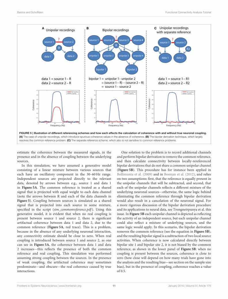
FIGURE 5 | Illustration of different referencing schemes and how each effects the calculation of coherence with and without true neuronal coupling.

(A) The case of unipolar recordings, which introduce spurious coherence values in the absence of coherence. (B) The bipolar derivation technique, which largely

resolves the common reference problem. (C) The separate reference scheme, which also is not sensitive to common reference problems.

estimate the coherence between the measured signals, in thepresence and in the absence of coupling between the underlyingsources.

In this simulation, we have assumed a generative modelconsisting of a linear mixture between various sources thateach have an oscillatory component in the 30–60Hz range.Independent sources are projected directly to the relevantdata, denoted by arrows between e.g., source 1 and data 1in Figure 5A. The common reference is treated as a sharedsignal that is projected with equal weight to each data channel(note the arrows between R and each of the data channels inFigure 5). Coupling between sources is simulated as a sharedsignal that is projected into each source in some mixture,specified in the script (sim_commonreference.pdf ). Using thisgenerative model, it is evident that when no real coupling ispresent between source 1 and source 2, there is significantartifactual coherence between data 1 and data 2, due to thecommon reference (Figure 5A, red trace). This is a problem,because in the absence of any underlying neuronal interaction,any connectivity estimate should be close to zero. When realcoupling is introduced between source 1 and source 2, as onecan see in Figure 5A, the coherence between data 1 and data2 increases—this reflects the presence of both the commonreference and real coupling. This simulation was performedassuming strong coupling between the sources. In the presenceof weak coupling, the artifactual coherence may sometimespredominate—and obscure—the real coherence caused by trueinteractions.

One solution to the problem is to record additional channelsand perform bipolar derivation to remove the common reference,and then calculate connectivity between locally-rereferencedbipolar derivations that do not share a common unipolar channel(Figure 5B). This procedure has for instance been applied inBollimunta et al. (2009) and in Bosman et al. (2012), and relieson two assumptions: first, that the reference is equally present inthe unipolar channels that will be subtracted, and second, thateach of the unipolar channels reflects a different mixture of theunderlying neuronal sources—otherwise, the same logic behindeliminating the common reference through bipolar derivationwould also result in a cancelation of the neuronal signal. Fora more rigorous discussion of the bipolar derivation procedureand its applications to neural data, see Trongnetrpunya et al. thisissue. In Figure 5B each unipolar channel is depicted as reflectingthe activity of an independent source, but each unipolar channelcould also reflect a mixture of underlying sources, and thesame logic would apply. In this scenario, the bipolar derivationremoves the common reference (see the equation in Figure 5B),and the resulting bipolar signal is a subtraction of two local sourceactivities. When coherence is now calculated directly betweenbipolar site 1 and bipolar site 2, it is not biased by the commonreference, as shown in the lower panel of Figure 5B: when nocoupling is present between the sources, coherence is close tozero (how close will depend on how many trials have gone intothe analysis and the resulting bias—see section on the sample sizebias), but in the presence of coupling, coherence reaches a valueof 0.5.






A second possible solution to this problem is shown inFigure 5C, which is to separately reference each channel.In this case (lower panel of Figure 5C), there is again noartifactual coherence component. Therefore, while the separatereferencing scheme does present a solution in principle, itmay not be practical for large-scale, high density recordings.The simulations above can be realized by running the code inscript sim_commonreference.pdf. Note that in these simulations,the reference was also assumed to have an oscillatory 30–60Hz component—however, if the reference consisted of whitenoise, or a mixture of white and colored noise, and coherencewere calculated between channels which both had a commonreference, then the respective coherence spectrum would reflectwhatever the underlying spectral shape of the reference was—dueto its instantaneous mixture into both channels.

THE VOLUME CONDUCTION/FIELDSPREAD PROBLEM

Another important issue in the quantification and interpretationof neuronal interactions, particularly when the estimatesare based on non-invasive recordings, is caused by volumeconduction. Strictly speaking, volume conduction refers to thecurrents flowing in the tissues surrounding active neuronalsources. Colloquially it has been adopted as a term to reflectmore generally the phenomenon of the spatial spread ofelectromagnetic fields, which cause one recording channel orsensor to pick up the activity of multiple neuronal sources.In the case of magnetic field recordings it is sometimes moreaptly referred to as field spread. At its worst, field spread cancreate purely artifactual coherence or phase-locking, meaningthat the presence of functional connectivity between two signalswould indicate not the presence of a true neuronal interaction,but instead the presence of activity from the same underlyingsource at the two channels. An important property of volumeconduction and field spread, at least in the frequency range thatis relevant for neuroscience, is that its effects are instantaneous.That is, if a dominant rhythmic neuronal source is visible at twosensors at once, the phase observed at these sensors is the same(or at a difference of 180◦, when each of the sensors “sees” anopposite pole of the dipole). This property of instantaneity can beexploited to use connectivity measures that discard contributionsof 0 (or 180) degrees phase differences. This will be explained inmore detail below.

When considering the different electrophysiological recordingtechniques, field spread is considered the least problematic ininvasive recordings. Spiking activity of individual neurons is bydefinition very focal spatially, and volume currents associatedwith this spiking can only be picked up at a distance of a fewtens or hundreds of microns. Therefore, for the quantificationof spike-spike or spike-field interactions, field (Kajikawa andSchroeder, 2011) spread is hardly an issue. In the interpretationof synchronization estimated between two LFP signals, volumeconduction needs to be taken into account. The reason is thatthe local field potentials may reflect volume currents propagatingover larger distances, exceeding 1 cm (Kajikawa and Schroeder,

2011). Field spread is by far the most problematic whenperforming non-invasive measurements, because of the largedistance between the sensors and the neural sources, and becauseof the spatial blurring effect of the skull on the electric potentialdistribution on the scalp with EEG (Nunez et al., 1997, 1999;Srinivasan et al., 2007; Winter et al., 2007; Schoffelen and Gross,2009). By consequence, a single underlying neuronal source willbe seen at multiple EEG or MEG sensors—causing spuriouscorrelation values between the sensors.

In the presence of field spread any given source is “visible”on multiple sensors/electrodes at once, and several strategiesmay be employed to alleviate the adverse effects of field spread.The first strategy attempts to “unmix” the measured signals toderive an estimate of the underlying sources. In the context ofEEG/MEG recordings one should think of the application ofsource reconstruction algorithms (Schoffelen and Gross, 2009).In the context of LFP recordings one should think of theapplication of a re-referencing scheme, using for example alocal bipolar derivation (as reviewed in the previous section),or estimating the current source density. The second strategyrelates to the use of well-controlled experimental contrasts.The assumption here is that volume conduction affects theconnectivity estimates in a similar way in both conditions, andsubtraction will effectively get rid of the spurious estimates.A third strategy, as already mentioned above, would be touse connectivity metrics that capitalize on the out-of-phaseinteraction, discarding the interactions that are at a phasedifference of 0 (or 180◦). Examples of these metrics are theimaginary part of the coherency, the (weighted) phase lag index,or the phase slope index. At the expense of not being able todetect true interactions occurring at near zero-phase difference,these metrics at least provide an account of true (phase-lagged)interactions between signal components. Unfortunately, neitherthe application of source reconstruction techniques (whichmoreover add a level of complexity to the analysis of the data),nor the use of experimental contrasts or phase-lagged interactionmeasures will fully mitigate the effects of volume conduction.This has been described in more detail elsewhere (Schoffelen andGross, 2009).

The script sim_volumeconduction.pdf illustrates some of theissues mentioned above, as well as the approaches that partiallyovercome them. The general approach in this set of simulationsis that a set of signals is simulated at 50 “measurement locations”(MEG/EEG channels, or at “virtual electrodes”). Each of thesignals consists of a mixture (due to field spread) of the activityof the underlying sources. The source activity time coursesare generated by means of a generative autoregressive model.The source-to-signal mixing matrix was defined as a spatialconvolution of the original source activations with a 31-pointHanning window. In other words we can consider the signals toconsist of a weighted combination of the original source and the15 most nearby sources on either side, with a spatial leakage thatis dependent on the distance.

Figure 6A shows connectivity matrices for all sensor pairs,and the source signals were constructed such that none ofthe underlying sources were interacting (i.e., there were nocross-terms in the autoregressive model coefficients). The noise






A C

D

B

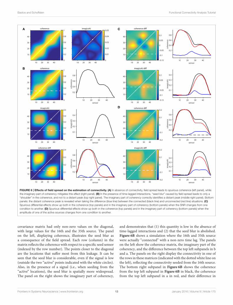
FIGURE 6 | Effects of field spread on the estimation of connectivity. (A) In absence of connectivity, field spread leads to spurious coherence (left panel), while

the imaginary part of coherency mitigates this effect (right panel). (B) In the presence of time-lagged interactions, “seed blur” caused by field spread leads to only a

“shoulder” in the coherence, and not to a distant peak (top right panel). The imaginary part of coherency correctly identifies a distant peak (middle right panel). Bottom

panels: the distant coherence peak is revealed when taking the difference (blue line) between the connected (black line) and unconnected (red line) situations. (C)

Spurious differential effects show up both in the coherence (top panels) and in the imaginary part of coherency (bottom panels) when the SNR changes from one

condition to another. (D) Spurious differential effects show up both in the coherence (top panels) and in the imaginary part of coherency (bottom panels) when the

amplitude of one of the active sources changes from one condition to another.

covariance matrix had only non-zero values on the diagonal,with large values for the 16th and the 35th source. The panelon the left, displaying coherence, illustrates the seed blur asa consequence of the field spread. Each row (column) in thematrix reflects the coherence with respect to a specific seed sensor(indexed by the row number). The points closer to the diagonalare the locations that suffer most from this leakage. It can beseen that the seed blur is considerable, even if the signal is low(outside the two “active” points indicated with the white circles).Also, in the presence of a signal (i.e., when seeding from the“active” locations), the seed blur is spatially more widespread.The panel on the right shows the imaginary part of coherency,

and demonstrates that (1) this quantity is low in the absence oftime-lagged interactions and (2) that the seed blur is abolished.Figure 6B shows a simulation where the 16th and 35th sourcewere actually “connected” with a non-zero time lag. The panelson the left show the coherence matrix, the imaginary part of thecoherency, and the difference between the top left subpanels in band a. The panels on the right display the connectivity in one ofthe rows in thesematrices (indicated with the dotted white line onthe left), reflecting the connectivity seeded from the 16th source.The bottom right subpanel in Figure 6B shows the coherencefrom the top left subpanel in Figure 6B in black, the coherencefrom the top left subpanel in a in red, and their difference in






blue. So far, these simulations demonstrate in a very simplifiedscenario the effects of field spread, as well as the remedial effectsprovided by subtracting two conditions with different levels ofconnectivity between the active sources, or by focusing on thetime-lagged component of the connectivity.

Real experimental data, however, is hardly ever as well-behaved as the simulated data presented above. The followingprovides some non-exhaustive examples of cases where theremedial strategies may yield results that can be wronglyinterpreted. Figure 6C shows a situation where a true connectionexists between the 16th and the 35th source, which doesn’tchange in strength from one condition to another. In one ofthe conditions an additional source is active (at location 27),which is not connected to any of the other sources. The differencemaps, however, show quite some spatial structure, which isdue to the differential effects exerted by the field spread onthe connectivity estimates. For example, seeding from the 11thsource using coherence as a connectivity metric yields a spuriousnon-zero difference around the 25th source. This is shown inthe right panel of Figure 6C, where the individual conditions’seed-based connectivity estimates are displayed as red and blacklines, and their difference is displayed in blue. Likewise, seedingfrom the 22nd source using the imaginary part of coherencyyields a spurious non-zero difference around the 28th source.The implication of this is that differences in the activity in thecontributing sources can yield spurious differences in estimatedconnectivity. One could argue that an appropriate seed selectionwould have prevented this erroneous interpretation. Had wefocused on the active sources to begin with, the problemmay havebeen less severe. Although there may be some truth in this, inpractice it is often difficult to select the proper seeds a priori, forexample because the relevant sources are not necessarily the onesthat have the highest amplitude, and even if the seed locationsare appropriately selected, spurious connectivity can stillarise.

This is illustrated in Figure 6D, where two conditions arecompared, with unchanging connectivity between the activatedsources (16 and 35), but with a change in power for one ofthem. The panels on the right show the seeded connectivity(from source 16) for the condition with low (red lines) and high(black lines) power for source 35, as well as their difference (bluelines).

The difficulty of interpreting connectivity estimates due tofield spread, as described above, can also be problematic fora correct inference of directed connectivity, e.g., by means ofGranger causality, or related quantities. The reason for this is thatthe linearmixing of the source signals due to the field spread leadsto signal to noise ratio differences between channels (discussedmore in the next section), and inaccuracies in the estimation ofthe spectral transfer matrix and the noise covariance. Althoughsome simulation work indicates that the true underlying networkconnectivity may be recovered by applying a renormalizedversion of PDC (Elsegai et al., 2015), Vinck et al. (2015)showed that instantaneous mixing is problematic for an accuratereconstruction of Granger causality. These authors propose touse a heuristic based on the investigation of the instantaneousinteraction between signals in relation to their time-delayed

interactions, in order to discard or accept the estimated directedconnectivity to be trustworthy.

THE SIGNAL-TO-NOISE RATIO PROBLEM

Another issue that leads to interpretational problems of estimatedconnectivity is what we call here the SNR problem. In some waythis problem is related to the field spread problem discussedabove, since its underlying cause is the fact that the measuredsignals contain a poorly known mixture of signal-of-interest,and “noise.” Some consequences of this have already beenillustrated to some extent above, where the comparison betweenconditions leads to spurious differences in connectivity, dueto differences in SNR across conditions. Apart from posinga problem for correctly inferring a difference in connectivityacross conditions, SNR differences can also be problematic wheninferring differences in directional interactions between sources.It should be noted that this problem can also arise in the absenceof volume conduction (e.g., when computing connectivity fromlocally-rereferenced LFP recordings), and therefore we believethat this problem merits a separate discussion. The core issuehere is that spurious directional connectivity estimates can beobtained from two signals that have each been observed withdifferent amounts of signal and noise. Such a situation canfor instance arise when across LFP recording sites there aredifferences in sensor noise (e.g., due to differences in amplifiercharacteristics), or differences in distance to the active sourcesof interest, causing a difference in signal strength. While this isa problematic issue for many metrics of directed connectivity,in this section we focus specifically on how estimates ofGranger causality can be corrupted by differences in SNRbetween signals. We illustrate the issue by presenting somesimulations, which can be realized by running the code in scriptsim_signaltonoise.pdf.

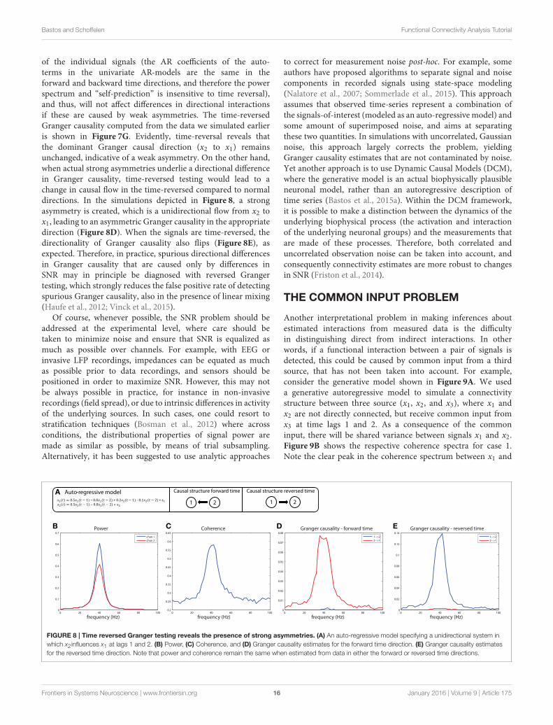
To understand why differences in SNR are likely to beproblematic for the estimation of Granger causality, it isuseful to remember that one variable has a Granger causalinfluence to another if the past of one time series can enhancepredictions about another. In general, this approach will workto detect true connectivity, however, when applied to noisydata, this definition of causality based on prediction can leadto unexpected consequences. Imagine a situation shown inFigure 7A: variables x1and x2 are generated by an auto-regressiveprocess that is a function of their own past at time lags 1and 2 (the auto terms), and also a function of the past ofthe other variable (the cross terms), also at time lag 1 and2. Crucially, the auto-regressive coefficients of both the auto-terms and the cross terms are identical, and the variance ofthe innovations (ε1, ε2) of both processes are also identical,meaning that the two variables influence each other with equalstrength. Therefore, by construction, Granger causality fromx1 to x2 should be identical compared to Granger causalityfrom x2 to x1. This is indeed the case when the outputs ofsuch a generative process are observed without measurementnoise, illustrated in Figures 7B–D. In this case, as expected, bothvariables have nearly identical power spectra peaking at 40Hz






A

B C D

E F G

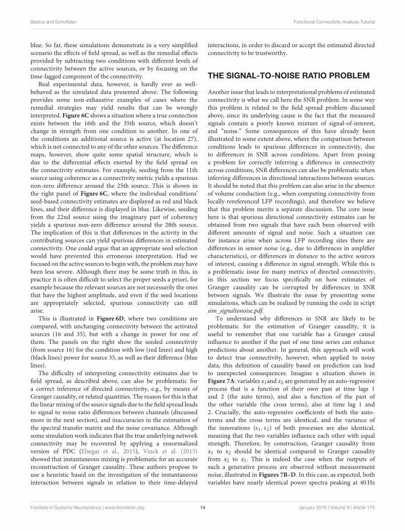
FIGURE 7 | A simulation of the signal to noise ratio problem. (A) Two nodes interact bidirectionally with equal connectivity strengths in the two directions, and

the data is observed without (case 1) or with (case 2) measurement noise. (B) Power for case 1, (C) Coherence for case 1 and 2, and (D) Granger causality estimates

for case 1. (E) Power, (F) Granger causality estimates for case 2. (G) Granger causality estimates after time-reversing the data produced by case 2.

(Figure 7B), have a coherence spectrum that also peaks at 40Hz(Figure 7C), and have approximately equal Granger causalityat 40Hz in both directions (Figure 7D). Note that the slightdifference in Granger causality from x1 to x2 vs. x2 to x1 isdue to estimation error, which approaches zero as the numberof realizations of the model and subsequent observations arerepeated.

Now let us consider case 2, where we observe the same system,but in the presence of noisy measurements. In this case, whitenoise is added to x1, but not to x2. The first result of thismanipulation is that the power spectrum of x1 is shifted upward(Figure 7E), a result of adding power at all frequencies (i.e., whitenoise) to that channel. The coherence between the channels isalso modulated by this manipulation, shown in Figure 7C, with areduction in coherence at a broad range of frequencies when extranoise is present. When looking at the Granger causal estimates,shown in Figure 7F, we observe an asymmetric relationship,where x2 has a stronger Granger causal influence on x1 than x1 onx2. This is the consequence of the fact that the additional noise onx1 has weakened its predictive power of x2, causing an apparentasymmetry in the directionality. Note that this asymmetry is

exactly in line with the definition of Granger causality based ona log ratio of prediction errors (comparing the univariate to thebivariate model), and in that sense it is not “wrong.” However,this does lead to a divergence between “Granger causality” andwhat we as experimentalists would like to infer as “true causality,”where we would like to infer a dominant direction of informationflow from an asymmetry in Granger causal estimates.

These simulations depict the “worst case scenario,” when amassive difference in SNR exists between channels (SNR of x1was 1, SNR of x2 was maximal because there was no noiseadded). Asymmetries in Granger causality that are driven bySNR differences have been defined by Haufe et al. as “weakasymmetries,” as opposed to “strong asymmetries” caused bytrue time-lagged, causal relationships (Haufe et al., 2012). Inorder to be able to make a distinction between weak and strongasymmetries in the interpretation of the estimated Grangercausality, Haufe et al. suggest to investigate Granger causalityafter time-reversal of the signals. The underlying rationaleis that time-reversal causes a flip in the dominant directionof interaction only in the presence of strong asymmetries,because the time-reversal operation does not affect the SNR






of the individual signals (the AR coefficients of the auto-terms in the univariate AR-models are the same in theforward and backward time directions, and therefore the powerspectrum and “self-prediction” is insensitive to time reversal),and thus, will not affect differences in directional interactionsif these are caused by weak asymmetries. The time-reversedGranger causality computed from the data we simulated earlieris shown in Figure 7G. Evidently, time-reversal reveals thatthe dominant Granger causal direction (x2 to x1) remainsunchanged, indicative of a weak asymmetry. On the other hand,when actual strong asymmetries underlie a directional differencein Granger causality, time-reversed testing would lead to achange in causal flow in the time-reversed compared to normaldirections. In the simulations depicted in Figure 8, a strongasymmetry is created, which is a unidirectional flow from x2 tox1, leading to an asymmetric Granger causality in the appropriatedirection (Figure 8D). When the signals are time-reversed, thedirectionality of Granger causality also flips (Figure 8E), asexpected. Therefore, in practice, spurious directional differencesin Granger causality that are caused only by differences inSNR may in principle be diagnosed with reversed Grangertesting, which strongly reduces the false positive rate of detectingspurious Granger causality, also in the presence of linear mixing(Haufe et al., 2012; Vinck et al., 2015).

Of course, whenever possible, the SNR problem should beaddressed at the experimental level, where care should betaken to minimize noise and ensure that SNR is equalized asmuch as possible over channels. For example, with EEG orinvasive LFP recordings, impedances can be equated as muchas possible prior to data recordings, and sensors should bepositioned in order to maximize SNR. However, this may notbe always possible in practice, for instance in non-invasiverecordings (field spread), or due to intrinsic differences in activityof the underlying sources. In such cases, one could resort tostratification techniques (Bosman et al., 2012) where acrossconditions, the distributional properties of signal power aremade as similar as possible, by means of trial subsampling.Alternatively, it has been suggested to use analytic approaches

to correct for measurement noise post-hoc. For example, someauthors have proposed algorithms to separate signal and noisecomponents in recorded signals using state-space modeling(Nalatore et al., 2007; Sommerlade et al., 2015). This approachassumes that observed time-series represent a combination ofthe signals-of-interest (modeled as an auto-regressive model) andsome amount of superimposed noise, and aims at separatingthese two quantities. In simulations with uncorrelated, Gaussiannoise, this approach largely corrects the problem, yieldingGranger causality estimates that are not contaminated by noise.Yet another approach is to use Dynamic Causal Models (DCM),where the generative model is an actual biophysically plausibleneuronal model, rather than an autoregressive description oftime series (Bastos et al., 2015a). Within the DCM framework,it is possible to make a distinction between the dynamics of theunderlying biophysical process (the activation and interactionof the underlying neuronal groups) and the measurements thatare made of these processes. Therefore, both correlated anduncorrelated observation noise can be taken into account, andconsequently connectivity estimates are more robust to changesin SNR (Friston et al., 2014).

THE COMMON INPUT PROBLEM

Another interpretational problem in making inferences aboutestimated interactions from measured data is the difficultyin distinguishing direct from indirect interactions. In otherwords, if a functional interaction between a pair of signals isdetected, this could be caused by common input from a thirdsource, that has not been taken into account. For example,consider the generative model shown in Figure 9A. We useda generative autoregressive model to simulate a connectivitystructure between three source (x1, x2, and x3), where x1 andx2 are not directly connected, but receive common input fromx3 at time lags 1 and 2. As a consequence of the commoninput, there will be shared variance between signals x1 and x2.Figure 9B shows the respective coherence spectra for case 1.Note the clear peak in the coherence spectrum between x1 and

A

B C D E

FIGURE 8 | Time reversed Granger testing reveals the presence of strong asymmetries. (A) An auto-regressive model specifying a unidirectional system in

which x2 influences x1 at lags 1 and 2. (B) Power, (C) Coherence, and (D) Granger causality estimates for the forward time direction. (E) Granger causality estimates

for the reversed time direction. Note that power and coherence remain the same when estimated from data in either the forward or reversed time directions.






1

3

2

– + - +

– +

Generative model

B

0 20 40 60 80 1000

0.1

0.2

0.3

0.4

0.5

0.6

0.7

1−>2

2−>1

3−>1

3−>2

1−>3

2−>3

1

3

2

– + +

– +

Generative model

t = 1

t = 2

0 20 40 60 80 1000

0.005

0.01

0.015

0.02

0.025

0.03

0.035

0.04

0.045

0.05

1−>2

2−>1

A

t = 1 & 2

t = 1 & 2

Granger causality - case 1Coherence - case 1

Case 2 - !me-lagged common input

(only nodes 1 and 2 observed)

Case 1 - !me-lagged common input

(all nodes observed)



frequency (Hz) frequency (Hz)


C

ED F

1−2

1−2 imaginary

1−3

2−3

G Case 3 - !me-lagged common input

(all nodes are observed)

1

3

2

– + +

– +

Generative model

t = 1

t = 2

0 20 40 60 80 1000

0.1

0.2

0.3

0.4

0.5

0.6

0.7


H I

1−2

1−2 | 3

1−3

2−3

0 20 40 60 80 1000

0.1

0.2

0.3

0.4

0.5

0.6

0.7

0.8

0 20 40 60 80 1000

0.05

0.1

0.15

0.2

0.25

0.3

0.35

1−2

1−2 imaginary

1−>2

2−>1

3−>1

3−>2

1−>3

2−>3

0 20 40 60 80 1000

0.1

0.2

0.3

0.4

0.5

0.6

0.7

0.8

1−2 | 3

FIGURE 9 | A simulation of the common input problem. (A) The auto-regressive form of a model that simulates common input from x3 to x1 and x2. (B) spurious

coherence between x1 and x2 caused by common input. Imaginary coherence (green) and partial coherence (purple) are close to zero, indicating an interaction that is

both instantaneous and mediated (by x3), respectively. (C) Granger causal estimates detect the common input as distinct from directed interactions between x1 and

x2 (which are near zero). (D–F) When time-lagged common input from x3 is present and only x1 and x2 are observed, the data will appear to reflect a time-lagged

interaction. This situation can only be interpreted correctly by recording the common driver (G,H), and applying partial coherence (H) or multivariate Granger

causality (I).

x2 at 40Hz (blue trace). If we were to interpret this coherencespectrum as evidence of a direct neuronal interaction, it wouldbe a spurious inference. Therefore, to aid in the interpretation ofthis coherence spectrum, we need to explicitly consider whetherthe shared variance that causes the observed coherence is due tocommon input. If we observe all three nodes, this can be doneby considering coherence between x1and x2 after partializingout the contribution of x3(magenta trace in Figure 9B), whichreports substantially reduced coherence values between x1andx2, indicative of shared variance (coherence) due to commoninput. Another metric to look at in this case would be theimaginary part of coherency (green trace), which is also close

to zero, indicating that shared variance between x1 and x2can be accounted for entirely by the zero-lag component, ascould be expected by field spread or, in this case, by commoninput that arrives simultaneously and at the same lags at x1andx2.

We can also examine whether the shared variance betweenx1and x2 is due to effects of their direct interaction or commoninput by computing Granger causality. Figure 9C shows theGranger causality estimates between x1, x2, and x3 based ona multivariate decomposition of the spectral density matrix,i.e., observing all three nodes. By decomposing the undirectedconnectivity into directed connectivity using Granger causality,






only connections with true underlying coupling (connectionsx3 x1 and x3 x2) survive, and the spurious connections(x1 x2 and x2 x1) are suppressed, because the shared varianceis absorbed by their instantaneous interactions which are not partof a causal (lagged) interaction. This would also be a situationwhere conditional or partial Granger causality would be usefulfor diagnosing the true underlying connectivity between x1, x2,and x3. These simulations can be realized by running the code inscript sim_commoninput.pdf.

Note that we have assumed that the common input is providedwith equal coupling strength, at the same time delay, and thatrecordings are performed with an equal signal to noise ratio.In real data, as these assumptions are progressively violated, theestimates of Granger causality will also start to reflect spuriousdirectional coupling. This is because changes in any of theseparameters will affect how well the variance in one node canpredict variance in other nodes and therefore change Grangercausality values, as demonstrated in the section on signal tonoise ratio. This can be especially problematic if one has notrecorded from the node providing common input. This situationis simulated in the next example (case 2, Figure 9D), where x3provides time-lagged common input by influencing x1 at lag 1and x2 at lag 2. Coherence and Granger causality, computed afterobserving only x1and x2 are shown in Figures 9E,F. Coherenceshows a strong coupling, which is phase-delayed due to the timelag offset in the common drive (the imaginary part of coherency,the green trace, reports almost identical values as ordinarycoherence). This situation results in a significantly asymmetricGranger causality metric, with the x1 x2 influence dominantover the x2 x1influence (case 3, Figure 9G). In this particularexample, the only way to correctly infer the true connectivitystructure would be to observe all three nodes and performmultivariate Granger causality (Figures 9G–I). Figure 9H showsthat there exists strong coherence between all three nodes, eventhough the coherence between x1and x2 is a result of (time-lagged) common input. This can again be detected by performingpartial coherence (Figure 9H, magenta trace) which removesthe linear contribution of x3 onto the coherence between x1and x2 (driving it close to zero). Furthermore, multivariate

Granger causality (Figure 9I) correctly decomposes the truecausal structure.

For networks with more than three nodes, there has beensome progress toward inferring true network causality even inthe presence of unobserved time-lagged common inputs. Inparticular, Elsegai and colleagues develop a technique based onrenormalized PDC together with sub-network analysis, althoughthe method can only resolve the correct connectivity in asubset of possible interactions (Elsegai et al., 2015). Therefore,common inputs can still lead to spurious inference, and currentlythe only guaranteed way to overcome this problem is bydirectly measuring nodes that could putatively provide commoninput.

THE SAMPLE SIZE BIAS PROBLEM

Sample size bias can be a problem when connectivity measuresare being compared between two or more conditions where thenumber of observations used to compute connectivity is differentbetween the conditions. In general, measures of connectivity(with a few exceptions, such as PPC) are often biased quantities,where under the null hypothesis of no connectivity the estimateswill deviate from zero. One of the reasons for this is that manyof these metrics reflect the magnitude of a vector quantity,which always has a positive value, which is just a different wayof stating that the expected value will never be zero (exceptin highly contrived scenarios such as Figure 3C). The amountof bias is often dependent on the sample size: the smaller thesample size, the larger the bias. The consequence of this isthat, in the comparison of connectivity metrics estimated fromsamples with different numbers of observations, there may be atendency to overestimate the connectivity in the condition withthe smallest sample size. Also, more importantly, even in theabsence of true interactions, non-zero difference may be foundand reported.

In order to obtain estimates of phase synchronization usingnon-parametric spectral estimation techniques, a necessary stepis to take a vector summation operation which is then normalizedby the total number of trials. When fewer trials are used to

A B C

FIGURE 10 | Sample size bias for coherence and Granger causality estimates. (A–C) For each respective metric, simulations based on 5, 10, 50, 100, and

500 trials were run, and coherence (A), Granger causality (B), and PPC (C) were calculated. Each panel reflects the average ± 1 standard deviation across 100

realizations.






estimate the phase consistency, even in the absence of phasesynchrony, these vectors can all align in the same directionmore easily (thereby summing to a non-zero coherence value)compared to when many trials are used. This bias is shownin Figure 10A (derived from the script sim_samplesizebias.pdf ),where 100 simulations of a simple auto-regressive model wererealized, after calculating coherence based on 5, 10, 50, 100, and500 trials. Estimating coherence based on lower trial numbersyields an average coherence value, which is substantially higherand also more variable over different estimates compared withhigher trial counts. Figure 10B shows the same simulationbut using Granger causality as connectivity measure. Thisshows that measures like coherence, PLV, and Granger causalityare positively biased when estimated using non-parametrictechniques, and this fact should be taken into account for aproper inference. To estimate how much bias is present in agiven estimate, one can create a reference distribution by re-arranging data segments and destroying the temporal alignmentbetween channels. This would preserve the power spectrum ofeach signal but should force the cross terms of the cross spectrumto approach zero. After repeating the procedure of temporalre-alignment and connectivity estimation, one can comparethe empirically observed connectivity estimate to the referencedistribution and determine an appropriate level of significance.To estimate the absolute value of a connectivity metric likeGranger causality, one can subtract the estimated bias to obtaina de-biased estimate (Barnett and Seth, 2014). Note that thisapproach is only successful in eliminating the sample-size biasassociated with connectivity estimates. Other phenomena thatinflate the connectivity estimates such as field spread are notproperly taken into account by trial-shuffling procedures andmust be dealt with in other ways.

Several approaches can be taken to account for the samplesize bias. In some experimental situations, where the number ofobservations per condition is more or less balanced by design(but in practice turns out to be different, e.g., after artifactrejection), one strategy could be to equate the number oftrials across conditions to be compared by randomly deletingobservations from the condition with higher trial numbers untilthe trial numbers are equated. This approach is ideally embeddedin a bootstrap procedure, where the random deletion of trialsis repeated multiple times, to obtain a more robust estimate.In addition, for some metrics (for instance for coherence)analytic estimates of the bias can be computed and applied(Bokil et al., 2007). For coherence this usually goes hand inhand with a variance stabilizing Z-transform, which has theadded advantage to facilitate a meaningful group statisticalinference. Another possibility is to account for the differentsample size bias within the inferential statistical framework,using a non-parametric statistical test (Maris et al., 2007).Or, in the specific case of coherence, one can consider thedistributional properties and do parametric statistical inferenceusing a jackknife procedure (Bokil et al., 2007). Alternatively,one could use a metric for detecting synchronization whichis inherently unbiased, such as PPC (see Figure 10C). Finally,one could also estimate the bias associated with any particularmeasure of functional connectivity (for example, by shuffling the

trial sequence of one channel relative to others, and calculatingthe metric of functional connectivity), and then subtract awaythis estimate of bias from the empirically observed connectivityvalue.

CONCLUSION

In this paper, we have presented a non-exhaustive review ofdifferent methods currently used to quantify rhythmic functionalconnectivity. We described a taxonomy to emphasize how themethods are related to one another. For some of the mostcommonly used metrics, we also described the intuition behindthem and some of the mathematical formulation. This was meantto demystify what data features are reflected in these connectivitymetrics and how they are computed. Next we presented someimportant issues that may confound a correct interpretation ofthe connectivity, estimated from electrophysiological recordings.The description of these issues was accompanied by a series ofsimple simulations.

We hope that these simulations have impressed upon thereader that a naïve application of connectivity analysis toobserved electrophysiological time series data can result in amyriad of spurious inferences. The simulations presented inthis manuscript were meant to illustrate some of the mostcommon cases where interpretational difficulties await theeager experimental scientist. These include problems associatedwith use of a common reference, the presence of volumeconduction/field spread, differences in signal to noise ratio,observed or unobserved common inputs, and bias related todifferences in sample size. In addition, by making available theMATLAB scripts that were used to perform the simulations,we hope that readers are encouraged run these simulationsthemselves, and that they will not shy away from changingthe parameters in the scripts to explore in more detail theramifications of these potential interpretational confounds. Also,the scripts can be used as a controlled environment wheredifferent solutions to these confounds can be developed andexplored before they are applied on real data.

Where possible, we illustrated potential solutions to theinterpretational pitfalls that we have explored. For the commonreference problem, we discussed how local referencing via bipolarderivation or current source density estimation can be effectiveat removing common signal components. Another possibleapproach is to use a metric which explicitly discards the zerolag component of the interaction. Next, we discussed how thevolume conduction/field spread problem can be approachedin three distinct ways: by source reconstruction or local re-referencing, via the use of experimental contrasts (which makesthe sometimes invalid assumption that volume conduction effectsare constant between conditions), or by using methods that areinsensitive to volume conduction such as the imaginary partof coherency. Field spread also affects the estimates of directedfunctional connectivity. Currently, there is no guaranteedmethod to discard volume conduction effects in this case. Oneway to protect against false positive inferences is to investigatethe instantaneous interaction to determine whether field spread






effects are too large to warrant an analysis (Vinck et al., 2015).Another possibility in principle is to include volume conductionwithin the estimation framework of Granger causality, whichwould require further development of model-based approachesto connectivity estimation.

The problem of a different signal to noise ratio across channelswas discussed in the light of the potential misinterpretation ofthe dominant direction of interaction using directed connectivityestimates, in particular Granger causality. We illustrated a testbased on time-reversed Granger causality (Haufe et al., 2012)to determine whether Granger causal asymmetries are due tostrong vs. weak asymmetries in the data. In addition, we pointedout novel approaches that are based on state-space modelingand DCM, which explicitly consider the separate contribution ofsignal and noise to the estimated connectivity.

The problem of common input was also discussed, whichis particularly relevant when researchers want to make claimswith respect to whether the interaction between two neuronalgroups is direct, or mediated by a third source. In general itis impossible to distinguish direct from indirect interactionsif not all nodes of the functionally connected network aresampled. The problem is not a theoretical one. For instance, thereis increasing evidence that some cortico-cortical interactionsare mediated by the thalamus (Sherman and Guillery, 2011).Using LFP recordings from the thalamus and two cortical areas(V4 and TEO) Saalmann and colleagues showed that alpha-band cortico-cortical coherence between V4 and TEO wasalmost entirely eliminated after conditioning on the thalamicdrive (Saalmann et al., 2012). The problem of commoninput can be theoretically dealt with by actually recordingfrom the nodes that potentially provide common input, andby calculating a multivariate decomposition and conditionalGranger causality or partial coherence. In practice this solutionmay not always be feasible due to limitations in the experimentalset up. Yet, over the past years much progress has beenmade in increasing the coverage of neuroscience methods.For example, single cell resolution and close to full brainsampling can now be accomplished in the neonatal zebrafish,using Calcium imaging (Ahrens et al., 2013). In addition,methods that allow for significant brain coverage and densespatial sampling of LFP and spiking activity are now becomingincreasingly available in both animals (Rubehn et al., 2009;Salazar et al., 2012; Berényi et al., 2014; Schwarz et al., 2014;Lewis et al., 2015) as well as human patients undergoingneurosurgical treatments (Chang, 2015; Khodagholy et al.,2015).

Finally, we discussed the effect of sample size bias inconnectivity estimates. This problem can be dealt with byequalizing sample sizes between conditions or subjects, by usingstatistical methods that explicitly take the sample size bias intoaccount, or by using connectivity methods which do not sufferfrom sample size bias (PPC or debiased methods).

These simulations were implemented using the FieldtripToolbox (Oostenveld et al., 2011). We note that other

toolboxes are also available for estimation of functionalconnectivity data, most notably EEGLAB and the SIFTtoolbox (Delorme et al., 2011), the MVGC toolbox (Barnettand Seth, 2014), the Hermes toolbox (Niso et al., 2013),the TRENTOOL toolbox (Lindner et al., 2011) for transferentropy calculation, and the Chronux toolbox (Mitra andBokil, 2008). Many of these tools are open source, and benefitfrom a wide community of users and contributors, whichhelp to improve the tools and contribute to a larger-scaleadoption.

We end by emphasizing that the difficulties we have noteddo not preclude a meaningful analysis of connectivity inelectrophysiological data, even when some of these issues arepresent. One relevant aspect that briefly needs to be mentionedis that the appropriate use of an inferential statistical procedureis a crucial step in the application of connectivity estimationtechniques to neuroscience data, and in the correct interpretationof the results. Statistical tests are used to both establishsignificance of connectivity (against the null hypothesis of nosignificant coupling) as well as to establish significant changesin coupling between conditions (against the null hypothesis ofno significant changes). This is typically done within a non-parametric statistical testing framework (Maris et al., 2007)and/or using bootstrap sampling and trial-reshuffling (seeMethods Section in Bastos et al., 2015b). Yet, a statisticalprocedure used inappropriately may still lead to an over-interpretation of results (e.g., inferring significant coherencewhen it is actually artifactual or inferring a difference ininteraction in the presence of differences in signal to noise ratioacross conditions). We hope that the explicit discussion of theinterpretational issues described in this review raises awarenessin the wider neuroscientific community. At the same time, newmethods are being continuously developed to address theseproblems. Overall, one can be optimistic for the future as betterdata, more nuanced hypotheses and experiments, and improvedanalysis tools continue to provide new insights into the brain’sdynamic connectivity.

ACKNOWLEDGMENTS

This research was in part funded by an NWO VIDI-grant(864.14.011) to JS. AMB was partly funded by the NationalScience Foundation Graduate Student Fellowship Program anda Fulbright grant from the U.S. Department of State. The authorswould like to thank Alik Widge for providing comments to anearlier version of this manuscript, and to the three reviewerswhose comments have improved the paper.

SUPPLEMENTARY MATERIAL

The Supplementary Material for this article can be foundonline at: http://journal.frontiersin.org/article/10.3389/fnsys.2015.00175


http://journal.frontiersin.org/article/10.3389/fnsys.2015.00175





REFERENCES

Ahrens,M. B., Orger, M. B., Robson, D. N., Li, J. M., and Keller, P. J. (2013).Whole-

brain functional imaging at cellular resolution using light-sheet microscopy.

Nat. Methods 10, 413–420. doi: 10.1038/nmeth.2434

Alonso, J. M., Usrey, W. M., and Reid, R. C. (1996). Precisely correlated

firing in cells of the lateral geniculate nucleus. Nature 383, 815–819. doi:

10.1038/383815a0

Aru, J., Aru, J., Priesemann, V., Wibral, M., Lana, L., Pipa, G., et al. (2015).

Untangling cross-frequency coupling in neuroscience. Curr. Opin. Neurobiol.

31, 51–61. doi: 10.1016/j.conb.2014.08.002

Baccalá, L. A., and Sameshima, K. (2001). Partial directed coherence: a new

concept in neural structure determination. Biol. Cybern. 84, 463–474. doi:

10.1007/PL00007990

Barnett, L., and Seth, A. K. (2011). Behaviour of Granger causality under filtering:

theoretical invariance and practical application. J. Neurosci. Methods 201,

404–419. doi: 10.1016/j.jneumeth.2011.08.010

Barnett, L., and Seth, A. K. (2014). The MVGC multivariate Granger causality

toolbox: a new approach to Granger-causal inference. J. Neurosci. Methods 223,

50–68. doi: 10.1016/j.jneumeth.2013.10.018

Bastos, A. M., Litvak, V., Moran, R., Bosman, C. A., Fries, P., and Friston, K. J.

(2015a). A DCM study of spectral asymmetries in feedforward and feedback

connections between visual areas V1 and V4 in the monkey. Neuroimage 108,

460–475. doi: 10.1016/j.neuroimage.2014.12.081

Bastos, A. M., Vezoli, J., Bosman, C. A., Schoffelen, J.-M., Oostenveld, R.,

Dowdall, J. R., et al. (2015b). Visual areas exert feedforward and feedback

influences through distinct frequency channels. Neuron 85, 390–401. doi:

10.1016/j.neuron.2014.12.018

Bastos, A. M., Vezoli, J., and Fries, P. (2014). Communication through

coherence with inter-areal delays. Curr. Opin. Neurobiol. 31C, 173–180. doi:

10.1016/j.conb.2014.11.001

Berényi, A., Somogyvári, Z., Nagy, A. J., Roux, L., Long, J. D., Fujisawa, S.,

et al. (2014). Large-scale, high-density (up to 512 channels) recording of

local circuits in behaving animals. J. Neurophysiol. 111, 1132–1149. doi:

10.1152/jn.00785.2013

Blinowska, K. J. (2011). Review of the methods of determination of directed

connectivity frommultichannel data.Med. Biol. Eng. Comput. 49, 521–529. doi:

10.1007/s11517-011-0739-x

Bokil, H., Purpura, K., Schoffelen, J.-M., Thomson, D., and Mitra, P. (2007).

Comparing spectra and coherences for groups of unequal size. J. Neurosci.

Methods 159, 337–345. doi: 10.1016/j.jneumeth.2006.07.011

Bollimunta, A., Chen, Y., Schroeder, C. E., and Ding, M. (2009). “Characterizing

Oscillatory Cortical Networks with Granger Causality,” in Coherent Behavior in

Neuronal Networks, eds K. Josic, J. Rubin, M. Matias, and R. Romo (New York,

NY: Springer New York), 169–189. Available online at: http://link.springer.

com/10.1007/978-1-4419-0389-1_9 [Accessed November 10, 2015].

Bosman, C. A., Schoffelen, J.-M., Brunet, N., Oostenveld, R., Bastos, A. M.,

Womelsdorf, T., et al. (2012). Attentional stimulus selection through selective

synchronization between monkey visual areas. Neuron 75, 875–888. doi:

10.1016/j.neuron.2012.06.037

Bressler, S. L., and Seth, A. K. (2011). Wiener-Granger causality: a well established

methodology. Neuroimage 58, 323–329. doi: 10.1016/j.neuroimage.2010.02.059

Brovelli, A. (2012). Statistical analysis of single-trial granger causality spectra.

Comput. Math. Methods Med. 2012, 1–10. doi: 10.1155/2012/697610

Buzsáki, G., and Wang, X.-J. (2012). Mechanisms of gamma oscillations. Annu.

Rev. Neurosci. 35, 203–225. doi: 10.1146/annurev-neuro-062111-150444

Canolty, R. T., and Knight, R. T. (2010). The functional role of cross-frequency

coupling. Trends Cogn. Sci. 14, 506–515. doi: 10.1016/j.tics.2010.09.001

Chang, E. F. (2015). Towards large-scale, human-based, mesoscopic

neurotechnologies. Neuron 86, 68–78. doi: 10.1016/j.neuron.2015.03.037

Delorme, A., Mullen, T., Kothe, C., Akalin Acar, Z., Bigdely-Shamlo, N., Vankov,

A., et al. (2011). EEGLAB, SIFT, NFT, BCILAB, and ERICA: new tools

for advanced EEG processing. Comput. Intell. Neurosci. 2011:130714. doi:

10.1155/2011/130714

Dhamala, M., Rangarajan, G., and Ding, M. (2008). Estimating granger causality

from Fourier and Wavelet transforms of time series data. Phys. Rev. Lett.

100:018701. doi: 10.1103/PhysRevLett.100.018701

Ding, M., Chen, Y., and Bressler, S. L. (2006). “Granger causality: basic theory

and application to neuroscience,” in Handbook of Time Series Analysis: Recent

Theoretical Developments and Applications, eds B. Schelter, M. Winterhalder,

and T. Timmer (Weinheim:Wiley-VCHVerlag GmbH&Co. KGaA), 437–460.

Elsegai, H., Shiells, H., Thiel, M., and Schelter, B. (2015). Network inference in the

presence of latent confounders: the role of instantaneous causalities. J. Neurosci.


Foster, B. L., Rangarajan, V., Shirer,W. R., and Parvizi, J. (2015). Intrinsic and task-

dependent coupling of neuronal population activity in human parietal cortex.

Neuron 86, 578–590. doi: 10.1016/j.neuron.2015.03.018

Fries, P., Reynolds, J. H., Rorie, A. E., and Desimone, R. (2001). Modulation of

oscillatory neuronal synchronization by selective visual attention. Science 291,

1560–1563. doi: 10.1126/science.1055465

Fries, P. (2005). A mechanism for cognitive dynamics: neuronal communication

through neuronal coherence. Trends Cogn. Sci. 9, 474–480. doi:

10.1016/j.tics.2005.08.011

Fries, P. (2015). Rhythms for cognition: communication through coherence.


Friston, K. J., Bastos, A., Litvak, V., Stephan, K. E., Fries, P., andMoran, R. J. (2012).

DCM for complex-valued data: cross-spectra, coherence and phase-delays.

Neuroimage 59, 439–455. doi: 10.1016/j.neuroimage.2011.07.048

Friston, K. J., Bastos, A. M., Oswal, A., van Wijk, B., Richter, C., and

Litvak, V. (2014). Granger causality revisited. Neuroimage 101, 796–808. doi:

10.1016/j.neuroimage.2014.06.062

García Domínguez, L., Stieben, J., Pérez Velázquez, J. L., and Shanker, S.

(2013). The imaginary part of coherency in autism: differences in cortical

functional connectivity in preschool children. PLoS ONE 8:e75941. doi:

10.1371/journal.pone.0075941

Geweke, J. (1982). Measurement of linear dependence and feedback

between multiple time series. J. Am. Stat. Assoc. 77, 304–313. doi:

10.1080/01621459.1982.10477803

Granger, C. W. (1969). Investigating causal relations by econometric models and

cross-spectral methods. Econ. J. Econ. Soc. 37, 424–438. doi: 10.2307/1912791

Gregoriou, G. G., Gotts, S. J., Zhou, H., and Desimone, R. (2009). High-frequency,

long-range coupling between prefrontal and visual cortex during attention.

Science 324, 1207–1210. doi: 10.1126/science.1171402

Guo, S., Seth, A. K., Kendrick, K. M., Zhou, C., and Feng, J. (2008). Partial Granger

causality–eliminating exogenous inputs and latent variables. J. Neurosci.


Haufe, S., Nikulin, V. V., and Nolte, G. (2012). “Alleviating the influence of weak

data asymmetries on granger-causal analyses,” in Latent Variable Analysis and

Signal Separation: Lecture Notes in Computer Science, eds F. Theis, A. Cichocki,

A. Yeredor, and M. Zibulevsky (Berlin/Heidelberg: Springer), 25–33.

Hipp, J. F., Hawellek, D. J., Corbetta, M., Siegel, M., and Engel, A. K. (2012).

Large-scale cortical correlation structure of spontaneous oscillatory activity.

Nat. Neurosci. 15, 884–890. doi: 10.1038/nn.3101

Hohlefeld, F. U., Huchzermeyer, C., Huebl, J., Schneider, G.-H., Nolte, G., Brücke,

C., et al. (2013). Functional and effective connectivity in subthalamic local

field potential recordings of patients with Parkinson’s disease.Neuroscience 250,

320–332. doi: 10.1016/j.neuroscience.2013.07.028

Kajikawa, Y., and Schroeder, C. E. (2011). How local is the local field potential?


Kaminski, M., and Liang, H. (2005). Causal influence: advances in

neurosignal analysis. Crit. Rev. Biomed. Eng. 33, 347–430. doi:

10.1615/CritRevBiomedEng.v33.i4.20

Kamiñski, M. J., and Blinowska, K. J. (1991). A new method of the description

of the information flow in the brain structures. Biol. Cybern. 65, 203–210. doi:

10.1007/BF00198091

Khodagholy, D., Gelinas, J. N., Thesen, T., Doyle, W., Devinsky, O., Malliaras, G.

G., et al. (2015). NeuroGrid: recording action potentials from the surface of the

brain. Nat. Neurosci. 18, 310–315. doi: 10.1038/nn.3905

Kraskov, A., Stögbauer, H., and Grassberger, P. (2004). Estimating mutual

information. Phys. Rev. E 69:066138. doi: 10.1103/physreve.69.066138

Lachaux, J. P., Rodriguez, E., Martinerie, J., and Varela, F. J. (1999). Measuring

phase synchrony in brain signals. Hum. Brain Mapp. 8, 194–208.

Lewis, C. M., Bosman, C. A., and Fries, P. (2015). Recording of brain activity across

spatial scales. Curr. Opin. Neurobiol. 32, 68–77. doi: 10.1016/j.conb.2014.12.007


http://link.springer.com/10.1007/978-1-4419-0389-1_9

http://link.springer.com/10.1007/978-1-4419-0389-1_9





Lindner, M., Vicente, R., Priesemann, V., and Wibral, M. (2011). TRENTOOL: a

Matlab open source toolbox to analyse information flow in time series data with

transfer entropy. BMC Neurosci. 12:119. doi: 10.1186/1471-2202-12-119

Lisman, J. (1997). Bursts as a unit of neural information: making

unreliable synapses reliable. Trends Neurosci. 20, 38–43. doi:

10.1016/S0166-2236(96)10070-9

Lobier, M., Siebenhühner, F., Palva, S., and Palva, J. M. (2014). Phase transfer

entropy: a novel phase-based measure for directed connectivity in networks

coupled by oscillatory interactions. Neuroimage 85(Pt 2), 853–872. doi:

10.1016/j.neuroimage.2013.08.056

Maris, E., Schoffelen, J.-M., and Fries, P. (2007). Nonparametric statistical

testing of coherence differences. J. Neurosci. Methods 163, 161–175. doi:

10.1016/j.jneumeth.2007.02.011

Mitra, P., and Bokil, H. (2008). Observed Brain Dynamics. Oxford; New York, NY:

Oxford University Press.

Nalatore, H., Ding, M., and Rangarajan, G. (2007). Mitigating the effects of

measurement noise on Granger causality. Phys. Rev. E Stat. Nonlin. Soft Matter

Phys. 75:031123. doi: 10.1103/PhysRevE.75.031123

Niso, G., Bruña, R., Pereda, E., Gutiérrez, R., Bajo, R., Maestú, F., et al. (2013).

HERMES: towards an integrated toolbox to characterize functional

and effective brain connectivity. Neuroinformatics 11, 405–434. doi:

10.1007/s12021-013-9186-1

Nolte, G., Bai, O., Wheaton, L., Mari, Z., Vorbach, S., and Hallett, M. (2004).

Identifying true brain interaction from EEG data using the imaginary part

of coherency. Clin. Neurophysiol. Off. J. Int. Fed. Clin. Neurophysiol. 115,

2292–2307. doi: 10.1016/j.clinph.2004.04.029

Nolte, G., Ziehe, A., Nikulin, V. V., Schlögl, A., Krämer, N., Brismar, T.,

et al. (2008). Robustly estimating the flow direction of information

in complex physical systems. Phys. Rev. Lett. 100:234101. doi:

10.1103/PhysRevLett.100.234101

Nunez, P. L., Silberstein, R. B., Shi, Z., Carpenter, M. R., Srinivasan, R., Tucker,

D. M., et al. (1999). EEG coherency II: experimental comparisons of multiple

measures. Clin. Neurophysiol. Off. J. Int. Fed. Clin. Neurophysiol. 110, 469–486.

doi: 10.1016/S1388-2457(98)00043-1

Nunez, P. L., Srinivasan, R., Westdorp, A. F., Wijesinghe, R. S., Tucker, D.

M., Silberstein, R. B., et al. (1997). EEG coherency. I: statistics, reference

electrode, volume conduction, Laplacians, cortical imaging, and interpretation

at multiple scales. Electroencephalogr. Clin. Neurophysiol. 103, 499–515. doi:

10.1016/S0013-4694(97)00066-7

Oostenveld, R., Fries, P., Maris, E., and Schoffelen, J.-M. (2011). FieldTrip:

open source software for advanced analysis of MEG, EEG, and invasive

electrophysiological data. Comput. Intell. Neurosci. 2011:156869. doi:

10.1155/2011/156869

Ray, S. (2015). Challenges in the quantification and interpretation of

spike-LFP relationships. Curr. Opin. Neurobiol. 31, 111–118. doi:

10.1016/j.conb.2014.09.004

Richter, C. G., Thompson, W. H., Bosman, C. A., and Fries, P. (2015). A

jackknife approach to quantifying single-trial correlation between covariance-

based metrics undefined on a single-trial basis. Neuroimage 114, 57–70. doi:

10.1016/j.neuroimage.2015.04.040

Rosenberg, J. R., Halliday, D. M., Breeze, P., and Conway, B. A. (1998).

Identification of patterns of neuronal connectivity–partial spectra, partial

coherence, and neuronal interactions. J. Neurosci. Methods 83, 57–72. doi:

10.1016/S0165-0270(98)00061-2

Rubehn, B., Bosman, C., Oostenveld, R., Fries, P., and Stieglitz, T. (2009).

A MEMS-based flexible multichannel ECoG-electrode array. J. Neural Eng.

6:036003. doi: 10.1088/1741-2560/6/3/036003

Saalmann, Y. B., Pinsk, M. A., Wang, L., Li, X., and Kastner, S. (2012). The pulvinar

regulates information transmission between cortical areas based on attention

demands. Science 337, 753–756. doi: 10.1126/science.1223082

Sakkalis, V. (2011). Review of advanced techniques for the estimation of brain

connectivity measured with EEG/MEG.Comput. Biol. Med. 41, 1110–1117. doi:

10.1016/j.compbiomed.2011.06.020

Salazar, R. F., Dotson, N. M., Bressler, S. L., and Gray, C. M. (2012). Content-

specific fronto-parietal synchronization during visual workingmemory. Science

338, 1097–1100. doi: 10.1126/science.1224000

Schoffelen, J.-M., and Gross, J. (2009). Source connectivity analysis with MEG and

EEG. Hum. Brain Mapp. 30, 1857–1865. doi: 10.1002/hbm.20745

Schreiber, T. (2000). Measuring information transfer. Phys. Rev. Lett. 85, 461–464.

doi: 10.1103/PhysRevLett.85.461

Schwarz, D. A., Lebedev, M. A., Hanson, T. L., Dimitrov, D. F., Lehew, G., Meloy,

J., et al. (2014). Chronic, wireless recordings of large-scale brain activity in

freely moving rhesus monkeys. Nat. Methods 11, 670–676. doi: 10.1038/nmeth.

2936

Seth, A. K., Barrett, A. B., and Barnett, L. (2015). Granger causality analysis

in neuroscience and neuroimaging. J. Neurosci. Off. J. Soc. Neurosci. 35,

3293–3297. doi: 10.1523/JNEUROSCI.4399-14.2015

Sherman, S. M., and Guillery, R. W. (2011). Distinct functions for direct and

transthalamic corticocortical connections. J. Neurophysiol. 106, 1068–1077. doi:

10.1152/jn.00429.2011

Siegel, M., Donner, T. H., and Engel, A. K. (2012). Spectral fingerprints

of large-scale neuronal interactions. Nat. Rev. Neurosci. 13, 121–134. doi:

10.1038/nrn3137

Singer, W. (1999). Neuronal synchrony: a versatile code for the definition of

relations? Neuron 24, 49–65, 111–125. doi: 10.1016/S0896-6273(00)80821-1

Sommerlade, L., Thiel, M., Mader, M., Mader, W., Timmer, J., Platt, B.,

et al. (2015). Assessing the strength of directed influences among neural

signals: an approach to noisy data. J. Neurosci. Methods 239, 47–64. doi:

10.1016/j.jneumeth.2014.09.007

Sporns, O. (2011). Networks of the Brain. Cambridge, MA: MIT Press.

Srinivasan, R., Winter, W. R., Ding, J., and Nunez, P. L. (2007). EEG and

MEG coherence: measures of functional connectivity at distinct spatial

scales of neocortical dynamics. J. Neurosci. Methods 166, 41–52. doi:

10.1016/j.jneumeth.2007.06.026

Stam, C. J., Nolte, G., and Daffertshofer, A. (2007). Phase lag index: assessment of

functional connectivity from multi channel EEG and MEG with diminished

bias from common sources. Hum. Brain Mapp. 28, 1178–1193. doi:

10.1002/hbm.20346

Usrey, W. M., Reppas, J. B., and Reid, R. C. (1998). Paired-spike interactions and

synaptic efficacy of retinal inputs to the thalamus. Nature 395, 384–387. doi:

10.1038/26487

Varela, F., Lachaux, J. P., Rodriguez, E., and Martinerie, J. (2001). The brainweb:

phase synchronization and large-scale integration. Nat. Rev. Neurosci. 2,

229–239. doi: 10.1038/35067550

Vicente, R., Gollo, L. L., Mirasso, C. R., Fischer, I., and Pipa, G. (2008). Dynamical

relaying can yield zero time lag neuronal synchrony despite long conduction

delays. Proc. Natl. Acad. Sci. 105, 17157–17162. doi: 10.1073/pnas.0809353105

Vidal, J. R., Freyermuth, S., Jerbi, K., Hamamé, C. M., Ossandon, T., Bertrand, O.,

et al. (2012). Long-distance amplitude correlations in the high γ band reveal

segregation and integration within the reading network. J. Neurosci. Off. J. Soc.

Neurosci. 32, 6421–6434. doi: 10.1523/JNEUROSCI.4363-11.2012

Vinck, M., Battaglia, F. P., Womelsdorf, T., and Pennartz, C. (2012). Improved

measures of phase-coupling between spikes and the Local Field Potential. J.

Comput. Neurosci. 33, 53–75. doi: 10.1007/s10827-011-0374-4

Vinck, M., Huurdeman, L., Bosman, C. A., Fries, P., Battaglia, F. P.,

Pennartz, C. M. A., et al. (2015). How to detect the Granger-causal flow

direction in the presence of additive noise? Neuroimage 108, 301–318. doi:

10.1016/j.neuroimage.2014.12.017

Vinck, M., Oostenveld, R., vanWingerden, M., Battaglia, F., and Pennartz, C. M. A.

(2011). An improved index of phase-synchronization for electrophysiological

data in the presence of volume-conduction, noise and sample-size bias.

Neuroimage 55, 1548–1565. doi: 10.1016/j.neuroimage.2011.01.055

Vinck, M., van Wingerden, M., Womelsdorf, T., Fries, P., and Pennartz,

C. M. A. (2010). The pairwise phase consistency: a bias-free measure

of rhythmic neuronal synchronization. Neuroimage 51, 112–122. doi:

10.1016/j.neuroimage.2010.01.073

Wang, H. E., Bénar, C. G., Quilichini, P. P., Friston, K. J., Jirsa, V. K., and Bernard,

C. (2014). A systematic framework for functional connectivity measures. Front.

Neurosci. 8:405. doi: 10.3389/fnins.2014.00405

Wang, X.-J. (2010). Neurophysiological and computational principles

of cortical rhythms in cognition. Physiol. Rev. 90, 1195–1268. doi:

10.1152/physrev.00035.2008

Wen, X., Rangarajan, G., and Ding, M. (2013). Multivariate Granger causality:

an estimation framework based on factorization of the spectral density

matrix. Philos. Transact. A Math. Phys. Eng. Sci. 371, 20110610. doi:

10.1098/rsta.2011.0610






Wiener, N. (1956). “The theory of prediction,” in Modern Mathematics for

Engineers, ed E. Beckenbach (New York, NY: McGraw-Hill), 165–190.

Wilson, G. T. (1972). The factorization of matricial spectral densities. SIAM J. Appl.

Math. 23, 420. doi: 10.1137/0123044

Winter, W. R., Nunez, P. L., Ding, J., and Srinivasan, R. (2007). Comparison of the

effect of volume conduction on EEG coherence with the effect of field spread

on MEG coherence. Stat. Med. 26, 3946–3957. doi: 10.1002/sim.2978

Witham, C. L., Riddle, C. N., Baker, M. R., and Baker, S. N. (2011). Contributions of

descending and ascending pathways to corticomuscular coherence in humans.

J. Physiol. 589, 3789–3800. doi: 10.1113/jphysiol.2011.211045

Womelsdorf, T., Schoffelen, J.-M., Oostenveld, R., Singer, W., Desimone, R.,

Engel, A. K., et al. (2007). Modulation of neuronal interactions through

neuronal synchronization. Science 316, 1609–1612. doi: 10.1126/science.11

39597

Conflict of Interest Statement: The authors declare that the research was

conducted in the absence of any commercial or financial relationships that could

be construed as a potential conflict of interest.

The reviewer Craig Geoffrey Richter declares that, despite having collaborated on

research projects with the authors Andre M. Bastos and Jan-Mathijs Schoffelen,

the review was conducted objectively and no conflict of interest exists.

Copyright © 2016 Bastos and Schoffelen. This is an open-access article distributed

under the terms of the Creative Commons Attribution License (CC BY). The use,

distribution or reproduction in other forums is permitted, provided the original

author(s) or licensor are credited and that the original publication in this journal

is cited, in accordance with accepted academic practice. No use, distribution or

reproduction is permitted which does not comply with these terms.


http://creativecommons.org/licenses/by/4.0/








a tutorial review of functional connectivity analysis

Documents