IEEE TRANSACTIONS O N ROROTLCS AND AUTOMATION, VOL. 12, NO. 5 , OCTOBER 1996 65 I

A Tutorial on Visual Servo Control Seth Hutchinson, Member, IEEE, Gregory D. Hager, Member, IEEE, and Peter I. Corke, Member, IEEE

Abstract-This article provides a tutorial introduction to visual servo control of robotic manipulators. Since the topic spans many disciplines our goal is limited to providing a basic conceptual framework. We begin by reviewing the prerequisite topics from robotics and computer vision, including a brief review of coordi- nate transformations, velocity representation, and a description of the geometric aspects of the image formation process. We then present a taxonomy of visual servo control systems. The two major classes of systems, position-based and image-based systems, are then discussed in detail. Since any visual servo system must be capable of tracking image features in a sequence of images, we also include an overview of feature-based and correlation-based methods for tracking. We conclude the tutorial with a number of observations on the current directions of the research field of visual servo control.

I. INTRODUCTION HE VAST majority of today’s growing robot population T operate in factories where the environment can be con-

trived to suit the robot. Robots have had far less impact in applications where the work environment and object placement cannot be accurately controlled. This limitation is largely due to the inherent lack of sensory capability in contemporary commercial robot systems. It has long been recognized that sensor integration is fundamental to increasing the versatility and application domain of robots, but to date this has not proven cost effective for the bulk of robotic applications, which are in manufacturing. The “frontier” of robotics, which is operation in the everyday world, provides new impetus for this research. Unlike the manufacturing application, it will not be cost effective to re-engineer “our world” to suit the robot.

Vision is a useful robotic sensor since it mimics the human sense of vision and allows for noncontact measurement of the environment. Since the early work of Shirai and Inoue [ I ] (who describe how a visual feedback loop can be used to correct the position of a robot to increase task accuracy), considerable effort has been devoted to the visual control of robot manipulators. Robot controllers with fully integrated vision systems are now available from a number of vendors. Typically visual sensing and manipulation are combined in an open-loop fashion, ‘‘looking’’ then “moving”. The accuracy of

Manuscript reccived March 24, 1995; revised January 19, 1996. G. D. Hager was supported by ARPA grant N00014-93-1-1235, Army DURIP grant DAAH04-95-1-0058, National Science Foundation grant IRI-9420982, and by funds provided by Yale University. This paper was recommended for publication by Associate Editor J. Funda and Editor S. E. Salcudean upon evaluation of reviewers’ comments.

S. Hutchinson is with the Department of Electrical and Computer Engineer- ing, The Beckman Institute for Advanced Science and Technology, University of- Illinois at Urbana-Champaign, Urbana, IL 61801 USA.

G. D. Hager is with the Department of Computer Science, Yale University, New Haven, CT 06520-8285 USA.

P. I. Corke is with the CSIRO Division of’ Manufacturing Technology, Kenmore, Australia, 4069.

Publisher Item Identifier S 1042-296)3(96)07366-1.

the resulting operation depends directly on the accuracy of the visual sensor and the robot end-effector.

An alternative to increasing the accuracy of these subsys- tems is to use a visual-feedback control loop that will increase the overall accuracy of the system-a principal concern in most applications. Taken to the extreme, machine vision can provide closed-loop position control for a robot end- effector-this is referred to as visual servoing. This term appears to have been first introduced by Hill and Park [2] in 1979 to distinguish their approach from earlier “blocks world” experiments where the system alternated between picture taking and moving. Prior to the introduction of this term, the less specific term visual feedback was generally used. For the purposes of this article, the task in visual servoing is to use visual information to control the pose of the robot’s end- effector relative to a target object or a set of target features. The task can also be defined for mobile robots, where it becomes the control of the vehicle’s pose with respect to some landmarks.

Since the first visual servoing systems were reported in the early 1980s, progress in visual control of robots has been fairly slow, but the last few years have seen a marked increase in published research. This has been fueled by personal computing power crossing the threshold that allows analysis of scenes at a sufficient rate to “servo” a robot manipulator. Prior to this, researchers required specialized and expensive pipelined pixel processing hardware. Applications that have been proposed or prototyped span manufacturing (grasping objects on conveyor belts and part mating), teleoperation, missile tracking cameras, and fruit picking, as well as robotic ping-pong, juggling, balancing, car steering, and even aircraft landing. A comprehensive review of the literature in this field, as well the history and applications reported to date, is given by Corke 131 and includes a large bibliography.

Visual servoing is the fusion of results from many elemental areas including high-speed image processing, kinematics, dy- namics, control theory, and real-time computing. It has much in common with research into active vision and structure from motion, but is quite different from the often described use of vision in hierarchical task-level robot control systems. Many of the control and vision problems are similar to those encountered by active vision researchers who are building “robotic heads”. However the task in visual servoing is to control a robot to manipulate its environment using vision as opposed to just observing the environment.

Given the current interest in visual servoing it seems both appropriate and timely to provide a tutorial introduction to this topic. Our aim is to assist others in creating visually servoed systems by providing a consistent terminology and nomenclature, and an appreciation of possible applications.

1042-296>(/96$05.00 0 1996 IEEE

652 IEEE TRANSACTIONS ON ROBOTICS AND AIJTOMATION, VOL 12, NO 5 , OCTOBER 1996

To assist newcomers to the field we will describe techniques which require only simple vision hardware (just a digitizer), freely available vision software [4], and which make few assumptions about the robot and its control system. This is sufficient to commence investigation of many applications where high control andor vision performance are not required.

One of the difficulties in writing such an article is that the topic spans many disciplines that cannot be adequately addressed in a single article. For example, the underlying control problem is fundamentally nonlinear, and visual recog- nition, tracking, and reconstruction are fields unto themselves. Therefore we have concentrated on certain basic aspects of each discipline, and have provided an extensive bibliography to assist the reader who seeks greater detail than can be provided here. Our preference is always to present those ideas and techniques that we have found to function well in practice and that have some generic applicability. Another difficulty is the current rapid growth in the vision-based motion control literature, which contains solutions and promising approaches to many of the theoretical and technical problems involved. Again we have presented what we consider to be the most fundamental concepts, and again refer the reader to the bibliography.

The remainder of this article is structured as follows. Section I1 reviews the relevant fundamentals of coordinate transformations, pose representation, and image formation. In Section 111, we present a taxonomy of visual servo control systems (adapted from [5]). The two major classes of systems, position-based visual servo systems and image-based visual servo systems, are then discussed in Sections IV and V respectively. Since any visual servo system must be capable of tracking image features in a sequence of images, Section VI describes some approaches to visual tracking that have found wide applicability and can be implemented using a minimum of special-purpose hardware. Finally, Section VI1 presents a number of observations regarding the current directions of the research field of visual servo control.

11. BACKGROUND AND DEFINITIONS In this section we provide a very brief overview of some

topics from robotics and computer vision that are relevant to visual servo control. We begin by defining the terminology and notation required to represent coordinate transformations and the velocity of a rigid object moving through the workspace (Sections 11-A and 11-B). Following this, we briefly discuss several issues related to image formation (Sections 11-C and 11-D), and possible camerdrobot configurations (Section II- E). The reader who is familiar with these topics may wish to proceed directly to Section 111.

A. Coordinate Transformations

In this paper, the task space of the robot, represented by I; is the set of positions and orientations that the robot tool can attain. Since the task space is merely the configuration space of the robot tool, the task space is a smooth m-manifold (see, e.g., [6]). If the tool is a single rigid body moving arbitrarily in a three-dimensional workspace, then 1 = SE3 = $?3 x SO3, and

m = 6. In some applications, the task space may be restricted to a subspace of SE3. For example, for pick and place, we may consider pure translations (7 = iK3; for which m = 3 ) : while for tracking an object and keeping it in view we might consider only rotations (7 = SO3, for which m = 3 ) .

Typically, robotic tasks are specified with respect to one or more coordinate frames. For example, a camera may supply information about the location of an object with respect to a camera frame, while the configuration used to grasp the object may be specified with respect to a coordinate frame attached to the object. We represent the coordinates of point P with respect to coordinate frame .?: by the notation " P . Given two frames, z and y 7 the rotation, matrix that represents the orientation of frame y with respect to frame x is denoted by 3"?,. The location of the origin of frame y with respect to frame IC is denoted by the vector V,. Together, the position and orientation of a frame specify a pose, which we denote by "zy. If the leading superscript, 2 , is not specified, the world coordinate frame is assumed.

We may also use a pose to specify a coordinate transforma- tion. We use function application to denote applying a change of coordinates to a point. In particular, if we are given YP (the coordinates of point P relative to frame y), and we obtain the coordinates of P with respect to frame R' by applying the coordinate transformation rule

In the sequel, we will use the notation 2xy to refer either to a coordinate transformation, or to a pose that is specified by a rotation matrix and translation, and Tt,. respec- tively. Likewise, we will use the terms pose and coordinate transformation interchangeably. In general, there should be no ambiguity between the two interpretations of z:zy '.

Often, we must compose multiple coordinate transforma- tions to obtain a desired change of coordinates. For example, suppose that we are given poses sxv and Yx,. If we are given "E' and wish to compute "'17, we may use the composition of coordinate transformations

As seen here, we represent the composition of coordinate transformations by 'x, = "x, o Yx,, and the corresponding coordinate transformation of the point "P by ( rxy ovxz) ("P) . The corresponding rotation matrix and translation are given by

'We have not used more common notations based on homogeneous transforms because over parametcrizing points makes it difficult to develop somc of the machinery nccded for control.

HUTCHINSON et al.: TUTORIAL ON VISUAL SERVO CONTROL

e

t

Some coordinate frames that will be needed frequently are referred to by the following superscripts/subscripts:

The coordinate frame attached to the robot end effector

The coordinate frame attached to the target

0

c,

Thc base frame for thc robot

The coordinste frame of the i th camcra

When 7 = SE3! we will use the notation xp E I to represent the pose of the end-effector coordinate frame relative to the world frame. In this case, we often prefer to parameterize a pose using a translation vector and three angles, (e.g., roll, pitch and yaw [7]). Although such parameterizations are inherently local, it is often convenient to represent a pose by a vector T E g6, rather than by 2, E 7. This notation can easily be adapted to the case where I C SE3. For example, when 'T = !R3 I we will parameterize the task space by T = [x, TJ. z]'. In the sequel, to maintain generality we will assume that T E Rm, unless we are considering a specific task.

B. The Velocity of a Rigid Object

In visual servo applications, we are often interested in the relationship between the velocity of some object in the workspace (e.g., the manipulator end-effector) and the cor- responding changes that occur in the observed image of the workspace. In this section, we briefly introduce notation to represent velocities of objects in the workspace.

Consider the robot end-effector moving in a workspace with 7 C SE3. In base coordinates, the motion is described by an angular velocity 62(t) = [ ~ ~ ( t ) , ~ ~ ( t ) , w ~ ( t ) ] ~ and a translational velocity T( t ) = [T,(t), T,(t), TZ(t)I7'. The rotation acts about a point which, unless otherwise indicated, we take to be the origin of the base coordinate system. Let P be a point that is rigidly attached to the end-effector, with base frame coordinates [:I;., y, 21'. The time derivatives of the coordinates of P , expressed in base coordinates, are given by

(9) (10) (11)

.i: = ZWY - yw,: + TT = Z W , - ZW, + Tu

2 =YW, - zwl, + T,

which can be written in vector notation as

This can be written concisely in matrix form by noting that the cross product can be represented in terms of the skew- symmetric matrix

allowing us to write

653

Together, T and R define what is known in the robotics literature as a velocity screw

r =

Note that i also represents the derivative of T when the rotation matrix, R, is parameterized by the set of rotations about the coordinate axes.

Define the 3 x ci matrix A ( P ) = [I31 - s k ( P ) ] where 13 represents the 3 x 3 identity matrix. Then (13) can be rewritten in matrix form as

P = A ( P ) f . (14)

Suppose now that we are given a point expressed in end- effector coordinates, ' P . and we wish to determine the motion of this point in base coordinates as the robot is in motion. Combining (1) and (14), we have

P = A ( 2 R ( C P ) i . (15)

Occasionally, it is useful to transform velocity screws among coordinate frames. For example, suppose that ' i = ['T; 'Cl]' is the velocity of the end-effector in end-effector coordinates, Then the equivalent screw in base coordinates is

I r = [;I = [ ReeR R,"T - R,'R x t ,

C. Camera Projection Models To control the robot using information provided by a com-

puter vision system, it is necessary to understand the geometric aspects of the imaging process. Each camera contains a lens that forms a 2D projection of the scene on the image plane where the sensor is located. This projection causes direct depth information to be lost so that each point on the image plane corresponds to a ray in 3D space. Therefore, some additional information is needed to determine the 3D coordinates cor- responding to an image plane point. This information may come from multiple cameras, multiple views with a single camera, or knowledge of the geometric relationship between several feature points on the target. In this section, we describe three projection models that have been widely used to model the image formation process: perspective projection, scaled orthographic projection, and affine projection. Although we briefly describe each of these projection models, throughout the remainder of the tutorial we will assume the use of perspective projection.

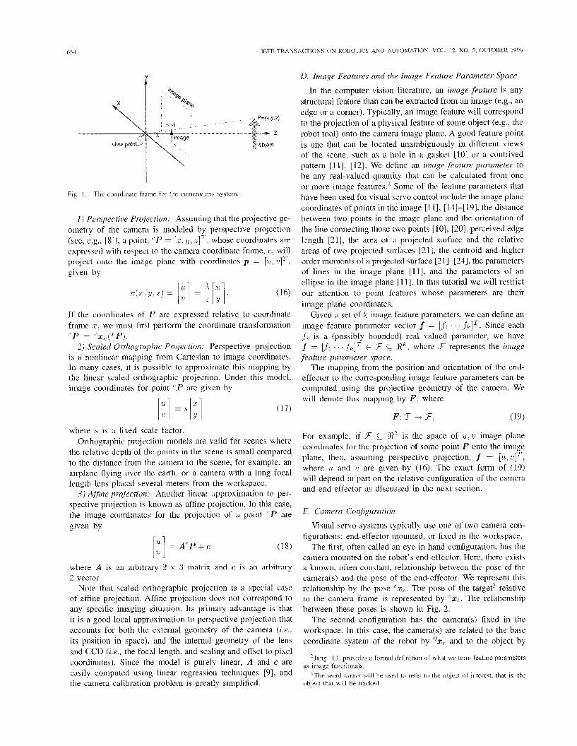
For each of the three projection models, we assign the camera coordinate system with the T C - and y-axes forming a basis for the image plane, the z-axis perpendicular to the image plane (along the optical axis), and with origin located at distance X behind the image plane, where X is the focal length of the camera lens. This is illustrated in Fig. 1.

654 IEEE TRANSACTIONS O N ROBOTICS AND AUTOMATION, VOL 12, NO 5 , OCTOBER 1996

i

Fig. 1. The coordinate frame for the carnerdlens \ystein.

I ) Perspective Projection: Assuming that the projective ge- ometry of the camera is modeled by perspective projection (see, e.g., [8]), a point, “ P = [ x , y j z]”: whose coordinates are expressed with respect to the camera coordinate frame, c, will project onto the image plane with coordinates p = [ I L , ~ ] ~ ,

given by

If the coordinates of I’ are expressed relative to coordinate frame x; we must first perform the coordinate transformation

2 ) Scaled Orthographic Projection: Perspective projection is a nonlinear mapping from Cartesian to image Coordinates. In many cases, it is possible to approximate this mapping by the linear scaled orthographic projection. Under this model, image coordinates for point ‘I‘ are given by

c p = ( -x , r (JP) .

D. Image Features and the Image Feature Parameter Space

In the computer vision literature, an image feature is any structural feature than can be extracted from an image (e.g., an edge or a corner). Typically, an image feature will correspond to the projection of a physical feature of some object (e.g., the robot tool) onto the camera image plane. A good feature point is one that can be located unambiguously in different views of the scene, such as a hole in a gasket [lo] or a contrived pattern [ l l ] , [12]. We define an image feature parameter to be any real-valued quantity that can be calculated from one or more image features.2 Some of the feature parameters that have been used for visual servo control include the image plane coordinates of points in the image [l I], [14]-[19], the distance between two points in the image plane and the orientation of the line connecting those two points [lo], [20], perceived edge length [21], the area of a projected surface and the relative areas of two projected surfaces [21], the centroid and higher order moments of a projected surface [2 11-[24], the parameters of lines in the image plane [ I l l , and the parameters of an ellipse in the image plane 1111. In this tutorial we will restrict our attention to point features whose parameters are their image plane coordinates.

Given a set of k image feature parameters, we can define an image feature parameter vector f = [ f l . . . f k I T . Since each ,f, is a (possibly bounded) real valued parameter, we have f = [ f l . . . f k , l T E 3 C Rk, where 3 represents the image feature parameter space.

The mapping from the position and orientation of the end- effector to the corresponding image feature parameters can be computed using the projective geometry of the camera. We will denote this mapping by F , where

F : I ---i 3. (19) where s is a fixed scale factor.

Orthographic projection models are valid for scenes where the relative depth of the points in the scene is small compared to the distance from the camera to the scene, for example, an airplane flying over the earth, or a camera with a long focal length lens placed several meters from the workspace.

3) Af$ne projection: Another linear approximation to per-

For example, if F C g2 is the space of ? L , U image plane coordinates for the projection of some point P onto the image plane, then, assuming perspective projection, f = [U, uIT: where 71 and ?I are given by (16). The exact form of (19) will depend in part on the relative configuration of the camera and end-effector as discussed in the next section.

spective projection is known as affine projection. In this case, the image coordinates for the projection of a point ‘ P are given by

[:] = A ‘ P + c (1 8)

where A is an arbitrary 2 x 3 matrix and c is an arbitrary 2-vector.

Note that scaled orthographic projection is a special case of affine projection. Affine projection does not correspond to any specific imaging situation. Its primary advantage is that it is a good local approximation to perspective projection that accounts for both the external geometry of the camera (i.e., its position in space), and the intemal geometry of the lens and CCD (i.e., the focal length, and scaling and offset to pixel coordinates). Since the model is purely linear, A and c are easily computed using linear regression techniques [9], and

E. Camera Configuration

Visual servo systems typically use one of two camera con- figurations: end-effector mounted, or fixed in the workspace.

The first, often called an eye-in-hand configuration, has the camera mounted on the robot’s end-effector. Here, there exists a known, often constant, relationship between the pose of the camera(s) and the pose of the end-effector. We represent this relationship by the pose ‘x,. The pose of the target3 relative to the camera frame is represented by ‘zt . The relationship between these poses is shown in Fig. 2.

The second configuration has the camera(s) fixed in the workspace. In this case, the camera(s) are related to the base coordinate system of the robot by ‘2, and to the object by

Jang [ 131 provides a formal definition of what we term feature parameters

3The word fcirwr will be used to refer to the obiect of interest. that is. the as image functionals.

the camera calibration problem is greatly simplified. object that wi l l he tracked

HUTCHINSON et a/ : TUTORIAL ON VISUAL SERVO CONTROL 655

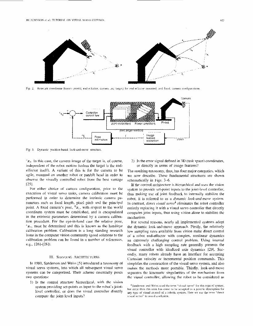
Fig. 2. Relevant coordinate frames (world, end-effector, camera and target) for end-effector mounted, and fixed, camera configurations

Fig. 3. Dynamic position-based look-and-move structure

(‘xt. In this case, the camera image of the target is, of course, independent of the robot motion (unless the target is the end- effector itself). A variant of this is for the camera to be agile, mounted on another robot or padtilt head in order to observe the visually controlled robot from the best vantage

For either choice of camera configuration, prior to the execution of visual servo tasks, camera calibration must be performed in order to determine the intrinsic camera pa- rameters such as focal length, pixel pitch and the principal point. A fixed camera’s pose, Oxc,. with respect to the world coordinate system must be established, and is encapsulated in the extrinsic parameters determined by a camera calibra- tion procedure. For the eye-in-hand case the relative pose, ‘xC. must be determined and this is known as the handleye calibration problem. Calibration is a long standing research issue in the computer vision community (good solutions to the calibration problem can be found in a number of references, e.g., [26]-[28]).

~ 5 1 .

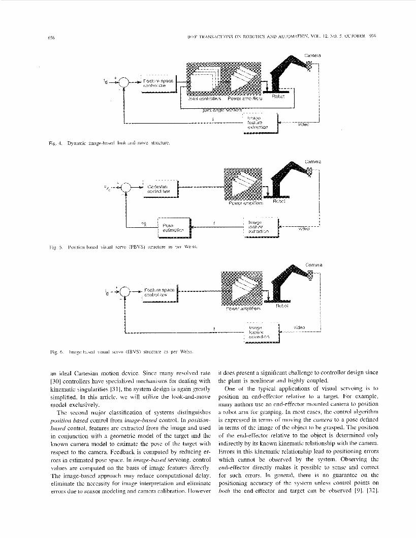
111. SERVOING ARCHITECTURES

In 1980, Sanderson and Weiss [5] introduced a taxonomy of visual servo systems, into which all subsequent visual servo systems can be categorized. Their scheme essentially poses two questions:

1) Is the control structure hierarchical, with the vision system providing set-points as input to the robot’s joint- level controller, or does the visual controller directly compute the joint-level inputs?

2) 1s the error signal defined in 3D (task space) coordinates,

The resulting taxonomy, thus, has four major categories, which we now describe. These fundamental structures are shown schematically in Figs. 3-6.

If the control architecture is hierarchical and uses the vision system to provide set-point inputs to the joint-level controller, thus making use of joint feedback to internally stabilize the robot, it is referred to as a dynamic look-and-move system. In contrast, direct visual servo4 eliminates the robot controller entirely replacing it with a visual servo controller that directly computes joint inputs, thus using vision alone to stabilize the mechanism.

For several reasons, nearly all implemented systems adopt the dynamic look-and-move approach. Firstly, the relatively low sampling rates available from vision make direct control of a robot end-effector with complex, nonlinear dynamics an extremely challenging control problem. Using internal feedback with a high sampling rate generally presents the visual controller with idealized axis dynamics [29]. Sec- ondly, many robots already have an interface for accepting Cartesian velocity or incremental position commands. This simplifies the construction of the visual servo system, and also makes the methods more portable. Thirdly, look-and-move separates the kinematic singularities of the mechanism from the visual controller, allowing the robot to be considered as

or directly in terms of image features?

4Sanderson and Weiss used the term “visual servo” for this type of system, but since then this term has come to be accepted as a generic description for any type o f visual control of a robotic system. Here we use the term “direct visual servo’’ to avoid confusion.

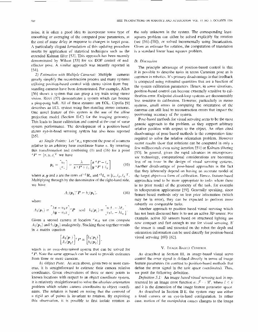
656 IFFE TRANSACTlONS O N ROBOTICS AND AUTOMArION, VOL 12. N O 5 , OCTOBER 1996

fd

Fig 4 Dynamic image-based look-and movc stiuLture

lrflagc feature

Fig. 5. Position-based visual servo (PBVS) structure as per Weiss

Camera

Fig. 6. Image-based visual servo (IBVS) structure as per Weiss.

an ideal Cartesian motion device. Since many resolved rate [30] controllers have specialized mechanisms for dealing with kinematic singularities [3 11, the system design is again greatly simplified. In this article, we will utilize the look-and-move model exclusively.

The second major classification of systems distinguishes position-based control from image-based control. In position- bused control, features are extracted from the image and used in conjunction with a geometric model of the target and the known camera model to estimate the pose of the target with respect to the camera. Feedback is computed by reducing er- rors in estimated pose space. In image-based servoing, control values are computed on the basis of image features directly. The image-based approach may reduce computational delay, eliminate the necessity for image interpretation and eliminate errors due to sensor modeling and camera calibration. However

it does present a significant challenge to controller design since the plant is nonlinear and highly coupled.

One of the typical applications of visual servoing is to position an end-effector relative to a target. For example, many authors use an end-effector mounted camera to position a robot arm for grasping. In most cases, the control algorithm is expressed in terms of moving the camera to a pose defined in terms of the image of the object to be grasped. The position of the end-effector relative to the object is determined only indirectly by its known kinematic relationship with the camera. Errors in this kinematic relationship lead to positioning errors which cannot be observed by the system. Observing the end-effector directly makes it possible to sense and correct for such errors. In general, there is no guarantee on the positioning accuracy of the system unless control points on both the end-effector and target can be observed [9], [32],

HUTCHINSON et a/: 'rUTORIA1L ON VISUAI. SERVO CONTROL 651

[33]. To emphasize this distinction, we refer to systems that only observe the target object as endpoint open-loop (EOL) systems, and systems that observe both the target object and the robot end-effector as endpoint closed-loop (ECL) systems. The differences between EOL and ECL systems will be made more precise in subsequent discussions.

It is usually possible to transform an EOL system to an ECL system simply by including direct observation of the end-effector or other task-related control points. Thus, from a theoretical perspective, it would appear that ECL systems would always be preferable to EOL systems. However, since ECL systems must track the end-effector as well as the target object, the implementation of an ECL controller often requires solution of a more demanding vision problem and places field-of-view constraints on the system that cannot always be satisfied.

IV. POSITION-BASED VISUAL SERVO CONTROL

We begin our discussion of visual servoing methods with position-based visual servoing. As described in the previous section, in position-based visual servoing, features are ex- tracted from the image and used to estimate the pose of the target with respect to the camera. Using these values, an error between the current and the desired pose of the robot is defined in the task space. In this way, position-based control neatly separates the control issues, namely the the computation of the feedback signal, from the estimation problems involved in computing position or pose from visual data.

We now formalize the notion of a positioning task as follows:

Definition 4.1: A positioning task is represented by a func- tion E : I + R"'. This function is referred to as the kinematic error ,function. A positioning task is fulfilled with the end- effector in pose 2, if E ( 2 , ) = 0.

If we consider a general pose x, for which the task is fulfilled, the error function will constrain some number, d 5 711; degrees of freedom of the manipulator. The value d will be referred to as the degree of the constraint. As noted by Espiau et ul. [ I l l , [34], the kinematic error function can be thought of as representing a virtual kinematic constraint between the end-effector and the target.

Once a suitable kinematic error function has been defined and the parameters of the functions are instantiated from visual data, a regulator is defined that reduces the estimated value of the kinematic error function to zero. This regulator produces at every time instant a desired end-effector velocity screw U E $2' that is sent to the robot control subsystem. For the purposes of this article, we use simple proportional control methods for linear and linearized systems to compute U [35]. Although there are formalized methods for developing such control laws, since the kinematic error functions are defined in Cartesian space, for most problems it i s possible to develop a regulator through geometric insight. The process is to first determine the relative motion that would fulfill the task, and then to write a control law that would produce that motion.

The remainder of the section presents various example problems that we have chosen to provide some insight into

ways of thinking about position-based control, and that will also provide useful comparisons when we consider image- based control in the next section. Section IV-A introduces several simple positioning primitives, based on directly ob- servable feature points, which can be compounded to achieve more complex positioning tasks. Next, Section IV-B describes positioning tasks based on the explicit estimation of the target object's pose. Finally, in Section IV-C, we briefly describe how point position and object pose can be computed using visual information from one or more cameras-the visual reconstruction problem.

A. Point-Feature Based Motions

We begin by considering a positioning task in which some point on the robot with end-effector coordinates, ' P , is to be brought to a fixed stationing point, S. visible in the scene. We refer to this as point-to-point positioning. In the case where the camera is fixed, the kinematic error function may be defined in base coordinates as

Epp(2,; s, " P ) = X " ( " P ) - s. (20)

Here, as in the sequel, the argument before the semicolon is the value to be controlled (in all cases, manipulator position) and the values after the semicolon parameterize the positioning task.

E,, defines a three degree of freedom kinematic constraint on the robot end-effector position. If the robot workspace is restricted to be 7 = @, this task can be thought of as a rigid link that fully constrains the pose of the end-effector relative to the target. When IT SE3, the constraint defines a virtual spherical joint between the object and the robot end-effector.

Let I = R3. We first consider the case in which one or more cameras calibrated to the robot base frame furnish an estimate, ' S . of the stationing point coordinates with respect to a camera coordinate frame. Using the estimate of the camera pose in base coordinates, 2'. from off-line calibration and (l), we have S = S,('S).

Since 7 = R3, the control input to be computed is the desired robot translational velocity, which we denote by u3 to distinguish it from the more general end-effector screw. Since (20) is linear in xf, it is well known that in the absence of outside disturbances, the proportional control law

will drive the system to an equilibrium state in which the value of the error function is zero [35]. The value k > 0 is a proportional feedback gain. Note that we have written 3, in the feedback law to emphasize the fact that this value is also subject to errors.

The expression (21) is equivalent to open-loop positioning of the manipulator using vision-based estimates of geome- try. Variations on this scheme are used by [36], [37]. In our simplified dynamics, the manipulator is stationary when ILJ = 0. Since the right hand side of the equation includes estimated quantities, it follows that errors in 3,, or "S

658 lEEE TRANSACTIONS ON ROBOTICS AND AUTOMATION, VOL. 12, NO. 5, OCTOBER 1996

(robot kinematics, camera calibration and visual reconstruction respectively) can lead to positioning errors of the end-effector.

Now, consider the situation when the cameras are mounted on the robot and calibrated to the end-effector. In this case, we can express (20) in end-effector coordinates

pEIIp(z,; s; ' P ) = ' P - 'zo(S). (22)

The camera(s) furnish an estimate of the stationing point, " S , which can be combined with information from the camera calibration and robot kinematics to produce S = (ke o 'kc)(?,!?). w e now compute

'213 = - k eElIp(kp; (& 0 "kC)("S) , " P ) = - k (?P- ('20 0 02' 0 % ) ( " S ) )

= -k( 'P - e k . c ( " s ) ) . (23)

Notice that the terms involving 2' have dropped out. Thus (23) is not only simpler, but positioning accuracy is also independent of the accuracy of the robot kinematics-a fundamental benefit of visual servoing.

All of the above formulations presume prior knowledge of " P and are therefore EOL systems. To convert them to ECL systems, we suppose that ' P is directly observed and estimated by the camera system. In this case, (21) and (23) can be written

A A

us = -k E p p ( d e ; k < : ( C s ) , "2J"P)) = -k 2J'P - ' S )

cu3 = - k 'Epp(k,;kc(Cs), % ( " P ) ) = -k ekc("P - 'S) (24)

(25)

respectively. We now see that u3 (respectively ' U S ) does not depend on 2, and is homogeneous in xc (respectively Hence, if 'S = ' P , then u3 = 0, independent of errors in the robot kinematics or the camera calibration. This is an important advantage for systems where a precise camerdend- effector relationship is difficult or impossible to determine off-line.

Consider now the full Cartesian problem where I C SE3, and the control input is the complete velocity screw U E R6. Since, the error functions presented above only constrain 3 degrees of freedom, the problem of computing U from the estimated error is under-determined. One way of proceeding is as follows. Consider the case of free standing cameras. Then in base coordinates we know that P = 213. Using (14), we can relate this to the end-effector velocity screw as follows:

P = 113 = A( P)u. (26)

Thus, if we could "solve for" IL in the above equation, we could effectively use the three-dimensional solution to arrive at the full Cartesian solution. Unfortunately, A is not square and therefore can cannot be inverted to solve for U . However, recall that the matrix right inverse for an m x n matrix M , n > m is defined as M+ = M T ( M M T ) - l . The right inverse computes the minimum norm vector which solves the original system of equations. Hence, we have

U A ( P ) + u ~ (27)

for free-standing cameras. Similar manipulations yield

for end-effector mounted cameras. Substituting the appropriate expression for u3 or eu, from the previous discussion leads to a form of proportional regulation for the Cartesian problem.

As a second example of feature-based positioning, consider that some point on the end-effector, " P , is to be brought to the line joining two fixed points S1 and S2 in the world. The shortest path for performing this task is to move " P toward the line joining SI and 5'2 along the perpendicular to the line. The error function describing this trajectory in base coordinates is:

Epz(2e;Sl,SZ,"P) = (S2 - SI) x ( ( zr ( 'P) - SI) X (5'2 - SI)). (29)

Notice that although E,l is a mapping from 7 to $ I 3 . placing a point on a line is a constraint of degree 2. From the geometry of the problem and the previous discussion, we see that defining

U = -kA(kr('P))+Epl(3,; gl, g2, ' P )

is a proportional feedback law for this problem.

the end-effector Suppose that now we apply this constraint to two points on

Eppl now defines a four degree of freedom positioning con- straint that aligns the points on the end-effector with those in target coordinates, and again no unique motion satisfies this kinematic error function. A geometrically straightforward solution is to compute a translation, T , which moves ' P I to the line through SI and S2. Simultaneously, we can choose a rotation, R which rotates eP2 about eP1 so that the line through ' P I and 'P2 becomes parallel to that through S1 and SZ.

In order to compute a velocity screw U = (T, R), we first note that the end-effector rotation matrix R, can be represented as a rotation through an angle B about an axis defined by a unit vector k [7]. In this case, the axis of rotation is

k = (S2 - SI) x [R,(eP2 - "PI)]

where the bar over expressions on the right denotes normal- ization to a unit vector. Hence, a natural feedback law for the rotational portion of the velocity screw is

R = -k1 t . (30)

Note the expression on the right hand size is the zero vector if the lines joining associated points are parallel as we desire.

The only complication to computing the translation portion of the vector is to realize that rotation introduces translation of points attached to the end-effector. Hence, we need to move "PI toward the goal line while compensating for the motion introduced by rotation. Based on the discussion above, we know the former is given by -Ep i (xe ; SI, 5'2, ' P I ) while

HUTCHINSON et al.: TUTORIAL ON VISUAL SERVO CONTROL 659

from (12) the latter is simply R x ze(‘Pl). Combining these two expressions, we have

Note that we are still free to choose translations along the line joining SI and S2 as well as rotations about it. Full six degree- of-freedom positioning can be attained by enforcing another point-to-line constraint using an additional point on the end- effector and an additional point in the world. Similar geometric arguments can be used to define a proportional feedback law.

These formulations can be adjusted for end-effector mounted camera and can be implemented as ECL or EOL systems. We leave these modifications as an exercise for the reader.

B. Pose-Based Motion

In the previous section, positioning was defined in terms of directly observable point features. When working with a priori known objects, it is possible to recover the pose of the object, xt, and to define stationing points with respect to object pose.

The methods of the previous section can be easily applied when object pose is available. For example, suppose tS is an arbitrary stationing point in a target object’s coordinate system, and that we can compute ‘xt using end-effenctor mounted camera(s). Then using (1) we can compute ‘5’ = ‘2t( tS) . This estimate can be used in any of the end-effector based feedback methods of the previous section in both ECL and EOL configurations. Similar remarks hold for systems utilizing free-standing cameras.

Given an object pose, it is possible to directly define positioning tasks in terms of that object pose. Let ‘x: be a desired stationing pose (rather than point as in the previous section) for the end-effector, and suppose the system employs free-standing cameras. We can define a positioning error

(Note that in order for this error function to be in accord with our definition of kinematic error we must select a parameterization of rotations which is 0 when the end-effector is in the desised position.)

Using feature information and the camera calibration, we can directly estimate xt = xc o ‘St . If we again represent the rotation in terms of a unit vector ‘ k, and rotation angle ‘ H , , we can define

where t , is the origin of the end-effector frame in base coordinates.

If we can also observe the end-effector and estimate its pose, ‘XP we can rewrite (32) as follows:

= (‘& 0 ‘2.0) 0 (OX(. 0 ‘&) 0 t2, = e&. 0 ex+ 0 t 2e - .

Once again we see that for an ECL system, both the robot kinematic chain and the camera pose relative to the base

coordinate system have dropped out of the error equation. Hence, these factors do not affect the positioning accuracy of the system.

The modifications of pose-based methods to end-effector based systems are completely straightforward and are left for the reader.

C. Estimation

A key issue in position-based visual servo is the estimation of the quantities used to parameterize the feedback. In this regard, position-based visual servoing is closely related to the problem of recovering scene geometry from one or more cam- era images. This encompasses problems including structure from motion, exterior orientation, stereo reconstruction, and absolute orientation. Unfortunately, space does not permit a complete coverage of these topics here and we have opted to provide pointers to the literature, except in the case of point estimation for two cameras, which has a straightforward solution. A comprehensive discussion of these topics can be found in a recent review article [38].

1) Estimation with a Single Camera: As noted previously, it follows from (16) that a point in a single camera im- age corresponds to a line in space. Although it is possible to perform geometric reconstruction using a single moving camera, the equations governing this process are often ill- conditioned, leading to stability problems [38]. Better results can be achieved if target image features have some internal structure, or the image features come from a known object. Below, we briefly describe methods for performing both point estimation and pose estimation with a single camera assuming such information is available.

a ) Single Points: Clearly, extra information is needed in order to reconstruct the Cartesian coordinates of a point in space from a single camera projection. This may come from additional measurable attributes, for example, in the case of a circular opening with known diameter d the image will be an ellipse. The ellipse can be described by five image feature parameters from which can be derived distance to the opening, and orientation of the plane containing the hole.

b) Object Pose: Object pose can be estimated if the vision system observes multiple point features on a known object. This is referred to as the pose estimation problem in the vision literature, and numerous methods for its solution have been proposed. These can be broadly divided into analytic solutions and least-squares solutions. Analytic solutions for three and four points are given by [39]-[43], and unique solutions exist for four coplanar, but not collinear, points. Least-squares solutions can be found in [44]-[50]. Six or more points always yield unique solutions and allow the camera calibration matrix to be computed. This can then be decomposed [48] to yield the target’s pose.

The general least-squares solution is a nonlinear optimiza- tion problem which has no known closed-form solution. In- stead, iterative optimization techniques are generally em- ployed. These techniques iteratively refine a nominal pose value using observed data (see [SI] for a recent review). Because of the sensitivity of the reconstruction process to

660 IEEE TRANSACTlONS ON KOBOTICS AND AUTOMATION, VOL. 12, NO. 5, OCTOBER 1996

noise, it is often a good idea to incorporate some type of smoothing or averaging of the computed pose parameters, at the cost of some delay in response to changes in target pose. A particularly elegant formulation of this updating procedure results by application of statistical techniques such as the extended Kalman filter [52]. This approach has been recently demonstrated by Wilson [53] for six DOF control of end- effector pose. A similar approach was recently reported in t541.

2) Estimation with Multiple Cameras: Multiple cameras greatly simplify the reconstruction process and many systems utilizing position-based control with stereo vision from free- standing cameras have been demonstrated. For example, Allen [36] shows a system that can grasp a toy train using stereo vision. Rizzi [37] demonstrates a system which can bounce a ping-pong ball. All of these systems are EOL. Cipolla [9] describes an ECL system using free-standing stereo cameras. One novel feature of this system is the use of the affine projection model (Section II-C) for the imaging geometry. This leads to linear calibration and control at the cost of some system performance. The development of a position-based stereo eye-in-hand servoing system has also been reported [551.

a ) Single Points: Let ax,l represent the pose of a camera relative to an arbitrary base coordinate frame a. By inverting this transformation and combining (1) and (16) for a point " P = [x,?/ ,zIT we have

where x, y and z are the rows of '.lR, and "ta = [ t r , C,, 1,IT. Multiplying through by the denominator of the right-hand side, we have

Al(P,)"P Z Y bl(P1). (36)

where

Given a second camera at location ' x , ~ we can compute A2 ( p 2 ) and b2 ( p 2 ) analogously. Stacking these together results in a matrix equation

which is an over-determined system that can be solved for " P . Note the same approach can be used to provide estimates from three or more cameras.

b ) Object Pose: As seen above, given two or more cam- eras, it is straightforward to estimate their camera relative coordinates. Given observations of three or more points in known locations with respect to an object coordinate system, it is relatively straightforward to solve the absolute orientation problem which relates camera coordinates to object coordi- nates. The solution is based on noting that the centroid of a rigid set of points is invariant to rotation. By exploiting this observation, it is possible to first isolate rotation as

the only unknown in the system. The corresponding least- squares problem can either be solved explicitly for rotation (see [56]-[58]), or solved incrementally using linearization. Given an estimate for rotation, the computation of translation is a standard linear least squares problem.

D. Discussion

The principle advantage of position-based control is that it is possible to describe tasks in terms Cartesian pose as is common in robotics. It's primary disadvantage is that feedback is computed using estimated quantities that are a function of the system calibration parameters. Hence, in some situations. position-based control can become extremely sensitive to cal- ibration error. Endpoint closed-loop systems are demonstrably less sensitive to calibration. However, particularly in stereo systems, small errors in computing the orientation of the cameras can still lead to reconstruction errors that impact the positioning accuracy of the system.

Pose-based methods for visual servoing seem to be the most generic approach to the problem, as they support arbitrary relative position with respect to the object. An often cited disadvantage of pose-based methods is the computation time required to solve the relative orientation problem. However recent results show that solutions can be computed in only a few milliseconds even using iteration [51] or Kalman filtering [53]. In general, given the rapid advances in microproces- sor technology, computational considerations are becoming less of an issue in the design of visual servoing systems. Another disadvantage of pose-based approaches is the fact that they inherently depend on having an accurate model of the target object-a form of calibration. Hence, feature-based approaches tend to be more appropriate to tasks where there is no prior model of the geometry of the task, for example in teleoperation applications [59]. Generally speaking, since feature-based methods rely on less prior information (which may be in error), they can be expected to perform more robustly on comparable tasks.

Another approach to position-based visual servoing which has not been discussed here is to use an active 3D sensor. For example, active 3D sensors based on structured lighting are now compact and fast enough to use for visual servoing. If the sensor is small and mounted on the robot the depth and orientation information can be used directly for position-based visual servoing [60]-[621.

V. IMAGE-BASED CONTROL

As described in Section 111, in image-based visual servo control the error signal is defined directly in terms of image feature parameters (in contrast to position-based methods that define the error signal in the task space coordinates). Thus, we posit the following definition.

Definition 5.1: An image-based visual servoing task is rep- resented by an image error function e: 3 + R'. where I < k and k is the dimension of the image feature parameter space.

As described in Section II-E, the system may use either a fixed camera or an eye-in-hand configuration. In either case, motion of the manipulator causes changes to the image

HIJTCkIINSON c’f d: TUTORIAL ON VISUAL SERVO CONTROL 66 I

observed by the vision system. Thus, the specification of an image-based visual servo task involves determining an appro- priate error function e , such that when the task is achieved, e = 0. This can be done by directly using the projection equations (16), or via a “teach by showing” approach in which the robot is moved to a goal position and the corresponding image is used to compute a vector of desired image feature parameters, fd. If the task is defined with respect to a moving object, the error, e . will be a function, not only of the pose of the end-effector, but also of the pose of the moving object.

Although the error, e , is defined on the image parameter space, the manipulator control input is typically defined either in joint coordinates or in task space coordinates. Therefore, it is necessary to relate changes in the image feature parameters to changes in the position of the robot. The image Jacobian, introduced in Section V-A, captures these relationships. We present an example image Jacobian in Section V-B. In Section V-C, we describe methods that can be used to “invert” the image Jacobian, to derive the robot velocity that will produce the desired change in the image. Finally, in Sections V-D and V-E we describe how controllers can be designed for image-based systems.

A. The Image Jacobian

Let T represent coordinates of the end-effector in some parameterization of the task space 7 and i represent the corresponding end-effector velocity (note, i is a velocity screw, as defined in Section 11-B). Let f represent a vector of image feature parameters and the corresponding vector of image feature parameter rates of change’. The image Jacobian, ?7?>, is a linear transformation from the tangent space of 7 at r to the tangent space of .F at J. In particular

f = J,;(r)i-

where *7,> E RRkXnL, and

J,; ( r ) = [ g] =

B. An Example Image Jacobian

Suppose that the end-effector is moving with angular ve- locity ‘12, = [w,, w y , w.] and translational velocity ‘T, = [T,. T?,) TZ] (as described in Section 11-B) both with respect to the camera frame in a fixed camera system. Let P be a point rigidly attached to the end-effector. The velocity of the point P , expressed relative to the camera frame, is given by

‘’P = ‘R, x ‘ P + ‘T?. (39)

To simplify notation, let ‘ P = [x. y. z]*. Substituting the perspective projection equations (16) into (10) and (1 l), we can write the derivatives of the coordinates of “ P in terms of the image feature parameters U , ? ) as

(40)

(41)

(42)

Cl 6 .i. = Z W ~ - -U, + Tr

G = - w , - ZW, +Ty x

U Z

x x z z = -(vw, - uw,) + T,.

Now, let f = [U, U]*. as above and using the quotient rule,

(43 ) 2.r. - 22.

i l=A- 2 2

(44)

Similarly

x u - A 2 - v2 uv i i = -T z Y - -T, + wT + -wY x +uw,. (46)

(37) Finally, we may rewrite these two equations in matrix form to obtain

Recall that m, is the dimension of the task space, 7. Thus the number of columns in the image Jacobian will vary depending on the task.

The image Jacobian was first introduced by Weiss et al. [21 J , who referred to it as the feature seizsitivity matrix. It is also referred to as the interaction matrix [ 111 and the B matrix [16], [17]. Other applications of the image Jacobian include

The relationship given by (37) describes how image feature parameters change with respect to changing manipulator pose. In visual servoing we are interested in determining the ma- nipulator velocity, i , required to achieve some desired value of i. This requires solving the system given by (37). We will discuss this problem in Section V-C, but first we present an example image Jacobian.

~101, 1141, [151, ~ 4 1 .

‘If the image featurc parameters are point coordinates these rates arc image planc point velocities.

x [;I = [, 0

0 x -

z

U

z u

?1 v

z x

x2 + u2 x

x UV -

(47)

which relates image-plane velocity of a point to the relative velocity of the point with respect to the camera. Alternative derivations for this example can be found in a number of references including [63], [64].

It is straightforward to extend this result to the general case of using k / 2 image points for the visual control by simply stacking the Jacobians for each pair of image point coordinates; see (48), shown at the bottom of the next page.

Finally, note that the Jacobian matrices given in (47) and (48) are functions of z,, the distance to the point being imaged. For a fixed camera system, when the target is the end-effector these x values can be computed using the forward kinematics of the robot and the camera calibration information. For an eye-in-hand system, determining z can be more difficult, and this problem is discussed further in Section V-F.

662 IEEE TRANSACTIONS ON ROBOTICS AND AUTOMATION, VOL. 12, NO. 5 , OCTOBER 1996

-U

U x 0 0 -0

C. Using the Image Jacobian to Compute End-Effector Velocity

The results of the previous sections show how to relate robot end-effector motion to perceived motion in a camera image. However, visual servo control applications typically require the reverse-computation of i given f as input. There are three cases that must be considered: k = 7n, k < m, and k. > m. We now discuss each of these.

When k = m, and J , is nonsingular, J,' exists. Therefore, in this case, r = Ji'f. Such an approach has been used by Feddema [20], who also describes an automated approach to image feature selection in order to minimize the condition number of J u .

When k # m: J L 1 does not exist. In this case, assuming that J , , is full rank (i.e., rank(J,,) = min(k, m ) ) , we can compute a least squares solution, which, in general, is given by

i = Jrff + ( I - J ; f J , , ) b (49)

where Jrf is a suitable pseudoinverse for J,, and b is an arbitrary vector of the appropriate dimension. The least squares solution gives a value f o r i that minimizes the norm l l f - J l , ill .

We first consider the case k > m; that is , there are more feature parameters than task degrees of freedom. By the implicit function theorem [65], if, in some neighborhood of r ,m 5 k: and rank(d,,) = m (i.e., J,: is full rank), we can express the coordinates fTrL+1 Jllc as smooth functions of f l . . , fnL . From this, we deduce that there are k - m redundant visual features. Typically, this will result in a set of inconsistent equations (since the k visual features will be obtained from a computer vision system and are likely to be noisy). In this case, the appropriate pseudoinverse is given by

J: = (J:J?,)-'J;. (50)

Here, we have ( I - J:J,) = 0 (the rank of the null space of J , is 0, since the dimension of the column space of J , : m, equals rank( J ( , ) ) . Therefore, the solution can be written more concisely as

r = J : f . (5 1)

Such approaches have been used by Hashimoto [lS] and Jang [661.

When k < n, the system is under-constrained. In the visual servo application, this implies that we are not observing enough features to uniquely determine the object motion i,

-0 0 0 U V

-x

i.e., there are certain components of the object motion that can not be observed. In this case, the appropriate pseudoinverse is given by

In general, for k < m, ( I - S T J , ) # 0, and all vectors of the form ( I - J ; J , ) b lie in the null space of J,, and correspond to those components of the object velocity that are unobservable. In this case, the solution is given by (49). For example, as shown in [64], the null space of the image Jacobian given in (47), is spanned by the four vectors

In some instances, there is a physical interpretation for the vectors that span the null space of the image Jacobian. For example, the vector [U. v , A, 0, 0, 0IT reflects that the motion of a point along a projection ray cannot be observed. The vector [O, 0, 0, U , v , A]' reflects the fact that rotation of a point on a projection ray about that projection ray cannot be observed. Unfortunately, not all basis vectors for the null space have such an obvious physical interpretation. The null space of the image Jacobian plays a significant role in hybrid methods, in which some degrees of freedom are controlled using visual servo, while the remaining degrees of freedom are controlled using some other modality [14].

D. Resolved-Rate Methods

The earliest approaches to image-based visual servo control [lo], [21] were based on resolved-rate motion control [30], which we will briefly describe here. Suppose that the goal of a particular task is to reach a desired image feature parameter vector, fd. If the control input is defined as in Section IV to be an end-effector velocity, then we have U = r , and assuming for the moment that the image Jacobian is square and nonsingular,

If we define the error function as e(f) = f d - f , a simple proportional control law is given by

x 21

0

-

x 2 k / 2

0

0

x 21 -

0

x

A2 + up x

UlUl

x __

x2 x

x k / 2 k / 2

HUTCHlNSON et ut.: TIJTORlAL ON VISUAL SERVO CONTROL 663

where K is a constant gain matrix of the appropriate di- mension. For the case of a nonsquare image Jacobian, the techniques described in Section V-C would be used to compute for U . Similar results have been presented in [14], [15]. More advanced techniques based on optimal control are discussed in 1161.

E. Examde Servoinn Tasks

proof proceeds as follows. The origin of the coordinate frame for the left camera, together with the projections of S1 and S2 onto the left image forms a plane. Likewise, the origin of the coordinate frame for the right camera, together with the projections of SI and onto the right image forms a plane. The intersection of these two planes is exactly the line joining SI and S2 in the workspace. When P lies on this line, it must lie simultaneously in both of these planes, and therefore, must -

In this section, we revisit some of the problems introduced in Section IV-A and describe image-based solutions for these problems. In all cases, we assume two fixed cameras are observing the scene.

1) Point to Point Positioning: Consider the task of bring- ing some point P on the manipulator to a desired stationing point S. The kinematic error function was given in (20). If two cameras are viewing the scene, a necessary and sufficient condition for P and S to coincide in the workspace is that the projections of P and S coincide in each image.

If we let [U’, 71‘1~ and [ur, vrIT be the image coordinates for the projection of P in the left and right images, respectively, then we may take f = [ , ~ ‘ , d , u ~ , v ~ ] ~ . If we let ‘T = R,?, then in (19), F is a mapping from 7 to R4.

Let the projection of S have coordinates [U:, TI,:] and [7~:, ?I;]

in the left and right images. We then define the desired feature vector to be f C i = [U; . U;, ,U:, yielding

The image Jacobian for this problem can be constructed by “stacking” (47) for each camera. Note, however, that a coordinate transformation must be used for each camera in order to relate the end-effector velocity screw in camera coordinates to the robot reference frame.

Unfortunately, the resulting Jacobian matrix cannot be in- verted as it is a matrix with four rows and six columns which is of rank three. This is a reflection of the fact that although two cameras provide four measurements, the point observed has only three degrees of freedom. Hence, one measurement value is redundant, or equivalently the observations are constrained to lie on a three-dimensional subspace of four-dimensional measurement space. The constraint defining this subspace is known as the epipolar constraint in the vision literature [67].

There are a variety of methods for dealing with this problem. The simplest is to note that most stereo camera systems are arranged so that the camera z (horizontal) axes are roughly co-planar. In this case, the redundant information is largely concentrated in the y (vertical) coordinates, and so one can be discarded. Doing so removes a row from the Jacobian, and the resulting matrix has a well-defined inverse.

2) Point to Line Positioning: Consider again the task in which some point P on the manipulator end-effector is to be brought to the line joining two fixed points SI and S z in the world. The kinematic error function is given by (29).

If two cameras are viewing the workspace, it can be shown that a necessary and sufficient condition for P to be colinear with the line joining S1 and 5 2 is that the projection of P be colinear with the projections of the points S1 and sz in both images (for nondegenerate camera configurations). The

be colinear with the the projections of the points S1 and S2

in both images. We now tum to conditions that determine when the pro-

jection of P is colinear with the projections of the points SI and Sz? and will use the knowledge that three vectors are coplanar if and only if their scalar triple product is zero. For the left image, let the projection of SI have image coordinates [U;, 41. the projection of Sz have image coordinates [ U ; , wk], and the projection of P have image coordinates [d. U‘]. If the three vectors from the origin of the left camera to these image points are coplanar, then the three image points are colinear. Thus, we construct the scalar triple product

and proceeding in a similar fashion for the right image, derive from which we construct the error function

where f = [U‘, d, U”; uUTlT. It is important to note that this error is a linear projection of the image coordinates of the point P , and hence the Jacobian is also a linear transformation of the image Jacobian for P . To make this explicit, let $;(E‘) denote the image Jacobian for P in the left camera. Then it follows that the image Jacobian for efr is

The derivation of the image Jacobian in the right camera is similar. The full Jacobian is the “stack’ consisting of Jhi and -7Ll multiplied with a coordinate transformation to relate the end-effector velocity screw in robot coordinates to the equivalent motion in the camera coordinate frame. Note that given a second point on the end-effector, a four degree of freedom positioning operation can be defined by simply stack- ing the two “point-to-line” errors and their image Jacobians. Likewise, choosing yet another point in the world and on the manipulator, and setting up an additional independent “point-to-line” problem yields a rigid six degree of freedom positioning problem

F. Discussion

It is interesting to note that image-based solutions to the point-to-line problem discussed above perform with an ac- curacy that is independent of calibration. This follows from

664 IEEE TRANSACTIONS ON ROBOTICS AND AUTOMATION, VOL 12, NO 5 , OCTOBER 1996

the fact that by construction, when the image error function is zero, the kinematic error must also be zero. Even if the hand-eye system is miscalibrated, if the feedback system is asymptotically stable, the image error will tend to zero, and hence so will the kinematic error. This is not the case with the position-based system described in Section IV [68]. Thus, one of the chief advantages to image-based control over position- based control is that the positioning accuracy of the system is less sensitive to camera calibration errors.

There are also often computational advantages to image- based control, particularly in ECL configurations. For example, a position-based relative pose solution for an ECL single- camera system must perform two nonlinear least squares optimizations in order to compute the error function. The comparable image-based system must only compute a sim- ple image error function, an inverse Jacobian solution, and possibly a single position or pose calculation to parameterize the Jacobian. In practice, as described in Section V-B, the un- known parameter for Jacobian calculation is distance from the camera. Some recent papers present adaptive approaches for estimating this depth value [16], or develop feedback methods which do not use depth in the feedback formulation [69].

One disadvantage of image-based methods compared to position-based methods is the presence of singularities in the feature mapping function which reflect themselves as unstable points in the inverse Jacobian control law. These instabili- ties are often less prevalent in the equivalent position-based scheme. Returning again to the point-to-line example, the Jacobian calculation becomes singular when the two stationing points are coplanar with the optical centers of both cameras. In this configuration, rotations and translations of the setpoints in the plane are not observable. This singular configuration does not exist for the position-based solution.

In the above discussion we have referred to f as the desired feature parameter vector, and implied that it is a constant. If it is a constant then the robot will move to the desired pose with respect to the target. If the target is moving the system will endeavor to track the target and maintain relative pose, but the tracking performance will be a function of the system dynamics, as discussed below in Section VII. However many tasks can be described in terms of the motion of image features, for instance by aligning visual cues within the scene. Jang et ul. [66] describe a generalized approach to servoing on image features, with trajectories specified in feature space which results in trajectories (tasks) that are independent of target geometry. Feddema [lo] also uses a feature space trajectory generator to interpolate feature parameter values due to the low update rate of the vision system used. Skaar et al. [IS] describe the example of a lDOF robot catching a ball by observing visual cues such as the ball, the arm’s pivot point, and another point on the arm. The interception task can then be specified, even if the relationship between camera and arm is not known a priori.

VI. IMAGE FEATURE EXTRACTION AND TRACKING

Irrespective of the control approach used, a vision system is required to extract the information needed to perform the

servoing task. Hence, visual servoing pre-supposes the solution to a set of potentially difficult static and dynamic vision problems. To this end many reported implementations contrive the vision problem to be simple: e.g. painting objects white, using artificial targets, and so forth [lo], [14], [37], [70]. Other authors use extremely task-specific clues: e.g. Allen [36] uses motion detection for locating a moving object to be grasped, and a fruit picking system looks for the characteristic fruit color. A review of tracking approaches used by researchers in this field is given in [3].

In less structured situations, vision has typically relied on the extraction of sharp contrast changes, referred to as “comers” or “edges”, to indicate the presence of object boundaries or surface markings in an image. Processing the entire image to extract these features necessitates the use of extremely high- speed hardware in order to work with a sequence of images at camera rate. However not all pixels in the image are of interest, and computation time can be greatly reduced if only a small region around each image feature is processed. Thus, a promising technique for making vision cheap and tractable is to use window-based tracking techniques [4], [37], [71]. Window-based methods have several advantages, among them: computational simplicity, little requirement for special hard- ware, and easy reconfiguration for different applications. We note, however, that initial positioning of each window typically presupposes an automated or human-supplied solution to a potentially complex vision problem.

This section describes a window-based approach to tracking features in an image. The methods are capable of tracking a number of point or edge features at frame rate on a workstation computer and require a framestore, no specialized image pro- cessing hardware, and have been incorporated into a publicly available software “toolkit” [4]. A discussion of methods which use specialized hardware combined with temporal and geometric constraints can be found in [67]. The remainder of this section is organized as follows. Section VI-A describes how window-based methods can be used to implement fast detection of edge segments, a common low-level primitive for vision applications. Section VI-B describe an approach based on temporally correlating image regions over time. VI-C describes some general issues related to the use of temporal and geometric constraints, and Section VI-D briefly summarizes some of the issues surrounding the choice of a feature extraction method for tracking.

A. Feature Bused Methods

In this section, we illustrate how window-based processing techniques can be used to perform fast detection of isolated straight edge segments of fixed length. Edge segments are intrinsic to applications where man-made parts contain comers or other patterns formed from physical edges.

Images are comprised of pixels organized into a two- dimensional coordinate system. We adopt the notation 1(x, t ) to denote the pixel at location 2 [U, .IT in an image captured at time k . A window can be thought of as a two-dimensional array of pixels related to a larger image by an invertible mapping from window coordinates to image coordinates. We

HIJTCHINSON et al TUTORlAl ON VISUAI. SERVO CONTROL 665

consider rigid transformations consisting of a translation vector c = [J , 1/]' and a rotation 8. A pixel value at x = [U. U]'' in window coordinates is related to the larger image by

W ( z : c, 0, t ) = I ( c + B ( Q ) X , t ) (60)

where R is a two dimensional rotation matrix. We adopt the conventions that x = 0 is the center of the window, and the set X represents the set of all values of x.

Window-based tracking algorithms typically operate in two stages. In the first stage, one or more windows are acquired using a nominal set of window parameters. The pixel values for all x E X are copied into a two-dimensional array that is subsequently treated as a rectangular image. Such acquisitions can be implemented extremely efficiently using line-drawing and region-fill algorithms commonly developed for graphics applications [72]. In the second stage, the windows are pro- cessed to locate image features and from their parameters a new set of window parameters, 0 and e, are computed. These parameters may be modified using external geometric constraints or temporal prediction, and the cycle repeats.

We consider an edge segment to be characterized by three parameters in the image plane: the PL and 7) coordinates of the center of the segment, and the orientation of the segment relative to the image plane coordinate system. These values correspond directly to the parameters of the acquisition window used for edge detection. Let us first assume we have correct prior values e- = ( P L - , v ) and Q- for an edge segment. A window, W - (x) = W ( x ; e - , Q-, t ) . extracted with these parameters would then have a vertical edge segment within it.

Isolated step edges can be localized by determining the location of the maximum of the first derivative of the signal 1641, [67], [731. Let c be a l-dimensional edge detection kernel arranged as a single row. The convolution W,(x) = (W- ~r P)(z) will have a response curve in each row which peaks at the location of the edge. Summing each column of W1 superimposes the peaks and yields a one-dimensional response curve. If the estimated orientation, 0- , was correct, the maximum of this response curve determines the offset of the edge in window coordinates. By interpolating the response curve about the maximum value, sub-pixel localization of the edge can be achieved. Here, e is taken to be a 1-dimensional Prewitt operator [64] which, although not optimal from a signal processing point of view, is extremely fast to execute on simple hardware.

If the 0- was incorrect, the response curves in W1 will deviate slightly from one another and the superposition of these curves will form a lower and less sharp aggregate curve. Thus, maximizing the maximum value of the aggregate response curve is a way to determine edge orientation. This can be approximated by performing the detection operation on windows acquired at 8- as well as two bracketing angles 8- 5 a and performing quadratic interpolation on the maxima of the corresponding aggregate response curves. Computing the three oriented edge detectors is particularly simple if the range of angles is small. In this case, a single window is processed with the initial convolution yielding W1. Three aggregate response curves are computed by summing along

the columns of W1 and along diagonals corresponding to angles of fa. The maxima of all three curves are located and interpolated to yield edge orientation and position. Thus, for the price of one window acquisition, one complete 1- dimensional convolution, and three column sums, the vertical offset So and the orientation offset 60 can be computed. Once these two values are determined, the state variables of the acquisition window are updated as

8+ = e - + s o U+ = c - 60 sin(e+) v+ = ? I - + S O C O S ( 0 + ) .

An implementation of this method [4] has shown that localizing a 20 pixel long edge using a Prewitt-style mask 15 pixels wide searching k10 pixels and ~ t 1 5 degrees takes 1.5 ms on a Sun Sparc I1 workstation. At this rate, 22 edge segments can be tracked simultaneously at 30 Hz, the video frame rate used. Longer edges can be tracked at comparable speeds by sub-sampling along the edge.

Clearly, this edge-detection scheme is susceptible to mis- tracking caused by background or foreground occluding edges. Large acquisition windows increase the range of motions that can be tracked, but reduce the tracking speed and increase the likelihood that a distracting edge will disrupt tracking. Likewise, large orientation brackets reduce the accuracy of the estimated orientation, and make it more susceptible to edges that are not closely oriented to the underlying edge.

There are several ways of increasing the robustness of edge tracking. One is to include some type of additional information about the edges being tracked such as the sign or absolute value of the edge response. For more complex edge-based detection, collections of such oriented edge detectors can be combined to verify the location and position of the entire feature. Some general ideas in this direction are discussed in Section VI-C.

B. Area-Based Methods

Edge-based methods tend to work well in environments in which man-made objects are to be tracked. If, however, the desired feature is a specific pattern, then tracking can be based on matching the appearance of the feature (in terms of its spatial pattern of gray-values) in a series of images, and exploiting its temporal consistency-the observation that the appearance of small region in an image sequence changes little. Such techniques are well described in image registration literature and have been applied to other computer vision problems such as stereo matching and optical flow.

Consider only windows that differ in the location of their center. We assume some reference window was acquired at time t at location c. Some small time interval, 7 , later, a candidate window of the same size is acquired at location c + d . The correspondence between these two images is given by some similarity measure

O ( d ) = f ( ( W ( z ; c, i ) ) - W ( x ; c + d , t + 7))1u(x) , X E ' Y

T > O (61)

666 IEEE TRANSACTIONS ON ROBOTICS AND AUTOMATION, VOL. 12, NO. 5 , OCTOBER 1996

where w( 8 ) is a weighting function over the image region and f ( . ) is a scalar function. Commonly used functions include , f ( x ) = 1x1 for sum of absolute values (SAD) and f(x) = x2 for sum of squared differences (SSD).

The aim is to find the displacement, d , that minimizes O ( d ) . Since images are inherently discrete, a natural solution is to select a finite range of values D and compute

d = min q d ) . drD

The advantage of a complete discrete search is that the true minimum over the search region is guaranteed to be found. However, the larger the area covered, the greater the computational burden. This burden can be reduced by performing the optimization starting at low resolution and proceeding to higher resolution, and by ordering the candidates in D from most to least likely and terminating the search once a candidate with an acceptably low SSD value is found [17]. Once the discrete minimum is found, the location can be refined to sub-pixel accuracy by interpolation of the SSD values about the minimum. Even with these improvements, [ 171 reports that a special signal processor is required to attain frame-rate performance.

It is also possible to solve (61) using continuous optimiza- tion methods [4] [74]-[761. The solution begins by expanding W ( z ; c , t ) in a Taylor series about (c , t ) yielding

W ( z ; c + d, t + ?-)

N W ( ~ ; ~ , t ) f W z ( z ) dx+W,(z) dy+Wt(z)r

where W , I W , and W, are respectively the horizontal and ver- tical spatial, and temporal derivatives of the image computed using convolution as follows:

Substituting into (61) yields

O(d) = (Wz(x) dz+W,(x) d y + W + ( 2 ) r ) 2 w ( 2 ) . (62) X t ’ Y

Define

Expression (62) can now be written more concisely as

O ( d ) = (g(2) ’ d + h(2)?- )2 . X E X

Notice 0 is now a quadratic function of d . Computing the derivatives of 0 with respect to the components of d, setting the result equal to zero, and rearranging yields a linear system of equations:

r 1

Solving for d yields an estimate, d of the offset that would cause the two windows to have maximum correlation. We then compute c+ = c- + d yielding the updated window location for the next tracking cycle. This is effectively a proportional control algorithm for the “servoing” the location of an acquisition to maintain the best match with the reference window over time.

In practice this method will only work for small motions (it is mathematically correct only for a fraction of a pixel). This problem can be alleviated by first performing the opti- mization at low levels of resolution, and using the result as a seed for computing the offset at higher levels of resolution. For example, reducing the resolution by a factor of two by summing groups of four neighboring pixels doubles the maximum displacement between two images. It also speeds up the computations since fewer operations are needed to compute d for the smaller low-resolution image.

Another drawback of this method is the fact that it relies on an exact match of the gray values-changes in contrast or brightness can bias the results and lead to mistracking. Thus, it is common to normalize the images to have zero mean and consistent variance. With these modifications, it is easy to show that solving (64) is equivalent to maximizing the correlation between the two windows [74].

Continuous optimization has two principle advantages over discrete optimization. Firstly, a single updating cycle is usually faster to compute. For example, (64) can be computed and solved in less than 5 ms on a Sparc I1 computer [4]. Secondly, it is easy to incorporate other window parameters such as rotation and scaling into the system without greatly increasing the computation time [41, [76]. Thus, SSD methods can be used to perform template matching as well as tracking of image regions.

C. Feature Prediction

Window-based trackmg implicitly assumes that the inter- frame motions of the tracked feature do not exceed the size of search window, or, in the case of continuous optimization, a few pixels from the expected location of the image region. In the simplest case, the previous location of the image feature can be used as a predictor of its current location. Unfortunately, as feature velocity increases the search window must be enlarged which adversely affects computation time.

The robustness and speed of tracking can be significantly increased with knowledge about the motion of the observed features, which may be due to the camera and/or target moving. For example, given knowledge of the image feature location xt at time t , Jacobian J , , the end-effector velocity ut, and the inter-frame time r, the expected location of the search windows can be computed, assuming no target motion, by the prediction

f t t 7 = f t + rJvut.

Likewise, if the dynamics of a moving object are known, then it is possible to use this information to enhance tracking performance. For example, Rizzi [37] describes the use of a Newtonian flight dynamics model to make it possible to track a

HUTCHINSON ef ul.: TUTORIAL ON VISIJAL SERVO CONTROL 667

ping-pong ball during flight. Predictors based on (II -113 tracking filters and Kalman filters have also been used [36], [53], [67].

D. Discussion

Prior to executing or planning visually controlled motions, a specific set of visual features must be chosen. Discussion of the issues related to feature selection for visual servo control applications can be found in [20], [21]. The “right” image feature tracking method to use is extremely application dependent. For example, if the goal is to track a single special pattern or surface marking that is approximately planar and moving at slow to moderate speeds, then area-based tracking is appropriate. It does not require special image structure (e.g. straight lines), is robust to large set of image distortions, and for small motions can be implemented to run at frame rates.

In comparison to the edge detection methods described above, area-based tracking is sensitive to occlusions and background changes (if the template includes any background pixels). Thus, if a task requires tracking several occluding contours of an object with a changing background, edge-based methods are clearly faster and more robust.

In many realistic cases, neither of these approaches by themselves yields the robustness and performance desired. For example, tracking occluding edges in an extremely cluttered environment is sure to distract edge tracking as “better” edges invade the search window, while the changing background would ruin the SSD match for the region. Such situations call for the use of more global task constraints (e.g. the geometry of several edges), more global tracking (e.g. extended contours or snakes [77]), or improved or specialized detection methods.

To illustrate these tradeoffs, suppose a visual servoing task relies on tracking the image of a circular opening over time. In general, the opening will project to an ellipse in the camera. There are several candidate algorithms for detecting this ellipse and recovering its parameters:

1) If the contrast between the interior of the opening and area around it is high, then binary thresholding followed by a calculation of the first and second central moments can be used to localize the feature [37].

2) If the ambient illumination changes greatly over time, but the brightness of the opening and the brightness of the surrounding region are roughly constant, a circular template could be localized using SSD methods aug- mented with brightness and contrast parameters. In this case, (61) must also include parameters for scaling and aspect ratio [4].

3) The opening could be selected in an initial image, and subsequently located using SSD methods. This differs from the previous method in that this calculation does not compute the center of the opening, only its correlation with the starting image. Although useful for servoing a camera to maintain the opening within the field of view, this approach is probably not useful for manipulation tasks that need to attain a position relative to the center of the opening.

4) If the contrast and background are changing, the opening could be tracked by performing edge detection and

fitting an ellipse to the edge locations. In particular, short edge segments could be located using the techniques described in Section VI-A. Once the segments have been fit to an ellipse, the orientation and location of the segments would be adjusted for the subsequent tracking cycle using the geometry of the ellipse.

During task execution, other problems arise. The two most common problems are occlusion of features and visual singu- larities. Solutions to the former include intelligent observers that note the disappearance of features and continue to predict their locations based on previously observed motion [37], or redundant feature specifications that can perform even with some loss of information. Solution to the latter require some combination of intelligent path planning and/or intelligent ac- quisition and focus-of-attention to maintain the controllability of the system.

It is probably safe to say that fast and robust image process- ing presents the greatest challenge to general-purpose hand-eye coordination. As an effort to help overcome this obstacle, the methods described above and other related methods have been incorporated into a publicly available software “toolkit.” The interested reader is referred to [4] for details.

VII. DISCUSSION

This paper has presented a tutorial introduction to robotic visual servo control, focusing on the relevant fundamentals of coordinate transformations, image formation, feedback al- gorithms, and visual tracking. In the interests of space and clarity, we have concentrated on presenting methods that are well-represented in the literature, and that can be solved using relatively straightforward techniques. The reader interested in a broader overview of the field or interested in acquiring more detail on a particular area is invited to consult the references we have provided. Another goal has been to establish a consistent nomenclature and to summarize important results here using that notation.

Many aspects of the more general problem of vision-based control of motion have necessarily been omitted or abbreviated to a great degree. One important issue is the choice between using an image-based or position-based system. Many systems based on image-based and position-based architectures have been demonstrated, and the computational costs of the two approaches seem to be comparable and are easily within the capability of modem computers. In many cases the motion of a target, for example an object on a conveyer, is most naturally expressed in a Cartesian reference frame. For this reason, most systems dealing with moving objects ([36], [37]) have used position-based methods. Although there has been recent progress in understanding image plane dynamics [22], the design of stable, robust image-based servoing systems for capturing moving objects has not been fully explored.

In general, the accuracy of image-based methods for static positioning is less sensitive to calibration than comparable position-based methods, however image-based methods re- quire online computation of the image Jacobian. Unfortu- nately, this quantity inherently depends on the distance from the camera to the target which, particularly in a monocular

668 IEEE TRANSACTIONS ON ROBOTICS AND AUTOMATION, VOL. 12, NO 5, OCTOBER 1996

system, is difficult to compute. Many systems utilize a constant image Jacobian, which is computationally efficient, but valid only over a small region of the task space6. Other systems have resorted to performing a partial pose estimation [lo], adaptive depth estimation [ 161, or image Jacobian estima- tion [78]. However, both add significantly to the complexity of the system design as well as introducing an additional computational load.

This issue is further complicated when dynamics are in- troduced into the problem. Even when the target object is not moving, it is important to realize that a visual servo system is a closed-loop discrete-time dynamical system. The sampling rate in such a system is limited by the frame rate of the camera, though many reported systems operate at a sub-multiple of the camera frame rate due to limited computational ability. Negative feedback is applied to a plant that generally includes a time delays due to charge integration time within the camera, serial pixel transport from the camera to the vision system, and computation time for feature parameter extraction. In addition most reported visual servo systems employ a relatively low bandwidth communications link between the vision system and the robot controller, which introduces further latency. Some robot controllers operate with a sample interval that is not related to the sample rate of the vision system, and this introduces still further delay. A good example of this is the common Unimate Puma robot whose position loops operate at a sample interval of 14 or 28 ms while vision systems operate at sample intervals of 33 or 40 ms for RS 170 or CCIR video respectively [29]. It is well known that a feedback system including delay will become unstable as the loop gain is increased. Many visual closed-loop systems are tuned empirically, increasing the loop gain until overshoot or oscillation becomes intolerable.

Simple proportional controllers are commonly used and can be shown to drive the steady state error to zero. However this implies nothing about performance when tracking a moving object, which will typically exhibit pronounced image plane error and tracking lag. If the target motion is constant then prediction (based upon some assumption of target motion) can be used to compensate for the latency, and predictors based on autoregressive models, Kalman filters, 01 - /? and cv - /3 - y tracking filters have been demonstrated for visual servoing. However when combined with a low sample rate predictors can result in poor disturbance rejection and long reaction time to unmodeled target motion. In order for a visual-servo system to provide good tracking performance for moving targets considerable attention must be paid to modeling the dynamics of the robot, the target, and vision system and designing an appropriate control system. Other issues for consideration include whether or not the vision system should “close the loop” around robot axes which can be position, velocity or torque controlled. A detailed discussion of these dynamic issues in visual servo systems is given by Corke [29], [79].

In addition to these “low-level” considerations, other issues that merit consideration are vision-based path planning, and

‘However recent results indicate that a visual servo system will converge dcspite quite significant image Jacobian errors.

visual recognition. In the case of the former, although path- planning is a well-established discipline, the idea of combining image space feature path-planning with visual feedback has not been adequately explored. For a simple example of visual servoing with obstacle avoidance, see [78]. Visual recognition or interpretation is also important for any visual servoing system that is to operate without constant human intervention. These are but two of the many issues that the designer of an autonomous system that is to operate in unstructured environments must confront.

It is appropriate to note that despite the long history and intuitive appeal of using vision to guide robotic systems, the applications of this technology remain limited. To some degree this has been due to the high costs of the specialized hardware and the diverse engineering skdls required to construct an integrated visually controlled robot system. Fortunately the costs of key elements such as cameras, framestores, image processing hardware and computers in general, continue to fall and appear set to do so for some time to come. Cameras are now becoming available with performance characteristics such as frame rate and image resolution beyond the limiting broadcast television standards which have constrained them for so long.

In conclusion we hope that this paper has shown that visual servoing is both useful and achievable using technology that is readily available today. In conjunction with the cost trends noted above we believe that the future for visual servoing is bright and will become an important and common control modality for robot systems in the future.

ACKNOWLEDGMENT

The authors are grateful to R. Kelly and to the anonymous reviewers for their helpful comments on an earlier version of this

111

121

[31

141

151

~ 7 1

191

161

181

l1Ol

[ I l l

1121

REFERENCES

Y. Shirai and H. Inoue, “Guiding a robot by visual fcedback in assembling tasks,” Puttern Recognil., vol. 5. pp. 99-108, 1973. J . Hill and W. T. Park, “Real time control of a robot with a mobile camera,” i n P m . . 9th ISIR, Washington, D.C., Mar. 1979, pp. 233-246. P. Corkc, “Visual control of robot manipulators-A review,” in I6.sual Srrvoing K. Hashimoto. Ed. Singapore: World Scientific, 1993, pp. 1-3 1. (vol. 7 of X o h o f i c . . ~ und Automured Sy.c/rms). G. D. Hagcr, “The “X-vision” system: A general purpose substrate for real-time vision-based robotics,” in Proc. Workshop on Visionfbr Robots, 1995, pp. 56-63, 1995. Also available as Yale CS-RR-1078. A. C. Sanderson and L. E. Wciss, “Image-based visual servo control using relational &raph eiTor signals,” Proc. IEEE, pp. 1074-1077, 1980. J. C. Latombe, Robot Motion Plunning. J. J. Craig, Infroduction lo Roboiics. Menlo Park: Addison-Wesley. 2nd ed., 1986. B. K. P. Horn, Robot Vision. N. Hollinghurst and R. Cipolla, “Uncalibrated stereo hand eye coor- dination,” Image und Msion Computing. vol. 12, no. 3, pp. 187-192, 1994. J. Feddema and 0. Mitchcll, ‘Vision-guided servoing with feature- based trajectory generation,” lEEE Truns. Robot. Aufomul., vol. 5 , pp. 691-700, Oct. 1989. B. Espiau, F. Chaumette, and P. Rives, “.4 ncw approach to visual servoing in robotics,” IEEE lruns. Rohof. Autonzut., vol. 8, pp. 3 13-326, 1992. M. L. Cyros, “Datacube at the space shuttle’s launch pad,” Dalucuhe World Review. vol. 2, pp. 1-3, Sept. 1988. Datacube Inc., 4 Dearborn Road. Peabody, MA.

Boston: Kluwer, 1991.

Cambridge, MA: MIT Press, 1986.

HUTCHINSON et a1 TUTORIAL ON VISUAL SERVO CONTROL 669

113) W. Jang, K. Kim, M. Chung, and Z. Bien, “Concepts of augmented image space and transformed feature space for efficient visual servoing of an “eye-in-hand robot”,” Roborica, vol. 9, pp. 203-212, 1991.

[I41 A. Castano and S. A. Hutchinson, “Visual compliance: Task-directed vi- sual servo control,” IEEE Truns. Robot. Automa/., vol. 10, pp. 334-342, June 1994.

[I51 K. Hashimoto, T. Kimoto, T. Ehine, and H. Kimura, “Manipulator control with image-based visual servo,” in Proc. IEEE In/’/ Conf on Robotics cmd Automution, 1991, pp. 2267-2272.

1161 N. P. Papanikolopoulos and P. K. Khosla, “Adaptive robot visual tracking: Theory and experiments,” IEEE Trans. Automat. Contr., vol. 38, no. 3, pp. 429445, 1993.

1171 N. P. Papanikolopoulos, P. K. Khosla, and T. Kanade, “Visual tracking of a moving target by a camera mounted on a robot: A combination of vision and control,” IEEE Trans. Robot. Automczt., vol. 9, no. I , pp. 14-35, 1993.

[ 181 S. Skaar, W. Brockman, and R. Hanson, “Camera-space manipulation,” In/. J. Robot. Res., vol. 6 , no. 4, pp. 20-32, 1987.

1191 S. B. Skaar, W. H. Brockman, and W. S. Jang, “Three-dimensional camcra spacc manipulation,” Irzt. J . Robol. Res., vol. 9, no. 4, pp. 22-39, 1990.

(201 J. T. Feddema, C. S. G. Lee, and 0. R. Mitchell, “Weighted selection of image features for resolved rate visual feedback control,” IEEE Trans. Robot. Automat., vol. 7, pp. 31-47, Feb. 1991.

1211 A. C. Sanderson, L. E. Weiss, and C. P. Neuman, “Dynamic sensor- based control of robots with visual feedback,” [EEE Truns. Robot. Auroniat., vol. RA-3, pp. 404-417, Oct. 1987.

1221 M. Lei and B. K. Ghosh, “Visually-guided robotic motion tracking,” in Pror.. Thirtieth Annu. Allerton Con/: on Communicution, Control, and Computing, 1992, pp. 712-721.

[23] R. L. Andersson, A Robot Ping-Pong Player. Experiment in Real-Time lntellipxt Control.

1241 B. Yoshimi and P. K. Allen, “Active, uncalibrated visual servoing,” in Proc. IEEE In/. Conf: on Rohotica and Automation, San Diego, CA, May 1994, pp. 156-161.

1251 B. Nelson and P. K. Khosla, “Integrating sensor placement arid vi- sual tracking strategies,” in Pmc. IEEE Int ’1 Con$ on Robozics and Automation, 1994, pp. 1351-1356.

1261 I. E. Sutherland, “Three-dimensional data input by tablet,” Proc. IEEE, vol. 62, pp. 453461, Apr. 1974.

1271 R . Tsai and R. Lenz, “A new technique for fully autonomous and effi- cient 3D robotics handeye calibi-a tion.” IEEE Truns. Robot. Automat., vol. 5 , pp. 345-358, June 1989.

1281 R. Tsai, “A versatile camera calibration technique for high accuracy 3D machine vision m etrology using off-the-shclf TV cameras and lenses,” IEEE Trans. Robot. Automat., vol.

1291 P. 1. Corke, High-Peiformance u ~ l Closed-Lmp Robot Control. Ph.D. Dissertation, Univcrsity of Melbourne, Dept. Mechanical and Manufacturing Engineering, July 1994.

[30] D. E. Whitney, “The mathematics of coordinated control of’ prosthetic arms and manipulators,” J. Dyn. Svst., Meas. Control, vol. 122, pp. 303-309, Dec. 1972.

1311 S. Chieaverini, L. Sciavicco, and B. Siciliano, “Control of robotic systems through singularities,” in Proc. Inf. Workshop on Nonlineur and Aduptive Con/rol: I.s.sue.s in Robotics C. C. de Wit, Ed. Berlin:

Cambridge, MA: MIT Press, 1988.

pp. 323-344, Aug. 1987.

Springer-Verlag, 199 I . 1321 S. Wiiesoma, D. Wolfe, and R. Richards, “Eye-to-hand coordination for - -

vision-guided robot control applications,” Int. J. Robot. Re.s., vol. 12, no. 1, pp. 65-78, 1993.

[33] G. D. Hager, W.-C. Chang, and A. S. Morse, “Robot hand-eye coordi- nation based on stereo vision,” I Control Sy.s/. Mag., vol. 15, pp. 30-39, Feb. 1995.

[34] C. Samson, M. Le Borgne, and B. Espiau, Robot Control: The Task Function Approuch.

1351 G. Franklin, J. Powell, and A. Emami-Naeini, Feedback Control of Dynamic Systems.

[36] P. K. Allen, A. Timcenko, B. Yoshimi, and P. Michelman, “Automated tracking and grasping of a moving object with a robotic hand-eye system,” IEEE Trclns. Robot. Automat., vol. 9, no. 2, pp. 152-165, 1993.

[37] A. Rizzi and D. Koditschek, “An active visual estimator for dexterous manipulation,” in Proc. IEEE Int. Con$ on Robotics und AUt<JmUtkJn, 1994.

1381 T. S. Huang and A. N. Netravali, “Motion and structure from feature correspondences: A review,” Proc. IEEE, vol. 82, no. 2, pp. 252-268, 1994.

1391 M. A. Fischler and R. C. Bolles, “Random sample consensus: a paradigm for model fitting with applicatio ns to image analysis and automated cartography,” Conzmun. ACM, vol. 24, pp. 381-395, June 1981.

Oxford, England: Clarendon, 1992.

Boston, MA: Addison-Wesley, 2nd ed., 1991.

[40] R. M. Haralick, C. Lee, K. Ottenberg, and M. Nolle, “Analysis and solutions of the three point perspective pose estimation problem,” in Proc. IEEE Cunf Computer Vision Pattern Recognition, pp. 592-598, 1991.

[41] D. DeMenthon and L. S. Davis, “Exact and approximate solutions of the perspective-three-point problem,” IEEE Trans. Pattern Anal. Machine Intell., no. 1 I , pp. 1100-1105, 1992.

1421 R. Horaud, B. Canio, and 0. Leboullenx, “An analytic solution for the perspective 4-point problem,” Comput. Vision Graphics, Image Process, no. 1, pp. 33-1-4, 1989.

[43] M. Dhome, M. Richetin, J. LaprestC, and G. Rives, “Determination of the attitude of 3-D objects from a single perspective view,” IEEE Trans. Pattern Anal. Machine Intell., no. 12, pp. 1265-1278, 1989.

1441 G. H. Rosenfield, “The problem of exterior orientation in photogram- metry,” Photogrumnietric Eng., pp. 536-553, 1959.

1451 D. G. Lowe, “Fitting parametrized three-dimensional models to im- ages,” IEEE Trans. Pattern Anal. Machine Intell., no. 5 , pp. 441450, 1991.

1461 R. Goldberg, “Constrained pose refinement of parametric objects,” Int. J. Comput. Vision, no. 2, pp. 181-211, 1994.

[47] R. Kumar, “Robust methods for estimating pose and a sensitivity analysis,” CVGIP: Image Understanding, no. 3, pp. 313-342, 1994.

1481 S. Ganapathy, “Decomposition of transformation matrices for robot vision,” Pattern Recog. Lezt., pp. 401412, 1989.

1491 M. Fischler and R. C. Bolles, “Random sample consensus: A paradigm for model fitting and automatic cartography,” Commun. ACM, no. 6,

[SO] Y. Liu, T. S. Huang, and 0. D. Faugeras, “Determination of camera location from 2-D to 3-D line and point correspondences,” IEEE Trans. Pat. Anal. Machine Intell., no. 1, pp. 28-37, 1990.

[SI] C. Lu, E. J. Mjolsness, and G. D. Hager, “Online computation of exterior orientation with application to hand-eye calibration,” DCS RR- 1046, Yale University, New Haven, CT, Aug. 1994; To appear in Mathematical and Compuler Modeling.

[52] A. Gelb, Ed., Applied Optimal Estimation. Cambridge, MA: MIT Press, 1974.

1.531 W. Wilson, “Visual servo control of robots using Kalman filter estimates of robot pose relative to work-pieces,” in Visual Sewoing, K. Hashimoto, Ed.

1.541 C. Fagerer, D. Dickmanns, and E. Dickmanns, “Visual grasping with long delay time of a free floating object in orbit,” Anton. Robots, vol. 1, no. I , 1994.

[SS] J. Pretlove and G. Parker, “The development of a real-time stereo-vision system to aid robot guidance in carrying out a typical manufacturing task,” in Proc. 22nd ISRR, Detroit, MI, 1991, pp. 21.1-21.23.

[56] B. K. P. Horn, H. M. Hilden, and S. Negahdaripour, “Closed-form solution of absolute orientation using orthonormal matrices,” J. Opt. Soc. Amer., vol. A-5, pp. 1127-1135, 198.

[57] K. S . Arun, T. S. Huang, and S. D. Blostein, “Least-squares fitting of two 3-D point sets,” IEEE Trans. Pattern Anal. Machine Intell., vol. 9, pp. 698-700, 1987.

[58] B. K. P. Horn, “Closed-form solution of absolute orientation using unit quaternions,” J. Opt. Soc. Amer., vol. A-4, pp. 629-642, 1987.

[59] G. D. Hager, G. Grunwald, and G. Hirzinger, “Feature-based visual servoing and ita application to telerobotics,” in Proc. IEEWRSJ Int. Con$ on lntellijient Robo!s and Systems, Jan. 1994, pp. 1644171.

[60] G. Agin, “Calibration and use of a light stripe range scnsor mounted on the hand of a robot,” in Proc. IEEE In/. Conf: on Robotics und Automution, 1985, pp. 680-685.

1611 S. Venkatesan and C. Archibald, “Realtime tracking in five degrees of freedom using two wrist-mounted laser Int. Conj! on Robotics and Automation, 1990, pp.

[62] J. Dietrich, G. Hirzinger, B. Gombert, concept for a new generation of light-w Robotics 1, V. Hayward and 0. Khatib, eds., Berling, Germany: Springer-Verlag, 1989, pp. 287-295. (vol. 139 of Lecture Notes in Control and Information Sciences).

[63] J. Aloimonos and D. P. Tsakiris, “On the mathematics of visual tracking,” Image and Vision Computing, vol. 9, pp. 235-251, Aug. 1991.

[64] R. M. Haralick and L. G. Shapiro, Computer and Robot Vision. Read- ing, MA: Addison-Wesley, 1993.

[65] F. W. Warner, Foundations uf Differentiublr Manifolds and Lie Groups. New York: Springer-Verlag, 1983.

[66] W. Jang and Z. Bien, “Feature-based visual servoing of an eye-in-hand robot with improved tracking performance,” in Proc. IEEE Int. Con$ on Robotics and Automation, 199 I , pp. 2254-2260.

[67] 0. Faugeras, Three-Dimensional Computer Vision. Cambridge, MA: MIT Press, 1993.

pp. 381-395, 1981.

Singapore: World Scientific, 1994, pp. 71-104.

670 lEEE TRANSACTIONS ON ROBOTICS AND AUTOMATION, VOL. 12, NO 5, OCTOBER 1996

[68] G. D. Hager, “Calibration-free visual control using projective invari- ance,” in Proc. ICCV, pp. 1009-1015, 1995. Also available as Yale

[69] D. Kim, A. Rizzi, G. D. Hager, and D. Koditschek, “A “robust” convergent visual servoine svstem.” in Proc. IEEE/RSJ Int. Conf on

Seth Hutchinson (S’85-M’88), for a photograph and biography, see p. 650 of this issue.

CS-RR-1046.

- ,

Gregory D. Hager (S’85-M’SS), for a photograph and biography, see p. 650 of this issue,

Intelligent Robots and Systems, 1995, vol. I, pp. 348-353. [70] R. L. Anderson, “Dynamic sensing in a ping-pong playing robot,” IEEE

Trans. Robot. Automat.. vol. 5. no. 6. DU. 723-739. 1989. I I L

[71] E. Dickmanns and V. Graefe, “Dynamic monocular machine vision,’’ Mach. Vis. Applicat., vol. 1, pp. 223-240, 1988.

[72] J. Foley, A. van Dam, S. Feiner, and J. Hughes, Computer Graphics. Reading, MA: Addison-Wesley, 1993.

[731 D. Ballard and C. Brown, Computer Vision. Englewood Cliffs, NJ: Prentice-Hall, 1982.

[74] B. D. Lucas and T. Kanade, “An iterative image registration technique with an application to stereo vision,” in Proc. Int. Joint Con$ on Artificzul Intelligence, 198 1, pp. 674-679.

[75] P. Anandan, “A computational framework and an algorithm for the measurement of structure from motion,” h t . J. Coinput. Vis., vol. 2, pp. 283-310, 1989.

[76] J. Shi and C. Tomasi, “Good features to track,” in Proc. IEEE Computer Society Con$ on Computer Vision and Pattern Recognition, 1994, pp. 593-600.

[77] M. Kass, A. Witkin, and D. Terzopoulos, “Snakes: active contour models,” Int. J. Comput. Vis., vol. I , no. 1, pp. 321-331, 1987.

[78] K. Hosada and M. Asada, ‘Versatile visual servoing without knowledge of true jacobian,” Proc. IROS 94, Sept. 1994, pp. 186-191.

[79] P. Corke and M. Good, “Dynamic effects in visual closed-loop systems,” IEEE Trans. Robot. Automat., this issue, pp. 671-683.

Peter 1. Corke (S’82-M’83 received the B E (Elec), the M.Eng.’Sc. and Ph.D. degrees from the University of Melbourne, Australia, where he also lectured in Electrical Engineering.

He is a Principal Research Scientist within the In- dustrial Automation program of the CSIRO Division of Manufacturing Technology, Kenmore, Australia. As a CSIRO overseas fellow (1988-1989) he visited the GRASP laboratory at the University of Penn- sylvania, Philadelphia. At CSIRO, he has worked extensivelv in the areas of robotics. control. and

high-speed machine vision. Projects have included robot control architectures, force controlled deblurring, development of the APA512 (a hardware unit for video rate region analysis of binary images) and applications of high-speed machine vision to the food processing, traffic monitoring and other sectors. More recently his research interests have included high-performance visually guided robot motion, and the application of robotic and vision technology to the automation of mining equipment.