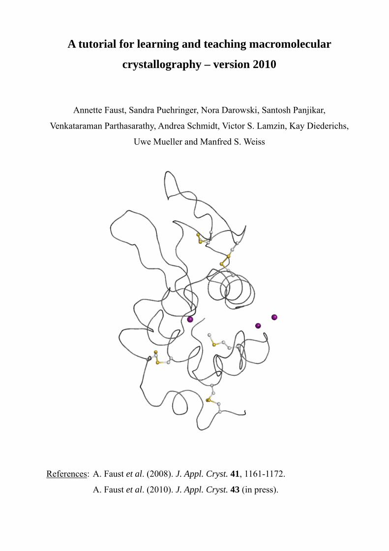
A tutorial for learning and teaching macromolecular

crystallography – version 2010

Annette Faust, Sandra Puehringer, Nora Darowski, Santosh Panjikar,

Venkataraman Parthasarathy, Andrea Schmidt, Victor S. Lamzin, Kay Diederichs,

Uwe Mueller and Manfred S. Weiss

References: A. Faust et al. (2008). J. Appl. Cryst. 41, 1161-1172.

A. Faust et al. (2010). J. Appl. Cryst. 43 (in press).

Experiment 6: Single Isomorphous Replacement with

Anomalous Scattering (SIRAS) on tetragonal lysozyme

Lysozyme is a 129 amino acid enzyme that dissolves bacterial cell walls by catalyzing the

hydrolysis of 1,4-β-linkages between N-acetylmuramic acid and N-acetyl-D-glucosamine

residues in the peptidoglycan layer and between N-acetyl-D-glucosamine residues in

chitodextrins. It is abundant in a number of secreted fluids, such as tears, saliva and mucus.

Lysozyme is also present in cytoplasmic granules of the polymorphonuclear neutrophils (Voet et

al., 2006). Large amounts of lysozyme can also be found for instance in egg whites. The crystal

structure of hen egg-white lysozyme (HEWL) based on crystals belonging to the tetragonal space

group P43212, was the first enzyme structure published (Blake et al., 1965). Over the years,

HEWL has been crystallized in many different crystal forms (for an overview see Brinkmann et

al., 2006) and has become a standard object for methods developments but also for teaching

purposes.

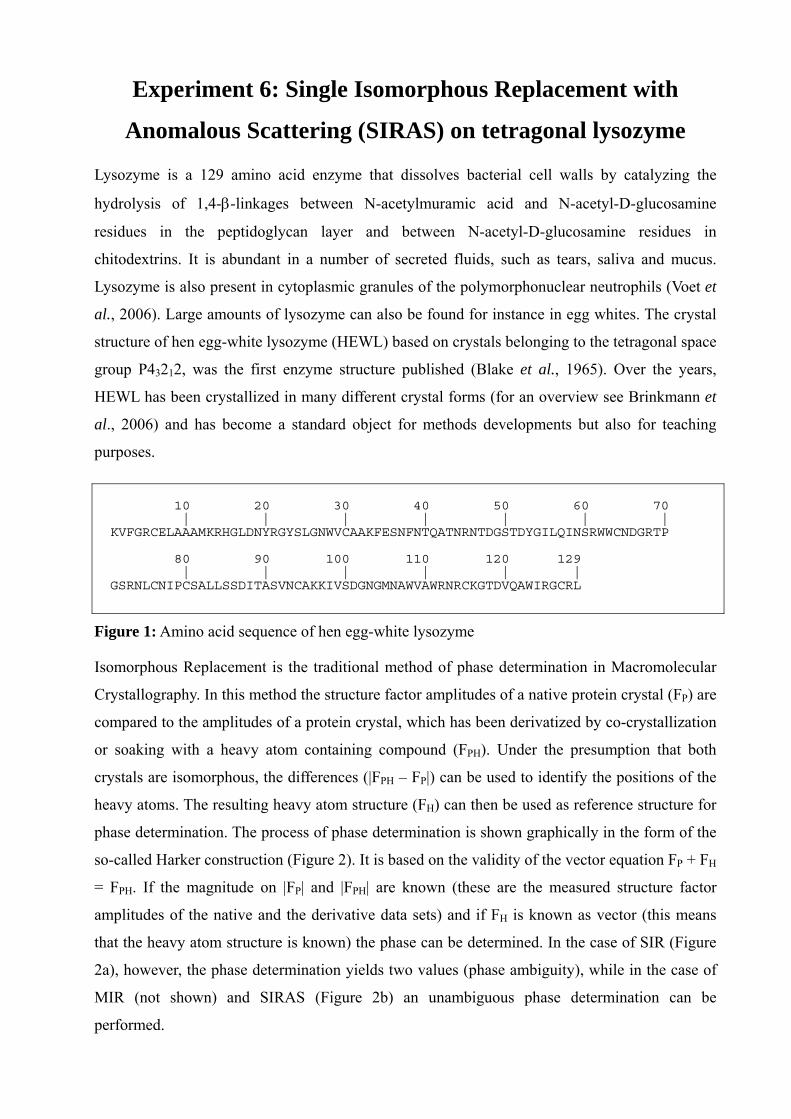
10 20 30 40 50 60 70 | | | | | | |

KVFGRCELAAAMKRHGLDNYRGYSLGNWVCAAKFESNFNTQATNRNTDGSTDYGILQINSRWWCNDGRTP 80 90 100 110 120 129 | | | | | | GSRNLCNIPCSALLSSDITASVNCAKKIVSDGNGMNAWVAWRNRCKGTDVQAWIRGCRL

Figure 1: Amino acid sequence of hen egg-white lysozyme

Isomorphous Replacement is the traditional method of phase determination in Macromolecular

Crystallography. In this method the structure factor amplitudes of a native protein crystal (FP) are

compared to the amplitudes of a protein crystal, which has been derivatized by co-crystallization

or soaking with a heavy atom containing compound (FPH). Under the presumption that both

crystals are isomorphous, the differences (|FPH – FP|) can be used to identify the positions of the

heavy atoms. The resulting heavy atom structure (FH) can then be used as reference structure for

phase determination. The process of phase determination is shown graphically in the form of the

so-called Harker construction (Figure 2). It is based on the validity of the vector equation FP + FH

= FPH. If the magnitude on |FP| and |FPH| are known (these are the measured structure factor

amplitudes of the native and the derivative data sets) and if FH is known as vector (this means

that the heavy atom structure is known) the phase can be determined. In the case of SIR (Figure

2a), however, the phase determination yields two values (phase ambiguity), while in the case of

MIR (not shown) and SIRAS (Figure 2b) an unambiguous phase determination can be

performed.

Figure 2: Harker construction. (a) SIR-case (b) SIRAS -case

1 Crystallisation and Derivatisation

Chemicals: Hen egg-white lysozyme (M ≈ 14600 g/mol, Fluka cat. no. 62970)

CH3COONa (M = 82.03 g/mol, Sigma cat. no. S2889)

CH3COOH (M = 60.0 g/mol, Sigma cat. no. 537020)

NaCl (M = 58.44 g/mol, Sigma cat. no. S7653)

Ethylene glycol (M = 62.07 g/mol, Merck, cat. no. 109621)

KAuCl4 (M = 377.88 g/mol, Aldrich, cat. no. 33,454-5)

Milli-Q water

Tetragonal crystals of HEWL were grown as described by Weiss et al. (2000) by mixing 4 µl of

protein solution (30 mg/ml in water) and 4 µl of reservoir solution containing 50 mM Na acetate

pH 4.5 and 5% (w/v) NaCl and equilibrating the drop against the reservoir. The crystals belong

to space group P43212 (space group number 96) and exhibit the usual unit-cell parameters of a =

78.8 Å and c = 37.2 Å (Figure 3). They appeared within few days after setting up the experiment.

Prior to flash cooling to 100 K, they were transferred into a solution containing 25% (v/v)

ethylene glycol, 10% (w/v) NaCl and 100 mM Na acetate pH 4.5. They typically diffracted X-

rays to a resolution better than 1.6 Å.

300µm

300µm

Figure 3: Tetragonal HEWL crystals.

A 10 mM solution of KAuCl4 in reservoir solution was freshly prepared and one crystal was

soaked in this solution for 1 minute (Sun et al., 2002). This crystal was then also cryo-protected

in a solution containing 25% (v/v) ethylene glycol, 10% (w/v) NaCl and 100 mM Na acetate pH

4.5. The diffraction properties of such derivatized crystals are significantly worse than the ones

for the native crystals but still very much acceptable (Figure 4).

2 Data Collection

Native and derivative X-ray diffraction data have been collected at the tunable beam line BL14.2

at the BESSY-II synchrotron in Berlin-Adlershof. The beam line is equipped with a MARMosaic

CCD detector (225mm) from the company MARRESEARCH (Norderstedt, Germany) and a

MARdtb goniostat (MARRESEARCH, Norderstedt, Germany).

The relevant data collection parameters are given below:

Native Derivative

wavelength 1.00 Å 1.00 Å

detector distance: 180 mm 180 mm

oscillation range/image: 1.0º 1.0º

no. of images: 180 180

exposure time/image: 2.5 sec 5.0 sec

path to images: /exp6/data/native/ /exp6/data/derive/

image names: exp6_lyso_siras_native_###.img

exp6_lyso_siras_deriv_###.img

For the derivative data set, the data collection was interrupted after image 113 due to an

injection. Afterwards, the data collection was continued with the same exposure time but a beam

attenuation using 0.19 mm Al in order to compensate for the increased beam intensity.

Figure 4: Diffraction images of native and derivatized tetragonal lysozyme crystals. The

resolution rings shown are at 7.2, 3.6, 2.4 and 1.8 Å, respectively.

3 Data Processing

The collected diffraction data were indexed, integrated and scaled using the program XDS

(Kabsch, 1993, 2010a,b). XDS is simply run by the command xds. If a multi-processor machine

is available, the command xds_par can be used, which calls a parallel version of XDS and

consequently runs much faster. XDS needs only one input file, which must be called XDS.INP.

No other name is recognized by the program. The file XDS.INP contains all relevant information

about the data collection, from beam parameters to detector parameters and crystal parameters (if

known) as well as the data collection geometry. In XDS.INP one can also define the steps

through which the program should go. This is done by using the parameter JOBS. The following

command, which is equivalent to JOBS= ALL would make XDS run through all eight steps

XYCORR, INIT, COLSPOT, IDXREF, DEFPIX, XPLAN, INTEGRATE and CORRECT.

JOBS= XYCORR INIT COLSPOT IDXREF DEFPIX XPLAN INTEGRATE CORRECT

In the XYCORR step, tables of spatial correction factors are set up (if required). INIT calculates

the gain of the detector and produces an initial background table. COLSPOT identifies strong

reflections which are used for indexing. IDXREF performs the actual indexing of the crystal.

DEFPIX identifies the regions on the detector surface which are used for measuring intensities,

XPLAN helps to devise a data collection strategy, INTEGRATE integrates the reflection

intensities of the whole data set and CORRECT scales and merges symmetry-related reflections

and multiple measurements. It also prints out data processing statistics. After completing each

individual step, a log-file with a name corresponding to the step (STEP-name.LP) is written.

Action 1: edit the supplied file XDS.INP and insert the relevant information about the data

collection, namely the data collection wavelength, crystal-to-detector distance, the direct beam

coordinates, the total number of images, and rotation increment per image and of course very

importantly the path to and the names of the image files. XDS is able to recognize compressed

images; therefore it is not necessary to unzip the data before using XDS. The image name given

must not include the zipping-format extension (*.img instead of *.img.bz2). Further, XDS has a

very limited string length (80) to describe the path to the images. Therefore it may be necessary

to create a soft link to the directory containing the images by using the command ln -s

/path/to/images/ ./images. The path to the images in XDS.INP will then be ./images/. If the space

group and cell dimensions are known, the relevant information should be written into XDS.INP,

if they are not known just set the parameter SPACE GROUP NUMBER= 0.

Action 2: run XDS until the indexing step, with the parameter JOBS set to:

JOBS= XYCORR INIT COLSPOT IDXREF

The output file IDXREF.LP contains the results of the indexing. It needs to be checked carefully

whether the indexing is correct, since all subsequent steps assume the correctness of the indexing

step. The most relevant parameters to look for are the STANDARD DEVIATION OF SPOT

POSITION and the STANDARD DEVIATION OF SPINDLE POSITION. The first one should

be in the order of 1 pixel, whereas the second one depends to some extent on the rotation

increment per image but also on the mosaicity of the crystal. If it is 0.1º it is very good, if it is

0.5º it might still be ok, if it is larger than 1.0º the indexing has probably not worked. The table

with the entries SUBTREE and POPULATION is also very interesting to look at. The first

SUBTREE should have by a large margin more entries than all others. Also, the input

parameters, such as the crystal-to-detector distance should after refinement not deviate too much

from the input values.

The most common problem with the IDXREF step is that it often finishes with the message

!!! ERROR !!! INSUFFICIENT PERCENTAGE (<70%) OF INDEXED REFLECTIONS.

This means that less than 70% of the reflections that were collected in the COLSPOT step are

not indexed, which may happen because of ice rings on the frames, split reflections or simply

wrong input parameters. However, if all indicators of correct indexing are fine (see above) and

no obvious errors can be identified then this message can be safely ignored and data processing

can be continued.

If IDXREF was run with SPACE_GROUP_NUMBER= 0, an assumption of the correct Bravais

lattice may be made at this stage. As a rule of thumb, choose the lattice of the highest possible

symmetry, with a QUALITY OF FIT-value as low as possible (usually < 10). These numbers are

printed in IDXREF.LP in the paragraph DETERMINATION OF LATTICE CHARACTER AND

BRAVAIS LATTICE. Then, re-run the IDXREF step with the parameter

SPACE_GROUP_NUMBER corresponding to the assumed Bravais lattice in XDS.INP.

Alternatively, it is possible to make no assumption of the Bravais lattice at this point, and to

simply continue with data integration. In this case the program will assume that space group

determination should not be based on the metric symmetry of the lattice, but should be

postponed to the CORRECT step (see below).

Nevertheless, if the true lattice is known, it should yield a good, i.e. low QUALITY OF FIT-

number. For tetragonal HEWL, the correct space group is P43212 (space group number 96) with

unit cell parameters of a=78.7 and c=37.1 Å.

Action 3: After the determination of the Bravais lattice and the cell parameters all images need

to be integrated and corrections (radiation damage, absorption, detector etc.) will have to be

calculated. This can be done in a further XDS run.

JOBS= DEFPIX XPLAN INTEGRATE CORRECT

The CORRECT step produces a file called CORRECT.LP, which contains the statistics for the

complete data set after integration and corrections. For the statistics to be meaningful, the correct

Laue symmetry has to be established first. To this end, the CORRECT step compares the

statistics in all possible Laue groups. The correct Laue group is the one with the highest

symmetry, which at the same time still exhibits an acceptable Rr.i.m./Rmeas. CORRECT writes a

file named XDS_ASCII.HKL, which contains the integrated and scaled reflections.

The CORRECT step also performs a refinement of all geometric parameters and the cell

dimensions based on all reflections of the data set. These parameters may be more accurate than

the ones obtained from the indexing step. Therefore, one may try to use the refined parameters

and to re-run the last XDS job. In order to not overwrite the original results, it is advisable to

save all current files to a temporary directory. Then, the file GXPARM.XDS should be renamed

or copied to XPARM.XDS and XDS be re-run. In case the original results are better, they can be

copied back to the original directory.

While XDS will usually identify the correct Laue group, it does not determine the actual space

group of the crystal. The decision about the existence of screw axes is left to the user.

Indications, which screw axes may be present can be obtained from the table REFLECTIONS

OF TYPE H,0,0 0,K,0 0,0,L OR EXPECTED TO BE ABSENT (*) in the file CORRECT.LP.

Alternatively, the program POINTLESS (Evans 2005) offers an automatic way of assigning the

space group. POINTLESS can be run with the command pointless XDSIN XDS_ASCII.HKL. In

the output the possible space groups together with their probabilities are given. Some space

group ambiguity still remains at this stage, since it is impossible to distinguish between

enantiomorphic space groups e.g. P31 and P32, or P41212 and P43212 just based on intensities.

This ambiguity has to be resolved later during structure solution. The parameter

SPACE_GROUP_NUMBER corresponding to the determined space group as well as the cell

parameters should be entered into the file XDS.INP for running the next step.

Action 4: Finally, outlier reflections are identified by CORRECT by comparing their intensity to

the average intensity in their respective resolution shells. These outliers may be removed, if there

is a clear indication and reason for their existence: for example, ice rings often produce very

strong reflections at specific d-spacings. The outliers are flagged as ‘alien’ in the file

CORRECT.LP and their removal can simply be achieved by writing the outliers into a file called

REMOVE.HKL. By re-running XDS with the command

JOBS= CORRECT

in XDS.INP, these outliers are then disregarded. This last action can be repeated until no more

additional outliers are identified. However, the outlier removal has to be handled very carefully

because strong reflections may also arise from non-crystallographic symmetry and in particular

from the presence of pseudo-translation. A command to identify only the most extreme outliers

would be awk '/alien/ { if (strtonum($5) > 19) print $0 }' CORRECT.LP >> REMOVE.HKL.

This command will remove outliers only when their Z-score is above 19. Hints to suitable

criteria for outlier rejection can be found in the XDSwiki (http://strucbio.biologie.uni-

konstanz.de/xdswiki), where this question is treated specifically in the article “Optimization”.

Action 5:, The CORRECT step can be followed up by running the scaling program XSCALE,

which is part of the XDS program package. This serves three purposes: a) the user may specify

the limits of the resolution shells for which statistics should be printed, b) several

XDS_ASCII.HKL files may be scaled together and c) correction factors for radiation damage

may be applied to the data (see also the article “XSCALE” in the XDSwiki). XSCALE is run by

simply typing xscale (or xscale_par to speed up the computation on a multi-processor machine)

provided that a file XSCALE. INP defining the input and output files is present. As above in the

CORRECT step, outliers may be rejected. XSCALE writes out a *.ahkl file, which can be

converted with XDSCONV to be used within the CCP4-suite (Collaborative Computational

Project, 1994) or other programs.

Both CORRECT and XSCALE will produce all necessary output for assembling a table with all

relevant data processing statistics, which is necessary for a publication.

Table 1: Data processing statistics (in this case from CORRECT.LP)

Native Derivative

Resolution limits [Å] 50.0 - 1.60 (1.70 - 1.60) 50.0 - 1.80 (1.91 - 1.80)

Space group P43212 P43212

Unit cell parameters a, c [Å] 78.62, 36.81 78.73, 36.73

Mosaicity [˚] 0.13 0.17

Total number of reflections 187497 152422

Unique reflections 28363 20439

Redundancy 6.6 (3.4) 7.5 (7.1)

Completeness [%] 97.4 (86.3) 99.5 (97.5)

I/σ(I) 27.4 (5.2) 15.6 (3.0)

Rr.i.m. / Rmeas [%] 4.8 (24.6) 9.9 (71.1)

Wilson B-factor [Å2] 20.3 28.3

Action 6: finally, the processed intensity file needs to be converted to certain file formats, which

are used by other programs to perform the necessary structure determination steps. This can be

achieved using the program XDSCONV, which can simply be run by using the command

xdsconv provided that a file called XDSCONV.INP is present. XDSCONV.INP just needs to

contain information about the name of the input file and about the name and type of the output

file. If a CCP4-type file is required, XDSCONV reformats the reflection output file from

XSCALE and creates an input file F2MTZ.INP for the final conversion of the reflection file to

binary mtz-format, which is the standard format for all CCP4 programs (CCP4, 1994).

OUTPUT_FILE=lyso_siras.hkl CCP4

INPUT_FILE=lyso_siras.ahkl

To run the CCP4 programs F2MTZ and CAD, just type the two commands

f2mtz HKLOUT temp.mtz < F2MTZ.INP

and

cad HKLIN1 temp.mtz HKLOUT lyso_siras_ccp4.mtz << eof

LABIN FILE 1 ALL

END

eof

Some CCP4 programs need the intensities of the Bijvoet pairs as input. For those the second

parameter on the OUTPUT_FILE= line should be CCP4_I instead of CCP4. Alternatively, the

file XDS_ASCII.HKL can be converted to mtz-format using the CCP4-programs COMBAT or

POINTLESS (Evans, 2005) and this mtz-file can be used as an input file for the scaling program

SCALA (Evans, 2005) in CCP4. More information on this can be found in the articles

“Pointless” and “Scaling with SCALA” in the XDSwiki.

With an R-factor to the native data set of 22% and an anomalous correlation coefficient CCanom

of 47% (calculated using the CCP4 program SCALEIT), the derivative data set contains

significant isomorphous and anomalous signal, respectively. This is exemplified by the

inspection of Patterson maps (Figure 5), which have been calculated based on the isomorphous

differences (|FPH| - |FP|) or the anomalous differences (|FPH+| - |FPH-|) using the program FFT

within the CCP4-suite.

(a) (b)

Figure 5: Difference (a) and anomalous difference (b) Patterson map. Shown are the Harker

sections w=1/4 in both cases. The peak denoted AA and the corresponding symmetry related

peaks are the Harker peaks of the Au site no. 1.

4 Structure Solution

The structure can be solved using the SIRAS-protocol (advanced version) of Auto-Rickshaw, the

EMBL-Hamburg automated crystal structure determination platform (Panjikar et al., 2005,

2009). AUTO-RICKSHAW can be accessed from outside EMBL under www.embl-

hamburg.de/Auto-Rickshaw/LICENSE (a free registration may be required, please follow the

instructions on the web page). In the following the automatically generated summary of AUTO-

RICKSHAW is printed together with the results of the structure determination:

The input diffraction data files XDS_ASCII.HKL were uploaded and then prepared and

converted using programs of the CCP4-suite (CCP4, 1994). ∆F and | |FPH-| - |FP| |-values were

calculated using the program SHELXC (Sheldrick et al., 2001, Sheldrick, 2008). Based on an

initial analysis of the data, the maximum resolution for substructure determination and initial

phase calculation was set to 2.4 A. Three heavy atom sites were found using the program

SHELXD (Schneider & Sheldrick, 2002) with correlation coefficients of 35.98% and 23.74% for

all and for just the weak reflections, respectively. The correct hand for the substructure was

determined using the programs ABS (Hao, 2004) and SHELXE (Sheldrick, 2002). Initial phases

were calculated after density modification using the program SHELXE. A poly-Ala model was

automatically built using the program SHELXE and ARP/wARP (Perrakis et al., 1999; Morris et

al., 2004). This resulted in a model, which was 95% complete already. To complete the model

and to enhance the phases the MRSAD module of AUTO-RICKSHAW (Panjikar et al., 2009)

was used. This resulted in a model consisting of 127 residues, of which 125 were docked in the

amino acid sequence. This model was refined using REFMAC5 and further modified using

COOT (Emsley, 2004). The final R-factor for the model was 21.8% and the free R-factor was

27% (see directory exp6/struct_ref/).

Table 2: List of heavy atom peaks found using SHELXD corresponding to the three Au sites.

Rank x y z Occupancy

1 67.093 11.725 0.909 1.00

2 69.980 9.972 -4.114 0.69

3 67.297 11.323 -9.203 0.33

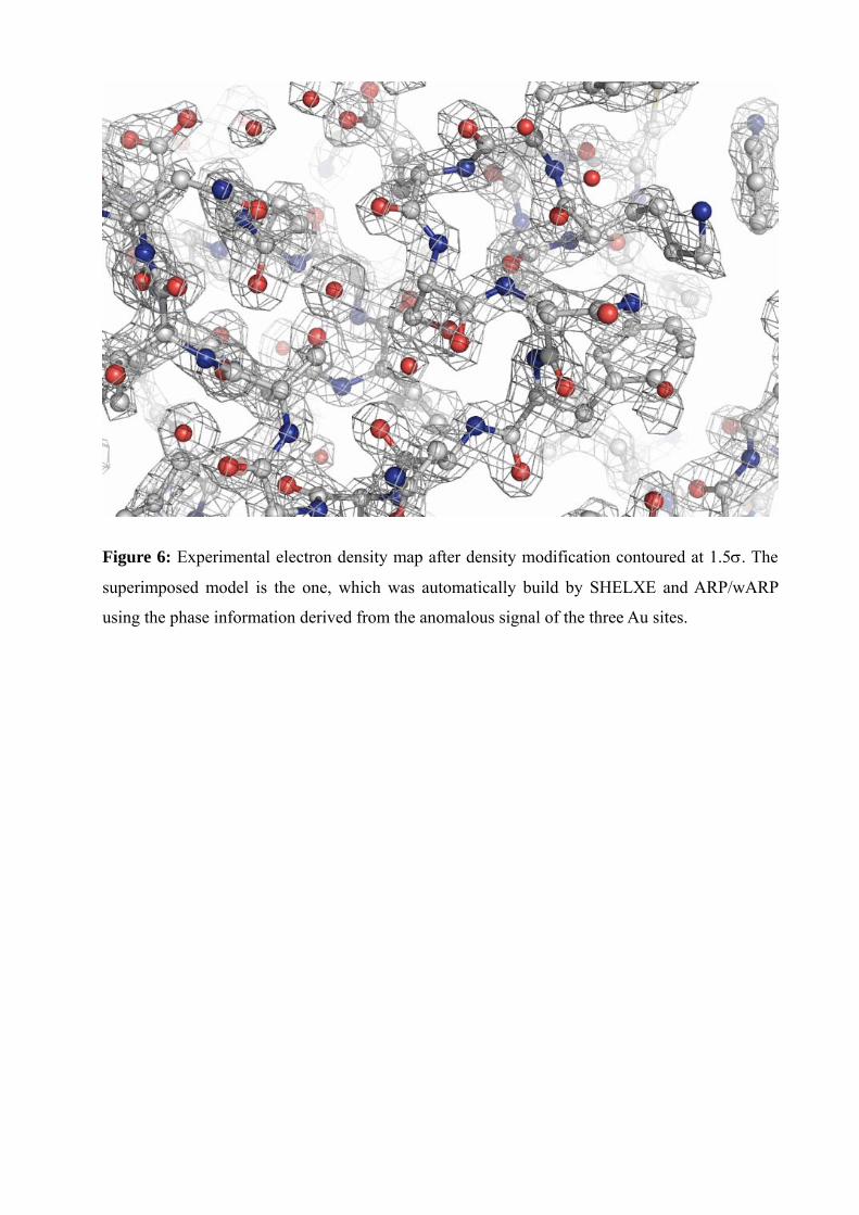
Figure 6: Experimental electron density map after density modification contoured at 1.5σ. The

superimposed model is the one, which was automatically build by SHELXE and ARP/wARP

using the phase information derived from the anomalous signal of the three Au sites.

Figure 7: Refined structure of the KAuCl4-derivative of tetragonal HEWL presented as a thin

tube (in gray). Also shown are the Met and Cys side chains of HEWL (as ball-and-stick) and the

bound gold atoms (in purple). Superimposed on the structure is the anomalous difference Fourier

electron density map contoured at 4.0 σ. The first Au-atom is located 3.6 Å from the SD-atom of

Met105 and 4.4 Å from the NE-atom of Trp108. The second and the third Au atoms are located

on both sides of the side chain of His15. One is located 2.1 Å from the NE2-atom while the other

is found 2.0 Å from the ND1-atom of His15.

5 References

Blake, C. C. F., Koenig, D. F., Mair, G. A., North, A. C. T., Philipps, D. C. & Sarma, V. R.

(1965). Nature 206, 757-761.

Brinkmann, C., Weiss, M. S. & Weckert, E. (2006). Acta Cryst. D62, 349-355.

Collaborative Computational Project, Number 4 (1994). Acta Cryst. D50, 760-763.

Emsley, P. & Cowtan, K. (2004). Acta Cryst. D60, 2126-2132.

Evans, P. (2005). Acta Cryst. D62, 72-82.

Hao, Q. (2004). J. Appl. Cryst. 37, 498-499.

Kabsch, W. (1993). J. Appl. Cryst. 26. 795-800.

Kabsch, W. (2010a). Acta Cryst. D66, 125-132.

Kabsch, W. (2010b). Acta Cryst. D66, 133-144.

Morris, R. J., Perrakis, A. & Lamzin, V.S. (2002). Acta Cryst. D58, 968-975.

Murshudov, G. N., Vagin, A. A. & Dodson, E. J. (1997). Acta Cryst. D53, 240-255.

Panjikar, S., Parthasarathy, V., Lamzin, V. S., Weiss, M. S. & Tucker, P. A. (2005). Acta Cryst.

D61, 449-457.

Panjikar, S., Parthasarathy, V., Lamzin, V. S., Weiss, M. S. & Tucker, P. A. (2009). Acta Cryst.

D65, 1089-1097.

Perrakis, A., Morris, R. J. & Lamzin, V. S. (1999). Nature Struct. Biol. 6, 458-463.

Schneider, T. R. & Sheldrick, G. M. (2002). Acta Cryst. D58, 1772-1779.

Sheldrick, G. M., Hauptman, H. A., Weeks, C. M., Miller, R. & Uson, I. (2001). International

Tables for Macromolecular Crystallography, Vol. F, edited by M. G. Rossmann & E. Arnold,

ch. 16, pp. 333-345. Dordrecht: Kluwer Academic Publishers.

Sheldrick, G. M. (2002). Z. Kristallogr. 217, 644-650.

Sheldrick, G. M. (2008). Acta Cryst. A64, 112-122.

Sun, P. D., Radaev, S. & Kattah, M. (2002). Acta Cryst, D58, 1092-1098.

Terwilliger, T. C. (2000). Acta Cryst. D56, 965-972.

Voet, D., Voet, J. & Pratt, C. W. (2006). Fundamentals in Biochemistry - Life at the molecular

level, 2nd Edition, John Wiley & Sons, Inc., Hoboken, NJ, USA.

Weiss, M. S., Palm, G. J. & Hilgenfeld, R. (2000). Acta Cryst. D56, 952-958.