Boundary-Layer Meteorologyhttps://doi.org/10.1007/s10546-019-00495-8

RESEARCH ART ICLE

A Turbulence Closure Study of the Flow and Thermal Fields inthe Ekman Layer

Lukas Braun1 · Bassam A. Younis2 · Bernhard Weigand1

Received: 19 April 2019 / Accepted: 30 November 2019© Springer Nature B.V. 2019

AbstractWe assess the performance of turbulence closures of varying degrees of sophistication in theprediction of the mean flow and the thermal fields in a neutrally-stratified Ekman layer. TheReynolds stresses that appear in the Reynolds-averagedmomentum equations are determinedusing both eddy-viscosity and complete differential Reynolds-stress-transport closures. Theresults unexpectedly show that the assumption of an isotropic eddy viscosity inherent ineddy-viscosity closures does not preclude the attainment of accurate predictions in this flow.Regarding the Reynolds-stress transport closure, two alternative strategies are examined:one in which a high turbulence–Reynolds–number model is used in conjunction with awall function to bridge over the viscous sublayer and the other in which a low turbulence–Reynolds-number model is used to carry out the computations through this layer directly tothe surface. It is found that the wall-function approach, based on the assumption of the appli-cability of the universal logarithmic law-of-the-wall, yields predictions that are on par withthe computationally more demanding alternative. Regarding the thermal field, the unknownturbulent heat fluxes are modelled (i) using the conventional Fourier’s law with a constantturbulent Prandtl number of 0.85, (ii) by using an alternative algebraic closure that includesdependence on the gradients of mean velocities and on rotation, and (iii) by using a differ-ential scalar-flux transport model. The outcome of these computations does not support theuse of Fourier’s law in this flow.

Keywords Ekman layer · Prandtl number · Reynolds-stress closures · Similarity theory ·Turbulent heat-flux closures

1 Introduction

Most turbulence closures in use for the prediction of environmental flows in general, and theatmospheric boundary layer (ABL) in particular, have been developed and calibrated with

B Bassam A. Younisbayounis@ucdavis.edu

1 Institut für Thermodynamik der Luft- und Raumfahrt, Universität Stuttgart, Stuttgart, Germany

2 Department of Civil and Environmental Engineering, University of California - Davis, Davis, CA95616, USA

123

L. Braun et al.

reference to experimental data from simple, uni-directional two-dimensional shear flowsin which complicating effects such as those arising from buoyancy, streamline curvature,or system rotation are entirely absent. In the Ekman layer–the boundary layer formed bypressure gradients induced in a rotating system and which is considered to be a realisticsimpler representation of the ABL–the flow is three dimensional, the direction of the resultantvelocity varies with height (the Ekman spiral) and, further, rotational effects appear explicitlyin the equations governing the transport of momentum, and in the transport equations forthe turbulent fluxes of momentum, heat, and contaminants. Thus some of the modellingassumptions inherent in these closures may no longer be valid in this more complex flow.One such assumption that is central to conventional turbulence closures, but whose validityin the more general ABL flow may be questionable, is that of Boussinesq in which theunknown Reynolds stresses are assumed to be proportional to the local mean rates of strainimplying alignment of their respective directions. For this to be the case, the contributionsof the convective and diffusive transport processes to the balances of the Reynolds stressesmust be negligible compared to the processes of generation and dissipation. However, thiscondition is not always obtained (Kannepalli and Piomelli 2000). Moreover, in practicalapplications, the coefficient of proportionality, the eddy viscosity, is assumed to be isotropicwhen in fact measurements of three-dimensional shear flows show that this is not generallythe case (Johnstone and Flack 1996). There is therefore a need to carefully evaluate theperformance in the Ekman layer of some of the more commonly-used closures using reliableresults obtained in recent direct numerical simulations (DNS) and experiments.

A number of studies on the assessment of turbulence closures for the Ekman layerhave been reported in the literature. We confine attention here to those that used the morephysically-based and widely-used 1.5- and 2.5-order turbulence closures. Of the former cat-egory, the k−ε model, with k being the turbulence kinetic energy (TKE) and ε its dissipationrate, appears to have received the most attention. Detering and Etling (1985), Andrén (1991),and Apsley and Castro (1997) found it necessary when using this model to modify the pro-duction term in the ε equation to improve the prediction of the wind profile in the ABL. Inall these studies, the eddy viscosity was assumed to be isotropic. In contrast, Wirth (2010)postulated that the eddy viscosity is an anisotropic fourth-order tensor in three-dimensionalspace and derived an expression for it that produced good results for the Ekman spiral. Mar-latt et al. (2012) used their DNS results to evaluate this model. They found that the closestagreement between the k−ε model results and the DNS data is obtained when the coefficientCμ that enters into the calculation of the eddy viscosity is made a function of the turbulentReynolds number. This coefficient was taken as constant in the previous studies, a practicethat Marlatt et al. (2012) found to produce the least satisfactory agreement with the DNSresults. We include the k − ε model in our assessment.

The notion of turbulent viscosity is dispensedwithin 2.5-order turbulence closureswhereinthe Reynolds stresses are obtained from the solution of a modelled differential transportequation for each component, a total of six for the Ekman layer. In this study, we evaluatetwo models of this category. These models have in common several of the approximationsneeded to close the exact equations for the Reynolds stresses but differ in one importantrespect: one is applicable only in the fully-turbulent region of the flow, thereby requiring theassumption that the universal logarithmic law-of-the-wall is valid so it can be used to bridgeover the viscous sublayer, and another that is also applicable in the viscous sublayer therebyallowing for the simulations to be extended directly to the wall. Apart from determining theinfluence of each approach on the quality of the predictions, the results obtained with thesemodels serve to show the extent to which the effects of convective and diffusive transport areimportant in such a flow. Furthermore, because all three models are solved using the same

123

A Turbulence Closures Study of the Flow and Thermal…

computational tool, and their results tested against the same benchmark data, differences intheir results can be attributed to their formulation with greater certainty.

We also consider the question of how best to model the turbulent transport of heat in theneutral Ekman layer, a topic that, despite its obvious importance, has received relatively lessattention than that of the flow field. The usual approach to modelling the turbulent heat fluxesis to assume them to be proportional to the local gradients of mean potential temperature.The proportionality coefficient, the turbulent diffusivity, is in turn taken to be proportionalto the turbulent viscosity via a turbulent Prandtl number typically taken to be constant. Theassumption of a constant turbulent Prandtl number has been the subject of numerous studies,most recently by Li (2019) who found no evidence to support it. Here, we use this approachtomodelling the heat fluxes and compare this with two other models that are entirely differentin their formulation: one that is also algebraic in the heat fluxes but allows for the turbulentPrandtl number to vary depending on the details of the turbulence field, and another inwhich the fluxes are obtained from the solution of modelled differential transport equation,a total of three in the Ekman layer. The objective of these simulations is to place on recordthe performance of these three different modelling approaches and thus provide a basis forassessing their suitability for use in this flow.

While many of the features that pose the Ekman layer as an exacting test for turbulenceclosures are considered,we note thatABLflows are subject to complicating effects that are notconsidered here but whose presence can adversely affect the performance of these closures.Three complicating effects are worthy of note, these are: stable stratification, mean-flowunsteadiness and surface drag effects. The effects of stable stratification are to diminish theturbulence activity leading to reduction in the vertical turbulent fluxes of heat andmomentumrelative to the neutrally-stratified flow. A number of alternative approaches to sensitizing theturbulence closures to the effects of stable stratification have been proposed. Mauritsen et al.(2007), for example, proposed a model in which the TKE k, which is typically used ineddy-viscosity closures to obtain a characteristic turbulent velocity scale, is replaced by thetotal turbulence energy being the sum of k and the turbulent potential energy. The model’sperformance was assessed by comparisons with large-eddy simulations (LES) for neutral andstably-stratified cases where it was found to yield results that were indistinguishable fromthose of LES. Concerning the effects of mean-flow unsteadiness on the Ekman layer, large-eddy simulations by Momen and Bou-Zeid (2017) of a neutral flow with unsteady pressureforcing indicated that these effects are determined by the relative magnitudes of the timescales for the inertial and turbulence processes, and the pressure forcing. The results wereused to test first- and 1.5-order turbulence closures which, for the case where the forcingand the turbulence time scales are comparable, were found to fail badly in capturing thechanges wrought on the flow dynamics by virtue of the turbulence being out of equilibriumwith the mean flow. The matter of how to account, in a turbulence closure, for the effects ofsurface drag produced by tall vegetative canopies was considered by Sogachev et al. (2012)who advanced a model based on extension of the equation for the turbulence length scale.The model proved successful in reproducing the effects of both vegetation and atmosphericstability. Consideration of howbest to account for these complicating effects in the frameworkof the turbulence closures that are the focus of the present contribution is deferred to a futurestudy.

123

L. Braun et al.

2 Mathematical Formulation

2.1 Mean-Flow Equations

The coordinate system used is shown in Fig. 1, where the x- and y-axes are the horizontalcoordinates and z is the vertical coordinate. The x-component of the freestream geostrophicvelocity vector is Ug = (Ug, 0).

The flow is assumed to be horizontally homogeneous and hence all gradients in the y-direction vanish, and in accordance with the usual boundary-layer assumptions, diffusion isconsidered to be important only in the vertical direction. The flow is taken to be steady and thefluid (air) to be of constant properties. With these assumptions, the time-averaged equationsgoverning the conservation of mass, momentum, and thermal energy (temperature) can bewritten as

∂U

∂x+ ∂W

∂z= 0, (1)

U∂U

∂x+ W

∂U

∂z= ∂

∂z

(ν∂U

∂z− uw

)− 1

ρ

∂ p

∂x+ f V , (2)

U∂V

∂x+ W

∂V

∂z= ∂

∂z

(ν∂V

∂z− vw

)− 1

ρ

∂ p

∂ y− f U , (3)

U∂�

∂x+ W

∂�

∂z= ∂

∂z

(ν

Pr

∂�

∂z− wθ

). (4)

In the above, U , V , and W are the velocity components in the x-, y-, and z-directionsrespectively, p is the time-averaged static pressure, � is the potential temperature, Pr is themolecular Prandtl number, ρ is the density, ν is the kinematic viscosity, and f is the Coriolisfrequency,

f = 2�sin(φ), (5)

Fig. 1 Geostrophic coordinatesystem and a visualization of thecomputed Ekman spiral at 90◦ N

123

A Turbulence Closures Study of the Flow and Thermal…

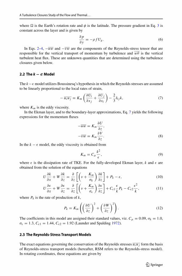
where � is the Earth’s rotation rate and φ is the latitude. The pressure gradient in Eq. 3 isconstant across the layer and is given by

∂ p

∂ y= −ρ f Ug. (6)

In Eqs. 2–4, −uw and −vw are the components of the Reynolds-stress tensor that areresponsible for the vertical transport of momentum by turbulence and wθ is the verticalturbulent heat flux. These are unknown quantities that are determined using the turbulenceclosures given below.

2.2 The k− �Model

The k−ε model utilizes Boussinesq’s hypothesis in which the Reynolds stresses are assumedto be linearly proportional to the local rates of strain,

− uiu j = Km

(∂Ui

∂x j+ ∂Uj

∂xi

)− 2

3δi j k, (7)

where Km is the eddy viscosity.In the Ekman layer, and to the boundary-layer approximations, Eq. 7 yields the following

expressions for the momentum fluxes

−uw = Km∂U

∂z,

−vw = Km∂V

∂z. (8)

In the k − ε model, the eddy viscosity is obtained from

Km = Cμ

k2

ε, (9)

where ε is the dissipation rate of TKE. For the fully-developed Ekman layer, k and ε areobtained from the solution of the equations

U∂k

∂x+ W

∂k

∂z= ∂

∂z

[(ν + Km

σk

)∂k

∂z

]+ Pk − ε, (10)

U∂ε

∂x+ W

∂ε

∂z= ∂

∂z

[(ν + Km

σε

)∂ε

∂z

]+ Cε1

ε

kPk − Cε2

ε2

k, (11)

where Pk is the rate of production of k,

Pk = Km

((∂U

∂z

)2

+(

∂W

∂z

)2)

. (12)

The coefficients in this model are assigned their standard values, viz. Cμ = 0.09, σk = 1.0,σε = 1.3, Cε1 = 1.44, Cε2 = 1.92 (Launder and Spalding 1972).

2.3 The Reynolds-Stress Transport Models

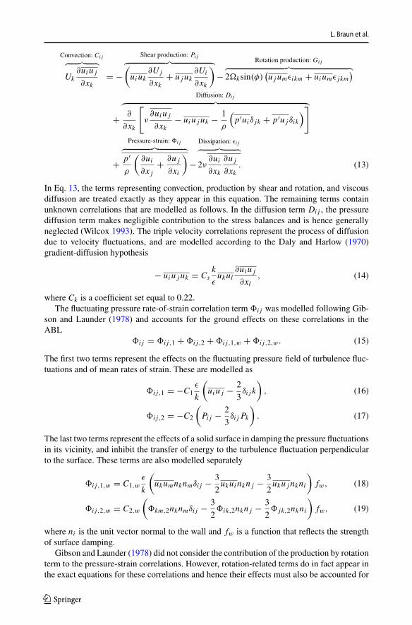
The exact equations governing the conservation of the Reynolds stresses uiu j form the basisof Reynolds-stress transport models (hereafter, RSM refers to the Reynolds-stress model).In rotating coordinates, these equations are given by

123

L. Braun et al.

Convection: Ci j︷ ︸︸ ︷Uk

∂uiu j

∂xk= −

Shear production: Pi j︷ ︸︸ ︷(uiuk

∂Uj

∂xk+ u juk

∂Ui

∂xk

)−

Rotation production: Gi j︷ ︸︸ ︷2�ksin(φ)

(u jumεikm + uiumε jkm

)

+

Diffusion: Di j︷ ︸︸ ︷∂

∂xk

[ν∂uiu j

∂xk− uiu j uk − 1

ρ

(p′uiδ jk + p′u jδik

)]

+

Pressure-strain: �i j︷ ︸︸ ︷p′ρ

(∂ui∂x j

+ ∂u j

∂xi

)−

Dissipation: εi j︷ ︸︸ ︷2ν

∂ui∂xk

∂u j

∂xk. (13)

In Eq. 13, the terms representing convection, production by shear and rotation, and viscousdiffusion are treated exactly as they appear in this equation. The remaining terms containunknown correlations that are modelled as follows. In the diffusion term Di j , the pressurediffusion term makes negligible contribution to the stress balances and is hence generallyneglected (Wilcox 1993). The triple velocity correlations represent the process of diffusiondue to velocity fluctuations, and are modelled according to the Daly and Harlow (1970)gradient-diffusion hypothesis

− uiu j uk = Csk

εukul

∂uiu j

∂xl, (14)

where Ck is a coefficient set equal to 0.22.The fluctuating pressure rate-of-strain correlation term �i j was modelled following Gib-

son and Launder (1978) and accounts for the ground effects on these correlations in theABL

�i j = �i j,1 + �i j,2 + �i j,1,w + �i j,2,w. (15)

The first two terms represent the effects on the fluctuating pressure field of turbulence fluc-tuations and of mean rates of strain. These are modelled as

�i j,1 = −C1ε

k

(uiu j − 2

3δi j k

), (16)

�i j,2 = −C2

(Pi j − 2

3δi j Pk

). (17)

The last two terms represent the effects of a solid surface in damping the pressure fluctuationsin its vicinity, and inhibit the transfer of energy to the turbulence fluctuation perpendicularto the surface. These terms are also modelled separately

�i j,1,w = C1,wε

k

(ukumnknmδi j − 3

2ukui nkn j − 3

2uku j nkni

)fw, (18)

�i j,2,w = C2,w

(�km,2nknmδi j − 3

2�ik,2nkn j − 3

2� jk,2nkni

)fw, (19)

where ni is the unit vector normal to the wall and fw is a function that reflects the strengthof surface damping.

Gibson and Launder (1978) did not consider the contribution of the production by rotationterm to the pressure-strain correlations. However, rotation-related terms do in fact appear inthe exact equations for these correlations and hence their effects must also be accounted for

123

A Turbulence Closures Study of the Flow and Thermal…

in the model for these correlations. Here, we adopt the proposals of Younis et al. (1998) byincorporating the production by rotation term in a manner analogous to Eq. 17

�i j,3 = −C3

(Gi j − 2

3δi j Gii

). (20)

Following Gibson and Launder (1978) and Younis et al. (1998), the coefficients thatappear in Eqs. 14–20 are assigned the values C1 = 1.8, C2 = 0.6, C3 = 0.6, C1,w = 0.5,C2,w = 0.3, Cs = 0.22.

Since the fluid viscosity is absent from the exact equations for the fluctuating triple velocitycorrelations and thepressure-strain correlations, itmay reasonablybe assumed that themodelsfor these correlations, which themselves are independent of viscosity, are valid across theentire range of turbulence Reynolds number. This does not apply to the last term in Eq. 13,which represents the rate atwhich ui u j is dissipated by viscous action.Here,we do expect thatthe model for εi j should reflect the DNS and experimental results that indicate that viscousdissipation is highly anisotropic in the viscosity-affected region of the flow but becomesisotropic in the high turbulent–Reynolds-number regions of the flow away from solid walls.A model that reflects the correct asymptotic behaviour of the dissipation rate term at bothlow- and high-turbulence Reynolds number is given by Kebede et al. (1985)

εi j = ε

[2

3δi j (1 − fs)

+ fs Fuiu j + uiuknkn j + u juknkni + δi j ukulnknl

k

], (21)

where ni is again the unit vector normal to the surface. The function fs in Eq. 21 is a functionof the turbulence Reynolds number Ret

fs = exp(−Ret/40), (22)

with Ret = k2/(νε). Close to thewall, in the viscous sublayer, Ret is low and fs approaches avalue of unity which eliminates the isotropic contribution and produces the correct anisotropyof the dissipation tensor. Farther away from the wall, Ret is high and fs approaches zero,and in this case, the model correctly obtains the expected isotropic dissipation result. Thefunction F in Eq. 21, which is necessary to ensure that the trace of εi j yields the result εi i =2ε, has the form

F =(1 + 5

2

ukulk

nknl

)−1

. (23)

Differences between the high and low-Ret models are also present in the equation fromwhich ε is obtained. This equation can be written in a unified form applicable to both modelsas

Ul∂ε

∂xl= ∂

∂xl

[(νδml + Cε

k

εumul

)∂ε

∂xm

]

+ Cε1ε

kPk − Cε2

εε

k+ Cε3ν

k

εukul

(∂2Ui

∂x j∂xl

)(∂2Ui

∂xk∂xl

). (24)

When Eq. 24 is used for the low-Ret model calculations, it is more convenient from thestandpoint of specifying the boundary conditions at the wall to solve an equation in which ε

123

L. Braun et al.

Table 1 Coefficients of the ε

equationModel Cε Cε1 Cε2 Cε3 Cε4

High Ret 0.18 1.45 1.90 0 0

Low Ret 0.18 1.45 (1 − fs ) + 2.0 fs 1.90 0.3 1.0

is replaced everywhere by ε∗

ε∗ = ε − 2Cε4ν

(∂√k

∂xl

)2

, (25)

where ε∗ is the difference between ε and its value at the wall and can hence be set equal tozero there. The model coefficients are listed in Table 1.

2.4 Algebraic Turbulent Heat-Flux Models

2.4.1 Linear Model

In the linear model for the turbulent heat fluxes (Fourier’s law), the heat fluxes are related tothe local gradients of the potential temperature

− uiθ = Kh∂�

∂xi, (26)

where Kh is the turbulent diffusivity. In the fully-developed horizontally homogeneousEkman layer, Eq. 26 gives the vertical turbulent heat flux as

− wθ = Kh∂�

∂z. (27)

The turbulent diffusivity is typically related to the turbulent viscosity via the turbulent Prandtlnumber (Prt ) i.e.,

Kh = Km

Prt, (28)

where Prt is the turbulent Prandtl number which is typically assumed to be constant. Itsvalue, deduced from laboratory experiments, ranges from 0.73 to 0.92 (Kays 1994). In theABL, the precise value for Prt is the subject of ongoing research (see, for example, therecent review by Li 2019). In our work, we assign to this parameter the constant value of0.85, which represents an average of the experimentally determined values.

It is worth noting here that Fourier’s law aligns the directions of the turbulent heat fluxeswith those of the temperature gradients. Thus in a flow, such as the present, where the onlyfinite temperature gradient is in the z-direction, Eq. 26 indicates that only the vertical turbulentheat flux is finite–the horizontal flux components (uθ and vθ ) being identically zero. Thisfeature of the linear turbulent flux model is of no consequence here since it is restricted tothe case of neutral stratification. This would not be the case in vertical stratified flows (e.g.plumes) since the horizontal fluxes there enter into the expression for the buoyant rate ofgeneration of TKE (Malin and Younis 1990).

123

A Turbulence Closures Study of the Flow and Thermal…

Table 2 Coefficients of thenon-linear algebraic heat fluxmodel

C1t C2t C3t ξ χ

0.03 0.21 0.105 0.2 4.0

2.4.2 Non-Linear Turbulent Flux Model

It will be seen in the next subsection that the exact equations for uiθ require the turbulent heatfluxes to explicitly dependon the gradients ofmeanvelocity andon the rotation rate.Anumberof alternative proposals have been reported in the literature. We use the model proposed byMüller et al. (2015) because it has been extensively tested and because it incorporates anexplicit dependence on the rotation rate. The model equation is

−uiθ = C∗1tk2

ε

∂�

∂xi+ C2t

k

εuiu j

∂�

∂x j

− C3tk2

ε2

[uiuk

(∂Uj

∂xk+ ε jmk�msin(φ)

)

+u juk

(∂Ui

∂xk+ εimk�msin(φ)

)]∂�

∂x j, (29)

with C∗1t given by

C∗1t = C1t

(1 − exp(−Aχ Peξ

t ))

, (30)

where Pet (= Pr Ret ) is the turbulent Peclet number and A is a parameter that depends onthe second and third invariants of the Reynolds-stress anisotropy tensor. The values assignedto the model coefficients are listed in Table 2.

In the Ekman layer, Eq. 29 obtains the vertical heat flux as

− wθ =

Kh︷ ︸︸ ︷k2

ε

(C∗1t + C2t

w2

k

)∂�

∂z. (31)

Note that Fourier’s law with constant turbulent Prandtl number can be recovered from Eq. 31by setting C∗

1 = Cμ/Prt and C2t = 0. On the other hand, by retaining the assigned valuesfor these coefficients, Eq. 31 can be recast in the manner of Eq. 28 with the eddy viscositydefined as in Eq. 9 to yield an expression for a variable turbulent Prandtl number

Prt = Cμ

C∗1t + C2tw2/k

. (32)

Aphysical interpretationmay be attached to Eq. 32: in the Ekman layer, the presence of a solidsurface inhibits the transfer of turbulence energy from the normal-stress components whereit is directly generated into w2, the component perpendicular to the surface. A reduction inthe level of w2 compared to that in a free shear layer leads to a relatively higher value of Prtin the wall-bounded flow. This is consistent with experimental observations (e.g. Launder1976).

123

L. Braun et al.

2.5 Differential Transport Model for the Turbulent Fluxes

The exact equation describing the conservation of the turbulent heat fluxes in rotating coor-dinates is given by (see e.g. Younis et al. 2005)

Convection: Ciθ︷ ︸︸ ︷Uk

∂uiθ

∂xk= −

Production: Piθ︷ ︸︸ ︷(ukui

∂�

∂xk+ ukθ

∂Ui

∂xk

)−

Rotation: Giθ︷ ︸︸ ︷2εi jk� j sin(φ)ukθ

−

Diffusion: Diθ︷ ︸︸ ︷∂

∂xk

[ukuiθ + p′θ

ρδik − �ui

∂θ

∂xk− νθ

∂ui∂xk

]

−

Dissipation: εiθ︷ ︸︸ ︷(� + ν)

∂θ

∂xk

∂ui∂xk

−

Correlations: πi︷ ︸︸ ︷p′ρ

∂θ

∂xi, (33)

where � is the molecular thermal diffusivity. The convection term Ciθ and the productionterms Piθ andGiθ are exact and in no need of modelling; Piθ represents the production of uiθdue to turbulent interactions with the mean velocity temperature fields, and Giθ representsadditional contribution due to rotation Younis et al. (2012). The molecular diffusion part ofthe term Diθ is also treated exactly but the diffusion by turbulence term is modelled bymeansof the gradient-diffusion hypothesis

−ukuiθ = Cθ

k

εukul

∂uiθ

∂xl, (34)

where Cθ is a coefficient assigned the value of 0.15.Following Gibson and Launder (1978) and Malin and Younis (1990), the fluctuating

pressure–temperature correlations πiθ are modelled as the sum of three terms

πiθ = πiθ,1 + πiθ,2 + πiθ,w

= − C1θε

kuiθ + C2θ (Piθ + Giθ ) − Cθ,w

ε

kuiθnink fw. (35)

The third term on the right-hand side of Eq. 35 controls the strength of the wall correction ina manner analogous to that previously presented in connection with modelling the pressure-strain correlations. The coefficients in this equation are assigned their standard values viz.C1θ = 2.85, C2θ = 0.55, Cθ,w = 1.2 (Malin and Younis 1990).

2.6 Solution Procedure

The governing equations were solved using the EXPRESS program (Younis 1987), which isa finite-volume solver for steady-state boundary-layer flows. Discretization of the convectiveand diffusive fluxes used the second-order accurate central-differencing scheme.Amarching-integration strategy was used whereby the solutions were advanced in small forward stepsin the x-direction (Fig. 1) from prescribed initial conditions until fully-developed conditionswere attained. Iterations were performed at each step due to the strong coupling between thevarious equations. A non-uniform grid distribution was used in the vertical direction with thenodes being more concentrated in the near-wall region where the gradients of all dependentvariables were greatest. In total, 53 grid nodes were used for the high-Ret model and the k−ε

123

A Turbulence Closures Study of the Flow and Thermal…

model while, for the low-Ret model, the number was increased to 160 in order to adequatelyresolve the flow in the viscous sublayer.

In the results that follow, the Coriolis frequency f = 1.4× 10−4 s−1, with the kinematicviscosity of air taken as ν = 1.46 × 10−5 m2 s−1. With these values, the viscous Ekmanlayer depth δE (= √

2ν/ f ), which describes the height at which viscous forces are dominant(Cushman-Roisin and Beckers 2010), is obtained as 0.54m. The simulations were performedfor a reference Reynolds number of Re f (= UgδE/ν) of 1000 and a latitude of φ = 90◦N, conditions that correspond to the DNS results of Marlatt et al. (2012) and Coleman et al.(1990) that will be used for model validation.

The boundary conditions applied at the surface depended on the choice of turbulencemodel. For the low-Ret model, all the dependent variables were set equal to zero exceptfor the temperature whose value there was set equal to �w = 288.2 K. With the high-Retmodel, the first computational grid node was located outside the viscous sublayer where itwas assumed that the modulus of the resultant velocity, Q = √

U 2 + V 2, obeys the universallaw-of-the-wall

Q+ = Q

Qτ

= 1

κln

(z+

) + C, (36)

where Qτ is the friction velocity (= √τw/ρ) and z+ = Qτ z/ν. The von Kármán constant κ ,

and C are assigned their usual values of 0.41 and 5.0, respectively. Furthermore, at the samenode, the vertical gradients of the Reynolds stresses and heat fluxes were set equal to zero,consistent with the assumption of a constant-stress region, while the value of dissipation wasset equal to the rate of production of TKE.

In the freestream, the x-component of the velocity vector is set equal to Ug and the tem-perature there assigned the constant value�g = 298.2K. The overall temperature differenceof 10 K is sufficiently small for the air properties to remain constant and for stratificationeffects to be negligible. The dissipation rate and all components of the Reynolds-stress tensorwere set equal to zero, and when the differential heat flux model was used, the turbulent heatfluxes were also set to zero there.

At the inlet, the mean velocity components were prescribed in accordance with the ana-lytical solutions for laminar flow (Cushman-Roisin and Beckers 2010) viz.,

U = Ug

(1 − exp(−z/δE )cos

z

δE

), (37)

V = Ugexp(−z/δE )sinz

δE. (38)

Themean temperature profile is assumed to be similar to themean streamwise velocity profileviz.,

� = �w + (�g − �w

) U

Ug. (39)

The profiles of the turbulence parameters were prescribed based on the experimentalcorrelations of Schlichting and Gersten (2006). Thus the turbulent shear stress -uw wasassumed to vary linearly with distance from the surface until reaching a maximum value ofQ2

τ at z+ = 10 and then to decrease linearly to vanish at the free stream. The TKE k wasthen obtained from the structure parameter −uw/k = 0.3 and the normal stresses obtainedin the same proportion to k as in a flat-plate boundary layer, i.e. u2/k = 1.0, v2/k = 0.6 andw2/k = 0.4. The dissipation rate ε was deduced from the eddy-viscosity relationship Eq. 9.

123

L. Braun et al.

3 Results and Discussion

To compare with experimental and DNS results, it was necessary to ensure that the com-putations were performed along sufficient length to obtain profiles that are self-similar andindependent of the profiles prescribed at the inlet. Two parameters were chosen to test forthe attainment of self-similarity: the skin-friction coefficient c f , being representative of thestate of the flow field, and, for the thermal field, the Stanton number St , which is the ratioof the heat transferred into the boundary layer to its thermal capacity. These parameters aredefined as

c f = 2

(Qτ

Ug

)2

, (40a)

St = NuxRex Pr

, (40b)

where Rex (= x Ug/ν) is the Reynolds number and Nux is the Nusselt number

Nux = − (∂�/∂z)z=0(�w − �g

)/ x

. (41)

Since the computations were started from profiles that were not in equilibrium, it is to beexpected that Nu and Re would initially vary with streamwise distance until equilibrium isestablished and these parameters attain constant values. In such conditions, theReynolds anal-ogy between the turbulent transfer of heat and momentum is expected to apply. A modifiedform of the Reynolds analogy, and one which is applicable to fluids with non-unity Prandtlnumber, is the Chilton–Colburn analogy, which indicates that when both the flow and thermalfields have attained equilibrium, then Pr2/3St = c f /2. Figure 2 shows the streamwise varia-tion c f and St , and of their ratio in line with the Chilton–Colburn analogy. It is immediatelyevident that the effects of the assumed inlet profiles persist over a significant developmentlength until equilibrium is achieved wherein c f and St become constant and their ratiobecomes approximately equal to one, thereby providing an independent confirmation of themodified analogy. Once equilibrium is achieved, then the predicted profiles of velocity, tem-perature and turbulent heat and momentum fluxes, appropriately non-dimensionalized, ceaseto change with further streamwise development.

3.1 MeanVelocity Profiles

The predicted mean velocity profiles are shown in Fig. 3, where they are compared withthe DNS results of Marlatt et al. (2012). The velocity components in the streamwise (U )and lateral (V ) directions are non-dimensionalized with the freestream geostrophic velocitycomponent Ug . The vertical distance is non-dimensionalized by the turbulent Ekman layerdepth δτ = Qτ / f . All model simulations predict a maximum of U greater than Ug . Thissupergeostrophic region is also evident in the DNS results of Marlatt et al. (2012) and inthe measurements performed by Caldwell et al. (1972) and Sous and Sommeria (2012). Itis considered a characteristic feature of the Ekman layer that arises because the pressuregradient in the y-direction that induces the lateral flow is constant with height while theCoriolis force increases with it. This, together with reduction in friction with distance fromthe wall, produces the observed supergeostrophic peak. With further increase in height,the lateral velocity component V decreases due to the balance between the Coriolis forceand the pressure gradient. At the top of the Ekman layer, the geostrophic balance results

123

A Turbulence Closures Study of the Flow and Thermal…

2.5

3

3.5

4

4.5

5

5.5

6

6.5

7

2.5

3

3.5

4

4.5

5

100 101 102 1030

0.5

1

1.5

2

2.5

3

3.5

Fig. 2 Streamwise development of skin friction coefficient c f , Stanton number St , and their ratio.low-Ret model; high-Ret model; k − ε model

123

L. Braun et al.

-0.2 0 0.2 0.4 0.6 0.8 1 1.20

0.2

0.4

0.6

0.8

1

Fig. 3 Mean velocity profiles as a function of non-dimensional height. low-Ret model;high-Ret model; k − ε model; © DNS of Marlatt et al. (2012)

in an extinction of the V -component and a flow parallel to the geostrophic velocity withspeed Ug . Overall, the V profile resembles that of a wall jet. The low-Ret model yieldspredictions that are close to the DNS of Marlatt et al. (2012), with a slight overpredictionof the streamwise velocity component U . The high-Ret model and the k − ε model obtainalmost indistinguishable results.

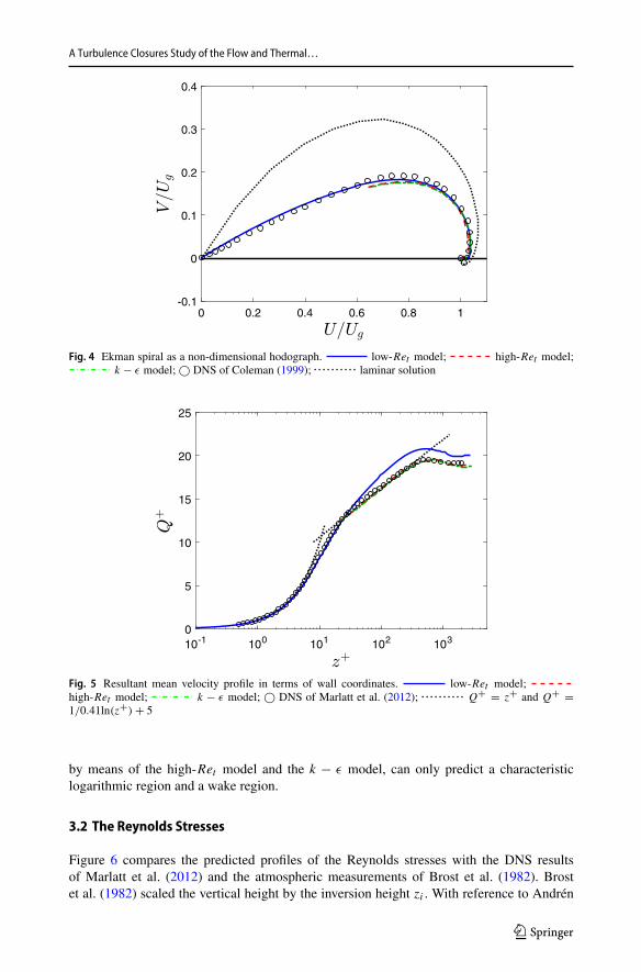
Figure 4 shows the predicted mean velocity profiles in the form of a hodograph. Alsoshown there are the DNS results of Coleman et al. (1990) and, for interest, the laminarsolutions (Eqs. 37, 38). The low-Ret model again shows good agreement with the DNSresults, especially near the wall. The k − ε model prediction is close to the high-Ret modeland both predictions agree well with the DNS; there is only a slight underprediction of Vnear the wall. The high-Ret model and the k − ε model fail to provide a simulation of thewhole Ekman hodograph, because the first node is placed in the logarithmic layer, at z+ ofaround 25, while the low-Ret model is applied directly to the surface.

The model predictions of the resultant mean velocity magnitude Q are plotted in wallcoordinates in Fig. 5 where they are compared with the DNS results of Marlatt et al. (2012).Also shown there are the standard profiles for the viscous sublayer (Q+ = z+) and forthe fully-turbulent flow (Eq. 36). The low-Ret model follows the viscous sublayer profileuntil z+ ≈ 6 and agrees well with the DNS until z+ ≈ 30. For 30 < z+ < 200, thenon-dimensional velocity Q+, obtained by means of the low-Ret model, still describes alogarithmic region but one with somewhat different slope and intercept than Eq. 36 and theDNS. The reason can be found in an underprediction of the friction velocity Qτ (see Table 3).The high-Ret model result, also shown in Fig. 5, indicates that at z+ ≈ 25, the value forQ+ is fixed to the logarithmic law-of-the-wall. The high-Ret model and the k − ε modelreach nearly the same simulation results for Q+. Both models follow fairly closely to boththe law-of-the-wall and to the DNS, since the absolute friction velocity is obtained by meansof the logarithmic law-of-the-wall and the mean profiles of U and V are correctly predicted(see Fig. 4). In summary, although Q+, obtained with the low-Ret model, partially deviatesfrom the DNS and empirical predictions, it still predicts the characteristic velocity profilecomposed of a viscous sublayer, a logarithmic layer and a wake region, while Q+, obtained

123

A Turbulence Closures Study of the Flow and Thermal…

0 0.2 0.4 0.6 0.8 1-0.1

0

0.1

0.2

0.3

0.4

Fig. 4 Ekman spiral as a non-dimensional hodograph. low-Ret model; high-Ret model;k − ε model; © DNS of Coleman (1999); laminar solution

10-1 100 101 102 1030

5

10

15

20

25

Fig. 5 Resultant mean velocity profile in terms of wall coordinates. low-Ret model;high-Ret model; k − ε model; © DNS of Marlatt et al. (2012); Q+ = z+ and Q+ =1/0.41ln(z+) + 5

by means of the high-Ret model and the k − ε model, can only predict a characteristiclogarithmic region and a wake region.

3.2 The Reynolds Stresses

Figure 6 compares the predicted profiles of the Reynolds stresses with the DNS resultsof Marlatt et al. (2012) and the atmospheric measurements of Brost et al. (1982). Brostet al. (1982) scaled the vertical height by the inversion height zi . With reference to Andrén

123

L. Braun et al.

0 1 2 3 4 5 6 70

0.2

0.4

0.6

0.8

1

0 0.5 1 1.5 2 2.50

0.2

0.4

0.6

0.8

1

0 0.5 1 1.5 2 2.50

0.2

0.4

0.6

0.8

1

-1.5 -1 -0.5 0 0.5

-0.2 0 0.2 0.4 0.6 0.8 1

-0.4 -0.2 0 0.2

Fig. 6 Normal (left) and shear (right) Reynolds stresses. low-Ret model; high-Ret model;k − ε model; © DNS of Marlatt et al. (2012); � DNS of Coleman (1999); atmospheric data of

Brost et al. (1982)

(1991), who relied on observations, the atmospheric data are rescaled by using the assumptionzi = 0.4Qτ / f .

In general, the normal stresses exhibit a broadly similar behaviour. Until the streamwisevelocity component U reaches the geostrophic wind speed, u2 is dominant, whereas v2

becomes dominant in the supergeostrophic region. As also mentioned inMarlatt et al. (2012),the surface impedes the vertical fluctuations,which is evident in the lowvalue ofw2 comparedto the other normal stresses.

123

A Turbulence Closures Study of the Flow and Thermal…

The normal stresses u2 and w2 obtained by Marlatt et al. (2012) reach a maximum inthe viscous sublayer, whereas the normal stresses obtained with the low-Ret model reach amaximum in the logarithmic region at about z+ ≈ 35. The normal stresses obtained withthe high-Ret model and the k − ε model both reach their maximum at the first node, fixedat z+ ≈ 25. The k − ε model fails to closely match DNS results partly because, beingbased on the Boussinesq assumption and the flow being fully developed, it predicts all threecomponents of normal stress to be equal. The low- and high-Ret model achieve similar resultsfor z+ > 25 and both models underpredict the maximum values of u2 and w2. However, thepredicted maximum of v2 is very close to the DNS of Marlatt et al. (2012). Both Reynolds-stress transport models therefore provide generally satisfactory results compared to DNSdata. As the normal stress results are in the range of the atmospheric data of Brost et al.(1982), the current simulation seems to reproduce real atmospheric conditions.

The turbulent shear stresses are compared with the DNS results of Marlatt et al. (2012)and Coleman (1999) in Fig. 6. The maximum value of −uw near the wall is reproduced bestby means of the high-Ret model and the k − ε model. However, the profile obtained with thek − ε model deviates from the DNS results farther away from the wall. The low-Ret modelunderpredicts the maximum of −uv provided by Marlatt et al. (2012) and Coleman (1999).However, the location of the maximum at z+ ≈ 16 corresponds with Marlatt et al. (2012)(maximum at z+ ≈ 12). In contrast, the k − ε model predicts this component of shear stressto be zero everywhere as a consequence of ∂U/∂ y and ∂V /∂x being zero in this horizontallyhomogeneous, fully-developed flow. The shear stress−vw profile obtained with the low-Retmodel provides a very good approximation of the DNS results of Coleman (1999), besides anunderprediction of the near-wall minimum value. The change of sign of −uv correlates with−vw at z+ ≈ 50 and appears where the lateral velocity component V reaches its maximum.This location is close to the prediction of Marlatt et al. (2012) at z+ ≈ 58. The low-Retmodel and the k − ε model results are similar for −vw, while the high-Ret model deviatesfrom both models for 0.2 < z f /Qτ < 0.5. The low-Ret model predicts the location of theReynolds stress peaks correctly and the obtained profiles agree with the DNS. However, thenear-wall peak values of u2, w2, and −uv are underpredicted. The stress profiles, obtainedwith the high-Ret model are close to the profiles obtained with the low-Ret model. Thus ifdetailed predictions of the Reynolds-stress profiles in the viscous sublayer are not of interest,there would be little advantage in using the low-Ret model in preference to the high-Retmodel.

An interesting result to emerge from the present simulation concerns the lateral velocitycomponent V , specifically its vertical gradient ∂V /∂z and the turbulent shear-stress compo-nent −vw that enters into its equation (Eq. 3). In a two-dimensional boundary layer, thesetwo quantities are of the same sign as suggested by the Boussinesq assumption. In the Ekmanlayer, the vertical profile of V resembles that of a wall jet (Fig. 3). Due to turbulent trans-port, the location where −vw = 0 in the wall jet does not coincide with the location where∂V /∂z = 0 but lies in-board of it, closer to the surface (Irwin 1973). This is also obtainedin our simulations with the Reynolds-stress models where the shear stress becomes zero atz f /Qτ = 0.040while the velocity gradient becomes zero at a value of 0.046. The k−ε modelobtains the two locations as coincident but this does not appear to have caused significanterrors in its results.

A characteristic of three-dimensional flows such as the Ekman layer is that the angles thatthe resultants of the velocity, the velocity gradients and the shear stress make with the x-axisare not equal and, further, they vary in the vertical direction. These angles are defined as

123

L. Braun et al.

-200 -150 -100 -50 0 500

0.2

0.4

0.6

0.8

1

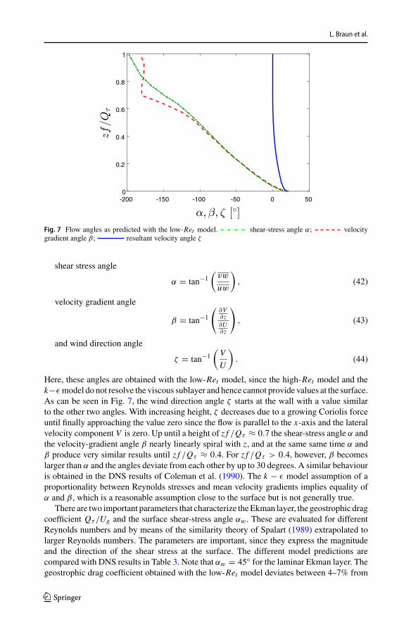
Fig. 7 Flow angles as predicted with the low-Ret model. shear-stress angle α; velocitygradient angle β; resultant velocity angle ζ

shear stress angle

α = tan−1(

vw

uw

), (42)

velocity gradient angle

β = tan−1

(∂V∂z∂U∂z

), (43)

and wind direction angle

ζ = tan−1(V

U

). (44)

Here, these angles are obtained with the low-Ret model, since the high-Ret model and thek−ε model do not resolve the viscous sublayer and hence cannot provide values at the surface.As can be seen in Fig. 7, the wind direction angle ζ starts at the wall with a value similarto the other two angles. With increasing height, ζ decreases due to a growing Coriolis forceuntil finally approaching the value zero since the flow is parallel to the x-axis and the lateralvelocity component V is zero. Up until a height of z f /Qτ ≈ 0.7 the shear-stress angle α andthe velocity-gradient angle β nearly linearly spiral with z, and at the same same time α andβ produce very similar results until z f /Qτ ≈ 0.4. For z f /Qτ > 0.4, however, β becomeslarger than α and the angles deviate from each other by up to 30 degrees. A similar behaviouris obtained in the DNS results of Coleman et al. (1990). The k − ε model assumption of aproportionality between Reynolds stresses and mean velocity gradients implies equality ofα and β, which is a reasonable assumption close to the surface but is not generally true.

There are two important parameters that characterize theEkman layer, the geostrophic dragcoefficient Qτ /Ug and the surface shear-stress angle αw . These are evaluated for differentReynolds numbers and by means of the similarity theory of Spalart (1989) extrapolated tolarger Reynolds numbers. The parameters are important, since they express the magnitudeand the direction of the shear stress at the surface. The different model predictions arecompared with DNS results in Table 3. Note that αw = 45◦ for the laminar Ekman layer. Thegeostrophic drag coefficient obtained with the low-Ret model deviates between 4–7% from

123

A Turbulence Closures Study of the Flow and Thermal…

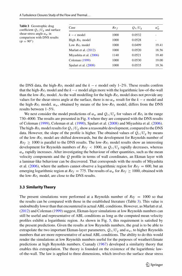
Table 3 Geostrophic dragcoefficient Qτ /Ug and surfaceshear-stress angle αw incomparison with DNS results(φ = 90◦)

Case Re f Qτ /Ug α◦w

k − ε model 1000 0.0532 -

High Ret model 1000 0.0528 -

Low Ret model 1000 0.0499 19.41

Marlatt et al. (2012) 1000 0.0520 18.56

Miyashita et al. (2006) 1140 0.0521 19.40

Coleman (1999) 1000 0.0530 19.00

Spalart et al. (2008) 1000 0.0535 19.36

the DNS data, the high-Ret model and the k − ε model only 1–2%. These results confirmthat the high-Ret model and the k−ε model align more with the logarithmic law-of-the-wallthan the low-Ret model. As the wall modelling for the high-Ret model does not provide anyvalues for the shear-stress angle at the surface, there is no αw result for the k − ε model andthe high-Ret model. αw , obtained by means of the low-Ret model, differs from the DNSresults between 1–5%.

We next consider the model predictions of αw and Qτ /Ug for values of Ret in the range730–4000. The results are presented in Fig. 8 where they are compared with the DNS resultsof Coleman (1999), Coleman et al. (1990), Spalart et al. (2008) and Miyashita et al. (2006).The high-Ret model results for Qτ /Ug showa reasonable development, compared to theDNSdata. However, the slope of the profile is higher. The obtained values of Qτ /Ug by meansof the low-Ret model are shifted downwards, but the development for Reynolds number ofRef ≥ 1000 is parallel to the DNS results. The low-Ret model results show an interestingdevelopment for Reynolds numbers of Ref < 1000, as Qτ /Ug rapidly decreases, whereasαw rapidly increases. After investigating the behaviour of other quantities, such as the meanvelocity components and the Q profile in terms of wall coordinates, an Ekman layer witha laminar-like behaviour can be discovered. That corresponds with the results of Miyashitaet al. (2006), where the authors cannot observe a logarithmic region for Ref = 600, but anemerging logarithmic region at Ref = 775. The results of αw for Ref ≥ 1000, obtained withthe low-Ret model, are close to the DNS results.

3.3 Similarity Theory

The present simulations were performed at a Reynolds number of Ref = 1000 so thatthe results can be compared with those in the established literature (Table 3). This value isundoubtedly lower than that encountered in actual ABL conditions. However, asMarlatt et al.(2012) and Coleman (1999) suggest, Ekman-layer simulations at low Reynolds numbers canstill be useful and representative of ABL conditions as long as the computed mean velocityprofiles exhibit a logarithmic region. As shown in Fig. 5, this requirement is satisfied bythe present predictions. Given the results at low Reynolds numbers, the goal is to be able toextrapolate the two important Ekman-layer parameters, Qτ /Ug and αw , to higher Reynoldsnumbers that are more representative of actual ABL conditions. The ability to do this wouldrender the simulations at low Reynolds numbers useful for the purposes of weather/climatepredictions at high Reynolds numbers. Csanady (1967) developed a similarity theory thatenables this extrapolation. The theory is founded on the existence of the logarithmic law-of-the-wall. The law is applied to three dimensions, which involves the surface shear stress

123

L. Braun et al.

0.035

0.04

0.045

0.05

0.055

0.06

0.065

0.07

0 1 2 3 4 510

15

20

25

30

35

40

Fig. 8 Variation of the geostrophic drag coefficient Qτ /Ug (top) and surface shear-stress angle αw withReynolds number. © low-Ret model; high-Ret model; ×k − ε model; + DNS of Miyashita et al. (2006);� DNS of Coleman et al. (1990); ♦ DNS of Coleman (1999); � DNS of Spalart et al. (2008)

αw . Spalart (1989) found that Csanady (1967) theory did not agree with simulation at lowReynolds numbers (Re f = 500−767) and proposed amodification that involved the additionof a higher-order term and an additional equation

A = Ug

Qτ

sinθw, (45)

B = Ug

Qτ

cosθw + 2

κlnUg

Qτ

− 2

κRe f + 1

κln2, (46)

θw = αw + 2C5

Re2f

(Ug

Qτ

)2

. (47)

Equations 45 and 46 represent Csanady (1967) theory but with the actual surface shearangle αw replaced by a shifted angle θw as defined by Eq. 47. A number of coefficientsare involved, of which the von Kármán constant κ is assigned its usual value of 0.41. Theremaining three constants (A, B, and C5) are obtained by substituting the DNS results into

123

A Turbulence Closures Study of the Flow and Thermal…

Table 4 Determination of thesimilarity theory constants A andB (κ = 0.41 and C5 = −52)

Re f Qτ /Ug αw◦ θw

◦ A B

2000 0.04469 15.46 15.45 5.960 1.342

2500 0.04322 14.63 14.62 5.841 1.237

3000 0.04187 14.29 14.28 5.893 1.259

4000 0.03956 13.60 13.60 5.942 1.557

Average 5.909 1.349

Eqs. 45–47. Coleman et al. (1990), using the DNS results for Re f = 400 and Re f = 500and C5 = −52, obtained the extrapolated results shown in Fig. 9. We revisit this approachby using the results from our low-Ret model to evaluate the constants A and B only nowwith the benefit of having data from much higher values of Re f than those used by Colemanet al. (1990). The outcome of this re-evaluation is presented in Table 4. Note that accordingto Coleman (1999), the modification of the surface shear stress angle, θw , is needed whenRe f < 5000, which is the case here. Subsequently, A and B are calculated by Eqs. 45 and 46at each Reynolds number. As can be seen in Table 4, the obtained values are not very differentfrom each other and, when averaged, yield the values of A = 5.91 and B = 1.35.

In Fig. 9, the extrapolated values of the geostrophic drag coefficient Qτ /Ug and the surfaceshear angle αw as obtained using the averaged values of A and B and those of Coleman et al.(1990) are compared. In presenting the results obtained with our model, a continuous lineis used to designate the range of Re f values used to evaluate A and B, and a dashed line toshow the range over which the results have been extrapolated. We subsequently performedcalculations at three significantly higher values of Re f viz. 10, 000, 20, 000, and 40, 000 toexplore the extent to which the model results agreed with similarity theory together with theaveraged values of A and B. As can be seen from Fig. 9, the results are quite close whichsuggests that similarity theory can yield useful results despite the many assumptions invokedin its formulation.

3.4 Mean Temperature Profile

Thepredictedmean temperature profiles are shown inFig. 10 as a functionof non-dimensionalheight. Since, for air, Pr < 1, the thermal boundary layer is slightly thicker than the momen-tum boundary layer and hence the mean temperature profile and the turbulent heat fluxes arepresented for 0 ≤ z f /Qτ ≤ 1.5. The difference between the explicit algebraic model and thedifferential transport model is insignificant. However, the mean temperature profile obtainedwith Fourier’s law departs from the other two models by providing smaller temperature val-ues for z f /Qτ > 0.06. This result is entirely due to assigning the turbulent Prandtl number aconstant value of 0.85. By assigning the higher value of 1 implied by the alternative models,all the predicted temperature profiles become virtually indistinguishable from each other.

Figure 11 shows themean temperature profiles plotted in wall coordinates in order to com-pare the simulation results with a law-of-the-wall for temperature, proposed by Duponcheelet al. (2014)

�+ = � − �w

�τ

= Prtκ

ln

(1 + Pr

Prtκ z+

), (48)

where the friction temperature �τ is defined as

123

L. Braun et al.

0

0.01

0.02

0.03

0.04

0.05

0 10 20 30 400

5

10

15

20

Fig. 9 Similarity theory and low-Ret model results for the variation of geostrophic drag coefficient (top) andsurface shear stress angle with Re f . Present values (Table 4): fitted curve; extrapolatedcurve. Coleman et al. (1990) values of A and B: . © low-Ret model predictions

�τ =λ

(∂�∂z

)z=0

ρcpQτ

. (49)

Here λ is the thermal conductivity and cp is the specific heat at constant pressure. The lawwas developed for low Prandtl numbers with the goal of offering an accurate wall functionfor high-Ret models. The authors derived Eq. 48 from the heat-flux conservation near thewall, without neglecting the turbulent thermal diffusivity Kh . The formulation does notneed a blending function (such as that proposed by Kader 1981), which links the linear lawclose to the wall with the logarithmic further away from the wall. Equation 48 approaches�+ = Pr z+ for small z+, which fulfills the requirement of a laminar law in the near-wallregion. The predicted mean temperature profile generally agrees with the law-of-the-wall forz+ < 200, but the slope of both the algebraic and the differential heat-flux model is higherthan the slope obtained with Eq. 48. Nevertheless, the proposed function of Duponcheel et al.(2014) could be a useful wall function for a high-Ret heat transfer simulation of the Ekmanlayer.

123

A Turbulence Closures Study of the Flow and Thermal…

0 0.2 0.4 0.6 0.8 10

0.5

1

1.5

Fig. 10 Predicted vertical profiles of mean potential temperature. differential transport model;non-linear model; Fourier’s law (Prt = 0.85)

10-1 100 101 102 1030

2

4

6

8

10

12

14

16

18

Fig. 11 Mean temperature profile in wall coordinates. differential transport model; non-linear model; Fourier’s law; law of the wall for temperature of Duponcheel et al. (2014)(Eq. 48 with Pr = 0.71, Prt = 0.85, κ = 0.41)

3.5 Turbulent Heat Fluxes

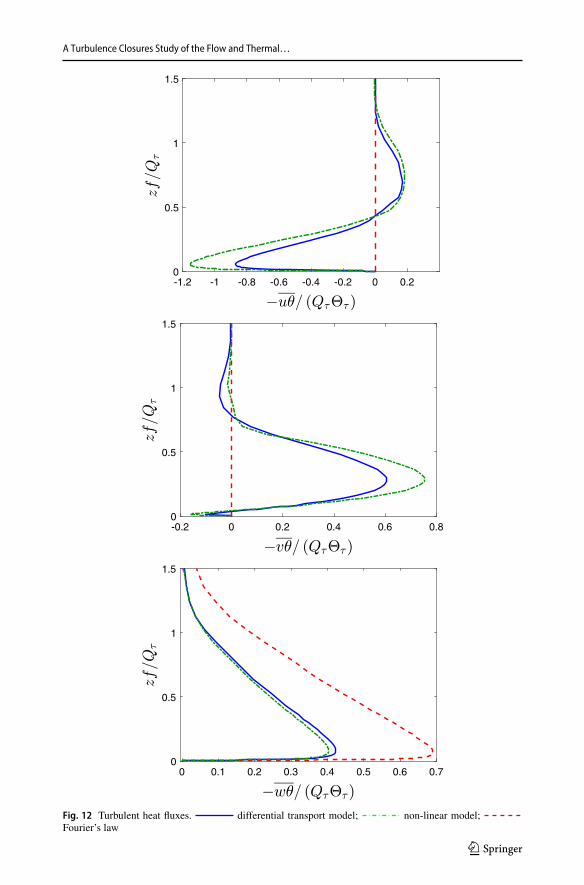
The predicted vertical profiles of the turbulent heat fluxes obtained with the various modelsare presented in Fig. 12. The fluxes are non-dimensionalized by the friction velocity and thefriction temperature. It is interesting to note that the largest of the heat fluxes occurs in thestreamwise direction (uθ ) even though the only temperature gradient that is finite is in thevertical direction. The Fourier law cannot predict the conductive heat transfer, as the lawdoes not consider velocity gradients and Reynolds stresses. At the same time, the maximumvalue of the vertical heat flux departs from the differential and algebraic models by ≈ 60%.The differential model and the algebraic model predict different maximum values of −uθ

123

L. Braun et al.

and −vθ . However, the location of these maxima is the same. The difference between bothmodels in the prediction of −wθ is insignificant.

3.6 EddyViscosity, Diffusivity and the Turbulent Prandtl Number

Predicted andmeasured vertical profiles of the turbulent viscosity Km are presented in Fig. 13.Plotted there is the single (isotropic) profile obtained with the k − ε model (Eq. 9), and twoprofiles that are implied in the RSM but that do not enter into the computations viz.

Km13 = −uw

∂U/∂z, (50)

Km23 = −vw

∂V /∂z. (51)

The discontinuous behaviour obtained for Km23 is characteristic of that obtained in a wall jetand arises because ∂V /∂z passes through zero. With increase in vertical distance, the eddyviscosities Km13 and Km23 move closer together suggesting that departures from isotropyare quite small. The isotropic eddy viscosity is seen to closely follow the Km13 distributionacross a significant depth of the Ekman layer.

The components of eddy viscosity are sometimes presented in the literature not as indi-vidual components but in an averaged form. Marlatt et al. (2012) define the average viscosityas

Km = [uw2 + vw2]0.5

[(∂U

∂z

)2

+(

∂V

∂z

)2]−0.5

. (52)

The profiles of the averaged eddy viscosity as deduced from the DNS results of Marlatt et al.(2012) and the experimental data of Caldwell et al. (1972) are presented in Fig. 13 (notethat the Caldwell et al. (1972) results pertain to the somewhat higher Reynolds number ofRe f = 1159). Because theRSMpredicted profiles of Km13 and Km23 are essentially identical,their individual profiles turn out to be essentially identical to the profile of their average asevaluated from Eq. 52. In the inner layer, remarkably close correspondence between theRSM and DNS results is observed though the RSM results do not capture the non-monotonicbehaviour seen in the DNS results.

Profiles of the eddy diffusivity Kh are presented in Fig. 14. For the non-linear and differ-ential models, this parameter is obtained from

Kh = −wθ

∂�/∂z, (53)

and is presented in Fig. 14 as a function of non-dimensional height. The differential and non-linear algebraic models yield closely-matched results that indicates that the diffusive andconvective processes are relatively small. In contrast, Fourier’s law, with a constant Prandtlnumber of 0.85, yields substantially different results. There are no DNS or experimentaldata to confirm these results. By using Eqs. 52 and 53, the turbulent Prandtl number cannow be calculated using the models predictions. The results are shown in Fig. 15 where itcan be seen that the models indicate that the turbulent Prandtl number depends on height,especially in the near-wall region (z f /Qτ < 0.05), with average values that can exceed1.1. This finding is in good accord with results from several semi-empirical models for thenear-wall behaviour of turbulent Prandtl number in laboratory flows (Kays et al. 2005). Li(2019) reviewed alternative models for the turbulent Prandtl number in the neutral ABL and

123

A Turbulence Closures Study of the Flow and Thermal…

-1.2 -1 -0.8 -0.6 -0.4 -0.2 0 0.20

0.5

1

1.5

-0.2 0 0.2 0.4 0.6 0.80

0.5

1

1.5

0 0.1 0.2 0.3 0.4 0.5 0.6 0.70

0.5

1

1.5

Fig. 12 Turbulent heat fluxes. differential transport model; non-linear model;Fourier’s law

123

L. Braun et al.

0 0.01 0.02 0.03 0.04 0.05 0.06 0.070

0.05

0.1

0.15

0.2

0.25

0.3

Fig. 13 Vertical profiles of eddy viscosity. high-Ret model Km13 ; high-Ret model Km23 ;k − ε model; © DNS results of Marlatt et al. (2012); experimental data of Caldwell et al. (1972)

(Re f = 1159)

0 0.02 0.04 0.06 0.08 0.10

0.05

0.1

0.15

0.2

0.25

0.3

Fig. 14 Vertical profiles of eddy diffusivity. differential transport model; non-linear model;Fourier’s law

found that different theories yield values that are higher than 0.85. Repeating the Fourier lawcalculations with Prt = 1.0 produced temperature profiles that were virtually identical tothe those obtained with the differential and the non-linear models.

123

A Turbulence Closures Study of the Flow and Thermal…

0.7 0.8 0.9 1 1.1 1.20

0.05

0.1

0.15

0.2

0.25

0.3

Fig. 15 Turbulent Prandtl number as a function of height above surface. differential transport model;non-linear model; Prt = 0.85

4 Conclusions

The turbulent Ekman layer provides a simple model for the ABL and hence the interest indeveloping turbulent closures that can accurately predict its flow and thermal fields. Theresults presented above indicate that the k − ε turbulence model, in its standard form, canbe relied upon to capture the main features of this flow such as the vertical distribution ofthe mean velocity components. When presented in wall coordinates, these model resultsaccurately reproduce the logarithmic-law profile obtained from the DNS results of Marlattet al. (2012). The geostrophic drag coefficient was also well predicted with this model.Because attention here was confined to fully-developed flow, the normal stresses obtainedby the Boussinesq assumption are obtained as being equal whereas in reality turbulence ishighly anisotropic due to the damping effects of the surface. On the other hand, the turbulentshear stresses were reasonably well predicted.

Concerning the Reynolds-stress transport models, results obtained with high- and low-Ret variants of the same basic model were quite similar for the vertical profiles of the meanvelocity components and the Reynolds stresses. The use of the logarithmic law-of-the-wallto provide boundary conditions for the high-Ret model does not appear to have adverselyaffected its overall performance, though having to apply these conditions at some distanceaway from the surface meant that only the low Ret model was capable of reproducing theentire Ekman spiral. Examination of the predicted directions of the resultant turbulent shearstresses and the associated gradients ofmean velocity gradients showed these to be coincidentacross the vertical extent of the Ekman layer. Furthermore, analysis of the predicted verticalprofiles of the eddy viscosities Km13 and Km23 showed these to be reasonably equal except fora small region close to the surface where Km23 was discontinuous where the lateral velocitycomponent V was at a maximum and hence ∂V /∂z, which appears in the denominator,was identically zero. This result indicates that the assumption of isotropic eddy viscosity inlower-order models such as the k − ε is quite acceptable in this flow.

123

L. Braun et al.

Even though the focus of the study was on the case of Re f = 1000 and a latitude of 90◦ N,the conditions for which the majority of DNS results are available, the results obtained withthe low-Ret model were used to in conjunction with the similarity theory of Spalart (1989)to obtain predictions at Re f values more representative of those encountered in the ABL.Subsequent predictions with the low-Ret model for values of Re f up to 40, 000 agreed verywell with extrapolated similarity theory results.

For weather predictions, the computational cost of turbulence models is an importantparameter. Since the high Ret model yields as good results as the low Ret alternative butwith less computational cost, there is no justification for using the more complex and com-putationally more demanding model. However, if the simulation of flow very close to thesurface is of interest, then the only available option would be to perform the calculationsdirectly to the wall.

The thermal field predictions obtained with a non-linear algebraic heat-flux model andthe more complex differential transport model showed no significant differences in termsof the vertical profiles of the mean temperature and the heat fluxes. In contrast, Fourier’slaw, even when used in conjunction with the Reynolds-stress model, produced a temperaturedistribution that is vastly different from the other models. These model results can be broughtin line with the others simply by assigning to the turbulent Prandtl number a value of 1 insteadof its more usual value of 0.85.

Acknowledgements Lukas Braun gratefully acknowledges the financial support provided by the Studiens-tiftung des deutschen Volkes that facilitated this research at UC Davis.

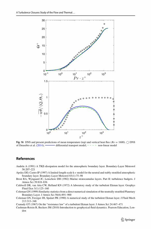
Appendix: Comparisons with the DNS of Deusebio et al. (2014)

A reviewer drew our attention to the DNS results of Deusebio et al. (2014) for the meantemperature and vertical heat flux in a neutrally-stratified Ekman layer. These results arepresented in Fig. 16 where they are compared with the present predictions. In the viscoussub-layer (z+ < 8), the correspondence between the DNS results for mean temperature andthe predictions of the differential and the non-linear flux models is quite close. However,differences appear further away from the surface. There, the pronounced change in the slopeof the temperature profile exhibited by the DNS is not reproduced in the models’ predictions.Concerning the vertical turbulent heat flux, significant differences between the present resultsand the DNS are apparent. We are at a loss to explain the observed differences in the profilesshape, especially in the outer region of the boundary layer where the DNS results show anextensive region of constant heat flux. We are however encouraged to see that the two modelsyield almost identical results even though they differ in so many ways (e.g. algebraic vs.differential), and share no assumptions in their formulation.

123

A Turbulence Closures Study of the Flow and Thermal…

10-1 100 101 102 1030

5

10

15

20

25

30

100 101 102 1030

0.5

1

1.5

Fig. 16 DNS and present predictions of mean temperature (top) and vertical heat flux (Re = 1600). © DNSof Deusebio et al. (2014); differential transport model; non-linear model

References

Andrén A (1991) A TKE-dissipation model for the atmospheric boundary layer. Boundary-Layer Meteorol56:207–221

Apsley DD, Castro IP (1997) A limited-length-scale k-ε model for the neutral and stably stratified atmosphericboundary layer. Boundary-Layer Meteorol 83(1):75–98

Brost RA, Wyngaard JC, Lenschow DH (1982) Marine stratocumulus layers. Part II: turbulence budgets. JAtmos Sci 39:818–836

Caldwell DR, van Atta CW, Helland KN (1972) A laboratory study of the turbulent Ekman layer. GeophysFluid Dyn 3(1):125–160

ColemanGN (1999) Similarity statistics from a direct numerical simulation of the neutrally stratified PlanetaryBoundary Layer. J Atmos Sci 56(6):891–900

Coleman GN, Ferziger JH, Spalart PR (1990) A numerical study of the turbulent Ekman layer. J Fluid Mech213:313–348

Csanady GT (1967) On the “resistance law” of a turbulent Ekman layer. J Atmos Sci 24:467–471Cushman-Roisin B, Beckers JM (2010) Introduction to geophysical fluid dynamics. Pearson Education, Lon-

don

123

L. Braun et al.

Daly BJ, Harlow FH (1970) Transport equations in turbulence. Phys Fluids 13(11):2634–2649Detering HW, Etling D (1985) Application of the E-ε turbulence model to the atmospheric boundary layer.

Boundary-Layer Meteorol 33(2):113–133Deusebio E, Brethouwer G, Schlatter P, Lindborg E (2014) A numerical study of the unstratified and stratified

Ekman layer. J Fluid Mech 755:672–704Duponcheel M, Bricteux L, Manconi M, Winckelmans G, Bartosiewicz Y (2014) Assessment of RANS and

improved near-wall modeling for forced convection at low Prandtl numbers based on LES up to Re=2000.Inl J Heat Mass Transf 75:470–482

Gibson MM, Launder BE (1978) Ground effects on pressure fluctuations in the atmospheric boundary layer.J Fluid Mech 86(3):491–511

Irwin HPAH (1973) Measurements in a self-preserving plane wall jet in a positive pressure gradient. J FluidMech 61:33–63

Johnstone JP, FlackKA (1996)Review—advances in three-dimensional turbulent boundary layerswith empha-sis on the wall-layer regions. J Fluids Eng 118:219–232

Kader BA (1981) Temperature and concentration profiles in fully turbulent boundary layers. Int J Heat MassTransf 24(9):1541–1544

KannepalliC, PiomelliU (2000)Large-eddy simulationof a three-dimensional shear-driven turbulent boundarylayer. J Fluid Mech 423:175–203

KaysW, Crawford M,Weigand B (2005) Convective heat and mass transfer, 4th edn. McGraw Hill, New YorkKays WM (1994) Turbulent Prandtl number—where are we? J Heat Transf 116(2):284–295Kebede W, Launder BE, Younis BA (1985) Large-amplitude periodic pipe flow: a second-moment closure

study. In: 5th symposium on turbulent shear flow, pp 1623–1629Launder BE (1976) Heat and mass transfer, Chap. 6. In: Bradshaw P (ed) Turbulence, vol 12. Topics in applied

physics. Springer, Berlin, pp 231–287Launder BE, Spalding DB (1972) Lectures in Mathematical models of turbulence. Academic Press, LondonLi D (2019) Turbulent Prandtl number in the atmospheric boundary layer—where are we now? Atmos Res

216:86–105Malin MR, Younis BA (1990) Calculation of turbulent buoyant plumes with a Reynolds stress and heat flux

transport closure. Int J Heat Mass Transf 33(10):2247–2264Marlatt S, Waggy S, Biringen S (2012) Direct numerical simulation of the turbulent Ekman layer: evaluation

of closure models. J Atmos Sci 69:1106–1117Mauritsen T, Svensson G, Zilitinkevich SS, Esau I, Enger L, Grisogono B (2007) A total turbulent energy

closure model for neutrally and stably stratified atmospheric boundary layers. J Atmos Sci 64:4113–4126Miyashita K, Iwamoto K, Kawamura H (2006) Direct numerical simulation of the neutrally stratified turbulent

Ekman boundary layer. J Earth Simulator 6:3–15Momen M, Bou-Zeid E (2017) Mean and turbulence dynamics in unsteady Ekman boundary layers. J Fluid

Mech 816:209–242Müller H, Younis BA, Weigand B (2015) Development of a compact explicit algebraic model for the turbulent

heat fluxes and its application in heated rotating flows. Int J Heat Mass Transf 86:880–889Schlichting H, Gersten K (2006) Grenzschicht-Theorie, 10th edn. Springer, BerlinSogachevA,KellyM,LeclercMY(2012)Consistent two-equation closuremodelling for atmospheric research:

buoyancy and vegetation implementations. Boundary-Layer Meteorol 145:307–327Sous D, Sommeria J (2012) A Tsai’s model based S-PIV method for velocity measurements in a turbulent

Ekman layer. Flow Meas Instrum 26:102–110Spalart PR (1989) Theoretical and numerical study of a three-dimensional turbulent boundary layer. J Fluid

Mech 205:319–340Spalart PR, Coleman GN, Johnstone R (2008) Direct numerical simulation of the Ekman layer: a step in

Reynolds number, and cautious support for a log law with a shifted origin. Phys Fluids 20(10):101507Wilcox DC (1993) Turbulence modeling for CFD. DCW Industries Inc, La CãnadaWirthA (2010)On theEkman spiralwith an anisotropic eddy viscosity. Boundary-LayerMeteorol 137(2):327–

331Younis BA (1987) EXPRESS: a computer programme fortwo-dimensionalturbulent boundary layer flows.

Department of CivilEngineering, City University, LondonYounis BA, Speziale CG, Berger SA (1998) Accounting for the effects of system rotation on the pressure-strain

correlation. AIAA J 36(9):1746–1748

123

A Turbulence Closures Study of the Flow and Thermal…

Younis BA, Speziale CG, Clark TT (2005) A rational model for the turbulent scalar fluxes. Proc R Soc AMathPhys Eng Sci 461(2054):575–594

Younis BA, Weigand B, Laqua A (2012) Prediction of turbulent heat transfer in rotating and nonrotatingchannels with wall suction and blowing. J Heat Transf 134(7):071702

Publisher’s Note Springer Nature remains neutral with regard to jurisdictional claims in published maps andinstitutional affiliations.

123