a transfer-matrix monte carlo study of random penrose tilingsa transfer-matrix monte carlo study of...
TRANSCRIPT
J. Phyr. A: Math. Gen. 24 (1991) 4129-4153. Printed in the U K
A transfer-matrix Monte Carlo study of random Penrose tilings
Laurence J Shaw and Christopher L Henleyt Department of Physics, Cornell University, Ithaca, NY 14853-2501, USA
Received 6 July 1990, in final form 26 April 1991
Abstract. We investigate the entropic properties of a simple two-dimensional random quasicrystal model: a random tiling by the 36'and 72'rhombi. Applying the transfer matrix Monte Carla (TMMC) method to random tilings for the first time, we have calculated the entropy as a function of phasan strain. We confirm earlier results that the slate of zero phasan strain (i.e. ten-fold symmetry) has the largest entropy; the entropy is 0.4810 ( 5 ) per tile. In addition, by fitting the dependence ofthe entropy on the pharon strain wedetermined the three stiffness constants in the phason elasticity, one of which is not measurable by previous approaches. We compare the efficacy of the TMMC method with that of other methods.
1. Introduction
1.1. Theoretical and experimental background
Since the first identification of materials with non-crystallographic long-range order in 1984 [I] , extensive work has been done in the field [2-41. Still the atomic structure and the thermodynamic mechanisms of formation are unresolved. It is not clear whether the mechanisms of formation are the same for all alloys, or whether a number of different models are needed to explain the broad range of solidification rates and varying amounts of disorder of the different families of quasicrystal forming alloys. There are currently three kinds of model: the icosahedral glass model, the perfect quasicrystal model, and the random tiling model.
Until recently, all quasicrystals were produced by thermal quenching and had a high degree of disorder [5]. Whereas the orientational correlation length was typically a micron, positional correlation lengths were on the order of a few hundred angstroms producing finite width diffraction peaks [6].
The icosahedral glass model [7 ,8] is a non-equilibrium model where the system is grown from a seed icosahedron by adding icosahedra of the same orientation vertex to vertex at random locations; the positional correlation length is finite although the orientational correlation length spans the system. The positions of simulated diffraction peaks are in agreement with experiment [9]. With some annealing of a icosahedral glass growth process the peak widths will scale linearly with the phason momentum in agreement with experiment [lo, 111.
t To whom correspondence should be addressed.
0305-447@/91/174129+25$03.50 0 1991 IOP Publishing Ltd 4129
4130 L I Shaw and C L Henley
The perfect quasicrystal model supposes an energetic ground state with quasiperiodic long-range order [ 121. Like an ideal crystal, its diffraction pattern consists solely of delta-function peaks. The existence of perfect quasicrystals as a ground state requires the unlikely microscopic characteristics of highly specific atomic bonding (in analogy to the matching rules of perfect Penrose tilings).
The random tiling model, on the other hand, supposes the system has many atomic arrangements of almost degenerate energy. The quasicrystal state is a thermal equi- librium phase (as in the perfectly quasiperiodic theory) but the role of disorder is emphasized (as in the icosahedral glass model). The phason fluctuations (see section 2) have an elastic theory of the usual gradient-squared kind. It has been shown that this implies that a random-tiling model has delta-function diffraction peaks in three dimensions [2,13], despite the short-range phason fluctuations. There is a Debye- Waller reduction of intensity, which is transferrred to diffuse scattering; these are determined quantitatively by the values of the stiffness constants. In two-dimensional systems, such as the random Penrose tiling considered in this paper, the diffraction peaks are expected to have a power-law form where the exponent in the power-law is determined by the stiffness constants. The importance of the stiffness constant has motivated our calculation, both for its direct relevance to two-dimensional quasicrystals, and as a test of our transfer-matrix method in view of possible adaptation to the three dimensional case.
In addition, it was hypothesized [13,14] that the random tiling state might be thermodynamically stabilized because of the reduction in free energy from the configur- ational entropy. Models of entropically stabilized long-range order predict that the quasicrystal phase is stable at higher temperatures (less than the melting point) but a related crystal phase of slightly lower energy becomes stable at lower temperatures as the entropy term becomes less significant.
Interest in random tilings has increased since the recent discovery of equilibrium quasicrystals such as i(A1CuFe) [15]. These have resolution limited diffraction peaks indicating long-range order, which is consistent with either the ideal quasicrystal model or the random-tiling model. Furthermore, some experiments have found the equilibrium quasicrystals to undergo a phase transition at lower temperatures to a periodic state [15]. This is contrary to the premises of the ideal quasiperiodic model but in agreement with predictions of the random-tiling model. Further discussion of random tilings and their relevance to experiment may be found in two brief reviews [16,17].
Numerical studies of two- and three-dimensional random tilings confirm the existence of an entropically stabilized quasiperiodic phase [18, 191 i.e. random tilings possess long-ranged quasiperiodic order. Strandburg er a/ (1989) [ 191 have performed Monte Carlo simulations on the two-dimensional binary and unconstrained random tiling models. Unconstrained random tilings (see figure 1) are random tilings of 36" and 72" rhombi, i.e. Penrose rhombi. Binary random tilings are tilings of the Penrose rhombi with colouring restrictions. Binary random tilings may be mapped to disc packings, where the discs have (non-additive) radii 7 and unity. Strandburg et a/ 1191 performed simulations on unconstrained random tilings of up to 3571 rhombi and estimated K =$(K++K_)=0.60+0.02 and K1=0.56+0.03, and on binary random tilings of up to 3571 discs they estimated K =0.627*0.015, where K,, K _ and K : are the independent stiffness constants (see section 2.3). Widom er al [18] calculated the transfer-matrix, and thereby the tiling entropy, exactly for systems with widths Of UP to 13 discs. Using finite-size scaling to extrapolate to the thermodynamic limit, they estimated an entropy density per unit area of 0.2374*0.0003, and K =0.600*0.006,
Transfer-matrix MC of random Penrose riling 4131
in rough agreement with Strandburg et al. Monte Carlo simulations of random tilings of Ammann rhombohedra [20,21] have also confirmed the existence of long-range order in three-dimensions.
1.2. Plan of the paper
Here we investigate the entropic properties of unconstrained (maximally) random Penrose tilings. That is, our ensemble consists of all ways to tile the plane with rhombi of unit edge and acute angles either 36" or 72". The number of possible tilings grows exponentially with the area of the system. Equal weight is given to each distinct configuration; in other words there is n o Hamiltonian but only the tiling constraint (as in other purely entropic models such as hard spheres). It is plausible that the thermodynamic state is ten-fold symmetric, in the sense of having equal distributions of all the different possible orientations of the tiles; however, this does not necessarily imply any degree of long-range order.
To determine the long-wavelength properties, in particular the shape of diffraction peaks, it suffices to know the coarse-grained free energy (which is purely entropy in our case) in terms of the 'phason' degree of freedom. (The latter is defined in section 2.1; it will suffice to say here that ten-fold symmetry corresponds to zero phason strain and any phason strain corresponds to a deviation from this state.) Therefore, the goal of the paper is to calculate the entropy as a function of phason strain. We only consider small phason strains so this reduces to the calculation of the entropy for zero phason strain, and the stiffness constants which are coefficients of the leading terms in the expansion ahout this point.
Since the tiling may be decomposed into layers, a numerical transfer-matrix formula- tion can be used to calculate the thermodynamic properties of the tiling on a strip [14, 18,221. A numerically exact transfer-matrix calculation is formidable except for the narrowest strips, since the dimension of the vector space grows exponentially with the width of the system. The transfer-matrix Monte Carlo (TMMC) method is useful because it does not require storing the transfer-matrix or a complete vector in computer memory. We work with transfer-matrices up to a dimension of approximately 10" x IO" corresponding to a system width of 24 tiles. Although we can use much larger system sizes than with the ordinary, numerically exact transfer matrix technique, the price is the introduction of random statistical errors.
In section 2 we introduce notation and review results of earlier work. In particular, we give the relations between the phason strain and the tile densities, the continuum elastic theory of phason fluctuations, and the transfer-matrix formulation for random Penrose tilings [14]. Section 3 contains new analytic results, extending the earlier work, which are technically necessary in implementing the numerical calculation of the entropy and stiffness constants. In particular, we explain the use of chemical potentials to control the phason strain; show a useful identity of the needed value of the chemical potential with the true entropy per unit area; and derive the dependence of the entropy on the transverse phason strain (the variable we control). Nearly identical results are equally valid for the other two-dimensional tilings with ten-fold symmetry. In section 4 we present results and conclusions. We present a numerically precise determination of the entropy per tile (in the ten-fold symmetric state where it is maximized). Using chemical potentials to deviate from this state, and fitting the variation of the entropy to the known form of the quadratic 'phason' elasticity, we extract estimates for the three independent phason stiffness coefficients K,, K - and K,. (Our approach to the
4132
data analysis is different from that of Widom et a1 [18] who did not separate K , and K.) We also discuss the efficacy of the TMMC method as compared with standard Monte Carlo simulation, or the finite-size scaling of exact transfer-matrix computations for small systems. Appendix A provides the basic theory of the transfer-matrix Monte Carlo method and presents details of the implementation which may be applied to any TMMC calculation. Appendix B presents the particulars of our TMMC implementa- tion for the random Penrose tiling, and discusses our attempts to improve the conver- gence of the method with importance sampling. Appendix C summarizes useful information about the random tiling of 60" rhombi.
L J Shaw and C L Henley
2. Basic theory of random Penrose tilingsi
2.1. Physical and phason space
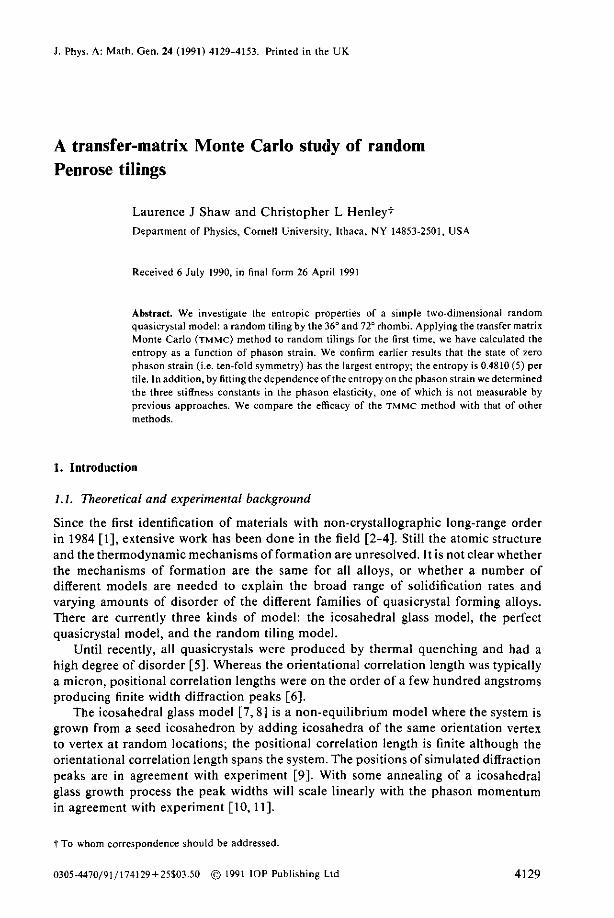
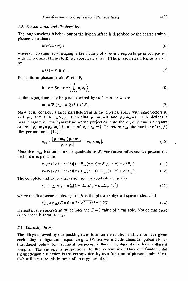
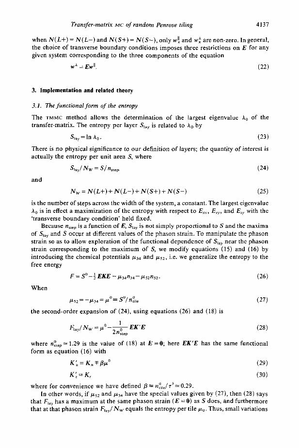
A random Penrose tiling (i.e. a tiling of 36" and 72" rhombi, see figure 1) may be viewed as the projection of a connected two-dimensional hypersurface made of 2-faces of a five-dimensional simple cubic lattice. Each vertex of the tiling is specified by a vector
where n, are integers and
e! = (-sin(Zra/5), cos(2na/5))
as shown in figure 1. Types of tiles are specified by their edge directions. For instance, tiles with edge directions er and e! are called (1,3) (or (3, 1)) tiles. The (a, n + 1) and (a, a +2) tiles are termed thin and fat tiles respectively. The (1,3) and (1,4) tiles will be called thin vertical tiles, and (3,4) and (2,5) tiles will be called fat vertical and thin horizontal tiles respectively.
The e! vectors are projections onto the two-dimensional 'physical space' of the basis vectors of a five-dimensional cubic lattice. The corresponding 'phason' coordinate of the vertex (1) is
wherel
e'= (-sin(4ra/5), cos(4ra/5) , l/A)
and the five-dimensional position is 5
r ' + d = 1 n , ( e : + e l ) " - I
t Corrections to a number of errors in [ I41 are listed here. The ( d l D ) of ( 2 . 6 ) should be replaced with a (dID)' , the 0.9960 in (4.6) should be replaced with 1.2892, the 0.95 in (4.7) should be replaced with 0.8123 and (4.8) should read ( L l N,) = 5/2r2=0.9549. A numerically incorrect entropy value (corrected in our (68) ) is quoted at the end of section 3.2. $The more common definition replaces 4na/5-6ro/S in (4): this merely changes the sign of the X I
components of all pharan vectors.
Transfer-mafrix MC of random Penrose tiling 4133
2.2. Phason strain and file densifies
The long wavelength behaviour of the hypersurface is described by the coarse grained phason coordinate
h(rll) =(r'),ii ( 6 )
where (. . .),IN signifies averaging in the vicinity of r" over a region large in comparison with the tile size. (Henceforth we abbreviate r i l as 1.) The phason strain tensor is given by
E ( r ) = V . h ( r ) .
For uniform phason strain E ( r ) = E,
h + r = E r + r = ( Y = l nee..)
so the hyperplane may be parameterized
(7)
:re
(9)
Now let us consider a large parallelogram in the physical space with edge vectors pm and pa, and area IpexpPl , such that p;m,=O and p,.m,=O. This defines a parallelogram on the hyperplane whose projection onto the e,, e, plane is a square of area (pm.mP) (pp .m, ) in units of le,, x e P l = s . Therefore nap. the number of ( a , P ) tiles per unit area, [14] is
Note that nap has terms up to quadratic in E. For future reference we present the first-order expansions
n34= ( 2 f i / 2 5 ) [ 1 -E,,(T+ I ) + EYy( l -T) - f iE , ]
n 5 , = ( 2 f i / 2 5 ) [ 7 + E,(T- 1) - EJI + ~)+v'?E,,.l.
n,ilc = = n a d - - E,,E,,)/T 1
( 1 1 )
(12)
The complete and exact expression for the total tile density is
(13) 3
=,
where the first/second subscript of E is the phason/physical space index, and
n:,,= n,!,,(E = 0 ) = 2 i 2 f i / 5 = 1.231. (14)
Hereafter, the superscript '0' denotes the E = O value of a variable. Notice that there is no linear E term in n,j,c.
2.3. Elasficify theory
The tilings allowed by our packing rules form an ensemble, in which we have given each tiling configuration equal weight. (When we include chemical potentials, as introduced below for technical purposes, different configurations have different weights.) The entropy is proportional to the system size. Thus our fundamental thermodynamic function is the entropy density as a function of phason strain S ( E ) . (We will measure this in w i t s of entropy per tile.)
4134 L J Shaw and C L Henley
The fundamental conjecture of the random tiling model of quasiperiodic order is that the entropy of the tiling is a quadratic maximum at E =0 , i.e.
where K, the stiffness constant tensor, is positive definite [lo, 141. Group theoretic arguments [23] have been used to identify the number of independent components of K. The functional form of the entropy must be invariant under any rotation of the tiling by a multiple of 72'together with the corresponding rotation about z' in phason space (which is twice the angle, see (4)). This analysis yields three independent stiffness constants which couple components of the phason strain to give:
S = S"-fK+[(E,, + E?,,)*+ (Exy - E,.,)']
-fK_[(E, - E,,.)'+ (E,. + - Kz[E:,+ €$I = so - (K , + K _ ) [ E:, + E:,, + E:, + €3
- 2 ( K + - K-) [ E&", .~ - ExJEYx1- K,[EZ,+ EX]. (16) This work provides the first estimates of both ( K + + K _ ) and ( K + - K _ ) for
decagonal quasiperiodic tilings. The ( K + - K-) contribution to the entropy of a region reduces to an integral over the boundary since
E,,E,-E,,E,=Vx[h,Vh,I (17)
is an exact differential [24]. If one is only interested in the fluctuations about the average phason strain, or if the average phason strain is zero, the (K+ - K - ) term may be neglected. (This is equivalent to converting to Fourier components, i.e. E,, -f q,h,, Ex." -f q,h,, etc.) Thus, Monte Carlo simulations which determine the (entropic) elastic constants by measuring fluctuations around a state can only measure the combination (K++ K)?. This is true whether there is a fixed net phason strain due to the boundary conditions, or whether the system is allowed to find the maximum-entropy state with zero phason strain. Our estimate of the value of (K , - K - ) is of physical importance since, if the global phason strain is not constrained at zero, the sign of (K, - K-) determines the stability of the zero phason strain random tiling as compared to states with non-zero uniform strain, e.g. large rational approximant crystals with random tiling disorder [16].
2.4. E'ling rules and the transfer-matrix
The nearly horizontal dotted lines across figure 1 separate 'layers' of the tiling. The tiling has periodic boundary conditions horizontally. Dotted line segments of length 1, I , 7-' and r-' along e! , -e?, e! , and -e! are termed L+, L-, St and S' steps respectively. For instance, the sequence of steps across the leading (top) layer of figure 1 is {LtL'L~L-S-StL~S-LtS+). Layer lines cut through all thin and fat vertical tiles. A simple counting argument shows that the number of steps per unit area, n,,,,= n ( Lt) + n( L-)+ n(S+) + n ( S - ) , obeys [ 141
(18) flneP = ntilC + n34 - ns2.
t But a Monte Carlo simulation with free boundary conditions, could in principle determine ( K + - K.1, if one measures the global phason strain: this fluctuates according to a statistical weight which is exponential in the system area times the full phason elastic term.
Transfer-matrix M C of random Penrose tiling 4135
Figure 1. A random Penrose tiling configuration. Layer lines are shown broken. (After figure 4 of [141.)
The transition rules assign a weight to each permissible permutation of steps between two layers. These weights form the entries of the transfer-matrix. The tiling of a new layer is determined by the state of the previous layer and the operations performed in the permutation of steps between layerst. The transition rules for generating successive layers may be divided into three stages as follows (see appendix B for TMMC
implementation details): (i) The LL rule is composed of any number of L+L-+ L-Lt exchanges between
nearest-neighbour steps. Thus, the LL rule changes the plus/minus ordering within strings of consecutive L steps; L+ steps can move to the right and the L- steps can move to the left, but they cannot move past an S. Each exchange corresponds to adding a thin horizontal tile to the leading edge of the tiling since the bottom surface of the tile is an L-L+ pair and the top surface is an LtL- pair. Since thin horizontal tiles are to be assigned a chemical potential p s 2 to preserve five-fold symmetry (see below), a permutation requiring n of these exchange operations is given a weight e""52.
(ii) The SL rule is composed of any number of S t L + LS' or L S - + S - L exchanges between nearest-neighbour steps, where L refers to either an L+ or L- step, and similarly S refers to either S' or S-. The SL rule can change the ordering of the S and L steps across the layer, but clearly cannot change the plus/minus ordering of the L steps or the S steps. Each possible permutation of steps is given a weight of unity. The SL rule determines the positions of thin vertical (1,4) and ( I , 3 ) tiles in the next layer of the tiling. An added ( I , 4) tile, for instance, is positioned so that its lower vertex is n vertices to the right of the right-hand edge of the corresponding St in the layer below, where n is the number of S + L + LS' exchanges applied. Gaps between thin vertical tiles are filled in by a single layer of (1, Z), ( I , 5), ( 3 , s ) and ( 2 , 4 ) tiles in a manner which maintains the ordering of L steps from the layer below.
(iii) The SS rule is composed of StS-+ S-S' nearest-neighbour exchanges, but unlike the previous rules each S step can undergo at most one SS exchange per layer. The SS exchange corresponds to the substitution of a fat vertical tile for a ( l ,4 ) , ( I , 3) pair of thin vertical tiles; the lower contour of a fat vertical tile is the same as that of a (1 ,4) , ( 1 , 3 ) pair, and the upper contour is the same as that of a ( 1 , 3 ) , ( I , 4) pair. Since fat vertical tiles are to be assigned a chemical potential pX4 to preserve five-fold
t The mapping of step permulalions to tilings is not unique when there are no thin vectica !iles. but this is far from the condition of five-fold symmetry and will not concern us here.
4136
symmetry (see below), the weight of a permutation is e"'>< where n is the number of SS exchanges.
L J Shaw and C L Henley
The transfer-matrix T is equal to the product
T = TSSTSLTLL (19 ) where the entries of TSL, TLL, and TSs are determined by the SL, LL, and Ss rules. Because the entropy is related to Tr T N (see below), cyclic permutations of the matrices in the product o i equation (19) do not affect the entropy. The matrices T,, and T~~ commute, since the application of the SS rule has no effect on the apphcation of the LL rule, and vice versa. Therefore we are free to permute the order of multiplication of the matrices in (19). Reordering of the matrices does affect how the layer lines are drawn in figure 1; the layer lines go above/below groups of horizontal thin tiles when TLL comes afterlbeiore TsL in the product defining T.
The number of steps of each type across a layer will be termed the 'transverse boundary condition'. Since the transition rules only involve permutations of steps, the number of Lt, L-, S' and S- steps per layer ( N ( L + ) , N ( L - ) , N ( S + ) and N ( S - ) ) is conserved and the transverse boundary conditions (to be denoted as { N ( Lt), N ( L-) , N(S+) , N ( S - ) } ) across each layer are the same. The net displacement upon traversing the steps of a layer (transversely),
(20) 1 1
1 w?= s i n ( 2 ~ / 5 ) ( N ( L + ) + N(L- ) )+- ( N ( s + ) + N(s - ) )
7
1
[ [ 7
W J = cos(271/5) ( N ( L + ) - N ( L - ) ) + - ( N(S+) - N ( S - ) )
and the corresponding phason space displacement
w: = s i n ( 2 ~ / 5 ) ( - N ( S + ) - N ( S - ) ) + - ( N ( L + ) + N ( L - ) ) I 1 7
(21) 1 1 ( N ( S + ) - N ( S - ) ) + - ( - N ( L + ) + N ( L - ) )
[ W $ = (1 + c o s ( ~ T / ~ ) ) [ 7
1 W: =x [ 2 N ( S + ) - 2 N ( S - ) + N ( L + ) - N ( L - ) ]
is therefore determined by the transverse boundary conditions. For ease of reference, table 1 lists w " and wL for a number of transverse boundary conditions. Notice that
Table 1. Displacements across strips.
~~
Initial conditions W ! 4 w.: W : w ;
3.08 0 4.98 0 8.06 0 6.88 0
13.04 0 11.86 0 11.14 0 9.01 -0.309
-0.727 0.449
-0.278 1.63 0.17 2.07
-1.00 0.310
0 0 0 0 0 0 0 0 0 0 0 0 0 0 0.809 -0.707
Transfer-matrix M C of random Penrose tiling 4137
when N ( L + ) = N ( L - ) and N ( S + ) = N ( S - ) , only w?, and w$ are non-zero. In general, the choice of transverse boundary conditions imposes three restrictions on E for any given system corresponding to the three components of the equation
w L = EwII. (22)
3. Implementation and related theory
3.1. The functional form of the entropy
The TMMC method allows the determination of the largest eigenvalue A. of the transfer-matrix. The entropy per layer S,,, is related to ha by
(23)
There is no physical significance to our definition of layers; the quantity of interest is actually the entropy per unit area S, where
4 , , / N w = S/n, , , , (24)
Slay = In A,, .
and
N , = N ( L + ) + N ( L - ) + N ( S + ) + N ( S - ) (25 )
is the number of steps across the width of the system, a constant. The largest eigenvalue A,, is in effect a maximization of the entropy with respect to Exy, E,,?, and E.? with the 'transverse boundary condition' held fixed.
Because ns,LD is a function of E, S,,, is not simply proportional to S and the maxima
strain so as to allow exploration of the functional dependence of S,,, near the phason strain corresponding to the maximum of S, we modify equations (15) and (16) by introducing the chemical potentials p34 and p5*, i.e. we generalize the entropy to the free energy
F = So-; EKE -p34n34-pz2n52. (26)
of Siay 2nd S occ1?r E! different v2!??es of the ph2son .!min. To !nanip!!!2te the ph2son
When
p 5 2 = - p , 4 = p o - S o / n : , , (27)
the second-order expansion of (24), using equations (26) and (18) is
where np,,,= 1.29 is the value of (18) at E = O ; here EK'E has the same functional form as equation (16) with
where for convenience we have defined In other words, if p S 2 and p34 have the special values given by (271, then (28) says
that F,,, has a maximum at the same phason strain (E =0) as S does, and furthermore that at that phason strain Fjry/ Nw equals the entropy per tile pu. Thus, small variations
= n:,,/r'=0.29.
4138
of w ' / w " about zero, and p52 and -p34 about po therefore allow the determination of the functional form of Fl,,/Nw (and consequently that of S) about E = O . Using equations (11)-(13), (IS), and (24)-(30), the expansion of F,,,/N, to second order for general p14 and pLS2 is
L J Shaw and C L Henley
(31) 0 1
F l a y / Nw = I-L -7 [ t E K ' E + L E x . r + $$, + #,,E,.l n"rp
where 8pJ2=po-pLS1, where
0 with -p34 . The value of F,ay/ Nw is proportional to the maximum eigenvalue of T. Therefore,
the expected form of F , r y / N w as a function of p52, P,~, w l , and w I I is found by maximizing equation (31) with respect to E subject to the transverse-boundary-condi- tion constraints (22). This calculation is facilitated by the definitions:
and
The right-hand side of equation (37) contains all the E dependence. After considerable calculation we determine that the solution of minimizing equation (37) subject to
Transfer-matrix MC of random Penrose filing 4139
constraint (38) is
1 n:, , , (wp+Wp)
( F d N w ) = PO+ ( S P , , ~ & + 8/~52n!2) / n L P +
&Wy+*;.,,wp *$wp 1 +--- K,w:'
K + + K _ 2 K , 2
1 +w?w: ( *xx+*yy K + + K _
1 +.a w: ( *."Y + *xx
1. (39)
K - - K + + 2Pp0
K - - K + + 2 P p n K+ + K _
- (wy+ w;z) ( K + - P f i 0 ) ( K - + P p o ) K + + K _
The requirement of an entropy maximum at Sp,, = BpLSz = 0 restricts (( K + - P p o ) x ( K - + P p ' ) ) / ( K + + K - ) and K , to positive values. Since much of the analysis of numerical results will consider systems where w: = w: = w!, = 0, for ease of reference we display the form of equation (39) under these conditions:
(FjaylNw) = PO+ (&,n:,+ S~szn!z)/n:t,,
4. Results and conclusions
The transfer-matrix Monte Carlo method is described in appendix A; the implementa- tion of the transfer-matrix for the random Penrose tiling [14] is outlined in appendix B. Due to practical limitations, we are restricted to calculating F,.,/N, for systems with N w S 2 4 (see appendix A) so it is necessary to apply finite-size scaling to the TMMC data. Each TMMC run produces an estimate of F,,,/Nw for a given w', w I I , p,4 and p S 2 . Each infinite size extrapolation (see table 2 ) for a given w' /wI ' is based on finite-size scaling of the results for two system sizes.
To fit for the maximum entropy density So and the stiffness constants K , , K _ and K , , we will use the expansions (39) and (40) from section 3. These expansions depend on po; however, this is proportional to the entropy So and so i t is one of the objects of the calculation. In principle we can find po self-consistently because Flay/ N w must equal po, but we need a preliminary estimate for po (section 4.1), so that we can limit our fits to data in the vicinity of E = 0 where equation (39) is valid. (Since the transverse boundary condition forces a finite phason strain, the validity of the quadratic expansion (39) is problematical, see section 4.2).

4140 L J Shaw and C L Henley
Table 2. Infinite-size extrapolations of the TMMC data.
Entry Initial conditions -*,a ! 4 2 L I N w
a b
d
f g h i
k
in
c
e
j
" 0
P 4
5
1
0.4805 0.4750 0.5812 0.3812 0.5812 0.3812 0.4805 0.4805 0.3305 0.6305 0.6305 0.4805 0.5805 0.3805 0.5805 0.3805 0.3305 0.4810 0.4805 0.4805
0.4805 0.4750 0.5812 0.3812 0.3812 0.5812 0.3305 0.6305 0.4805 0.4805 0.6305 0.4805 0.5805 0.3805 0.3805 0.5805 0.4805 0.4810 0.4805 0.4805
0.4810 (7) 0.4805 (6) 0.4874 (2) 0.4758 (5) 0.5006 (3) 0.4624 (2) 0.4919 (2) 0.4717 (4) 0.4627 (3) 0.4999 (4) 0.4906 (3)
0.4813 (4) 0.4793 (4) 0.5001 (2) 0.4609 (3) 0.4648 (2) 0.4793 (3) 0.4745 (2) 0.4698 (2)
0.4800 (7)
4.1. Finite-size scaling and preliminary esfimaies
The finite-size scaling behaviour of F,,,/Nw with N w satisfies
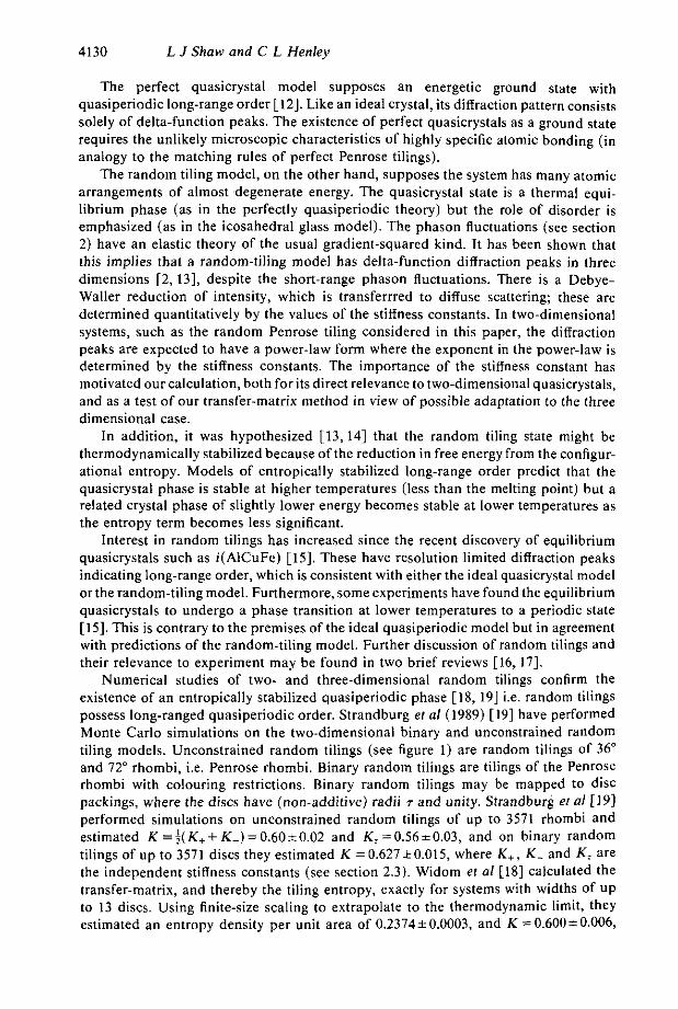
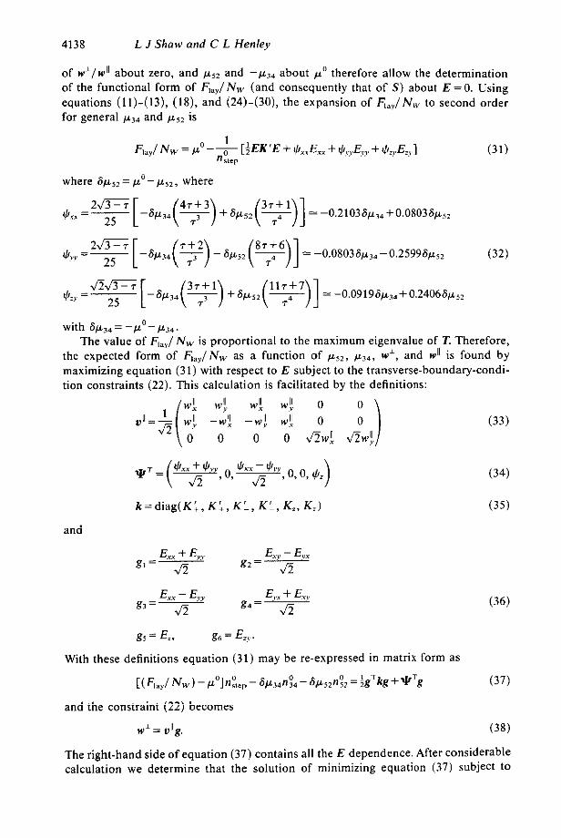
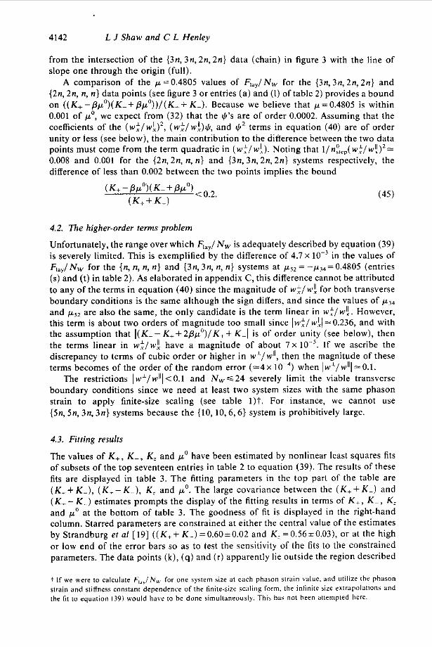
where c is a function of w' /wI I , fi34 and f i 52 . This scaling form is consistent with capillary wave theory 1251, the six-fold symmetric random tiling of the 60" rhombi (see appendix C and 1261) and the data of Widom et a/ 1181. To illustrate the smallness of the corrections to the finite-size scaling form, figure 2 displays F,,,/ Nw against N G 0'52m I3nf3n,n,nl
-3 2;' 01 ::y,,,j In,n.n.nl
0.46 0 5 10 15 20
( i / ~ " ~ ) x io3 Figure 2. Finite size behaviour of F, , , /N, for ( n . n, n. n) and (3% 3% n. nt systems for
= - F , ~ = 0.4805. The error bars of the { 3 n , 3n, n, n ) data points and the two right-hand (n, n, n, n) data points are magnified for clarity.
Transfer-matrix MC of random Penrose tiling 4141
for two systems: { n , n, n, n ) layers with n = 2 , . . , ,6 , and {3n, 3n, n, n } layers with n = 1,2,3, where pS2 = -p34 = 0.4805. Table 2 displays least-squares infinite size extrapolations of the TMMC data using equation (41). The n + CO extrapolations for 1 3 4 3% 2% 2 n ) systems utilized Fl,,/Nw data from {3,3,2,2} and (6,6,4,4} systems, and the {2n, 2n, n, nl extrapolations utilized {4,4,2,2} and IS, S,4,4) systems.
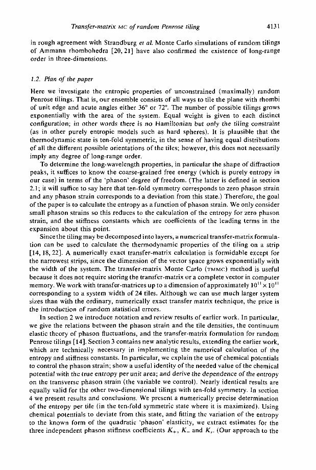
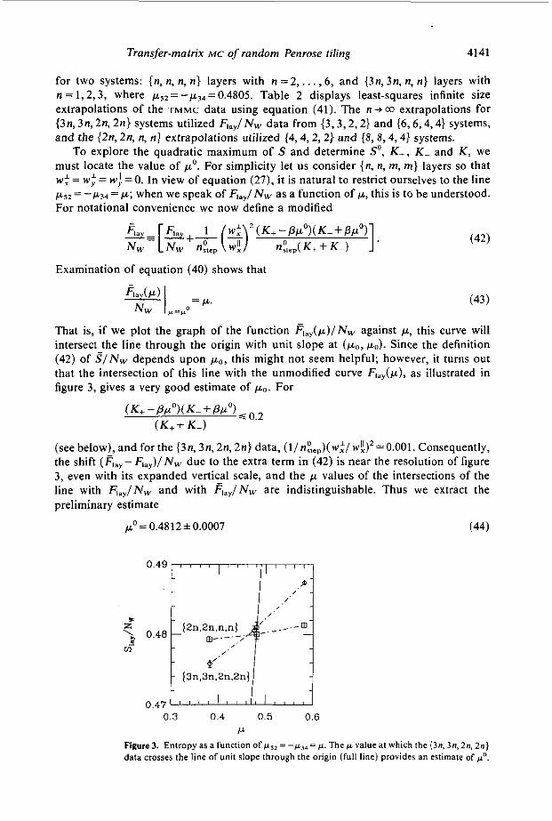
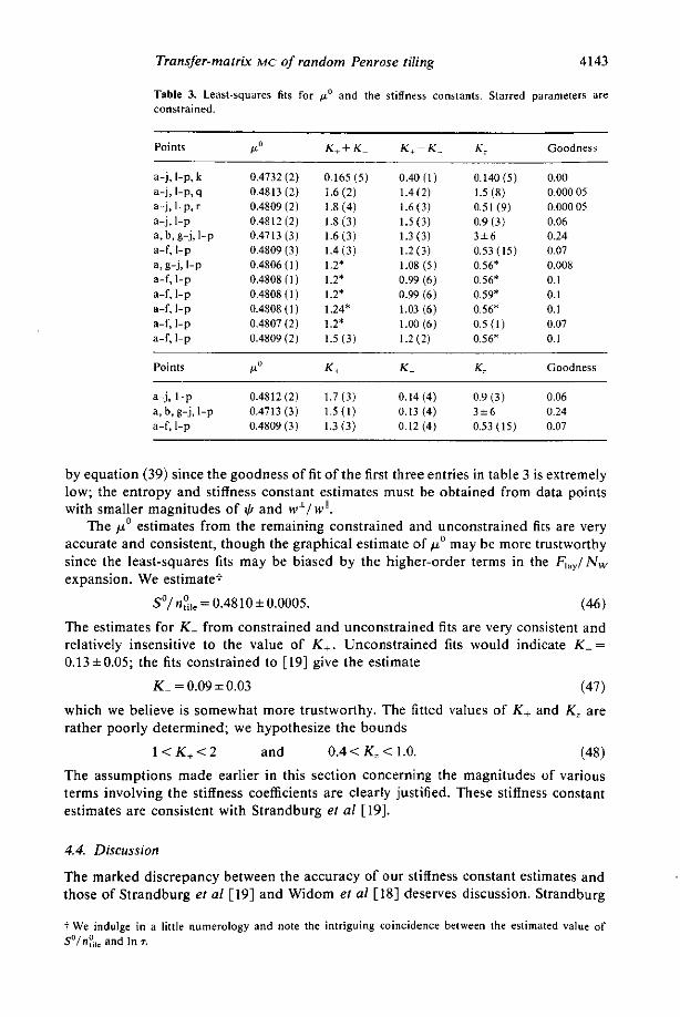
To explore the quadratic maximum of S and determine So, K , , K _ and K , we must locate the value of pa. For simplicity let us consider { n , n, m, m } layers so that w: = w: = w! = O . In view of equation (27), it is natural to restrict ourselves to the line p5> = -p3q = p; when we speak of Flay/ Nw as a function of p, this is to be understood. For notational convenience we now define a modified
Examination of equation (40) shows that
That is, if we plot the graph of the function Fkay(p) /NW against p, this curve will intersect the line through the origin with unit slope at (po, pO). Since the definition (42) of S I N w depends upon po, this might not seem helpful; however, it turns out that the intersection of this line with the unmodified curve F,&), as illustrated in figure 3, gives a very good estimate of pLo. For
( K + - Pw0)(K- +Pro) ~ o,2 ( K + + K - )
(see below), and forthe (3n, 3n, 2n, 2 n ) data, ( l /np , , , ) (w: /wL)2=0.001. Consequently, the shift (F,ay- Flsy)/Nw due to the extra term in (42) is near the resolution of figure 3, even with its expanded vertical scale, and the p values of the intersections of the line with Fl.,/Nw and with Flilny/NW are indistinguishable. Thus we extract the preliminary estimate
po=0.4812f0.0007 (44)
0.47 0.3 0.4 0.5 0.6
P Figure% Entropyasa functionofps,=-p',n=p.Thepvalueatwhich the (3n ,3n ,2n32n) data ccosses the line of unit slope through the origin (full line) provides an estimate of p".
4142 L J Shaw and C L Henley
from the intersection of the {3n, 3n, 2n, 2n) data (chain) in figure 3 with the line of slope one through the origin (full).
A comparison of the p=O.4805 values of Ft , , /Nw for the {3n,3n,2n,2n} and ( 2 4 2n, n, n} data points (see figure 3 or entries (a) and ( I ) of table 2) provides a bound on ( ( K , - P p ' ) ( K _ + P p O ) ) / ( K , . + K) . Because we believe that p=0.4805 is within 0.001 of po, we expect from (32) that the $'s are of order 0.0002. Assuming that the coefficients of the ( W : / W ! ) ~ , ( w ; / w ! ) $ , and IL2 terms in equation (40) are of order unity or iess (see beiowj, the main contribution to the difference between the two data points must come from the term quadratic in ( w $ / w ! ) . Noting that l / n ; , . J w $ / ~ ! ) ~ = 0.008 and 0.001 for the {2n, 2n, n, n } and {3n, 3n, 2n, 2n) systems respectively, the difference of less than 0.002 between the two points implies the bound
4.2. The higher-order terms problem
Unfortunately, the range over which F,,,/ N , is adequately described by equation (39) is severely limited. This is exemplified by the difference of 4.7 x IO-' in the values of Ft.,/Nw for the {n, n, n, n } and {3n,3n, n, n} systems at + s 2 = - ~ ~ ~ = 0 . 4 8 0 5 (entries (s) and (t) in table 2). As elaborated in appendix C , this difference cannot be attributed to any of the terms in equation (40) since the magnitude of w $ / w ! for both transverse boundary conditions is the same although the sign differs, and since the values of pjq and p S 2 are also the same, the only candidate is the term linear in w : / w ! . However, this term is about two orders of magnitude too small since Iw:/ w.!i = 0.236, and with the assumption that I (K_-K++2Ppn) /K,+K-I is of order unity (see below), then the terms linear in w ; / w ! have a magnitude of about 7 x IO-'. If we ascribe the discrepancy to terms of cubic order or higher in w'/w", then the magnitude of these terms becomes of the order of the random error (=4 x
The restrictions I w'/wl'l< 0.1 and Nw s 2 4 severely limit the viable transverse boundary conditions since we need at least two system sizes with the same phason strain to apply finite-size scaling (see table I )? . For instance, we cannot use {5n, 5n, 3n, 3n) systems because the {IO, IO, 6,6} system is prohibitively large.
when 1 w'/ will = 0.1.
4.3. Fitting results
The values of K,, K - , K: and ,U" have been estimated by nonlinear least squares fits of subsets of the top seventeen entries in table 2 to equation (39). The results of these fits are displayed in table 3. The fitting parameters in the top part of the table are (K++ K - ) , ( K , - K ) , Ki and p'. The large covariance between the ( K , + K - ) and ( K + - K - ) estimates prompts the display of the fitting results in terms of K,, K - , Kz and p" at the bottom of table 3. The goodness of fit is displayed in the right-hand column. Starred parameters are constrained at either the central value of the estimates by Strandburg eta1 [I91 ( ( K + + K _ ) = 0 . 6 0 + 0 . 0 2 and KI=0 .56+0 .03) , or at the high or iow end of the error bars so as to iest the sensiiiviiy OT ihe fiis io iiie coiisiiaiiied parameters. The data points (k), (4) and (I) apparently lie outside the region described
? I f we were to calculaie F,,,,/ N,, roc one ryrrem size at each philsan strnin Y B I U C . and utilize rhe phsson stmin and stiffness canstani dependence of the finite-size scaling form. the infinire iize rrtrapalations and the 61 to equation 139) would have to be done aimullaneously. This has not heen attempted here.
Transfer-matrix M C of random Penrose tiling
Table 3. Least-squares fits for constrained.
4143
and the stiffness constants. Starred parameters are
Points F 0 K + + K - K + - K . KT Goodness
a-j, I-p, k a-]. I - P , ~ a-j, I-p, I a-j, I-p a, b, g-j, 1-P a-f, I-p a,g-J, I - P a-f, I-p a-f. I-p a-f. I-p a-f, I-p a-f, I-p
0.4732 (2) 0.4813 (2) 0.4809 (2) 0.4812 (2) 0.4713 (3)
0.4806 (I) 0.4808 ( I )
0.4808 ( I ) 0.4807 (2) 0.4809 (2)
0.4809 (3)
0.4808 ( 1 1
0.165 (5) 0.40 (1) i . 6 (2) 1.4(2) 1.8 (4) 1.6 (3) 1 .8(3) 1.5(3) 1.6 (3) 1 . 3 (3) 1.4 (3) 1.2 (31 l.2* 1.08 (51 1.2* 0.99 (6) 1.2* 0.99 ( 6 ) 1.24* 1.03 (6) 1.2* 1.00 ( 6 )
0.140 (5) 1.5 (8) 0.51 (9) 0.9 (3) 3 + 6 0.53 ( I S ) 0.56* 0.56: 0.59" 0.56' 0 . 5 ( 1 ) 0.56'
0.00 0.000 05 0.000 05 0.06 0.24
0.008 0.1 0.1 0.1 0.07 0.1
0.07
Points 2 K + K . K ; Goodness
a-j, I-p 0.4812(2) 1.7 (3) 0.14 (4) 0.9 (3) 0.06 a ,b ,g - j , l -p 0.4713(3) I .5 (1 ) 0.13 (4) 3 + 6 0.24 a-f, I-p 0.4809 (3) 1.3 (3) 0.12 (4) 0.53 ( I S ) 0.07
by equation (39) since the goodness of fit of the first three entries in table 3 is extremely low; the entropy and stiffness constant estimates must be obtained from data points with smaller magnitudes of $ and w'/ W ' I .
The po estimates from the remaining constrained and unconstrained fits are very accurate and consistent, though the graphical estimate of po may be more trustworthy since the least-squares fits may be biased by the higher-order terms in the F,,,/N, expansion. We estimatet
S 0 / n ~ , . = 0.4810*0.0005. (46) The estimates for K- from constrained and unconstrained fits are very consistent and relatively insensitive to the value of K,. Unconstrained fits would indicate K _ = 0.13*0.05; the fits constrained to [19] give the estimate
(47) K - = 0.09 * 0.03
which we believe is somewhat more trustworthy. The fitted values of K, and K , are rather poorly determined; we hypothesize the bounds
(48) 1 < K + < 2 and 0.4 < K= < 1.0.
The assumptions made earlier in this section concerning the magnitudes of various terms involving the stiffness coefficients are clearly justified. These stiffness constant estimates are consistent with Strandburg el a1 [ 191.
4.4. Discussion
The marked discrepancy between the accuracy of our stiffness constant estimates and those of Strandburg e f a1 [I91 and Widom e f a1 [18] deserves discussion. Strandburg
t We indulge in a little numerology and note the intriguing coincidence between the estimated value of So/n:r,, and In i.
4144
et a1 determined the stiffness constants by measuring the phason fluctuations of a Monte Carlo simulation. This is more direct than our approach where the stiffness constants are extracted by fitting the data to equation (39). Fitting for the stiffness constants, which are the coefficients of quadratic terms in $ and w'/wIl , is difficult for noisy data because in effect it requires performing two numerical differentiations.
In [18] an entropy estimate was obtained for the constrained binary tiling with an accuracy comparable to that found here, but a much more accurate determination of the stiiiness constant iC = f(K++ E(_) was made. They caicuiated the entropy using the transfer-matrix for a series of small systems whose transverse boundary conditions minimized the phason strain. The curvature of the entropy function for these small systems was determined from the response of the entropy to varying a chemical potential. The results were extrapolated to the infinite size limit. The unexpectedly small region about E = O to which equation (39) applies makes the fit for the stiffness
accuracy of the TMMC data. It may be more fruitful to follow [IS] and calculate the second derivatives with respect to & and fiZ." for a similar set of small systems (in particular the [F", F,, Fn-,, F,-,} systems, where F, is the nth Fibonacci number), and then extrapolate to the infinite size limit. Although this may allow accurate determination of ( K + + K _ ) and K , (see equation (4011, ( K + - K - ) could not be
In conclusion, we have described a way to implement a TMMC computation of the entropy of a random Penrose tiling near zero phason strain. We have determined estimates of the maximum entropy density So and the stiffness constants K , , K - and K , . We have compared the efficacy of this computation to related Monte Carlo and finite-size transfer-matrix computations. We present for the first time an estimate of So, znd ixdependen! es!itxtes of K , 2nd K , for the random Penrose ti!ing.
L J Shaw and C L Henley
coiijiafliS, w;iic:i is in efieci equiva;ei-lt io nur,,r,icai ;ifereniia(ion, &R,cuii given iht:
""*:...-A"> L.. hL:" ,a..l...: CJLIIIIaLG" " J L l l l J r r c r r l l r q u c .
Acknowledgments
U S was supported by the National Science Foundation through the Cornell Material Science Center, and CLH was supported by the US Department of Energy grant DE-FG02-89ER45405; the computation was done in part with the support of the Cornell National Supercomputing Facility. We are grateful for many helpful discussions to M Peter Nightingale, Michael Widom, and especially Veit Elser, who also provided detailed comments on the manuscript.
Note added. A more thorough discussion of thermodynamics including the use of chemical potenlialr, and - - -"#I-* A:"" :..- ^C .L^ ^C ..*.."e.._ "~~ :- " I,~.,, ..."_..* ,.,*,I, .Ln
,",,IC p"",,c, ",JI",,l"ll "I ,us L C L I I I I I C O I I I I L O "I L l " l l D I C l .11 ..,, l.Iclll ..".- "l. .... diagram of the randam eight-fold rhombus tiling [27].
Appendix A. The transfer-matrix Monte Carlo method
A.1. Basic theory
The transfer-matrix Monte Carlo (TMMC) method [28] is a stochastic technique for doing matrix multiplications without storing the matrices or even the vectors. This makes TMMC useful for calculations involving extremely large matrices. Here we will describe the algorithm for calculating the leading eigenvalue of a matrix with non- negative entries.
Transfer-matrix MC of random Penrose riling 4145
In the transfer-matrix Monte Carlo method [28] a population of M walkers labelled with the integers {a,, a2,. . ., a,] and the positive real numbers (w, , w2,. . .. wMM) represents the n-component vector
M
U = E we,, (49) ,=, where ex is the unit vector with a single non-zero entry in the kth position, and 1 S a, S n. The a's and w's are said to represent the 'positions' and 'weights' of the walkers respectively.
TMMC multiplication of v by the transfer-matrix T is accomplished by performing a 'TMMC decomposition' of T into the product of a diagonal matrix D and a stochastic matrix P, i.e. T = PD. where, by definition, the sum of the entries in each column of a stochastic matrix is unity. Assume that all the entries of T are positive, then all the entries of P and D can also be positive, and the entries of P may be interpreted as probabilities. Upon the operation of P on the population representing U, the position a, of each walker has the probability P,:,,, of changing to a:, The weights are unchanged by P. On average, the vector equivalent (as in equation (49)) of the resulting population is equal to Pu. As M + m, the vector equivalent of the TMMC operation of P on D
becomes equal to the matrix multiplication Pv. The matrix D operates on U by changing theweights{w,, w2,. . . , w,}of U to{D,,,,,w,, Do2,y2w2,. . . , D,,,,,w,},whileleaving the positions unchanged. Clearly the vector equivalent of the TMMC operation of D on U is equal to Do. If the weights of the population representing U are non-negative, the weights of T"u are also non-negative.
On repeated application of P and D to the population, some walkers will accrue very large weights and others will accrue very small weights. It is computationally advantageous to divide each of the walkers with larger weights into a number of walkers with smaller weights, and to conglomerate or annihilate walkers with very small weights. There are many algorithms for redistributing the positions and weights of the walkers while, on average, keeping the vector equivalent unchanged [28,29]. We have found the following algorithm to reduce the variance of TMMC calculations and to be computationally efficient. Before redistribution, the population weight
W = E wI/Mlargel (50) I
is factored from each walker weight w, i.e
The population weight is to be considered as a scalar prefactor to the vector equivalent of the population. If the new scaled weight of a walker satisfies the bounds f S w, < 2, the weight and position are left unchanged by redistribution. If 2 6 w,, the walker at a, is replaced by [w,] walkers at a,, each with a weight of w,/[w,l, where [XI is the greatest integer less than or equal to x. If w, <;, the walker is replaced with a walker at the same position with a weight of unity with a probability w,, and destroyed with a probability of 1 - w,. This algorithm insures that ( i ) the walker weights stay between f and 2, (ii) the number of walkers remains near M,,,,,,, and (iii) on average the vector equivalent of the population is unchanged.
The scalar prefactor of the vector equivalent of the population after T~ successive applications of the transfer-matrix and redistributions of the population, is the product
4146
of the population weights W, W, . . . WTr. When using TMMC, the natural norm of an n-dimensional vector is the I-norm: IIuII, =X:=, I u , ~ . After the T,th scalar prefactor is divided from the population weights, but before the redistribution operation,
L J Shaw and C L Henley
Estimation of the leading eigenvalue Aa of T utilizes the relation
U"= lim T'w,. (53) (."it)--
where the expansion of U,. in terms of the eigenvectors of T is required to contain a non-zero component of v o , A o , A , , A,, . . . are the eigenvalues in order of descending magnitude, [-'= ln(Aa/Al) is the correlation length, and U,= (I /A,)Tv is the leading eigenvector. The random Penrose tiling, as a critical system, has a correlation length on the order of the width of the system ( = N , ) 1301.
The leading eigenvalue A. can he extracted either using the relationship
In terms of the population weights, equations (54) and ( 5 5 ) lead to two alternative A. estimators:
and
respectively. The summation performs an average over approximately max{T,/(, T,,/T,} independent terms. The random fluctuations in the vector equivalent of the population with i+j insure that the vector equivalent of the population will generally contain a non-zero component of U,, in an expansion in terms of the eigenvec- gors of T. There are systematic and random errors associated with finite M and T,,,
but for with M'mor T , , ' W , A ~ ' ( M , T , , T ~ ) ' A ~ .
A.Z. Implementation
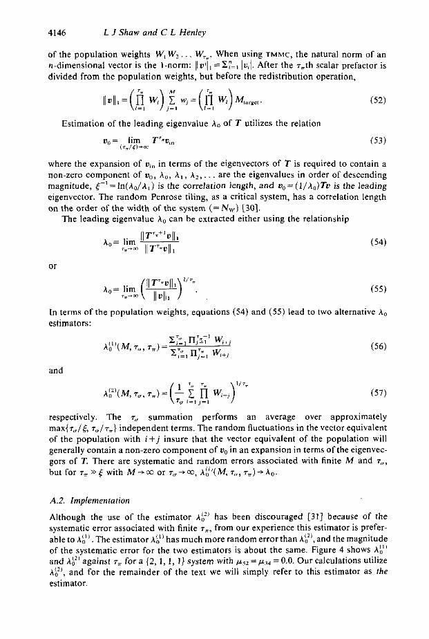
Although the use of the estimator A;' has been discouraged 1311 because of the systematic error associated with finite T,,, from our experience this estimator is prefer- able to A:". The estimator AY' has much more random error than Ag', and the magnitude of the systematic error for the two estimators is about the same. Figure 4 shows A Y ' and A;'' against T~ for a 12, 1, 1, I } system with wS2 = pj4 = 0.0. Our calculations utilize Ab,', and for the remainder of the text we will simply refer to this estimator as the estimator.
Transfer-matrix MC of random Penrose tiling 4147
0 10 20 30 40 50 T.7
~ i g u r e 4. ne estimators A:! and ,iF! from a singie run ior D ii, i , i . i j system with flS2 = 0.0, M = IO0 and i,, = 100. The broken line marks the exact leading eigenvalue.
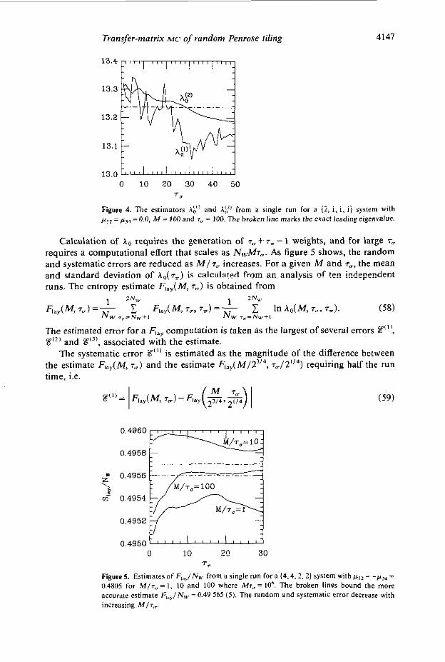
Calculation of ho requires the generation of T" + T , - 1 weights, and for large 'rr requires a computational effort that scales as NwMr,. As figure 5 shows, the random and systematic errors are reduced as M/T, increases. For a given M and T", the mean and standard deviation of A c ( ~ r ) is calculated from an ana!ysis of !en Independent runs. The entropy estimate F,,,( M , T,,) is obtained from
Flay(M,~m)=- 1 F , a y ( M , ~ c , r r ) = - 1 InA0(M,'r,,,Tr). (58)
The estimated error for a F,,, computation is taken as the largest of several errors @ ' I ,
%'(2) and 8(3', associated with the estimate. The systematic error %'"' is estimated as the magnitude of the difference between
the estimate F,,,(M, ru) and the estimate F,,,(M/Z"", T , , / Z " ~ ) requiring half the run time, i.e.
1 Z N w 1 2Nw
N w T ~ = N ~ + I Nw i ,=~w+i
0.4960
0.4958
0,4956 E . - . A X i T , = i O G
z'
M / T , = ~ B \. m- 0.4954
0.4952
B
0.4950 0 ! O 20 30
7"
Figure 5. Estimates of F,,,,/Nw from a single run for a (4.4. 2. 2) system with pS2 = -e3< = 0.4805 for M/T,,=I, 10 and 100 where Mr,,= IO*. The broken lines bound the more accurate estimate F,, , , /Nw =0.49 565 ( 5 ) . The random and systematic error decrease with increasing M / T ' , .
4148 L J Shaw and C L Henley
The random errors 8'" and 8'3' are
and
8'"= max SFl,,(M, T", 7,) (61) N w c 7 , h Z N w
where SF,,, is the standard deviation of Flay. For constant MT,,, 8'" and 8"' are relatively insensitive to N,; but 8"' grows rapidly (probably exponentially) with N,. To obtain entropy estimates with an accuracy of about 0.1% or less we are restricted to system sizes Nw s 24. The errors 8"' and 8'3) are typically of the same order of magnitude for those system sizes under consideration here.
To illustrate the typical parameters for a data point calculation we present two examples. The calculation of FLayl N , to an accuracy of 0.01% for the {4,4,2,2} system with pS2 = - w , ~ = 0.4805 was achieved by a run with M = 20 496 and T* = 142, requiring 4.1 CPU hours on a Convex C210. The magnitudes of the errors were 8'" = 3.7 x 8"' = 2 x For the {6,6,3,3} system with psz = -p3,= 0.4805, an accuracy of 0.06% was achieved by a run with M = 20 489 and = 142 requiring seven CPU hours on the Convex. The magnitudes of the errors were 8"' = 3.1 x 8'" = 2 x
and go' = 4.9 x
and 8'" = 6 . 2 , ~ lo-'.
Appendix B. TMMC for the random Penrose tiling and importance sampling
B.1. TMMC implementation of the tiling rules
The tiling rules and the TMMC method have been described in section 2.4 and appendix A, respectively. This section outlines the algorithm for a TMMC implementation of the tiling rules to compute the entropy of the tiling.
The entropy is computed by monitoring the population weight while repeatedly applying the transfer-matrix T = TssTsLTLr to the walkers. The diagonal operators of the TMMC decompositions of T,,, TsL and TLL, modify the weights of the walkers. The stochastic operators change the positions of the walkers, the position of a walker corresponding to a configuration of steps across a layer of the tiling.
The population weight is monitored after each application of the SS rule in the course of redistributing the walkers as described in appendix A. We have found that the point within the SS-SL-LL cycle at which the redistribution is implemented has little effect on the statistics of the estimate.
The Tss, TsL and TLL algorithms described in sections B.l.1-B.1.3 (i) perform the D operation by determining the sum of the weights of all possible step permutations consistent with the tiling rules and, increasing the walker weight by this factor, (ii) perform the P operation by stochastically choosing a new step configuration with a probability proportional to the weight of that configuration.
B.1.I. The Tss operation. The string of steps is searched for all adjacent S'S- pairs (with the St on the left). Since the tiling has periodic boundary conditions, the sequence of steps across a layer is to be considered as periodic also. Each S'S- pair is a 'Tss operation interval.' For each StS- pair the walker weight is increased by a factor of (1 + z3J. where z3g = e-''". Each S'S- pair is switched to a S-S' pair with probability
Transfer-matrix MC of random Penrose tiling 4149
z3&/(1 +zj4), and left unchanged with a probability 1/(1+ z3J. The TMMC operations for each Tss operation interval are independent i.e. Pss and Dss may be decomposed into a direct product of matrices acting on individual S'S- pairs.
8.1.2. The T,, operation. The string of steps is divided into 'TSL operation intervals'. The left-hand end of each operation interval starts with an St or immediately to the right of an S-; the right-hand end of each interval ends with an S- or immediately to the left of an St. The interior of the interval consists entirely of L steps. €or example, the layer of steps [L'L-S'L'L'S'L-S-L'L-S-} consists of the TSL operation intervals [S+LtLtl, [S+L-S-], [L+L-S-], and [L+L-]. The TMMC operations for each SL interval are independent i.e. PSL and Dsr may be decomposed into a direct product of matrices acting on individual SL intervals. The application of the SL rules to the four different types of T,, operation intervals are as follows:
(i) The interval [ S + L , L , . . . L,_,L.] becomes [L ,L , L,_,S+L ,... L,_,L,],where Os is n, with probability l / ( n + l ) . The weight is increased by a factor of ( n + 1).
(ii) The interval [ L , L 2 . . . L,_,L,S-] becomes [L,L, L,KL,+, . . . L,_,L.], where 0 s is n, with probability l / ( n + 1). The weight is increa by a factor of ( n + 1).
(iii) The interval [ S t L , L 2 . . . L,,S-] becomes [ L , L,s+L,+, . . . L,s-L,+, ... L.], where 0 s i s j s n, with probability 2/[(n + l ) (n + 2)J. The weight is increased by a factor of ( n + l ) ( n + 2 ) / 2 .
(iv) The interval [ L , L 2 . . . L,_,L.] and the weight remain unchanged.
8.1.3. The TLL operation. Strings of consecutive L steps are the 'TLL operation inter- vals'. The TLL operations for each operation interval are independent, i.e. PLL and DLL may be decomposed into a direct product of matrices acting on individual TLL operation intervals.
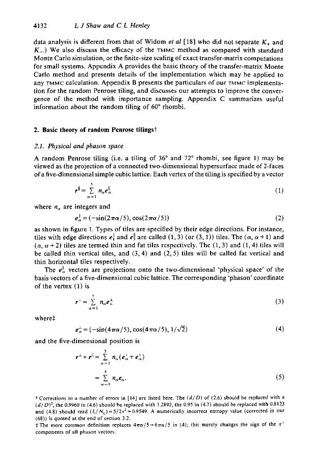
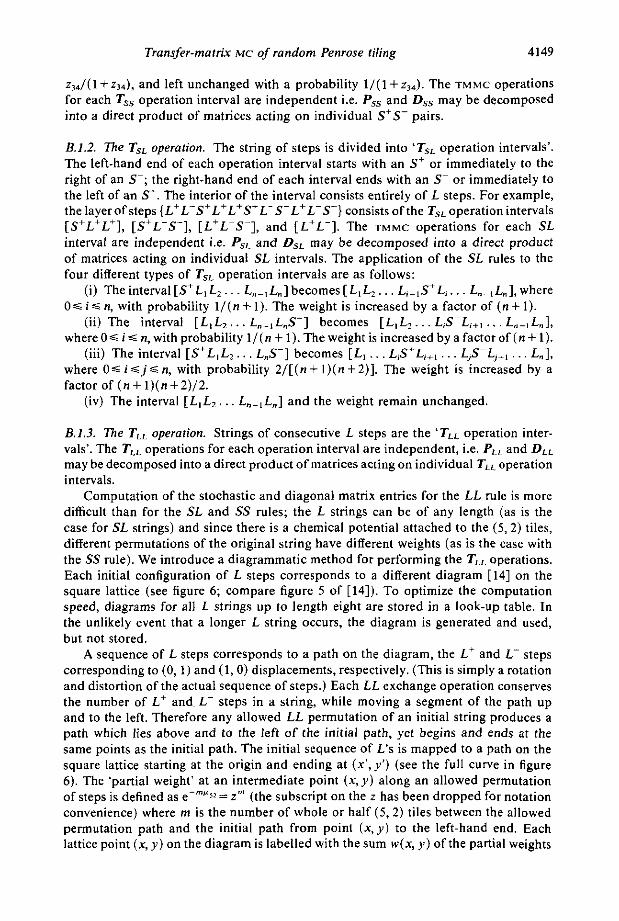
Computation of the stochastic and diagonal matrix entries for the LL rule is more difficult than for the SL and SS rules; the L strings can be of any length (as is the case for SL strings) and since there is a chemical potential attached to the (5 ,2 ) tiles, different permutations of the original string have different weights (as is the case with the SS rule). We introduce a diagrammatic method for performing the TLL operations. Each initial configuration of L steps corresponds to a different diagram [ 141 on the square lattice (see figure 6; compare figure 5 of [14]). To optimize the computation speed, diagrams for all L strings up to length eight are stored in a look-up table. In the unlikely event that a longer L string occurs, the diagram is generated and used, but not stored.
A sequence of L steps corresponds to a path on the diagram, the Lt and L- steps corresponding to ( 0 , l ) and (1,O) displacements, respectively. (This is simply a rotation and distortion of the actual sequence of steps.) Each LL exchange operation conserves the number of L' and L- steps in a string, while moving a segment of the path up and to the left. Therefore any allowed LL permutation of an initial string produces a path which lies above and to the left of the initial path, yet begins and ends at the same points as the initial path. The initial sequence of L's is mapped to a path on the square lattice starting at the origin and ending at ( x ' , y ' ) (see the full curve in figure 6 ) . The 'partial weight' at an intermediate point (x,y) along an allowed permutation of steps is defined as e-'"'52= 2"' (the subscript on the L has been dropped for notation convenience) where m is the number of whole or half ( 5 . 2 ) tiles between the allowed permutation path and the initial path from point (x, y ) to the left-hand end. Each lattice point (x, y) on the diagram is labelled with the sum w ( x , y ) of the partial weights
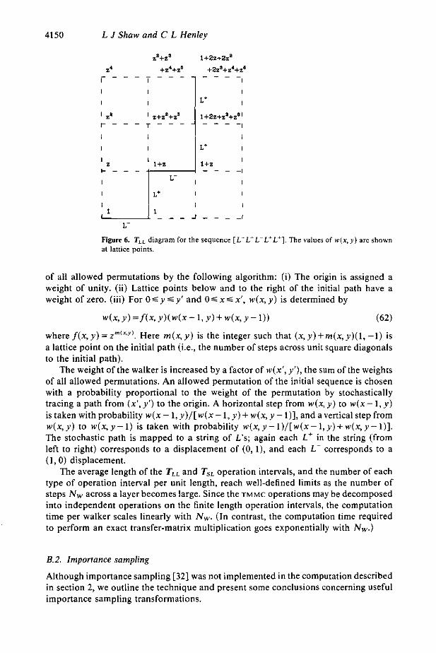
4150 L J Shaw and C L Henley
z = + 2 1+2Z+Z2
z' +z'+# + ~ ~ 3 + ~ 4 + ~ *
I
I lL:--- I
r - - - - - - - I
I I
I I
' Z+ZU+Z" 1+22+z*+2 r - - - r - - - - - - I 2 -I -I
Figure 6. T,, diagram far the sequence [L-L+L-L+L+]. The values of w ( x , y ) are shown at lattice points.
of all allowed permutations by the following algorithm: (i) The origin is assigned a weight of unity. (ii) Lattice points below and to the right of the initial path have a weight of zero. (iii) For O s y s y ' and OS x s x', w ( x , y ) is determined by
W ( X , Y ) = f ( X . Y ) ( w ( x - 1 , Y ) + w w ( X , Y - 1 ) ) (62)
wheref(x,y)=z"'"~'". Here m ( x , y ) is the integer such that ( x , y ) + m ( x , y ) ( l , - 1 ) is a lattice point on the initial path (i.e., the number of steps across unit square diagonals to the initial path).
The weight of the walker is increased by a factor of w ( x ' , y ' ) , the sum of the weights of all allowed permutations. An allowed permutation of the initial sequence is chosen with a probability proportional to the weight of the permutation by stochastically tracing a path from (x', y ' ) to the origin. A horizontal step from w ( x , y ) to w ( x - 1, y ) istaken withprobability w(x-1,y)/[w(x-1,y)+w(x,y-1)],andaverticalstepfrom w ( x , y ) to w ( x . y - 1) is taken with probability w ( x , y - l ) / [ w ( x - I , y ) + w ( x , y - l ) ] . The stochastic path is mapped to a string of L's; again each L+ in the string (from left to right) corresponds to a displacement of (0, l ) , and each L- corresponds to a (1,O) displacement.
The average length of the TLL and TSL operation intervals, and the number of each type of operation interval per unit length, reach well-defined limits as the number of steps N , across a layer becomes large. Since the TMMC operations may he decomposed into independent operations on the finite length operation intervals, the computation time per walker scales linearly with Nw. (In contrast, the computation time required to perform an exact transfer-matrix multiplication goes exponentially with N w . )
8.2. Importance sampling
Although importance sampling [32] was not implemented in the computation described in section 2, we outline the technique and present some conclusions concerning useful importance sampling transformations.
Transfer-matrix MC of random Penrose tiling 4151
By the weighting algorithms outlined in this appendix, and equations (50) and (57), the variance of TMMC estimates vanishes when each of the diagonal matrices Dss, DSL and D,,, is proportional to the identity matrix. An effective importance sampling implementation performs a transformation on the transfer-matrices which makes the diagonal matrices more nearly proportional to the identity matrix, thereby reducing the variance of the estimates, while leaving the eigenvalue spectrum unchanged.
For simplicity we consider a transfer-matrix T = TI T2 ( T , and T2 are arbitrary), where U, and u2 are the leading left eigenvections of T,T2 and T,T, respectively, i.e.
u , T , T 2 = A,u, and u,T,T, = Aou2. (63)
~ U , T , U ; ' = U , T , U ; ' = A , U ~ U ; ' = A , I (64) IU2T,U;'=u2T2U;'=h,u,U;'=A,l (65)
where entries of the vector 1 are all unity, and U, = diag(u,). The vector 1 is the leading left eigenvector of T f = U2T,U;' and TT = U, TI U ; ' , and therefore the diagonal parts of the TMMC decompositions of T: and TT are proportional to the identity matrix. Since T, T2 is related to
(66) by a similarity transformation, the eigenvalues of both products are the same. Matrices of the form VT,W-' and VT,W-', where V and W are any diagonal matrices, are said to be the importance sampled versions of T , and T2.
Unfortunately, if we are using TMMC to determine the leading eigenvalue, the leading left eigenvectors are certainly not known. Effective importance sampling relies on finding vectors which (i) are a good approximation to the leading left eigenvectors, and (ii) are of a form such that the speed of the TMMC operations is not greatly reduced.
It is crucial that the importance sampling transformed matrices may be decomposed into direct products. Otherwise the advantages mentioned at the end of section B.l are lost since a stochastic operation consists of a single random choice among all possible tiling permutations (a daunting prospect considering that the number of permutations grows exponentially with the system width while the weighting of each permutation is non-trivial).
Then u , T , = u , , u,T,=u,,and
TTTT = ( U , T , u ; ~ ) ( u ~ T ~ u ; ~ )
Consider the TMMC application of some importance sampled matrix T*,
(67) where V and W are any two diagonal matrices, and P*D* and P*D** are the TMMC
decompositions of T* and W, respectively. Useful forms of W-' do not have to have the same operation intervals as D** if we choose to apply W-' and D** sequentially. (Sequential application of these operations is equivalent to the application of their product since the matrices are diagonal and TMMC algorithm does not involve any random choices.) On the other hand, application of VT is not equivalent to sequential application of the two TMMC operations since the stochastic matrices of the TMMC
decompositions of T and W are different. For VT to maintain the same operation intervals as T, (i) the functional form of the entry V,, must be a product of n factors, where n is the number of T operation intervals in the ith configuration, and (ii) only a single factor in the product must change on application of the T operations to a single operation interval. It is not clear whether there are useful importance sampling transformations for the tiling which saitisfy the above restrictions.
T* = VTW-'= p*D** W-1= p*D*
4152 L J Show and C L Henley
Appendix C . Application of 60-degree rhombus tiling
The 60" rhombus tiling is a non-quasicrystalline analogue of the Penrose tiling with a one-dimensional 'phason' space. The 60" rhombus tiles have edge vectors
d, = (-sin(2?ra/3), c o s ( Z ~ a / 3 ) )
",." - *A . I P l t ; , . e L ....L.-ua of a ~ ! i n g are by p=, E&m. ;he :ile densZe; for type of tile are equal, the entropy per tile is [33]
=0.323 066. (68)
A distortion of the tiling plane maps a 60" rhombus tiling onto a special case of the Penrose tiling using only three out of the ten types of rhombi. The mapping
d, + er d2+ -e4 I/ d , + - e l
transforms a 60" rhombus tiling to a tiling of the (1,3), (1,4) and (3,4) Penrose tiles. When n , , = rill= n,4, the average area per tile is -0.7088; dividing the entropy in (68) by this figure, the entropy per unit area is 20.4558. Similarly, mapping
produces a tiling of the (1, 2 ) , (1,5) and ( 2 , 5 ) Penrose tiles. When q2= n I 5 = n25r the average area per tile is =0.8300, and the entropy per unit area is =0.3893.
A comparison of the above exact values of the entropy density for special cases of the phason strain, with estimates produced using the results of section 4.1 and equation (16), confirms that there are significant corrections to the quadratic form assumed in equation (15). A random tiling of equal densities of (1 ,3) , (1,4) and (3 ,4) tiles has an entropy density of -0.46 and non-zero phason strain components E, = 7 and Eyy = T - ~ . But, since K , is at least as large as unity and the entropy density maximum So has a value of about 0.59, the entropy density according to equation (16) should be considerably negative (about -2) with this phason strain. A similar analysis for the random tiling with equal densities of (1, 2 ) , (1 ,s) and (2,5) tiles (non-zero phason strain components E, = T - ' , E,">, = T - ~ and E,, = 2~'?7-~, and entropy density ~ 0 . 3 9 ) shows that the entropy density according to equation (16) should again be negative (5-0.3).
References
[ I ] Shechtman D S. Blech I , Gratias D and Cahn J W 1984 Phyr. Reo. Lerr. 53 1951 [2] Henley C L 1987 Commenr Condenr. Maller Phys. 13 59 [3] Jarif M V (ed) 1988 Apcriodieiry and order, 001 1: lnrroducrion IO Qunsicryrrolr (Boston: Academic) [4] JariC M V and Gratiar D (ed) 1989 Aperiodiciry and order, uol 3: Exrended Icosohedrol Srrucrures
(Boston: Academic) r e ? ,I^__ " . I ."^,.1.11. I./ -:<,:... --. .. n ..- ̂̂ ^_ I ,.__I os...,.:-- 0 "L... ".., ,-., =I( ,""" L,, " " # I t r 111. LwIaILIcIYL n, "l"l l lLC"L" " r, I " 1 1 S I .I .,,I" U C t I I I U I I I " R li.0" ""A. me". L C I , . > I I...t?
[6] Baiicel P A, Heiney P A , Stephens P W, Goldman A I and Horn P M 1985 Phy,t. R e v Lelr. 54 2422 [7] Shechtman D S a n d Blech I 1985 Merallurg. Tronr. A 16 IOOS [8] Stephens P W and Goldman A I 1986 Phys. Reo. Lelr. 56 1168 [9] Stephens P W 1989 Aperiodiri1.v and order, "01 3: Exrended leosahedrol Slrucrurer ed M V JariC and
[IO] Elser V 1987 h o c . XVrh lnrernorional Colloquium o;l Group Theory in Physics ed R Gilmore and D H D Gratiar (Boston: Academic) pp37-104
Feng (Singapore: World Scientific)
Transfer-matrix MC of random Penrose tiling 4153
[I I ] Elser V 1989 Aperiodicily and order, "013: Extended Icosohedrnl Structures ed V Jarit and D Gratias
[I21 Levine D and Steinhard1 P J 1984 Phyx. Rev B 53 2477 1131 Eiser V 1985 Phys. Rev. Lerr. 54 1730 1141 Henley C L 1988 J. Phys. A : Moth. Gen. 21 1649 1151 Bancel P A 1989 Phys. Reo. Lell. 63 2741 [I61 Henley C L 1990 Quasicrysrals and lncommenrurole Srruerures in Condensed Marrer ed M J Yacamsn,
[17! Widom M 1990 Ounricry~rols ed M V JariC and S Lundqvist (Singapore: World Scientific) [IS] Widom M, Deng D P and Henley C L 1989 Phys. Res. L e n 63 310 1191 Strandburg K J, Tang L-H and JariC M V 1989 Phys Re". Let!. 63 314 1201 Tang L-H 1990 Phys Rev. Lerr. 64 2390 I211 Shaw L J . Elser V and Henley C L 1991 Phys. Re". B 43 3423 [22] Kawamura H 1983 Prog. Theor. Phys. 70 697 1231 Bak P 1985 Phyr Re". B 32 5764 1241 Lubensky T C 1988 Aperiadiciry and order. vol I : Introduction to Quasieryslolr ed M V Jarii- (Boston:
1251 Gelfand M P and Fisher M E 1988 In!. J. Thermophys. 9 713 1261 Li W, Park H and Widom M 1990 1. Phys. A: Moth. Gen. 23 L573 [27] Li W, Widom M and Park H 1991 J. Slal. Phys. in press [28] Hetherington J H 1984 Phys. Re". A 30 2713 1291 Nightingale M P 1988 Proc. 3rd Inl. Con! Supercomputing I (Boston, MA) ed L P Kartashev and S I
[ X j Nightingsie ivi P I976 Physiro 8 3 5 6 i [31] Nightingale M P and Bliite H W J 1986 Phys. Rev. B 33 659 1321 Nightingale M P 1990 Finire-Size Sealing ond Numerical Simularion of Storisricol Sysrems ed V Privman
Nightingale M P and Catlisch R G 1988 Computer Simulorion Studies in Condensed M a l m PhyJicr ed
(Barton: Academic) pp 105-36
D Romeu, V Castario and A G6mez (Singapore: World Scientific) p 152
Academic)
Kanashev
(Singapore: World Scientific) p 287
D P Landau and H B Schiittler (Berlin: Springer) 1331 WannierG H 1950 Phys. Rev. 79 357; 1973 Phys. Rev. B 7 5017 (E)