a time series model of interest rates with the effective ... · a time series model of interest...

Finance and Economics Discussion SeriesDivisions of Research & Statistics and Monetary Affairs

Federal Reserve Board, Washington, D.C.

A Time Series Model of Interest Rates With the Effective LowerBound

Benjamin K. Johannsen and Elmar Mertens

2016-033

Please cite this paper as:Johannsen, Benjamin K., and Elmar Mertens (2016). “A Time Series Model of In-terest Rates With the Effective Lower Bound,” Finance and Economics DiscussionSeries 2016-033. Washington: Board of Governors of the Federal Reserve System,http://dx.doi.org/10.17016/FEDS.2016.033.

NOTE: Staff working papers in the Finance and Economics Discussion Series (FEDS) are preliminarymaterials circulated to stimulate discussion and critical comment. The analysis and conclusions set forthare those of the authors and do not indicate concurrence by other members of the research staff or theBoard of Governors. References in publications to the Finance and Economics Discussion Series (other thanacknowledgement) should be cleared with the author(s) to protect the tentative character of these papers.

A Time Series Model of Interest Rates With theEffective Lower Bound

Benjamin K. Johannsen∗

Federal Reserve BoardElmar Mertens

Federal Reserve Board

April 4, 2016

Abstract

Modeling interest rates over samples that include the Great Recession requires taking stockof the effective lower bound (ELB) on nominal interest rates. We propose a flexible time–series approach which includes a “shadow rate”—a notional rate that is less than the ELBduring the period in which the bound is binding—without imposing no–arbitrage assumptions.The approach allows us to estimate the behavior of trend real rates as well as expected futureinterest rates in recent years.

∗For correspondence: Benjamin K. Johannsen, Board of Governors of the Federal Reserve System, WashingtonD.C. 20551. email [email protected]. Tel.: +(202) 530 6221. We would like to thank seminarand conference participants at the Federal Reserve Banks of Cleveland and Richmond, the Federal Reserve Board, theUniversity of Texas at Austin, the World Congress of the Econometric Society (2015), and the Dynare Conference(2015), for their useful comments and suggestions. The views in this paper do not necessarily represent the views ofthe Federal Reserve Board, or any other person in the Federal Reserve System or the Federal Open Market Committee.Any errors or omissions should be regarded as solely those of the authors.

1

mailto:[email protected]

1 Introduction

This paper models nominal interest rates, along with other macroeconomic data, using a flexi-

ble time-series model that explicitly incorporates the effective lower bound (ELB) on nominal

interest rates. We employ a modeling device that we refer to as a “shadow rate”—the nomi-

nal interest rate that would prevail in the absence of the ELB—which is conceptually similar

to the shadow rates studied in the dynamic term–structure literature, as in Kim and Single-

ton (2011), Krippner (2013), Priebsch (2013), Ichiue and Ueno (2013), Bauer and Rudebusch

(2014), Krippner (2015), and Wu and Xia (2016). Our time–series approach allows us to es-

timate the relationship between interest rates and macroeconomic data in a flexible way and,

similar to the approach taken in Diebold and Li (2006), does not impose rigid no–arbitrage

restrictions across the term–structure of interest rates.

We use our approach to estimate a trend–cycle model of U.S. data on interest rates, un-

employment, and inflation over a sample that includes the recent spell at the ELB. Since the

global financial crisis of 2008, real interest rates have been historically low, prompting some

— for example, Summers (2014) and Rachel and Smith (2015) — to argue that the long–run

normal level of real interest has fallen. Using our estimated model, we find that the trend com-

ponent of the nominal interest rate has declined almost continuously since the early 1980s. The

decline is due to long–standing downward trajectories of the trend component of both inflation

and the real short–term interest rate. While uncertainty bands around our estimate of the trend

real rate are wide, we find that any decline since the global financial crisis of 2008 is best

characterized as a continuation of a longer term downward trajectory. Similar to Laubach and

Williams (2003, 2015), Clark and Kozicki (2005), Hamilton et al. (2015), Kiley (2015), and

Lubik and Matthes (2015) we find large uncertainty bands notwithstanding some differences

in point estimates.1 However, none of these papers explicitly models the ELB.

When we ignore the constraints imposed by the ELB on the data and proceed by applying

a standard linear–state–space version of our model, we estimate a larger decline in the trend

interest rates in recent years than in our model with the ELB. The reason is that the gap be-

1Notably, our estimated trend real rate displays less movement than the trend estimates reported by Laubach andWilliams (2003, 2015), and does not not dip as low during the recent recession.

2

tween the observed interest rates and the estimated trend is not as large as the gap between

our estimated shadow rate and the trend. Without a large cyclical movement associated with

the Great Recession, the model has an easier time explaining the prolonged period with the

short–term interest rate at the ELB as a change in trend. Additionally, explicitly modeling the

ELB has large effects on inference about out–of–sample expected short–term interest rates and

term premiums over the past several years. Our estimated shadow rates are less than the ELB

by construction, and our shadow–rate model delivers predicted paths for future short–term in-

terest rates that include extended periods at the ELB. By contrast, when we ignore the ELB,

the model predicts relatively precipitous increases in short–term rates.

We find that including a medium–term interest rate in our model—which is not constrained

by the ELB over our data sample—disciplines the behavior of the shadow rate, reflecting the

model’s estimated co–movement between yields of different maturity. Without the medium–

term yield, our shadow rate estimates would merely reflect the dynamic relationship between

short–term interest rates and the macroeconomic variables in our data set (unemployment and

inflation). However, inasmuch as medium-term rates contain useful information about the

path of expected future short–term rates, the medium-term interest rate helps us identify and

forecast the shadow rate above and beyond the information gleaned from the macroeconomic

data in our sample.

The way we incorporate the ELB and estimate the model can be extended to a broad class of

time series models. With short–term nominal interest rates at or near their ELBs in many parts

of the world, time series models that include interest rates but ignore the ELB—like a standard

vector autoregression—have been unable to adequately address the data. Moreover, reduced-

form explorations of the empirical relationship between short– and longer–term interest rates—

such as Campbell and Shiller (1991)—have often ignored the truncation in the distribution

of future short–term interest rates. Our modeling approach overcomes these shortcomings

in a wide class of otherwise conditionally–linear Gaussian state–space models. Examples

include the vector autoregressions studied in Sims (1980) and the models with time–varying

parameters studied in Primiceri (2005) and Cogley and Sargent (2005b).

Following work by Black (1995), the no–arbitrage dynamic term–structure models stud-

3

ied in Kim and Singleton (2011), Krippner (2013), Priebsch (2013), Ichiue and Ueno (2013),

Bauer and Rudebusch (2014), Krippner (2015), and Wu and Xia (2016) identify shadow rates

by imposing no–arbitrage cross–equation restrictions. These studies offer interesting insights,

yet the no–arbitrage assumptions that these authors maintain may preclude certain model fea-

tures, like stochastic model parameters. Our time series approach naturally incorporates time

variation in parameters, and thus, for some purposes—like including time–varying trends in

inflation and interest rate data or modeling stochastic volatility—offers a flexible alternative.

In addition, our shadow–rate estimates do not only reflect information embedded in a longer–

term yield but also condition on direct readings about business cycle conditions embedded in

macro variables such as the unemployment–rate gap and inflation.2

Iwata and Wu (2006), Nakajima (2011), Chan and Strachan (2014) are the closest papers in

the literature to ours. These papers also estimate time series models that incorporate the ELB.

In all of these studies, lagged observed interest rates (rather than shadow rates) are explana-

tory variables in the dynamic system. We instead allow lagged shadow rates to be explanatory

variables. In doing so we are able to more closely align our approach with the no–arbitrage

term–structure literature, and, in additional, connect the concept of the shadow rate with the

level of the short–term rate that would prevail in the absence of the ELB because we allow it to

have the same persistence and co–variance properties as short–term interest rates. Neverthe-

less, our approach is flexible enough to include both shadow rates and observed rates as lagged

explanatory variables.

2 A Model of Interest Rates and the ELB

In this section we describe our time–series model, which explicitly includes the ELB. The

model includes inflation, a short– and a medium–term nominal interest rate, and the

2In an alternative time-series approach Lombardi and Zhu (2014) use a dynamic factor model to derive estimatesof the stance of monetary policy — labeled “shadow rate” — from interest rates, monetary aggregates and variablescharacterizing the Federal Reserve’s balance sheet. However, as such, their underlying shadow–rate concept is quitedifferent from what is used here or in the dynamic term-structure literature in that their measure needs not be identicalto observed interest rates, even when the ELB is not binding, nor is their shadow rate constrained to lie below the ELBwhen the bound is binding.

4

unemployment–rate gap as measured by the CBO.

2.1 The Shadow Rate Approach

Our data set includes a short–term interest rate, which has been at the ELB during 28 quarters

in our sample. We model the interest rate (it) as the observation of a censored variable. In

particular, we assume that the nominal interest rate is the maximum of the ELB and a shadow

rate (st) so that

it = max (st, ELB) . (1)

The ELB might arise because of an arbitrage between bonds and cash, though the world has

seen negative short–term nominal interest rates in a number of countries. It also might be

thought of as a level below which monetary authorities are unwilling to push short–term in-

terest rates. For our purposes, it is taken as an exogenous known constant (which could be

made time–varying). We proceed by modeling the shadow rate, in conjunction with the other

variables in the model, using standard time–series methods, and account for the ELB when

conditioning the posterior distribution of our model on observed interest rate data.

2.2 A Time Series Model with Shadow Rates

We assume that inflation (πt), the medium–term yield (yt), and the shadow rate (st) can be

decomposed into trend and cyclical components. That is, for every data series, xt, we assume

that

xt = xt + xt where xt = limh→∞

Et (xt+h) and E(xt) = 0 (2)

The defining feature of the cyclical (gap) component, xt, is that it has a zero ergodic mean.

For the unemployment rate (ut) we assume that the gap measure derived from subtracting

the CBO’s measure of the long-run natural rate from the actual unemployment rate reflects a

detrended series akin to the xt component in (2).

5

The trend components xt are similar in spirit to the trend concept of Beveridge and Nelson

(1981); however, by treating the trends as unobserved components we allow for the conditional

expectations, Et(·) in (2), to reflect a possibly wider information set than what is known to an

econometrician at time t.3 Defining the trend components as infinite-horizon expectations

implies that changes in xt follow martingale-difference processes; and, as a result, the trend

components have unit root dynamics. As documented, for example, by Stock and Watson

(2007) and Cogley and Sargent (Forthcoming), U.S. inflation dynamics are well captured by

such a trend-cycle decomposition when trend shocks have time-varying volatility. So, for the

trend component of inflation, we write:

πt = πt−1 + σπ,tεπ,t. (3)

where επ,t ∼ N(0, 1). (Throughout the text ε·,t and η·,t indicate uncorrelated standard–normal

random variables.)

Away from the ELB, our shadow rate is identical to the short–term nominal interest rate.

We assume that the trend shadow rate has two components

st = πt + rt (4)

where rt will be our measure of the trend in real interest rates, discussed below. We assume

that rt evolves so that

rt = rt−1 + σrεr,t. (5)

To capture a connection between short– and medium–term interest rates, we assume that the

medium–term rate in our model (yt) shares a common trend with the shadow rate, adjusted

for an average term–premium.4 By assuming that yield spreads are stationary, we impose the

3See also the discussion in Mertens (forthcoming).4Specifically, the trend in the nominal medium-term yield is written as yt = st+p0 where the constant p0 represents

the average term–premium, and its estimated value reflects the average spread between medium- and short–termnominal interest rates in our sample (away from the ELB). As for all gap variables, the mean of the medium-term yieldgap, E(yt), has been normalized to zero. In principle, the distinction between shadow rates and observed nominal

6

same cointegrating relationship on nominal yields that has also been used by Campbell and

Shiller (1987) and King and Kurmann (2002). In sum, there are two stochastic trends in our

model: πt and rt.

Prior evidence suggests that shocks to trend inflation have been most likely highly het-

eroscedastic (Stock and Watson, 2007) in U.S. postwar data, possibly reflecting changes in

the anchoring of public perceptions of long–term inflation expectations and the credibility of

policymaker’s inflation goals. By contrast, the variability of the trend real rate is more likely

to reflect changes in long–term growth expectations, demographic trends and other secular

drivers (Rachel and Smith, 2015) and accounts probably only for a small share of the variabil-

ity in real rates as discussed, for example, by Hamilton et al. (2015), which cautions us against

fitting a stochastic volatility process for changes in this trend. Accordingly, shocks to trend

inflation are assumed to be affected by stochastic volatility in our model, whereas we have

chosen to specify a constant variance for the shocks to rt; in addition, both trend shocks are

supposed to be mutually uncorrelated.

We assume that the gap components of the four series in our model follow a joint autore-

gressive process. That is,

A(L)

πt

ut

st

yt

= BΣtεt (6)

whereA(L) is a polynomial in the lag operator, which has roots outside the unit circle,B is a

unit–lower–triangular matrix, and Σt is a diagonal matrix.

We include time–varying volatility in the shocks to the trend component of inflation and in

the gap–vector autoregression. We assume that σ2π,t and the diagonal elements of Σt follow a

rates could also be extended here to the nominal medium-term yield and its trend; however, in our application thedistinction would be moot since the ELB never binds for the medium-term yield in our data.

7

process given by

log(σ2j,t

)− µj = ρj

(log(σ2j,t−1

)− µj

)+ φjηj,t (7)

where σ2j,t denotes a particular diagonal element of Σt or σ2

π,t, µj is the mean of the log of the

variable j, ρj is the persistence of the process, and σj is the volatility of innovations. Stochastic

volatility helps us capture the run up in average inflation in the late 1970s and early 1980s and

gives the model flexibility to capture large changes in the gap components over the business

cycle.

Finally, we assume that observed inflation is the sum of πt, πt, and measurement error with

stochastic volatility:

πt = πt + πt + eπt , eπt = σe,tεe,t (8)

The inclusion of measurement error helps us capture highly transitory, one–off movements in

headline inflation that do not feed back into real activity.

2.3 Relationship Between Shadow and Interest Rates

We conceptualize the shadow rate as the nominal interest rate that would prevail in the absence

of the ELB. On a period–by–period basis, the interest rate is either equal to the shadow rate

or equal to the ELB. The key distinction between shadow rates and interest rates is thus that

shadow rates have unbound support.

In the model we presented in the previous section, we modeled the shadow–rate gap, as

well as its lags, as part of a joint dynamic system, which allows the shadow rate to have

the same persistence properties when the ELB is binding and when it is not. By contrast,

Iwata and Wu (2006) and Nakajima (2011) model the variables in their models as functions of

lagged observed interest rates. This means that, in those papers, at the ELB the value of the

shadow–rate in the previous period has no direct effect on its value today. This approach is

in stark contrast to the shadow–rate dynamics from dynamic term–structure literature; see, for

8

example, Wu and Xia (2016).

Similar to the term-structure literature, we embed the shadow rate into a state vector with

auto–regressive dynamics, such that the persistence of the shadow rate does not depend on

whether the ELB binds. When the ELB is binding on observed interest rates, the shadow rate is

intended to capture the hypothetical level of the nominal rate that would prevail in the absence

of the ELB constraint; accordingly, we deem it beneficial that the estimated persistence of the

shadow rate in our specification, reflects to a large degree the persistence of observed interest

rates when those are away from the ELB.

2.4 Interpretation of rt

Because interest rates are truncated shadow rates, the expected interest rate is necessarily

weakly larger than the expected shadow rate. In turn, it is also the case that,

limh→∞

Et (it+h) ≥ limh→∞

Et (st+h) = st = πt + rt. (9)

In our model, st is the median forecast of limh→∞ it+h, offering a direct connection between

far-ahead shadow rates and interest rates.5 Further, assuming that the Fisher hypothesis holds,

this connection gives rt the interpretation of the median forecast of the real interest rate in

the long run.6 Notably, the same relationship holds for the medium–term yield in our model,

up to a constant offset, because of the co-integrating relationship we have assumed. For the

remainder of the paper, we refer to rt as the trend real interest rate.

Importantly, the co-integrating relationship between the short–term interest rate and the

medium–term yield in our model allows the medium–term yield to offer direct evidence on rt.

This disciplines movements in rt because the medium–term yield is above the ELB throughout

our sample.

5In our model in section (2.2) limh→∞Et (it+h) > limh→∞Et (st+h). However, one could conceptualize modelsin which it need not be strict.

6 So long as st ≥ 0, which it is in our estimates, then our interpretation of rt applies. However, if st < 0, then themedian forecast of the limh→∞ it+h − πt+h is ELB − πt. Then rt would help determine the probability that interestrates would be above the ELB over the business cycle and would be less than the long–run median real interest rate.

9

2.5 Estimation Procedure

To estimate the parameters and unobserved states of the model, we use Bayesian methods.7

The novel modeling contribution of this paper lies in the sampling of the unobserved trend and

gap components of the data when the interest rate data are at the ELB, so we focus the text

on this step of the estimation procedure. Conditional on parameter values and a sequence of

volatilities, our model can be put into the form

ξt =Aξt−1 + Btεt (10)

Xt =Cξt (11)

it = max (st, ELB) (12)

where Xt ≡ [st, yt, πt, ut]′, εt is a vector of standard normal random variables, ξt contains

the stochastic trend and cyclical components of our model, as well as the appropriate number

of lags, the matrices A, BtTt=1, and C are constructed accordingly from the parameters and

volatilities in our model,8 and the max operator encodes the ELB in the observation equation

for the interest rate. We set the value of the ELB to zero, and assume that the federal funds rate

was at the ELB for every quarter in which the target range for the federal funds rate was 0 to

25 basis points throughout the quarter.

Our approach for drawing from the posterior of ξ ≡ [ξ1, ξ2, . . . , ξT ]′ is to first treat the

interest rate data at the ELB as missing and take draws from the posterior distribution of ξ,

which is straightforward using standard filtering and smoothing techniques. Knowing that the

interest rate is at the ELB (not simply missing) in period t amounts to knowing that the values

of ξt that are consistent with the data imply values of st that are less than the effective lower

bound during that period. Thus, we can draw from the posterior of ξ by first treating interest

rate data at the ELB as missing, and then rejecting draws until we find a ξ that is consistent

with the ELB.

Our estimation procedure is a generalization of Park et al. (2007) that applies the method-

7 Our data are quarterly, and we include two lags inA(L).8In Appendix A we show how A and C can easily be made time–varying.

10

ology of Hopke et al. (2001). Appendix A explains in further detail how to construct a draw

from the posterior distribution of ξ, conditional on the data, in a conditionally–linear Gaussian

state–space model like ours. With a draw of ξ in hand, the posterior distribution of the parame-

ters can be sampled using standard methods in the literature on conditionally–linear time series

models with time–varying parameters and stochastic volatility, such as those used in Primiceri

(2005) or Cogley and Sargent (2005b). We jointly estimate the parameters and unobserved

states of the model using Bayesian MCMC techniques; our priors and details of the MCMC

steps are described in Appendix B.

3 Shadow Rate and Trend Estimates

In this section we describe the posterior distribution of our model with regard to estimated

shadow rates and trends. Our model is estimated using quarterly data from 1960:Q1 to

2015:Q4, which includes the recent period at the ELB. All data are publicly available from

the FRED database maintained by the Federal Reserve Bank of St. Louis. Inflation is mea-

sured by the quarterly rate of change in the PCE headline deflator (expressed as an annualized

percentage rate). Readings for the federal funds rate and the 5-year nominal bond yields are

constructed as quarterly averages of the effective federal funds rate and the Treasury’s 5-year

constant maturity rate, respectively. The unemployment gap is computed as the difference

between the quarterly average rate of unemployment and the CBO’s measure of the natural

long–term rate of unemployment for a given quarter. All computations are based on the vin-

tage of FRED data available that has been available at the end of January 2016.9 Figure 1

displays the data series we use for estimation, along with our estimated trends and correspond-

ing uncertainty bands.

[Figure 1 about here.]

9See https://research.stlouisfed.org/fred2/. The PCE headline deflator is available athttps://research.stlouisfed.org/fred2/data/PCECTPI.txt. The daily federal funds rate andthe constant–maturity 5–year Treasury yield are available at https://research.stlouisfed.org/fred2/data/DFF.txt and https://research.stlouisfed.org/fred2/data/GS5.tx. The unemploymentrate and the CBO’s estimate of the natural rate of unemployment in the long run are available at https://research.stlouisfed.org/fred2/series/UNRATE and https://research.stlouisfed.org/fred2/series/NROU.

11

https://research.stlouisfed.org/fred2/

https://research.stlouisfed.org/fred2/data/PCECTPI.txt

https://research.stlouisfed.org/fred2/data/DFF.txt

https://research.stlouisfed.org/fred2/data/DFF.txt

https://research.stlouisfed.org/fred2/data/GS5.tx

https://research.stlouisfed.org/fred2/series/UNRATE

https://research.stlouisfed.org/fred2/series/UNRATE

https://research.stlouisfed.org/fred2/series/NROU

https://research.stlouisfed.org/fred2/series/NROU

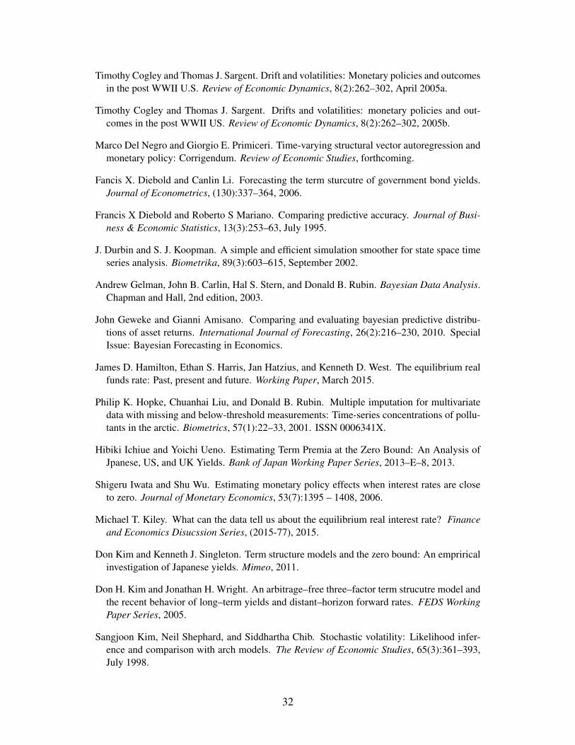
3.1 The Shadow Rate

Our model delivers estimates of the shadow rate of interest that are, by construction, less than

the ELB during the period in which the bound is binding. Panel (a) of Figure 2 shows our

posterior estimates of the shadow rate, along with uncertainty bands. Our model estimates

indicate that the shadow rate fell sharply in early 2009, and began moving up toward the ELB

in early 2013. The last observation in our sample, 2015:Q4, coincides with the last quarter

before short–term interest rate data in the U.S. has begun to rise again above the ELB in recent

years. Indeed, our end-of-sample estimate puts the shadow rate for 2015:Q4 just below the

ELB.


Panel (b) of Figure 2 shows the posterior estimate of the shadow rate when we treat the

interest rate data as missing over the period in which the ELB binds. Interestingly, the ELB

does not pose much of a binding constraint for our sampling technique from 2009-2013, be-

cause the model would have predicted shadow rates below the ELB, even without knowledge

that the ELB was binding in the data. Starting in 2013, there is non-negligible mass above the

ELB when we treat the data as missing, meaning that the information content in the fact that

the ELB was binding is greatest in this part of the ELB sample. Notably, even at the end of our

sample, the ELB is well within the uncertainty bands our model produces for the shadow rate

when we treat the interest rate data as missing.

For comparison, Figure 3 shows the posterior mean of our shadow rate, along with uncer-

tainty bands, on the same plot as estimates from Wu and Xia (2016), and Krippner (2013).10

Two features are worth noting. First, our estimated shadow rate, which also conditions on the

unemployment gap and inflation as business cycle indicators, is lowest during 2009, near the

trough of the Great Recession, according to the NBER. By contrast, the other estimates reach

low points much later. Second, all three estimates are remarkably similar at the end of 2015,

just before the Federal Reserve’s departure from the ELB, even though our model has access

10Measures of the shadow rate from Priebsch (2013) and Ichiue and Ueno (2013) are not shown because theirsample ends in 2013. Their measures are qualitatively similar in that they reach low points well after the trough of therecent recession.

12

to many fewer yields, we do not impose the rigid cross–equation restrictions associated with

no–arbitrage assumptions in the dynamic term–structure literature, and our data sample does

not include the period of departure from the ELB.


3.2 The Real Rate in the Long Run

Figure 4 displays the posterior median of our estimates of the trend real rate, rt, along with

uncertainty bands. Panel (a) of Figure 4 shows quasi real–time estimates of rt, which are con-

ditioned solely on data through period t. Panel (b) of Figure 4 shows the smoothed estimates,

in that the entire data sample is used to estimate the parameters and rt. Notably, the uncertainty

bands surrounding our estimates of rt are wide. This result is consistent with results reported

by Hamilton et al. (2015), Kiley (2015), and Lubik and Matthes (2015).


For both the pseudo–real–time and the smoothed estimates, any estimated downward trend

in the real rate started well before the onset of the Great Recession. Studies like Laubach and

Williams (2015) and Lubik and Matthes (2015) also document downward trajectories in the

trend real rate; however, our estimates do not dip nearly as much as their estimates. One reason

for the differences is our inclusion of stochastic volatility, which allows for large movements in

the gap components of our model in 2008 and 2009. Another is that our estimation procedure

explicitly models the ELB. If we instead ignore the ELB and treat the interest rate data as

observations, we estimate a lower trend nominal interest rate, shown in Figure 5. When the

ELB is ignored, the model is unable to generate a large cyclical movement in interest rates

because it sees the interest rate stop falling at the ELB. As a result the model has difficulty

explaining the prolonged period at the ELB without changes in the trend nominal rate. One

margin by which the trend nominal rate can change is the trend real rate. By contrast, our

model is able to produce a large shadow–rate gap in 2009, which helps explain why observed

nominal interest rates remained at the ELB.


13

3.3 The Effect of Including the Medium–Term Yield

The posterior distribution of the shadow–rate at the ELB is particularly informed by the inclu-

sion of the medium–term yield in our model. When we estimate the model without a medium–

term yield, our posterior distribution of the shadow rate, shown in Panel (a) of Figure 6, is

markedly more dispersed and lower on the eve of the Federal Reserve’s departure from the

ELB in 2015:Q4. The difference from our baseline model, which includes the medium–term

yield, is particularly striking when we consider estimates that treat short–term rates as miss-

ing data during the ELB period, shown in Panel (b) of Figure 6, which is analogous to our

discussion of Figure 2 above.

When shadow–rate estimates for the ELB period are solely informed by data on inflation

and the unemployment–rate gap (and interest rate data up to 2008), the model would have

expected the ELB to bind only for a couple of years, starting to place substantial odds on

positive shadow rates around 2011. In contrast, when the medium–term yield is included

in the estimation, the model predicts negative shadow rate at least until 2014, when short–

term rate data is treated as missing as of 2009. Inclusion of the medium–term yield in our

baseline model thus makes the ELB much less binding for our sampling routine than in the

model without. Insofar as medium-term yields embed information about expected future short

rates, it makes sense that including a medium–term yield will greatly inform our shadow rate

estimates. In the next section we show that our model with the medium–term yield forecasts

short–term interest rates largely better than the model without.


As shown in Panel (c) of Figure 6, the estimated trend real rate is fairly similar to our

baseline estimates when the medium–term yield is excluded from the data. However, the

estimated level of trend inflation is quite different, as shown in panel (d) of the figure. At

the end of our sample, trend inflation derived from the model without the medium-term yield

is markedly lower; which together with the mostly similar trend real rate implies a lower

nominal short–term rate trend estimate in line with the model’s lower estimate of the shadow

rate trajectory shown in Panel (a). Overall, in the model without the medium–term yield, trend

14

inflation is more variable and more closely aligned with 4-quarter changes in the PCE headline

deflator than in the baseline model as the presence of the medium-term yield helps the model

to rationalize a more persistent inflation gap process.

4 Forecasting Interest Rates

Our shadow–rate approach has significant implications for forecasting interest rates. In this

section we offer a number of ways to evaluate our shadow–rate approach by analyzing the

model’s out–of–sample predictions.

4.1 Predictive Density at Selected Dates

To create out–of–sample forecasts from our model, at each date we use the predictive densities

from the posterior distribution (using data only up to that date) to forecast future interest rates.

Our forecasting procedure thus captures uncertainty about both the parameter values and the

unobserved states in our model; details are described in Appendix C. We compare these fore-

casts to the forecasts from the model when we ignore the ELB and feed the interest rate data

into the model without accounting for the ELB.


The left panels of Figure 7 display statistics from the posterior predictive density of the

short–term nominal interest rate from our baseline model at different dates. The forecast hori-

zon extends for five years, and, in addition to mean and median predictions, shaded areas

indicate 50 and 90 percent uncertainty bands. The dashed lines that extend below the ELB

indicate posterior quantiles of the shadow rate distribution (as opposed to the interest rate dis-

tribution). The predictive density of the interest rate is a truncated version of the predictive

density of the shadow rate distribution, so the quantiles of the shadow rate distribution become

exactly the quantiles of the interest rate distribution if the value is larger than the ELB. The

truncation of the shadow–rate distribution causes substantial asymmetry in the interest rate

15

distribution leading to marked differences in the predictive means and medians of our baseline

model.

The right panels of Figure 7 display statistics from the posterior predictive density of the

short–term nominal interest rate when we ignore the ELB. Here, the predicted interest rate

distribution can have negative support because the ELB is ignored. Because the posterior

distribution of the shadow rate is roughly symmetric in our model, the posterior predictive

mean and median do not differ when we ignore the ELB.

In 2008:Q4, the first period before the ELB (Panels (a) and (b) of Figure 7), the model that

ignores the ELB delivers the same forecasts for the shadow rates as our baseline model because

there have been no ELB periods in the estimation and all interest rate data in the sample have

been positive. When the ELB is ignored, shadow–rate forecasts are interest rate forecasts, and

the model predicts future negative rates due to the substantial decline in real activity. Our

baseline model takes the ELB into account and truncates the distribution of expected future

shadow rates to produce interest rate forecasts. In doing so, the mean interest–rate forecast

rises appreciably above the median for several periods.

In 2009:Q1, the period the ELB begins to bind (Panels (c) and (d) of Figure 7), the model

that ignores the ELB produces a different predictive density for the shadow rate than our base-

line model. The reason is that we allow lagged shadow rates to dynamically affect the current

shadow rate. When we ignore the ELB, the lagged shadow rate is the lagged interest rate,

which is higher in this period than our estimated shadow rate because of the ELB. This shifts

up the distribution of expected shadow rates relative to our baseline model, producing notably

more probability of positive interest rates in the subsequent few quarters even as the model

predicts negative interest rates. As shown in Panel (c), accounting for the ELB produces inter-

est rate forecasts that place substantial probability on remaining exactly at the ELB for several

quarters. As in Panel (a), the truncation of the shadow rate distribution in order to produce

interest rate forecasts creates a divergence of mean and median estimates of interest rates for

several years.


16

In 2010:Q4, after the ELB had been binding for some time (panel (a) of figure 8), our

baseline model still predicts substantial probability of interest rates at the ELB because of the

estimated negative shadow rate. Moreover, the median interest rate forecast remains at the

ELB for a number of quarters. By contrast, when the ELB is ignored (panel (b) of figure

8), the model predicts imminent departure from the effective lower bound because it does

not estimate negative shadow rates and instead includes lagged observed interest rates in the

dynamic system, which by construction are higher than our baseline model’s estimated shadow

rates. This difference persists throughout the ELB episode, leading to an extended period in

which ignoring the ELB in the estimation of our model would lead one to predict immediate

departure from the ELB. Toward the end of our sample (2015:Q4, shown in panels (c) and (d)

of Figure 8), the forecasts from the two models are similar, in large part because our estimated

shadow rate is only slightly less than the ELB at that point.

4.2 Forecasting Performance

We utilize the posterior predictive densities to calculate summary statistics in order to assess

the forecasting performance of our baseline model at its variants. We focus on three statistics:

the root–mean–squared error, evaluated at the posterior predictive density’s mean; the mean

absolution deviation, evaluated at the posterior predictive density’s median; and the predictive

score of the posterior distribution (Geweke and Amisano, 2010). We use the mean forecast for

the root–mean–squared error statistic because the mean forecast minimizes expected square

loss, and we use the median forecast for the mean absolute deviation statistic because the

median minimizes expected absolute loss. In addition to our baseline model, we consider the

version of the model where the ELB is ignored and a version of the model that includes the

ELB in the estimation but does not include the medium–term yield.11

Tables 1 and 2 display forecast evaluation statistics for each model variant during our

sample period to 2007 (prior to the ELB) and post 2007 for forecasts of future short–term

interest rates, as well as future medium–term yields. The statistics for our baseline model are

11In the version of the model that ignores the ELB, lagged interest rate data are treated as lagged shadow rates andinterest rate forecasts do not account for the ELB, as in the right–hand panels of Figures 7 and 8.

17

shown as calculated. The statistics for the alternative model specifications are shown on a

relative basis to the baseline model.

[Table 1 about here.]

A key message from Table 1 is that the inclusion of the medium–term yield appears to

help for forecasting short–term interest rates before 2007. At the one–quarter horizon, we

find statistically significant declines in forecast performance for all three of our statistics when

exclude the medium–term yield from our model. Because there are no periods at the ELB

prior to 2007, the root–mean–squared error and mean absolute deviation statistics are identical

for the baseline model and the model where the ELB is ignored for predictions about both

short–term rates and medium–term yields. However, the predictive score statistic indicates

that ignoring the ELB hurts forecasting performance. The reason is that the predictive score

statistic incorporates information about the entire posterior density. During periods in which

the nominal interest rate was low (for example, in 2003), accounting for the ELB has non–

negligible effects on the shape of the predictive density. The predictive score statistic accounts

for this affect, and the results illustrate the benefits of accounting for the ELB for density

forecasts even when the ELB does not yet bind for the observed data.

[Table 2 about here.]

During the sample that includes the ELB, our baseline model almost uniformly out per-

forms the model that ignores the ELB when predicting future short–term interest rates, as

indicated in Panel A of Table 2.12 The baseline model does particularly well when evaluating

forecasts based on the posterior median because this is often exactly at the ELB over the sam-

ple. At the 8–quarter horizon, ignoring the ELB appears to perform somewhat better for the

root–mean–squared error statistic, though not in terms of average absolute deviation from the

predictive median. This finding highlights the implications of using different forecast statistics

in samples affected by the ELB. In particular, the use of mean or median forecasts should be

12Point forecasts from the alternative model that ignores the ELB turn out to be negative during the early stages ofthe ELB period in 2009. Even when these forecasts are set equal to the ELB, they are outperformed by our baselinemodel at similar significance levels both in terms of RMSE and MAD.

18

carefully chosen for the relevant application in a model like ours. For forecasting short–term

interest rates, during the sample that starts after 2007, our baseline model performs similarly to

the model without the medium–term yield. The reason is that both models predict substantial

probability of remaining at the ELB because each model produces estimates of the shadow rate

that are less than zero.

Panel B of Table 2 displays our forecast evaluation statistics for forecasts of the medium–

term yield during the sample that starts in 2008. For each statistic, our baseline model performs

statistically better than the version that ignores the ELB for one–quarter ahead forecasts. The

predictive score statistic also shows that accounting for the ELB improves forecasting perfor-

mance over each of the next four quarters. Thus, our estimates indicate that information about

short–term rates and medium–term yields jointly improve the forecasts of the other, mean-

ing that the statistical connection is non–negligible and that accounting for the ELB improves

density forecasts.


4.3 Forecast Uncertainty

Naturally, the ELB has important effects on the predictive density for nominal interest rates

when the predictive density for shadow rates has non-negligible coverage below the ELB. To

illustrate the relevance of these effects, Figure 9 compares forecast uncertainty in our baseline

model against the alternative when the ELB is ignored. For the purpose of this figure, we

measure forecast uncertainty by the conditional standard deviation of the predictive densities

described above for the nominal short–term rate one and eight-quarters ahead. Overall, near–

and medium–term uncertainty about future short–term rates has mostly declined since the mid-

1980s. Nevertheless, as the level of nominal rates has been trending down over this period as

well, the probability of reaching the ELB has become more and more non-negligible; this is

particularly true for longer–horizons forecasts made since 2000, causing forecast uncertainty

in the baseline model to differ from computations when the ELB is ignored.

Not surprisingly, the onset of the last NBER recession in 2007 is reflected in higher esti-

19

mated levels of stochastic volatility to all shocks in our model, leading to increased shadow–

rate uncertainty. When the ELB is ignored, this directly translates into larger near–term un-

certainty about the nominal short–term interest rate. By accounting for the ELB, our baseline

model recognizes that during the last recession, increased shadow–rate uncertainty is accom-

panied by a marked downward shift of the shadow–rate distribution to values below the ELB

such that the truncated distribution of actual nominal rates almost collapses at values at or

slightly above the ELB. Consequently, near–term uncertainty for short–term nominal rates de-

clines during the last recession when properly accounting for the ELB, as shown in Panel (a)

of Figure 9. In contrast, as shown in Panel (b) of the figure, medium–term uncertainty about

nominal interest rates increases with the increasing shadow–rate uncertainty, though not by

quite as much, as nominal rates are projected to return to their estimated non–negative trend

level.

5 Expected Interest Rate Paths

Our model’s predicted paths for future short–term interest rates imply estimates of expected

interest rate paths, and thus term–premiums for yields along the term–structure of interest

rates. We define the expectations component of a yield on a bond with maturity h periods in

the future as

et,t+h ≡ Et

1

h

h−1∑j=0

it+j

.

The observed longer-term interest rate is given by

et,t+h + pt,t+h

where pt,t+h represents premiums. Note that for any j, Et(it+j) ≥ ELB and the posterior

expectation can be constructed through simulation of the predictive density for nominal short–

term interest rates as described in Appendix C.

20


We focus on the expectations component of the 5–year Treasury yield (yt), which is in

our data set. We construct the expectations component of yt using the out–of–sample posterior

predictive densities at time t. Figure 10 displays our estimated 5–year expectations component,

along with uncertainty bands. Also shown are the expectations component from Kim and

Wright (2005) as well as the 5–year Treasury yield in our data sample.

Despite not imposing the no–arbitrage cross–equation restrictions used in Kim and Wright

(2005), our model produces similar estimates of the expectations component of the 5–year

yield over the sample. The largest deviations are in the early 1990s and during the period in

which the ELB binds. One advantage of our approach to modeling interest rates is that we can

easily incorporate non–stationarity into the inflation process. Given that our estimated trend

inflation rate has fallen since 1990, this may help explain why our estimates of the expectation

component of the 5–year yield are higher than the estimates of Kim and Wright (2005), who

assume that inflation is a stationary process. Interestingly, our model produces larger premiums

than the model of Kim and Wright (2005) during the period in which the ELB binds. While

the truncation of future shadow rates could have produced a higher expectations component

for our model, it appears that the lagged shadow rates keep the interest rate low enough for

long enough to produce relatively low paths for interest rates.

Notably, the uncertainty bands in Figure 10 are not of constant width. The stochastic

volatility in our model leads to changes in the width of uncertainty bands, which is especially

pronounced at the beginning of the Great Recession, a period in which our model estimates

that volatility rose appreciably.

6 Conclusion

In this paper, we develop a methodology to account for the ELB in otherwise

conditionally–linear Gaussian time series models. Further, we demonstrate how to estimate

the parameters and latent states of such a model with an otherwise standard Bayesian MCMC

sampler.

21

We document that including the ELB can have drastic effects for interest rate forecasts,

as well as the expectations component of longer–term yields and thus also the computation

of term–premiums. Further, accounting for the ELB using our shadow–rate approach appears

to improve forecast performance. We also estimate changes in the trend real rate, defined as

a long–term forecast of the real interest rate, and find that any decline in the trend real rate

since the onset of the Great Recession is best characterized as a continuation of a downward

trajectory that began well before.

APPENDIX

A Sampling States with Censored Data

Our Gibbs sampling procedure is a generalization of Park et al. (2007) that applies the method-

ology of Hopke et al. (2001). Assume that the vector ξt is a random variable that evolves so

that

ξt = Atξt−1 + Btεt (13)

where εt is a vector of standard normal random variables of appropriate length and the se-

quence of matrices AtTt=1 and BtTt=1 are given.13

Define the vector

Xt = Ctξt (14)

where the sequence of matrices CtTt=1 are known.14 We assume that Xt has a partition

made up of a vector shadow rates, (St), and a partition of variables that are unconstrained by

13In our application, described in the main body of the paper note that we have a constant At = A.14In our application, described in the main body of the paper note that we have a constant Ct = C.

22

the ELB, (M t).15 That is,

Xt =

StM t

(15)

The observed data are

Zt =

max (St, ELB)

M t

(16)

where the max operator is applied element by element. The ELB acts as a censoring function

in the model through the max operator, though more general censoring functions could be

used.

DefineX ≡ [X ′1,X′2, . . . ,X

′T ]′, and Z ≡ [Z ′1,Z

′2, . . . ,Z

′T ]′. We split Z into two parts,

one part containing all non-interest rate data and all observations for interest rates that are not

constrained by the ELB, ZNC , and another part with the interest rate data constrained at the

ELB, ZC .16 The corresponding elements of X are XNC and XC . Note that, the elements of

XC are all shadow rates that are less than the ELB.

Given a normal distribution for ξ0, it follows that the vectorsXNC and ξ = [ξ′1, ξ′2, . . . , ξ

′T ]′

have a multivariate normal (prior) distribution

XNC

ξ

∼ NµXµξ

,V XX V X,ξ

V ξ,X V ξ,ξ

(17)

and we can derive the posterior distribution for ξ conditional on observed interest rates, when

the ELB is not binding, as well as all observations for macroeconomic, non-interest-rate vari-

ables (M t):

ξ∣∣ (XNC = ZNC

)∼ N

(µξ, V ξ,ξ

). (18)

15In the application described above, there are in principle two shadow rates, one associated with the short–terminterest rate and one associated with the medium–term yield described; in practice, the ELB constraint has beenbinding only for the former, however.

16Accordingly, ZC consists solely of observations for interest rates that are equal to ELB.

23

In general, the posterior moments in (18) are given by

µξ = µξ +K(ZNC − µX

)with K = V ξ,XV

−1XX (19)

and V ξ,ξ = V ξ,ξ − V ξ,XV−1XXV X,ξ . (20)

Typically, these posterior moment matrices will by quite large; µξ is, for example, a vector

of length T × Nξ = 224 × 12 = 2, 688 in our application, However, the Kalman smoother,

adapted for handling missing observations for interest rates when the ELB binds, provides a

convenient way to recursively compute the moments in (19) and (20) while recovering the

distribution of ξ conditional on observations for ZNC . To this point, our procedure amounts

to treating the observations for ZC as missing data.17

We then note that the information contained in the interest rate data at the ELB is that

XC ≤ ELB (for every element of XC). The posterior distribution of ξ, conditional on Z, is

then

ξ|(X = Z) ∼ TN(µξ, V ξ,ξ;X

C ≤ ELB)

(21)

where TN stands for a truncated normal such that its density function is

Pr (ξ|Z) ∝ φ(µξ, V ξ,ξ

)1(XC ≤ ELB) (22)

where φ is the multivariate normal density function andXC is a shadow rate draw where every

element is below the ELB. To sample from the posterior distribution of ξ conditional on all

observations in Z, we first draw ξ from Pr(ξ∣∣XNC = ZNC

). We then reject draws until

we find a draw that satisfies the requirement that XC ≤ ELB for every element. Rejection

sampling is thus done on an entire draw of ξ, which corresponds to an entire draw of the time

series for ξt.

In our baseline framework, lagged values of ξt appear as explanatory variables and are not

17Alternatively, Chan and Jeliazkov (2009) describe ways to efficiently compute the moments in (19) and (20) basedon sparse matrices that exploit the state space structure inherent in (17).

24

censored. A straightforward extension is to incorporate a given number of p lags of Zt, which

includes interest rate data that can be constrained the ELB. In this case, we change (13) to be

ξt = Atξt−1 + F tζt−1 + Btεt (23)

ζt−1 ≡ [Z ′t−1,Z′t−2, . . . ,Z

′t−p]

′ (24)

where F tTt=1 are conformable matrices that are known. The posterior of ξ can be constructed

exactly as in our baseline model, treating ζt−1Tt=1 as exogenous in every period because the

rejection step will ensure that the sampled values of ξ are consistent with ζt−1 for all t. For

comparison, the models of Iwata and Wu (2006) and Nakajima (2011) can be cast, conditional

on parameter values, as special cases of this setup in which the matrix At = 0. A notable

difference in the posterior simulation of the model is that the truncated distributions in Iwata

and Wu (2006) and Nakajima (2011) can be cast as period–by–period truncated normals. By

contrast, our posterior estimates require rejection sampling on an entire time series draw of ξ.

B Priors and Posterior Sampling

MCMC estimates of the model are obtained from a Gibbs sampler. The sampler is run multiple

times with different starting values and convergence is assessed with the scale reduction test

of Gelman et al. (2003).18 For each run, 20, 000 draws are stored after a burn-in period of

100, 000 draws; the post-burnin draws from each run are then merged.

Our models consist of two vectors of latent states:

ξt =

[πt rt st yt πt ut st yt eπ,t

]′

and ht =

[log (σ2

π,t) log (σ2π,t) log (σ2

u,t) log (σ2s,t) log (σ2

y,t) log (σ2e,t)

]′18Specifically, for every model, 10 independent runs for the Gibbs sampler were evaluated; each run initialized

with different starting values drawn from the model’s prior distribution. Convergence is deemed satisfactory whenthe scale reduction statistics for every parameter and latent variable are below 1.2; (values close to 1 indicate goodconvergence).

25

as well as the parameters governing the means and volatility of shocks to ht, see (7), stacked in

the vectors µ and φ2,19 the variance of shocks to the trend real rate, denoted σ2r , the transition

coefficients of the gap VAR (6), stacked in a vector a, and lower diagonal elements of gap

shock loadings B in (6) that can be stacked in a vector denoted b. For ease of reference,

all parameters are collected in the vector θ =

[a′ b′ σ2

r φ2′, µ′]′

. Furthermore, since

MCMC estimates of hT will be obtained from the multi–move filter of Kim et al. (1998), the

use of a set of discrete indicator variables, sT , is required to to approximate log η2j,t in (7) with

a mixture of normals. Conditional on draws for the parameters, (θ), and log-volatilities hT ,

we can construct matrices A, BtTt=1, and C and to obtain the linear, Gaussian state space

system described by equations (13) and (14) in Appendix A.

For the initial values of the latent states, the following priors were used:

ξ0 ∼ N (E(ξ0),Ω) with E(ξ0) =

ξ0

and Ω =

Ω 0

0 Ω

(25)

An uninformative prior for the initial gap levels is obtained by setting Ω equal to the ergodic

variance-covariance matrix of the gaps implied by the VAR (6), evaluated at the time zero

draws for the stochastic volatilities, encoded in Σ0, for every MCMC draw.20 The prior for the

initial trend levels are set to be consistent with

π0

s0

y0

∼ N

2

4

5

,

16 −16 −16

−16 116 16

−16 16 116

(26)

which implies a fairly vague prior level of the real-rate trend, rt = st − πt while taking

correlated signals about the initial level of trend inflation from readings on all three nominal

variables.19The auto-regressive coefficients ρj in each of the stochastic volatility equations in (7) are fixed at 0.99.20In the case of a VAR(1), the ergodic variance-covariance matrix solves Ω = AΩA′ +BΣ0B

′ for given valuesofA,B, and Σ0.

26

The prior for the average level of the log-variances is:

µj ∼ N(

2 · log1

10− 25

2, 25

)⇒ E(σt) =

1

10(27)

The prior distribution for each of the the parameters for the parameters φ2 is a univariate

inverse–Wishart distribution with 30 degrees of freedom (corresponding to an inverse gamma

with a shape parameter set equal to a value of 15) and a mean equal to 0.22 which coincides

with the fixed coefficient-value of 0.2 used by Stock and Watson (2007) in their univariate

model for inflation.

The parameter governing the variability of real-rate trend shocks, σ2r , has a univariate

inverse–Wishart distribution with 3 degrees of freedom (corresponding to an inverse–gamma

distribution with a shape parameter equal to 1.5 degrees of freedom) and is centered around

a prior mean of 0.22. While this vaguely informative prior embeds the belief that the trend

shocks explain only a small share of variations in real rates, it also helps to avoid the pile–up

problem — known, for example, from Stock and Watson (1998) and considered in the context

of estimating σ2r also by Laubach and Williams (2003) as well as Clark and Kozicki (2005) —

by keeping posterior draws for the parameter away from zero.

While the priors for a and b are taken to be completely diffuse, starting values for the

Gibbs sampler are drawn from the following normal distributions:

a ∼ N(0, 0.32 · I

)b ∼ N (0, I) (28)

The Gibbs sampler is initialized with values drawn from the prior for hT and θ and then

generates draws from the joint posterior distribution

p(ξT ,hT ,a, b, σ2

r ,µ,φ2, sT

∣∣Y T)

by iterating over draws from the following conditional distributions:

1. Draw from p(ξT∣∣hT ,a, b, σ2

r ,φ2,µ, Y T

)with the disturbance smoothing sampler of

Durbin and Koopman (2002) and rejection sampling for the shadow rate when the ob-

27

served nominal short–term rate is at the ELB as described in Appendix A.

2. Draw from p(a∣∣ξT ,hT , b, σ2

r ,φ2,µ, Y T

)= p

(a∣∣ξT ,hT , b), a normal conjugate pos-

terior for a VAR with known heteroscedasticity, with rejection sampling to ensure a

stationary VAR (Cogley and Sargent, 2005a; Clark, 2011)

3. Draw from p(b∣∣ξT ,hT ,a, σ2

r ,φ2,µ, Y T

)via recursive Bayesian regressions with

known heteroscedasticity to orthogonalize the gap shocks of the VAR in (6).

4. Draw from the inverse-gamma conjugate posteriors for σ2r :

p(σ2r

∣∣ξT ,hT ,a, b,φ2,µ, Y T)

= p(σ2r

∣∣ξT )

5. Draw from the inverse-gamma conjugate posteriors for φ2:

p(φ2∣∣ξT ,hT ,a, b, σ2

r ,µ, YT)

= p(φ2∣∣hT )

6. Draw the mixture indicators sT from:

p(sT∣∣ξT ,hT ,a, b, σ2

r ,φ2,µ, Y T

)

7. Draw from p(hT ,µ

∣∣sT , ξT ,a, b, σ2r ,φ

2, Y T)

= p(hT∣∣sT , ξT , φ2

)embedding the dis-

turbance smoothing sampler of Durbin and Koopman (2002) in a linear state space for(hT ,µ

)as in Kim et al. (1998).21

Strictly speaking, this is not a simple Gibbs sampler consisting of steps 1 – 7, but rather a

Gibbs-within-Gibbs sampler with the outer Gibbs sampler iterating between

p(sT , ξT ,θ

∣∣hT , Y T)

(thus, a block consisting of steps 1 through 6)

and p(hT ,µ

∣∣sT , ξT ,a, b, σ2r ,φ

2, Y T)

(step 7),

similar to the discussion by Del Negro and Primiceri (forthcoming).

21The constant µ is embedded in the state space as a unit root without shocks, which improves the efficiency of theGibbs sampler by jointly sampling hT and µ.

28

C Computation of Predictive Densities

In order to derive predictive densities for interest rates (and other data in Zt), we first proceed

by characterizing the predictive density for the shadow rate, included in the non-censored

vector of variables Xt described in Appendix A. Apart from handling the truncation issues

related to the ELB, our approach is fairly standard, building, for example, on the work by

Geweke and Amisano (2010), Christoffel et al. (2010), and Warne et al. (2015). Given the

truncation issues for interest rates and the fat tails introduced into the predictive density by

the stochastic volatility specification, we have chosen to compute the predictive density based

on the mixture of normals that is implied by the draws from our MCMC sampler, instead

of approximating the predictive density solely based on its first two moments, treating the

predictive density as a normal distribution, as has been done, for example, by Adolfson et al.

(2007) in the case of linearized, constant-parameter DSGE models.

In order to compute the predictive density for Zt+h jumping off data at time t, we first

employ the MCMC sampler described in Appendix B to re-estimate all model parameters and

latent variables (θ, ξ1:t and h1:t) conditional on data available through time t. Draws from this

MCMC sampler will henceforth be indexed by k.

Conditional on draws (ξkt ,hkt ,θ

k), it is straightforward to compute the predictive mean for

uncensored variables:

E(Xt+h

∣∣ξkt ,hkt ,θk) = Ck(Ak)hξkt (29)

and the predictive mean, conditional solely on data through t, can then be approximated by

averaging over the means derived from each MCMC draw:

E (Xt+h|Z1:t) ≈∑k

E(Xt+h

∣∣ξkt ,hkt ,θk) (30)

However, in order to characterize the entire predictive density for uncensored variables or

even the predictive density for interest rates, which are subject to censoring due to the ELB

constraint, we need to account for non-linearities in the distribution for future ξt:t+h arising

29

from the stochastic volatility shocks in our model. To do so, we simulate J = 100 trajecto-

ries, each indexed by j, of hk,jt:t+h for each draw k from the MCMC sampler. Conditional on

(ξkt ,hkt ,θ

k) as well as hk,jt:t+h, ξt:t+h and Xt:t+h are normally distributed. The means of the

conditional normals are still given by (29), and the variances are given by

Var(ξt+h

∣∣ξkt ,hkt ,hk,jt+1:t+h,θk)

=h∑i=0

(Ak)i

Σt+ik,j

((Ak)i)′

(31)

Var(Xt+h

∣∣ξkt ,hkt ,hk,jt+1:t+h,θk)

= Ck Var(ξt+h

∣∣ξkt ,hkt ,hk,jt+1:t+h,θk)(

Ck)′

(32)

Recall that Xt:t+h contains shadow rates St:t+h and the predictive density for nominal

interest rates can be constructed by computing the moments and density function of the trun-

cated normal distribution conditional on every pair of draws (k, j). Specifically, consider the

short–term shadow rate st+h and denote its conditional predictive mean and variance for draw

(k, j), computed according to (29) and (32), by mk,j = mk and vk,j . The predictive density

for it = max (st, ELB), conditional on draw (k, j), is then characterized by:

P k,j ≡ Pr(st+h < ELB|·) (33)

pk,j ≡ φ(st+h < ELB|·) (34)

E (it+h|·) = P k,j · ELB + (1− P k,j) ·(mk,j +

√vk,j

pk,j

P k,j

)(35)

Var (it+h|·) = (1− P k,j) · vk,j(

1 +(ELB −mk,j)pk,j√

vk,jP k,j+

(pk,j

P k,j

)2)

(36)

f (it+h|·) = 1(it+h = ELB)P k,j . . .+ (37)

+ 1(it+h > ELB)(1− P k,j) ·φ(

(it+h −mk,j)/√vk,j)

√vk,jP k,j

(38)

where “·” in “(it+h|·)” is a placeholder for the conditioning set(ξkt ,h

kt ,h

k,jt+1:t+h,θ

k)

, and

φ(·) is the standard normal pdf .

Based on these conditional distribution for every draw (k, j) we construct predictive means

and variances by aggregating across draws using the law of iterated expectations and the law of

30

total variance, respectively. Predictive medians are obtained from simulated draws of it+h for

every draw (k, j) and computing the 50% quantile across all draws. The time t contribution

to the predictive scores are computed from averaging across draws the conditional likelihoods

f (it+h|·); as in Geweke and Amisano (2010) the predictive score for an evaluation window

ranging from t = T1 through t = T2 is then given as

PS =1

T2 − T1 + 1

T2∑t=T1

log f (it+h|Z0:t) . (39)

ReferencesMalin Adolfson, Jesper Linde, and Mattias Villani. Forecasting Performance of an Open Econ-

omy DSGE Model. Econometric Reviews, 26(2-4):289–328, 2007.

Michael D. Bauer and Glenn D. Rudebusch. Monetary policy expectations at the zero lowerbound. Federal Reserve Bank of San Francisco Working Paper Series, 2014.

Stephen Beveridge and Charles R. Nelson. A new approach to decomposition of economic timeseries into permanent and transitory components with particular attention to measurementof the ’business cycle’. Journal of Monetary Economics, 7(2):151–174, 1981.

Fischer Black. Interest rates as options. The Journal of Finance, 50(5):1371–1376, 1995.

John Y. Campbell and Robert J. Shiller. Cointegration and tests of present value models. TheJournal of Political Economy, 95(5):1062–1088, October 1987.

John Y. Campbell and Robert J. Shiller. Yield spreads and interest rate movements: A bird’seye view. The Review of Economic Studies, 58(3):495–514, 1991.

Joshua C.C. Chan and Ivan Jeliazkov. Efficient simulation and integrated likelihood estimationin state space models. International Journal of Mathematical Modelling and NumericalOptimization, 1(1/2):101–120, 2009.

Joshua C.C. Chan and Rodney Strachan. The zero lower bound: Implications for modellingthe interest rate. Working Paper, 2014.

Kai Christoffel, Anders Warne, and Gnter Coenen. Forecasting with DSGE models. WorkingPaper Series 1185, European Central Bank, May 2010.

Todd E. Clark. Real-time density forecasts from bayesian vector autoregressions with stochas-tic volatility. Journal of Business & Economic Statistics, 29(3):327–341, 2011.

Timothey Cogley and Thomas J. Sargent. Measuring price level uncertainty and instability inthe U.S., 1850–2012. Review of Economics and Statistics, Forthcoming.

31

Timothy Cogley and Thomas J. Sargent. Drift and volatilities: Monetary policies and outcomesin the post WWII U.S. Review of Economic Dynamics, 8(2):262–302, April 2005a.

Timothy Cogley and Thomas J. Sargent. Drifts and volatilities: monetary policies and out-comes in the post WWII US. Review of Economic Dynamics, 8(2):262–302, 2005b.

Marco Del Negro and Giorgio E. Primiceri. Time-varying structural vector autoregression andmonetary policy: Corrigendum. Review of Economic Studies, forthcoming.

Fancis X. Diebold and Canlin Li. Forecasting the term sturcutre of government bond yields.Journal of Econometrics, (130):337–364, 2006.

Francis X Diebold and Roberto S Mariano. Comparing predictive accuracy. Journal of Busi-ness & Economic Statistics, 13(3):253–63, July 1995.

J. Durbin and S. J. Koopman. A simple and efficient simulation smoother for state space timeseries analysis. Biometrika, 89(3):603–615, September 2002.

Andrew Gelman, John B. Carlin, Hal S. Stern, and Donald B. Rubin. Bayesian Data Analysis.Chapman and Hall, 2nd edition, 2003.

John Geweke and Gianni Amisano. Comparing and evaluating bayesian predictive distribu-tions of asset returns. International Journal of Forecasting, 26(2):216–230, 2010. SpecialIssue: Bayesian Forecasting in Economics.

James D. Hamilton, Ethan S. Harris, Jan Hatzius, and Kenneth D. West. The equilibrium realfunds rate: Past, present and future. Working Paper, March 2015.

Philip K. Hopke, Chuanhai Liu, and Donald B. Rubin. Multiple imputation for multivariatedata with missing and below-threshold measurements: Time-series concentrations of pollu-tants in the arctic. Biometrics, 57(1):22–33, 2001. ISSN 0006341X.

Hibiki Ichiue and Yoichi Ueno. Estimating Term Premia at the Zero Bound: An Analysis ofJpanese, US, and UK Yields. Bank of Japan Working Paper Series, 2013–E–8, 2013.

Shigeru Iwata and Shu Wu. Estimating monetary policy effects when interest rates are closeto zero. Journal of Monetary Economics, 53(7):1395 – 1408, 2006.

Michael T. Kiley. What can the data tell us about the equilibrium real interest rate? Financeand Economics Disucssion Series, (2015-77), 2015.

Don Kim and Kenneth J. Singleton. Term structure models and the zero bound: An empriricalinvestigation of Japanese yields. Mimeo, 2011.

Don H. Kim and Jonathan H. Wright. An arbitrage–free three–factor term strucutre model andthe recent behavior of long–term yields and distant–horizon forward rates. FEDS WorkingPaper Series, 2005.

Sangjoon Kim, Neil Shephard, and Siddhartha Chib. Stochastic volatility: Likelihood infer-ence and comparison with arch models. The Review of Economic Studies, 65(3):361–393,July 1998.

32

Robert G. King and Andre Kurmann. Expectations and the term structure of interest rates:Evidence and implications. Federal Reserve Bank of Richmond Economic Quarterly, (Fall):49–95, August 2002.

Todd E. Clark and Sharon Kozicki. Estimating equilibrium real interest rates in real time. TheNorth American Journal of Economics and Finance, 16(3):395–413, December 2005.

Leo Krippner. Measuring the stance of monetary policy in zero lower bound environments.Economics Letters, 118(1):135–138, 2013.

Leo Krippner. Zero Lower Bound Term Structure Modeling: A practitioner’s Guide. PalgraveMacmillan, 2015.

Thomas Laubach and John C. Williams. Measuring the natural rate of interest. The Review ofEconomics and Statistics, 85(4):1063–1070, November 2003.

Thomas A. Laubach and John C. Williams. Measuring the natural rate of interest redux.Hutchins Center on Fiscal & Monetary Policy at Brookings, (15), 2015.

Marco J. Lombardi and Fen Zhu. A shadow policy rate to calibrate US monetary policy at thezero lower bound. BIS Working Paper, 425, 2014.

Thomas A. Lubik and Christian Matthes. Calculating the natural rate of interest: A comparisonof two alternative approaches. Economic Brief, (15-10), 2015.

Elmar Mertens. Measuring the level and uncertainty of trend inflation. Review of Economicsand Statistics, forthcoming.

Jouchi Nakajima. Monetary policy transmission under zero interest rates: An extended time-varying parameter vector autoregression approach. Bank of Japan Working Paper Series,2011.

Jung Wook Park, Marc G. Genton, and Sujit K. Ghosh. Censored time series analysis withautoregressive moving average models. The Canadian Journal of Statistics / La RevueCanadienne de Statistique, 35(1):151–168, 2007.

Marcel A. Priebsch. Computing arbitrage-free yields in multi-factor gaussian shadow-rate termstructure models. Finance and Economics Disucssion Series, (2013-63), 2013.

Giorgio E. Primiceri. Time varying structural vector autoregressions and monetary policy. TheReview of Economic Studies, 72(3):821–852, 2005.

Lukasz Rachel and Thomas D. Smith. Secular drivers of the global real interest rate. Bank ofEngland Staff Working Paper, (571), 2015.

Christopher A. Sims. Macroeconomics and reality. Econometrica, 48(1):1–48, 1980.

James H. Stock and Mark W. Watson. Median unbiased estimation of coefficient variance ina time-varying parameter model. Journal of the American Statistical Association, 93(441):349–358, 1998.

James H. Stock and Mark W. Watson. Why has U.S. inflation become harder to forecast?Journal of Money, Credit and Banking, 39(S1):3–33, February 2007.

33

Lawrence H. Summers. U.S. economic prospects: Secular stagnation, hysteresis and the zerolower bound. Buiness Economics, 49(2):65–73, 2014.

Anders Warne, Gnter Coenen, and Kai Christoffel. Marginalized predictive likelihood com-parisons of linear gaussian state-space models with applications to DSGE, DSGE-VAR, andVAR models. mimeo European Central Bank, December 2015.

Cynthia Wu and Fan Dora Xia. Measuring the macroeconomic impact of monetary policy atthe zero lower bound. Journal of Money, Credit, and Banking, 48(2–3):253–291, 2016.

34

Figure 1: Data and Estimated Trends

1960 1970 1980 1990 2000 20100

2

4

6

8

10

12

14

16

18

(a) Federal Funds Rate

1960 1970 1980 1990 2000 20100

2

4

6

8

10

12

14

16

18

(b) 5–Year Treasury Yield

1960 1970 1980 1990 2000 2010−6

−4

−2

0

2

4

6

8

10

12

(c) PCE Inflation Rate

1960 1970 1980 1990 2000 2010−3

−2

−1

0

1

2

3

4

5

(d) Unemployment–Rate Gap

Note: Red solid lines are data. Shaded areas indicate 50 and 90 percent uncertainty bands, dashedlines are posterior means. The posterior distribution is derived from conditioning the model onthe entire data sample 1960:Q1 – 2015:Q4. Uncertainty bands reflect the joint uncertainty aboutmodel parameters and states. Dotted vertical lines indicate NBER recession peaks and troughs.

35

Figure 2: Shadow Rate Estimates

2007 2008 2009 2010 2011 2012 2013 2014 2015−4

−2

0

2

4

6

(a) Baseline Model

2007 2008 2009 2010 2011 2012 2013 2014 2015−4

−2

0

2

4

6

(b) Treating ELB Data as Missing

Note: Shaded areas indicate 50 and 90 percent uncertainty bands, dashed lines are posteriormeans. The posterior distribution is derived from conditioning the model on the entire data sample1960:Q1 – 2015:Q4. Uncertainty bands reflect the joint uncertainty about model parameters andstates. Results in Panel (b) are conditioned on a data set where observations on short–term ratesare treated as missing data during the ELB period.

36

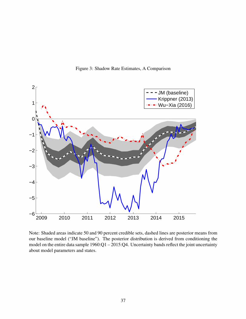
Figure 3: Shadow Rate Estimates, A Comparison

2009 2010 2011 2012 2013 2014 2015−6

−5

−4

−3

−2

−1

0

1

2JM (baseline)Krippner (2013)Wu−Xia (2016)

Note: Shaded areas indicate 50 and 90 percent credible sets, dashed lines are posterior means fromour baseline model (“JM baseline”). The posterior distribution is derived from conditioning themodel on the entire data sample 1960:Q1 – 2015:Q4. Uncertainty bands reflect the joint uncertaintyabout model parameters and states.

37

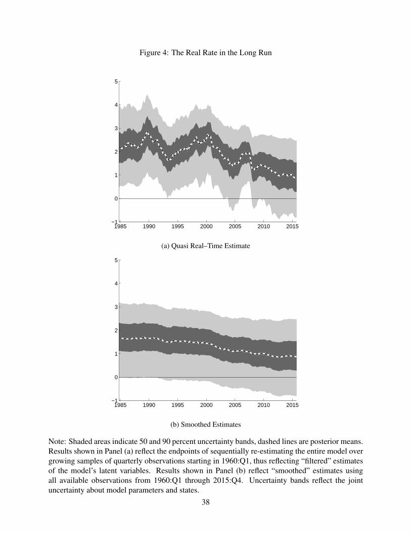
Figure 4: The Real Rate in the Long Run

1985 1990 1995 2000 2005 2010 2015−1

0

1

2

3

4

5

(a) Quasi Real–Time Estimate

1985 1990 1995 2000 2005 2010 2015−1

0

1

2

3

4

5

(b) Smoothed Estimates

Note: Shaded areas indicate 50 and 90 percent uncertainty bands, dashed lines are posterior means.Results shown in Panel (a) reflect the endpoints of sequentially re-estimating the entire model overgrowing samples of quarterly observations starting in 1960:Q1, thus reflecting “filtered” estimatesof the model’s latent variables. Results shown in Panel (b) reflect “smoothed” estimates usingall available observations from 1960:Q1 through 2015:Q4. Uncertainty bands reflect the jointuncertainty about model parameters and states.

38

Figure 5: The Trend Nominal Rate when the ELB is Ignored

2009 2010 2011 2012 2013 2014 20150

1

2

3

4

5BaselineELB ignored

Note: Shaded area indicates 50 percent uncertainty bands and the dashed line is the mean estimatefor our baseline model. This solid red lines indicate 50 percent uncertainty bands and the thicksolid red line is the mean estimate when we ignore the ELB. The posterior distribution is derivedfrom conditioning the model on the entire data sample 1960:Q1 – 2015:Q4. Uncertainty bandsreflect the joint uncertainty about model parameters and states.

39

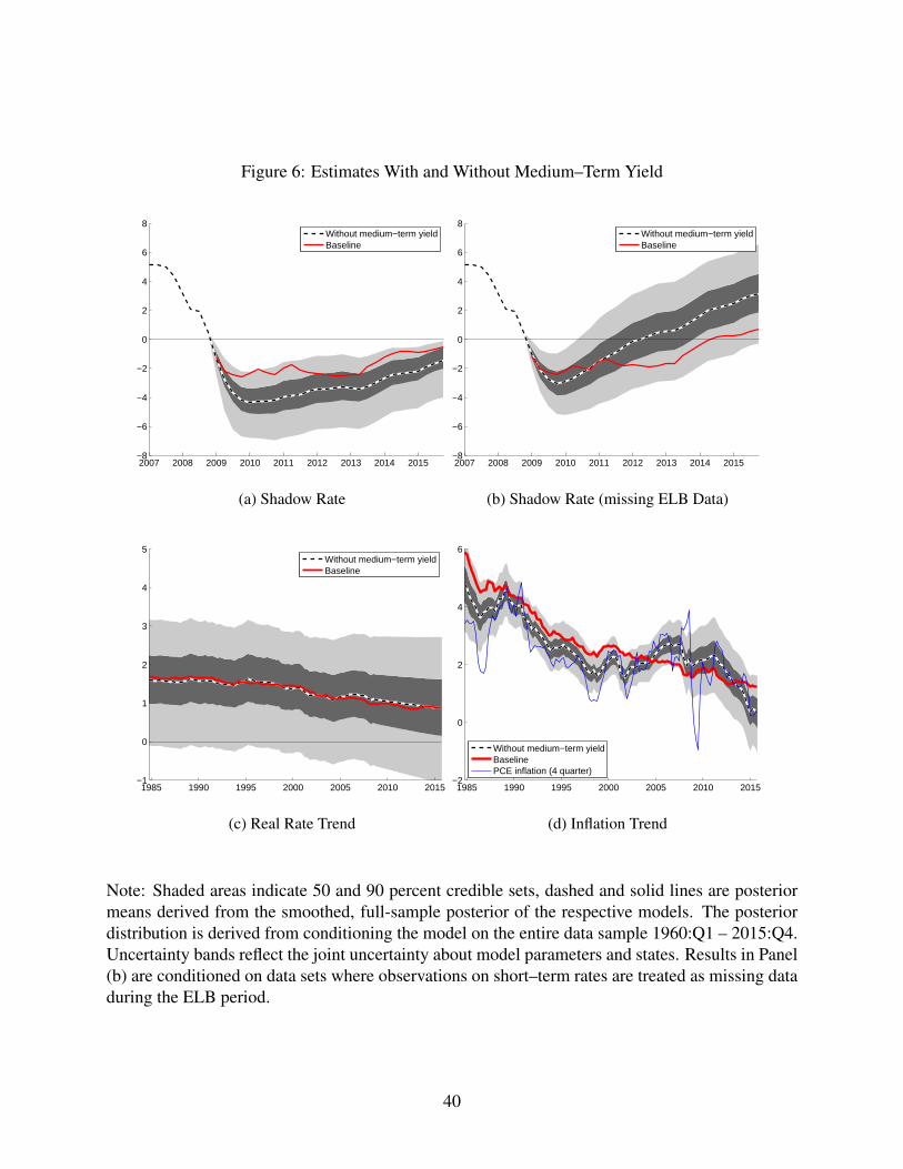
Figure 6: Estimates With and Without Medium–Term Yield

2007 2008 2009 2010 2011 2012 2013 2014 2015−8

−6

−4

−2

0

2

4

6

8Without medium−term yieldBaseline

(a) Shadow Rate

2007 2008 2009 2010 2011 2012 2013 2014 2015−8

−6

−4

−2

0

2

4

6


(b) Shadow Rate (missing ELB Data)

1985 1990 1995 2000 2005 2010 2015−1

0

1

2

3

4


(c) Real Rate Trend

1985 1990 1995 2000 2005 2010 2015−2

0

2

4

6

Without medium−term yieldBaselinePCE inflation (4 quarter)

(d) Inflation Trend

Note: Shaded areas indicate 50 and 90 percent credible sets, dashed and solid lines are posteriormeans derived from the smoothed, full-sample posterior of the respective models. The posteriordistribution is derived from conditioning the model on the entire data sample 1960:Q1 – 2015:Q4.Uncertainty bands reflect the joint uncertainty about model parameters and states. Results in Panel(b) are conditioned on data sets where observations on short–term rates are treated as missing dataduring the ELB period.

40

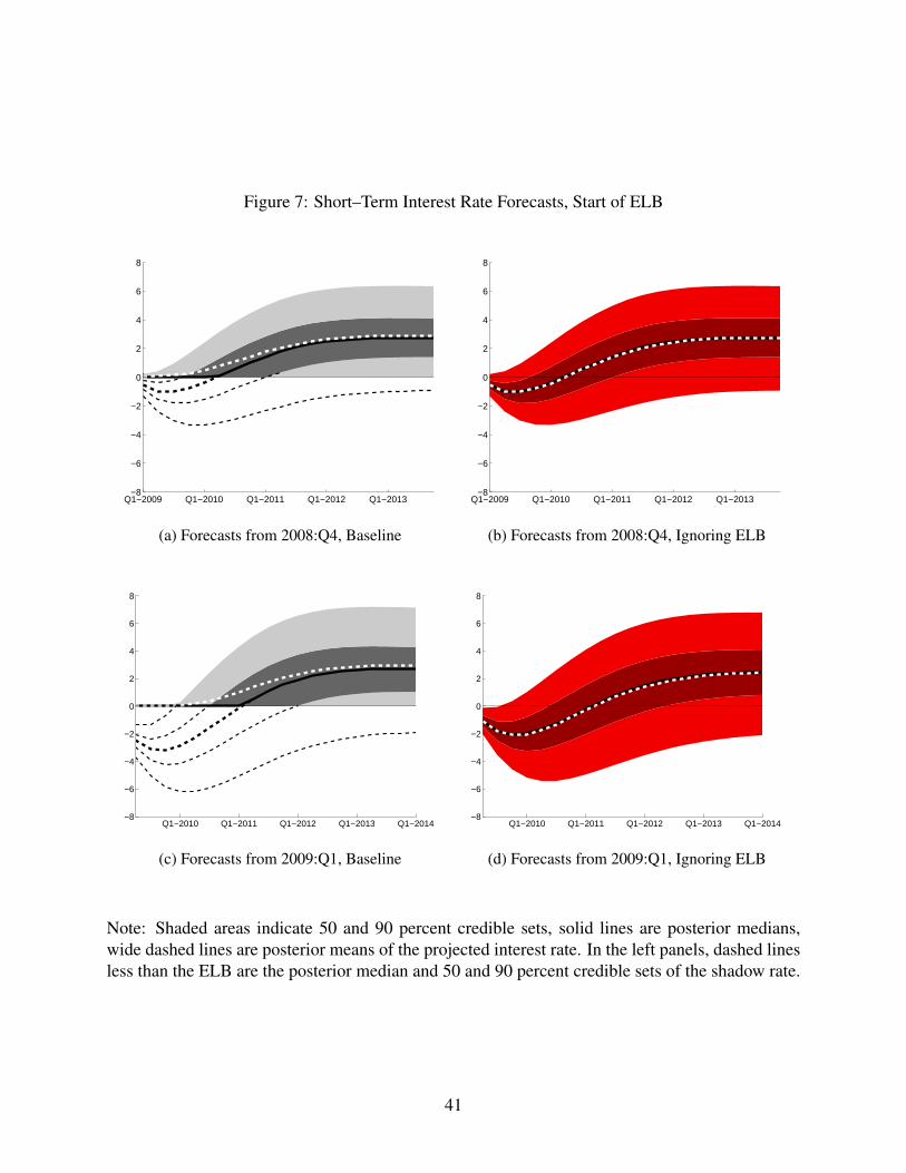
Figure 7: Short–Term Interest Rate Forecasts, Start of ELB

Q1−2009 Q1−2010 Q1−2011 Q1−2012 Q1−2013−8

−6

−4

−2

0

2

4

6

8

(a) Forecasts from 2008:Q4, Baseline

Q1−2009 Q1−2010 Q1−2011 Q1−2012 Q1−2013−8

−6

−4

−2

0

2

4

6

8

(b) Forecasts from 2008:Q4, Ignoring ELB

Q1−2010 Q1−2011 Q1−2012 Q1−2013 Q1−2014−8

−6

−4

−2

0

2

4

6

8

(c) Forecasts from 2009:Q1, Baseline

Q1−2010 Q1−2011 Q1−2012 Q1−2013 Q1−2014−8

−6

−4

−2

0

2

4

6

8

(d) Forecasts from 2009:Q1, Ignoring ELB

Note: Shaded areas indicate 50 and 90 percent credible sets, solid lines are posterior medians,wide dashed lines are posterior means of the projected interest rate. In the left panels, dashed linesless than the ELB are the posterior median and 50 and 90 percent credible sets of the shadow rate.

41

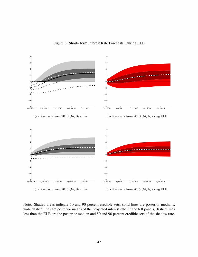
Figure 8: Short–Term Interest Rate Forecasts, During ELB

Q1−2011 Q1−2012 Q1−2013 Q1−2014 Q1−2015−8

−6

−4

−2

0

2

4

6

8

(a) Forecasts from 2010:Q4, Baseline

Q1−2011 Q1−2012 Q1−2013 Q1−2014 Q1−2015−8

−6

−4

−2

0

2

4

6

8

(b) Forecasts from 2010:Q4, Ignoring ELB

Q1−2016 Q1−2017 Q1−2018 Q1−2019 Q1−2020−8

−6

−4

−2

0

2

4

6

8

(c) Forecasts from 2015:Q4, Baseline

Q1−2016 Q1−2017 Q1−2018 Q1−2019 Q1−2020−8

−6

−4

−2

0

2

4

6

8

(d) Forecasts from 2015:Q4, Ignoring ELB

Note: Shaded areas indicate 50 and 90 percent credible sets, solid lines are posterior medians,wide dashed lines are posterior means of the projected interest rate. In the left panels, dashed linesless than the ELB are the posterior median and 50 and 90 percent credible sets of the shadow rate.

42

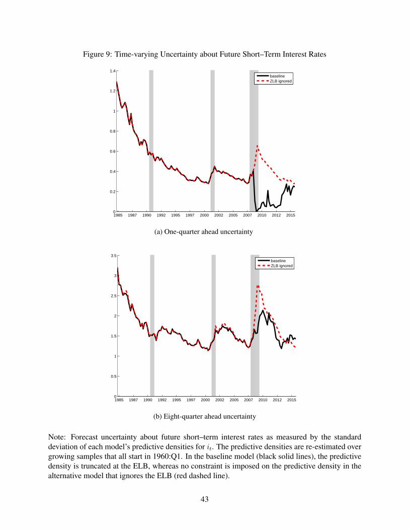
Figure 9: Time-varying Uncertainty about Future Short–Term Interest Rates

1985 1987 1990 1992 1995 1997 2000 2002 2005 2007 2010 2012 20150

0.2

0.4

0.6

0.8

1

1.2

1.4baselineZLB ignored

(a) One-quarter ahead uncertainty

1985 1987 1990 1992 1995 1997 2000 2002 2005 2007 2010 2012 20150

0.5

1

1.5

2

2.5

3

3.5baselineZLB ignored

(b) Eight-quarter ahead uncertainty

Note: Forecast uncertainty about future short–term interest rates as measured by the standarddeviation of each model’s predictive densities for it. The predictive densities are re-estimated overgrowing samples that all start in 1960:Q1. In the baseline model (black solid lines), the predictivedensity is truncated at the ELB, whereas no constraint is imposed on the predictive density in thealternative model that ignores the ELB (red dashed line).

43

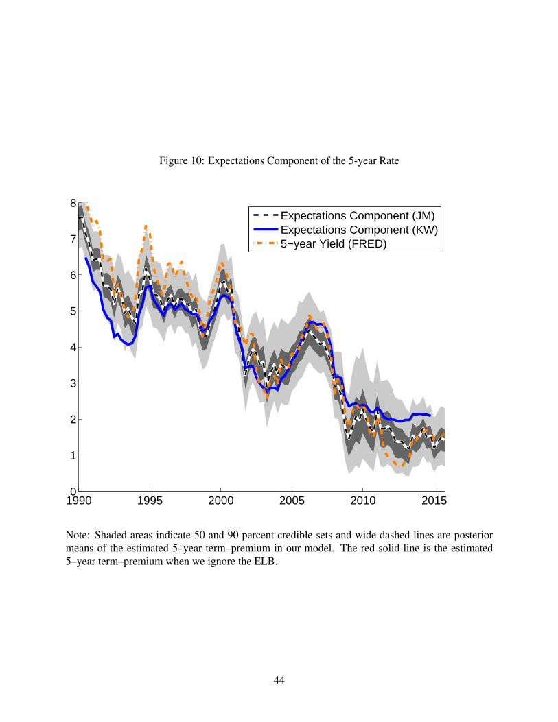
Figure 10: Expectations Component of the 5-year Rate

1990 1995 2000 2005 2010 20150

1

2

3

4

5

6

7

8Expectations Component (JM)Expectations Component (KW)5−year Yield (FRED)

Note: Shaded areas indicate 50 and 90 percent credible sets and wide dashed lines are posteriormeans of the estimated 5–year term–premium in our model. The red solid line is the estimated5–year term–premium when we ignore the ELB.

44

Table 1: Forecast Evaluation (Through 2007)

Forecast horizon h

1 2 3 4 8

Panel A: Short-term interest rate it+h

baseline

RMSE 0.33 0.69 1.02 1.34 2.20MAD 0.25 0.53 0.81 1.08 1.78PS 0.58 −0.69 −1.37 −1.86 −2.81

ELB ignored

rel. RMSE 1.00 1.00 1.00 1.00 1.00rel. MAD 1.00 1.00 1.00 1.00 1.00rel. PS −0.99∗∗∗ −0.44∗∗∗ −0.15∗∗ 0.02 0.33∗∗∗

without medium-term yield

rel. RMSE 1.12∗∗ 1.06 1.02 1.00 0.98rel. MAD 1.11∗ 1.04 1.00 0.97 0.98rel. PS −0.15∗∗∗ 0.01 0.05 0.07 0.06

Panel B: Long-term interest rate yt+h

baseline

RMSE 0.45 0.73 0.91 1.09 1.40MAD 0.37 0.61 0.74 0.89 1.10PS 0.22 −0.65 −1.06 −1.37 −1.92

ELB ignored

rel. RMSE 1.00 1.00 1.00 1.00 1.00rel. MAD 1.00 1.00 1.00 1.00 1.00rel. PS −0.89∗∗∗ −0.49∗∗∗ −0.31∗∗∗ −0.20∗∗∗ 0.02

Note: RMSE are root-mean-squared errors computed from using each the means of each model’spredictive densities as forecasts; MAD are mean absolute deviations obtained from using the me-dians of each model’s predictive densities. PS are average predictive scores. Relative RMSEand MAD are expressed as ratios relative to the corresponding statistics from the baseline model(values below unity denoting better performance than baseline); predictive scores are expressedas differences relative to the baseline (positive values denoting better performance than baseline).Predictive densities are re-estimated over growing samples that all start in 1960:Q1. For the fore-cast evaluation, the first forecast jumps off in 1984:Q4 and the last in 2007:Q4. Stars indicatesignificant differences, relative to baseline, in squared losses, absolute losses and density scores,respectively, as assessed by the test of Diebold and Mariano (1995); ∗∗∗, ∗∗ and ∗ denote signifi-cance at the 1%, 5% respectively 10% level.

45

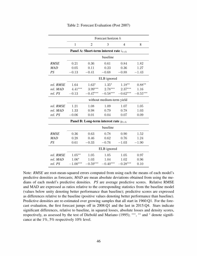
Table 2: Forecast Evaluation (Post 2007)

Forecast horizon h

1 2 3 4 8

Panel A: Short-term interest rate it+h

baseline

RMSE 0.21 0.36 0.61 0.84 1.82MAD 0.05 0.11 0.23 0.36 1.27PS −0.13 −0.41 −0.68 −0.88 −1.43

ELB ignored

rel. RMSE 1.64 1.63∗ 1.35∗ 1.18∗∗ 0.88∗∗

rel. MAD 4.41∗∗∗ 3.99∗∗∗ 2.78∗∗∗ 2.37∗∗∗ 1.16rel. PS −0.13 −0.47∗∗∗ −0.58∗∗∗ −0.62∗∗∗ −0.55∗∗∗

without medium-term yield

rel. RMSE 1.21 1.08 1.09 1.07 1.05rel. MAD 1.33 0.98 0.79 0.78 1.03rel. PS −0.06 0.01 0.04 0.07 0.09

Panel B: Long-term interest rate yt+h

baseline

RMSE 0.36 0.63 0.78 0.90 1.52MAD 0.28 0.46 0.62 0.76 1.24PS 0.61 −0.33 −0.76 −1.03 −1.90

ELB ignored

rel. RMSE 1.05∗∗ 1.05 1.05 1.05 0.97rel. MAD 1.06∗ 1.03 1.04 1.02 0.96rel. PS −1.00∗∗∗ −0.59∗∗∗ −0.40∗∗∗ −0.28∗∗∗ 0.10

Note: RMSE are root-mean-squared errors computed from using each the means of each model’spredictive densities as forecasts; MAD are mean absolute deviations obtained from using the me-dians of each model’s predictive densities. PS are average predictive scores. Relative RMSEand MAD are expressed as ratios relative to the corresponding statistics from the baseline model(values below unity denoting better performance than baseline); predictive scores are expressedas differences relative to the baseline (positive values denoting better performance than baseline).Predictive densities are re-estimated over growing samples that all start in 1960:Q1. For the fore-cast evaluation, the first forecast jumps off in 2008:Q1 and the last in 2015:Q4. Stars indicatesignificant differences, relative to baseline, in squared losses, absolute losses and density scores,respectively, as assessed by the test of Diebold and Mariano (1995); ∗∗∗, ∗∗ and ∗ denote signifi-cance at the 1%, 5% respectively 10% level.

46

a time series model of interest rates with the effective ... · a time series model of interest...

Documents