a three-step wavelet galerkin method for parabolic and hyperbolic partial differential equations

8/13/2019 A Three-step Wavelet Galerkin Method for Parabolic and Hyperbolic Partial Differential Equations

http://slidepdf.com/reader/full/a-three-step-wavelet-galerkin-method-for-parabolic-and-hyperbolic-partial-differential 1/16

International Journal of Computer MathematicsVol. 83, No. 1, January 2006, 143–157

A three-step wavelet Galerkin method for parabolic andhyperbolic partial differential equations

B. V. RATHISH KUMAR* and MANI MEHRA

Department of Mathematics, Indian Institute of Technology, Kanpur, India

(Received 11 November 2004; in nal form 2 February 2005)

A three-step waveletGalerkin methodbased onTaylor series expansion in time is proposed. Theschemeis third-order accurate in time and O( 2− jp ) accurate in space. Unlike Taylor–Galerkin methods, thepresent scheme does not contain any new higher-order derivatives which makes it suitable for solvingnon-linear problems. The compactly supported orthogonal wavelet bases D6 developed by Daubechiesare used in the Galerkin scheme. The proposed scheme is tested with both parabolic and hyperbolicpartial differential equations. The numerical results indicate the versatility and effectiveness of theproposed scheme.

Keywords : Three-step method; Wavelets; Parabolic equation; Hyperbolic equation

C.R. Category : G.1.8

1. Introduction

Wavelet analysis is a new numerical concept which allows one to represent a function in termsof a set of basis functions, called wavelets, which are localized in space. As we have notedearlier, spectral bases are innitely differentiable but have global support. On the other hand,basis functions used in nite-element methods have small compact support but poor continu-ity properties. As a result, spectral methods have good spectral localization but poor spatiallocalization, while nite element methods have good spatial localization, but poor spectrallocalization. Wavelet bases appear to combine the advantages of both spectral and nite ele-ment bases. We can expect numerical methods based on wavelet bases to be able to attaingood spatial and spectral resolution.

Recently much effort has been put into developing schemes based on the properties of orthonormal wavelet bases introduced in the 1980s by Stromberg and Meyer. These bases areformed by the dilation and translation of a single function ψ(x) , ψ j,k (x) = 2− j / 2ψ( 2j x − k) ,where j, k ∈ Z . Then for certain ψ(x) , the sequence of functions (ψ j,k (x)) (j,k) ∈ Z 2 formsan orthonormal basis in L2(R) . In wavelet applications to the solution of partial differentialequations(PDEs) themost frequentlyused wavelets are those with compact support introduced

*Corresponding author. Email: [email protected]

International Journal of Computer MathematicsISSN 0020-7160 print / ISSN 1029-0265 online © 2006 Taylor & Francis

http: // www.tandf.co.uk / journalsDOI: 10.1080 / 00207160500112985



144 B. V. Rathish Kumar and M. Mehra

by Daubechies [1]. Exploration of the usage of Daubechies wavelets to solve PDEs has beenundertaken by a number of investigators [2–5] . In another useful approach wavelets are used todrive the adaptive nite-difference method, as advocated by Jameson [6], and this applicationhas been established in a series of papers [7–9].

In the conventional numerical approach to transient problems the accuracy gained by usingthe high-order spatial discretization is partially lost because of the use of low-order timediscretization schemes. Here, spatial approximation usually precedes temporal discretization.However, the reversed order of discretization can lead to better time accurate schemes withimproved stability properties. The fundamental idea behind theTaylor–Galerkin approach [10]is the substitution of space derivatives for the time derivatives in the Taylor series, as used in thederivation of the Lax–Wendroff method [11], the only modication being that the procedureis carried out to third order. However, its applications are mainly to hyperbolic problems andsome convection diffusion equations because too many terms are introduced in the third-ordertime derivative term, especially for non-linear multidimensional equations, and treatment of

the boundary integrations arising from high-order time derivative terms is too complicated.A three-step nite-element method based on a Taylor series expansion in time is proposed

in [12]. This scheme involves neither complicated expression nor higher-order derivativesas in the wavelet Taylor–Galerkin method [13] and the wavelet multilayer Taylor–Galerkinmethod [14]. In [13] we investigated the feasibility of applying the new wavelet Taylor–Galerkin to an important application problem of the Korteweg–de Vires (KdV) equation. Acombination of such a time marching scheme with wavelet approximation in space can leadto simple higher-order space and time accurate numerical methods. In this paper we developa three-step wavelet Galerkin method (T-WGM) for a class of linear problems such as theheat equation, the convective transport problem and the non-linear Burgers equation in one

dimension and the heat equation in twodimensions. This schemeretains thegood accuracy andstability properties of the Taylor–Galerkin method without needing to calculate higher-orderderivative terms.

Theoutline of paper is asfollows. In section2 wesummarizesome basicsof waveletanalysis.In section 3 we consider the application of T-WGM to the heat equation, the convectionequation and the non-linear Burgers equation. In section 4 we study stability of the algorithmin the context of ODEs. Numerical results are given in section 5. In section 6 we extendT-WGM to the heat equation in two dimensions. Finally, in section 7 we draw a number of conclusions based on our results.

2. Wavelet preliminaries

2.1 Compactly supported wavelets

Daubechies [1] has dened the class of compactly supported wavelets. Briey, let φ be asolution of the scaling relation

φ(x) =k

a kφ( 2x − k)

where the ak are a collection of coefcients that categorize the specic wavelet basis. Theexpression φ is called the scaling function. The associated wavelet function ψ is dened bythe equation

ψ(x) =k

(− 1)ka 1− kφ( 2x − k).



Three-step wavelet method 145

Normalization φ dx = 1 of the scaling function leads to the condition

k

a k = 2.

The translates of φ are required to be orthonormal, i.e.

φ(x − k)φ(x − m) dx = δk,m .

The scaling relation implies the condition

N − 1

k= 0

a ka k− 2m = δ0,m

where N is the order of wavelet. For coefcients verifying the above two conditions, thefunctions consisting of translates and dilations of the wavelet function ψ( 2j x − k) form acomplete orthogonal basis for square integrable functions on the real line L 2(R) .

If only a nite number of the ak are non-zero, φ will have compact support. Since

φ(x)ψ(x − m) dx =k

(− 1)ka1− ka k− 2m = 0

the translates of the scaling function and wavelet dene orthogonal subspaces

V j = { 2j / 2φ( 2j x − k) ; m = . . . , − 1, 0, 1, . . . }

W j = { 2j / 2ψ( 2j x − k) ; m = . . . , − 1, 0, 1, . . . }.

The relation

V j + 1 = V j + W j

implies the Mallat transform [1]

V 0 ⊂ V 1 ⊂ · · · ⊂ V j + 1

V j + 1 = V 0 ⊕ W 0 ⊕ W 1 ⊕ · · ·⊕ W j .

Smooth scaling functions arise as a consequence of the degree of approximation of the trans-lates. The result that the polynomials 1 , x , . . . , x p − 1 are expressed as linear combinations of the translates of φ (x − k) is implied by the conditions

k

(− 1)− kkm a k = 0

for m = 0, 1, . . . , p − 1. The following are equivalent results:

• {1, x , . . . , x p − 1} are linear combinations of φ (x − k)• f − c j

k φ( 2j x − k) ≤ C 2− jp f p , where cj k =

f (x)φ( 2j x − k) dx

•

xm ψ(x) dx = 0 for m = 0, 1, . . . , p − 1

• f (x)ψ( 2j x) dx ≤ c2− jp .

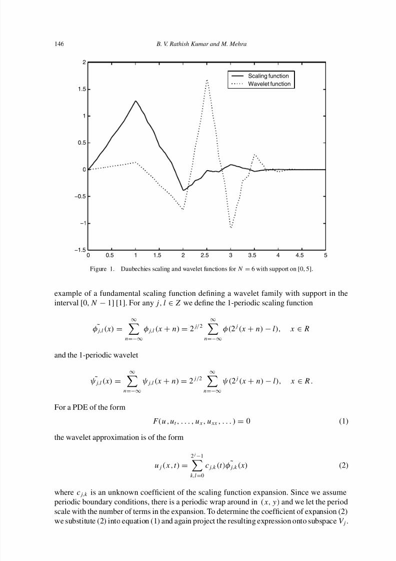
For the Daubechies scaling / wavelet function DN , we have p = N / 2 where N is the orderof the wavelet. Figure 1 shows an example of a compactly supported scaling function andits associated fundamental wavelet function. For arbitrarily large even N there is Daubechies




0 0.5 1 1.5 2 2.5 3 3.5 4 4.5 5−1.5

−1

−0.5

0

0.5

1

1.5

2

Scaling functionWavelet function

Figure 1. Daubechies scaling and wavelet functions for N = 6 with support on [0, 5].

example of a fundamental scaling function dening a wavelet family with support in theinterval [0, N − 1] [1]. For any j , l ∈ Z we dene the 1-periodic scaling function

˜φ j,l (x) =∞

n=−∞

φ j,l (x + n) = 2j/ 2∞

n=−∞

φ( 2 j (x + n) − l), x ∈ R

and the 1-periodic wavelet

˜ψ j,l (x) =∞

n=−∞

ψ j,l (x + n) = 2j / 2∞

n=−∞

ψ( 2j (x + n) − l), x ∈ R .

For a PDE of the form

F(u,u t , . . . , u x , u xx , . . . ) = 0 (1)

the wavelet approximation is of the form

u j (x,t) =2 j − 1

k,l = 0

cj,k (t) ˜φ j,k (x) (2)

where cj,k is an unknown coefcient of the scaling function expansion. Since we assumeperiodic boundary conditions, there is a periodic wrap around in (x, y) and we let the periodscale with the number of terms in the expansion. To determine the coefcient of expansion (2)we substitute (2) into equation (1) and again project the resulting expression onto subspace V j .




The projection requires cj,k to satisfy the equation

∞

−∞

˜φ j,m (x)F(u j , u j t , u j x , u j xx , . . . ) dx = 0.

To evaluate this expression we must know the coefcients of the form

∧(l 1 , l 2 , . . . , l n , d 1 , d 2 , . . . , d n ) = ∧ d 1d 2 ··· d nl1 l2 ··· ln

= ∞

−∞

n

i = 1

φ̃ d ili

(y) dy = ∞

−∞

n

i = 1

φ d ili

(y) dy.

Since the scaling function used to dene compact wavelets has a limited number of deriva-tives, the numerical evaluation of these expressions is often unstable or inaccurate. A specialalgorithm to evaluate the connection coefcients has been devised by Latto et al. [15].

2.2 Multivariate wavelets

The simplest way to obtain multivariate wavelets is to employ anisotropic or isotropic tensorproducts.

MRA-d Here, the multivariate wavelets are dened by

ψ j,l (x) := ψ j 1 ,l 1 (x 1) , . . . , ψ j d ,l d (x d ), j := (j 1 , . . . , j d ) x, l analogous .

MRA Here, anisotropy is avoided.The scaling functions are simply the tensor products of theunivariate scaling functions. A two-dimensional MRA can be constructed from the followingdecomposition:

V j = V j ⊗ V j = (V j − 1 ⊕ W j − 1) ⊗ (V j − 1 ⊕ W j − 1)

= (W j − 1 ⊗ W j − 1) ⊕ (W j − 1 ⊗ V j − 1) ⊕ (V j − 1 ⊗ W j − 1) ⊕ V j − 1 ⊗ V j − 1

= W j − 1 ⊕ V j − 1 .

Then we have V J = W J − 1 ⊕ · · ·⊕ W 0 ⊕ V 0 and the wavelet basis is given by

{ψ j,k ⊗ ψ j,l , ψ j,k ⊗ φ j,l , φ j,k ⊗ ψ j,l }k,l ∈Z, 0≤ j ≤ J − 1 ∪ {φ0,k ⊗ φ0,l }k,l ∈Z .

We have used this MRA approach in our two dimensional problem.

3. Three-step wavelet Galerkin method

Before introducing the three-step wavelet Galerkin method (T-WGM), it is necessary to give abrief statement of the two-step Lax–Wendroff wavelet Galerkin method (L-WGM). Considerthe equation

u t = L u + N f(u) (3)




with the initial condition

u(x, 0) = u 0(x), 0 ≤ x ≤ 1 (4)

and with suitable boundary conditions.We explicitly separate equation (3) intoa linear part L uand non-linear part N f(u) , where the operations L and N are constant-coefcient differentialoperation that do not depend upon time t . The function f(u) is non-linear. Performing a Taylorseries expansion in time, we have

u(t + t) = u(t) + t ∂u(t)

∂t +

t 2

2∂2u(t)

∂t 2 +

t 3

6∂3u(t)

∂t 3 + O( t 4). (5)

By approximating equation (5) to second-order accuracy, the formulation of the two-stepmethod can be derived as follows:

u t +

t

2 = u(t) +

t

2

∂u(t)

∂t

u(t + t) = u(t) + t ∂u(t + ( t/ 2))

∂t .

(6)

Spatial discretization of equations (6) can be performed using the WGM. We will call thismethod L-WGM.

Now we introduce the three-step wavelet Galerkin method. By approximating equation (5)up to third-order accuracy, the formulation of the three-step method can be written as follows:

u t +t

3 = u(t) +

t

3

∂u(t)

∂t

u t +t 2

= u(t) +t 2

∂u(t + ( t/ 3))∂t

u(t + t) = u(t) + t ∂u(t + ( t/ 2))

∂t .

(7)

Spatial discretization of equations (7) can be performed using the WGM. In contrast with theTaylor–Galerkinmethod, theT-WGMdoesnot contain anynewhigher-order spatial derivativesand thus can easily be used to solve non-linear multidimensional ows.

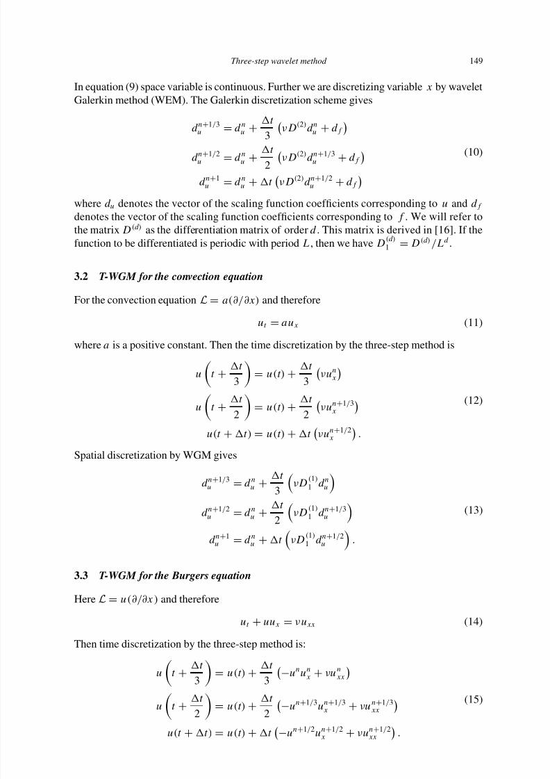
3.1 T-WGM for the heat equation

For the heat equation L = ν (∂ 2 /∂ 2x ) and therefore

u t = νu xx + f(x) (8)

where ν is a positive constant. Let us rst keep the spatial variable x continuous and discretizethe time by the three-step method:

u t +t

3 = u(t) +

t

3νu n

xx + f(x)

u t +t 2

= u(t) +t 2

νu n+ 1/ 3xx + f(x)

u(t + t) = u(t) + t νu n+ 1/ 2xx + f(x) .

(9)




Spatial discretization by WGM gives

d n+ 1/ 3u = d nu +

t

3

− 23j / 2

k m

(c j k )n (c j

m )n∧

001lkm + ν( 2j )2

k

(c j k )n∧

02lk

d n+ 1/ 2u = d nu +

t 2

− 23j / 2

k m

(c j k )n+ 1/ 3(c j

m )n+ 1/ 3∧

001lkm + ν( 2j )2

k

(c j k )n+ 1/ 3

∧02lk

d n+ 1u = d nu + t − 23j / 2

k m

(c j k )n+ 1/ 2(c j

m )n+ 1/ 2∧

001lkm + ν( 2j )2

k

(c j k )n+ 1/ 2

∧02lk .

(16)

4. Theoretical stability of the linearized schemes

We use the concept of asymptotic stability of a numerical method as dened in [17] for adiscrete problem of the form

dU dt

= LU

where L is assumed to be a diagonalizable matrix. The most crucial property of L is itsspectrum, for this will determine the stability of time discretization. If the spatial discretizationis presumed to be xed, then we use the term stability in its ODE context.

DEFINITION The region of absolute stability of a numerical method is dened for the scalar model problem

dU dt

= λU

to be the set of all λ t such that || U n || is bounded as t → ∞ .

Finally we say that a numerical method is asymptotically stable for a particular problemif, for sufciently small t > 0, the product of t and every eigenvalue of L lies within theregion of absolute stability.

5. Results of numerical experiments

In this section we solve PDEs with periodic boundary conditions and initial condition u 0(x) . Aheat equation, a linear convection equation and a non-linear Burgers equation are consideredin one dimension. All the results are presented using Daubechies D 6 scaling function. Theerror produced by the numerical schemes was measured against the values of the analytical

solution u e by the L ∞ norm calculated as

u L ∞ = maxk= 0, 1,..., 2 j − 1

u k2j

.




Table 1. Accuracy of results given by the L ∞ norm.

j t Lax–Wendroff WGM L-WGM T-WGM

4 0.0005 (0.01) 3 .178 × 10− 6 3.138 × 10− 7 2.2884 × 10− 11 1.6209 × 10− 11

6 0.0005 (0.01) 3 .142 × 10− 6 3.138 × 10− 7 6.5721 × 10− 12 1.0299 × 10− 137 0.0005 (0.01) 3 .142 × 10− 6 3.138 × 10− 7 6.5721 × 10− 12 1.0299 × 10− 13

5.1 Heat equation

We have tested T-WGM on a heat equation with u 0(x) = 0 and f (x) = sin (2πx) . Errors inthe L∞ norm of the solution obtained by Lax–Wendroff, WGM using Euler time stepping,L-WGM and T-WGM are compared in table 1. In the table the notation x(y) means that thetarget time y is reached by time marching with a step size of x .

5.2 Convection equation

The accuracy of the proposed T-WGM for hyperbolic problems has been veried numericallyon the classical test problem of convection with a Gaussian prole. We assume that the solutionis periodic with some large period, say 4. The solutions obtained by WGM using Euler timestepping, L-WGM and T-WGM are compared in table 2. For stability analysis of L-WGM,L j is the matrix dened by

L j = aD (1) +a 2 t

2D (2) ,

and for T-WGML j = aD (1) +

a 2 t 2

D (2) +a 3 t 2

6D (3) .

For j = 4, we have found by stability analysis that t ≤ 0.00835.Regions of absolute stabilityfor T-WGM are plotted in gure 2.

5.3 Burgers equation

The analytical solution to equation (14) with the initial condition u0(x) after using the Cole–Hopf transformation is given by

u(x,t) = ∞

−∞ (x − ξ)/t exp − (x − ξ ) 2 / 4νt exp − (2ν) − 1

ξ

0 uo (η) dη dξ

∞

−∞ exp − (x − ξ ) 2 / 4νt exp − (2ν) − 1 ξ

0 u0(η) dη dξ . (17)

We have integrated equation (17) numerically using Gauss–Hermite quadrature in order todetermine the accuracy of our method.

Table 2. Accuracy of results given by the L ∞ norm.

j t WGM L-WGM T-WGM

4 0.01 (0.5) 0.0861 0.0014 0.00126 0.001 (0.5) 0.0021 2 .042 × 10− 5 3.94 × 10− 7

6 0.0001 (0.5) 0.0002 3 .7881 × 10− 7 3.70 × 10− 7




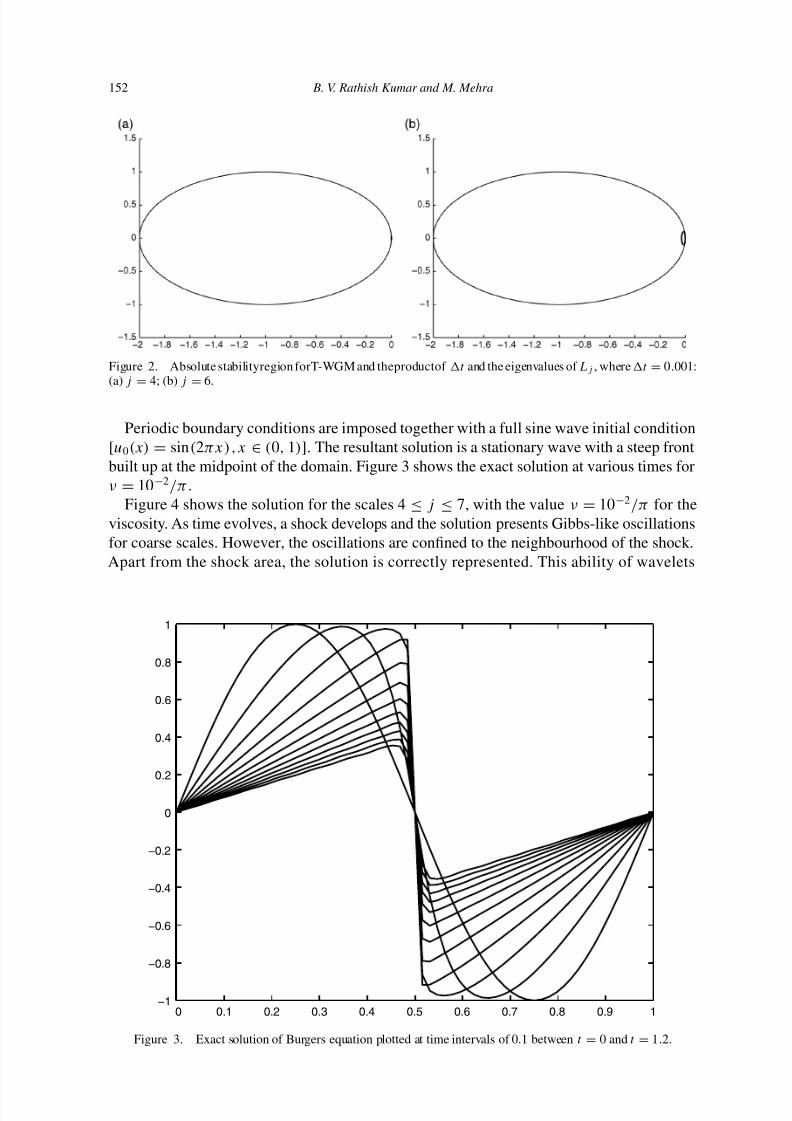
Figure 2. Absolute stabilityregion forT-WGM and theproductof t and the eigenvalues of L j , where t = 0.001:(a) j = 4; (b) j = 6.

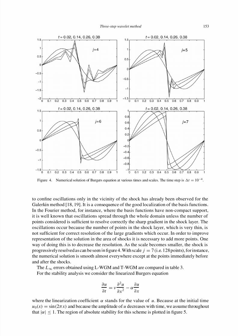
Periodic boundary conditions are imposed together with a full sine wave initial condition[u 0(x) = sin (2πx),x ∈ (0, 1)]. The resultant solution is a stationary wave with a steep frontbuilt up at the midpoint of the domain. Figure 3 shows the exact solution at various times forν = 10 − 2 /π .

Figure 4 shows the solution for the scales 4 ≤ j ≤ 7, with the value ν = 10− 2 /π for theviscosity. As time evolves, a shock develops and the solution presents Gibbs-like oscillationsfor coarse scales. However, the oscillations are conned to the neighbourhood of the shock.Apart from the shock area, the solution is correctly represented. This ability of wavelets

0 0.1 0.2 0.3 0.4 0.5 0.6 0.7 0.8 0.9 1−1

−0.8

−0.6

−0.4

−0.2

0

0.2

0.4

0.6

0.8

1

Figure 3. Exact solution of Burgers equation plotted at time intervals of 0.1 between t = 0 and t = 1.2.




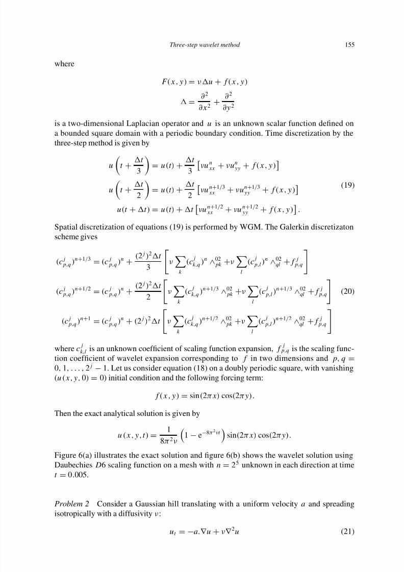
Figure 4. Numerical solution of Burgers equation at various times and scales. The time step is t = 10− 4 .

to conne oscillations only in the vicinity of the shock has already been observed for theGalerkin method [18, 19]. It is a consequence of the good localization of the basis functions.In the Fourier method, for instance, where the basis functions have non-compact support,it is well known that oscillations spread through the whole domain unless the number of points considered is sufcient to resolve correctly the sharp gradient in the shock layer. Theoscillations occur because the number of points in the shock layer, which is very thin, is

not sufcient for correct resolution of the large gradients which occur. In order to improverepresentation of the solution in the area of shocks it is necessary to add more points. Oneway of doing this is to decrease the resolution. As the scale becomes smaller, the shock isprogressively resolvedas can beseen in gure 4.With scale j = 7 (i.e. 128points), for instance,the numerical solution is smooth almost everywhere except at the points immediately beforeand after the shocks.

The L ∞ errors obtained using L-WGM and T-WGM are compared in table 3.For the stability analysis we consider the linearized Burgers equation

∂u∂t

= ν∂2u

∂x 2 − α∂u∂x

where the linearization coefcient α stands for the value of u. Because at the initial timeu 0(x) = sin (2πx) and because the amplitude of u decreases with time, we assume throughoutthat |α | ≤ 1. The region of absolute stability for this scheme is plotted in gure 5.




Table 3. Accuracy of results given by the L ∞norm.

j t Time t L-WGM T-WGM

4 10− 3

0.02 0.0112 0.01120.14 0.1557 0.15570.26 0.6828 0.68280.38 0.6953 0.6953

5 10− 3 0.02 0.0046 0.00460.14 0.0476 0.04750.26 0.4724 0.47250.38 0.3674 0.3674

6 10− 3 0.02 0.0016 0.00160.14 0.0114 0.01140.26 0.2120 0.21200.38 0.1546 0.1546

7 10− 3 0.02 0.0005 0.00050.14 0.0049 0.00500.26 0.0500 0.05000.38 0.0418 0.0418

Figure 5. Absolute stability region for (a) forward Euler and the product of t and the eigenvalues of L 7 and (b)the product of t and the eigenvalues of L 7 , for D = 6, where t = 10− 3 , α = 1 and ν = 10− 2 /π .

6. Extension to multidimensional problems

Theschemes developed in thepreceding sections for a one-dimensionalproblems havedemon-strated the value of T-WGM compared with WGM and L-WGM. However, to be of practicalinterest T-WGM should also be applicable to multidimensional problems. To show that this isindeed the case, we consider the problem of heat conduction and the standard test problemsof hill translation in two dimensions.

Problem 1 Heat conduction problem

∂u∂t

= F (x,y) (18)




where

F(x,y) = ν u + f(x,y)

= ∂2

∂x 2 + ∂2

∂y 2

is a two-dimensional Laplacian operator and u is an unknown scalar function dened ona bounded square domain with a periodic boundary condition. Time discretization by thethree-step method is given by

u t +t 3

= u(t) +t 3

νu nxx + νu n

yy + f(x,y)

u t +t 2

= u(t) +t 2

νu n+ 1/ 3xx + νu n+ 1/ 3

yy + f(x,y)

u(t + t) = u(t) + t νu n+ 1/ 2xx + νu n+ 1/ 2

yy + f(x,y) .

(19)

Spatial discretization of equations (19) is performed by WGM. The Galerkin discretizatonscheme gives

(c j p,q )n+ 1/ 3 = (c j

p,q )n +(2j )2 t

3ν

k

(c j k,q )n

∧02pk + ν

l

(c j p,l )n

∧02ql + f j

p,q

(c j p,q )n+ 1/ 2 = (c j

p,q )n +(2j )2 t

2

νk

(c j k,q )n+ 1/ 3

∧02pk + ν

l

(c j p,l )n+ 1/ 3

∧02ql + f j

p,q (20)

(c j p,q )n+ 1 = (c j

p,q )n + (2j )2 t νk

(c j k,q )n+ 1/ 2

∧02pk + ν

l

(c j p,l )n+ 1/ 2

∧02ql + f j

p,q

where c j k,l is an unknown coefcient of scaling function expansion, f j

p,q is the scaling func-tion coefcient of wavelet expansion corresponding to f in two dimensions and p, q =0, 1, . . . , 2j − 1. Let us consider equation (18) on a doubly periodic square, with vanishing(u(x,y, 0) = 0) initial condition and the following forcing term:

f(x,y) = sin (2πx) cos (2πy).

Then the exact analytical solution is given by

u(x,y,t) =1

8π 2ν1 − e− 8π 2 νt sin (2πx) cos (2πy).

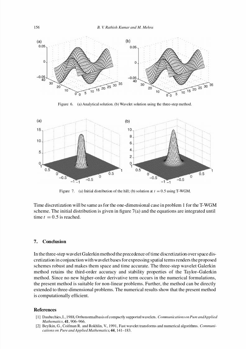
Figure 6(a) illustrates the exact solution and gure 6(b) shows the wavelet solution usingDaubechies D 6 scaling function on a mesh with n = 25 unknown in each direction at timet = 0.005.

Problem 2 Consider a Gaussian hill translating with a uniform velocity a and spreadingisotropically with a diffusivity ν :

u t = − a. ∇ u + ν∇ 2u (21)




Figure 6. (a) Analytical solution. (b) Wavelet solution using the three-step method.

Figure 7. (a) Initial distribution of the hill; (b) solution at t = 0.5 using T-WGM.

Time discretization will be same as for the one-dimensional case in problem 1 for the T-WGMscheme. The initial distribution is given in gure 7(a) and the equations are integrated untiltime t = 0.5 is reached.

7. Conclusion

In the three-step wavelet Galerkin method the precedence of time discretization over space dis-cretization in conjunction with wavelet bases for expressing spatial terms renders the proposedschemes robust and makes them space and time accurate. The three-step wavelet Galerkinmethod retains the third-order accuracy and stability properties of the Taylor–Galerkinmethod. Since no new higher-order derivative term occurs in the numerical formulations,the present method is suitable for non-linear problems. Further, the method can be directlyextended to three-dimensional problems. The numerical results show that the present methodis computationally efcient.

References[1] Daubechies, I., 1988, Orthonormalbasis of compactly supported wavelets. Communicationson Pure andApplied

Mathematics , 41 , 906–966.[2] Beylkin, G., Coifman R. and Rokhlin, V., 1991, Fast wavelet transforms and numerical algorithms. Communi-

cations on Pure and Applied Mathematics , 44 , 141–183.




[3] Glowinski, R., Lawton, W., Ravachol, M. and Tenenbaum, E., 1990, Wavelet solutions of linear and non-linearelliptic, parabolic andhyperbolic problemsin ID. In:R. Glowinski (Ed.) Computing Methods in AppliedSciencesand Engineering , pp. 55–120 (Philadelphia, PA: SIAM).

[4] Latto, A. and Tenenbaum, E., 1990, Compactly supported wavelets and the numerical solution of Burgers’equation. Comptes Rendus, French Academy of Science, Series I , 311 , 903–909.

[5] Qian, S. and Weiss, J., 1992, Wavelets and the numerical solution of partial differential equations. Journal of Computational Physics , 106 , 155–175.

[6] Jameson, L., 1998, A wavelet-optimized very high order adaptive grid and order numerical method. SIAM Journal on Scientic Computing , 19 , 1980–2013.

[7] Holmstrom, M., 1999, Solving hyperbolic PDEs using interpolating wavelets. SIAM Journal on ScienticComputing , 21 , 405–420.

[8] Holmstrom, M., and Walden, J., 1998, Adaptive wavelets methods for hyperbolic PDEs. Journal of ScienticComputing , 13 , 19–49.

[9] Fatkulin, I. andHesthaven,J.S.,2001,Adaptive high-order nite-differencemethod fornonlinear waveproblems. Journal of Scientic Computing , 16 , 47–67.

[10] Donea, J., 1984, A Taylor–Galerkin method for convective transport problems. International Journal for Numerical Methods in Engineering , 20 , 101–119.

[11] Lax, P.D. and Wendrof, B., 1960, Systems of conservation laws. Communications on Pure and Applied Mathematics , 13 , 217.

[12] Jiang, C.B.andKawahara, M., 1993, Theanalysisof unsteadyincompressibleows by a three-step nite elementmethod. International Journal for Numerical Methods in Fluids , 16 , 793–811.

[13] Rathish Kumar, B.V. and Mehra, M., 2004, Time accurate solutionof Korteweg–deVries equationusing waveletGalerkin method. Applied Mathematics and Computation , 162 , 447–460.

[14] Rathish Kumar, B.V. and Mehra, M., 2005, Wavelet multilayer Taylor Galerkin schemes for hyperbolic andparabolic problems. Accepted for publication in Applied Mathematics and Computation. Available online at:http: // authors.elsevier.com / sd/ article / S0096300304004394 (accessed 4 May 2005).

[15] Latto, A., Resnikoff, H.L. and Tenenbaum, E., 1991, The evaluation of connection coefcients of compactlysupported wavelets. In: Proceedings of the French–USA Workshop on Wavelets and Turbulence, Princeton, 1991(New York: Springer-Verlag).

[16] Nilsen, O.M., 1998, Wavelets in scientic computing. PhD thesis, Technical University of Denmark, Lyngby.[17] Canute, C., Hussaini, M.Y., Quarteroni, A. and Zang, T.A., 1988, Spectral Methods in Fluid Dynamics (New

York: Springer-Verlag)

[18] Liandrat, J. and Tchamitchian, Ph., 1990, Resolution of the 1-D regularised Burgers equation using spatialwavelet approximation algorithm and numerical results. Technical Report 90-83. ICASE, NASA LangleyResearch Center.

[19] Avudainayagam, A. and Vani, C., 1999, Wavelet-Galerkin solutions of quasilinear hyperbolic conservationequations. Communications in Numerical Methods in Engineering , 15 , 589–601.

a three-step wavelet galerkin method for parabolic and hyperbolic partial differential equations

Documents