Partition Analysis and Ehrhart Theory

A thesis presented to the faculty ofSan Francisco State University

In partial fulfilment ofThe requirements for

The degree

Master of ArtsIn

Mathematics

byDorothy L. Moorefield

San Francisco, CAJanuary 2007

Copyright byDorothy L. Moorefield

2007

CERTIFICATION OF APPROVAL

I certify that I have read Partition Analysis and Ehrhart Theory by Dorothy L. Moorefield

and that in my opinion this work meets the criteria for approving a thesis submitted in

partial fulfillment of the requirements for the degree: Master of Arts in Mathematics at

San Francisco State University.

Matthias BeckProfessor of Mathematics

Joseph GubeladzeProfessor of Mathematics

Serkan HostenProfessor of Mathematics

Partition Analysis and Ehrhart Theory

San Francisco State University

January, 2007

Dorothy L. Moorefield

ABSTRACT

In the early 1900s, Major Percy A. MacMahon developed the ! Operator as

a tool for enumerating partitions via their corresponding diophantine rela-

tions. In this paper, we will give an introduction to MacMahon’s techniques

provided in his now classic Combinatory Analysis. Then we will show how

MacMahon’s methods can be applied to the problem of enumerating lattice

points in polyhedra. Corteel, Lee and Savage have developed five guidelines

that provide a simplification of MacMahon’s partition analysis for integral,

linear, homogeneous systems of inequalities. We will discuss these guide-

lines and then expand on them to include linear systems of equalities in the

e"ort to find the Ehrhart polynomial for faces of the Birko" polytope.

I certify that the Abstract is a correct representationof the content of this thesis.

Matthias BeckChairperson, Advisory Committee

ACKNOWLEDGEMENTS

First and foremost I would like to thank Dr. Matthias Beck for being an

awesome advisor. I would also like to thank my committee members Dr.

Serkan Hosten and Dr. Joseph Gubeladze for their excellent suggestions.

I would like to give a special thanks to Eric Tong for providing me with a

quiet place to work at odd hours, Quan Le for doing all work to get this

thesis submitted in my absence and his Latex expertise, and finally Daimhin

Murphy for providing encouragement and support throughout my Master’s

career.

v

Contents

1. A Beginning 1

2. Ehrhart Theory 2

2.1. Introduction 2

2.2. Generating Functions 4

2.3. Overview of Current Methods 6

2.4. The Birko" and Chan-Robbins-Yuen Polytopes 12

3. MacMahon’s Partition Analysis 15

3.1. Introduction 15

3.2. Definition of !! and Identities 15

3.3. Definition of != and Identities 19

3.4. Formal vs. Analytic 21

4. Partition Analysis and Polytopes 23

4.1. Introduction 23

4.2. The General Idea 23

4.3. Partition Analysis and CYR 28

5. On the Hunt for a New Algorithm 32

5.1. Introduction 32

5.2. Symmetric Functions 32

5.3. Switching Gears 36

5.4. Five Guidelines for !! 37

5.5. Guidelines for != 41

6. Future Work 43

References 44

vi

1. A Beginning

In the introduction to the second volume of Combinatory Analysis [9], Major Percy A.

MacMahon states:

“In conclusion, I would say that I am aware that the reader will probably find imperfections

in the volumes, but I shall be satisfied if they are found to contain ideas which are new

and fresh, and such as are likely to prove starting-points for further investigations in an

exceedingly interesting field of pure mathematics.”

The original problem for this thesis was to find the Ehrhart polynomial of the Chan-

Robbins-Yuen polytope. While attempting to apply the traditional methods of Ehrhart

theory (outlined in chapter 2) to the given problem, the author realized the need of a dif-

ferent method of computation. This necessity lead to the study of MacMahon’s partition

analysis (outlined in chapter 3).

In the spirit of the above quote the purpose of this paper is to show means of merging

Ehrhart theory with MacMahon’s partition analysis. Even though the theories are decades

apart and arose independently, there is a significant amount of interplay between the two

in which this paper only begins to show.

1

2. Ehrhart Theory

2.1. Introduction. Let a ! Rn and b ! R. Then a hyperplane consists of the set {x !

Rn|aT x = b} and a halfspace consists of the set {x ! Rn|aT x " b}. If A is an m#n matrix

and b ! Rm then a polyhedron P consists of the set

P := {x ! Rn|Ax $ b}.

In other words, a polyhedron is the intersection of finitely many halfspaces.

If x, y ! Rn and y %= 0 then the set {x+ty|t " 0} is called a ray and the set {x+ty|t ! R}

is called a line. We say a polyhedron is bounded if it does not contain a ray. A bounded

polyhedron is called a polytope. This definition is known as the hyperplane description of

a polytope.

Let P & Rn be a polyhedron and suppose x ! P . If there exists some c ! Rn such that

for all y ! P , cT x < cT y where y %= x we say x is a vertex of P . It can be shown (refer

to [4]) that every polytope is the convex hull of it’s vertices. This leads to an alternate

definition of a polytope: A polytope is the convex hull of finitely many points. This is

known as the vertex description of a polytope.

A polytope is said to be integral if all of its vertices are integer points. If all of the

vertices of a polytope are rational points, the polytope is said to be rational.

The dimension of a polyhedron is the dimension of the a#ne space formed by the span of

the polyhedron. If P = {x ! Rn|Ax $ b} and A" be some collection of rows of A, then the

set F := P '{x ! Rn|A"x = b} is itself a polyhedron and called a face of P . The dimension

of a face F is the dimension of the span of F . If P is an n dimensional polyhedron then

2

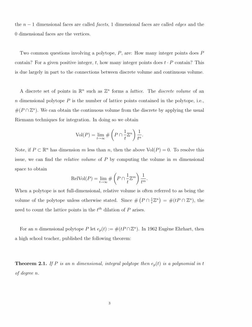
the n( 1 dimensional faces are called facets, 1 dimensional faces are called edges and the

0 dimensional faces are the vertices.

Two common questions involving a polytope, P , are: How many integer points does P

contain? For a given positive integer, t, how many integer points does t · P contain? This

is due largely in part to the connections between discrete volume and continuous volume.

A discrete set of points in Rn such as Zn forms a lattice. The discrete volume of an

n dimensional polytope P is the number of lattice points contained in the polytope, i.e.,

#(P 'Zn). We can obtain the continuous volume from the discrete by applying the usual

Riemann techniques for integration. In doing so we obtain

Vol(P ) = limt#$

#

!P ' 1

tZn

"1

tn.

Note, if P & Rn has dimension m less than n, then the above Vol(P ) = 0. To resolve this

issue, we can find the relative volume of P by computing the volume in m dimensional

space to obtain

RelVol(P ) = limt#$

#

!P ' 1

tZm

"1

tm.

When a polytope is not full-dimensional, relative volume is often referred to as being the

volume of the polytope unless otherwise stated. Since ##P ' 1

t Zn$

= #(tP ' Zn), the

need to count the lattice points in the tth dilation of P arises.

For an n dimensional polytope P let ep(t) := #(tP 'Zn). In 1962 Eugene Ehrhart, then

a high school teacher, published the following theorem:

Theorem 2.1. If P is an n dimensional, integral polytope then ep(t) is a polynomial in t

of degree n.

3

This polynomial is referred to as the Ehrhart polynomial. In Section 3 we provide a rough

sketch of the proof of Ehrhart’s theorem. For the detailed proof of Ehrhart’s theorem and

more detail of the volume of polytopes refer to [3].

2.2. Generating Functions. Let {ak}$k=0 be an infinite sequence and suppose we wish to

manipulate the sequence to perhaps find a closed formula. Then we can embed the sequence

into a generating function of the form

F (x) =$%

n=0

akxk.

Generating functions are very useful in that the degree of each monomial keeps track of

the position in the sequence while the coe#cient provides the actual value of the term.

Then if we play by the rules of either formal or analytic power series we may be able to

derive the desired result. The following is one of many nice introductory examples of the

power of generating functions provided in [3].

Consider the Fibonacci sequence f0 = 0, f1 = 1 and fk+2 = fk+1 + fk for k " 0. Let

F (x) =$%

k=0

fkxk.

Then we have$%

k=0

fk+2xk =

1

x2

$%

k=0

fk+2xk+2 =

1

x2[F (x)( x],

$%

k=0

fk+1xk =

1

x

$%

k=0

fk+1xk+1 =

1

xF (x).

Since$%

k=0

fk+2xk =

$%

k=0

(fk+1 + fk)xk =

$%

k=0

fk+1xk +

$%

k=0

fkxk,

we have1

x2[F (x)( x] =

1

xF (x) + F (x).

4

Solving for F (x) we obtain

F (x) =x

1( x( x2=

x&1( 1+

%5

2 x' &

1( 1&%

52 x

' ,

which has the following partial fraction expansion

1%5

1( 1+%

52 x

(1%5

1( 1&%

52 x

.

Now we will make use of the well known geometric series

$%

k=0

xk =1

1( x

to obtain

F (x) =1)5

$%

k=0

(1 +

)5

2x

)k

( 1)5

$%

k=0

(1(

)5

2x

)k

=$%

k=0

1)5

*

+(

1 +)

5

2

)k

((

1()

5

2

)k,

- xk.

This provides the desired closed form:

fk =1)5

*

+(

1 +)

5

2

)k

((

1()

5

2

)k,

- .

The rational function obtained using the properties of geometric series is called a ratio-

nal generating function. Often we will jump back and forth from generating functions to

rational generating functions. A natural question to ask about these generating functions

is, when are formal series appropriate as opposed to analytic series? In many cases, we

expand rational functions into their corresponding geometric series. As long as we are

living in the world of power series, we know these expansions are unique. However, as we

will see in section 4.1 when we begin to deal with Laurent series convergence becomes an

issue. In the meantime, however, we have no need to consider such things and will proceed

5

accordingly.

The main goal of the next section is to show means of finding the rational generating

function corresponding to

1 +%

t!1

#(tP ' Zn)xt,

where P is an n dimensional integral polytope. We can safely consider only positive

solutions because we can always shift a polytope into the positive orthant without changing

the lattice count. We will then show how to extract the Ehrhart polynomial and volume

of P from its rational generating function.

2.3. Overview of Current Methods. Suppose P & Rn is n dimensional. Then we say P is

a simplex if P has n + 1 vertices.

Let T be a finite collection of n dimensional simplices such that:

(1).

S'T

S = P

(2) For all Si, Sj ! T either Si ' Sj = ! or Si ' Sj is a face of both Si and Sj.

(3) Any vertex of S, where S ! T , is a vertex of P .

Then T forms a triangulation of P . A polytope P is said to be triangulated if P is

decomposed into a triangulation. Many proofs in Ehrhart theory rely on the following

theorem.

Theorem 2.2. Every polytope can be triangulated.

Let v, w1, w2, . . . , wk ! Rn. Then a cone is a set of the form

K := {v + !1w1 + !2w2 + · · · + !kwk|!i " 0}.

If K does not contain a line, then K is said to be a pointed cone where v is called the

apex and each wi is called a generator. K is said to be rational if all of its generators and

6

apex are rational. A pointed cone K & Rn is said to be simple if it has exactly n linearly

independent generators.

Suppose we have an n dimensional polytope P & Rn with vertices v1, v2, . . . , vk ! Rn.

Now consider the points in Rn+1 given by w1 = (v1, 1), w2 = (v2, 1), . . . , wk = (vk, 1). If we

use these points as generators with the origin as the apex we obtain a cone KP & Rn+1.

Notice all we are doing is lifting the polytope into a higher dimension but are not a"ect-

ing its relative volume. In other words the integer point count of the lifted polytope will

remain the same as the integer point count of the polytope. Moreover, if we slice the cone

with the hyperplane xn+1 = t, we obtain the tth dilate of P . Picture contour maps, in the

topographical sense. The process of forming a cone via the vertices of a polytope is known

as coning over the polytope. This process is very useful in finding Ehrhart polynomials as

the rational generating functions of simple cones have nice properties and we can obtain

information about our original polytope from them.

The definition for a triangulation of a pointed cone K is essentially the same as the

definition of a triangulation of a polytope. The only di"erences we triangulate into sim-

ple cones instead of simplices, and instead of having no new vertices, we have no new

generators.

Theorem 2.3. Every pointed cone can be triangulated into simple cones.

The triangulation theorems allow us to prove things only for simplices or simple cones.

We can always decompose a polyhedron into simplices (or simple cones), extract informa-

tion about the pieces, and then construct the desired information for the whole polyhedron

via inclusion-exclusion.

7

Now we are ready to state the following theorems, which lead to Ehrhart’s theorem. The

proofs of these theorems along with the triangulation theorems are provided in [3].

For a simple cone K & Rn, let

"K(z) =%

m'K(Zd

zm

with the usual monomial notation z = (z1, . . . , zn) ! Rn, m = (m1, . . . ,mn) ! Zn, and

zm = zm11 zm2

2 · · · zmnn .

Theorem 2.4. Let K be an n dimensional, rational, simple cone with generators, w1, . . . , wn !

Zn. Then

"K(z) ="!K (z)

(1( zw1)(1( zw2) · · · (1( zwn),

where $K := {!1w1 + !2w2 + · · · + !nwn|0 $ !1, !2, . . . ,!n < 1}.

Lemma 2.5. Let P be an n dimensional rational simplex and KP be the cone over P .

Then

1 +%

t!1

#(tP ' Zn)ztn+1 = "KP (1, . . . , 1, zn+1).

Lemma 2.6. Let P be an n dimensional integral simplex and KP be the cone over P .

Then

1 +%

t!1

#(tP ' Zn)ztn+1 = "KP (1, . . . , 1, zn+1) =

"!KP(1, . . . , 1, zn+1)

(1( zn+1)n+1.

Note this only holds for integral polytopes. If P is rational then the generators of KP ,

wk = (vk, 1) will have rational entries. In order to have

"KP (z) ="!KP

(z)

(1( zw1)(1( zw2) · · · (1( zwn),

we need to scale the generators to integer points, which will cause at least one exponent

of zn+1 to no longer be 1 in the rational generating function.

8

Lemma 2.7. If P is an n dimensional, integral, simplex then "!KP(1, . . . , 1, zn+1) =

g(zn+1) is a polynomial of degree at most n and g(1) %= 0.

Lemma 2.8. f is a polynomial of degree n if and only if

%

t!0

f(t)xt =g(x)

(1( x)n+1,

where g is a polynomial of degree at most n and g(1) %= 0.

Ehrhart’s theorem follows by piecing the above lemmas together. We also can obtain

even more information about integral polytopes from their rational generating functions.

Lemma 2.9. Let P be an n dimensional integral polytope and suppose

1 +%

t!1

eP (t)xt =anxn + an&1xn&1 + · · · + a1 + a0

(1( x)n+1,

then a0 = 1.

Theorem 2.10. Let P be an n dimensional integral polytope and suppose

1 +%

t!1

eP (t)xt =anxn + an&1xn&1 + · · · + a1 + 1

(1( x)n+1,

then

ep(t) =

!t + n

n

"+ a1

!t + n( 1

n

"+ · · · + an&1

!t + 1

n

"+ an

!t

n

".

This theorem is extremely useful in that if we have the rational generating function for

an integral polytope, we automatically obtain the Ehrhart polynomial. Also notice

ep(0) =

!n

n

"+ a1

!n( 1

n

"+ · · · + an&1

!1

n

"+ an

!0

n

"=

!n

n

"= 1.

Once we have the Ehrhart polynomial of an integral polytope in hand we can easily

obtain the relative volume of the polytope.

9

Theorem 2.11. If P is an n dimensional integral polytope and

eP (t) = antn + an&1t

n&1 + · · · + a1x + 1,

then

RelVol(P ) = limt#$

# (tP ' Zn)1

tn= lim

t#$

antn + an&1tn&1 + · · · + a1t + 1

tn= an.

If we expand the polynomial in the numerator of the rational generating function in

Lemma 1.10, the leading coe#cient of this polynomial is 1n!(an + an&1 + · · ·+ a1 + 1). This

combined with Theorem 1.11 gives

Corollary 2.12. If P is an n dimensional integral polytope and

1 +%

t!1

eP (t)xt =anxn + an&1xn&1 + · · · + a1 + 1

(1( x)n+1,

then RelVol(P ) = 1n!(an + an&1 + · · · + a1 + 1).

For example let

P := {(x1, x2) ! R2 | x2 + 2x1 " 2, 2 " x2, and 1 " x1}.

Then P is an integral 2 dimensional simplex with vertices (0, 2), (1, 0), (1, 2). The genera-

tors for the cone over P are (0, 2, 1), (1, 0, 1), (1, 2, 1) and we have

"KP (z) ="!KP

(z)

(1( z2z3)(1( z1z3)(1( z1z22z3)

.

To find "!KP(z), we will use a little bit of linear algebra. If (n1, n2, n3) is a lattice point in

$KP , then

n1 = !2 + !3

n2 = 2!1 + 2!3

10

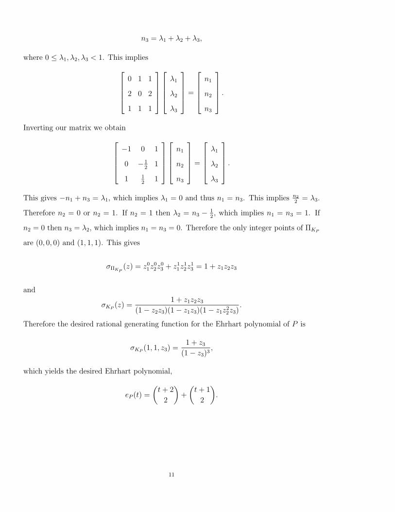
n3 = !1 + !2 + !3,

where 0 $ !1, !2, !3 < 1. This implies

/

0001

0 1 1

2 0 2

1 1 1

2

3334

/

0001

!1

!2

!3

2

3334=

/

0001

n1

n2

n3

2

3334.

Inverting our matrix we obtain

/

0001

(1 0 1

0 (12 1

1 12 1

2

3334

/

0001

n1

n2

n3

2

3334=

/

0001

!1

!2

!3

2

3334.

This gives (n1 + n3 = !1, which implies !1 = 0 and thus n1 = n3. This implies n22 = !3.

Therefore n2 = 0 or n2 = 1. If n2 = 1 then !2 = n3 ( 12 , which implies n1 = n3 = 1. If

n2 = 0 then n3 = !2, which implies n1 = n3 = 0. Therefore the only integer points of $KP

are (0, 0, 0) and (1, 1, 1). This gives

"!KP(z) = z0

1z02z

03 + z1

1z12z

13 = 1 + z1z2z3

and

"KP (z) =1 + z1z2z3

(1( z2z3)(1( z1z3)(1( z1z22z3)

.

Therefore the desired rational generating function for the Ehrhart polynomial of P is

"KP (1, 1, z3) =1 + z3

(1( z3)3,

which yields the desired Ehrhart polynomial,

eP (t) =

!t + 2

2

"+

!t + 1

2

".

11

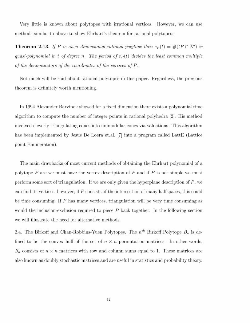
Very little is known about polytopes with irrational vertices. However, we can use

methods similar to above to show Ehrhart’s theorem for rational polytopes:

Theorem 2.13. If P is an n dimensional rational polytope then eP (t) = #(tP ' Zn) is

quasi-polynomial in t of degree n. The period of eP (t) divides the least common multiple

of the denominators of the coordinates of the vertices of P .

Not much will be said about rational polytopes in this paper. Regardless, the previous

theorem is definitely worth mentioning.

In 1994 Alexander Barvinok showed for a fixed dimension there exists a polynomial time

algorithm to compute the number of integer points in rational polyhedra [2]. His method

involved cleverly triangulating cones into unimodular cones via valuations. This algorithm

has been implemented by Jesus De Loera et.al. [7] into a program called LattE (Lattice

point Enumeration).

The main drawbacks of most current methods of obtaining the Ehrhart polynomial of a

polytope P are we must have the vertex description of P and if P is not simple we must

perform some sort of triangulation. If we are only given the hyperplane description of P , we

can find its vertices, however, if P consists of the intersection of many halfspaces, this could

be time consuming. If P has many vertices, triangulation will be very time consuming as

would the inclusion-exclusion required to piece P back together. In the following section

we will illustrate the need for alternative methods.

2.4. The Birko" and Chan-Robbins-Yuen Polytopes. The nth Birko" Polytope Bn is de-

fined to be the convex hull of the set of n # n permutation matrices. In other words,

Bn consists of n # n matrices with row and column sums equal to 1. These matrices are

also known as doubly stochastic matrices and are useful in statistics and probability theory.

12

For n " 2, the nth Chan-Robbins-Yuen Polytope (CYRn) is defined to be the convex

hull of the set of n# n permutation matrices, An, where if j " i + 2, then aij = 0. CYRn

has 2n&1 vertices and is#

n2

$dimensional. The fact that the row and column sums are 1,

provide the hyperplane description.

CYRn is a face of the nth Birko" polytope. While working on the Birko" polytope, Chan

and Robbins conjectured that the relative volume of CYRn is

RelVol(CYRn) =n&25

i=0

1

i + 1

!2i

i

",

the product of the first n ( 1 Catalan numbers. In the e"ort to prove this conjecture

Chan, Robbins and Yuen did extensive work on CYR. The conjecture was later proved by

Doron Zeilberger in 1998 [11]. The closed form for the volume of CYRn suggests a possible

recursion of the Ehrhart polynomials with respect to the dimensions. Such a recursion was

presented in [6].

Theorem 2.14. Let eCYRn(t) denote the Ehrhart polynomial for CYRn evaluated at t.

Then for every nonnegative integer t, the sequence

eCYR1(t), . . . , eCYRn(t), . . .

satisfies a linear recursion of degree p(t) with integer coe!cients, where p(t) is the number

of partitions of t.

Chan et.al. determined for t = 1, . . . , 12, there is no lower-degree recursion for the

sequence. However, it may be possible to find a lower-degree recursion for larger t. This

would be necessary as counting the number of partitions of t increases in di#culty as

t increases. One possible means finding a recursion of the Ehrhart polynomials is to

find a corresponding recursion between the rational generating functions for the sequence

13

eCYR1 , . . . , eCYRn , . . .. In the e"ort to find such recursions, we will explore the study of

partitions provided by Percy A. MacMahon.

14

3. MacMahon’s Partition Analysis

3.1. Introduction. In the early 1900s, Percy A. MacMahon developed the ! Operator

as a tool for enumerating partitions via their corresponding diophantine relations. In this

chapter, we will give an introduction to MacMahon’s techniques provided in his now classic

Combinatory Analysis [9].

3.2. Definition of !! and Identities. Define a partition of a positive integer t to be a list

of positive integers (a1, . . . , ak) arranged in descending order whose sum is t. The order of

a partition gives rise to a system of diophantine relations; a1 " a2 " a3 " . . . " ak, which

can be altered to produce various forms of partitions. For example, we can have partitions

of at most k parts, partitions into odd parts, partitions into distinct parts, etc.

For example the following generating function gives the number N(t) of ways three

nonnegative integers can sum to a positive integer t without taking into account the afore-

mentioned ordering, a1 " a2 " a3 " 0.

%

t!0

N(t)xt =%

ai!0

xa1+a2+a3 =%

a1!0

xa1%

a2!0

xa2%

a3!0

xa3 =1

(1( x)3.

Notice that the previous diophantine relations are equivalent to the following:

a1 ( a2 " 0

a2 ( a3 " 0

a3 " 0.

Considering this system, introduce a new variable for each inequality to obtain

%

ai!0

!a1&a21 !a2&a3

2 !a33 xa1+a2+a3 .

15

Now if we expand this series, eliminate all terms with negative powers, and set !1 = !2 =

!3 = 1, then we will obtain the generating function for partitions into at most 3 parts.

This is precisely what the operator !! does.

Definition 3.1. For a multiple Laurent series,

$%

!1,...!k=&$A!1,...!k

!!11 . . . !!k

k ,

define the operator !! by:

!!$%

!1,...!k=&$A!1,...!k

!!11 . . . !!k

k :=$%

!1,...!k=0

A!1,...!k.

Three of the many identities presented in [9] are:

Id 3.2.

!!1

(1( !x)(1( y")

=1

(1( x)(1( xy)

Id 3.3.

!!1

(1( !x)(1( y"2 )

=1

(1( x)(1( x2y)

Id 3.4.

!!1

(1( !2x)(1( y")

=1 + xy

(1( x)(1( xy2)

MacMahon leaves the verification of many of his identities to the reader. Therefore we

will now present them.

Proof. For Id 3.2, consider the crude generating function:

1

(1( !x)(1( y")

=%

ai!0

!a1&a2xa1ya2 .

If a2 > a1, then ! will have a negative power. To prevent this from happening, let

a1 ( a2 = b, force the restriction, b " 0 and make the appropriate substitutions into the

crude generating function to obtain

16

%

a2,b!0

!bxa2+bya2 =%

a2,b!0

(!x)b(xy)a2 =1

(1( !x)(1( xy).

In doing so, we have removed the possibilities for ! to have a negative power. Now if we

set ! = 1, we have the desired identity.

For Id 3.3, we similarly let a1 ( 2a2 = b, restrict b " 0 and make the appropriate

substitutions into%

ai!0

!a1&2a2xa1ya2 =1

(1( !x)(1( y"2 )

.

For Id 3.4, consider the following sum split into two parts:

%

ai!0

!2a1&a2xa1ya2 =%

a1!0a2=2k1+1

k1!0

!2a1&a2xa1ya2 +%

a1!0a2=2k1k1!0

!2a1&a2xa1ya2 .

Eliminate the terms in which ! has negative powers in the odd part by letting 2a1 =

2k2 + a2 = 2k1 + 2k2 + 2 for k2 " 0. Then a1 = k1 + k2 + 1, and

%

a1!0a2=2k1+1

k1!0

!2a1&a2xa1ya2 =%

ki!0

!2k2+1xk1+k2+1y2k1 = !xy%

ki!0

!2k2xk1+k2y2k1 .

Eliminate the terms in which ! has negative powers in the even part by letting 2a1 =

2k2 + a2 = 2k1 + 2k2 for k2 " 0. Then a1 = k1 + k2, and

%

a1!0a2=2k1k1!0

!2a1&a2xa1ya2 =%

ki!0

!2k2xk1+k2y2k1 .

Therefore,

%

ai!0

!2a1&a2xa1ya2 = !xy%

ki!0

!2k2xk1+k2y2k1 +%

ki!0

!2k2xk1+k2y2k1

17

= (1 + !xy)%

ki!0

!2k2xk1+k2y2k1

Setting ! = 1 we have Id 3.4. !

Returning to the example, regroup the variables of our generating function to obtain

%

ai!0

!a1&a21 !a2&a3

2 !a33 xa1+a2+a3 =

%

ai!0

(!1x)a1

!!2

!1x

"a2!

!3

!2x

"a3

,

which leads to the following crude generating function:

%

ai!0

(!1x)a1

!!2

!1x

"a2!

!3

!2x

"a3

=1

(1( !1x)&1( "2

"1x' &

1( "3"2

x' .

This equality allows us to conclude:

%

a1!a2!a3!0

xa1+a2+a3 = !!1

(1( !1x)(1( "2"1

x)(1( "3"2

x).

Now apply Id 3.2 to obtain

!"1!

1

(1( !1x)(1( "2"1

x)(1( "3"2

x)=

1

(1( x)(1( !2x2)(1( "3"2

x)

!"2!

1

(1( x)(1( !2x2)(1( "3"2

x)=

1

(1( x)(1( x2)(1( !3x3).

Now since there are no terms in which !3 has a negative power we have

!"3!

1

(1( x)(1( x2)(1( !3x3)=

1

(1( x)(1( x2)(1( x3).

Thus, the rational generation function for the number of ways to partition a positive

integer t into at most 3 parts is:

!!1

(1( !1x)(1( "2"1

x)(1( "3"2

x)=

1

(1( x)(1( x2)(1( x3).

18

Similarly it can be shown in general that the rational generating function for a positive

integer t into k parts is:

!!1

(1( !1x)(1( "2"1

x) . . . (1( "k"k!1

x)=

1

(1( x)(1( x2) . . . (1( xk).

3.3. Definition of != and Identities.

Definition 3.5. For a multiple Laurent series,

$%

!1,...!k=&$A!1,...!k

!!11 . . . !!k

k ,

define the operator != by:

!=

$%

!1,...!k=&$A!1,...!k

!!11 . . . !!k

k := A0, . . . , A0.

As with !!, MacMahon presents some identities for !=, two of which are:

Id 3.6.

!=1

(1( !x)#1( y

"

$ =1

(1( xy).

Id 3.7.

!=1

(1( !x)#1( y

"

$ #1( z

"

$ =1

(1( xy)(1( xz)

These lead to more general results:

Id 3.8.

!=1

(1( A1!)(1( A2!) · · · (1( An!)#1( y

"

$ =1

(1( A1y)(1( A2y) · · · (1( Any).

Id 3.9.

!=1

(1( A!)#1( y1

"

$ #1( y1

"

$· · ·

#1( yn

"

$ =1

(1( Ay1)(1( Ay2) · · · (1( Ayn)

19

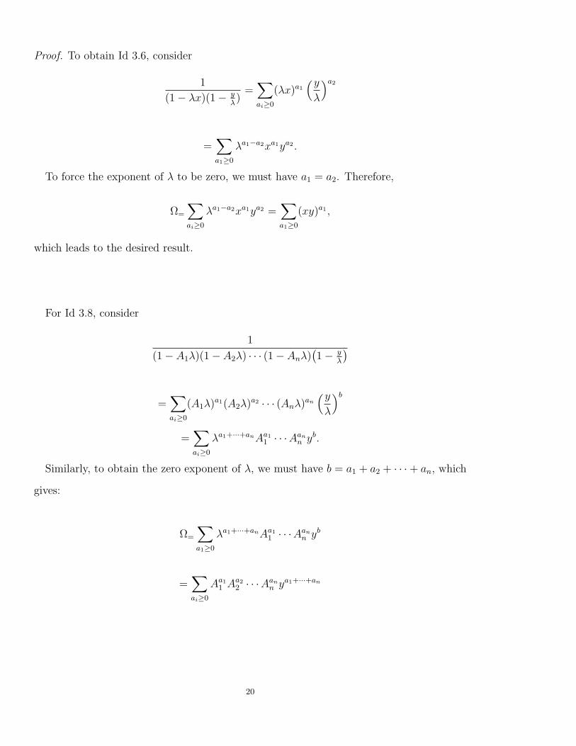
Proof. To obtain Id 3.6, consider

1

(1( !x)(1( y")

=%

ai!0

(!x)a1

&y

!

'a2

=%

a1!0

!a1&a2xa1ya2 .

To force the exponent of ! to be zero, we must have a1 = a2. Therefore,

!=

%

ai!0

!a1&a2xa1ya2 =%

a1!0

(xy)a1 ,

which leads to the desired result.

For Id 3.8, consider

1

(1( A1!)(1( A2!) · · · (1( An!)#1( y

"

$

=%

ai!0

(A1!)a1(A2!)a2 · · · (An!)an

&y

!

'b

=%

ai!0

!a1+···+anAa11 · · ·Aan

n yb.

Similarly, to obtain the zero exponent of !, we must have b = a1 + a2 + · · · + an, which

gives:

!=

%

a1!0

!a1+···+anAa11 · · ·Aan

n yb

=%

ai!0

Aa11 Aa2

2 · · ·Aann ya1+···+an

20

=%

ai!0

(A1y)a1(A2y)a2 · · · (Any)an .

Finally to obtain Id 3.9 we have:

1

(1( A!)#1( y1

"

$ #1( y1

"

$· · ·

#1( yn

"

$

=%

b,ai!0

(A!)b&y1

!

'a1&y2

!

'a2

· · ·&yn

!

'an

=%

b,ai!0

Ab!b&a1&···&anya11 · · · ya2

2 ,

and b( a1 ( · · ·( an = 0 if and only if b = a1 + · · · + an, therefore,

!=

%

ai!0

Ab!b&a1&···&anya11 · · · ya2

2

=%

ai!0

Aa1+···+anya11 · · · yan

n

=%

ai!0

(Ay1)a1(Ay2)

a2 · · · (Ayn)an .

!

In this paper we make use of two packages developed to do Omega calculus on com-

puter algebra systems. Andrews Et. Al. developed an package for Mathematica called the

Omega package [1] and and Xin developed a package for Maple called the Ell package [12].

3.4. Formal vs. Analytic. One question involving these crude generating functions is, are

we dealing with analytic or formal Laurent series? MacMahon was not explicit on this

matter, however Andrews et. al. [1] provide an argument as to why we should restrict

21

ourselves to the analytic. As rational functions we have

%

t!0

!txt +%

t<0

!txt = 0

and thus

(!!%

t<0

!txt = !!%

t!0

!txt =%

t!0

xt =1

1( x.

However,

!!%

t!0

!txt =%

t!0

xt =1

1( x

and

(!!%

t<0

!txt = 0.

Therefore, considering formal series does not permit the Omega operators to be well-

defined. As a result, we must restrict MacMahon’s Omega Calculus to the rational func-

tions corresponding to converging Laurent series.

22

4. Partition Analysis and Polytopes

4.1. Introduction. Applying MacMahon’s Partition analysis to polytopes can be done in

a manner quite similar to the process of coning over a polytope. As with the coning

process we obtain some sort of an embedding of the polytope’s generating function into

a grander sort of generating function, in this case the crude generating functions. Then

we apply the appropriate Omega operator to recover the desired generating function. The

main advantages are that we no longer require the use of triangulation and if we are only

given the hyperplane description of a polytope, we do not have to convert to the vertex

description.

4.2. The General Idea. Consider a rational polytope’s hyperplane description, P := {x !

Rn|Ax " b}. Note if P is rational we can assume all the entries of A and b are integral.

For each defining halfspace aix( tbi " 0 embed !(aix&tbi)i into a crude generating function.

Since it only makes sense to consider positive dilations, we have the constraint t " 0.

Embed yt in the crude generating function as well to obtain

F (!, y) =%

xi,t!0

!(a1x&tb1)1 !(a2x&tb2)

2 · · ·!(amx&tbm)m yt.

Then the corresponding crude rational generating function is

1

(1( !a111 !a21

2 · · ·!am1m ) · · · (1( !a1n

1 !a2n2 · · ·!amn

m )&1( y

"b11 "

b22 ···"bm

m

' ,

where aij is the (ij)th entry of A.

Theorem 4.1. If P := {x ! Rn|Ax " b} is an integral polytope with Ehrhart polynomial

eP (t) and

F (!, y) =1

(1( !a111 !a21

2 · · ·!am1m ) · · · (1( !a1n

1 !a2n2 · · ·!amn

m )&1( y

"b11 "

b22 ···"bm

m

'

23

where aij is the (ij)th entry of A then

%

t!0

eP (t)yt = !!F (!, y).

Proof. If P := {x ! Rn|Ax " b} then #(tP ' Zn) = #({x ! Rn|Ax " tb} ' Zn). A point

x ! Rn is a solution for a halfspace inequality aix " tbi if and only if aix( tbi " 0.

Let

F )(!, y, z) :=

1

(1( z1!a111 !a21

2 · · ·!am1m ) · · · (1( zn!

a1n1 !a2n

2 · · ·!amnm )

&1( y

"b11 "

b22 ···"bm

m

'

Note F )(!, y, 1) = F (!, y) and

F )(!, y, z) =

%

xi,t!0

(z1!a111 !a21

2 · · ·!am1m )x1 · · · (zn!

a1n1 !a2n

2 · · ·!amnm )xn

!y

!b11 !b2

2 · · ·!bmm

"t

=%

xi,t!0

!(a1x&tb1)1 !(a2x&tb2)

2 · · ·!(amx&tbm)m zx1

1 zx22 · · · zxn

n yt.

Then

!!F )(!, y, z) =

!!%

xi,t!0

!(a1x&tb1)1 !(a2x&tb2)

2 · · ·!(amx&tbm)m zx1

1 zx22 · · · zxn

n yt

=%

aix&bi!0xi,t!0

zx11 zx2

2 · · · zxnn yt

=%

t!0x'(t·P(Zn)

zx11 zx2

2 · · · zxnn yt.

Therefore

!!F (!, y) = !!F )(!, y, 1) =%

t!0

ep(t)yt.

24

!

Similarly we have

Theorem 4.2. If P{x ! Rn|Ax " b} is a rational polytope with Ehrhart quasi-polynomial

Qp(t) and

F (!, y) =1

(1( !a111 !a21

2 · · ·!am1m ) · · · (1( !a1n

1 !a2n2 · · ·!amn

m )&1( y

"b11 "

b22 ···"bm

m

'

where aij is the (ij)th entry of A then

%

t!0

QP (t)yt = !!F (!, y).

Let t be a positive integer and recall the polytope:

P := {(x1, x2) ! R2 | x2 + 2x1 " 2, 2 " x2, and 1 " x1},

then the number of integer points contained in t · P is equivalent to the number of integer

solutions of the following system:

x2 + 2x1 ( 2t " 0

2t( x2 " 0

t( x1 " 0

t " 0.

Encode this system into a crude generating function to obtain

%

xi,t!0

!x2+2x1&2t1 !2t&x2

2 !t&x13 yt,

which corresponds to the following crude rational generating function:

1

(1( "21

"3)(1( "1

"2)(1( "2

2"3

"21

y).

25

To find the desired rational generating function, we use the three identities provided

above, and we have

!"3!

1

(1( "21

"3)(1( "1

"2)(1( "2

2"3

"21

y)=

1

(1( "1"2

)(1( "22

"21y)(1( !2

2y)

!"1!

1

(1( "1"2

)(1( "22

"21y)(1( !2

2y)=

1

(1( y)(1( !22y)(1( 1

"2)

!"2!

1

(1( y)(1( !22y)(1( 1

"2)

=1 + y

(1( y)3.

Therefore we can conclude:

!!1

(1( "21

"3)(1( "1

"2)(1( "2

2"3

"21

y)=

1 + y

(1( y)3.

This is the same rational generation function we obtained above via conventional methods.

For another example let

P :=

6x ! R3

7777Ax $ b

8,

where

A =

/

00000001

1 1 1

1 (1 (1

(1 1 (1

(1 (1 1

2

33333334

and b =

/

00000001

2

0

0

0

2

33333334

.

26

Then the number of lattice points in t ·P is equivalent to the number of integer solutions

to the system

2t( x1 ( x2 ( x3 " 0

(x1 + x2 + x3 " 0

x1 ( x2 + x3 " 0

x1 + x2 ( x3 " 0

t " 0.

Encoding this system into a crude generating function we have

%

x1!0

!2t&x1&x1&x31 !&x1+x2+x3

2 !x1&x2+x33 !x1+x2&x3

4 yt =1

(1( "3"4"1"2

)(1( "2"4"1"3

)(1( "3"2"1"4

)(1( !21y)

.

Using the Omega package [1] to apply !! we obtain:

!"1!

1

(1( "3"4"1"2

)(1( "2"4"1"3

)(1( "3"2"1"4

)(1( !21y)

=1 + y!2

2 + y!23 + y"2"3

"4+ y"2"4

"3+ y"4"3

"2+ y2!2!3!4 + 4!2

4

(1( y)(1( y"22"2

3

"24

)(1( y"22"2

4

"23

)(1( y"24"2

3

"22

)

!"2!

1 + y!22 + y!2

3 + y"2"3

"4+ y"2"4

"3+ y"4"3

"2+ y2!2!3!4 + 4!2

4

(1( y)(1( y"22"2

3

"24

)(1( y"22"2

4

"23

)(1( y"24"2

3

"22

)

=1( y3!3!4 + y(1 + "3

"4+ "4

"3) + y2((!2

3 ( !3!4 ( !24)

(1( y)(1( y!23)(1(

y"23

"24)(1( y!2

4)(1(y"2

4

"23)

!"3!

1( y3!3!4 + y(1 + "3"4

+ "4"3

) + y2((!23 ( !3!4 ( !2

4)

(1( y)(1( y!23)(1(

y"23

"24)(1( y!2

4)(1(y"2

4

"23)

=1 + y(1 + 1

"4) + y2

"4

(1( y)2(1( y"24)(1( y!2

4)

!"4!

1 + y(1 + 1"4

) + y2

"4

(1( y)2(1( y"24)(1( y!2

4)

=1 + y2

(1( y)4.

27

Therefore the rational generating function for the number of lattice points in t · P is

1 + y2

(1( y)4,

which gives rise to the desired Ehrhart polynomial

e(t) =

!t + 3

3

"+

!t + 1

3

".

4.3. Partition Analysis and CYR. CYRn consists of n# n matrices of the form

/

00000000001

x11 x12 0 0 · · ·

x21 x22 x23 0 · · ·...

......

. . .

xn&1,1 xn&1,2 xn&1,3 · · · xn&1,n

xn1 xn2 xn3 · · · xnn

2

33333333334

,

where the row and columns both sum to 1.

Since CYRn has 2n&1 vertices, triangulation will be very time consuming, however, the

fact that the row and columns of CYRn both sum to 1 provide us with the hyperplane

description. Therefore we can use partition analysis to find eCYRn(t).

For example, the number of lattice points in CYR3 is equivalent to the number of integer

solutions to the following system:

x11 + x12 = t

x21 + x22 + x23 = t

x31 + x32 + x33 = t

x11 + x21 + x31 = t

x12 + x22 + x32 = t

28

x23 + x33 = t.

Encoding this into a crude generating function we have

CYR3(!, y) =

1

(1( !1!4)(1( !1!5)(1( !2!4)(1( !2!5). . .

1

(1( !2!6)(1( !3!4)(1( !3!5)(1( !3!6)#1( y

"1···"6

$ .

Using the aforementioned identities for != we obtain:

!"1= CYR3(!, y) =

1&1( y

"2"3"5"6

' &1( y

"2"3"4"6

' . . .

1

(1( !2!4)(1( !2!5)(1( !2!6)(1( !3!4)(1( !3!5)(1( !3!6)

!"5= !"1

= CYR3(!, y) =

1

(1( y"3"6

)(1( y"2"6

)(1( y"2"3"4"6

). . .

1

(1( !2!4)(1( !2!6)(1( !3!4)(1( !3!6)

!"4= !"5

= !"1= CYR3(!) =

1

(1( y"3"6

)(1( y"2"6

)(1( y"3"6

)(1( y"2"6

)(1( !2!6)(1( !3!6)

!"3= !"4

= !"5= !"1

= CYR3(!, y) =

29

1

(1( y)2&1( y

"2"6

'2

(1( !2!6)

!"6= !"3

= !"4= !"5

= !"1= CYR3(!, y) =

1

(1( y)4.

Therefore

!=CYR3(!, y) =1

(1( y)4.

Also we can easily obtain

!=CYR2(!, y) =1

(1( y)2.

Using the Omega Package we obtain:

!=CYR4(!, y) =y + 1

(1( y)7,

!=CYR5(!, y) =4y2 + 5y + 1

(y ( 1)11.

Using the Ell package we obtain:

!=CYR6(!, y) =9y4 + 56y3 + 58y2 + 16y + 1

(1( y)16.

These rational functions give rise to the desired Ehrhart polynomials:

eCYR2(t) = t + 1

eCYR3(t) =

*

+ t + 3

3

,

-

eCYR4(t) =

*

+ t + 6

6

,

- +

*

+ t + 5

6

,

-

30

eCYR5(t) =

*

+ t + 10

10

,

- + 5

*

+ t + 9

10

,

- + 4

*

+ t + 8

10

,

-

eCYR6(t) =

*

+ t + 15

14

,

- + 16

*

+ t + 14

15

,

- + 58

*

+ t + 13

15

,

-

+56

*

+ t + 12

15

,

- + 9

*

+ t + 11

15

,

- .

31

5. On the Hunt for a New Algorithm

5.1. Introduction. The packages developed by Xin and Andrews et. al. have been very

helpful, however the author’s personal computer could not process the computations re-

quired to go beyond eCYR6 . This may be due to the fact that both packages require

simplifying sums of rational functions, which as Xin points out in [12] both Maple and

Mathematica have di#culties performing. Therefore it would be useful to find a more

e#cient algorithm by finding possible means of reducing the simplifications required and

merging them with the techniques used to develop the Omega and Ell packages. In this

chapter we describe possible avenues leading to such an algorithm.

5.2. Symmetric Functions. In this section, we present the possible beginnings of a more

algebraic algorithm to compute !=F (!, x, y), where

F (!, x, y) :=1

(1( x1!)(1( x2!) · · · (1( xn!)#1( y1

"

$ #1( y2

"

$· · ·

#1( ym

"

$ .

Let t be a positive integer. A composition of t is a sequence of integers, whose sum is t.

Let Ck,t be the set of all compositions of t into at most k parts. Then using terminology

provided in [10] define a weighting of Cn to be the function wt : Cn * C [[x]] defined by

wt c := xa11 xa2

2 · · ·xann ,

where C [[x]] is the ring of formal power series in x over C and c = (a1, . . . , an). Define

fCn,t(x) :=%

c'Cn,t

wt c.

Note for fixed n%

t!0

fCn,t(x)yt = !=F )(!, y, x),

where

32

F )(!, y, x) :=%

ai,t!0

!a1+···+an&txa11 xa2

2 · · ·xann yt

=1

(1( x1!)(1( x2!) · · · (1( xn!)#1( y

"

$ .

Therefore%

t!0

fCn,t(x)yt =1

(1( x1y)(1( x2y) · · · (1( xny).

Theorem 5.1. If

F (!, x, y) :=19n

i=1(1( xi!)9m

i=1

#1( yi

"

$

then

!=F (!, x, y) =

%

t!0

fCn+m,2t(x, y)zt ( !"2= !"1

!

1"19n

i=1(1( !1!2xi)9m

i=1(1( !2yi)&1( z

"1"22

'

(!"2= !"3

!

1"39m

i=1(1( !3!2yi)9n

i=1(1( !2xi)&1( z

"3"22

' .

evaluated at z = 1.

Proof. Let

F (!, x, y) :=19n

i=1(1( xi!)9m

i=1

#1( yi

"

$ .

Then

F (!, x, y) =%

ai,bi!0

(x1!)a1(x2!)a2 · · · (xn!)an

&y1

!

'b1 &y2

!

'b2· · ·

&ym

!

'bm

=%

ai,bi!0

xa11 xa2

2 · · ·xann yb1

1 yb22 · · · ybm

m !a1+···+an&b1&···&bm .

33

Applying != to F (!, x, y) is equivalent to eliminating all terms except for those with

exponents satisfying the condition

n%

i=1

ai =m%

i=1

bi = t for some t ! Z!0.

Therefore

!=F (!, x, y) = F )(!, x, y, 1),

where

F )(!, x, y, z) =%

t!0

fCn,t(x)fCm,t(y)zt.

If c1 = (a1, ...an) ! Cn,t and c2 = (b1, . . . , bm) ! Cm,t then c1c2 := (a1, . . . , an, b1, . . . , bm) !

Cn+m,2t, however, fCn,t(x) · fCm,t(y) %= fCn+m,2t(x, y) because we can have a composition of

2t where the first n terms do not sum to t. Therefore we can conclude

%

t!0

fCn,t(x)fCm,t(y)zt =

%

t!0

fCn+m,2t(x, y)zt (%

t!0

:%

k>t

fCn,k(x)fCm,2t!k(y)

;zt

(%

t!0

:%

k<t

fCn,k(x)fCm,2t!k

(y)

;zt

=%

t!0

fCn+m,2t(x, y)zt (%

t!0

:%

k>t

fCn,k(x)fCm,2t!k

(y)

;zt

(%

t!0

:%

k>t

fCn,2t!k(x)fCm,k

(y)

;zt.

Notice%

t!0

:%

k>t

fCn,k(x)fCm,2t!k

(y)

;zt =

!"2= !"1

!

%

ai,bi!0t!0

xa11 · · ·xan

n yb11 · · · ybm

m zt!a1+···+an&t&11 !b1+···+bm+a1+···+an&2t

2

34

= !"2= !"1

!

1"19n

i=1(1( !1!2xi)9m

i=1(1( !2yi)&1( z

"1"22

' .

Similarly we have

%

t!0

:%

k>t

fCn,2t!k(x)fCm,k

(y)

;zt = !"2

= !"3!

1"39m

i=1(1( !3!2yi)9n

i=1(1( !2xi)&1( z

"3"22

' .

!

Notice that%

t!0

fCn+m,2t(x, y)zt =

=%

ai,bi!0t!0

xa11 · · ·xan

n yb11 · · · ybm

m zt!a1+···+an+b1+···+bm&2t

!=19n

i=1(1( xi!)9m

i=1(1( yi!)#1( z

"2

$ .

If we can find the rational generating function for

%

t!0

fCn+m,2t(x, y)zt

then we can apply the following theorem provided by G.N. Han [8] to produce a finalized

result:

Theorem 5.2. If n ! Z! and U(!) be a Laurent polynomial with degree less than n ( 1

then

!!U(!)9n

i=1(1( xi!)9m

i=1

#1( yi

"

$ =n%

i=1

xn&1i U

&1xi

'

(1( xi)9m

j=1(1( xiyj)9

j *=i(xi ( xj).

The formula holds even when the xi’s are not all distinct.

35

5.3. Switching Gears. One can argue that applying partition analysis to polytopes is a

generalization of MacMahon’s original intent in that every form of partition given by

Diophantine relations has a polyhedra interpretation. Therefore, it makes sense to switch

roles and apply Ehrhart theory to partition analysis. Making use of Theorem 2.4 we provide

alternate proofs for some of MacMahon’s identities, which we restate for convenience.

Id 5.3.

!!1

(1( !z1)(1( z2" )

=1

(1( z1)(1( z1z2)

Id 5.4.

!!1

(1( !z1)(1( z2"2 )

=1

(1( z1)(1( z21z2)

Id 5.5.

!!1

(1( !2z1)(1( z2" )

=1 + z1z2

(1( z1)(1( z1z22)

Proof. For Id 5.3 Let

K := {a1 ( a2 " 0|ai ! R+}.

Then one can easily show that K is a simple cone with (1, 1) and (1, 0) as generators.

Therefore by Theorem 2.4 we have

"K(z) ="!K (z)

(1( z(1,1))(1( z(1,0)),

where $K := {!1(1, 1) + !2(1, 0)|0 $ !1, !2 < 1}. Since the only lattice point in $K is

(0, 0) we have,

"K(z) =z01z

02

(1( z11z

12)(1( z1

1z02)

.

Thus we have the desired identity.

Similarly we can obtain Id 5.4 by considering the cone

K := {a1 ( 2a2 " 0|ai ! R+},

36

which has generators (1, 0) and (2, 1) with $K := {!1(1, 0)+!2(2, 1)|0 $ !1, !2 < 1}. Once

again $K ' Z = {(0, 0)} so we have

"K(z) =z01z

02

(1( z11z

02)(1( z2

1z12)

.

For Id 5.5 consider

K := {2a1 ( a2 " 0|ai ! R+},

which has generators (0, 1) and (1, 2) with $K := {!1(0, 1) + !2(1, 2)|0 $ !1, !2 < 1}. We

have $K ' Z = {(0, 0), (1, 1)} and thus

"K(z) =z01z

02 + z1

1z12

(1( z01z

12)(1( z1

1z22)

.

!

5.4. Five Guidelines for !!. Corteel, Lee and Savage [5] have developed five guidelines that

provide a simplification of MacMahon’s partition analysis for integral, linear, homogenous

systems of inequalities. We will discuss these guidelines and then expand on them to in-

clude linear systems of equalities. To do so we will first cover the terminology presented

in [5].

A constraint c is a linear inequality of the form,

a0 +n%

i=1

aixi " 0,

The negation of constraint c denoted by ¬c is the linear inequality

(a0 (n%

i=1

aixi > 0.

Let C denote a set of constraints, and Cxi+xi+axj denote the set of constraints formed

by substituting the variable xi with xi + axj in all constraints contained in C. SC denotes

37

the set of integer points satisfying all constraints in C, and

FC(!) =%

x'SC

!x11 !x2

2 · · ·!xnn

denotes the full generating function for SC . A constraint c is said to be implied by a set

of constraints C if SC,{¬c} = !. As we are often only interested in nonnegative solutions,

we will assume that any set of constraints on variables xi contain the constraints xi " 0

for all i regardless of equality conditions. Before we state the five guidelines, we will first

present a slightly more generalized version of a lemma provided in [5].

Lemma 5.6. Let C be a set of linear homogenous inequalities and suppose the constraint,

xi ( #(x) " 0 is implied by C, where

#(x) :=%

j *=i

bjxj

and bj ! Z for all j. Let C " = Cxi+xi+#(x). Then,

! = (!1, !2, . . . ,!n) ! SC

if and only if

!" = (!1, . . . ,!i&1, !i ( #(!), !i+1, . . . ,!n) ! SC" .

Proof. Let

c(x) := a0 +n%

k=1

akxk

and

c"(x) := a0 +i&1%

k=1

akxk + ai[xi + #(x)] +n%

k=i+1

akxk.

Suppose C is a set of linear homogenous equalities and C contains the constraint c(x) " 0.

Then C " contains the constraint c"(x) " 0, where C " = Cxi+xi+#(x).

38

If !" = (!1, . . . ,!i&1, !i ( #(!), !i+1, . . . ,!n) then

c"(!") = a0 +i&1%

k=1

ak!k + ai [(!i ( #(!)) + #(!)] +n%

k=i+1

ak!k

= a0 +n%

k=1

ak!k = c(!).

Therefore ! = (!1, !2, . . . ,!n) satisfies c ! C if and only if !" = (!1, . . . ,!i&1, !i (

#(!), !i+1, . . . ,!n) satisfies c" ! C ". Now we need to verify nonnegativity conditions.

If the constraint, xi ( #(x) " 0 is implied by C, where

#(x) :=%

j *=i

bjxj

and bj ! Z for all j then ! ! SC implies !i ( #(!) " 0 and !j " 0 for all j. Therefore

!" ! SC" . The constraint, xi " 0 ! C implies the constraint, xi +#(x) " 0 ! C ". Therefore,

!" ! SC" implies [!i ( #(!)] + #(!) " 0, which implies !i " 0. Therefore, ! ! SC . !

The Five Guidelines [5]

Theorem 5.7. Let t be a fixed, nonnegative integer. If C = {x " t}, then

FC(!) =!t

(1( !).

This follows from geometric series since

FC(!) =%

s!0

!t+s.

Theorem 5.8. If C1 is a set of constraints on variables x1, . . . , xj and C2 is a set of

constraints on variables xj+1, . . . , xn, then

FC1,C2(!) = FC1(!1, . . . ,!j)FC2(!j+1, . . . ,!n).

39

This is true because (x1, . . . , xn, y1, . . . ym) ! SC1,C2 if and only if (x1, . . . , xn) ! SC1 and

(y1, . . . , ym) ! SC1 .

Theorem 5.9. Let C be a set of linear homogenous inequalities of variables x1, . . . , xn and

with the constraints xi " 0. Suppose xi ( #(x) " 0 is implied by C, where

#(x) :=%

j *=i

bjxj

and bj ! Z for all j. If C " = Cxi+xi+#(x) then,

FC(!) = FC"(!; !j + !j!bj

i , ,j %= i).

Proof. Lemma 5.6 gives, (!1, !2, . . . ,!n) ! SC" if and only if (!1, . . . ,!i&1, !i+#(!), !i+1, . . . ,!n) !

SC . Therefore we have:

FC"(!; !j + !j!bj

i , ,j %= i)

=%

x'SC"

(!1!b1i )x1 · · · (!i&1!

bi!1

i )xi!1!i(!i+1!bi+1

i )xi+1 · · · (!n!bni )xn

=%

x'SC"

!x11 · · ·!xi!1

i&1 !xi+#(x)i !xi+1

i+1 · · ·!xnn

=%

x'SC

!x11 !x2

2 · · ·!xii · · ·!xn

n = FC(!).

!

Theorem 5.10. Let c be a constraint with the same variables as the ones occurring in the

set C. Then

FC(!n) = FC,{c}(!n) + FC,{¬c}(!n).

This holds because (x1, . . . , xn) ! SC satisfies either c or ¬c but not both.

Theorem 5.11. Let c ! C. Then

FC(!n) = FC\{c}(!n)( F{C\{c}},{¬c}(!n).

40

This holds because {C \ {c}} - {c} = C and by the previous guideline we have

FC\{c}(!) = F{C\{c}},{c}(!) + F{C\{c}},{¬c}(!).

5.5. Guidelines for !=. We are now going to consider integral systems of homogeneous

linear equations. Let c be a constraint of the form

a0 +n%

k=1

akxk = 0.

Define the negation of c to be

¬c :

<¬c1 : a0 +

=nk=1 akxk " 1

¬c2 : ( a0 (=n

k=1 akxk " 1.

Then we say a constraint c is implied by C if

SC,{¬c1} = SC,{¬c2} = !.

Lemma 5.12. Suppose the constraint, xi ( #(x) = 0 is implied by C, where

#(x) :=%

j *=i

bjxj

and bj ! Z for all j.

Let C " = Cxi+xi+#(x). Then,

! = (!1, !2, . . . ,!n) ! SC

if and only if

!" = (!1, . . . ,!i&1, !i ( #(!), !i+1, . . . ,!n) ! SC" .

41

Proof. The proof of this lemma is identical to the analogous lemma for inequalities except

of the verification of nonnegativity. If the constraint, xi(#(x) = 0 is implied by C, where

#(x) :=%

j *=i

bjxj

and bj ! Z for all j then ! ! SC implies !i ( #(!) = 0 and !i " 0 for all i. Therefore

!" ! SC" . The constraint, xi " 0 ! C implies the constraint, xi + #(x) " 0 ! C ".

Therefore, !" ! SC" implies !i ( #(!) " 0 and !i + #(!) " 0, which implies !i " 0.

Therefore, ! ! SC . !

Theorem 5.13. Let C be a set of linear homogenous equalities of variables x1, . . . , xn and

with the constraints xi " 0. Suppose xi ( #(x) = 0 is implied by C, where

#(x) :=%

j *=i

bjxj

and bj ! Z for all j. If C " = Cxi+xi+#(x) then,

FC(!) = FC"(!; !j + !j!bj

i , ,j %= i).

Once again, using Lemma 5.12 instead of Lemma 5.6, the proof of this theorem is

identical to the analogous theorem for inequalities.

42

6. Future Work

This paper is the mere beginnings of a much larger project. In this paper we have

presented possible leads for combining Ehrhart theory with partition analysis that have

yet reach to their potential. It is the intent of the author to explore these routes in hopes to

find a more computational friendly algorithm for Omega calculus, implement the algorithm

into a computer algebra system and apply these methods to high-dimensional polytopes

such as CYRn and the Birko" polytope.

43

References

[1] G.E. Andrews, P. Paule, and A. Riese, Macmahon’s Partition Analysis: The Omega Package. Euro-

pean Journal of Combinatorics, October 2001, vol 22, iss. 7, pp. 887-904(18) Academic Press, London.

[2] Alexander Barvinok, Apolynomial time algorithm for counting integral points in polyhedra when the

dimension is fixed. Mathematics of Operations Research (19), 1994, 769-779.

[3] Matthias Beck and Sinai Robbins,Computing the Continuous Discretely, Springer, to appear.

[4] Dimitris Bertsimas and John N. Tsitsiklis, Introduction to Linear Optimization, Athena Scientific,

Belmont, MA, 1997.

[5] Sylvie Cortell, Sunyoung Lee, and Carla D. Savage, Five Guidelines for Partition Analysis with Appli-

cations to Lecture Hall-type Theorems. Integers, to appear (Special volume of the Proceedings of the

Intergers Conference 2005 in honor of Ron Graham). See http://www.csc.ncsu.edu/faculty/savage/.

[6] Clara S. Chan, David P. Robbins, and David S. Yuen, On the Volume of a Certain Polytope. Experi-

mental Mathematics, 1999, vol 9, iss. 1, pp. 91-99.

[7] De Loera http://www.math.ucdavis.edu/.latte/

[8] G.N. Han A general algorithm for the MacMahon Omega operator. Ann. of Comb. (7), 2003, 467-480.

[9] P. A. Macmahon, Combinatory Analysis, 2 Vols. Cambridge University Press, Cambridge, 1915-1916.

(Reprinted: Chelsea Pub. Co., NY, 1984)

[10] Bruce E. Sagan, The Symmetric Group: Representations, Combinatorial Algorithms, and Symmetric

Functions, Second Edition. Springer-Verlag, New York 2001.

[11] Doron Zeilberger, Proof of a conjecture of Chan, Robbins and Yuen. ETNA, Elec. Trans, of Numerical

Analysis (9), 1999, 147-148.

[12] Guouce Xin, A Fast Algorithm for MacMahon’s Partition Analysis. Elect. Journal of Comb. (11),

2004, R58, 20pp.

44