A Theory of Name Resolution

Pierre Neron1, Andrew Tolmach2, Eelco Visser1, and Guido Wachsmuth1

1) Delft University of Technology, The Netherlands,{p.j.m.neron, e.visser, g.wachsmuth}@tudelft.nl,

2) Portland State University, Portland, OR, USAtolmach@pdx.edu

Abstract. We describe a language-independent theory for name bindingand resolution, suitable for programming languages with complex scop-ing rules including both lexical scoping and modules. We formulate nameresolution as a two-stage problem. First a language-independent scopegraph is constructed using language-specific rules from an abstract syn-tax tree. Then references in the scope graph are resolved to correspond-ing declarations using a language-independent resolution process. Weintroduce a resolution calculus as a concise, declarative, and language-independent specification of name resolution. We develop a resolutionalgorithm that is sound and complete with respect to the calculus. Basedon the resolution calculus we develop language-independent definitionsof α-equivalence and rename refactoring. We illustrate the approach us-ing a small example language with modules. In addition, we show howour approach provides a model for a range of name binding patterns inexisting languages.

1 Introduction

Naming is a pervasive concern in the design and implementation of programminglanguages. Names identify declarations of program entities (variables, functions,types, modules, etc.) and allow these entities to be referenced from other partsof the program. Name resolution associates each reference to its intended decla-ration(s), according to the semantics of the language. Name resolution underliesmost operations on languages and programs, including static checking, trans-lation, mechanized description of semantics, and provision of editor services inIDEs. Resolution is often complicated, because it cuts across the local inductivestructure of programs (as described by an abstract syntax tree). For example,the name introduced by a let node in an ML AST may be referenced by anarbitrarily distant child node. Languages with explicit name spaces lead to fur-ther complexity; for example, resolving a qualified reference in Java requires firstresolving the class or package name to a context, and then resolving the membername within that context. But despite this diversity, it is intuitively clear thatthe basic concepts of resolution reappear in similar form across a broad range oflexically-scoped languages.

In practice, the name resolution rules of real programming languages areusually described using ad hoc and informal mechanisms. Even when a lan-guage is formalized, its resolution rules are typically encoded as part of static

Pierre Neron, Andrew P. Tolmach, Eelco Visser, Guido Wachsmuth. A Theory ofName Resolution. In Jan Vitek (editor), Programming Languages and Systems - 24thEuropean Symposium on Programming, ESOP 2015, Held as Part of the EuropeanJoint Conferences on Theory and Practice of Software, ETAPS 2015, London, UK,April 11-18, 2015, Proceedings. Lecture Notes in Computer Science, Springer, April2015.

2

and dynamic judgments tailored to the particular language, rather than beingpresented separately using a uniform mechanism. This lack of modularity in lan-guage description is mirrored in the implementation of language tools, where theresolution rules are often encoded multiple times to serve different purposes, e.g.,as the manipulation of a symbol table in a compiler, a use-to-definition displayin an IDE, or a substitution function in a mechanized soundness proof. This rep-etition results in duplication of effort and risks inconsistencies. To see how muchbetter this situation might be, we need only contrast it with the realm of syntaxdefinition, where context-free grammars provide a well-established declarativeformalism that underpins a wide variety of useful tools.

Formalizing resolution. This paper describes a formalism that we believe canhelp play a similar role for name resolution in lexically-scoped languages. It con-sists of a scope graph, which represents the naming structure of a program, anda resolution calculus, which describes how to resolve references to declarationswithin a scope graph. The scope graph abstracts away from the details of a pro-gram AST, leaving just the information relevant to name resolution. Its nodesinclude name references, declarations, and “scopes,” which (in a slight abuse ofconventional terminology) we use to mean minimal program regions that behaveuniformly with respect to name resolution. Edges in the scope graph associatereferences to scopes, declarations to scopes, or scopes to “parent” scopes (corre-sponding to lexical nesting in the original program AST). The resolution calculusspecifies how to construct a path through the graph from a reference to a decla-ration, which corresponds to a possible resolution of the reference. Hiding of onedefinition by a “closer” definition is modeled by providing an ordering on reso-lution paths. Ambiguous references correspond naturally to multiple resolutionpaths starting from the same reference node; unresolved references correspondto the absence of resolution paths. To describe programs involving explicit namespaces, the scope graph also supports giving names to scopes, and can include“import” edges to make the contents of a named scope visible inside anotherscope. The calculus supports complex import patterns including transitive andcyclic import of scopes.

This language-independent formalism gives us clear, abstract definitions forconcepts such as scope, resolution, hiding, and import. We build on these con-cepts to define generic notions of α-equivalence and valid renaming. We also givea practical algorithm for computing conventional static environments mappingbound identifiers to the AST locations of the corresponding declarations, whichcan be used to implement a deterministic, terminating resolution function thatis consistent with the calculus. We expect that the formalism can be used asthe basis for other language-independent tools. In particular, any tool that relieson use-to-definition information, such as an IDE offering code completion foridentifiers, or a live variable analysis in a compiler, should be specifiable usingscope graphs.

On the other hand, the construction of a scope graph from a given program isa language-dependent process. For any given language, the construction can bespecified by a conventional syntax-directed definition over the language gram-

3

mar; we illustrate this approach for a small language in this paper. We wouldalso like a more generic binding specification language which could be used todescribe how to construct the scope graph for an arbitrary object language. Wedo not present such a language in this paper. However, the work described herewas inspired in part by our previous work on NaBL [16], a DSL that provideshigh-level, non-algorithmic descriptions of name binding and scoping rules suit-able for use by a (relatively) naive language designer. The NaBL implementationintegrated into the Spoofax Language Workbench [14] automatically generatesan incremental name resolution algorithm that supports services such as codecompletion and static analysis. However, the NaBL language itself is definedlargely by example and lacks a high-level semantic description; one might saythat it works well in practice, but not in theory. Because they are language-independent, scope graphs can be used to give a formal semantics for NaBLspecifications, although we defer detailed exploration of this connection to fur-ther work.

Relationship to Related Work. The study of name binding has received a greatdeal of attention, focused in particular on two topics. The first is how to represent(already resolved) programs in a way that makes the binding structure explicitand supports convenient program manipulation “modulo α-equivalence” [7, 20, 3,10, 4]. Compared to this work, our system is novel in several significant respects.(i) Our representation of program binding structure is independent of the under-lying language grammar and program AST, with the benefits described above.(ii) We support representation of ill-formed programs, in particular, programswith ambiguous or undefined references; such programs are the normal case inIDEs and other front-end tools. (iii) We support description of binding in lan-guages with explicit name spaces, such as modules or OO classes, which arecommon in practice.

A second well-studied topic is binding specification languages, which are usu-ally enriched grammar descriptions that permit simultaneous specification oflanguage syntax and binding structure [22, 8, 13, 23, 25]. This work is essentiallycomplementary to the design we present here.

Specific contributions.

– Scope Graph and Resolution Calculus: We introduce a language-independentframework to capture the relations among references, declarations, scopes,and imports in a program. We give a declarative specification of the res-olution of references to declarations by means of a calculus that definesresolution paths in a scope graph (Section 2).

– Variants: We illustrate the modularity of our core framework design by de-scribing several variants that support more complex binding schemes (Sec-tion 2.5).

– Coverage: We show that the framework covers interesting name binding pat-terns in existing languages, including various flavors of let bindings, qualifiednames, and inheritance in Java (Section 3).

4

– Scope graph construction: We show how scope graphs can be constructedfor arbitrary programs in a simple example language via straightforwardsyntax-directed traversal (Section 4).

– Resolution algorithm: We define a deterministic and terminating resolutionalgorithm based on the construction of binding environments, and prove thatit is sound and complete with respect to the calculus (Section 5).

– α-equivalence and renaming : We define a language-independent characteri-zation of α-equivalence of programs, and use it to define a notion of validrenaming (Section 6).

The extended version of this paper [19] presents the encoding of additionalname binding patterns and the details of the correctness proof of the resolutionalgorithm.

2 Scope Graphs and Resolution Paths

Defining name resolution directly in terms of the abstract syntax tree leads tocomplex scoping patterns. In unary lexical binding patterns, such as lambdaabstraction, the scope of the bound variable is the subtree dominated by thebinding construct. However, in name binding patterns such as the sequentiallet in ML, or the variable declarations in a block in Java, the set of abstractsyntax tree locations where the bindings are visible does not necessarily forma contiguous region. Similarly, the list of declarations of formal parameters ofa function is contained in a subtree of the function definition that does notdominate their use positions. Informally, we can understand these name bindingpatterns by a conceptual mapping from the abstract syntax tree to an underlyingpattern of scopes. However, this mapping is not made explicit in conventionaldescriptions of programming languages.

We introduce the language-independent concept of a scope graph to capturethe scoping patterns in programs. A scope graph is obtained by a language-specific mapping from the abstract syntax tree of a program. The mapping col-lapses all abstract syntax tree nodes that behave uniformly with respect to nameresolution into a single ‘scope’ node in the scope graph. In this paper, we do notdiscuss how to specify such mappings for arbitrary languages, which is the taskof a binding specification language, but we show how it can be done for a par-ticular toy language, first by example and then systematically. We assume thatit should be possible to build a scope graph in a single traversal of the abstractsyntax tree. Furthermore, the mapping should be syntactic; no name resolutionshould be necessary to construct the mapping.

Figures 1 to 3 define the full theory. Fig. 1 defines the structure of scopegraphs. Fig. 2 defines the structure of resolution paths, a subset of resolutionpaths that are well-formed, and a specificity ordering on resolution paths. Finally,Fig. 3 defines the resolution calculus, which consists of the definition of edgesbetween scopes in the scope graph and their transitive closure, the definition ofreachable and visible declarations in a scope, and the resolution of references todeclarations. In the rest of this section we motivate and explain this theory.

5

References and declarations

– xDi :S: declaration with name x at

position i and optional associatednamed scope S

– xRi : reference with name x at posi-

tion i

Scope graph

– G: scope graph– S(G): scopes S in G– D(S): declarations xD

i :S′ in S

– R(S): references xRi in S

– I(S): imports xRi in S

– P(S): parent scope of S

Well-formedness properties

– P(S) is a partial function– The parent relation is well-founded– Each xR

i and xDi appears in exactly

one scope S

Fig. 1. Scope graphs

Resolution paths

s := D(xDi ) | I(xR

i , xDj :S) | P

p := [] | s | p · p(inductively generated)

[] · p = p · [] = p(p1 · p2) · p3 = p1 · (p2 · p3)

Well-formed paths

WF(p)⇔ p ∈ P∗ · I(_,_)∗

Specificity ordering on paths

D(_) < I(_,_)(DI)

I(_,_) < P(IP )

D(_) < P(DP )

s1 < s2s1 · p1 < s2 · p2

(Lex1)

p1 < p2s · p1 < s · p2

(Lex2)

Fig. 2. Resolution paths, well-formednesspredicate, and specificity ordering.

Edges in scope graphP(S1) = S2

I ` P : S1 −→ S2(P )

yRi ∈ I(S1) \ I I ` p : yR

i 7−→ yDj :S2

I ` I(yRi , y

Dj :S2) : S1 −→ S2

(I)

Transitive closure

I ` [] : A� A(N)

I ` s : A −→ B I ` p : B� C

I ` s · p : A� C(T )

Reachable declarations

xDi ∈ D(S′) I ` p : S� S′ WF(p)

I ` p ·D(xDi ) : S� xD

i

(R)

Visible declarations

I ` p : S� xDi ∀j, p′(I ` p′ : S� xD

j ⇒ ¬(p′ < p))

I ` p : S 7−→ xDi

(V )

Reference resolution

xRi ∈ R(S) {xR

i } ∪ I ` p : S 7−→ xDj

I ` p : xRi 7−→ xD

j

(X)

Fig. 3. Resolution calculus

6

program = decl∗

decl = module id { decl∗ } | import qid | def id = expexp = qid | fun id { exp } | fix id { exp }

| let bind∗ in exp | letrec bind∗ in exp | letpar bind∗ in exp| exp exp | exp ⊕ exp | int

qid = id | id . qidbind = id = exp

Fig. 4. Syntax of LM.

2.1 Example Language

To illustrate the scope graph framework we use the toy language LM, defined inFig. 4, which contains a rather eclectic combination of features chosen to exhibitboth simple and challenging name binding patterns. LM supports the followingconstructs for binding variables:

– Lambda and mu: The functional abstractions fun and fix represent lambdaand mu terms, respectively; both have basic unary lexically scoped bindings.

– Let: The various flavors of let bindings (sequential let, letrec, and letpar)challenge the unary lexical binding model.

– Definition: A definition (def) declares a variable and binds it to the valueof an initializing expression. The definitions in a module are not ordered (norequirement for ‘def-before-use’), giving rise to mutually recursive definitions.

Most programming languages have some notion of module to divide a pro-gram into separate units and a notion of imports that make elements of onemodule available in another. Modules change the standard lexical scoping model,since names can be declared either in the lexical parent or in an imported mod-ule. The modules of LM support the following features:

– Qualified names: Elements of modules can be addressed by means of a qual-ified name using conventional dot notation.

– Imports: All declarations in an imported module are made visible withoutthe need for qualification.

– Transitive imports: The definitions imported into an imported module arethemselves visible in the importing module.

– Cyclic imports: Modules can (indirectly) mutually import each other, leadingto cyclic import chains.

– Nested modules: Modules may have sub-modules, which can be accessedusing dot notation or by importing the containing module.

In the remainder of this section, we use LM examples to illustrate the basicfeatures of our framework. In Section 3 and Appendix A of [19] we explore theexpressive power of the framework by applying it to a range of name bindingpatterns from both LM and real languages. Section 4 shows how to constructscope graphs for arbitrary LM programs.

7

2.2 Declarations, References, and Scopes

We now introduce and motivate the various elements of the name binding frame-work, gradually building up to the full system described in Figures 1 to 3. Thecentral concepts in the framework are declarations, references, and scopes. A dec-laration (also known as binding occurrence) introduces a name. For example, thedef x = e and module m { .. } constructs in LM introduce names of vari-ables and modules, respectively. (A declaration may or may not also define thename; this distinction is unimportant for name resolution—except in the casewhere the declaration defines a module, as discussed in detail later.) A reference(also known as applied occurrence) is the use of a name that refers to a declara-tion with the same name. In LM, the variables in expressions and the names inimport statements (e.g. the x in import x) are references. Each reference anddeclaration is unique and is distinguished not just by its name, but also by itsposition in the program’s AST. Formally, we write xR

i for a reference with namex at position i and xD

i for a declaration with name x at position i.A scope is an abstraction over a group of nodes in the abstract syntax tree

that behave uniformly with respect to name resolution. Each program has ascope graph G, whose nodes are a finite set of scopes S(G). Every program hasat least one scope, the global or root scope. Each scope S has an associatedfinite set D(S) of declarations and finite set R(S) of references (at particularprogram positions), and each declaration and reference in a program belongsto a unique scope. A scope is the atomic grouping for name resolution: roughlyspeaking, each reference xR

i in a scope resolves to a declaration of the samevariable xD

j in the scope, if one exists. Intuitively, a single scope corresponds toa group of mutually recursive definitions, e.g., a letrec block, the declarationsin a module, or the set of top-level bindings in a program. Below we will see thatedges between nodes in a scope graph determine visibility of declarations in onescope from references in another scope.

Name resolution. We write R(G) and D(G) for the (finite) sets of all referencesand all declarations, respectively, in the program with scope graph G. Nameresolution is specified by a relation 7−→ ⊆ R(G)×D(G) between references andcorresponding declarations in G. In the absence of edges, this relation is verysimple:

xRi ∈ R(S) xD

j ∈ D(S)

xRi 7−→ xD

j

(X0)

That is, a reference xRi resolves to a declaration xD

j , if the scope S in which xRi

is contained also contains xDj . We say that there is a resolution path from xR

i toxDj . We will see soon that paths will grow beyond the one step relation defined

by the rule above.

Scope graph diagrams. It can be illuminating to depict a scope graph graphically.In a scope graph diagram, a scope is depicted as a circle, a reference as a boxwith an arrow pointing into the scope that contains it, and a declaration as a

8

1b2

a1

b5

c4

d7

a3 1 a1a3

1b2

b5b6b6

c8

1 c8c4

1d7

def a1 = 0def b2 = a3 + c4def b5 = b6 + d7def c8 = 0

Fig. 5. Declarations and references in global scope.

box with an arrow from the scope that contains it. Fig. 5 shows an LM programconsisting of a set of mutually-recursive global definitions; its scope graph; theresolution paths for variables a, b, and c; and an incomplete resolution pathfor variable d. In concrete example programs and scope diagrams we write bothxRi and xD

i as xi, relying on context to distinguish references and declarations.For example, in Fig. 5, all occurrences bi denote the same name b at differentpositions. In scope diagrams, the numbers in scope circles are arbitrarily chosen,and are just used to identify different scopes so that we can talk about them.

Duplicate declarations. It is possible for a scope to contain multiple referencesand/or declarations with the same name. For example, scope 1 in Fig. 5 hastwo declarations of the variable b. While the existence of multiple references isnormal, multiple declarations may give rise to multiple resolutions. For example,the b6 reference in Fig. 5 resolves to each of the two declarations b2 and b5.

Typically, correct programs will not declare the same identifier at two dif-ferent locations in the same scope, although some languages have constructs(e.g. or-patterns in OCaml [17]) that are most naturally modeled this way. Buteven when the existence of multiple resolutions implies an erroneous program,we want the resolution calculus to identify all these resolutions, since IDEs andother front-end tools need to be able to represent erroneous programs. For ex-ample, a rename refactoring should support consistent renaming of identifiers,even in the presence of ambiguities (see Section 6). The ability of our calculus todescribe ambiguous resolutions distinguishes it from systems, such as nominallogic [4], that inherently require unambiguous resolution of references.

2.3 Lexical Scope

We model lexical scope by means of the parent relation on scopes. In a well-formed scope graph, each scope has at most one parent and the parent relationis well-founded. Formally, the partial function P(_) maps a scope S to its parentscope P(S). Given a scope graph with parent relation we can define the notionof reachable and visible declarations in a scope.

Fig. 6 illustrates how the parent relation is used to model common lexicalscope patterns. Lexical scoping is typically presented through nested regions inthe abstract syntax tree, as illustrated by the nested boxes in Fig. 6. Expressionsin inner boxes may refer to declarations in surrounding boxes, but not vice versa.Each of the scopes in the program is mapped to a scope (circle) in the scopegraph. The three scopes correspond to the global scope, the scope for fix f2, andthe scope for fun n3. The edges from scopes to scopes correspond to the parent

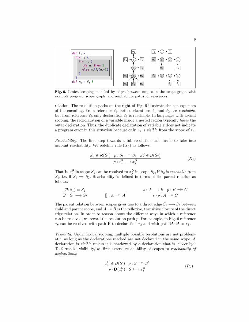
9

1

n8

f1f9

2 f2

3 n3

f6

n4

n7n5

1 f1f9

1

n8

23

n3

n4

1

f1

2

f2

3f6

def f1 = fix f2 { fun n3 { ifz n4 then 1 else n5*f6(n7-1) } }def n8 = f9 5

Fig. 6. Lexical scoping modeled by edges between scopes in the scope graph withexample program, scope graph, and reachability paths for references.

relation. The resolution paths on the right of Fig. 6 illustrate the consequencesof the encoding. From reference f6 both declarations f1 and f2 are reachable,but from reference f9 only declaration f1 is reachable. In languages with lexicalscoping, the redeclaration of a variable inside a nested region typically hides theouter declaration. Thus, the duplicate declaration of variable f does not indicatea program error in this situation because only f2 is visible from the scope of f6.

Reachability. The first step towards a full resolution calculus is to take intoaccount reachability. We redefine rule (X0) as follows:

xRi ∈ R(S1) p : S1� S2 xD

j ∈ D(S2)

p : xRi 7−→ xD

j

(X1)

That is, xRi in scope S1 can be resolved to xD

j in scope S2, if S2 is reachable fromS1, i.e. if S1 � S2. Reachability is defined in terms of the parent relation asfollows:

P(S1) = S2

P : S1 −→ S2 [] : A� A

s : A −→ B p : B� C

s · p : A� C

The parent relation between scopes gives rise to a direct edge S1 −→ S2 betweenchild and parent scope, and A� B is the reflexive, transitive closure of the directedge relation. In order to reason about the different ways in which a referencecan be resolved, we record the resolution path p. For example, in Fig. 6 referencef6 can be resolved with path P to declaration f2 and with path P ·P to f1.

Visibility. Under lexical scoping, multiple possible resolutions are not problem-atic, as long as the declarations reached are not declared in the same scope. Adeclaration is visible unless it is shadowed by a declaration that is ‘closer by’.To formalize visibility, we first extend reachability of scopes to reachability ofdeclarations:

xDi ∈ D(S′) p : S� S′

p ·D(xDi ) : S� xD

i

(R2)

10

That is, a declaration xDi in S′ is reachable from scope S (S� xD

i ), if scope S′is reachable from S.

Given multiple reachable declarations, which one should we prefer? A reach-able declaration xD

i is visible in scope S (S 7−→ xDi ) if there is no other declaration

for the same name that is reachable through a more specific path:

p : S� xDi ∀j, p′(p′ : S� xD

j ⇒ ¬(p′ < p))

p : S 7−→ xDi

(V2)

where the specificity ordering p′ < p on paths is defined as

D(_) < Ps1 < s2

s1 · p1 < s2 · p2

p1 < p2

s · p1 < s · p2

That is, a path with fewer parent transitions is more specific than a path withmore parent transitions. This formalizes the notion that a declaration in a“nearer” scope shadows a declaration in a “farther” scope.

Finally, a reference resolves to a declaration if that declaration is visible inthe scope of the reference.

xRi ∈ R(S) p : S 7−→ xD

j

p : xRi 7−→ xD

j

(X2)

Example. In Fig. 6 the scope (labeled 3) containing reference f6 can reach twodeclarations for f: P ·D(fD

2 ) : S3� fD2 and P ·P ·D(fD

1 ) : S3� fD1 . Since the

first path is more specific than the second path, only f2 is visible, i.e. P ·D(fD2 ) :

S3 7−→ fD2 . Therefore f6 resolves to f2, i.e. P ·D(fD

2 ) : fR6 7−→ fD

2 .

Scopes, revisited. Now that we have defined the notions of reachability andvisibility, we can give a more precise description of the sense in which scopes“behave uniformly” with respect to resolution. For every scope S:

– Each declaration in the program is either visible at every reference in R(S)or not visible at any reference in R(S).

– For each reference in the program, either every declaration in D(S) is reach-able from that reference, or no declaration in D(S) is reachable from thatreference.

– Every declaration in D(S) is visible at every reference in R(S).

2.4 Imports

Introducing modules and imports complicates the name binding picture. Decla-rations are no longer visible only through the lexical context, but may be visiblethrough an import as well. Furthermore, resolving a reference may require firstresolving one or more imports, which may in turn require resolving further im-ports, and so on.

We model an import by means of a reference xRi in the set of imports I(S) of a

scope S. (Imports are also always references and included in some R(S′), but not

11

A2

C10

B7

b9 b11

1

2 3 4a4

b5 c6 B3 C8 c12

2c6 B3 C10 c124B7 3 C8

c1

b13

B7B3 12 C8 C1013

1 c1

def c1 = 4module A2 { import B3 def a4 = b5 + c6}module B7 { import C8 def b9 = 0}module C10 { def b11 = 1 def c12 = b13}

Fig. 7. Modules and imports with example program, scope graph, and reachabilitypaths for references.

necessarily in the same scope in which they are imports.) We model a module byassociating a scope S with a declaration xD

i :S. This associated named scope (i.e.,named by x) represents the declarations introduced by, and encapsulated in, themodule. (We write the :S only in rules where it is required; where we omit it, thedeclaration may or may not have an associated scope.) Thus, importing entailsresolving the import reference to a declaration and making the declarations inthe scope associated with that declaration available in the importing scope.

Note that ‘module’ is not a built-in concept in our framework. A module isany construct that (1) is named, (2) has an associated scope that encapsulatesdeclarations, and (3) can be imported into another scope. Of course, this can beused to model the module systems of languages such as ML. But it can be appliedto constructs that are not modules at first glance. For example, a class in Javaencapsulates class variables and methods, which are imported into its subclassesthrough the ‘extends’ clause. Thus, a class plays the role of module and theextends clause that of import. We discuss further applications in Section 3.

Reachability. To define name resolution in the presence of imports, we firstextend the definition of reachability. We saw above that the parent relation onscopes induces an edge S1 −→ S2 between a scope S1 and its parent scope S2

in the scope graph. Similarly, an import induces an edge S1 −→ S2 between ascope S1 and the scope S2 associated with a declaration imported into S1:

yRi ∈ I(S1) p : yR

i 7−→ yDj :S2

I(yRi , y

Dj :S2) : S1 −→ S2

(I3)

Note the recursive invocation of the resolution relation on the name of the im-ported scope.

Figure 7 illustrates extensions to scope graphs and paths to describe imports.Association of a name to a scope is indicated by an open-headed arrow from thename declaration box to the scope circle. (For example, scope 2 is associated todeclaration A2.) An import into a scope is indicated by an open-headed arrowfrom the scope circle to the import name reference box. (For example, scope 2

12

imports the contents of the scope associated to the resolution of reference B3;note that since B3 is also a reference within scope 2, there is also an ordinaryarrow in the opposite direction, leading to a double-headed arrow in the scopegraph.) Edges in reachability paths representing the resolution of imported scopenames to their definitions are drawn dashed. (For example, reference B3 resolvesto declaration B7, which has associated scope 3.) The paths at the bottom rightof the figure illustrate that the scope (labeled 2) containing reference c6 canreach two declarations for c: P ·D(cD

1 ) : S2 � cD1 and I(BR

3 , BD7 :S3) · I(CR

8 , CD10:

S4) ·D(cD12) : S2� cD

12, making use of the subsidiary resolutions BR3 7−→ BD

7 andCR

8 7−→ CD10.

def a1 = ...module A2 {def a3 = ...def b4 = ...

}module C5 {import A6def b7 = a8def c9 = b10

}

Fig. 8. Parent vsImport

def a1 = ...module B2 {}module C3 {def a4 = ...module D5 {

import B6def e7 = a8

}}

Fig. 9. Parent ofimport

Visibility. Imports cause new kinds of ambiguities in resolu-tion paths, which require extension of the visibility policy.

The first issue is illustrated by Fig. 8. In the scope of ref-erence b10 we can reach declaration b7 with path D(bD

7 ) anddeclaration b4 with path I(AR

6 , AD2 :SA) · D(bD

4 ) (where SAis the scope named by declaration A2). We resolve this con-flict by extending the specificity order with the rule D(_) <I(_,_). That is, local declarations override imported declara-tions. Similarly, in the scope of reference a8 we can reach dec-laration a1 with path P ·D(aD

1 ) and declaration a3 with pathI(AR

6 , AD2 :SA) ·D(aD

3 ). We resolve this conflict by extendingthe specificity order with the rule I(_,_) < P. That is, res-olution through imports is preferred over resolution throughparents. In other words, declarations in imported modulesoverride declarations in lexical parents.

The next issue is illustrated in Fig. 9. In the scope of ref-erence a8 we can reach declaration a4 with path P · D(aD

4 )and declaration a1 with path P · P · D(aD

1 ). The specificityordering guarantees that only the first of these is visible,giving the resolution we expect. However, with the rules asstated so far, there is another way to reach a1, via the pathI(BR

6 , BD2 :SB)·P·D(aD

1 ). That is, we first import module B, andthen go to its lexical parent, where we find the declaration. In other words, whenimporting a module, we import not just its declarations, but all declarations inits lexical context. This behavior seems undesirable; to our knowledge, no reallanguages exhibit it. To rule out such resolutions, we define a well-formednesspredicate WF(p) that requires paths p to be of the form P∗ ·I(_,_)∗, i.e. forbid-ding the use of parent steps after one or more import steps. We use this predicateto restrict the reachable declarations relation by only considering scopes reach-able through a well-formed path:

xDi ∈ D(S′) p : S� S′ WF(p)

p ·D(xDi ) : S� xD

i

(R3)

13

AD2 :SA2 ∈ D(SA1)

AR4 ∈ I(Sroot)

AR4 ∈ R(Sroot) AD

1 :SA1 ∈ D(Sroot)

AR4 7−→ AD

1 :SA1

Sroot −→ SA1 (∗)Sroot� AD

2 :SA2

AR4 ∈ R(Sroot) Sroot 7−→ AD

2 :SA2

AR4 7−→ AD

2 :SA2

Fig. 10. Derivation for AR4 7−→ AD

2 :SA2 in a calculus without import tracking.

The complete definition of well-formed paths and specificity order on paths isgiven in Fig. 2. In Section 2.5 we discuss how alternative visibility policies canbe defined by just changing the well-formedness predicate and specificity order.

module A1 {module A2 {

def a3 = ...}

}import A4def b5 = a6

Fig. 11. Self im-port

module A1 {module B2 {

def x3 = 1}

}module B4 {

module A5 {def y6 = 2

}}module C7 {

import A8import B9def z10 = x11

+ y12}

Fig. 12. Anoma-lous resolution

Seen imports. Consider the example in Fig. 11. Is declarationa3 reachable in the scope of reference a6? This reduces to thequestion whether the import of A4 can resolve to moduleA2. Surprisingly, it can, in the calculus as discussed so far,as shown by the derivation in Fig. 10 (which takes a fewshortcuts). The conclusion of the derivation is that AR

4 7−→AD

2 :SA2 . This conclusion is obtained by using the import at A4

to conclude at step (*) that Sroot −→ SA1, i.e. that the body

of module A1 is reachable! In other words, the import of A4

is used in its own resolution. Intuitively, this is nonsensical.To rule out this kind of behavior we extend the calculus

to keep track of the set of seen imports I using judgementsof the form I ` p : xR

i 7−→ xDj . We need to extend all rules to

pass the set I, but only the rules for resolution and importare truly affected:

xRi ∈ R(S) {xR

i } ∪ I ` p : S 7−→ xDj

I ` p : xRi 7−→ xD

j

(X)

yRi ∈ I(S1) \ I I ` p : yR

i 7−→ yDj :S2

I ` I(yRi , y

Dj :S2) : S1 −→ S2

(I)

With this final ingredient, we reach the full calculus inFig. 3. It is not hard to see that the resolution relation iswell-founded. The only recursive invocation (via the I rule)uses a strictly larger set I of seen imports (via the X rule); since the set R(G)is finite, I cannot grow indefinitely.

Anomalies. Although the calculus produces the desired resolutions for a widevariety of real language constructs, its behavior can be surprising on corner cases.Even with the “seen imports” mechanism, it is still possible for a single derivation

14

to resolve a given import in two different ways, leading to unintuitive results.For example, in the program in Fig. 12, x11 can resolve to x3 and y12 can resolveto y6. (Derivations left as an exercise to the curious reader!) In our experience,phenomena like this occur only in the presence of mutually-recursive imports; toour knowledge, no real language has these (perhaps for good reason). We deferdeeper exploration of these anomalies to future work.

2.5 Variants

The resolution calculus presented so far reflects a number of binding policydecisions. For example, we enforce imports to be transitive and local declarationsto be preferred over imports. However, not every language behaves like this. Wenow present how other common behaviors can easily be represented with slightmodifications of the calculus. Indeed, the modifications do not have to be doneon the calculus itself (the −→, � , � and 7−→ relations) but can simply beencoded in the WF predicate and the < ordering on paths.

Reachability policy. Reachability policies define how a reference can access aparticular definition, i.e. what rules can be used during the resolution. We canchange our reachability policy by modifying the WF predicate. For example, ifwe want to rule out transitive imports, we can change WF to be

WF(p)⇔ p ∈ P∗ · I(_,_)?

where ? denotes the at most one operation on regular expressions. Therefore, animport can only be used once at the end of the chain of scopes.

For a language that supports both transitive and non-transitive imports, wecan add a label on references corresponding to imports. If xR is a referencerepresenting a non-transitive import and xTR a reference corresponding to atransitive import, then the WF predicate simply becomes:

WF(p)⇔ p ∈ P∗ · I(_TR,_)∗ · I(_R,_)?

module A1 {def x2 = 3

}module B3 {include A4;def x5 = 6;def z6 = x7

}

Fig. 13. Include

Now no import can occur after the use of a non-transitive one.Similarly, we can modify the rule to handle the Export

declaration in Coq, which forces transitivity (a resolution canalways use an exported module even after importing from anon-transitive one). Assume xR is a reference representing anon-transitive import and xER a reference corresponding to anexport; then we can use the following predicate:

WF(p)⇔ p ∈ P∗ · I(_R,_)? · I(_ER,_)∗

Visibility policy. We can modify the visibility policy, i.e. how resolutions shadoweach other, by changing the definition of the specificity ordering. For example,we might want imports to act like textual inclusion, so the declarations in theincluded module have the same precedence as local declarations. This is similarto Standard ML’s include mechanism. In the program in Fig. 13, the referencex7 should be treated as having duplicate resolutions, to either x5 or x2; the

15

1

2

b2a1 c3

a4

b6

c12a10 b11

c5

b9

a7

c8

def a1 = 0def b2 = 1def c3 = 2

letpar a4 = c5 b6 = a7 c8 = b9in a10+b11+c12

1

b2a1 c3

a4

b6

c12a10 b11

c5

b9

a7

c8

2

def a1 = 0def b2 = 1def c3 = 2

letrec a4 = c5 b6 = a7 c8 = b9in a10+b11+c12

1

b2a1 c3

a4

b6

c12a10 b11

c5

b9

a7

c8

2

4

3

def a1 = 0def b2 = 1def c3 = 2

let a4 = c5 b6 = a7 c8 = b9in a10+b11+c12

Fig. 14. Example LM programs with sequential, recursive, and parallel let, and theirencodings as scope graphs.

former should not hide the latter. To handle this situation, we can drop the ruleD(_) < I(_,_) so that definitions and references will get the same precedence,and a definition will not shadow an imported definition. To handle both includeand ordinary imports, we can once again differentiate the references, and definedifferent ordering rules depending on the reference used in the import step.

3 Coverage

To what extent does the scope graph framework cover name binding systemsthat live in the world of real programming languages? It is not possible to provecomplete coverage by the framework, in the sense of being able to encode all pos-sible name binding systems that exist or may be designed in the future. (Indeed,given that these systems are typically implemented in compilers with algorithmsin Turing-complete programming languages, the framework is likely not to becomplete.) However, we believe that our approach handles many lexically-scopedlanguages. The design of the framework was informed by an investigation of awide range of name binding patterns in existing languages, their (attempted)formalization in the NaBL name binding language [14, 16], and their encodingin scope graphs. In this section, we discuss three such examples: let bindings,qualified names, and inheritance in Java. This should provide the reader with agood sense of how name binding patterns can be expressed using scope graphs.Appendix A of [19] provides further examples, including definition-before-use,compilation units and packages in Java, and namespaces and partial classes inC#.

Let bindings. The several flavors of let bindings in languages such as ML,Haskell, and Scheme do not follow the unary lexical binding pattern in which thebinding construct dominates the abstract syntax tree that makes up its scope.The LM language from Fig. 4 has three flavors of let bindings: sequential,recursive, and parallel let, each with a list of bindings and a body expression.Fig. 14 shows the encoding into scope graphs for each of the constructs andmakes precise how the bindings are interpreted in each flavour. In the recursive

16

1

2

3 5c3

f7

B1

C2 D6

D4

4 f5

module B1 { module C2 { def c3 = D4.f5(3) } module D6 { def f7 = ... }}

Fig. 15. Example LM program withpartially-qualified name.

3

2

1

C4

C1

4

D3E7

D8

f2

g5

f6

f9

g10f12 h11

class C1 { int f2 = 42;}class D3 extends C4 { int g5 = f6; }class E7 extends D8 { int f9 = g10; int h11 = f12; }

Fig. 16. Class inheritance in Java modeledby import edges.

letrec, the bindings are visible in all initializing expressions, so a single scopesuffices for the whole construct. In the sequential let, each binding is visible inthe subsequent bindings, but not in its own initializing expression. This requiresthe introduction of a new scope for each binding. In the parallel letpar, thevariables being bound are not visible in any of the initializing expressions, butonly in the body. This is expressed by means of a single scope (2) in which thebindings are declared; any references in the initializing expressions are associatedto the parent scope (1).

Qualified names. Qualified names refer to declarations in named scopes outsidethe lexical scoping. They can be either used as simple references or as imports.For example, fully-qualified names of Java classes can be used to refer to (orimport) classes from other packages. While fully-qualified names allow navigatingnamed scopes from the root scope, partially-qualified names give access to lexicalsubscopes, which are otherwise hidden from lexical parent scopes.

The LM program in Fig. 15 uses a partially-qualified name D.f to accessfunction f in submodule D. We can model this pattern using an anonymousscope (4), which is not linked to the lexical context. The relative name (f5) is areference in the anonymous scope. We add the qualifying scope name (D4) as animport in the anonymous scope.

Inheritance in Java. We can model inheritance in object-oriented languageswith named scopes and imports. For example, Fig. 16 shows a hierarchy of threeJava classes. Class C declares a field f. Class D extends C and inherits its fieldf. Class E extends D, inheriting the fields of C and D. Each class name is adeclaration in the same package scope (1), and associated with the scope of itsclass body. Inheritance is modeled with imports: a subclass body scope containsan import referring to its super class, making the declarations in the super classreachable from the body. In the example, the scope (4) representing the bodyof class E contains an import referring to its super class D. Using this import,g10 correctly resolves to g5 . Since local declarations hide imported declarations,f12 also refers correctly to the local declaration f9, which hides the transitively

17

[[ds]]prog := let S := new⊥ in [[ds]]recdS

[[d ds]]recdS := [[d]]decS ; [[ds]]recdS

[[]]recdS := ()

[[module xi{ds}]]decS := let S′ := newS in D(S) += xD

i :S′; [[ds]]recdS′

[[import xs]]decS := [[xs]]rqidS ; [[xs]]iqidS

[[def xi = e]]decS := D(S) += xDi ; [[e]]

expS

[[xs]]expS := [[xs]]rqidS

[[(fun | fix) xi{e}]]expS := let S′ := newS in D(S′) += xD

i ; [[e]]expS′

[[letrec bs in e]]expS := let S′ := newS in [[bs]]recbS′ ; [[e]]expS′

[[letpar bs in e]]expS := let S′ := newS in [[bs]]parb(S,S′); [[e]]expS′

[[let bs in e]]expS := let S′ := [[bs]]seqbS in [[e]]expS′

[[e1 e2]]expS := [[e1]]

expS ; [[e2]]

expS

[[e1 ⊕ e2]]expS := [[e1]]

expS ; [[e2]]

expS

[[n]]expS := ()

[[xi.xs]]rqidS := R(S) += xR

i ; let S′ := new⊥ in I(S′) += xRi ; [[xs]]

rqidS′

[[xi]]rqidS := R(S) += xR

i

[[xi.xs]]iqidS := [[xs]]iqidS

[[xi]]iqidS := I(S) += xR

i

[[xi = e; bs]]recbS := D(S) += xDi ; [[e]]

expS ; [[bs]]recbS

[[]]recbS := ()

[[xi = e; bs]]parb(S,S′) := D(S′) += xDi ; [[e]]

expS ; [[bs]]parb(S,S′)

[[]]parb(S,S′) := ()

[[xi = e; bs]]seqbS := [[e]]expS ; let S′ := newS in D(S′) += xDi ; ret(S′)

[[]]seqbS := ret(S)

Fig. 17. Scope graph construction for LM via syntax-directed AST traversal.

imported f2. Note that since a scope can contain several imports, encodingmultiple inheritance uses exactly the same principle.

4 Scope Graph Construction

The preceding sections have illustrated scope graph construction by means ofexamples corresponding to various language features. Of course, to apply ourformalism in practice, one must be able to construct scope graphs systemati-cally. Ultimately, we would like to be able to specify this process for arbitrarylanguages using a generic binding specification language such as NaBL [16], butthat remains future work. Here we illustrate systematic scope graph constructionfor arbitrary programs in a specific language, LM (Fig. 4), via straightforwardsyntax-directed traversal.

Figure 17 describes the construction algorithm. For clarity of presentation,the algorithm traverses the program’s concrete syntax; a real implementationwould traverse the program’s AST. The algorithm is presented in an ad hoc

18

imperative language, explained here. The traversal is specified as a collection of(potentially) mutually recursive functions, one or more for each syntactic classof LM. Each function f is defined by a set of clauses [[pattern]]fargs. When f isinvoked on a term, the clause whose pattern matches the term is executed. Func-tions may also take additional arguments args. Each clause body consists of asequence of statements separated by semicolons. Functions can optionally returna value using ret(). The let statement binds a metavariable in the remainder ofthe clause body. An empty clause body is written ().

The algorithm is initiated by invoking [[_]]prog on an entire LM program. Itsnet effect is to produce a scope graph via a sequence of imperative operations.The construct newP creates a new scope S with parent P (or no parent if p =⊥)and empty sets D(S), R(S), and I(S). These sets are subsequently populatedusing the += operator, which extends a set imperatively. The program scopegraph is simply the set of scopes that have been created and populated whenthe traversal terminates.

5 Resolution Algorithm

The calculus of Section 2 gives a precise definition of resolution. In principle, wecan search for derivations in the calculus to answer questions such as “Does thisvariable reference resolve to this declaration?” or “Which variable declarationsdoes this reference resolve to?” But automating this search process is not trivial,because of the need for back-tracking and because the paths in reachabilityderivations can have cycles (visiting the same scope more than once), and hencecan grow arbitrarily long.

In this section we describe a deterministic and terminating algorithm forcomputing resolutions, which provides a practical basis for implementing toolsbased on scope graphs, and prove that it is sound and complete with respectto the calculus. This algorithm also connects the calculus, which talks aboutresolution of a single variable at a time, to more conventional descriptions ofbinding which use “environments” or “contexts” to describe all the visible orreachable declarations accessible from a program location.

For us, an environment is just a set of declarations xDi . This can be thought

of as a function from identifiers to (possible empty) sets of declaration positions.(In this paper, we leave the representation of environments abstract; in practice,one would use a hash table or other dictionary data structure.) We construct anatomic environment corresponding to the declarations in each scope, and thencombine atomic environments to describe the sets of reachable and visible dec-larations resulting from the parent and import relations. The key operator forcombining environments is shadowing, which returns the union of the declara-tions in two environments restricted so that if a variable x has any declarationsin the first environment, no declarations of x are included from the second envi-ronment. More formally:

Definition 1 (Shadowing). For any environments E1, E2, we write:E1 / E2 := E1 ∪ {xD

i ∈ E2 | @ xDi′ ∈ E1}

19

Res[I](xRi ) := {xD

j | ∃S s.t. xRi ∈ R(S) ∧ xD

j ∈ EnvV [{xRi } ∪ I, ∅](S)}

EnvV [I, S](S) := EnvL[I, S](S) / EnvP [I, S](S)EnvL[I, S](S) := EnvD[I, S](S) / EnvI [I, S](S)

EnvD[I, S](S) :=

{∅ if S ∈ SD(S)

EnvI [I, S](S) :=

∅ if S ∈ S⋃{EnvL[I, {S} ∪ S](Sy) | yR

i ∈ I(S) \ I ∧ yDj :Sy ∈ Res[I](yR

i )}

EnvP [I, S](S) :=

{∅ if S ∈ SEnvV [I, {S} ∪ S](P(S))

Fig. 18. Resolution algorithm

Figure 18 specifies an algorithm Res[I](xRi ) for resolving a reference xR

i to a set ofcorresponding declarations xD

j . Like the calculus, the algorithm avoids trying touse an import to resolve itself by maintaining a set I of “already seen” imports.The algorithm works by computing the full environment EnvV [I,S](S) of decla-rations that are visible in the scope S containing xR

i , and then extracting justthe declarations for x. The full environment, in turn, is built from the more basicenvironments EnvD of immediate declarations, EnvI of imported declarations,and EnvP of lexically enclosing declarations, using the shadowing operator. Theorder of construction matches both the WF restriction from the calculus, whichprevents the use of parent after an import, and the path ordering <, whichprefers immediate declarations over imports and imports over declarations fromthe parent scope. (Note that the algorithm does not work for the variants of WFand < described in Section 2.5.) A key difference from the calculus is that theshadowing operator is applied at each stage in environment construction, ratherthan applying the visibility criterion just once at the “top level” as in calculusrule V . This difference is a natural consequence of the fact that the algorithmcomputes sets of declarations rather than full derivation paths, so it does notmaintain enough information to delay the visibility computation.

Termination The algorithm is terminating using the well-founded lexicographicmeasure (|R(G) \ I|, |S(G) \ S|). Termination is straightforward by unfolding thecalls to Res in EnvI and then inlining the definitions of EnvV and EnvL: thisgives an equivalent algorithm in which the measure strictly decreases at everyrecursive call.

5.1 Correctness of Resolution Algorithm

The resolution algorithm is sound and complete with respect to the calculus.

Theorem 1. ∀ I, xRi , j, (x

Dj ∈ Res[I](xR

i )) ⇐⇒ (∃p s.t. I ` p : xRi 7−→ xD

j ).

We sketch the proof of this theorem here; details of the supporting lemmasand proofs are in Appendix B of [19]. To begin with, we must deal with the

20

Transitive closureI, S ` [] : A� A

(N ′)

I ` s : A −→ B B 6∈ S I, {B} ∪ S ` p : B� C

I, S ` s · p : A� C(T ′)

Reachable declarations

xDi ∈ D(S′) S 6∈ S I, {S} ∪ S ` p : S� S′ WF(p)

I, S ` p ·D(xDi ) : S� xD

i

(R′)

Visible declarations

I, S ` p : S� xDi ∀j, p′(I, S ` p′ : S� xD

j ⇒ ¬(p′ < p))

I, S ` p : S 7−→ xDi

(V ′)

Reference resolution

xRi ∈ R(S) {xR

i } ∪ I, ∅ ` p : S 7−→ xDj

I ` p : xRi 7−→ xD

j

(X ′)

Fig. 19. “Primed” resolution calculus with “seen scopes” component

fact that the calculus can generate reachability derivations with cycles, but thealgorithm does not follow cycles. In fact, visibility derivations cannot have cycles:

Lemma 1. If I ` p : xRi 7−→ xD

j then p is cycle-free.

We therefore begin by defining an alternative version of the calculus that preventsconstruction of cyclic paths. This alternative calculus consists of the original rules(P ), (I) from Figure 3 together with the new rules (N ′), (T ′), (R′), (V ′), (X ′)from Figure 19. The new rules describe transitions that include a “seen scopes”component S which is used to enforce acyclicity of paths. By inspection, thisis the only difference between the “primed” system and original one. Thus, byLemma 1, we have

Lemma 2. ∀I,S, xDi , (∃p s.t. I ` p : S 7−→ xD

i ) ⇐⇒ (∃p s.t. I, ∅ ` p : S 7−→ xDi ).

Hereinafter, we can work with the primed system.Next we define a family of sets P of derivable paths in the (primed) calculus.

Definition 2 (Path Sets).

PD[I,S](S) := {p | ∃ xDi s.t. p = D(xD

i ) ∧ I,S ` p : S � xDi }

PP [I,S](S) := {p | ∃ p′ xDi s.t. p = P · p′∧

I,S ` p : S � xDi ∧ I, {S} ∪ S ` p′ : P(S) 7−→ xD

i }PI [I,S](S) := {p | ∃ p′ xD

i yRj y

Dj′:S′ s.t. p = I(yR

j , yDj′:S′) · p′∧

I,S ` p : S � xDi ∧ I, {S} ∪ S ` p′ : S′ 7−→ xD

i }PL[I,S](S) := {p | ∃ xD

i s.t. I,S ` p : S 7−→ xDi ∧ p ∈ I(_,_)∗ ·D(_)}

PV [I,S](S) := {p | ∃ xDi s.t. I,S ` p : S 7−→ xD

i }

21

These sets are designed to correspond to the various classes of environmentsEnvC . PD, PP , and PI contain all reachability derivations starting with a D(_),P, or I(_,_) respectively, with the further condition that the tail of each deriva-tion is a visibility derivation (i.e. is most specific among all reachability deriva-tions). PV describes the set of all visibility derivations. (PL is similar, but omitspaths including P steps, because well-formedness prevents using these steps af-ter an import step.) For compactness, we state the key result uniformly over allclasses of sets:

Definition 3. For any path p, δ(p) := xDi iff ∃p′ s.t. p = p′ ·D(xD

i ) and for anyset of paths P , ∆(P ) := {δ(p) | p ∈ P}.

Lemma 3. For each class C ∈ {V,L,D, I, P}:

∀ I S S,Envc[I,S](S) = ∆(PC [I,S](S))

Proof. We first prove two auxiliary lemmas about reachability and visibility afterone step:

∀ I S s p S xDi , (I,S ` s · p ·D(xD

i ) : S� xDi =⇒ I, {S}∪S ` s : S −→ S′ =⇒

I, {S} ∪ S ` p ·D(xDi ) : S′� xD

i ) (♦)

∀ I S s p S xDi , (I,S ` s · p : S 7−→ xD

i =⇒ I, {S} ∪ S ` s : S −→ S′ =⇒I, {S} ∪ S ` p : S′ 7−→ xD

i ) (�)

Then we proceed by three nested inductions, the outer one on I (or, more strictly,on |R(G) \ I|, the number of references not in I), the second one on S (morestrictly, on |S(G) \ S|, the number of scopes not in S) and the third one on theclass C with the order V > L > P, I,D. Then we conclude using ♦ and � and anumber of other technical results. Details are in Appendix B of [19]. ut

With these lemmas in hand we proceed to prove Theorem 1.

Proof. Fix I, xRi , and j. Given S, the (unique) scope such that xR

i ∈ R(S):xDj ∈ Res[xR

i ](I)⇔ xDj ∈ EnvV [{xR

i } ∪ I, ∅](S)By the V case of Lemma 3 and the definition of PS , this is equivalent to

∃p s.t. {xRi } ∪ I, ∅ ` p : S 7−→ xD

j

which, by Lemma 2 and rule X, is equivalent to ∃p s.t. I ` p : xRi 7−→ xD

j . ut

6 α-equivalence and Renaming

The choice of a particular name for a bound identifier should not affect themeaning of a program. This notion of name irrelevance is usually referred to asα-equivalence, but definitions of α-equivalence exist only for some languages andare language-specific. In this section we show how the scope graph and resolutioncalculus can be used to specify α-equivalence in a language-independent way.

22

Free variables. A free variable is a reference that does not resolve to any decla-ration (xR

i is free if @ j, p s.t. I ` p : xRi 7−→ xD

j ); a bound variable has at leastone declaration. For uniformity, we introduce for each possibly free variable x aprogram-independent artificial declaration xD

x̄ with an artificial position x̄. Thesedeclarations do not belong to any scope but are reachable through a particularwell-formed path >, which is less specific than any other path, according to thefollowing rules:

I ` > : S� xDx̄

p 6= >p < >

This path representing the resolution of a free reference is shadowed by anyexisting path leading to a concrete declaration; therefore the resolution of boundvariables is unchanged.

6.1 α-Equivalence

We now define α-equivalence using scope graphs. Except for the leaves represent-ing identifiers, two α-equivalent programs must have the same abstract syntaxtree. We write P ' P’ (pronounced “P and P’ are similar”) when the ASTs of Pand P’ are equal up to identifiers. To compare two programs we first comparetheir AST structures; if these are similar then we compare how identifiers be-have in these programs. Since two potentially α-equivalent programs are similar,the identifiers occur at the same positions. In order to compare the identifiers’behavior, we define equivalence classes of positions of identifiers in a program:positions in the same equivalence class are declarations of, or references to, thesame entity. The abstract position x̄ identifies the equivalence class correspond-ing to the free variable x.

Given a program P, we write P for the set of positions corresponding toreferences and declarations and PX for P extended with the artificial positions(e.g. x̄). We define the P∼ equivalence relation between elements of PX as thereflexive symmetric and transitive closure of the resolution relation.

Definition 4 (Position equivalence).

I ` p : xRi 7−→ xD

i′

iP∼ i′

i′P∼ i

iP∼ i′

iP∼ i′ i′

P∼ i′′

iP∼ i′′ i

P∼ i

In this equivalence relation, the class containing the abstract free variable dec-laration cannot contain any other declaration. So the references in a particularclass are either all free or all bound.

Lemma 4 (Free variable class). The equivalence class of a free variable doesnot contain any other declaration, i.e. ∀ xD

i , iP∼ x̄ =⇒ i = x̄

Proof. Detailed proof is in Appendix B of [19]. We first prove:∀ xR

i , (I ` > : xRi 7−→ xD

x̄ ) =⇒ ∀ p i′, I ` p : xRi 7−→ xD

i′ =⇒ i′ = x̄ ∧ p = >and then proceed by induction on the equivalence relation.

23

The equivalence classes defined by this relation contain references to or decla-rations of the same entity. Given this relation, we can state that two programsare α-equivalent if the identifiers at identical positions refer to the same entity,that belong to the same equivalence class:

Definition 5 (α-equivalence). Two programs P1 and P2 are α-equivalent (de-noted P1

α≈ P2) when they are similar and have the same ∼-equivalence classes:

P1α≈ P2 , P1 ' P2 ∧ ∀ i i′, i P1∼ i′ ⇔ i

P2∼ i′

Remark 1.α≈ is an equivalence relation since ' and⇔ are equivalence relations.

Free variables. The P∼ equivalence classes corresponding to free variables x alsocontain the artificial position x̄. Since the equivalence classes of two equivalentprograms P1 and P2 have to be exactly the same, every element equivalent tox̄ (i.e. a free reference) in P1 is also equivalent to x̄ in P2. Therefore the freereferences of α-equivalent programs have to be identical.

Duplicate declarations. The definition allows us to also capture α-equivalence ofprograms with duplicate declarations. Assume that a reference xR

i1resolves to

two definitions xDi2

and xDi3; then i1, i2 and i3 belong to the same equivalence

class. Thus all α-equivalent programs will have the same ambiguities.

6.2 Renaming

Renaming is the substitution of a bound variable by a new variable throughoutthe program. It has several practical applications such as rename refactoring inan IDE, transformation to a program with unique identifiers, or as an interme-diate transformation when implementing capture-avoiding substitution.

A valid renaming should respect α-equivalence classes. To formalize this ideawe first define a generic transformation scheme on programs that also dependson the position of the sub-term to rewrite:

Definition 6 (Position dependent rewrite rule). Given a program P, wedenote by (ti → t′ | F ) the transformation that replaces the occurrences of thesub-term t at positions i by t′ if the condition F is true. (T )P denotes the appli-cation of the transformation T to the program P.

Given this definition we can now define the renaming transformation that re-places the identifier corresponding to an entire equivalence class:

Definition 7 (Renaming). Given a program P and a position i correspondingto a declaration or a reference for the name x, we denote by [xi:=y]P the programP’ corresponding to P where all the identifiers x at positions P∼-equivalent to iare replaced by y:

[xi := y]P , (xi′ → y | i′ P∼ i)P

24

However, not every renaming is acceptable: a renaming might provoke variablecaptures and completely change the meaning of a program.

Definition 8 (Valid renamings). Given a program P, renaming [xi := y] isvalid only if it produces an α-equivalent program, i.e. [xi := y]P

α≈ P

Remark 2. This definition prevents the renaming of free variables since α-equivalentprograms have exactly the same free variables.

Intuitively, valid renamings are those that do not accidentally “capture” vari-ables. Since the capture of a reference resolution also depends on the seen-importcontext in which this resolution occurs, a precise characterization of capture inour general setting is complex and we leave it for future work.

7 Related Work

Binding-sensitive program representations. There has been a great deal of workon representing program syntax in ways that take explicit note of binding struc-ture, usually with the goal of supporting program transformation or mechanizedreasoning tools that respect α-equivalence by construction. Notable techniquesinclude de Bruijn indexing [7], Higher-Order Abstract Syntax (HOAS) [20], lo-cally nameless representations [3], and nominal sets [10]. (Aydemir, et al. [2] givea survey in the context of mechanized reasoning.) However, most of this workhas concentrated on simple lexical binding structures, such as single-argumentλ-terms. Cheney [4] gives a catalog of more interesting binding patterns andsuggests how nominal logic can be used to describe many of them. However, heleaves treatment of module imports as future work.

Binding specification languages. The Ott system [22] allows definition of syntax,name binding and semantics. This tool generates language definitions for theo-rem provers along with a notion of α-equivalence and functions such as capture-avoiding substitution that can be proven correct in the chosen proof assistantmodulo α-equivalence. Avoiding capture is also the basis of hygienic macros inScheme. Dybvig [8] gives an algorithmic description of what hygiene means.Herman and Wand [13, 12] introduce static binding specifications to formalizea notion of α-equivalence that does not depend on macro expansion. Stansiferand Wand’s Romeo system [23] extends these specifications to somewhat moreelaborate binding forms, such as sequential let. Unbound [25] is another re-cent domain specific language for describing bindings that supports moderatelycomplex binding forms. Again, none of these systems treat modules or imports.

Language engineering. In language engineering approaches, name bindings areoften realized using a random-access symbol table such that multiple analysisand transformation stages can reuse the results of a single name resolution pass[1]. Another approach is to represent the result of name resolution by meansof reference attributes, direct pointers from the uses of a name to its definition

25

[11]. However these representations are usually built using an implementationof a language-specific resolution algorithm. Erdweg, et al. [9] describe a systemfor defining capture-free transformations, assuming resolution algorithms areprovided for the source and target languages. The approach represents the resultof name resolution using ‘name graphs’ that map uses to definitions (referencesto declarations in our terminology) and are language independent. This notionof ‘name graph’ inspired our notion of ‘scope graph’. The key difference is thatthe results of name resolution generated by the resolution calculus are paths thatextend a use-def pair with the language-independent evidence for the resolution.

Semantics engineering. Semantics engineering approaches to name binding varyfrom first-order representation with substitution [15], to explicit or implicit en-vironment propagation [21, 18, 6], to HOAS [5]. Identifier bindings representedwith environments are passed along in derivation rules, rediscovering bindingsfor each operation. This approach is inconvenient for more complex patternssuch as mutually recursive definitions.

8 Conclusion and Future Work

We have introduced a generic, language-independent framework for describingname binding in programming languages. Its theoretical basis is the notion ofa scope graph, which abstracts away from syntax, together with a calculus forderiving resolution paths in the graph. Scope graphs are expressive enough todescribe a wide range of binding patterns found in real languages, in particularthose involving modules or classes. We have presented a practical resolutionalgorithm, which is provably correct with respect to the resolution calculus. Wecan use the framework to define generic notions of α-equivalence and renaming.

As future work, we plan to explore and extend the theory of scope graphs,in particular to find ways to rule out anomalous examples and to give precisecharacterizations of variable capture and substitution. On the practical side, wewill use our formalism to give a precise semantics to the NaBL DSL, and verify(using proof and/or testing) that the current NaBL implementation conforms tothis semantics.

Our broader vision is that of a complete language designer’s workbench thatincludes NaBL as the domain-specific language for name binding specificationand also includes languages for type systems and dynamic semantics specifica-tions. In this setting, we also plan to study the interaction of name resolutionand types, including issues of dependent types and name disambiguation basedon types. Eventually we aim to derive a complete mechanized meta-theory forthe languages defined in this workbench and to prove the correspondence be-tween static name binding and name binding in dynamics semantics as outlinedin [24].

Acknowledgments We thank the many people who reacted to our previous workon NaBL by asking “but what is its semantics?”; this paper provides our an-swer. We thank the anonymous reviewers for their feedback on previous versions

26

of this paper. This research was partially funded by the NWO VICI LanguageDesigner’s Workbench project (639.023.206). Andrew Tolmach was partly sup-ported by a Digiteo Chair at Laboratoire de Recherche en Informatique, Univer-sité Paris-Sud.

References

1. A. V. Aho, R. Sethi, and J. D. Ullman. Compilers: Principles, Techniques, andTools. Addison-Wesley, 1986.

2. B. E. Aydemir, A. Charguéraud, B. C. Pierce, R. Pollack, and S. Weirich. Engi-neering formal metatheory. In G. C. Necula and P. Wadler, editors, Proceedings ofthe 35th ACM SIGPLAN-SIGACT Symposium on Principles of Programming Lan-guages, POPL 2008, San Francisco, California, USA, January 7-12, 2008, pages3–15. ACM, 2008.

3. A. Charguéraud. The locally nameless representation. Journal of Automated Rea-soning, 49(3):363–408, 2012.

4. J. Cheney. Toward a general theory of names: binding and scope. In R. Pol-lack, editor, ACM SIGPLAN International Conference on Functional Program-ming, Workshop on Mechanized reasoning about languages with variable binding,MERLIN 2005, Tallinn, Estonia, September 30, 2005, pages 33–40. ACM, 2005.

5. A. J. Chlipala. A verified compiler for an impure functional language. InM. V. Hermenegildo and J. Palsberg, editors, Proceedings of the 37th ACMSIGPLAN-SIGACT Symposium on Principles of Programming Languages, POPL2010, Madrid, Spain, January 17-23, 2010, pages 93–106. ACM, 2010.

6. M. Churchill, P. D. Mosses, and P. Torrini. Reusable components of semantic spec-ifications. In W. Binder, E. Ernst, A. Peternier, and R. Hirschfeld, editors, 13thInternational Conference on Modularity, MODULARITY ’14, Lugano, Switzer-land, April 22-26, 2014, pages 145–156. ACM, 2014.

7. N. G. de Bruijn. Lambda calculus notation with nameless dummies, a tool forautomatic formula manipulation, with application to the Church-Rosser theorem.Indagationes Mathematicae, 34(5):381–392, 1972.

8. R. K. Dybvig, R. Hieb, and C. Bruggeman. Syntactic abstraction in scheme.Higher-Order and Symbolic Computation, 5(4):295–326, 1992.

9. S. Erdweg, T. van der Storm, and Y. Dai. Capture-avoiding and hygienic programtransformations. In R. Jones, editor, ECOOP 2014 - Object-Oriented Programming- 28th European Conference, Uppsala, Sweden, July 28 - August 1, 2014. Proceed-ings, volume 8586 of Lecture Notes in Computer Science, pages 489–514. Springer,2014.

10. M. Gabbay and A. M. Pitts. A new approach to abstract syntax with variablebinding. Formal Asp. Comput., 13(3-5):341–363, 2002.

11. G. Hedin and E. Magnusson. Jastadd–an aspect-oriented compiler constructionsystem. Science of Computer Programming, 47(1):37–58, 2003.

12. D. Herman. A Theory of Hygienic Macros. PhD thesis, Northeastern University,Boston, Massachusetts, May 2010.

13. D. Herman and M. Wand. A theory of hygienic macros. In S. Drossopoulou,editor, Programming Languages and Systems, 17th European Symposium on Pro-gramming, ESOP 2008, Held as Part of the Joint European Conferences on The-ory and Practice of Software, ETAPS 2008, Budapest, Hungary, March 29-April6, 2008. Proceedings, volume 4960 of Lecture Notes in Computer Science, pages48–62. Springer, 2008.

27

14. L. C. L. Kats and E. Visser. The Spoofax language workbench: rules for declarativespecification of languages and IDEs. In W. R. Cook, S. Clarke, and M. C. Rinard,editors, Proceedings of the 25th Annual ACM SIGPLAN Conference on Object-Oriented Programming, Systems, Languages, and Applications, OOPSLA 2010,pages 444–463, Reno/Tahoe, Nevada, 2010. ACM.

15. C. Klein, J. Clements, C. Dimoulas, C. Eastlund, M. Felleisen, M. Flatt, J. A.McCarthy, J. Rafkind, S. Tobin-Hochstadt, and R. B. Findler. Run your research:on the effectiveness of lightweight mechanization. In J. Field and M. Hicks, editors,Proceedings of the 39th ACM SIGPLAN-SIGACT Symposium on Principles ofProgramming Languages, POPL 2012, Philadelphia, Pennsylvania, USA, January22-28, 2012, pages 285–296. ACM, 2012.

16. G. D. P. Konat, L. C. L. Kats, G. Wachsmuth, and E. Visser. Declarative namebinding and scope rules. In K. Czarnecki and G. Hedin, editors, Software Lan-guage Engineering, 5th International Conference, SLE 2012, Dresden, Germany,September 26-28, 2012, Revised Selected Papers, volume 7745 of Lecture Notes inComputer Science, pages 311–331. Springer, 2012.

17. X. Leroy, D. Doligez, A. Frisch, J. Garrigue, D. Rémy, and J. Vouillon. The OCamlsystem (release 4.00): Documentation and user’s manual. Institut National deRecherche en Informatique et en Automatique, July 2012.

18. P. D. Mosses. Modular structural operational semantics. Journal of Logic andAlgebraic Programming, 60-61:195–228, 2004.

19. P. Neron, A. P. Tolmach, E. Visser, and G. Wachsmuth. A theory of name resolu-tion with extended coverage and proofs. Technical Report TUD-SERG-2015-001,Software Engineering Research Group. Delft University of Technology, January2015. Extended version of this paper.

20. F. Pfenning and C. Elliott. Higher-order abstract syntax. In R. L. Wexelblat, edi-tor, Proceedings of the ACM SIGPLAN’88 Conference on Programming LanguageDesign and Implementation (PLDI), Atlanta, Georgia, USA, June 22-24, 1988,pages 199–208. ACM, 1988.

21. B. C. Pierce. Types and Programming Languages. MIT Press, Cambridge, Mas-sachusetts, 2002.

22. P. Sewell, F. Z. Nardelli, S. Owens, G. Peskine, T. Ridge, S. Sarkar, and R. Strnisa.Ott: Effective tool support for the working semanticist. Journal of FunctionalProgramming, 20(1):71–122, 2010.

23. P. Stansifer and M. Wand. Romeo: a system for more flexible binding-safe pro-gramming. In J. Jeuring and M. M. T. Chakravarty, editors, Proceedings of the 19thACM SIGPLAN international conference on Functional programming, Gothenburg,Sweden, September 1-3, 2014, pages 53–65. ACM, 2014.

24. E. Visser, G. Wachsmuth, A. P. Tolmach, P. Neron, V. A. Vergu, A. Passalaqua,and G. D. P. Konat. A language designer’s workbench: A one-stop-shop for imple-mentation and verification of language designs. In A. P. Black, S. Krishnamurthi,B. Bruegge, and J. N. Ruskiewicz, editors, Onward! 2014, Proceedings of the 2014ACM International Symposium on New Ideas, New Paradigms, and Reflections onProgramming & Software, part of SLASH ’14, Portland, OR, USA, October 20-24,2014, pages 95–111. ACM, 2014.

25. S. Weirich, B. A. Yorgey, and T. Sheard. Binders unbound. In M. M. T.Chakravarty, Z. Hu, and O. Danvy, editors, Proceeding of the 16th ACM SIG-PLAN international conference on Functional Programming, ICFP 2011, Tokyo,Japan, September 19-21, 2011, pages 333–345. ACM, 2011.