a theoretical study on the interpretation of resistivity

Scholars' Mine Scholars' Mine

Doctoral Dissertations Student Theses and Dissertations

1969

A theoretical study on the interpretation of resistivity sounding A theoretical study on the interpretation of resistivity sounding

data measured by the Wenner electrode system data measured by the Wenner electrode system

Siew Hung Chan

Follow this and additional works at: https://scholarsmine.mst.edu/doctoral_dissertations

Part of the Engineering Commons, and the Geophysics and Seismology Commons

Department: Geosciences and Geological and Petroleum Engineering Department: Geosciences and Geological and Petroleum Engineering

Recommended Citation Recommended Citation Chan, Siew Hung, "A theoretical study on the interpretation of resistivity sounding data measured by the Wenner electrode system" (1969). Doctoral Dissertations. 2116. https://scholarsmine.mst.edu/doctoral_dissertations/2116

This thesis is brought to you by Scholars' Mine, a service of the Missouri S&T Library and Learning Resources. This work is protected by U. S. Copyright Law. Unauthorized use including reproduction for redistribution requires the permission of the copyright holder. For more information, please contact [email protected].

https://library.mst.edu/

https://library.mst.edu/

https://scholarsmine.mst.edu/

https://scholarsmine.mst.edu/doctoral_dissertations

https://scholarsmine.mst.edu/student-tds

https://scholarsmine.mst.edu/doctoral_dissertations?utm_source=scholarsmine.mst.edu%2Fdoctoral_dissertations%2F2116&utm_medium=PDF&utm_campaign=PDFCoverPages

http://network.bepress.com/hgg/discipline/217?utm_source=scholarsmine.mst.edu%2Fdoctoral_dissertations%2F2116&utm_medium=PDF&utm_campaign=PDFCoverPages

http://network.bepress.com/hgg/discipline/158?utm_source=scholarsmine.mst.edu%2Fdoctoral_dissertations%2F2116&utm_medium=PDF&utm_campaign=PDFCoverPages

https://scholarsmine.mst.edu/doctoral_dissertations/2116?utm_source=scholarsmine.mst.edu%2Fdoctoral_dissertations%2F2116&utm_medium=PDF&utm_campaign=PDFCoverPages

mailto:[email protected]

A THEORETICAL STUDY ON THE INTERPRETATION OF RESISTIVITY

SOUNDING DATA MEASURED BY THE WENNER ELECTRODE SYSTEM

by

SlEW HUNG CHAN

A DISSERTATION

Presented to the Faculty of the Graduate School of the

UNIVERSITY OF MISSOURI AT ROLLA

In ~art1al Fulfillment of the Requirements for the Degree

DOCTOR OF PHILOSOPHY

1n

GEOPHYSICAL ENGINEERING

Rolla, Missouri

1969

ABSTRACT

This thesis deals with a theoretical study on the

interpretation of resistivity so~~ding data measured by

the Wenner electrode system. The objectives of this

investigation are twofold: (i) to derive from the apparent

resistivity data some suitable functions from which the

resistivity and thickness of each member of the sequence

of layers composing the e~rth may be determined, and (ii)

to devise suitable methods for analyzing the resulting.

functions.

In this investigation it is shown that the solution

ii

of the boundary value problem associated vri th an n-layered

earth model leads to an integral equation for the Wenner

electrode system. This integral equation relates the

apparent resistivity function to an unknown function, termed

the kernel, which is dependent on the layer resistivities

and thicknesses. By solving this integral equation one

does not obtain the kernel directly, but rather a related

function, termed the associated kernel, from 1-rhich an

explicit integral expression for the kernel can be derived.

Formulas for numerical inte8ration are developed for the

calculation of both the kernel and associated kernel from

apparent resistivity data. These formulas are found to

give satisfactory results.

A numerical-graphical method is developed for the

analysis of the kernel and the associated kernel. A further

111

technique based on the principle of logarithmic curve -

matching is developed for the decomposition of the kernel

alone. These methods are found to yield reasonably accurate

values for the layer resistivities and thicknesses.

iv

_ ACKNO\-TLEDGEMENTS

The author wishes to express his gratitude first to

his 'Ylife, for her patience throughout this research and the

graduate studies which preceded it. He is especially

grateful to Dr. Hughes M. Zenor, his dissertation advisor,

for his encouragement and guidance. He also wishes to

express his sincere thanks to Dr. Richard D. Rechtien for

critical reading of this thesis; and to Dr. Ernest M.

Spokes, Chairman of Department of Mining and Petroleum

Engineering, for financial support through research

appointment. To the authorities of the University of

Malaya he is grateful for the study leave and grant that

together made possible his return to the University of

1-lissouri at Rolla for his doctoral study.

v

TABLE OF CONTENTS

PAGE

ABSTRACT. • • • • • • • • • • • • • • • • • • • . • • • • • . . • • . . • . . . . • . . • . • • • • • 11

ACKNOWLEDGEr-!ENTS... • • • • • • • • • • • • • • • • • • • • • • • • • • • • • • • • • • • • i v

LIST OF FIGURES... • • • . • • • • . . . . . • . . . • . . . • • . . . . • . . . • . • . • . v111

LIST OF TABLES •••••••••.•.• · ••••••..•••••••..•••.•.••••• xvi

CHAPTER

I. INTRODUCTION ••••••••••••••••••••••••••••••••••• 1

II. THEORETICAL EARTH HODEL FOR THE INTER-

PRETATION OF APPARENT RESISTIVITY DATA ••••••••• 7

Basic Equations ~or Direct Current ••••••••••• 7

Solution of Boundary Value Problem ••••••••••• 9

Theoretical Apparent Resistivity Formula

for Wenner Electrode System •••••••••••••••••• 13

Solution of Integral Equation •••••••••••••••• 15

III. NUMERICAL METHODS FOR CALCULATING THE KERNEL

AND THE ASSOCIATED KERNEL •••••••••••••••••••••• 20

Least-Squares Approximation o~ Apparent

Resistivity Data ••••••••••••••••••••••••••••• 21

Outline of least-squares method ••••••••••• 21

Generation o~ orthogonal polynomials •••••• 24

Some computational details •••••••••••••••• 25

Numerical Calculation of The Kernel •••••••••• 38

Integration of K{ (A)... •.• • • • • • • • • • • • • • • • • • 42

Integration of K~(~) •••••••••••••••••••••• 43

Some details of computation ••••••••••••••• 48

vi

Numerical Calculation of The

Associated Kernel •••••••.•••••••••••••••••••• 61

Integration of B1 (~) •••••••••••••••••••••• 62

Integration of B~{A) •••••••••••••••••••••• 62

Some details of computation •.•••.••••.•••• 65

Some Possible Sources of Error •••••.•••••••.• 69

IV. ANALYSIS OF THE KERNEL AND THE ASSOCIATED

KE.IDIEL • • • • • • • • • • • • • • • • • • • • • • • • • • • • • • • • • • • • • • • • • 77

Analysis of The Kernel: Numerical-Graphical

1-1ethod. • • • . . • • • • • • • • . . • . • . . • • • • • • • • • . . . • • • • • . 77

Two-layer case •••••••••••••••••••••••••••• 78

Three-layer case.. • • • • • • • • • • • • • • • • • • • • • • • • 80

Generalization ton-layer case •••••••••••• 82

Discussion of examples ••••••• ~············ 85

Analysis of The Associated Kernel:

Numerical-Graphical Method •.••••.•••••••••••• 108

Two-layer case •••••••••••••••.••••••••••.• 109

Three-layer case~ •••••..••.••••••••••••••• 110

Generalization ton-layer case •••••••••••• 112

Discussion of examples •..••.•••.•••••.•••• 114

Alternative Approach to The Analysis of

The Kernel: Nethod of Logarithmic

Curve-Matching. • • • • • • • . • • • • • • • • • • • • • • • • • • • • • • 133

Limits of Solubility ••••••••••••••••••••••••• 143

V. SUMMARY AND CONCLUSIONS •••••••••••••••••••••••• 148

REFERIDl"CES ••••••••••••••••••••••••••••••••••••••••••••• 152

APPENDIX A.

APPENDIX B.

APPENDIX C.

APPENDIX D.

APPENDIX E.

APPENDIX F.

vii

CONCEPT OF APPARENT RESISTIVITY •.••••••• 154

SOLUTION OF LAPLACE'S EQUATION IN

THE n-LAYER CASE. • • . . . • • . . • . . • • . • • • • • • • • 1 58

SO~IE PROPERTIES OF THE FUNCTION F ( i\ t).. 167

LAGRANGIAN INTERPOLATION FORNULAS ••••••• 173

C01~PUTER FLO\i DIAGRAJ.~S FOR LEAST-SQUARES

APPROXI¥~TION AND FOR CALCULATION OF

THE KERNEL AND ASSOCIATED KERNEL •••••••• 175

EXAMPLES OF THE ANALYSIS OF THE FOUR-

LAYER KERNEL AND ASSOCIATED KERNEL •••••• 181

VITA. • • • • . . . . • . • • • • . • . • • . • • . . . • . • • • • . . . . • . • . . . • . . . . • . • . 1 92

viii

LIST OF FIGURES

FIGURE PAGE

2.1. n-layer earth model ••••••.••••••••••••••••••• 11

3.1. Apparent resistivity curves which would be

obtained with a ~-renner electrode system

over a three-layer earth •••••••••••••••• 29

3.2. Apparent resistivity curves which would be

obtained with a Wenner electrode system

over a three-laTer earth, logarithmic

plotting. . . . . . . . . . . . . . . . . . . . . . . . . . . . . . . . 30

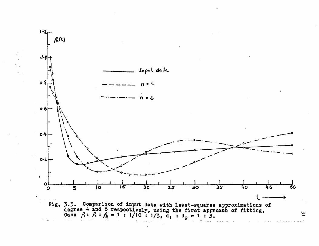
3.3. Comparison of input data "Yri th least-squares

approximations of degree 4 and 6

respectively, using the first approach

of fitting ................. ~ ............ 31

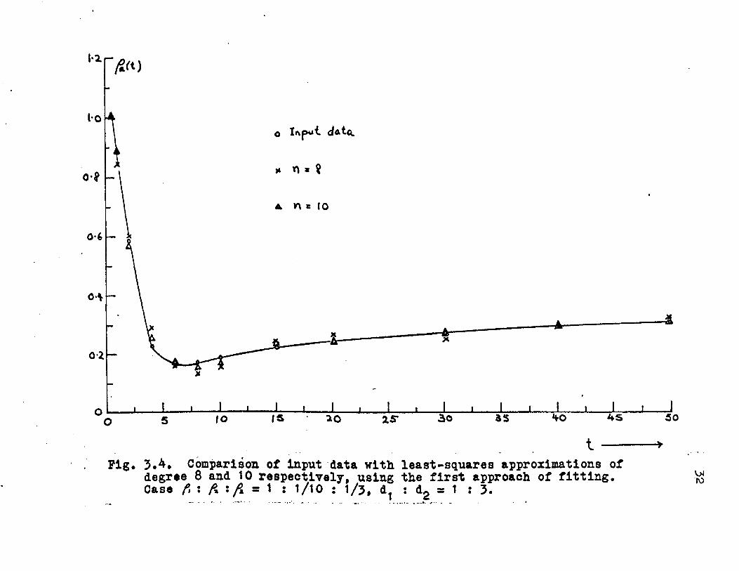
3.4. Comparison of input data with least-squares


respectively, using the first approach

of fitting .............................. 32

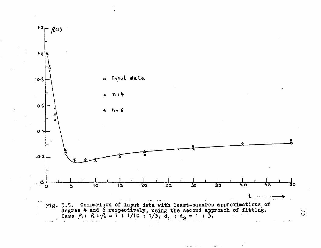
3.5. Comparison of input data with least-squares


respectively, using the second approach

of fitting. . . . . . . . . . . . . . . . . . . . . . . . . . . . . . 33

3.6. Apparent resistivity obtained by direct .

computation from least-squares polynomial

using an interval At = 0.05 and by

interpolation between values generated

ix

at an interval A t = 0. 5 • • • • • • • • • • • • • • • • • 37

3.7. Apparent resistivity curves for two-layer

case, logarithmic plotting •.•••.••••••••• 40

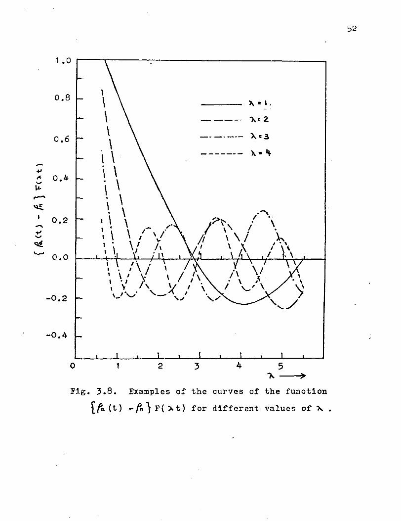
3.8. Examples of the curves of the function

{ fa (t) - fn} F ( 7-. t) for different

values of~ •••••••••••.•.••••••••••••••• 52

3.9. Kernel obtained by numerical integration and

3.1 o.

3. 11 •

3.12.

3.13.

from theoretical formula. Case f. : R: fs: f't

- 1:1/3:3:1/10, d1 :d2:d3 = 1 :4:1 ••••••••• 55

Kernel obtained by numerical integration and

from theoretical formula. Case f. : ({: f. : F~ - 1:1/3:3:1/10, d1 :d2:d3 = 1 :3:2 ••••••••• 56


from theoretical formula. Case f. : f.,_: ~: f'+

= 1 : 1 /3 : 3: 1 I 1 o, d 1 : d2 : d3 = 1 : 2: 3. • • • • • • • • 57


from theoretical formula. Case f. : R: fs: f...

= 1:1/3:3:1/10, d1 :d2:d3 = 1:1 :4 ••••••••• 58

Examples of the curves of the function

{ fa ( t ) - fn} J 0 ( .i\ t ) for different

values of A . . . . . . . . . . . . . . . . . . . . . . . . . . . . 66

3.14 Associated kernel obtained by numerical

3.15.

integration and from theoretical

formula. Case R: fa: f,: f~ = 1:1/3:3:1/10,

d1 :d2:d3 = 1 :4:1 •••.••••••••••••••...•••• 71

Associated kernel obtained by numerical


3. 16.

3.17.

X

formula • Case ~ : ({ : ~ : fct- = 1 : 1 13 : 3 : 1 I 1 0 ,

d1 :d2:d3 = 1 :3:2 ••.•••.••.•••..•••.•••••• 72



formula • Case R : R : fi : f't = 1 : 1 13 : 3 : 1 I 1 0,

d1 :d2:d3 = 1 :2:3 ••••••.•...•••••••••••••• 73



formula. Case f.: R: B: f'+ = 1 :1/3:3:1/10,

d 1 : d2 : d3 = 1 : 1 :4. • . . • • • • • • • • • • • • . • • . • • • • • 7 4

4.1. Curves of two-layer kernels with positive

reflection factor ••••..•••••••••••••••••• 86

4.2. Curves of two-layer kernels with negative

reflection factors •••••.••••••••.•••••••• 87

4.3. Relation between K1 (~)and T1 ••••••••••••••••• 88

4.4. Log I T1

I vs. A • Analysis of two-layer

kernels •.............................. · • • 95

4.5. Master diagram of the asymptotic straight

line log Y = -,... d log e • • • • • • • • • • • • • • • • • • 96

4.6. Classification of three-layer apparent

resistivity curves according to their

characteristic shapes ••••••.•..••.••••••• 97

4.7. Curves of three-layer kernels for the case

f. : ~ : f.J = 1 : 1 o : 1 11 o ~ • • . . . . • . . . • . . . . • . • . 98


R : f2. : f& = 1 : 1 11 o: 1 o. • . . . . . . . . . . . . . . • . . . 99

xi


4.1 o.

4. 11 •

4.12.

4.13.

4. 14.

4. 15.

4. 16.

4.17.

4.18.

4.19.

4.20.

P. : fa. : f'3 = 1 : 3 : 1 0 • • • • • • • • • • • • • • • • • • • • • • • 1 00

Curves of three-layer kernels for the case

P. : {{ : ~ = 1 : 1 /3: 1 11 0. • • • • • • . • • • • . • • • • • • 1 01

Analysis of three-layer kernel of the case

R : Pa : 6 = 1 : 1 o : 1 I 1 o, d 1 : d2= 1 : 4 • • • • • • • • 1 o2


f.: fa.:~ = 1 :10:1110, d1 :d2= 1 :1t ••••••• 103


fr : R : fi = 1 : 1 o: 1 I 1 o, d 1 : d 2= 1 : 213. • • • • • 1 o4


P. : R : fa. = 1 : 1 o : 1 I 1 o , d 1 : d2 = 1 : 1 I 4. • • • • 1 05

The function T 1 and its related three-layer

kernel. Case f.: ({: f3 - 1 :10:1110,

d1 :d2 = 1 :114 ••.•.•.•.•.•.••••••••••••••• 106

The function T1 and its related three-layer

kernel. Case P.: fi: B _ 1:1110:10,

d1 :d2 = 1 :114 •••••.••.•••••••...•...•.••• 107

Curves of two-layer associated kernels with

positive reflection factors ••••••••.••••• 115

Curves of two-layer associated kernels with

negative reflection factors ••.•••••.••••• 116

Analysis of two-layer associated kernels

with positive reflec~ion factors •••••.••• 117

Analysis of two-layer associated kernels

with negative reflection factors ••••••••• 118

4. 21 •

4.22.

4.23.

4.24.

4.25.

4.26.

4.27.

4.28.

4.29.

4.30.

4.31.

xii

General relation between the associated kernel

and the function Q1 ••••••.••••••••••••••• 122

The function Q1 and its related two-layer

associated kernel. Case k 12=1 .o .......•.. 123

The function Q1 and its related two-layer

associated kernel. Case k12=-0.8 •••••.••• 124

Curves of three-layer associated kernels for

the case f, : ~ : ~ = 1 :1 0:1/1 o ••••. 0 • • • • • • 125


the case f.:~:~= 1 :1/10:10 •••••••..••. 126


the case f.: R: f3 = 1 :3:10 ••••••••••••••• 127


the case f. : R : ~ = 1 : 1 /3 : 1 /1 0. • • • • • • • • • • 1 28

Analysis of three-layer associated kernel of

thecase f.:({:~=1:10:1/10,

d 1 : d2 = 1 :4 •.•.••.. 0 ••• 0 • • • • • • • • • • • • • • • • • 1 29


the case f.:({: f.s = 1 :10:1/10,

d : d = 1 : 1 i . . . . . . . . . . . . . . . . . . . . . . . . . . . . . 1 30 1 2


the case f. : R: ~ = 1 : 1 0: 1/1 0, ~ ... _ ..

d1 :d2 = 1 :2/3 ••••••••••••••••••••••••.••• 131


the case A : f~: ~ = 1 :10:1/1 o,

d 1 : d2 = 1 : 1 14. • • • • • • • • • • • • • • • . • • • • • • • • • • • 1 32

4.32.

4.33.

4.34.

4.35.

4.36.

x111

1.Caster set of two-layer kernel curves for

cases with different reflection factors,

logari tl:unic plotting... • • . . . . • . . . . • • • • • • • 138

¥~ster set of two-layer kernel curves for

cases with different reflection factors,

logarithmic plotting •••••••..•••••••••••• 139

Decomposition of a three-layer kernel by

the method of logarithmic curve-matching,

case f.:{{:~= 1:10:1/10, d1 :d2= 1 :4 •••• 140

Decomposition of a four-layer kernel by the

method of logarithmic curve-matching,

Case f,: f:a.: f3: R. = 1:1/3:3:1/10,

d1 :d2:d3 = 1 :3:2 •••••.•••.••••••••••••••• 141

Decomposition of a four-layer kernel by the

method of logarithmic curve-matching,

Case f.:({:({: f,. = 1:10:3:1,

d 1 : d2 : d 3 = 1 : 2 : 3. • • • • • • • • . • • • • • • • • • . • • • • • 142

A.1. Point current electrode on surface of

homogeneous earth ••••••••••••••••••••.••• 155

A.2. A general four-electrode configuration •••••.•• 155

A.3. The Wenner configuration •••••••••••••••••••••• 155

C.1. Graph of the function

00 1 F(x) = L ' ~ ' ••••••••••• 172

kzo

F.1. Examples of the curves of kernel of four-layer

earth •• •••.....•...•••...•.....•........• 1 82

xiv

F.2. Analysis of a four-layer kernel by numerical-

graphical method. Case f, : fi : ~ : P,.. =

1:113:3:1110, d1 :d2:d3 = 1:4:1 ••••••••••• 183


graphical method. Case f! : P~: f., : ~ =

1 : 1 13:3 : 1 11 o, d 1 : d2 : d3 = 1 : 3 : 2. • • • • . • • • • • 1 84


graphical method. Case f.: R: ({: R =

1 : 1 13 :3 : 1 11 o, d 1 : d2 : d3 = 1 :2 :3. • • • • • • • • • • 1 85


graphical method. Case f. : R : ~ : f:. =

1 : 1 13 :3 : 1 11 o, d 1 : d2 : d3 = 1 : 1 :4. • • • • • • . • • • 1 86

F.6. Examples of the curves of associated kernel

of four-layer earth. • • • • • • • • . • • • • • • • • • • • • • 1 87

F.7. Analysis of a four-layer associated kernel by

numerical-graphical method. Case

1 : 4: 1 • • • • • • • • • • • • • • • • • • • • • • • • • • • • • • • • • • • • 1 88



1 : 3 : 2 • • • • • • • • • • • • • • • • • • • • • • • • • • • • • • • • • • • • 1 89



P. : R : 6 : p,.. = 1 : 1 /3 :3 : 1 I 1 o, d 1 : d 2 : d 3 =

1 : 2 : 3. . . . . . . . . . . . . . . . . . . . . . . . . . . . . . . . . . . . 1 90

F. 1 O. AnalyGis of a four-layer associated kernel by


XV

1:1:4 •••••.•.•••••.•••....•.......•.•.••• 191

xvi

LIST OF TABLES

TABLE PAGE

3.1. Example of the fitting of the curve fa. (t)

vs. t by least-squares approximations

of different degrees..... • • . . . . . . . • • . • . • • 34

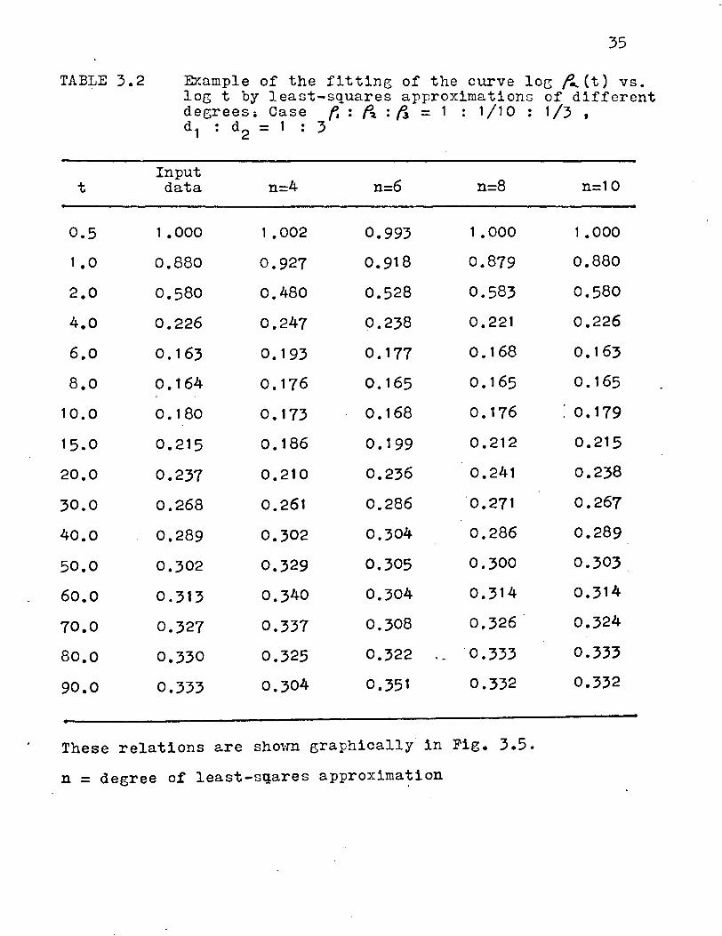
3.2. Example of the fitting of the curve log ~(t)

vs. log t by least-squares approximations

of different degrees ••••••.••.••..••••••• 35

3.3. Values of fa(t) generated by least-squares

3.4.

approximation of degree 10 ••••••••••••••• 36

An example of the numerical values of K11 (J'..) 1

obtained by the method of composite

rule. . . . . . . . . . . . . . . . . . . . . . . . . . . . . . . . . . . . • 53

3.5. Numerical values of the kernel obtained by

integration of apparent resistivity

data and from theoretical formula •••••••• 59

3.6. Numerical values of the kernel obtained by

integration of apparent resistivity

data and from theoretical formula •••••••• 60

An example of the numerical values of B11 (X) 1

obtained by the method of partial

approximation of the integrand by a

parabolic arc. • • • • • • • • . • • • • • • • • • . • . • • • . • • 67

3.8. Numerical values of the ass'ociated kernel

obtained by integration of apparent

resistivity data and from theoretical

formula. . . . • • . . . . . . . . . . . . . . . . . . . . . • • . • • • . 75

3.9. Numerical values of the associated kernel

obtained by integration of apparent

resistivity data and from theoretical

xvii

formula • .•............................... 76

4.1. Comparison of a two-layer kernel with tw·o

three-layer kernels associated with

the case of thin intermediate layer •••••• 146

CHAPTER I

INTRODUCTION

1

One of the most popular techniques ln shallow geophysi

cal exploration is the use of d. c. (d. c. = direct current)

resistivity depth soundings. In such measurements the resls-

tivity of the earth is studied with an array of four

electrode contacts, two of which are used to supply a current

to the ground, and two of which are used to detect the electric

field established in the ground by the current. A widely used

electrode array is the Wenner system, the description of which

can be found in Appendix A. By assumlng the materials beneath

the surface of the ground to be uniform, values of apparent

resistivity are calculated from the measurements. The concept

of apparent resistivity (see Appendix A for definition) per

mits the use of very simple mathematical formulas expressing

the relationships between voltage, current, electrode spaclng

and the resistivity of the supposedly uniform earth. If the

ground is not uniform, but consists of a series of strata in

which the electrical properties within each stratum are uni

form, then the variation of resistivity with depth in the

ground may be studied by making apparent resistivity deter

minations with an increasing sequence of separations between

the electrodes. Generally speaking the larger the electrode

spacing the more the observed data will reflect the resis

tivity of layers at depth in the earth.

2

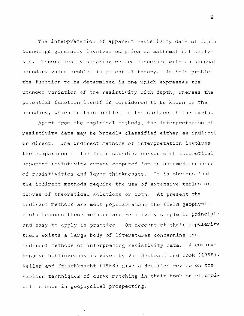
The interpretation of apparent resistivity data of depth

soundings generally involves complicated mathematical analy

SlS. Theoretically speaking we are concerned with an unusual

boundary value problem in potential theory. In this problem

the function to be determined is one which expresses the

unknown variation of the resistivity with depth, whereas the

potential function itself is considered to be known on the

boundary, which 1n this problem is the surface of the earth.

Apart from the empirical methods, the interpretation of

resistivity data may be broadly classified either as indirect

or direct. The indirect methods of interpretation involves

the comparison of the field sounding curves with theoretical

apparent resistivity curves computed for an assumed sequence

of re~istivities and layer thicknesses. It is obvious that

the indirect methods require the use of extensive tables or

curves of theoretical solutions or both. At present the

indirect methods are most popular among the field geophysi

cists because these methods are relatively simple in principle

and easy to apply in practice. On account of their popularity

there exists a large body of literatures concerning the

indirect methods of interpreting resistivity data. A compre

hensive bibliography is given by Van Nostrand and Cook (1966).

Keller and Frischknacht (1966) give a detailed review on the

various techniques of curve matching in their book on electri

cal methods in geophysical prospecting.

3

In the direct methods of interpretation no assumptions

about the layer resistivities and thicknesses are necessary,

but some geometric limitations are generally imposed on the

earth model used. The general procedure of the direct

methods of interpretation involves two main steps: (l) the

calculation of a function which is termed the Slichter's

kernel from the observed apparent resistivity data, and

(2) the determination of the layer resistivities and thick

nesses from the resulting Slichter's kernel. From the

theoretical point of view the direct approach is equi~alent

to the search for a solution of the integral equation relat

ing the apparent resistivity to the true resistivity and

thickness of each of the individual layers composing the earth.

The direct methods of interpretation have first been

studied in a series of papers by Langer (1933), Slichter

(1933), and Stevenson (1934) respectively for the case of a

continuous vertical variation of resistivity. In these

papers it lS assumed that the resistivity p(z) can be

expressed as a power series in z (the depth); the coefficients

of this power series are determined by comparison with the

coefficients of another power series representing the

Slichter's kernel. The Slichter's kernel must be determined

from the field data, namely the electric potentials, through

integration. The methods of calculation are extremely cumber-

some because of the highly complicated algebraic relations

relating the coefficients of the two power series. There

is still another serlous drawback in these methods. If a

discontinuity in resistivity exists, the power series

representations of both the resistivity function and the

Slichter's kernel break down. In practice it lS found that

the function which best approximates the true resistivity

variation in layered earth is a stepwise function of depth.

Accordingly the methods developed by these earlier investi

gators have hardly found any application to practical pro

blems.

4

Pekeris (1940) devised a numerical-graphical method for

the analysis of the Slichter's kernel. His method works

quite well but subjects to the restriction of small depth

values. Later Vozoff (1956) proposed another method for

analyzing the kernel. Vozoff's method involves the fitting

of a kernel integrated from potential field data with a

theoretical kernel calculated from an assumed sequence of

layer resistivities and thicknesses. In the process of

fitting which is carried out automatically on a digital

computer the parameters of the kernel, namely the resistivity

and thickness, are changed slowly until a good fit is obtained

between the field and theoretical kernels. It must be pointed

out that in both the papers by Pekeris and Vozoff respectively

the actual computation of the kernel from the field data is

not discussed.

In all the papers mentioned above none of these writers

shows how the kernel may be calculated from the apparent

5

resistivity data. All these earlier methods requ1re a

knowledge of the electric potentials along the measuring

line on the ground surface. But this knowledge is not

obtained by the field procedures that are commonly used now

adays. This may be another reason why these methods are

never adopted by the field geophysicists.

The most recent study on the direct methods of interpre

tation is presented by Koefoed 1n a series of two papers

(1965 and 1966). In his first paper Koefoed derived an

explicit integral expression for the Slichter's kernel 1n

terms of the apparent resistivity function as measured by the

Schlumberger electrode system. Then he proceeded to show how

the integral expression of the kernel could be evaluated by

approximating the apparent resistivity function with either a

set of unrational algebraic functions or a set of exponential

functions. In his second paper Koefoed dealt with the Wenner

electrode system in a similar manner, but he did not obtain

any explicit expression for the kernel in terms of the apparent

resistivity function. The derivation of such an express1on

was later achieved by Paul (1968). Although the formulas

derived by Koefoed are not very complicated from the computa

tional point of view it is rather disappointing that he did

not show how his formulas could actua~ly be applied to practi

cal situations.

Review of the literatures shows that the maJor obstacle

which prevents the practical application of the direct methods

6

of interpretation has been that no suitable formulas are

available to enable one to compute the Slichter's kernel or

related functions directly from the apparent resistivity data.

It was one of the main objectives of this thesis to develop

a technique for deriving from the apparent resistivity data

measured by the Wenner electrode system some functions from

which the layer resistivities and thicknesses might be deter-

mined. Another objective was to devise methods for the

analysis of the resulting functions derived from the field

data.

In the following the solution of the boundary value

problem associated with an n-layered earth model is first

discussed in Chapter II. In the same chapter the solution

for the integral equation resulting from solving the boundary

value problem is also discussed. It will be shown that the

process of solving the integral equation leads to two func-

tions which will be designated as the 'kernel' and the

'associated kernel' respectively. As will be explained later

the kernel defined ln this thesis lS not identical with the

Slichter's kernel. Numerical techniques for computing the

kernel and the associated kernel are derived in Chapter III.

Finally the methods for determining the layer resistivities

and thicknesses from the kernel functions are presented in

Chapter IV.

CHAPTER II

THEORETICAL EARTH MODEL FOR THE INTERPRETATION OF APPARENT RESISTIVITY DATA

Basic Equations for Direct Current

7

The flow of direct current 1n a conducting medium 1s

governed by the Ohm's law:

-+ -+ J = oE ( 2. 1)

-+ where J 2 = current density measured 1n amp/m ,

E = electric field intensity measured in volts/m,

o = conductivity of the medium in mho/m.

It 1s sometimes more convenient to write (2.1) 1n the form

-+ -+ J = E/p ( 2 • 2)

where o = 1/p, p being the resistivity expressed 1n ohm-m.

In addition to Ohm's law the current density has to satisfy

the divergence condition:

-+ 'V. J = 0 ( 2 • 3)

This divergence condition must be satisfied everywhere in a

source-free region.

Since stationary electric fields are conservative, that -+ -+

1s 'V x E = 0, E may be derivable from a scalar potential

function V as follows:

-+ E = -'VV ( 2. 4)

where V is measured in volts. By substituting (2.4) into

(2.1) we get

8

-+ J = -o VV = 1 vv

p ( 2 . 5 )

It follows from (2.5) and (2.3) that

V.(-oVV) = 0

and hence

( 2 • 6)

If the conductivity o remains constant throughout the entire

medium, then

( 2 • 7)

which is the well known Laplace's equation. So the potential

ln this case lS a harmonic function.

Suppose that the medium is divided into two reglons of

different conductivities, but within each region the conduc-

tivity is a constant. Let pl and p 2 be the resistivities of

these two regions respectively. The potential in each region

is still a harmonic function, but at the interface between

the two regions two conditions must be satisfied: ( i) the

potential V must be continuous across the boundary, and -+

Cii) the normal component of the current density J must also

be continuous. The first condition is equivalent to the fact

that the amount of work required to deposit a given charge on

one side of the boundary should not differ from that required

to deposit the same charge on the other side. The second

condition is a consequence of the requirement that the current

is conserved - all the current entering the boundary plane

9

from one side must leave it from the other side. From the -+ -+

conditions V.J = 0 and VxE = 0 one can formally deduce that

these two boundary conditions can be expressed mathematically

by the following equations:

( 2 . 8)

for the continuity of the potential V, and

( 2 . 9)

for the continuity of the normal component of the current -+

density J. In (2.9) n lS the unit vector normal to the

interface. With the use of (2.5) we can write (2.9) as

(2.10)

Solution of Boundary Value Problem

In the interpretation of resistivity data of depth

soundings it is customary assumed that the ground is made

up of two or more horizontal layers, each of which has a

constant resistivity and finite thickness except the bottom-

most layer being theoretically assumed to extend to infinity.

Practical experiences show that such a model of the earth can

often be used to approximate very closely the subsurface

physical and geological conditions. From the theoretical

point of view this model has the advantage that the mathema

tical theory involved in.the analysis of the problem is not

too complicated to handle.

10

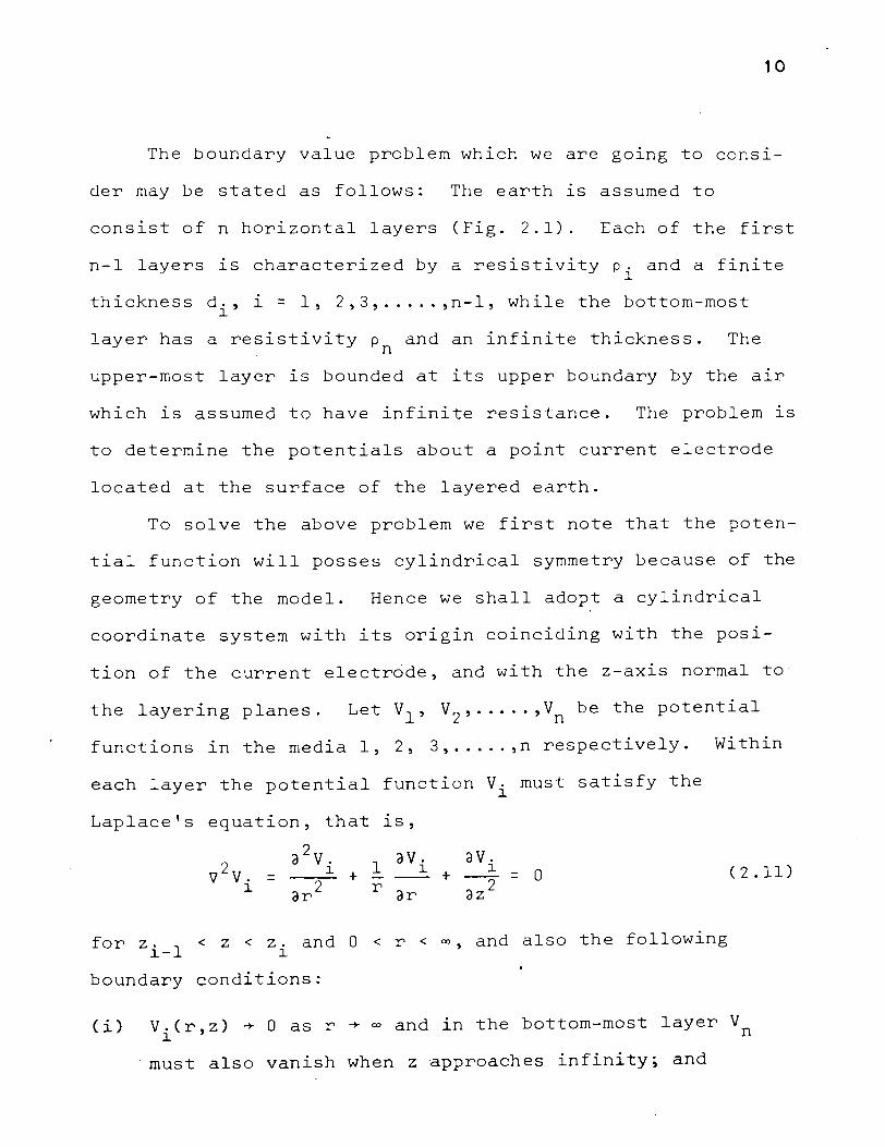
The boundary value problem which we are going to consi-

der may be stated as follows: The earth lS assumed to

consist of n horizontal layers (Fig. 2.1). Each of the first

n-1 layers lS characterized by a resistivity p. and a finite l

thickness d., i = l, 2,3, ..... ,n-1, while the bottom-most l

layer has a resistivity p and an infinite thickness. The n

upper-most layer lS bounded at its upper boundary by the air

which is assumed to have infinite resistance. The problem is

to determine the potentials about a point current electrode

located at the surface of the layered earth.

To solve the above problem we first note that the poten-

tial function will posses cylindrical symmetry because of the

geometry of the model. Hence we shall adopt a cylindrical

coordinate system with its origin coinciding with the posi-

tion of the current electrode, and with the z-axis normal to

the layering planes. Let V1 , V2 , ..... ,Vn be the potential

functions in the media 1, 2, 3, ..... ,n respectively.

each layer the potential function Vi must satisfy the

Laplace's equation, that 1s,

a2

v. 1 avi --~l~ + ar 2 r ar

= av.

+ l = 0 az 2

Within

(2.11)

for z. 1

< z < z. and 0 < r < oo, and also the following l- l

boundary conditions:

(i) V.(r,z) ~ 0 as r ~ oo and in the bottom-most layer V 1 n

must also vanish when z approaches infinity; and

11

Point current electrode located on the ground sur .face

/! "00 o/ ~r Zo

l 1 f. d,

t z, I

fa d ..

%= !

~ =:"'\ - ' I z ... .~

I t f!.-~ cl"_"

t . t z •. t

f,. .• d •••

z .... ! ~ d ..

'~ ! z DQ

Fig. 2.1. n-layer earth model

( i i)

and

at the interface z. between layer 1 Qnd layer i+l l

av. l

az z = z. l

= l

pi+l

d v. l l+ dZ z = z.

l

12

In addition to the above conditions the potential function v1

1n the first layer has to satisfy two further conditions:

Ci) s1nce no current can flow across the boundary the normal

component of the current density must vanish at z = 0.

This implies that

= 0 z = 0

and Cii) v1

must approach the correct express1on for the

potential about a single point source in a uniform

medium, that 1s,

as R -+ 0 '

where R 2 2 k = (r + z ) 2

•

The solution of Laplace's equation can be achieved by

the method of separation of variables. The procedure of

solving the problem is outlined in Appendix B. \-Je shall only

state here the final form of the solution.

13

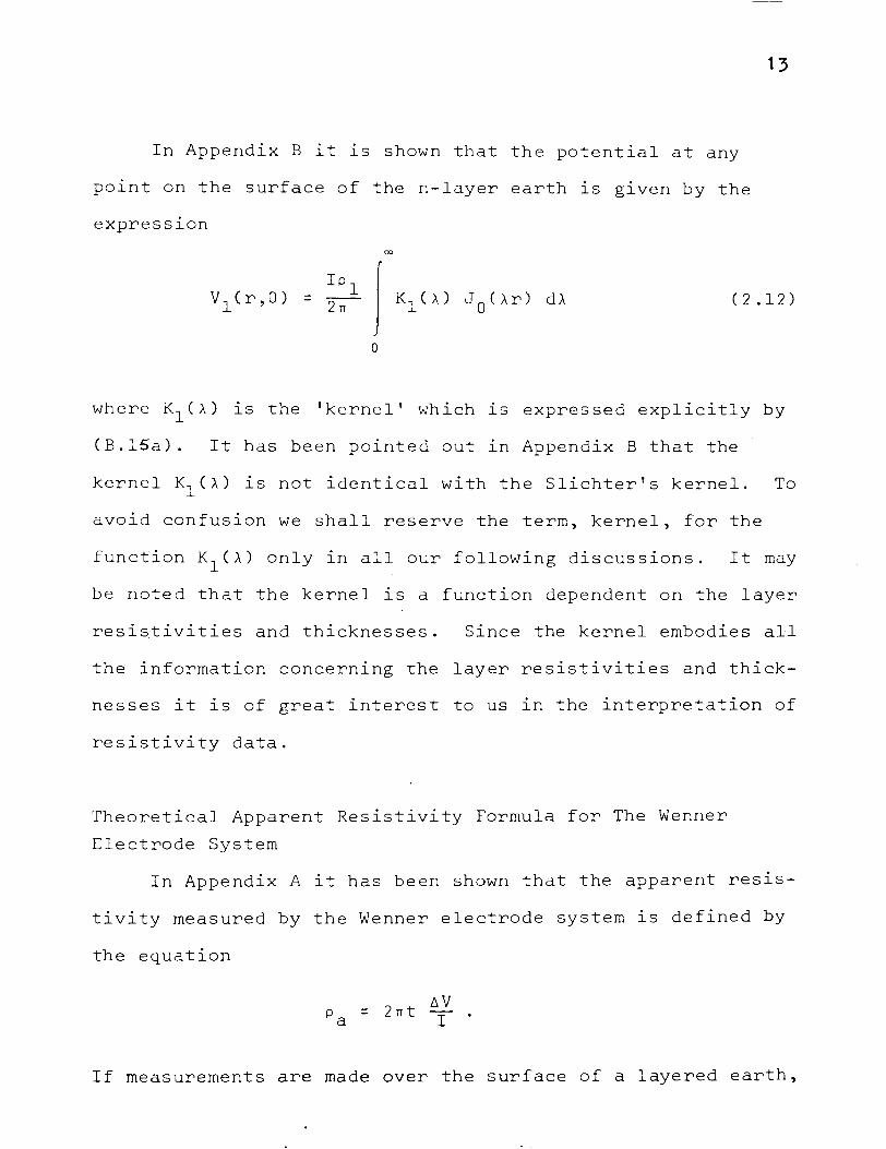
In Appendix B it is shown that the potential at any

point on the surface of the n-layer earth is given by the

express1on

00

=~I 2n (2.12)

0

where K1 (A) lS the 'kernel' which lS expressed explicitly by

(B.l5a). It has been pointed out 1n Appendix B that the

kernel K1 (A) 1s not identical with the Slichter's kernel. To

avoid confusion we shall reserve the term, kernel, for the

function K1 (A) only in all our following discussions. It may

be noted that the kernel is a function dependent on the layer

resistivities and thicknesses. Since the kernel embodies all

the information concerning the layer resistivities and thick-

nesses it is of great interest to us in the interpretation of

resistivity data.

Theoretical Apparent Resistivity Formula for The Wenner

Electrode System

In Appendix A it has been shown that the apparent res1s-

tivity measured by the Wenner electrode system is defined by

the equation

If measurements are made over the surface of a layered earth,

14

then by making use of (2.12) one can easily show that the

potential difference 6V is given by the following expression:

6V = dA. TI

It follows that the theoretical apparent resistivity function

for an n-layer earth is given by

pa(t) = 2tpl JooKl(A) !J0

CAt) - J0

(2At)} dA •

0

(2.13)

Equation (2.13) forms the basis of the curve-matching

methods of interpreting resistivity data obtained by using

the Wenner electrode system. By assigning hypothetical

vaiues to the layer resistivities and thicknesses one can

compute theoretical apparent resistivity curves from (2.13).

Mooney and Wetzel (1956), for example, have prepared a set

of about 2300 curves for the Wenner electrode system for one,

two, and three layers over an infinite substratum. These

curves are commonly employed for curve-matching purpose.

In practice the apparent resistivity function p (t) lS a a

known function determined by direct field measurements while

the kernel K1 (A.) appearing under the integral sign of (2.13)

is an unknown function because the layer resistivities and

thicknesses cannot be determined by direct observations.

Thus (2.13) lS essentially an integral equation. The

15

interpretation of the resistivity data amounts to the search

for a suitable solution for this integral equation.

Solution of Integral Equation

A solution of the integral Equation (2.13) can be

obtained by making use of the Hankel inversion theorem

(Sneddon, 1951) which may be stated as follows: The Hankel

transform of a function f(x) is defined by

roo H(u) = J xf(x)J ~(ux) dx

0

which exists if f(x) lS piecewise continuous ln any finite

interval and absolutely integrable. If, in addition, f(x)

possesses piecewise continuous derivative in any finite

interval the inversion integral

exists.

~ {f(x+O) + f(x-0)} = J~ uH(u)J"(ux)

0

If f(x) lS continuous at the point x, then

f(x+O) = f(x-0) = f(x)

so that the theorem gives

f(x) = J~uH(u)J 0 (ux) du.

0

du

16

In the special case w = 0 we have the Hankel transform palr,

H(u) = J~xf(x)J 0 (ux) dx (2.14a)

0

f(x) = J~uH(u)J 0 (ux) du. (2.14b)

0

To solve the integral Equation (2.13) we may proceed as

follows: if both sides of (2.13) are multiplied by J0(A't)

and then integrated with respect to t from 0 to oo we have

0 0 0

0 0

The application of the Hankel transform palr (2.14a) and

(2.14b) to the right hand side of the above equation leads to

dt (2.15)

0

which lS the desired solution of the integral equation. How-

ever, (2.15) is not an explicit expression for the kernel

K1 (A). To derive such an expression we proceed in the

17

following manner. By setting A equal to A, A/2, A/4,

A/8, .......... , A!2n ....... and then multiplying the result-

ing equations by l, l/2, l/4, l/8, .......... , l/2n, ...... .

respectively, we obtain the following set of equations:

= 1 Joopa(t) K1 CA) - 112 K1 CA/2) A

2P

1 J 0 CAt) dt

0 (2.16)

A/4 dt

0

100 p ( t)

= A/16 ~Pl dt

0 . . . . . . . . . . . . . . . . . . . . . . . . . . . . . . . . . . . . . . . . . . . . . .

0 . . . . . . . . . . . . . . . . . . . . . . . . . . . . . . . . . . . . . . . . . . . . . . Summing up both sides of the above equations we obtain

<X>

r~ Pa (t) L:

A J0

(At/2n) = n=O 2 2n pl

dt

0

By interchanging the order of summation and integration for-

mally we have

18

rpa(t) 00

Kl(:>.) :>.

{ 1 Jo(>-t/2n)} = 2 I 2 2n dt

pl n=O (2.17)

0

By letting

00

F(:>.t) I 1 Jo(>-t/2n) =

2 2n n=O (2.18)

(2.17) can be written as

Kl(>..) >.. rpa(t) F(>..t) dt = 2pl

(2.19)

0

which is the desired expresslon for the kernel.

The infinite series (2.18) can be shown to converge

uniformly and it behaves almost like the Bessel function

J 0 (>..t). A brief discussion of the properties of F(>..t) is

given in Appendix C.

Though (2.15) is not an explicit expresslon for the ker-

nel it serves to define a useful function from which one may

determine the layer resistivities and thicknesses. By letting

(2.20)

(2.15) can be written as

dt. (2.21)

0

For the ease of description we shall define B1 CA) as the

'associated kernel' for n-layer earth.

19

In conclusion we note that if the apparent resistivity

function p (t) is determined from field observations then a

(2.19) and (2.21) will enable us to compute the kernel and

the associated kernel respectively from the observed resis-

tivity data. Once the kernel and the associated kernel

are known the layer resistivities and thicknesses may be

obtained from these functions by some suitable methods of

analysis. In Chapter III we shall consider the calculation

of the kernel and the associated kernel from the observed

apparent resistivity data. This is followed by the deriva-

tion of the methods used for analyzing K1 CA) and B1 CA) in

Chapter IV.

CHAPTER III

NUMERICAL METHODS FOR CALCULATING THE KERNEL AND THE ASSOCIATED KERNEL

20

In Chapter II it has been shown that the solution of the

integral equation for the Wenner electrode system leads to

the following results:

K1

(A) A!2 J~pa(t)

F(At) dt = pl

0

and

B1

(A) Al2 J~pa{t)

J 0 <At) dt = pl

0

where K1 (A) and B1 (A) are the kernel and the associated ker-

nel respectively. The apparent resistivity function p (t) a

which appears in the integrands of both the above integrals

is, in practice, only known empirically from a finite number

of measurements, but not known analytically. Consequently

K1 (A) and B1 (A) cannot be determined by any method of direct

integration. In order to obtain K1 (A) and B1 (A) from the

observed apparent resistivity data one has to resort to the

numerical techniques of integration. In this chapter we are

going to develop the methods for evaluating the kernel and

the associated kernel numerically.

21

Least-Squares Approximation of Apparent Resistivity Data

In the above introductory remarks we point out that the

apparent resistivity is observed only at certain number of

electrode spacings. For numerical evaluation of the inte-

grals of K1 CA) and B1 CA) respectively, however, one needs to

know the values of p (t) at a large number of points along a

the t-axis; the set of field data is obviously inadequate for

such purpose. Of course, it is highly impracticable and

uneconomical to make a very large number of measurements ln

the field. The practical remedy to the problem is to inter-

palate the unknown values of p (t) from the observed data. a

The interpolation can be achieved by approximating p (t) with a

some suitable function. Since the field data usually contain

a certain amount of noise the appropriate technique of approx-

imation to be used would be the least-squares method.

The least-squares techniques of approximating function

are well known and are described in many standard texts of

numerical analysis (e.g. Hildebrand, 1956; Ralston, 1965).

In the following we shall consider those facts which are

pertinent to our problem.

Outline of least-squares method. Suppose that the

values of the apparent resistivity function p (t) lS observed a

at a sequence of data points, namely {ti}' i = 1, 2, ..... n.

These observed values of p (t) will generally be in error. a

Let p (t.) denote the true value of pa(t) at t. and p (t.) a l l a l

the observed value also at t .. l

Next suppose that we have a

22

. set of polynomials {P.(t)}, j being the degree of the poly

]

nomials and j = 0, 1, 2, ..... , m, which are orthogonal over

the set of points {t.}. l

Our objective is to approximate

P (t.) by a linear combination of {P.(t)}, that is, a l J

- (t.) -P a l

m l:

J=O c. p.(t.)

J J l for l = 1,2, ..... ,n ( 3. 1)

According to the principle of least-squares the coefficients

c.'s must be determined in such a way that the function J

n l:

i=l {p (t.) -

a l

m l:

j=O

2 c.P.(t.)} J J l

( 3 . 2 )

lS minimized. If H lS mlnlmum, then at the point ln question

n m = 2 l: {p (t.)- l: c.P.(t.)} (-Pk(ti)) = 0

i=l a l j=O J J l

or

m n n l: c. l: P.(t.)Pk(t.) =

j=O J i=l J l l l: p ( t . ) Pk ( t . )

a l l i=l ( 3 . 3)

fork= 0, 1, 2, 3, ..... , m. The system (3.3) consists of

m+l linear equations for m+l unknown c.'s. This system lS J

called the normal equations. If the determinant of the

coefficients does not vanish we can solve for the

By making use of the orthogonal relation

C • IS, J

n l: p . ( t . ) pk ( t . ) = 0

i=l J l l for J = k

we find that the solution of (3.3) ls glven by

n E p ( t . ) Pk ( t . )

i=l a l l

23

n 2 ( 3 . 4)

E {Pk(ti)} i=l

A few words may be said about the selection of m, the

degree of polynomial approximation, for a given value of n.

One way of making the choice is to compute the function

where

02 = E 2

I (n - m - 1) m m

n E

i=l {p (t.) -

a l

m E

j=O

2 c.P.(t.)} J J l

( 3. 5)

According to the statistical null hypothesis (Ralston, p. 234)

h f 2. · f f M Ml t e expected value o 0 lS lndependent o m or m = , + , m

..... , n-1. In practice, since we do not know M, we would

wish to solve the normal Equations (3.3) form= 1, 2, 3, ...

2 d . 1 2 d . 'f' and compute 0 an contlnue as ong as 0 ecreases slgnl l-m m

cantly with increasing m. As soon as a value of m lS reached

after which there is no significant change in 02 then this m

value is that of the null hypothesis, and we have the desired

least-squares approximation.

24

In the above discussion it 1s pointed out that the

search for a suitable m would require one to solve the normal

Equations (3.3) repeatedly. This is indeed a very tedious

process. However, such a computational problem does not

arise with the use of orthogonal polynomials since all the

coefficients ck can be calculated independently from (3.4).

It may also be noted that the use of orthogonal polynomials

avoids the problem of forming an ill-conditioned matrix of

the coefficients in (3.3) when large values of mare used.

Generation of orthogonal polynomials. The set of

orthogonal polynomials {P.(t)} which is used in the least]

squares approximation may be generated in a number of ways.

The writer finds that a method proposed by Forsythe (1957)

is most suited for his purpose. Forsythe's method of gener-

ating orthogonal polynomials may be outlined as follows.

Suppose that {Pj(t)} 1s any sequence of polynomials

satisfying the orthogonal relationship

n E

i=l p . ( t . ) pk ( t . ) = 0

J l l for J -f k

with respect to a sequence of data point {ti}' i = 1, 2,

3, ..... , n. This sequence of orthogonal polynomials can be

generated by the following recursion formulas:

25

p . ( t) = 0 -]

PoCt) = l

pl(t) = (t pl) PoCt) ( 3 . 6)

P 2 Ct) = (t p2) P1 Ct) - ql P0

Ct)

where p and q are constants so chosen to make the orthogo-m m

nal relations hold. It can be shown that

n 2 I t. {P

1Ct.)}

i=l l m- l

Pm = n 2 I {P

2Ct.)}

i=l m- l

( 3 . 7)

and

n I t. p l(t.) p 2(t.)

i=l l m- l m- l

qm = n 2 I p 2(t.)

i=l m- l

( 3. 8)

The range of the independent variable t may be normalized for

range 0 < t! < l by using the transformation l

( 3. 9)

Some computational details. The Forsythe's method of

generating orthogonal polynomials for data-fitting is well

suited for cases in which the data points are not equally

spaced. Also the computational works involved in this method

26

can be performed automatically by a digital computer. All

the results presented in the following were computed by the

IBM-360 MOD 50 system at the UMR computer center. Outline of

the computational procedures lS given in Appendix E.

It may be pointed out that our prlmary aim here is to

obtain a single least-squares approximating function that can

fit the apparent resistivity data in the entire range of

electrode spacing concerned.

Two different approaches have been tried to fit the

apparent resistivity data by the least-squares method out-

lined above. The first method consists of the fitting of

the curve p (t) vs. t, while in the second method attempt lS a

made to fit the curve log p (t) vs. log t. a The use of the

second method is due to the following reasons. In practice

a typical sequence of electrode spacing used for field measure-

ments is {1, 2, 4, 6, 8, 10, 15, 20, 30, 40, 60, 80, 100, etc};

the unit used may be meter or feet. It is evident that there

will be more data points crowed into the lower range of the

electrode spacing than in its upper range when one attempts

to fit the curve p (t) vs. t. a

Such a feature is undesirable

if we were to fit all the data within the entire range with a

single function. This crowding of data within a particular

interval along the t-axis can be avoided if log p (t) is a

plotted against log t. For instance, in Fig. 3.1 which

shows a typical set of apparent resistivity data plotted on

linear scales, the crowding phenomenon is clearly evident

27

within the interval 0 < t < 10. When the same set of data is

plotted on bilogarithmic scales (Fig. 3.2) a more uniform

distribution of the data lS obtained.

The advantage of using the second method of fitting

compared to the use of the first method is clearly indicated

by the results of actual calculations. Figs. 3.3 and 3.4

show the results of fitting a three-layer resistivity curve

with least-squares approximations of different degrees uslng

the first method. From these figures it is noted that the

fitting is far from satisfaction when the degree m of the

least-squares polynomial is less than 6. For larger values

of m the fitting is quite satisfactory in the middle and

upper range oft, but is relatively poor when t < 10. The

results of fitting by the second method are shown in Fig. 3.5.

Comparing the results of the two methods it is obvious that

the second method of fitting is a more suitable procedure

than the first one. The numerical values for the graphs

shown in the above mentioned figures are given in Tables 3.1

and 3.2.

The next question of importance is how good is the

approximation at points lying between the given data points?

In other words, once the coefficients c. are obtained, can J

(3.1) be used to interpolate values of p (t) between the a

observed values? To seek an answer to this question calcu-

lations of the values of p (t) spaced at an interval ~t = 0.5 a .

apart were carried out using (3.1) with the appropriate

28

coefficients c .. J

Table 3.3 illustrates some typical results.

from these numerical values one can see that the resulting

curve is quite smooth. Thus one may conclude that (3.1)

can indeed be used for interpolating purpose. However,

further calculations using a finer interval, say ~t = 0.05,

produced some unexpected results. fig. 3.6 illustrate a

typical example of the irregularity encountered. The inter-

polated values tend to oscillate about the true curve of

Such behavior is, of course, undesirable because ln

the process of evaluating the integral of either K1

(A) or

B1 CA) the values of pa(t) must be known at points which may

be spaced at intervals much smaller than ~t = 0.5.

A remedy to the above mentioned difficulty ls to avoid

the use of (3.1) to compute the values of p (t) at too fine a

an interval. Equation (3.1) may be used to generate values

of p (t) spaced at an interval, say ~t = 0.5 or larger. Then a

the other values of p (t) that lie within each interval can a

be obtained by interpolation with the use of some suitable

interpolating formulas. It was found that a three-point

Lagrangian interpolating formula was adequate for our purpose

when ~t = 0.5. Curve II shown in fig. 3.6 was obtained by

interpolation between points spaced at an interval ~t = 0.5

apart.

An outline of the Lagrangian interpolating formulas lS

given in Appendix D.

1 • 2

1 .o

o.a

0.6

0.4

0.2

0

~--CD 1-+---®

\----G)

10

f, . .

20

fi: ~ = 1 . .

d1 • d2 = G) . ® Q)

30

1/10 . 1/3 .

1 • 3 •

1 . • .. 2

1 • 1 .

40 50

t Fig. 3.1. Apparent resistivity curves which would be

obtained with a i·Tenner electrode system over a three-layer earth.

29

~(t) f,: ft: ~ = 1 • 1/10 • 1/3 . .

d1 • d2 - (i) 1 3 . ® 1 2

0)' 1 • 1 .

t ~

Fig. 3.2. Apparent resistivity curves which would be obtained with a Wenner electrode system over a three-layer earth, logarithmic plotting.

30

!Apvt d~fQ.

-----~ n=lt

-·-· -·--- n=o

~\ ., \ 0 .\ \ \

0 \

'. \ \ \

'o . -. -o-' . ~·- ·- --· ' .~ . --'o. -- .r== -·;::. s:: ·-- -• > • • 0 0 ' ·"" .......... -·- . . ' .....-""' ......... ·-·-

................ _... ~...- . -o

"'o- ....,..." -;- - --o - -- ..,....,. ____.,

0 1 1 1 1 1 1 1 1 1 1 1 , 1 ' 1 1 J. 1 1 , ' 0 - I A IC" "'A -.a- ~"' ':llr> " lo C' C

Fig. t )

3.3. Comparison ot 1nput.data with least-squares approximations ot degree 4 and 6 respeotivelr, using the first approach ot fitting. Oa s e f. : fa : Ji = 1 : 1/1 0 : 1 /3 , d 1 :. d

2 = 1 : 3 •

.. ·-·-. ~ ....... -

VI ... . -· --·

l·o o I"put. do. tCl

O·~ " Y\ • ~

A n -= 10

O·(,

~----------·._--------~~ ~ -~ ~

oo~_.--~5~~~~~--~~~~--~~~~-J~~~-~.-~~-J~~~.L_--~_j-

Fig. t

3.4. Comparison of input ·data with least-squares approximations or degree 8 and 10 respectively, using the first approach or fitting. Case f, : fa : fi = 1 : 1/1 0 : 1 /3 , d

1 : d2 = 1 : 3 •

-- • ¥ ~. • • .... - • • •• - •• ~· •• - • • - •• --.. • • • .......... _ ........ - - ·- •

,

VJ "I\)

1·0

~0·8 0 r r\ put el 0. t G..

" " c "'

• l'h'

IC

· 0 o~~--~s~~~n-~-.-~---L-~-~~--~~--~--L-~-~-~~-J._~-~--~.~----L-~-

t Pig. 3.5. Comparison ot input data with least-squares approximations of

degree 4 and 6 respeot1vely, using the second approach of fitting. Case f, : ~ : 'f~ = 1 : 1 /1 0 : 1 /3, d 1 : d2 = 1 . : 3. ··

,.

\..N \..N

TABLE 3.1

t

0.5

1. 0

2.0

4.0

6.0

8.0

10.0

15.0

20.0

30.0

40.0

50.0

60.0

70.0

80.0

90.0

34

Example of the fitting of the curve ~(t) vs. t by least-squares approximations of different de rr,r e e s • Case f. : f-.. : f& = 1 : 1 /1 0 : 1 /3 , d 1 : d2- = 1 : 3

Input data

1. 000

0.880

0.580

0.226

o. 163

o. 164

o. 180

0.215

0.237

0.268

0.289

0.302

0.313

0.327

0.330

0.333

n:4

0.762

0.718

0.634

0.489

0.370

0.275

0.201

0.096

0.076

o. 177

0.323

0.404

0.380

0.286

0.229

0.388

n=6

0.923

0.821

0.643

0.379

0.216

o. 127

0.093

o. 143

0.253

0.354

0.282

0.239

0.317

0.386

0.288

0.342

n=8

1. 002

0.842

0.595

0.288

o. 157

o. 127

o. 147

0.238

0.268

0.236

0.293

0.325

0.286

0.342

0.326

0.334

n:10

1 • 031

0.845

0.563

0.260

0.160

0.152

o. 175

0.225

0.234

0.267

0.291

0. 301-

0.314

0.327

0.330

0.333

These relations are illustrated graphically in Figs. 3.3 and 3.4. n = degree of least-sq~ares ~pproximation

35

TABLE 3.2 Example of the fittine of the curve loG f,(t) vs. log t by least-squares approximations of different degrees • Case f. : f,. : ~ = 1 . 1/10 : 1/3 .

' d 1 : d2 = 1 : 3

Input t data n=4 n=6 n=8 n:10

0.5 1 .ooo 1 .002 0.993 1 .ooo 1 .ooo

1 • 0 0.880 0.927 0.918 0.879 0.880

2.0 0.580 0.480 0.528 0.583 0.580

4.0 0.226 0.247 0.238 0.221 0.226

6.0 o. 163 0.193 o. 177 o. 168 o. 163

8.0 0.164 o. 176 o. 165 0.165 o. 165

10.0 o. 180 o. 173 o. 168 o. 176 : 0.179

15.0 0.215 o. 186 o. 199 0.212 0.215

20.0 0.237 0.210 0.236 0.241 0.238

30.0 0.268 0.261 0.286 0.271 0.267

40.0 0.289 0.302 0.304 0.286 0.289

50.0 0.302 0.329 0.305 0.300 0.303

60.0 0.313 0.340 0.304 0.314 0.314

70.0 0.327 0.337 0.308 0.326 0.324

80.0 0.330 0.325 0.322 0.333 0.333

90.0 0.333 0.304 0.351 0.332 0.332

These relations are shovTn graphically in Fig. 3.5.

n = degree of least-sqares approxima~ion

36 TABLE 3.3 Values of {cl(t) generated by least-squares

approximation of degree 10. These values are spaced at an interval At= 0.5. Case r.: r .. : r. = 1 : 111o . 1/3, d1 :d2 = 1 . 3 . .

Input Gener· Input Gener t data -a ted t data -a ted

value value

0.5 1 .ooo 1 .ooo 10.5 o. 184

1 .o 0.880 0.880 11 • 0 o. 188

1 .5 0.732 11 .5 0.1 91

2.0 0.580 0.580 12.0 o. 195

2.5 0.468 12.5 0.199

3.0 0.354 13.0 0.202

3.5 0.276 13.5 0.206

4.0 0.226 0.226 14.0 0.209

4.5 o. 196 14,5 0.212

5.0 o. 178 15.0 0.215 0.215

5.5 o. 168 15.5 0.217

6.0 o. 163 o. 165 16.0 0.220

6.5 o. 161 16.5 0.223

7.0 o. 161 17.0 0.225

7.5 0.16~ 17.5 0.227

8.0 0.16~ o. 165 18.0 0.230

8.5 o. 168 18.5 0.232

9.0 o. 172 19.0 0.234

. 9.5 o. 176 19.5 0.236

1 o.o o. 180 o. 180 20.0 0.237 0.238 .

l·lr {J.rt>

· l·o

o·i I '

~ I I \

\

\ I

I I

O·lr- \_/ /. I I

0 O·lt- O·(. o·e

• . l .... . .. ~ - - • •

I

I I

~ ..... ' '-.I

I ' I ,

I I ',

I '-.....

1·0 1·2..

..........

I - direct· computation

II - interpolation

(·"' I·' I· i

.........

~·0

t--~ - -· ~· ........ . Fig. 3.6. Apparent resistivity obtained by direct comp~tation !rom least

squares ~olynomial us1~g an interval At = 0.05 and bf interpolation between values generated at an·interval At = 0.5.

~ -:J

38

. Numerical Calculation of the Kernel

As it stands (2.19) is not suitable for numerical cal-

culation. Some manipulations are necessary in order to

reduce the infinite integral to some suitable form for compu-

tation. Equation (2.19) may be rewritten in the following

form:

rF(At)dt +

0

- p )F(:\t) n

dt

(3.10)

The explicit form of the first integral on the right hand

side of (3.10) lS glven by

rFOtldt r

00

l k = L: 21< J 0 <>-t/2 )

k=O 2 dt

0 0

00 r J o< At/2k) L: l

= 22k k=O

dt.

0

By noting the fact that

rJO(px) dx = 1/p

0

the above expresslon is reduced to

39

00 rf(At) dt = 1 l:

1 2/"A (3.11) 2k

= "A k=O

0

The second integral on the right hand side of (3.10) can

be reduced to a definite integral with finite upper limit by

considering the asymptotic behavior of the apparent res1s-

tivity function pa(t) at large t. It can be shown that when

the electrode spacing t is large compared to the thickness

the apparent resistivity curve will approach asymptotically

to the line p (t) = p , that is, the value of p (t) a n a

approaches the value of the resistivity of the bottom layer

(Keller and Frischknecht, 1966). Such asymptotic property

of the apparent resistivity function is, however, not observed

1n either one of the following cases: (1) the bottom layer

1s a perfect conductor, and (2) the bottom layer has an

infinite resistance. Since these two exceptional cases are

seldom encountered in practice we shall not include them in

our discussions. This asymptotic property of the apparent

resistivity function is best illustrated by the curves of

the two-layer structures as shown in Fig. 3.7. It may be

noted that p (t) approaches the value of the resistivity of a

the bottom layer faster in the case p 2 < pl than in the case

p2 > pl.

Suppose that pa(t) -+ p fort > b. n

0

Then we have

dt.

r p..ct >

.. 0·

f. • l

ol, " '

40

-o·~

-o·'l __ _ -----o·' -o·3 ._.---- ------- -o·

- 0·3 -- ___. ---- -----·-- -~--- ..... -- - 0· 2.

.0• 2.

--- 0·3 ._. ____ -o·4t

...__-- ----- ___ o· s -----

- _____ o·7

o·8

......_ ---- O·q --~----

0•04~~-L~---------~----~-~~~~~~~------L---L-~-L-+~~~ 2.0

Of' O•l 1•0

Fig. 3.7. Apparent resistivity curves for logarithmic plotting.

case,

41

Furthermore we note that when the electrode spac1ng t is

small compared to the thickness of the top layer p (t) will a

approach p 1 , the resistivity of the top layer. As a matter

of fact this property of the apparent resistivity function 1s

utilized in practice; the determination of the resistivity of

the surface layer of the ground is often achieved by making

measurements with very small electrode spac1ngs. So, if we

make a further assumption that pa(t) ~ pl for t ~ a then the

above integral is reduced to

0 0

- p )F(At) n

dt (3.12)

By making use of (3.11) and (3.12), (3.10) may be written 1n

the form

K1

CA) = pn/pl + A/2 (1- pn/pl) JaF(At) dt

0

+ A/2pl Jb(pa(t) ~ a

p )F(At) n

dt (3.13)

which is the final form of the kernel that is suitable for

numerical calculation. For the ease of discussion let

42

Kl_(>.) = r EOtl dt ( 3. 14)

0

and

K"(>.) = r(pa(t) - p )F(>.t) dt (3.15) l n

a

Then (3.13) becomes

K 1 ( >. ) = p n I p 1 + >. I 2 ( l - p n I p 1 ) K }_ ( >. ) + >. I 2 --1 K " 1

( >. )

(3.16)

Integration of Ki(>-). K}_(>.) can be evaluated quite

readily by approximating the integral with a Legendre-Gauss

quadrature formula after some suitable change of variable to

convert the interval of integration from (O,a) to (-1,1).

Thus in (3.14) if we make the change of variable

t = a (y + l) 12

we get

1

Ki(>.) = J, a J FCJ, a>.{y + l}) dy

-1

'(3.17)

By applying the Legendre-Gauss formula to (3.17) we obtain

m = ~ a E

j=l F( ~ a>. { y. + l})

J w. (3.18)

J

43

where the abscissas Y· are the zeros of the Legendre polyno-J mials and w. are the corresponding weights (Ralston, 1965). J

It may be noted that a very complete and detailed listing of

y. and the associated W. is given by Stroud and Secrest J J

(1966) in their book on Gaussian quadrature formulas.

It 1s to be pointed out that the magnitude of the upper

limit a of the integral (3.14) is in general quite small.

Consequently the use of a single quadrature formula of rela-

tively low order, say about 10, will give reasonably accurate

values of Ki(A.). However, should larger values of a be

encountered, accurate evaluation of Ki(>..) can be achieved

either by using a single quadrature formula of higher order

or by using the composite quadrature formula which will be

discussed in the following section.

Integration of Kl(A.). The calculation of K"(A.) is not 1

so straightforward as in the case of Ki(A.). In this case the

upper limit of the integral (3.15) is generally quite large,

say greater than 50, and consequently the oscillating nature

of the integrand due to the presence of the function F(A.t)

1s going to influence the accuracy of our result. Becq.use

of the oscillation of the integrand we have to sample the

integrand at a finer interval than in.the case in which the

integrand lS not an oscillating function, in order to achieve

the same degree of accuracy. The application of a single

quadrature formula of very high order is very inconvenient

44

because a large number of y. 'sand W.'s are needed to be J J

stored. The writer found that the following two methods gave

satisfactory results.

(i) Method of composite rule (Ralston, 1965) -- In this

method a composite quadrature formula is obtained as follows:

1. Break up the interval of integration, (a,b), into anum-

ber, say N, of subintervals. 2. On each subinterval apply a

quadrature and sum the results. The quadrature formula to be

used 1n each subinterval is generally one of low order.

By applying step 1 of the above composite rule to (3.15)

we obtain

K"(>..) = 1

1n which t 0 = variable

N l:

k=l (p (t) - p )F(>..t)

a n dt (3.19)

= b. Next, if we make a change of

(3.19) 1s transformed into the following form

where

K"(>..) = 1

1

I g(y)

- 1

dy (3.20)

45

(3.21)

The integral in (3.20) can now be replaced by a quadrature

formula. Thus

( 3 • 2 2 )

which is the final form suitable for numerical calculation.

If the subintervals are of equal size, say h, where

h = (b - a)/N, (3.22) can be reduced to a simpler form

where

K"( A.) = l

N M h/2 E E

k=l j=l g(y.)

J w.

J

g(y.) = {p <~[2a + h (y.+2k-l))) - p } x J a J n

(3.23)

(3.24)

In deriving the above equation we have made use of the fact

that tk = a + kh and tk-l = a + (k - l) h.

(ii) Method of approximating part ~the integrand ~a

parabolic arc -- One of the techniques used for the evalua-

tion of integral transform involves the approximation of one

of the two functions forming the integrand by a parabolic arc

46

over a small interval (Sneddon, 1955). This technique can be

adopted here for the evaluation of (3.15). The procedure may

be outlined as follows: The interval (a,b) is divided into

N equal intervals, each of size h. Equation can be written

as

K"( A) = 1

N E

k=l ja+kh

G(t) F (At) dt (3.25)

a+(k-l)h

where G( t) = p ( t) - p • Suppose that within each subinter-a n

val the function G(t) may be fitted with sufficient accuracy

by the parabolic arc

where Ak, Bk, and Ck are constants. The constants Ak, Bk,

and Ck can be determined by requiring the parabolic arc to

pass through three points, namely t = a + (k-l)h, t = a+

(k-~)h, and t = a + kh, respectively within the interval.

This requirement leads to a system of three linear equations,

namely

47

Solving this system of equations we get

By

Ak = G(a+[k-1]h) {l + 3 Ca + (k-l)h) + 2(a + ;k-l)h)2

} h h

_ 4G(a+(k-~]h) (a + (k-l)k) {l + (a + (k-l)h)} h h

+ G(a+kh) (a + (k-l)h) {l + 2(a + (k-l)h)} h h

Bk = -G(a+[k-1]h) { 3 + 4(a + (k-l)h)} l h h

+ 4G(a+[k-~]h) {1 + 2(a + (k-l)h)} 1 h h

_ G (a+ kh) { 1 + 2 (a + ( k -1) h} l h h

Ck = _1_ {G(A+(k-1} h) - 2G(a+ [k-~Jh) + G(a+kh)} h2

substituting (3.26 into (3.25) we get

N rkh K"(.A.) = I {Ak F(>.t)dt +

l k=1 a+(k-l)h

Bk rkh t F(>.t)dt +

a+(k-l)h

ck

rkh t 2 F(>.t)dt}

a+(k-1)h

(3.27)

(3.28)

48

The second and third integrals on the right hand side of

(3.28) may be integrated directly. However, there is no

advantage of performing the direct integration because this

will lead to divergent infinite series. So instead the

integration can be carried out numerically. Each of the

above integral can be approximated by a Legendre-Gauss

quadrature formula. Thus

K"(.A.) 1

where

= F(~>..(2a + h(y. + 2k- 1)]), J

~{2a + h(y. + 2k- 1)} g1(y.),

J J

(3.29)

( 3. 30)

Some details of computation. In the process of computing

the kernel the first thing which one may have to consider 1s

the apparent resistivity function. It has already been

pointed out that the apparent resistiyity function is known

only at a certain number of electrode spacings by direct

field observations and that the values of this function not

determined by field measurement but required for the numerical

49

-integration of the kernel have to be interpolated from the

observed data. The question of how to generate the unknown

values of the apparent resistivity function has been discussed

ln great details at the beginning of this chapter.

The next thing of importance is the behavior of the

integrands associated with the integrals of K}CA) and K}CA)

respectively. In the case of K}CA) the integrand is simply

the function F(At). It has been shown that the function

F(At) is an oscillating function and behaves almost like the

Bessel function J 0 CAt). The spacing between any two consecu-

tive zeros of F(At) along the t-axis is obviously governed by

the parameter A; it decreases as A increases. This would

imply that in the process of evaluating K}CA) one may have to

use a larger number of ordinates in the quadrature formula

when the values of A are large than in the case when smaller-

values of A are used, in order to obtain an accurate sampling

of the function F(At). It lS quite fortunate that in the

case of Kl(A) the interval of integration (O,a) is not large

because a is generally quite small, say less than 5, and

that the range of A in which the kernel is of interest for

the determination of the layer resistivities and thickDesses,

ls also not large and lies approximately in the interval (0,5).

In all the computations which had been carried out it was

found that the results of integrating Ki(A) with the use of a

single quadrature formula stabilized when the order of the

quadrature formula was greater than 8 with 0 < A < 5 and

0.5 < a < 2.0.

50

The integrand of the integral of Kl(A) 1s the function

G(t)f(At) which behaves almost like f(At) excepting that the

amplitude is now being modulated by the function G(t).

Since the zeros of G(t)f(At) are dependent on both the com-

ponent functions, they are different from those of f(At).

Under the condition that p (t) > p or p (t) < p , that is, a n a n

/P (t) - p I~ 0, throughout the entire range of integration a n

the zeros of G(t)f(At) will be identical with those of f(At).

Fig. 3.8 illustrates a typical example of the function

G(t)f(At). It may also be noted that the integrand should

approach to zero at the upper limit b because pa(t) + pn

In the calculation of Kl(A) by either the method of

composite rule or the method of approximation by a parabolic arc,

the number N of subintervals into which the range of inter-

gration is going to be divided is dependent on the parameter·

A. Generally speaking the larger the value of A the finer

the subdivision will have to be. In our calculations a

sequence of 40, 60, 80, 100, 150, 200, 250, 300 subintervals

was used with the upper limit b lying between 50 and 100, and

the integral associated with each subinterval was approx1-

mated by a quadrature formula of order 2. It may be noted

that when an integral is approximated by a composite quadra-

ture formula the round-off error may become a significant

factor that affects the accuracy of the final results. Since

the expected round-off error will be minimized when the

coefficients are most nearly equal (Ralston, p. 119) the

51

composite rule us1ng a quadrature formula of order 2 has

ideal round-off properties. It may be pointed out that both

the weights 1n the Legendre-Gauss quadrature formula of order

2 are equal to unity.

Table 3.4 illustrates an example of the values of K}(A)

computed by the use of the method of composite rule. It is

a remarkable fact that these results agree with those computed

by the alternative method up to at least the fifth place of

decimal. From Table 3.4 we can see that the values of K}CA)

associated with the smaller values of A tend to stabilize

more rapidly than those associated with the larger values of

A· For instance, for 0.01 < A ~ 0.20 the third decimal place

of each value of K}CA) remains unchanged in. two successive

approximations when the number of subintervals is greater

than 60, whereas for larger values of A the results will

not stabilize until larger number of· subintervals are used.

For all the values of ~ shown on the table the corresponding

values of K}(A) stabilize up to their fourth decimal place

when N is greater than 250. f

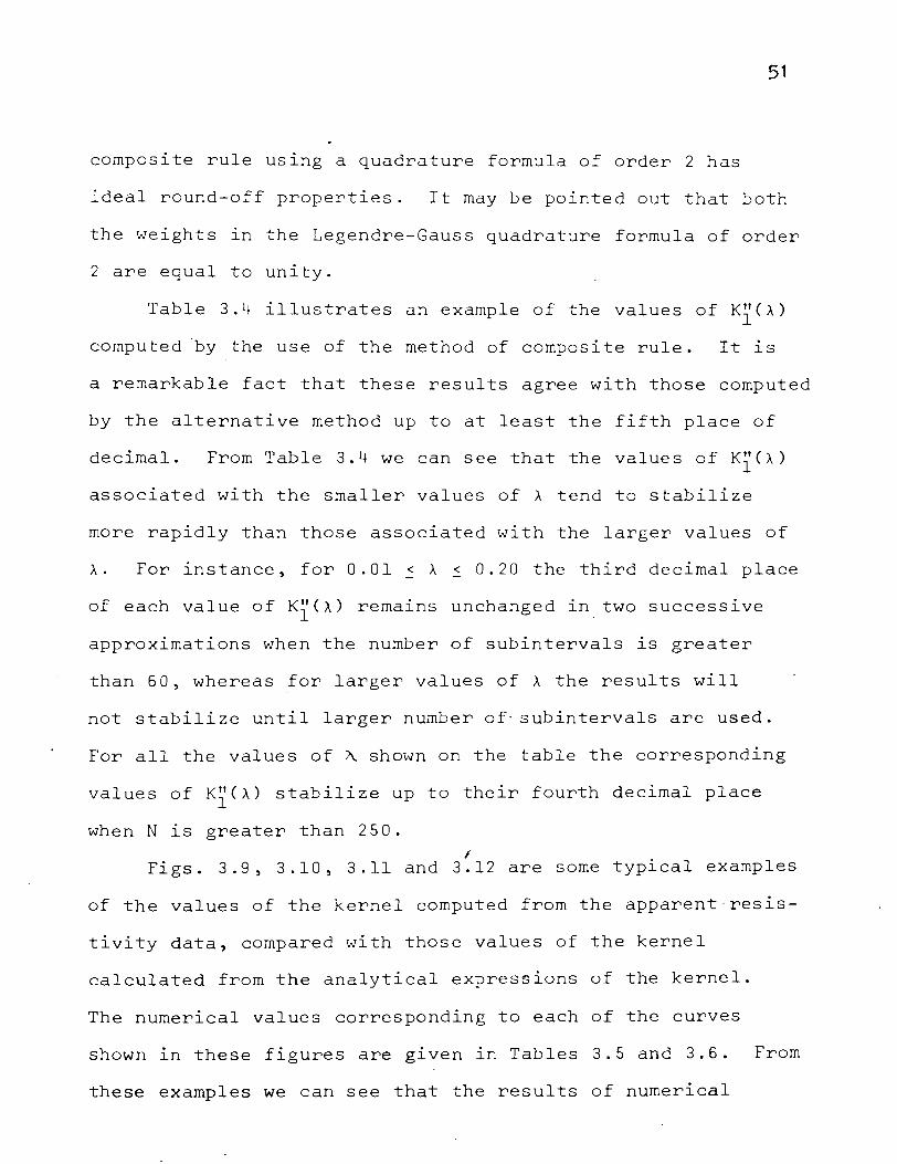
Figs. 3.9, 3.10, 3.11 and 3.12 are some typical examples

of the values of the kernel computed from the apparent·resis-

tivity data, compared with those values of the kernel

calculated from the analytical expressions of the kernel.

The numerical values corresponding to each of the curves

shown in these figures are given in Tables 3.5 and 3.6. From

these examples we can see that the results of numerical

1.0 r----r------~------------------------------

0.8

0.6

-~ tC 0.4 -~

0.2 -\_..1 o.o

-0.2

-0.4

0

\ \ \ \ \

\ \ \ \ . \ \ \ \ ' \

\ ,-1

\j I\ •

I I \ ' \ I '· \ I I\ \ "/ :X I \ 'r /, ~ I \ \ ,.'--'. '-· I - '"'

1 2 3

Fig. 3.8. Examples of the

{fA(t) -f")F(>.t) for

"' ... - '

4 5

"' > curves of the function

different values of "- •

52

TABLE 3.4

0.01

0.02

0.04

0.06

0.08

0.10

0.20

o.4d

0.60

0.80

1.00

1.20

1 .40

1. 60

t. 80

2.00

An example of the numerical values of K1' ( J\ ) obtained by the method of composite rule. n is the number of subintervals used.

53

Case f, -: f ... : fJ : f,. = 1 : 1 /3:3: 1/1 0, d 1 : d2 : d3 = 1 : 4 : 1

n=40 n=60 n=80 n=100

0.45128 0.45171 0.45185 0.45170

0.88866 0.88951 0.88979 0.88950

0.16758 0.16775 0.16780 o. 16775

0.23032 0.23058 0.23066 0.23058

0.27692 0.27726 0.27737 0.27725

0.31068 0.31110 0.31124 0.31110

0.38070 0.38153 0.38180 0.38152

0.42365 0.42516 0.42564 0.42514

0.46288 0.46418 0.46475 0.46414

0.48441 0.48631 0.48684 0.48623

0.49112 0.49253 0.49288 0.49237

0.48273 0.48307 0.48314 0.48278

0.46098 0.45952 0.45928 0.45908

0.42903 0.42490 0.42437 0.42428

0.39092 0.38319 0.38245 0.38238

0.35009 0.33787 0.33698 0.33686

54

TABLE 3.4 ( cont. ) -

n=150 n:200 n=250 n=300

0.01 0.45175 0.45174 0.45174 0.45173

0.02 0.88960 0.88957 0.88957 0.88956

o.o~ 0.16777 o. 16776 0.16776 0.16776

0.06 0.23061 0.23058 0.23060 0.23059

0.08 0.27729 0.27728 0.27728 0.27728

0.10 0.31115 0.31113 0.31113 0.31113

0.20 0.38161 0.38159 0.38159 0.38157

0.40 0.42531 0.42526 0.42526 0.42524

0.60 0.46436 0.46430 0.46431 0.46427

0.80 0.48645 0.48641 0.48641 0.48637

1.00 0.49246 0.49254 0.49254 0.49250

1. 20 0.48291 0.48290 . 0.48290 0.48287

1 .40 0.45911 0.45912 0.45912 0.45911

1.60 0.42422 0.42423 0.42423 0.42424

1.80 0.38224 0.38224 0.38224 0.38226

2.00 0.33665 0.33663 0.33663 0.33665

r 1 • 0

0.30

0.20

0.10

0 0 0 -o Curve obtained by numerical integration

~~--~x~x*-~~ Theoretical curve

55

0 ~--~--L---~--L---L---L---~--~--L---L---~~~--~~ 0

Fig.

2.0 2.5 3.0 0.5 1 .o 1 .5 ~----..,.

3.9. Kernel obtained by numerical integration and from theoretical formula. Case f, : f'L : /i : P. = 1 : 1 /3 : 3 : 1 11 o, d 1 : d 2 : d 3 = 1 : 4 : 1 •

1 .oo

r 0.90

o.so

0.70

0.60

0.50

0.40

0.30

0.20

o. 10

56

... ....o---o--- o- -o---o --o---o _ __,

~-o----o----o Curve obtained by numerical integration

,. " " a. - Theoretical curve

0 ~~~~--~--~--~--~---L--~--~--~--~--~--L-~ 0

Fig.

1 .o 2.0 2.5 3.0 0.5 1 • 5 ~----...

3.10. Kernel obtained by numerical integration and from theoretical formula. Case f. : ~ : {1 : f,. = 1 : 1 /3 : 3 : 1 1 1 o, d 1 : d 2 : d 3 = 1 : 3 : 2

1.00

0.90

o.so

0.60

o.so

0 .4Q!.

0.30

0.20

0.10

0 0 0.2 0.4

57

o-----._--~ Curve obtained by numerical integration

~ Theoretical curve

0.6 o.B 1 • 0 1 • 2 ~----~

Fig. 3.11. Kernel obtained by numerical inte~ration and from theoretical formula. Case f. : fa : r, : f-.. = 1 : 1 /3 : 3 : 1 I 1 o , d 1 : d 2 : d 3 = 1 : 2 : . 3 •

58

1.oor---~~--------------------------------------_,

0.60

o.so

0.40

0.30

0.20

0.10

0.2 0.4 0.6

Curve obtained by numerical integration

" Theoretical curve

0.8 1 • 0 "\. 1 • 2 "----~

Fig. 3.12. Kernel obtained by nureerical inte~ration and from theoretical formula. Case f, : f. : fS : f,. =

1 : 1/3 : 3 : 1/10, d1 : d2 : d3 = 1 : 1 : 4.

59

TABLE 3.5 Numerical values of the kernel obtained by integration of aprarent resistivity data and from theoretical forrr.ula. Case f, : ({ : ({ : f,.. = 1 : 1/3 3 1/10.

d1 :d2:d3= 1 4 d1 :d2:d3=1 3 . 2 . I II I II

0.01 0 ."151 o. 148 o. 177 0.175

0.02 0.199 0.1 95 0.249 0.247

0.04 0.284 0.280 0.372 0.372

o.o6 . 0. 352 0.349 0.463 0.465

0.08 0.405 0.401 0.524 0.526

o. 10 0.444 0.441 0.562 0.563

0.20 0.540 0.542 0.612 0.621

0.40 0.6~4 0.645 0.664 0.680

0.60 0.740 0.743 0.745 0.764

0.80 0.817 0.824 0.818 0.836

1 .oo 0.873 0.888 0.874 0.889

1 .20 0.913 0.934 0.913 0.928

1 .40 0.941 0.966 o. 941 0.955

1~60 0.960 0.984 0.960 0.975

1.80 0.973 0.994 0.973 0.989

2.00 0.982 0.998 0.982 0.998

2.20 0.988 0.999 0.987 1 .003

2.40 0.992 1 .coo 0.992 1 .oo6

2.60 0.995 1 .001 0.995 1 .007

2.80 0.996 1 .002 0.996 1 .007

I = theoretical values II = integrated values

60

TABLE 3.6 Numerical values of the kernel obtained by inte~ration of apparent resistivity data and from theoretical forr.JUla. Case f, : ({ : ~ : f,.. = 1 : 1/3 : 3 : 1/10

d1:d2:d3= 1 :2: 3 d1 :d2 :d3= 1 : 1 : 4

I II I II

. 0.01 0.204 o. 196 0.231 0.229

0.02 0.301 0.289 0.356 0.353

0.04 0.467 0.454 0.576 0.574

0.06 0.587 0.577 0.745 0.744

o.oa 0.665 0.659 0.862 0.862

0.10 0.709 0.707 0.934 0.937

0.20 0.728 0.732 0.969 0.974

0.40 0.712 0.721 0.851 0.867

0.60 o. 764 . 0.769 0.836 0.846

0.80 0.825 0.834 0.861 0.872

1 .oo 0.876 0.887 0.984 0.899

1.20 0.914 0.925 0.923 0.919

1 .40 0.941 0.952 0.945 0.937

1. 60 0.960 0.972 0.962 0.953

1.80 0.973 0.987 0.974 0.970

2.00 0.982 0.997 0.982 0.985

2.20 0.988 1 .003 0.988 0.997

2.40 0.992 1 .007 0.992 1 .005

2.60 0.995 1 .oo8 0.995 1 • 01 0

2.80 0.996 1 .007 0.996 1 • 011

I - theoretical values II = integrated values

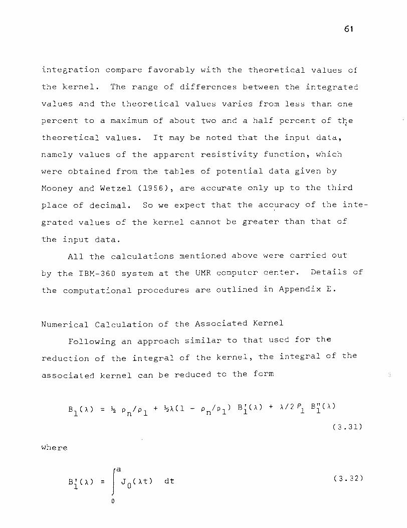
61

integration compare favorably with the theoretical values of

the kernel. The range of differences between the integrated

values and the theoretical values varies from less than one

percent to a maximum of about two and a half percent of the

theoretical values. It may be noted that the input data,

namely values of the apparent resistivity function, which

were obtained from the tables of potential data given by

Mooney and Wetzel (1956), are accurate only up to the third

place of decimal. So we expect that the accuracy of the inte-

grated values of the kernel cannot be greater than that of

the input data.

All the calculations mentioned above were carried out

by the IBM-360 system at the UMR computer center. Details of

the computational procedures are outlined in Appendix E.

Numerical Calculation of the Associated Kernel

Following an approach similar to that used for the

reduction of the integral of the kernel, the integral of the

associated kernel can be reduced to the form

where

Bi (A) = r J 0 ( ).t)

0

dt

(3.31)

(3.32)

and

Bl(A) = Jb(pa(t) - pn) J 0 (Atl dt

a

62

(3.33)

In the following we shall derive the formulas for the evalua-

tion of B{CA) and BlCA? respectively.

Integration of Bl(A). The calculation of Bl(A) lS quite

straightforward and can be achieved by the use of a single

Legendre-Gauss quadrature formula. By making the change of

variable,

t = a(y + 1)/2,

and then approximating the resulting integral with the

Legendre-Gauss formula (3.32) is transformed into

M L J 0 C~ aA(yJ. + ll)

j=l w.

J (3.34)

where y. and W. aga1n denote the abscissas and weights of the J J

quadrature formula.

Integration of Bl(A). As 1n the case of Kl(A), Bl(A)

can be calculated either by (i) the method of composite rule

or (ii) the method of approximating G(t) = pa(t) - Pn by a

parabolic arc. In this case the oscillating behavior of the

integrand is due to the Bessel function J 0 (At).

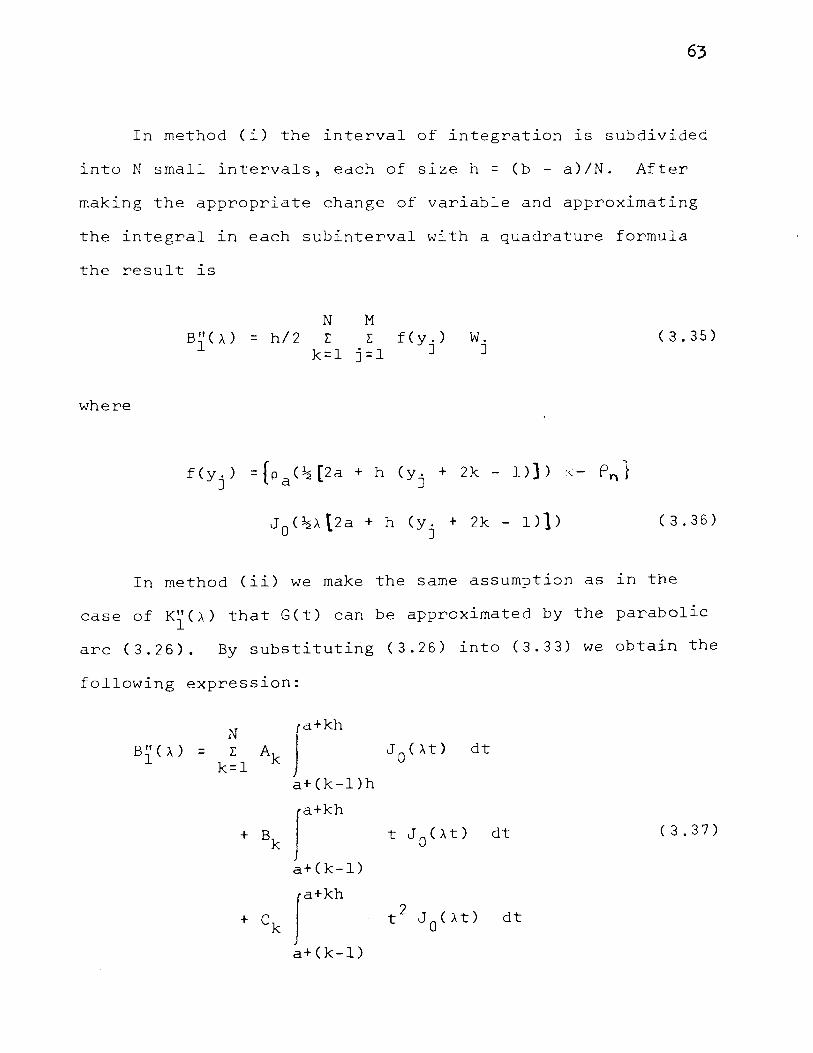
63

In method (i) the interval of integration is subdivided

into N small intervals, each of size h = (b - a)/N. After

making the appropriate change of variable and approximating

the integral in each subinterval with a quadrature formula

the result is

where

B"(>..) = l

N M h/2 E E

k=l j=l f( y.)

J w.

J (3.35)

(3.36)

In method (ii) we make the same assumption as ln the

case of Kl(>..) that G(t) can be approximated by the parabolic

arc (3.26). By substituting (3.26) into (3.33) we obtain the

following expression:

B"(>..) = l

+ Bk

+ ck

rkh a+(k-1) rkh a+(k-1)

dt

(3.37)

where the constants Ak, Bk, and Ck are glven by (3.27).

The second and third integrals of the above expression may

be integrated directly by noting that

and

+ x J (x) - I J 0 Cx) dx. 0 .

(Bowman, 1958). By carrylng out the integrations with the

aid of these two formulas (3.37) lS reduced to

dt

- (a+(k-l)h)(Bk+Ck(a+(k-1))) J1

CAta + (k-1)1)/A

64

( 3.38)

- (a+(k-l)h) J0

CA(a + (k-l)hl)}.

The integral which appears ln the first term of (3.38) can,

of course, be evaluated by means of a quadrature formula.

65

Some details of computation. From the equations derived

above one can see that the process for calculating the asso-

ciated kernel does not differ much from that for calculating

the kernel, with the exception that the function F(At) is now

replaced by the Bessel function J 0 CAt). So most of the

remarks made earlier concerning the calculation of K1 CA) can

equally be applied here. Consequently the following discus-

sions will be quite brief.

In the calculation of Bl(A) it was found that a single

quadrature formula of order between 10 and 20 was adequate

for all calculations in which 0 < A < 10 and 0.5 ~ a ~ 2.0.

Fig. 3~3 illustrates an example of the integrand

G(t)J0

CAt) associated with the integral of Bl(A). Like in

the case of G(t)F(At) the zeros of G(t)J 0 CAt) are more closely

spaced when the values of A are large than when the values of

A are small. Hence the number N of subintervals into which

the interval (a,b) of integration is going to be divided is

dependent on the value of A. Table 3.7 shows a set of values

of Bl(A) computed for a sequence of 40, 60, 80, 100, 150,

200, 250, 300 subintervals by the method of approximation by

a parabolic arc. One can see from this table that the

values of B"(A) stabilize to the fourth place of decimal when l

N is equal or greater than 250; these values associated with

small values of A tend to stabilize more quickly. Values

computed by the method of composite rule agree very closely

with these values shown here.

1 .oo

0.80

0.60

o.4o --tJ ~ -~ ~ 0.20 ~

..... ~

" 0 ~ ~

. ~0.20

-0.40

0

\ \ \ \

----'X..:'

\ \ \ \ \

~-,.., / \ I \ I,.... ·'"".. , ....

. I' \ / 'Y \ \;' \ \" 1\ \ ./ \ 1\ '\ \

I ' \ ,\ j \I \ . I ,, I

\ \ I • fJ \ ·~ J\ I ' , . ..,/· '..J/ ..,

1 2 3

t •

Fig. 3.13. Examples of the curves of the function

{,~(t) - ~) J0

( ~t) for different values

of ~.

66

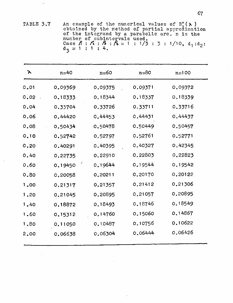
TABLE 3.7

0.01

0.02

0.04

0.06

0.08

o. 10

0.20

0.40

0.60.

0.80

1 .oo

1 • 20

1 .40

1. 60

1 .80

2.00

67

An example of the nurr.erical values of B" (-,... ) obtained by the method of partial approlimation of the integrand by a parabolic arc. n is the nu~ber of subintervals used. Case f,: ~: Ji :fit= 1: 1/3:3: 1/10, d 1 :d2 : d3 = 1 : 1 : 4.

n=40 n=60 n:80 n=100

0.09369 0.09375 0.09371 0.09372

o. 18333 o. 18344 0.18337 0.18339

0.33704 0.33726 0.33711 0.33716

0.44420 0.44453 0.44431 0.44437

0.50434 0.50478 0.50449 0.50457

0.52742 0.52797 0.52761 0.52771

0.40291 0.40395 0.40327 0.42345

0.22735 0.22910 0.22803 0.22823

0.19450 I o. 19644 0.19544 0. 19542

0.20058 0.20211 0.20170 0.20122

0.21317 0.21357 0.21412 0.21306

0.21045 0.20895 0.21057 0.20895

0.18872 o. 18493 0. 18746 o. 18549

o. 15312 0.14760 o. 15060 0.14867

0.11050 o. 10487 0. 10756 o. 10622

0.06638 0.06304 0.06444 0.06426

68

TABLE 3.7 ( cont. )

n=150 n=200 n=250 n=300

0.01 0.09372 0.09373 0.09373 0.09373

0.02 0.18340 0.18340. o. 18340 o. 18340

0.04 0.33717 0.33718 0.33718 0.33717

0.06 0.44440 0.44441 0.44441 0.44440

0.08 ·o.so46o 0.50462 0.50462 0.50461

0.10 0.52775 0.52777 0.52777' 0.52776

0.20 0.40353 0.40358 0.40357 0.40355

0.40 0.22839 0.22848 0.22844 0.22841

0.60 0.19567 0.19576 o. 19571 o. 19568

0.80 0.20157 0.20161 0.20157 0.20154

1.00 0.21350 0.21347 0.21344 0.21342

1 .20 0.20944 0.20932 0.20933 0.20931

1 .40 o. 18596 0.18576 o. 18580 0.18578

1 • 60 o. 14902 o. 14877 0.14883 0. 1 4881

1 .80 o. 10635 o. 10609 0. 10617 0.1 061 6

2.00 0.06405 0.06383 0.06391 0.06392

69

Typical examples of the curves of the associated kernel

obtained from the integration of the apparent resistivity

data are shown in Figs. 3.14, 3.15, 3.16, and 3.17. On these

figures are shown also the corresponding theoretical curves

of the associated kernel. The numerical values for these

curves are given in Talbs 3.8 and 3.9. These examples show

that there is a general close agreement between the theoreti

cal and the integrated values of the associated kernel.

Again, it may be noted that the input resistivity data were

obtained from the tables of potential data given by Mooney

and Wetzel.

The computational procedures are outlined 1n Appendix E.

Some Possible Sources of Error

Apart from the errors that are inherent in the integra

tion formulas there are several other factors which may

influence the results of integration of both the kernel and

the associated kernel. Since the apparent resistivity func-

tion is only known empirically the accuracy of the input

values of the apparent resistivity function 1s obviously one

of the influencing factors. Because of the fact that a

un1que correspondence exists between the apparent resistivity

function and the kernel Cor the associated kernel) one may

expect that the result of the numerical integration will be

sensitive to any variations in the input apparent resistivity

data. The closeness of fit between the least-squares

70

polynomial and apparent resistivity data would be another

influencing factor. Generally speaking the greater the num-

ber of data points the better the least-squares approximation

will be. In all our calculations sixteen data points were

used and the results were satisfactory.

In the derivation of the integration formulas we made

the assumption that the resistivity of the top and bottom

layers could be determined if measurements were made with

very short or very long electrode separation. In practice

some uncertainty may exist in the determination of the values

of a and b, and also that of pl and Pn· Thus this is another

factor that may influence the result of integration. Under

normal field conditions a can be determined with a high

degree of precision while b can only be determined approxl-

mately. This is indeed quite fortunate in the sense that

error in the measurement of a will have a greater influence

on the result of integration than that in the measurement of

b because the terms in the quadrature formulas near the upper

limit of the integral generally have negligible contribution

to the total sum owing to the fact that both the functions

G(t) and J 0 CAt) Cor f(At)) are very small in magnitude near

the upper limit of the integral. With regard to the resis-

tivity of the top and bottom layers, information on them is

often available from other external sources. If this infor

mation is available it will be of great help in our computa-

tion.

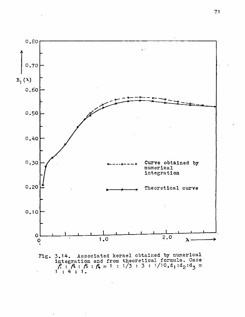
71

o.sor---------------------------------------------~

) 0.70

0.30

0.20

o. 10

-·

--

o----o---o Curve obtained by numerical integration

• Theoretical curve

0~~--~---L--~--i---L-~--~--~--~--L-~--~~~ 0 1.0

Fig. 3.14. Associated kernel obtained by numerical integration and from theoretical formula. Case f, : f.. : 11 : f .. = 1 : 1 /3 : 3 : , I 1 o, d 1 : d2 : d3 = 1:4:1.

0.80

0.60

0.50

0.40

0.30

0.20

0.10

0

72

---4---.--..J

0

o---o--.... Curve obtained by numerical integration

••--~•~--1- -Theoretical curve

Fig. 3.15. Associated kernel obtained by numerical integration and from theoretical formula. Case f, : fa : t~ : r,. = 1 : 1 /3 : 3 : 1 I 1 o , d 1 : d 2 : d 3

- 1 : 3 : 2.

0.80

f 0.70

0.50

0.40

0.20

/.

~ /

-o--..._ ,~ -·--

/ -

o---o---o Curve obtained by numerical integration

• Theoretical curve

Fig. 3.16. Associated kernel obtained by numerical integration and from theoretical formula. Case

f, : /{ : ft : f.- = 1 : 1/3 : 3 : 1/1 0, d 1 : d2: d3 = 1 : 2 : 3.

73

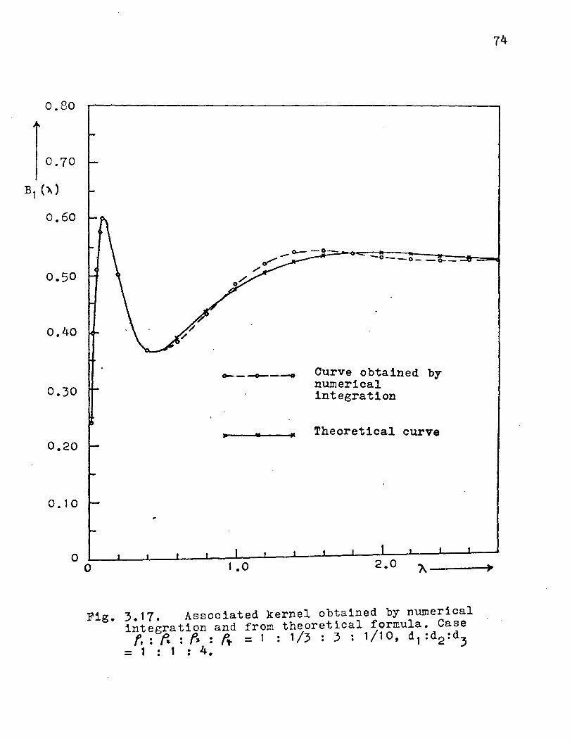
0.80

0.70

Bl (l.)

0.60

o.so

0.40

0.30

0.20

0.10

0 0

-o--o- -o--

~--o---o Curve obtained by numerical integration

~---~·~--~~ Theoretical curve

1.0 2.0

Fig. 3.17. Associated kernel obtained by numerical integration and from theoretical forreula. Case

f, : ~ : f, : t;. = 1 : 1 /3 : 3 : 1 /1 0' d 1 : d2: d3 = 1 : 1 : 4.

74

75

TABLE 3.8 Numerical values of the associuted kernel obtained by inteeration of apparent resistivity data and from theoretical formula. Case f.: ~ : ~ : f,. = 1 : 1/3 : 3 : 1/10

d1 :d2:d3= 1 . 4. . . 1 d1 :d2:d3= 1 . 3. . . 2

I II I II

0.01 0.088 0.086 o. 108 0. 106

0.02 0.123 0.121 0. 1 61 0.159

0.04 o. 184 o. 183 0.248 0.248

o.o6 0.231 0.230 0.306 0.308

0.08 0.263 0.262 0.338 0.339

o. 10 0.284 0.284 0.351 0.351

0.20 0.318 0.323 0.331 0.337

0.40 0.374. 0.377 0.358 0.368

0.60 0.444 0.449 0.430 0.439

0.80 0.495 0.503 0.486 0.493

1.00 0.526 0.538 0.521 0.530

1.20 0.543 0.557 0.541 0.551

.1 .40 0.550 0.566 0.549 0.561

1 .60 0.552 0.567 0.551 0.562

1 .80 0.549 0.563 0.549 0.558

2.00 0.545 0.556 0.545 0.552

2.20 0.540 0.547 0.540 0.544

2.40 0.535 0 • .539 0.535 0.537

2 •. 60 0.530 0.531 0.530 0.530

2.80 0~526 0.524 0.526 0.525

I - theoretical values II = integrated values

TABJ-'E 3.9

0.01

0.02

0.04

0.06

o.o8 o. 10

0.20

0.40

0.60

0.80

1.00

1.20

1. 40

1.60

1 .80

2.00

2.20

2.40

2.60

2.80

76 Numerical values of the associated kernel obtained by integration of apparent resistivity data and from theoretical formula. Case f. : {{ : /{ : f~ = 1 : 1 /3 : 3. : 1 I 1 o

d1 :d2:d3= 1 :2: 3

I II

o. 128

0._199

0.317

0.393

0.431

0.442

0.373

0.348

0.411

0.469

0.509

0.532

0.544

0.548

0.548

0.544

9.540

0.535

0.530

0.526

0.122

0.191

0.308

0.388

0.431

0.445

0.374

0.348

0.405

0.469

0.522

0.554

0.568

0.568

0.560

0.549

0.539

0.531

0.525

0.522

d 1 : d2 : d3 = 1 : 1 : 4

I II

o. 148

0.241

0.397

0.509

0.574

0.601

0.502

0.367

0.389

0.436

0.476

0.504

0.522

0.531

0.535

0.535

0.534

0.531

.0.527

0.524

o. 146

0.238

0.396

0.508

0.574

0.600

0.499

0.368

0.380

0.436

0.483

0.521

0.538

0.540

0.535

0.528

0.523

0.522

0.523

0.527

I = theoretical values II - integrated values

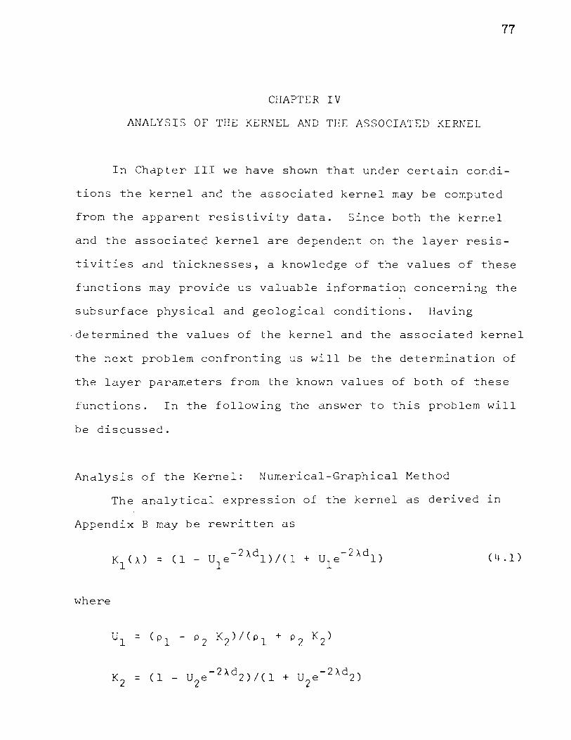
77

CHAPTER IV

ANALYSIS OF THE KERNEL AND THE ASSOCIATED KERNEL

In Chapter III we have shown that under certain condi-

tions the kernel and the associated kernel may be computed

from the apparent resistivity data. Since both the kernel

and the associated kernel are dependent on the layer resis-

tivities and thicknesses, a knowledge of the values of these

functions may provide us valuable information concerning the

subsurface physical and geological conditions. Having

,determined the values of the kernel and the associated kernel

the next problem confronting us will be the determination of

the layer parameters from the known values of both of these

functions. In the following the answer to this problem will

be discussed.

Analysis of the Kernel: Numerical-Graphical Method

The analytical expression of the kernel as derived 1n

Appendix B may be rewritten as

( 4 .1)

where

. . . . . . . . . . . . . . . . . . . . . . . . . . . . . . . . . . . . . . . . . . . . . . . . . . . . . . . . . . . .

K. = (1 - U.e- 2 Adi)/(l + U.e- 2 Adi) l l l

. . . . . . . . . . . . . . . . . . . . . . . . . . . . ...

. . . . . . . . . . . . . . . . . . . . . . . . . . . . . ..

K = (l - U 1e- 2 Adn-l)/(l + U e- 2 Adn-l)

n-1 n- n-1

u n-1 = k n-l,n = (p 1- p )/(p 1 + p ). n- n n- n

To analyze this function we begin with the simplest case,

namely the two-layer case, and then proceed to the three-

layer case, after which the analysis will be generalized to

the n-layer problem. The general procedure of the analysis

78

presented here is quite similar to that of Pekeris (1940) in

the sense that our method is also a numerical-graphical method

which depends on the behavior of the kernel at largeA. How-

ever, the details of our analysis are totally different from

those of Pekeris's method and also the kernel defined here

is not identical with that employed by Pekeris in his analysis.

Two-layer case. In (4.1) if we put n = 2, we obtain the

kernel for the two-layer case:

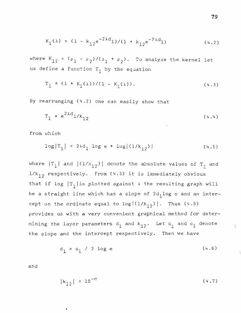
79

( 4 . 2 )

where K1 2 = (pl- P 2 )/(pl + P 2 ). To analyze the kernel let

us define a function T1 by the equation

( 4. 3)

By rearranging (4.2) one can easily show that

( 4. 4)

from which

( 4 • 5 )

where IT 1 j and jCl/k12 )1 denote the absolute values of T1

and

l/k12 respectively. From (4.5) it is immediately obvious

that if log jT1

jis plotted against A the resulting graph will

be a straight line which has a slope of 2d1 log e and an inter

cept on the ordinate equal to logj(l/k12 ) I. Thus (4.5)

provides us with a very convenient graphical method for deter-

mining the layer parameters d1 and k 12 . Let s1

and c 1 denote

the slope and the intercept respectively. Then we have

d1

= s 1 I 2 loge (4.6)

and

l k I = 10-c 12

( 4 • 7)

80

It may be noted that the reflection factor k 12 may take on

any value lying in the interval (-1,1). The result given by

(4.7) does not indicate whether k 12 is positive or negative.

But it will be shown later that the sign of the reflection

factor is related to the sign of the function T1 . Assuming

that the sign of the reflection factor is known then f 2 can

be calculated from

C4.S)

slnce P1

lS already known from direct field observations.

Three-layer case. By putting n = 3 one gets the three-

layer kernel:

(4.9a)

where

(4.9b)

(4.9c)

(4.9d)

The procedure for analyzing this three-layer kernel may be

outlined as follows:

(i) Determination of d1

and k 12 --Again uslng (4.3) as the

81

definition of T1 one can show from (4.9a) that

(4.10)

from which one gets

(4.11)

We note that in this case log IT1 1 is no longer a linear

function of A because the function Ul lS also dependent on A,

but it will approach a linear function when ~ becomes large.

f . h f . -2Ad At large values o A, s1nce t e unct1on e 2 whose magn1-

tude decreases rather rapidly with the increase of A becomes

negligible we may make the following approximations:

k -2Ad 2 O 23e ~ It follows that when

becomes large the function log IT1 1 should approach asympto

tically to the straight line

where s1

= 2d1

loge and c 1 = log ICl/k12 ) I. Hence d 1 and k 12

can be determined from the slope and the intercept of the

asymptotic straight line respectively.

(ii) Determination of d 2 and k 23 -- Since d 1 lS known from

the result of step (i) u1 can be computed from (4.10), that

lS,

(4.12)

82

From (4.9b) we obtain

(4.13)

from which K2 can be calculated.

leads to the equation

The rearrangement of (4.9c)

(4.14)

It follows that

(4.15)

Equation (4.15) represents a straight line with slope

s 2 = 2d 2 log e and intercept c 2 = log!Cl/k 23 )!. Thus the

layer parameters of the three-layer problem are completely

determined.

Generalization to n-layer case. The kernel for the

n-layer case is given by (4.1). To determine the layer para

meters from this kernel we merely extend the procedure employed

for the decomposition of the three-layer kernel as follows:

(i) Determination of d1

and k 12 --In this case d1 and k 12

can be determined in exactly the same manner as in the three-

layer problem. Using similar arguments as before we can show

that the function

(4.16)

83

should approach asymtotically to the straight line

where s 1 = 2d1 loge and c 1 =log (l/k12

). Thus d1

and k12

are determined.

Cii) Determination of d 2 and k 23 -- By letting T2

to denote

(l + K2 )/(l - K2 ) one can show that

(4.17)

Since U2 approaches k 23 at large ), (4.17) will approach the

straight line

where s 2 = 2d 2 loge and c 2 = log !Cl/k23 ) I.

d 2 and k 23 can be determined.

From s 2 and c 2

(iii) Determination of k .. +l and d. --By repeating the l 'l l

process described ln step Cii) the layer parameters for each

successive deeper layer can be obtained. Assuming that the

parameters of the first i-1 layers have been determined we

wish to solve for k .. +l and d. now. To do this we make l,l l

use of the following equations:

= 2>,d._l/T U. 1

e l . 1 l- l-

(4.18)

K. = p. l (l- U. 1 )/p.(l + U. l) l l- l- l l-(4.19)

84

log jT.j = 2:\d. loge+ log jCliU.)j l l l (4.20)

where T. = ( 1 + K.) I ( 1 - K.). Since U. approaches K. . 1 l l l l l,l+

at large :\ the function log IT.I will approach its asymptote l

Y. = :\s. +c. l l l (4.21)

where s. = l 2di loge and ci =log (11ki,i+l). It follows

that

and

d. = s. I 2 log e, l l

lk .. +11 l,l = 10-c

'

where 1 = 2, 3, 4, ..... ,n-2.

(4.22a)

(4.22b)

(4.22c)

Civ) Determination of k 1 and d 1 -- U 2 and K 1 can n- ,n n- n- n-

be obtained from (4.18) and (4.19) respectively by putting

i = n-1. Since U 1

= k = ( p 1

- p ) I ( p 1

+ p ) , it n- n-l,n n- n n- n

is clear from (4.20) that

log jT l = 2:\d 1 loge+log jCllk 1 )j n-1 n- n- ,n

Equation (4.23)represents a straight line with slope

sn-l = 2dn-l loge and intercept cn-l =log Cllkn-l,n).

follows that

(4.23)

It

d n-1 (4.24a)

85

lk I = 10-c n-l,n (4.24b)

= Pn-1 (1-k 1 )/(1 + k 1 ). n- ,n n- ,n (4.24c)

Discussion of examples. In order to illustrate the pro-

cedure of analysis discussed above we shall consider some

examples. Again we shall begin our discussion with the two-

layer case.

The two-layer case compr1ses a top layer of resistivity

pl and thickness d 1 , and a substratum of resistivity p 2 and

infinite thickness. Examples of the kernels associated with

two-layer structures are g1ven in Figs. 4.1 and 4.2. In

Fig. 4.1 are shown the kernels associated with these cases 1n

which the reflection factors are positive while those ker-

nels shown in Fig. 4.2 are associated with two-layer struc-

tures with negative reflection factors. It may be noted

that all these curves of the kernel were computed from the

analytical expression (4.2).

The first step in the analysis of a two-layer kernel

involves the calculation of T1 from (4.3). The general rela-

tionship between T1 and K1 (A) as defined by (4.3) is illus-

trated in Fig. 4.3. There are two things to be noted from

Fig. 4 . 3 . First, the function Tl possesses an infinite

discontinuity when K1

(A) takes on the value of unity. The

next thing to be noted lS that Tl > 0 if K1 (A) < 1 and Tl < 0

if Kl(>.) < 1. Thus from Figs. 4.1 and 4. 2 it lS evident that

1.00 r-------------------------------------------

0.90

0.70

0.60

o.so

0.40

0.30

0.20

o. 10

0.2 0.4 0.6 0.8 t.o 'h 1.2

Fig. ~.1. Curves of two-layer kernels with positive reflection factors

86

10.0~----------------------------------------------~

9.0 Kl ()>.)

8.0

7.0

6.0

5.0

4.0

3.0

2.0

1. 0 ---- ---- -~- --- - -

Fig. 4.2. Curves of two-layer kernels with negative reflection factors.

87

88.

1 o.o r-------r---.-----------~

0

-2.0

-4.0

-6.0

-8.0

I -------------------

1 I I I I I I I I I I

·10.0L-~--L-~--~~--~~~~--~~--~~~ 0 1.0 2.0

Kl (")

Fig. 4.3. Relation between K1 (~)and T1 •

the positive values of T1 will be associated with positive

reflection factors because in such cases K1

(A) < 1, while

the negative values of T1 will be associated with negative

reflection factors because K1 (A) > 1 for such cases. Further-

more one may note that in any two cases in which the reflec

tion factors are of the same magnitude but of opposite signs

the T1 's will have the same absolute values, providing that

d 1 is the same for both cases. Thus the graphs of log IT1

1

plotted against A are identical in all cases which have the

same absolute value for k 12 and the same thickness d1

.

Examples of the graphs of log IT 1 1 plotted against A corres

ponding to the kernels shown in Figs. 4.1 and 4.2 are

illustrated in Fig. 4.4. The fact that all the graphs are

straight lines is clear from (4.5).

From each of the graphs shown in Fig. 4.4 one can deter-

mine the absolute value of k 12 and d 1 . One can easily

estimate that the slope s 1 is equal to 0.8686. By substitut

ing this value of s 1 into (4.6) one gets d 1 = 1.0. To

determine the absolute value of k 12 one merely extends each

graph to intercept the vertical axls. The value of each

intercept on the vertical axis is shown in Fig. 4.4. The

absolute value of k 12 is given by the reciprocal of the value

of the intercept shown in the figure. The correct sign of

each reflection factor has to be determined from the sign of

T1 associated with each case as it has been pointed out in

the previous paragraph.

In practice it may not be necessary to carry out the

calculation of the slope s1

. d1

can easily be determined

graphically. Let us consider the equation

log Y = Ad log e y > 0

90

If d is considered to be a parameter, then by ass1gn1ng dif

ferent values of d to the above equation we can construct a

master diagram which consists of a series of straight lines,

each line corresponding to one of the values of d. fig. 4.5

is an example of such master diagram. With the aid of a

master diagram of some suitable scale one can determine d1

as follows: Plot the graph of log IT 1 1 vs. A on a tracing

paper using a scale identical with that of the master diagram.

Then superimpose the tracing on the master diagram with the

vertical axes coinciding with each other. The tracing is

moved until the plot on it fits one of the straight lines on

the master diagram. Then the value of d 1 will be given by

one-half the value of d associated the line that fits the

graph on the tracing.

Next, let us consider the analysis of the three-layer

kernels. The three-layer case compr1ses a top layer of thick.-

ness d1

, a middle layer of thickness d 2 , and a bottom layer

that is theoretically assumed to extend to infinity. There

are an infinite number of permutations and combinations

of resistivity contrasts of the three beds. However, there

are only three main groups of possibilities concern1ng the

resistivity of the middle layer in relation to that of the

91

others: it may be higher than, lower than, or intermediate

between the resistivities of the top and bottom layers.

Accordingly the resistivity curves are conveniently divided

into four categories; (i) pl > p2 < p 3 ' (ii) pl < p2 > p 3'

(iii) pl < p2 < p 3 ' and (iv) pl > p2 > p 3. Generally the

sounding curves belonging to each category have a character-

is tic shape (see Fig. 4 . 6 ) . This property of the sounding

curves has often been utilized qualitatively for interpreta

tive purposes. The curves of the kernels corresponding to

these four categories of three-layer situations also exhibit

similar characteristics. Figs. 4.7, 4.8, 4.9, and 4.10 are

typical examples of the three-layer kernels.

Since the procedure for analyzing the three-layer kernels

ls identical for all cases, it is sufficient for us to

consider the case shown in Fig. 4.7. The values of the laye~

resistivities and thicknesses assumed for the computation of

these curves are pl = 1, p 2 = 10, p 3 = l/10, d1 = l, and

d 2 = 4, 1~, 2/3, and\ respectively. The reflection factors

corresponding to the given values of the resistivities are

k12 = -0.82 and k 23 = 0.98. These kernels are analyzed

according to the procedure discussed in the previous section;

the results of the analyses are shown in Figs. 4.11, 4.12,

4.13, and 4.14.

Refering to the results of analyses shown in Figs. 4.11,

4.12, 4.13, and 4.14 one can see that for small values of the

function log jT1

) is not linearly related to A but it approaches

92

the linear relation

rather rapidly at large values of A. This behavior of

log !T 1 1 lS ln accordance with that predicted by (4.11). The

parameters d 1 and jk12 1 can easily be determined from the

asymptotic portion of the curve of log jT1

j with the aid of a

master diagram similar to the one shown in Fig. 415, but

plotted with some suitable scales. It is of interest to note

that in practice the non-linear relationship between log jT1

j

and A at small values of A could serve as a useful guide to

the fact that the problem under consideration is one involv-

1ng more than two layers. So when this type of relationship

is observed further decomposition is necessary in order to

determine the parameters of the lower layer Cor layers).

In the second stage of decomposition (4.12) and (4.13)

are used to compute the function T2 . The resulting graphs of

log IT 2 1 plotted against A for all the four cases are straight

lines, thus indicating that no further discontinuity exists

beneath the second layer. The layer parameters d 2 and k 23

can again be determined with the aid of a master diagram of

some suitable scales.

As in the two-layer case the study of the behavior of

the function T1

may throw some light on the nature of the

reflection factor k 12 . Fig. 4.15 illustrates curve 4 of

Fig. 4.7 together with the curve of the associated T1 .

93

The curve of T1 shows the presence of a discontinuity 1n the

neighbourhood of the point A = 3.6 at which the curve of K1

(A)

intersects the line K1

(A) = 1. One may also note that the

sign of T1 changes from positive to negative as one crosses

the discontinuity from the left to the right. This change in

sign of T1 is related to the fact that K1

(A) < 1 when A < 3.6

and K1

(A) > 1 when A > 3.6. It is clear that the T1

's

associated with the kernels of the remaining three cases

shown in Fig. 4.7 will behave in a similar manner. On the

other hand one may expect that the T1

's associated with the

kernels of the case p 1 : p 2 : p 3 = 1: 1/10: 10 shown in Fig. 4.8

will behave in an opposite manner, that is, the sign of T1

changes from negative to positive as the discontinuity is

crossed from the left to the right. The reason lS simply that

K1 (;.) > 1 to the left of the discontinuity and K1

(;.) < 1 to

its right. Fig. 4 .16' for instance, shows the

associated with the case d1

= 0.25 of Fig. 4.8.

cases p = 1: 3

3: 10 and p 1 :

function Tl

For the

(Fig. 4.9 and Fig. 4.10 respectively) the function T1 does

not possess any discontinuity because K1 (;.) is either greater

or smaller than unity throughout the entire range of !..

From the above observations we note that in the first

cases, namely p • p • p = 1: 10: 1° 2. 3

1/10: 10, T1

is positive beyond the point of discontinuity if

the reflection factor k 12 is positive and lS negative if k 12

1s negative. In the remaining two cases, similar relationships

94

exist between T1 and k 12 . Thus by noting the slgn of the

values of T1 one can determine the correct sign of k 12 .

Actually the above conclusion can be predicted from

(4.9), the analytical expression for the kernel. It has

already been pointed out that when \ is large u1 approaches

k 12 and thus the kernel of a three-layer case lS reduced

essentially to that of a two-layer case. In the analysis of-

the two-layer kernels we observe that positive values of T1

are related to positive reflection factors and negative values

of T1

are related to the negative reflection factors. Thus

we expect that the T1

's of the three-layer cases will behave

ln a similar manner at large values of A .

Refering to (4.9c) we can see that the expresslon for

K2

is actually the kernel function for a two-layer structure

with a reflection factor equal to k 23 , the thickness of its

top layer being equal to d2

. It is, therefore, clear that T2

will be related to k23

in exactly the same way as T1 is

related to k12

. In other words, T2 is positive if k 23 is

positive and T 2 is negative if k 23 is negative.

Since the analysis of the kernels of other multilayer

problems is identical to that of the kernels of the three

layer case, we shall not consider any further examples. An

example of the analysis of the four-layer kernels is given in

Appendix F.

I T11

loo.or--------------------------------------------80.0

60.0

50.0

40.0

30.0

20.0

10.0

8.0

6.0

5.0

4.0

3.0

2.0

1 .o 0

Fig.

o· ").. \ ~

\"~-' ...

0.2 0.4 0.6 0.8 1 .o ~ )l

4.4. Log IT 11 vs. " • Analysis of two-layer kernels.

95.

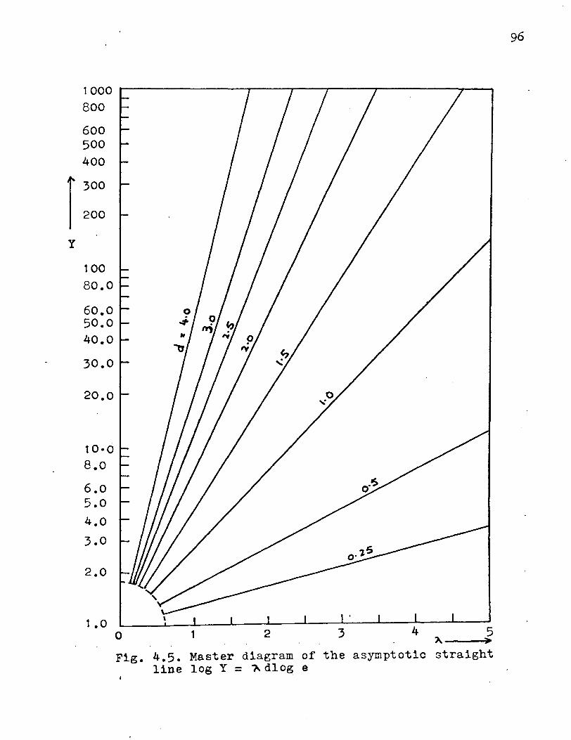
r y

1000 800

600 500 400

300

200

100 80.0

60.0 50.0 40.0

30.0

20.0

10·0 8.0

6.0 5.0

4.0

3.0

2.0

1 .o 0 1 2 3 4 5

~ > Fig. 4.5. Master diagram of the asymptotic straight

line log Y = ~ dlog e

96

fa.Ct)

f. > f ... < ~

t

I I I I I I I I I

fa-Ct>

1-r-----1 t

97

--------,---------fa (t)

f. < f .. < fi

t

1

I I I I I I I I I I I

fl,.c t >

t

Fig. 4.6. Classification of three-layer apparent resistivity curves according to their characteristic shapes.

3.2

r 2 ·8

Kl ("')

2.4

2.0

1 .6

1 • 2

0.8

0.4

d1 : d2= G) 1 . 4 . @ 1 . '1 .A. . 2

G) 1 . 2/3 . ® 1 1/4

K.c ... ) : a-o

Fig. 4.7. Curves of three-layer kernels for the case f. : f'L: f~ = 1 : 10 :· 1/10

98

99

4.or--------------------------------------------

3.6

3.2 d1 d2 = CD 1 . 4 . ® 1 • 1i . G) 1 • 2/3

2.8 .

® 1 • 1/4 . K1 (~)

2.4

2.0

1 .6

1. 2

----------

0.8

0.4

0~----~------~------~----~~----~------~----~ 0 0.2 0.4 0.6 0.8 1 • 0 1 • 2

"----~ Fig. 4.8. Curves of three-layer kernels for the case

f. : {{ : f, = 1 : 1/1 0 : 1 0.

100 1.o.---------~~----------------------------------

0.9

l 0.8

d1 d2 = 0) 1 . 4 . ® 1 . 1-l .

K1 ( ~) G) 1 . 2/3 . ® 1 • 1/4

0.7 .

0.6

o.B

0.4

o.3

·- ::--- ----0.2

o. 1

0~----~------~----~------~------L------L----~ o o.2 o.4 o.6 o.B 1.0 1.2 1.4 A---~

Fig. 4.9~. Curves of three-layer kernels for the case f. :f.. =f~ = 1 : 3 : 10.

/

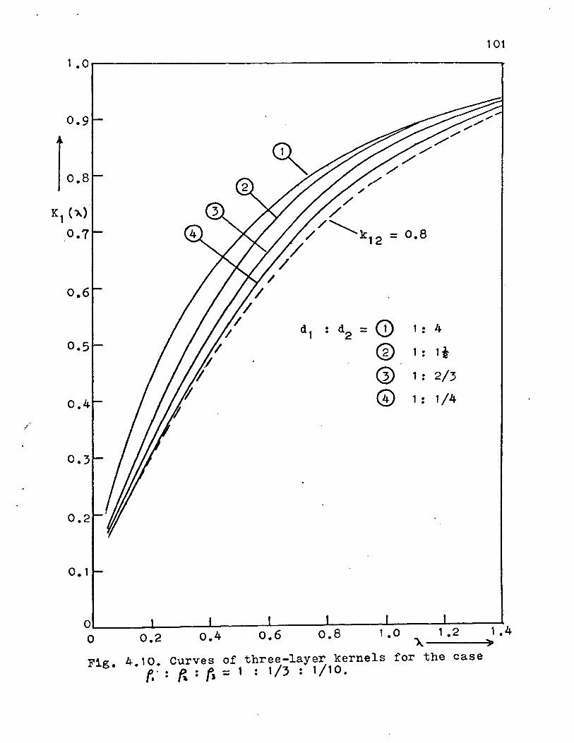
101 1-0r---------------------------------------------

0.9 ,.. ,.,.

I o.e

// /

/ /

/ /

/ K1 ( ") /

0.7 /~ = 0.8 / k12

/ /

0.6

d1 . d2 G) 1 • 4 • - .

0.5 @ 1 : li

G) 1 : 2/3

0.4 ® 1 : 1/4

0.3

o. 1

0------~------~----~------~----~------~----~ 1.0 1.2 1.4 0 0.2 0.4 o.6 o.B

~----~')'

Fig. 4.10. Curves of three-layer kernels for the case f. · : f{ : r, = 1 : 1 /3 : 1 I 1 o .

100r-------------------------~------------------

50

4o

30

20

10

8

6

5

4

3

2

2 Xd 1log e +

I( 1 /k12 >I

1 0 0.2 0.4 0.6 0.8 1 .o

ker-nel ). ~ Fig. 4.11. Analysis of three-layer~of the case

f. : ~ : f, = 1 : 10 : 1/10, d1 : d2 = 1 : 4.

102

103

100r---------------------------------~------~

10

8

6 5

4

3

2

logiT 1J vs. "'

___ Asymptote Y1

= 2 '). d1log e +

~ 1 /k12 >I

= 1.22

- 1 .01

Fig. 4.12 Analysis of three-layer kernel of the case f. : fa. : f, = 1 : 1 o : 1 I 1 o, d 1 : d 2 = 1 : 1 i.

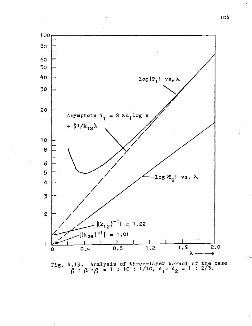
104

100r-------------------------------------------

so

60 50

4o

30

20

10

8

6

5

4

3

2

1 0

Asymptote Y1

+ J( 1 /k12 )I

0.4 0.8

= 1.22

1 • 2 1.6 2.0 }..--~)

Fig. 4.13. Analysis of three-layer kernel of t~e case f, : f.. ={{ = 1 : 10 : 1/10, dl: d2 = 1 : 2/3.

105

500 r-----------------------7---------------~ 400

300

200

100

80

60

50 40

30

20

1rG

8

6 5 4

3

Y 1 = 2 ~ d 1 1 og e +

I< 1 /k12 >I

VS • "

2.0 3.0 4~0 5.0 ~-~>

Fig. 4.14. Analysis of three-layer kernel of the case f, : fa: {i = 1 : 10 : 1/10, d1 : d2 = 1 : 1/4.

i T1

,.

106

50 I 2.0 i I

T1--

-10

-20

-30

-40

I I I I I I I

I K1 ( ") /

k· (Jt. \ 2 1·0 -- _.____. __ ---I I

I I I I I I I I I r

...

1 • 8

1 • 6

1 .4

-50L--L--~~~~~~--~~--~~~~--~~o 0 0.2 0.4 0.6 0.8 1 .o 1 .2

~---~

Fig. 4.15. The function T1 and its related threelayer kernel. Case f. :f. : 8 = 1 : 10 : 1/10, d 1 : d 2 = 1 : 1 14 .

K1 ( ~)

l T1

50

T~ 1

I I I I I I I I I I I

_K-t-1"'1..=_1 _____ _

107

.o 1 K 1 (>t)

.6

.2

.8

.4

-40

-so~~~~--~~~~--~--~~--~--~~~~o 0 0.2 0.4 0.6 0.8 1 .o 1 .2

A---~

Fig. 4.16. The function T1 and its related threelayer kernel. Case f. : f&.: {1 = 1 : 1/10 : 10, d 1 : d 2 = 1 : 1 14 .

108

Analysis of the Associated Kernel: Numerical-Graphical Method

The associated kernel has been shown to be related to

the kernel by the equation

K1

(A) lS expressed explicitly by (4.1) while K1 (A/2) may be

obtained from (4.1) by replacing A with A/2. Thus after sub-

stituting A = A/2 into (4.1) we get

where

. . . . . . . . . . . . . . . . . . . . . . . . . . . . . . . . .

. . . . . . . . . . . . . . . . . . . . . . . . . . . . . . . . .

. . . . . . . . . . . . . . . . . . . . . . . . . . . . . . ...

. . . . . . . . . . . . . . . . . . . . . . . . . . . . . . . ..

K' n-1 = k e-Adn-1)/(1 + k e-Adn-1)

(l - n-l,n n-l,n

k = (p - p )/(p 1 + p ). n-l,n n-1 n n- n

(4.25)

109

Although the associated kernel appears to be a more

complicated function than the kernel similar technique of

decomposition can be used to determine the layer resistivi-

ties and thicknesses.

Two-layer case. From (4.1) and (4.25) the associated

kernel for the two-layer case is found to be given by the

equation

1 Bl(A) =

1 +

from which it can

2 B1

(A) + 1

2B1

CA) - 1

When A is large,

k -2Adl 1 12e k -2Adl

~

12e 1

be shown that

Slnce k 2 -3>..dl 12e

the following approximation:

2B1

(>..) + 1

2B1

CA)- 1

By letting

we have

-Ad k 12 e 1

-Ad (4. 26) + k 12 e 1

-Ad e 1 + 2 kl2

(4.27)

11 0

for large values of A. It follows that

(4.28)

which is the equation of a straight line with slope s1

= (d1

log e)and intercept c 1 = logj(l/k12 )j. Thus d1 and k12

are

derivable from c 1 and s 1 which are associated with the

asymptote of the function logjQ 1 1.

Three-layer case. The associated kernel for the three-

layer case is given by

( 4 • 2 9 )

where ul is glven by (4.9a) and

(4.30a)

(4.30b)

To analyze the associated kernel we may proceed as

follows:

(i) Determination k12

and d1 --From (2.29) it can be shown

that

28l(A) + 1

28l(A) - 1 =

When A takes on such values that Uie-Adl >> u1

e- 2 Adl >>

U U I - 3 Adl h • • 1 1 e , we get t e approxlmatlon

_ 1 + 2U_ie-Adl

U'e-Adl 1

from which we get

1 1 1

(4.31)

where Q1

has the same definition as before. It follows that

(4.32)

-Ad When A is very large k 23 e 2 << 1 ~ K2 ~ 1 ~ Ui ~ k 12 .

Thus at very large values of A the function log jQ1 1 should

approach asymptotically to the straight line

where s1

= d1

log e and c1

= logj(l/k12 ) I. It follows that d1

and k12

are derivable from s 1 and c 1 respectively.

Cii) Determination of k 23 and d 2 Since d1 lS now known

Ui can easily calculated from (4.31) or

(4.33a)

112

From (4.30a) it can easily be shown that

(4.33b)

By letting

(1 + K')/(1- K') 2 2 (4.34)

it follows from (4.30b) that

Ad = e 2/k 23

from which

( 4 . 3 5 )

Thus it is obvious that the graph of log 10 2 1 plotted against

A is a straight line with slope s 2 = d 2log e and intercept

c 2 = logl(l/k 23 ) I from which one can determine d 2 and c 2 .

Generalization to n-layer case. The method of analysis

used for the three-layer associated kernel can easily be

extended to deal with the n-layer associated kernel. The

procedure may be outlined as follows:

(i) Determination of d1 and k 12 --This step 1s identical to

step (i) of the three-layer case.

(ii) Determination of k 23 and d 2 --All the equations involved

in this step are identical with those of step (ii) of the

three-layer case, excepting that k 23 is replaced by u2 ln

each equation. Thus from (4.35) we have

113

(4.36)

Here the function logjQ 2 j lS no longer a linear function of A

as in the three-layer case because u2 is also a function of

A. But when A is large, since u2 approaches k 23 the function

logjQ 2 j will approach an asymptote

It follows that d 2

and k23

are derivable from the slope and intercept of the

asymptotic straight line respectively.

(iii) Determination of k. "+l and d. --By repeating the l,l . l

process described in step (ii) the parameters for each

successive lower layer can be obtained. Now we can write

down the equations for determining ki,i+1

equations are

K~ = p. 1(1- U! 1 )/(1 + U~ l)p. l l- l- l- l

and d .. l

These

(4.37a)

(4.37b)

(4.37c)

where Q. = (1 + K!)/(1- K!), l = 2, 3, 4, ..... , n-2. l l l

Since

114

Ul approaches ki,i+l at large A, we have the asymptote of the

function logiQ-1 given by l

where s. l

Y. = AS· +c. l l l

= d. log e and c. = log I ( l /k. . 1

) I . l l l,l+

d. = s. I log e l l

jk. "+11 = 10-c l,l

= p.(l- k. "+l)/(1 + k. "+l) l l,l l,l

(4.38)

It follows that

(4.39a)

(4.39b)

(4.39c)

Civ) Determination of k 1 and d 1

-- U' 2

and K' n- ,n n- n- n-1

can be obtained from (4.37a) and (4.37b) respectively. Since

Un'-l = k 1 it follows from (4.37c) that n- ,n

(4.40)

Equation (4.40) represents a straight line with slopes 1 = n-

dn_1log e and intercept c 1 = logj(l/k 1 ) I. It follows n- n- ,n

that dn-l and k can be determined from s 1 and c 1 n-1 ,n n- n-

respectively. Hence the n-layer case is completely solved.

Discussion of examples. Figs. 4.17 and 4.18 show some

typical examples of the associated kernels for the two-layer

case. The results of the analysis of these associated ker-

nels are shown in Figs. 4.19 and 4.20. Examination of these

results shows that unlike the function logjT1 1 associated

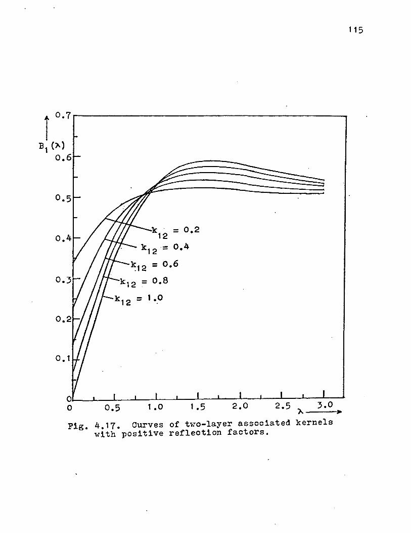
i 0.7

Bl (}.) 0.6

0.5

k 12 = o.4

~12 = 0.6

1 .o

1 .o 1 • 5 2.0 2.5 3.0 '>.--~

Fig. 4.17. Curves of tv-ro-layer associated kernels with positive reflection factors.

115

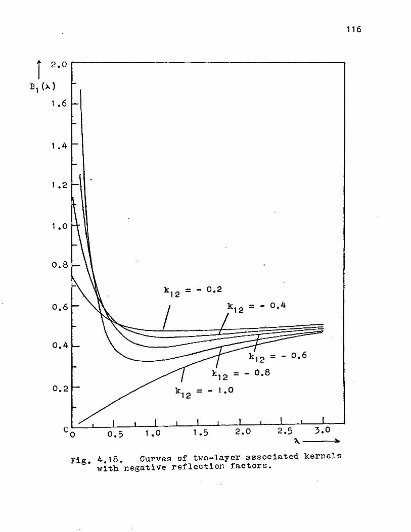
1 2 .o

B1 (:>.)

1 • 6

1 .4

1 .2

1 .o

0.2

= - 0.4

- o.6

-- 1.0

0.5 1 .o 1 • 5 2.0 2.5 3.0

"' )a

Fig. 4.18. Curves of two-layer associated kernels with negative reflection factors.

116

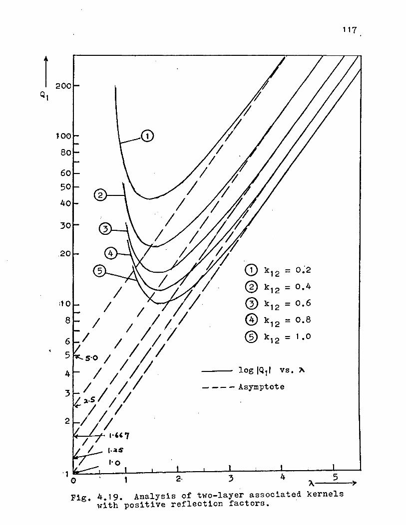
3

2

t-.as

CD k12 = o~2

® k12 = 0.4

® k12 = 0.6

® k12 = 0.8

® k12 = 1 .o

-- log IQ 11 vs. ~

----Asymptote

117

5 "--~

Fig. 4.19. Analysis of two-layer associated kernels with positive reflection factors.

100

80

60

50

40

30

20

10

8

6

5

4

3

2

1 2

118

--_-log fQ 11 vs. 'X

---- Asymptote

3 4 5 X--~)

Fig. 4.20. Analysis of two-layer associated kernels with negative reflection factors.

119

with the two-layer kernel the function logjQ1 j lS not a

linear function of>.. Furthermore one notices that two

different two-layer structures with identical thickness, but

the reflection factors being of opposite signs, are asso

ciated two different log IQ 11 which approach to the same

asymptote at large>.. This common asymptote is represented

by (4.28) and its intersection with the vertical axis depends

only on the absolute value of the reflection factor k 12 .

The layer thickness d1 and the absolute value of the

reflection factor k12

for each two-layer structure are deter

mined from the slope and the intercept of the asymptote

respectively. These determinations can be carried out

graphically by means of a master diagram of the asymptote

similar to the one shown in Fig. 4.5. The correct sign of

k12

cannot be determined from the graph of logjQ1 1 itself.

However, a study of the behavior of Q1 as a function B1 (>.)

will provide the clue to the correct sign of k 12 . From the

definition of Q1

given by (4.27) one observes that Q1 < 0,

B1

(>.) < 0.5; Q1

> 0, 0.5 < B1

(>.) < 1.5; Q1 < 0, B1 (>.) > 1.5;

Q1

~ -ro as B1

(>.) ~ 0.5 -;and Q1

~ +oo as B1 (>.) ~ 0.5 +.

These properties of Q1

are illustrated in Fig. 4.21. Fig.

4.22 shows the curve of an associated kernel for the case

k12

= 1.0 and also the curve of the related function Q1 .

Similar curves for the case k 12 = -0.8 are shown in Fig. 4.23.

We note that in the case with k 12 = 1.0 Q1 is positive beyond

the point of discontinuity and its sign is reversed in the

120

case with k 12 = -0.8. In general it is true that within the

range in which the curve of log!Q1 1 approaches its asymptote,

k 12 will be positive if Q1 is positive and negative if q1

ls

negative.

Next, let us consider the analysis of the associated

kernels of the three-layer case. Figs. 4.24, 4.25, 4.26, and

4.27 are typical examples of the curves of the associated

kernels corresponding to the four groups of resistivity situa

tions in the three-layer case, namely (i) pl < P 2 > p 2 ,

(ii) p1

> p 2 < p3

, (iii) pl > p 2 > p 3 , and (iv) pl < p 2 < p 3 .

It may be noted that curves belonging to each group have a

characteristic shape of their own.

Since the procedure of analysis is identical for all

cases it is suffice for us to consider only the case

P1

: p2

: p3

= 1: 10: l/10 for illustrative purpose. The

results of the analysis is shown in Figs. 4.28, 4.29, 4.30,

and 4.31. The first thing to be noted from these results is

that the curve of logjQ1 j in each case looks almost like that

of the function log!Q1

j obtained from the decomposition of

two-layer associated kernel. Therefore, unlike the analysis

of the kernel, it is not possible to tell from the graph of

log!Q1

1 whether one is dealing with a two-layer problem or

with a more complicated multilayer problem. In order to make

a decision a further step of calculation is needed to be

carried out. This involves the calculation of Ui from (4.33a).

We note that Ui = k 12 in the two-layer problem. Thus if the

121

result of computation indicates that Ui is a constant equal

to k 12 then the structure under consideration is a two-layer,

one. The graph of logjQ 2 j obtained from the second stage of

decomposition is a straight line for each case. ' I Th1s result

is in accordance with that predicted by (4.35). The fact

that the graph of logjQ 2 j 1s a straight line 1n the three

layer case can be used as an indication that no further inhomo-

geneity exists beneath the second boundary plane.

Next, let us study the behaviors of the functions Q1 and

Q2 . The behavior of the function Q1 can readily be examined

from each set of associated kernel curves together with Fig.

4.21 which shows the relation between Q1 and B1 C\). Let us

consider, for instance, the curves of Fig. 4.24. In each

case the function Q1 has two discontinuities because each

curve of the associated kernel intersects the line B1 CA) = 0.5

at two different points. Beyond the second point of inter-

section B1

C\) 1s less than 0.5 in all the four cases, thus

implying that Q1 will be negative beyond the second point of

discontinuity along the \-axis. We note that in this parti-

cular example the reflection factor k 12 is negative because

Thus the sign of k 12 is identical with that of Q1

beyond the second point of discontinuity. Analysis of the

other sets of curves of the associated kernel indicates the

same conclusion.

According to (4.34) the behavior of Q2 is dependent on

K' which is defined by (4.30b). 2

One may note that (4.30b)

r1or---~-----------------------

Q I. 1

I I I I I I I I

-1~--~~~--~--L-~~~---L--~--~--~--~~ 0 3.0

~

122

Fig. 4.21. General relation bet~een the associated kernel and the function Q1 •

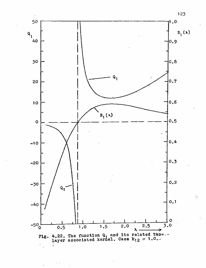
50

0

-10

-20

-30

-40

I I I I I I I I

I I l I I

Q1-- I I I I

1 .o·

-so~~--~~~~~--~~--~~~-L--~~--~o 0 0.5 1.0 1.5 2.0 2.5 3.0

~---~ Fig. 4.22. The function Q1 and its related twoe-

layer associated kernel. Case k 12 = 1.0 •. .:

123

Bl ( ~)

50

Q1 I Q-1

I I I I I I I I I '·

I

I I

:81 ( ") = 0.5 ------

-30

-40

-5o~~~~--~--~--~~--~--~--~~~~--~o 0 0.5 1.0 1.5 2.0 2.5 3.0

A---~

Fig. 4.23. The function Q1 and its related twolayer associated kernel. Case k 12 = - 0.8.

124

.o.

B1 ( ~)

.8

·,

125

2.or-------------------------------------------~

1 .4

1 • 2

dl . d2 =CD 1 • 4 . •

@ 1 • 1i . ® 1 . 2/3 . ® 1 • 1/4 •

0 0.2 0.4 0.8 1 .o 1 • 2 1. 4

~----~

Fig. 4.24. Curves of three-layer associated kernels for the case f. : f.. : f, = 1 : 1 0 : 1 /1 0, :· ; : ·

0.5

0.4

0.3

0.2

o. 1

d1 • d2 =0 •

® Q) @

0 0.2 0.4 0.6 0.8 1 • 0

1 • •

1 • •

1 • •

1 • •

126

4

1i

2/3

1/4

1 • 2 1 .4

"'----~~

Fig. 4.25. curves of three-layer associated kernels for the case f. : {{ : fJ = 1 : 1/1 0 : 1 0.

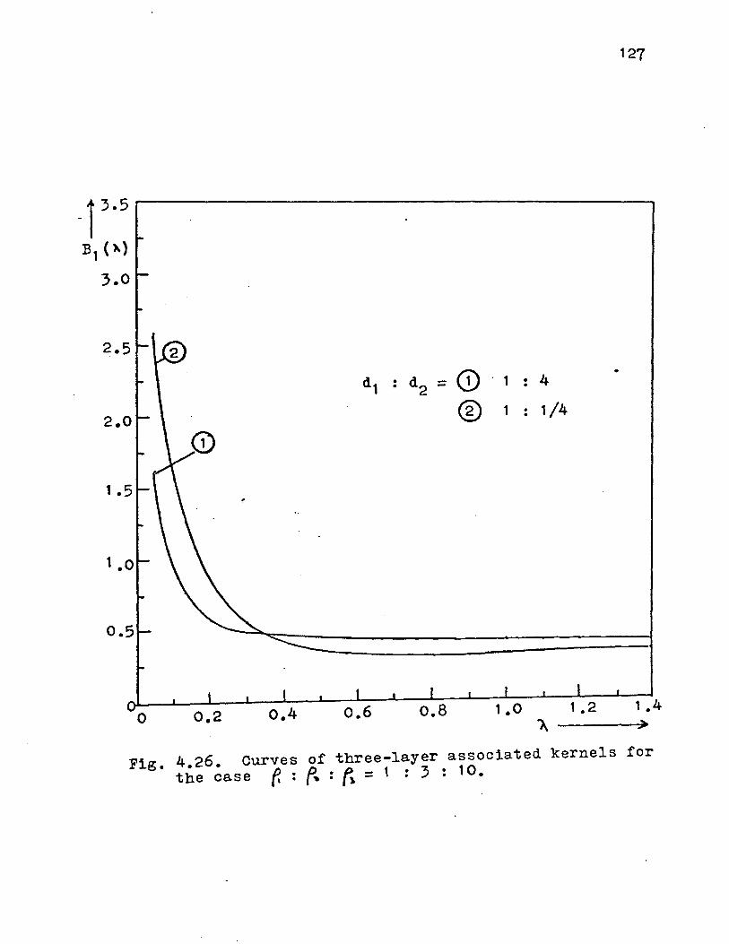
-13.5 131 ().)

0 0.2 o.4

d1 : d2 = 0 . 1 : 4

® 1 : 1/4

0.8 1 .o

127

1 • 2 1 .4 ~ ----~

Fig. 4.26. Curves of three-layer associated kernels for the case f- : ~ : ~ = 1 : 3 : 10.

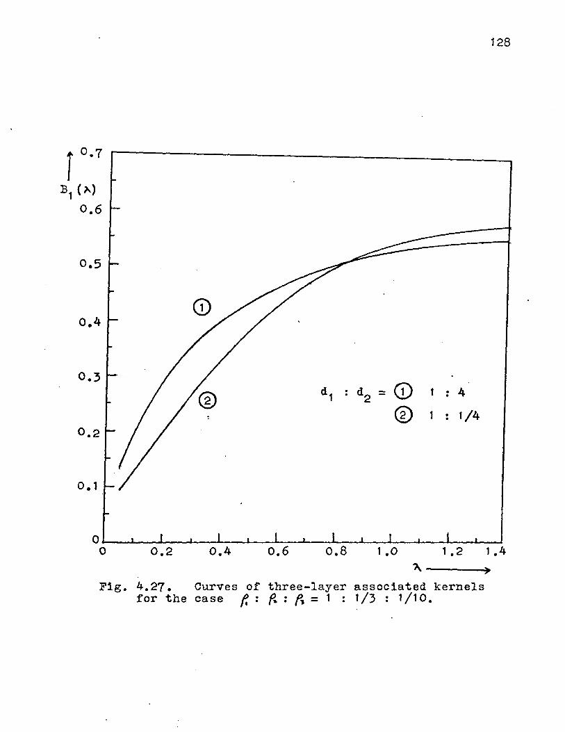
128

0.5

0.4

0.3 d1 .

d2 = CD t . 4 . . ® 1 • 1/4 .

0.2

0.1

0 0 0.2 0.4 0.6 0.8 1 .o 1 • 2 1 .4

~

Fig. 4.27. Curves of three-layer associated kernels for the case f.: {{ : f, = 1 : 1 /3 . 1/10. .

129

200r---------~------------------------------~---

80

60

so 40

30

20

10

8

6

5

4

3

10

..

of logfQ11

I -1 (k12) ~ = 1 • 22

r (k2 a> -1, = 1 • o 1

2 3 4 ).. 5 >

Fig. 4.28. Analysis of three-layer associated kernel of the case f.: ({: fs = 1 : 10 : 1/10, d 1 : d2 = 1 : 4. .

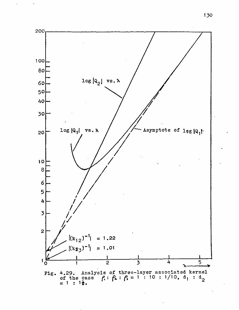
130

200r-----------------------------~----------~~

6

5

2

Fig.

1 og IQ 11 vs • ?\

I

= 1.22

= 1 • 01

1 2 3 4 5 "). .

4.29. Analysis of three-layer associated kernel of the case f.: r~= f, = 1 : 10: 1/10, d1 : d2 = 1 : 1i.

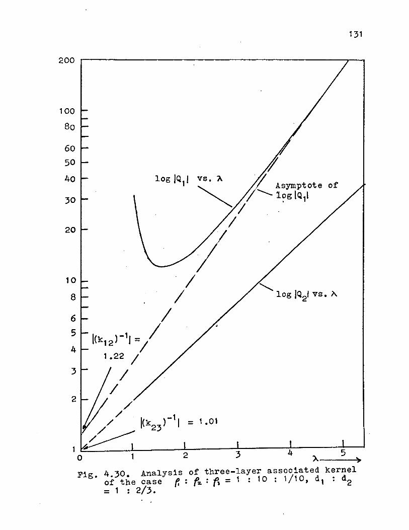
131

200 r---------------~--------------------~--

100

so

60

50

40

30

20

8

6

5

4

3

2

1 • 01

5 A.--~')

Fig. 4.30. Analysis of three-layer associated kernel of the case f.: f-z.: "(l = 1 : 10 : 1/10, d 1 : d 2 = 1 : 2/3.

1000

800

600 500 400

300

200

100 80

60 50 40

30

20

10

8

6 5 4

3 1.22

1 .01

3 4

132

5 ~--~>

Fig. 4.31. Analysis of three-layer associated kernel of the case f.: f ... :f~ = 1: 10: 1/10, d 1 : d2 = 1 : 1/4.

133

is almost identical with the equation for the two-layer

kernel (i.e., equation (4.2)) excepting that 2A has been

replaced by A. From (4.30b) it is evident that K2 is less

than unity if k 23 1s positive and is greater than unity if

k 23 is negative. Thus from (4.34), which is the definition

of Q2 , one can conclude that positive values of Q2 are related

to positive reflection factor while negative values are

related to negative reflection factor.

It may be noted that the thickness d 2 a~d the absolute

value of k23

can be determined with the aid of a suitable

master diagram of the asymptote of Q1 .

Since the analysis of other multilayer problems 1s

exactly identical to that of the three-layer case we shall

not consider further examples. An example of the analysis

of a four-layer case is given in Appendix F.

Alternative Approach to the Analysis of the Kernel: of Logarithmic Curve-Matching

Method

The technique of logarithmic curve-matching is well

known to anyone who is concerned with the direct current res1s-

tivity method of prospecting. This technique was first

developed for the analysis of apparent resistivity curves by

Roman (1940) and is now widely used. The writer finds that

with the aid of the formulas derived for the kernel it is

possible to adopt the logarithmic curve-matching technique

for the analysis of the kernel.

134

The principle of logarithmic curve-matching may be out

lined as follows: Let us consider the two-layer kernel which

is given by (4.2). The kernel may be written implicitly as

The coordinates of a point on the curve of K1

plotted against

Ad 1 are <K 1 , Ad 1 ). In the logarithmic coordinate system the

coordinates of the same point would be (log K1

, logA +log d1

).

Since d 1 is a constant the quantity log d1

is identical for

all points on the curve. If an arbitrary value not equal to

unity is assigned to d1

, then each point on the curve will be

shifted a horizontal distance equal to log d1

with respect

to the corresponding point on the curve for the case d1

= 1.

The shape of a curve plotted in logarithmic coordinates 1s

preserved even when the abscissa of each point along the

curve is multiplied by a constant factor. This preservation

of curve shape in logarithmic coordinates 1s the basis for

the curve-matching method of interpretation. We note that 1n

this particular case of the two-layer kernel the shape of the

curve of the kernel plotted in logarithmic coordinates is

dependent only on the reflection factor k 12 ; two kernel

curves having identical shape will correspond to two different

two-layer structures which have the same reflection factor

but their thicknesses for the first layer may be different.

Before we proceed to discuss the procedure for analyzing

the kernel by means of the curve-matching method let us

135

recall some important properties of the kernel function. In

our earlier analysis it has been shown that the function u1

approaches k 12 at large values of A· This implies that the

kernel K1 CA) of ann-layered structure is reduced essentially

to one of a two-layer case when A becomes very large. Next

we note that the function K. of Equation (4.1) is independent l

of the parameters d. and P· where j = i-1, i-2, i-3, ..... 3, J J

2, l. Considering the three-layer case, for instance, the

function K2

is independent of d 1 and p 1 , and it is identical

to the kernel for a two-layer structure in which the top

layer has a resistivity p2

and thickness d2

, the bottom layer

having a resistivity p 3 and an infinite thickness. From (4.1)

one

.. )

can see that the sequence of functions {K.}, i = 1,2, ... l

n-1, represents a sequence of n-1 layered structures, the

number of layers in each structure being reduced by one as

we go from one member of the sequence to the next member

higher up in the sequence. Furthermore, each member of the

sequence {K.} approaches the kernel of a two-layer structure l

having layer parameters k. '+land d., when A becomes very l,l l

large. The last function K is obviously the kernel of a n-1

two-layer structure.

The curve-matching method involves essentially the

comparison of the curve of an unknown kernel with a master

set of theoretical two-layer kernel curves computed for a

series of different reflection factors, with the thickness

ct1 being assumed to be unity. Figs. 4.32 and 4.33 are

136

examples of such curves. With the aid of the properties of

the kernel function outlined above we can apply the curve

matching method to the decomposition of any multilayer kernel.

The procedure of making analysis may be outlined as follows:

(i) The unknown kernel function lS plotted on a tracing

using bilogarithmic scales which are identical to those used

for the master curves.

(ii) The tracing paper lS then superimposed on the master

diagram. With the abscissa on the tracing paper coinciding

with that of the master curves the overlay is moved horilJ

zontal until a close fit is obtained between the unknown

kernel and one of the theoretical curves.

It lS important to note that if fitting is not possible

for the entire range of A then an attempt should be made to

fit only that portion of the unknown kernel lying in the

upper range of A· In our discussion of the properties of

the kernel we have noted that in multilayer problems the

kernel function will approach asymptotically to the kernel

for a two-layer structure when A becomes large. Thus the

fact that a complete matching between the unknown kernel

and one of the theoretical curves is not possible means that

the unknown kernel represents a structure that has more than

two layers. This accounts for the reason why we should

match only the upper portion of the unknown kernel when a

complete matching is not possible.

137

In the case of complete matching the unknown kernel

represents a two-layer structure which has a reflection fac

tor identical to that of the theoretical curve that fits

the unknown kernel. The thickness d1

is g1ven by the dis-

tance between the origin of the master diagram and the point

at which the vertical axis of the tracing intersects the

abscissa of the master diagram. If the unknown structure and

the theoretical structure have the same thickness, then the

two origins should coincide with each other.

In the case when only partial matching is obtained 1n

the upper range of A we have a multilayer problem.

d1

are still determined in the same way as in the two-layer

case. In order to determine the next set of layer parameters,

namely k23

and d2

, we proceed to the next step of our analy-

SlS.

Cii) Since d1

is now a known quantity it is possible to

calculate u1

and subsequently K2 from (4.18) and (4.19)

respectively by putting i = 2. The resulting values of K2

are then plotted on a tracing paper using bilogarithmic scales.

The matching process is then repeated. If the unknown kernel

represents a three-layer structure then the curve of K2

should match one of the theoretical curves. Fig. 4.34 illus-

trates the analysis of a three-layer kernel for the case

We note that

the curve of K1

CA) fits the theoretical curve with k 12 = -0.8

at its upper range while the curve of K2 matches the theoretical

138

Fig. 4.32. ~aster set of two-layer kernel curves for cases with different reflection factors, logarithmic plotting.

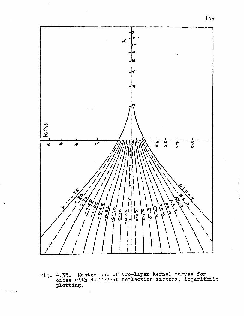
139

Fie. 4.33. }laster set of tlTo-layer kernel curves for cases uith different reflection factors, logarithmic plotting.

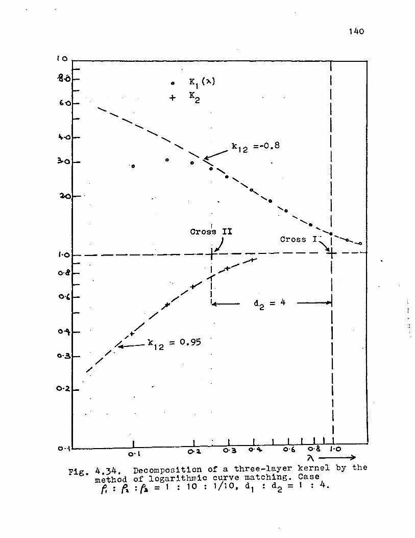
140

ror---------------------------------------~~----

.._ .........

............ .........

............

·o

0

+

I I I

......... " k12 =-0.8

0 '~

I I I

0 """' . 0' ., ' 0......

'•

I I I

r ',• I Cross II '-•

·) Cross I\1-'-o_-o ----------J!-------- ~--. ,.....,..... I

. I ,+"' ¥i I

/ I ?'/ 'o( d2 - 4 ~I

// I /+ I

~ _ k 1 2 - o. 95 I /·

/ /. I I I I l I

Pig. 4.34. Decomposition of a three-layer kernel by the method of logarithmic curve matching. Case r. = fa = r~ = 1 = 1 o = 1 11 o, d 1 = d 2 = 1 = 4.

141

10.---------------------------------------r----------

0·'

+ K' 2

- - 0.8

I I I I I I I I I I

' .2 I ' ~d = 3 ~I + :-- ........... , 1 d = 2 ---1

+ +'I · 1 3 1 Cross I

,=~="- :.---.! '/

+

---------- /+-- 1~ .. :;;--;-s~II~---~-/ ;'/Y' .--1

Cross II _, IY' ~_...-

o 0/~ ~ I 0 0 0 #,.....,.. '\

• -;,A k = o.s I ---~¥" 12 1

-------- / I -- -~

0.95

o· l 0·~ 0·~ 0·'

I I I I I I I I

I 1·0

'A )

Fig. 4.35. Decomposi t1on of a four-layer kernel by the method of loearithrnic curve matching. Case

f,: fi:~ :f,.= 1: 1/3 : 3 : 1 /1 0, d1 . d2 . d3 . . = 1 . 3 • 2. • .

-o

142

lOr-----------------------------------------~---------

' Cross Cross 'o III II '-.....o

) / 1'-o -o

1·0 ---------¥--~--~-~--~~ f'A-A 1 -+- - 1'" k 12 = 0.5 _ ... A-1 ~-.....- Cross I

~ A--A --1~ I I .,A - ,.. ,.... ,......, t . I

-' ,--+ 1 . L I ,..- """ d 2 --+ ...... ~ .- + I 2= I

-- .-'· I --_, + '· d3 = 3 _J 0·,. - ,..........

+ k1 2 = 0.55 I

- ,.!... •

...

A K 3

I I I I I I

. . .

4.36. Decomposition of a four-layer kernel by the method of logarithmic curve matching. Case f, : fa. : ~ : f,. = 1 : 1 0 : 3 : 1 , d 1 : d2 : d3

= 1 : 2 : 3.

143

curve with k 12 = 0.95 completely. The crosses I and II are

the positions of the origin of the master diagram for the

first and second matchings respectively. From the positions

of these crosses one finds that d1

= 1 and d2

= 4.

If only partial matching of the curve of K2

is obtained

this indicates the existence of a deeper layer (or layers).

It is necessary to carry out the matching one step further

by computing the functions U2 and K2 respectively from (4.18)

and (4.19) with i = 3. Figs. 4.35 and 4.36 illustrate the

analysis of two typical four-layer kernels.

(iv) In general the process of decomposing the kernel is

considered to be completed if a complete match is obtained

for the curve of K .. l

Limits of Solubility

In the study of apparent resistivity curves one may

encounter the fact that certain three-layer resistivity situa-

tions, nominally quite different, have apparent resistivity

curves which are identical to a first approximation. This

problem is found to be associated with the cases of thin

intermediate layers of resistivity either much higher or

lower than that of the top and bottom layers. Explanation

for this phenomenon may be obtained by examining the kernel

function.

The three-layer kernel is expressed analytically by

(4.9a). The function u1

appearing in (4.9a) may be written

out explicitly ln the form

= (pl- p2)(p2 + p3) + (pl + p2)(p2

(pl + p2)(p2 + p3) + (pl- p2)(p2

144

When the thickness of the intermediate layer is assumed to be

. -2Ad so thln that e 2 (1 - 2Ad 2 ) the above expression for u1

may be written as

(pl - p2)(p2 + p 3) + (pl + p2)(p2 - p 3) ( 1 - 2Ad2) ul =

(pl + p2)(p2 + p 3) + (p - p2)(p2 - p3)(1 - 2Ad2) 1

( p 1 + p 2) ( p 2 - p 3)

1 3 p2 p 2 A p 2 d2

= (4.41) (pl - p 2) ( p 2 - p 3)

+ Ap2 d2 1 3 p 2 p 2

When the resistivity of the intermediate layer is very high,

compared to pl and p 3 , we have a further approximation as

follows:

On the other

lS very low,

ul

p 1 - p 3 - A p 2 d2

pl + P3 + Ap2d2

hand, when the resistivity of

compared to pl and p 3' (4.41)

pl - p 3 + Aplp3 (d2/p2) = (d2/p2) pl + p 3 - A p lp 3

(4.42)

the second layer

lS reduced to

(4.43)

145

When the values of d2

and o2

are such that c 1 or c 2 is a constant in all cases, this leads

to the phenomenon that different three-layer resistivity

situations have identical kernel to a first approximation,

and thus identical apparent resistivity function also. Under

such condition it is extremely difficult to distinguish any

two cases that have identical cl or c2.

blem seldom arises as such in practice.

Fortunately the pro-

The problem of detecting a thin second layer still exists

even though the resistivity of this layer does not belong to

either one of the two extreme cases mentioned above.

consider two cases, the first of two layers

pl = l dl = l

p 2 = 3 d2 = 00

and the second of three layers

pl = l dl = l

p 2 = 10 d2 = 1/10

p 3 d3 = 00

= 3

Let us

The values of the kernels corresponding to these cases are

given in Table 4.1. Examination of these values shows that

only a small difference exists between the value of the

three-layer kernel and that of the two-layer kernel. In

146

TABLE 4.1 Comparison of a tHo-layer kernel uith two three-layer kernels associated with the case of thin intermediate layer

I II III

0.02 2.8491 2.8652 3.0261

0.04 2.7144 2.7433 3.0280 - .

0.06 2.5936 2.6325 .3.0100

o.o8 2.4848 2.5315 2.9763

0.10 2.3862 2.4391 2.9305

0.20 2.0082 2.0753 2.6157

0.40 1 .5795 1. 6427 2.0159

0.60 . 1 .3546 1 • 4050 1. 6344

0.80 1. 2246 1 • 2628 1 .4042

1 .oo 1 • 1452 1 ·. 1736 1 .2622

I. two-layer kernel with reflection factor .k12 = -0.5

II. three-layer kernel for the case f. : f,. : ~ =

1 : 1 o : 3, d 1 : d2 · = 1 : 1 I 1 o III. three-layer kernel :for the case · f. : {{ : {{ -

1 : 1 00 : 3 t d 1 : d2 = 1 : 1 /1 0

the last chapter we have shown that the deviations of the

values of the kernel integrated from apparent resistivity

data from its theoretical values are almost of the same

147

order of magnitude. Thus it will be very difficult to detect

the presence of a thin second layer by analyzing the kernel

function, even when the resistivity of the second layer is

10 times greater than that of the surface layer. The increase

1n resistivity contrast may improve the resolving power of

the kernel function associated with a thin second layer.

This 1s evident by examining the values of the kernel for the

case p2

= 100 as shown in Table 4.1.

Further examples which illustrate the difficulty involved

1n distinguishing a three-layer kernel associated with a thin

second layer from that of a two-layer case are shown in Figs.

4 . 9 and 4 .I 0 . The dash curves shown on these figures are

curves of two-layer kernels. In Fig. 4.10 we can see that

when the thickness d2

of the intermediate layer is only ~

that of the surface layer the three-layer kernel deviates only

slightly from the two-layer kernel. The distinction between

the two kernels is even worse 1n the case shown in Fig. 4.9.

In general one may conclude that the resolving power of

the kernel is dependent both on the resistivity contrast and

the relative thickness of the intermediate layer. The ability

to distinguish between two nearly identical cases is limited

by the accuracy of the data.

CHAPTER V

SUMMARY AND CONCLUSION

148

This investigation was primarily concerned with the

interpretation of resistivity sounding data measured by the

Wenner electrode system. More specifically, there were two

maln objectives: (i) to derive from the apparent resistivity

data directly some functions from which the resistivity and

thickness of each member of the sequence of layers composing

the earth might be determined, and (ii) to devise suitable

methods for the analysis of the resulting functions.

In this study it was assumed that the earth might be

approximated by an n-layer model. It was shown that the

solution of the boundary value problem associated with the

model of an n-layer earth led to an integral equation for

the Wenner electrode system. This integral equation relates

the apparent resistivity function to an unknown function,

termed the kernel, which depends on the layer resistivities

and thicknesses. A solution of this integral equation was

obtained by the use of a Hankel transform. The solution did

not give rise to the kernel directly, but rather to a related

function, termed the associated kernel. A simple relation

exists between the kernel and the associated kernel and this

is given by (2.20). From the associated kernel it was

possible to derive an explicit integral expression of the

kernel in terms of the known apparent resistivity function.

149

Numerical integration formulas based on the Legendre

Gauss quadrature formula were developed for the calculation

of the kernel and the associated kernel respectively from

apparent resistivity data. Since the apparent resistivity

function is generally known only at a certain number of

electrode separations by direct field observation, a method

for generating unknown values of the apparent resistivity

function from the known data is necessary because the process

of integration requires a knowledge of the apparent resis

tivity function at points other than those input data points.

It was found that the unknown values could be generated quite

satisfactorily by the method of least-squares approximation

using orthogonal polynomials obtained by Forsythe's method.

Results of numerical integration show that there was close

agreement between the integrated values of both the kernel

and the associated kernel and their respective theoretical

values.

It ls of importance to note that in order to take care

of the oscillating nature of the integrands associated with

the integrals of both the kernel and the associated kernel

it was necessary to divide the interval of integration into a

number of subintervals so that the integrand of each integral

might be sampled accurately. The choice of the number of

subintervals is dependent on the parameter A; generally the

larger the value of A the greater the number of subintervals

will be needed. When a very large number of subintervals is

150

used the roundoff errors ln the quadrature formulas may

become a serious problem. So this appears to be the limita

tion on the use of the numerical integration formulas

developed in this investigation. Fortunately in the course

of analyzing the kernel and the associated kernel it was

found that the values of these functions which are of interest

for the determination of layer resistivities and thicknesses

were associated with those values of A lying within a small

range (0,5). Within this range of A we had obtained satis

factory results with the integration formulas.

In practice, apart from the errors inherent ln the inte

gration formulas, several other factors may influence the

results of integration. These factors are (i) inaccuracy ln

the measurement of the apparent resistivity data, (ii) error

in the least-squares approximation, (iii) uncertainty asso

ciated with the determination of a and b, and (iv) error in

the measurement of pl and Pn·

Two methods were developed for the determination of

layer resistivities and thicknesses. The first one is the

numerical-graphical method which can be used for the analysis

of both the kernel and the associated kernel. The other

method which was developed mainly for the decomposition of

the kernel is the method of logarithmic curve-matching. In

practice, the numerical-graphical method may suffer two

disadvantages: (i) there is not much latitude in the choice

of the slope of the asymptote, and (ii) for large values of

151

thickness the intersection of the asymptote with the ordinate

axis may not be very sharply defined due to steep slopes.

These disadvantages may be partially offset by varying the

scale of either the abscissa or the ordinate. The logarithmic

curve-matching method does not possess these disadvantages.

The problem of detecting a thin intermediate layer 1n

the three-layer case was considered. It was shown that unless

a great contrast in resistivity exists the ability to detect

the presence of a thin second layer is limited by the accuracy

of the data.

152

REFERENCES

Bowman, Frank, 1958, Introduction to Bessel Functions: New York, Dover Publications, Inc., l35p.

Forsythe, G. E., 1957, Generation and use of orthogonal polynomials for data fitting with a digital computer: Journ. Soc. Indust. Appl. Math., V. 5, No. 2, p. 74-87.

Grant, F. S., and West, G. F., 1965, Interpretation theory in applied geophysics: New York, McGraw-Hill, 583p.

Hildebrand, F. B., 1956, Introduction to numerical analysis: New York, McGraw-Hill, 5llp.

Kaplan, Wilfred, 1952, Advanced calculus: Wesley, 679p.

Reading, Addison-

Keller, G. V., and Frischknecht, F. C., 1966, Electrical methods in geophysical prospecting: New York, Pergamon Press, 517p.

Koefoed, 0., 1965, Direct methods of interpreting resistivity observations: Geophysical Prospecting, V. 13, No. 4, p. 568- 592.

----, 1966, The direct interpretation of resistivity observations made with a Wenner electrode configuration: Geophysical Prospecting, V. 14, No. 1, p. 71 - 79.

Langer, R. E., 1933, An inverse problem in differential equations: Am. Math. Soc. Bull., V. 39, p. 814- 820.

Oliver, F. W. J., 1965, Bessel function of integer order, 1n Handbook of Mathematical Functions: New York, Dover Publications, Inc., 1046p.

Mooney, H. M., and Wetzel, W. W., 1956, The potentials about a point electrode and apparent resistivity curves for a two-, three-, and four-layer earth: Minneapolis, University of Minnesota Press, l46p. and 243 loose sheets of reference curves.

Pckeris, C. L., 1940, Direct method of interpretation in resistivity prospecting: Geophysics, V. 5, No. 1, p. 31- 42.

153

Paul, M._K.? ~968, A ~ote on the direct interpretation of r~s1st1v1ty pr?flles for Wenner electrode configuratlon: Geophys1cal Prospecting, V. 16, No. 1, p. 159 -162.

Ralston, Anthony, 1965, A first course in numerical analysis: New York, McGraw-Hill, 578p.

Roman, Irwin, 1940, Superposition in the interpretation of two-layer earth resistivity curves: U. S. Geol. Survey Bull. 927-A, l8p.

________ , 1960, Apparent resistivity of a single uniform overburden: U. S. Geol. Survey Prof. Paper 356, 99p.

Scott, E. J., 1955, Transform calculus: and Row, 330p.

New York, Harper

Slichter, L. B., 1933, The interpretation of the resistivity prospecting method for horizontal structure: Physics, V. 4, p. 307 - 322.

Sneddon, Ian N., 1951, Fouries transform: New York, McGraw-Hill, 542p.

, 1955, Functional analysis, in Encyclopedia of ------~-Physics, V. 2: Berlin, Springer-Verlag, p. 198 - 347.

Stroud, A. H., and Secrest, Don, 1966, Gaussian quadrature formulas: New Jersey, Prentice Hall, Inc., 374p.

Sunde, Earling D., 1949, Earth conduction effects in transmission systems: Princeton, D. Van Nostrand, 370p.

Van Nostrand, R. G., and Cook, K. L., 1966, Interpretation of resistivity data: U. S. Geol. Survey Prof. Paper 499, 310p.

Vozoff, Keeva, 1956, Numerical resistivity analysis: sics, V. 23, No. 3, p. 536 - 556.

Geophy-

154

APPENDIX A

CONCEPT OF APPARENT RESISTIVITY

The potential about a point current electrode located

on the surface of a homogeneous ground of resistivity p l

(Fig. A.l) is given by the equation

where R is the distance from the current electrode and I is

the current introduced into the ground by the electrode.

Suppose that we have a general four-electrode configuration

located on the surface of the ground as shown in Fig. A.2.

A potential difference of ~V volts exists between the poten

tial electrodes P1 and P2 when a direct current of I amperes

flows between the current electrodes c1

and c2 . This poten

tial difference ~V can readily be calculated by uslng (A.l).

We note that since the potential function V is a scalar, then

by the principle of superposition the potential at any point

due to a number of current sources lS simply equal to the

sum of the potential contributions from each individual

current source considered independently. Thus

(A.2)

where

Point current /electrode

J

I '\\R I \ , 1 homogeneous ' 1 ..a(/ earth ' / -i--

1 J ~ z

Fig. A.1. Point current electrode on surface of homogeneous earth.

Fig. A.2. A general four-electrode configuration

01

Fig. A.3. The 1·Tenner configuration

155

f = {-1-Rll

1

R21 1 + _1_}

Rl2 R22

156

The function f which lS generally known as the 'form factor'

is clearly dependent only on the geometry of the electrode

configuration. In practice the four electrodes are usually

arranged along a straight line and there are many ways of

positioning the potential electrodes with respect to the

positions of the current electrodes. One of the most widely

used configuration is the Wenner system as shown in Fig. A.3.

In this configuration the electrodes are spaced at an equal

distance t apart. The form factor f of this particular sys-

tern takes a very simple form f = 1/t. It follows that the

potential difference between P1 and P2 is given by

t:N = Ip1/2nt. (A.4)

Since only the Wenner configuration will be considered in

this thesis we shall not describe the other electrode con-

figurations here. The description of other electrode systems

can be found in many references (e.g., Grant and West, 1965).

If the ground is completely homogeneous (A.4) can be

used to calculate the true resistivity of the ground when

measurements are made with the Wenner electrode configuration.

If the ground is inhomogeneous then (A.4) is used as a definition

for the 'apparent resistivity' of the ground -- the res1s-

tivity which the ground would have if it were homogeneous.

By letting pa to denote the apparent resistivity, it follows

157

from (A.4) that

Pa = 2nt !N T (A.S)

The apparent resistivity may bear no relation to any actual

value of the resistivity in the inhomogeneous ground. It

usually falls within the range of the true resistivities of

the materials within the ground over which the measurements

are made.

158

APPENDIX B

SOLUTION OF LAPLACE'S EQUATION IN THE N-LAYER CASE

The Laplace's equation

1 av r 'dr = 0 ( B .1)

which was derived in Chapter II can be solved by the well

known oethod of separation of variables. By assuming that

V(r,z) = F(r)G(z) in which F(r) is a function of r only and

G(z) is a function of z only, (B.l) can be reduced to the

following two ordinary differential equations:

(B. 2)

and

(B. 3)

where A is the separation constant. The two linearly inde-

pendent solutions of (B.2) are eAZ and e-AZ while the two

linearly independent solutions to (8.3) are the Bessel func-

tions of zero order, namely J 0 (Ar) an~ Y0 (Ar).

We note that Y0

(Ar) has a logarithmic singularity at

r = 0. Since the potential function V(r,z) must be continuous

along the positive z-axis except at the origin where the

current source is located, the solution which contains

Y0 CAr) is not acceptable. The general solution to (B.l)

which is obtained by linear superposition of terms of two

types, namely J 0 CAr) eAZ and J0

CAt) e-Az, is glven by

159

V ( r , z ) = f ~( A 0 ) e- A 2 + 8 0 ) e A z) J 0

( At ) d A. (B.4)

0

where A(A) and B(A) are arbitrary functions of A.

Next, we note that the function,

where R = Cr2 + z 2 )~, lS also a solution of Laplace's equa-

tion. One immediately recognizes the fact that the function

V lS actually the potential about a point current source in p

a homogeneous medium. It is obvious that the sum of VCr,z)

and V lS a solution of Laplace's equation. p

write the solution to (2.11) as

0

Thus we may

(B. 5)

where i = 1 , 2 , 3 , ..... , n . The inclusion of V into the solup

tion makes the potential function V1 satisfy the condition

near the current source automatically.

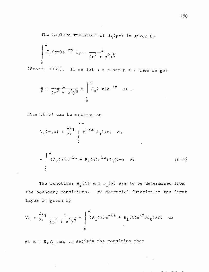
The Laplace transform of J0

(pr) 1s g1ven by

JooJO(pr)e-sp dp =

0

1

+ s 2) ~

(Scott, 1955). If we let s = z and p = A then we get

1 1 J OOJ 0 ( r)e -AZ R = = dA 2 2 1:: .

(r + z ) 2

0

Thus (B. 5) can be written as

V.(r,z) Ipl J ooe-AZ J

0(Ar) dA = ~ l

0

+ I co( Ai ( ' ) e- A z + B ( ' ) A 'Z) J ( ) 1\ i 1\ e . 0 Ar dA

0

160

(B. 6)

The functions A.(A) and B.(A) are to be determined from l l

the boundary conditions. The potential function in the first

layer is given by

dA

0

At z = o>v1

has to satisfy the condition that

161

dvlj -az z = 0 = 0.

This condition can be satisfied if A1

(A) = B1

(A). Thus the

above expression for vl is reduced to

Ipl vl = J -e -Az J 0 (Ar)dA + I -Al (A )(e -Az AZ

21T + e )J 0 <Ar) dA

0 0 (8.7)

By considering the boundary condition that V (r,z) + 0 as n

z ~oo, one can see that the function Bn(A) which appears 1n

the integral expression of V must vanish. Thus n

v n dA (B. 8)

Next, we will consider the conditions of continuity of the

potential and of the normal component of current density at

each boundary plane. The application of the condition of

continuity of the potential to (8.7), (8.6), and (8.8),

respectively leads to the following set of equations:

=A (') -A:Z.. + B ( ) AZ. i+l A e 1 i+l A e 1

(8.9)

where 1 = 2, 3, ..... ,n-2.

162

Another set of equatl"ons ls bt · d f h o alne rom t e condition of

continuity of normal component of current density:

-)..z. 'Z 'Z {-ce l- A.(J.)e-A i + B.(J.)eA i} l l

{ -)..Z -)..z >..z -ce n-1- An_ 1 CJ.)e n-1 + Bn_ 1 (>..)e n-1} =

pn-1 -AZ -I.Z {-ce n-1- A (>.)e n-1}

n

where c = Ip1

/211.

By solving the above two sets of equations one can

(B.lO)

determine all the A(J.) and B(J.). Since only the potential v1

is of interest to us it is not necessary to solve for all the

unknown functions of>. except A1 CJ.).

For example, by solving the equations for the two- and

three-layer cases respectively, we obtain the following

results:

(i) Two-layer case

l+k -2>..dl 12e

(ii) Three-layer case

where

and

( 1 -

163

(B. 11 )

(B.12)

The quantitits k12

and k 23 are called the reflection factors

which have the general form ki,i+l = (pi- Pi+l)/(pi + Pi+l).

It may also be noted that z1 = d1 and z 2 = d 1 + d 2 (see Fig.

2 .1) .

By substituting (8.10) or (8.11) into (B.7) and then

putting z = 0 we obtain the potential on the ground surface

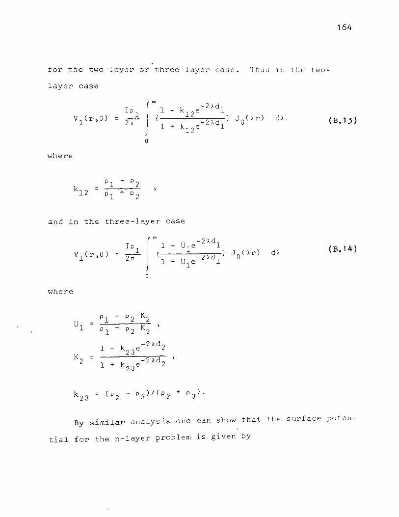
164

for the two-layer or three-layer case. 1'h u:J ln thC' two-

layer case

d>. (B.13)

0

where

and ln the three-layer case

d>. (B.14)

0

where

pl - p2 K2 ul =

pl + p2 K2 '

1 - k -2>.d2 23e

K2 = k -2>.d2 ' 1 + 23e

By similar analysis one can show that the surface paten-

tial for the n-layer problem is given by

Ipl r: - U e- 2 >-dl V1 Cr,O) = ~

1 } Jo(>-r) d>. + Ule-2ndl

0

where

. . . . . . . . . . . . . . . . . . . . . . . ......... .

. . . . . . . . . . . . . . . . . . . . . . . . . . . . . . . . .

K = (1 - U e- 2'-dn-1)/(1 + U e- 2 '-dn-1) n-1 n-1 n-1

u n-1 = k n-l,n = (p 1- p )/(p 1 + p ). n- n n- n

165

(B.15)

(B.15a)

Let K1

Ct.) denote the bracketed quantity under the integral

slgn of (8.14). Then the general expression for the poten-

tial function takes the form

166

d>. (B. 1 6)

This form of the potential function was originally derived by

Sunde (1949), but is seldom encountered in the literature.

The writer finds that the function K1 C>.) is a very convenient

formula for the determination of the layer resistivities and

thicknesses. The method for analyzing K1 C>.) will be pre

sented in Chapter IV.

It may be noted that the potential function is often

written as

V1 Cr,O) = d>. )

(B. 17)

particularly in the European literatures (e.g., Koefoed,

1965). The function A1

C>.) is called the Slichter's kernel.

In our discussions we reserve the term 'kernel' for the

function K1 C>.) only.

APPENDIX C

SOME PROPERTIES OF THE FUNCTION F(At)

The function f(At) which is defined by the infinite

series (2.18) may be written in the form

F(x) = J 0 (x) + f(x)

where

f( x) =

and

X = J..t.

167

(c. l)

(c. 2)

To test the convergence of f(x) let us compare it with

an infinite ser1es of constants

00

S = E 112 2k (c. 3)

k=l

The infinite ser1es S can easily be shown to converge abso-

lutely. By comparing then term of (C.2) with that of (C.3)

it is obvious that

1 n - J 0 Cx/2 ) 2

2n 1

< --- 2n 2

for all x where 0 < x < oo, Thus according to Weierstrass M

test for uniform convergence, the series f(x) converges

168

absolutely for each x and is uniformly convergent in the

interval ( 0 ,oo). Since both J 0 Cx) and f(x) are convergent

it follows that their sum F(x) must also be convergent.

Next, we will consider the calculation of the series

f( X) . Since f(x) is a convergent series approximate values

of f(x) may be obtained by truncating the series after an

appropriate number, say N, of terms. So the question now

lS to determine N such that the truncated series would give

us the values of f(x) to the desirable degree of accuracy.

f(x) may be written as

f( x) = P + Q n n

where P lS the partial sum of the first n terms of the n

series and Q is the remainder. n

We want to find an N(€) such

that

< € for n > N(€)

where E is some small positive number. Since f(x) is a con-

vergent series we can find a sequence Tn converging to zero

for which

< T n

for n > n 1 .

T · notone decreasing then we can choose If the sequence n lS mo

N(£) as the smallest integer after which Tn < £. For if

N(£) lS so chosen and n ~ N(£), then

169

Kaplan (1952) shows that if a series converges by the compari-

son test, then the remainder is in absolute value at most

equal to that of the comparison series. Thus if we let T n

denote the remainder of (C.3) it can be shown that

T = 1 I 3 ( 2 ) 2 n n

It follows that

1 <

3 (2)2n

Hence the upper bound of the error introduced by truncating . -2n

the series f(x) after the first n terms is £ = 1/3 (2) .

If £ is given then N(E) can be found from

N(E) = -(log E + log 3)/log 4.

From (C.l) we can see that the approximate value of F(x)

is given by

F(x) N (E)

= J0(x) + I

k=l

1 k -2k Jo(x/ 2 ) 2

N(E)

= l: k=l

1 k -- J0

(x/2 ) 22k

(c. 4)

(c. 5)

It may be noted that the calculation of F(x) involves

the evaluation of the Bessel function of first kind of zero

170

order which lS defined by the infinite serles

00 (-l)k 2k L: { ~}

k=O (k!) 2 2

This series representation of J 0 (z) is not suitable for

numerical calculations when the values of z is large, say

10 or greater. The writer finds that the polynomial approx-

imations of J 0 (z) presented by Oliver (1965) are more suitable

for computational purposes than the original infinite serles.

An outline of these polynomial approximations is given below:

For 0 < z < 3

J0

(z) = 1 - 2.2499997(z/3) 2 + 1.2656208(z/3)4

0.3163866(z/3) 6 + 0.0444479(z/3) 8

- 0.0039444(z/3) 10 + 0.0002100(z/3)12

+ £

For 3 < z < oo

where

k J

0(z) = f cosY I (z) 2

f = 0.79788456 - 0.00000077(3/z) - 0.00552740(3/z)2

(c. 6)

(c. 7)

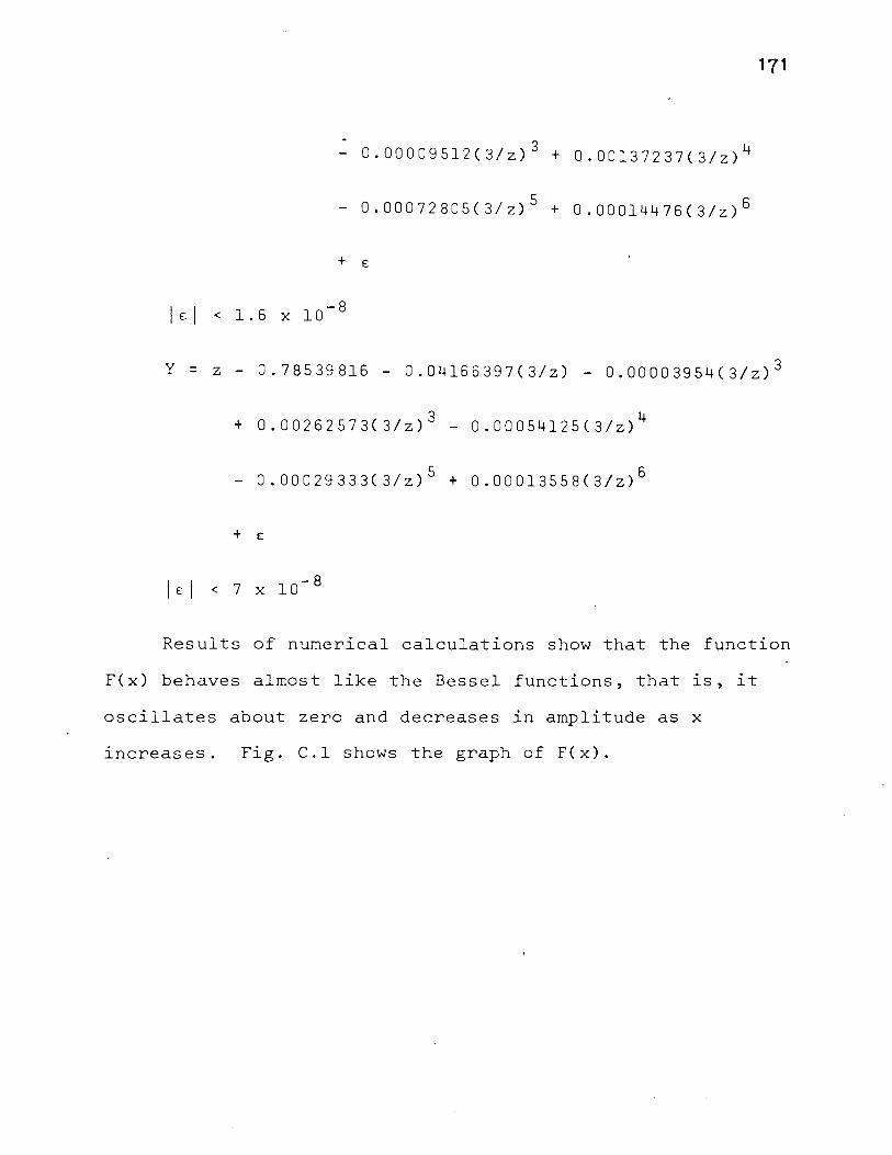
- 0.00009512(3/z) 3 + 0.00137237(3/z) 4

- 0.00072805(3/z) 5 + 0.00014476(3/z) 6

+ E

-8 < 1.6 X 10

171

Y = z - 0.78539816 - 0.04166397(3/z) - 0.00003954(3/z) 3

+ 0.00262573(3/z) 3 - 0.00054125(3/z) 4

- 0.00029333(3/z) 5 + 0.00013558(3/z) 6

+ E

Results of numerical calculations show that the function

F(x) behaves almost like the Bessel functions, that 1s, it

oscillates about zero and decreases in amplitude as x

increases. Fig. C.l shows the graph of F(x).

172

~ Q

0 . -II) 0 0 I •

Fig. 0.1. Graph of the function F(x) oo1

= Z: 2kJo(x/2k) kCO 2

173

APPENDIX D

LAGRANGIAN INTERPOLATING FORMULAS

Suppose that the apparent resistivity function p (t) is a

known at n+l points t 0 , t 1 , t 2 , ..... , tn' which may or may

not be equally spaced. It can be shown that the Lagrangian

approximation to p (t) is given by a

where

p ( t) -a

n L: lk(t) Pa.Ctk)

k=O ( D .1)

t ) n

(Hildebrand, 1956). When n = 2 we have the coefficients of

the three-point interpolating formula given by

When the three points are equally spaced the above coeffi-

cients can be reduced to a more convenient form for computa-

tion by a change of variable

t = t 0 + sh

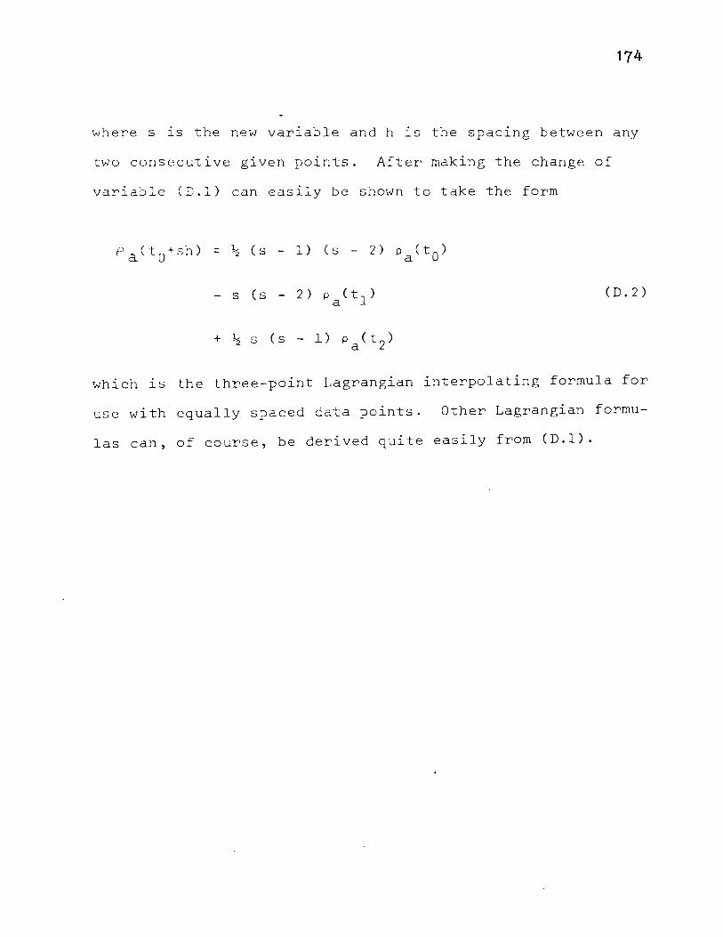
174

where s lS the new variable and h is the spacing between any

two consecutive given points. After making the change of

variable CD.l) can easily be shown to take the form

P act 0 +sh) = ~ Cs - 1) Cs - 2) paCt 0 )

- s (s - 2) paCt 1 )

+ ~ s (s - 1) pa(t 2 )

(D. 2)

which is the three-point Lagrangian interpolating formula for

use with equally spaced data points. Other Lagrangian formu

las can, of course, be derived quite easily from (D.l).

175

APPENDIX E

COMPUTER FLOW DIAGRAMS FOR LEAST-SQUARES APFROXll~TION

AND FOR CALCULATION OF THE KERNEL AND

ASSOCIATED KERNEL

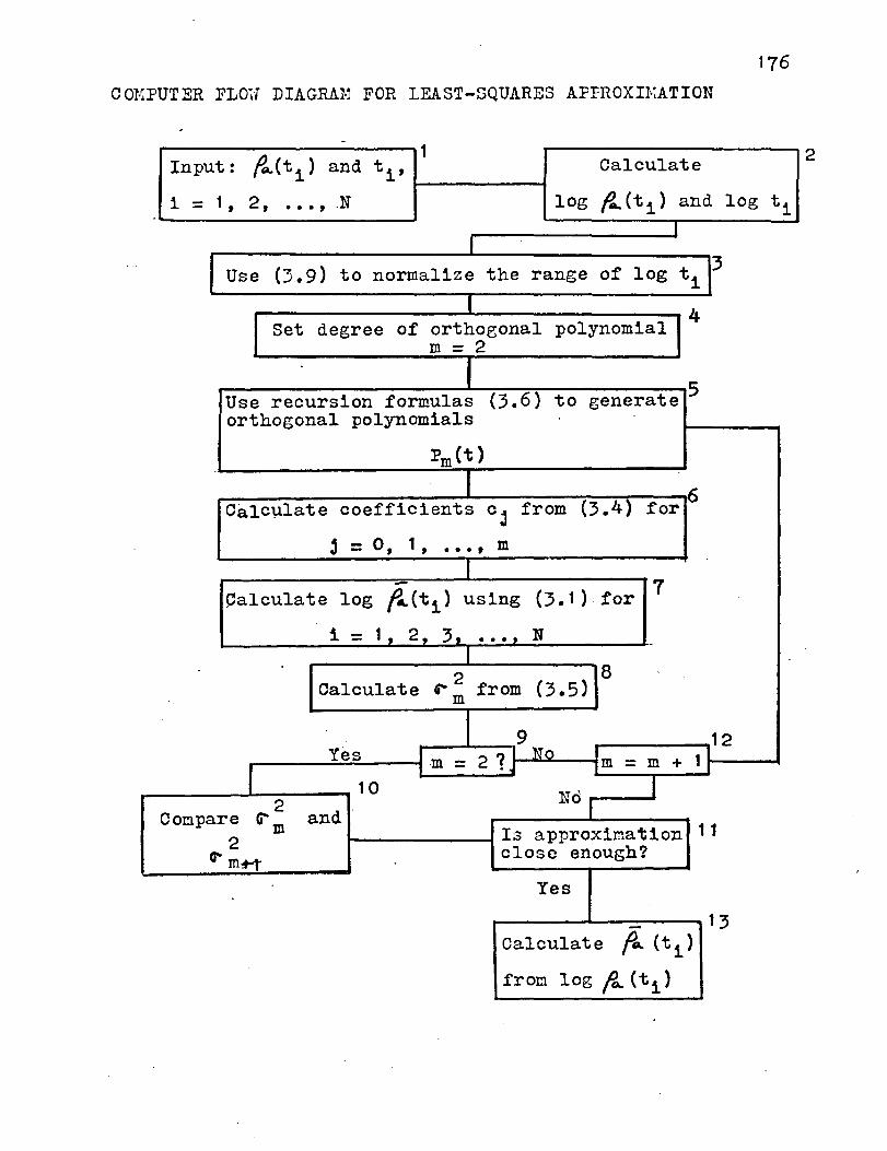
176

C01-iPUTER FLO.J DIAGRA:H FOR LEAST-SQUARES AFFROXII>:ATION

~(ti) and 1

Input: ti, Calculate 2

i = 1, 2, • • • ' .N log fa_(ti) and log ti

I

Use (3.9) to normalize the range of log t1 13

I 4 Set degree of orthogonal polynomial

m- 2

I generate 5

Use recursion formulas (3.6) to orthogonal polynomials

Pm(t)

I ~

CalC\llate coefficients cj from (3.4) for !""'

j = o, 1 ' •• • ' m I - 7 Calculate log f,t(ti) using (3. 1 ) .for

1 = 1, 2, 3, . . . ' N -I

2 8 Calculate a-m from (3.5)

I 9 12 Yes '-m = 2 ? J No {m 1 I

r I = m + 10 No r

2 Compare G"'m and-

Is approximation 1 1 2

~ m:t-t close enough?

Yes

13 Calculate fo. (ti)

from log fa- (ti)

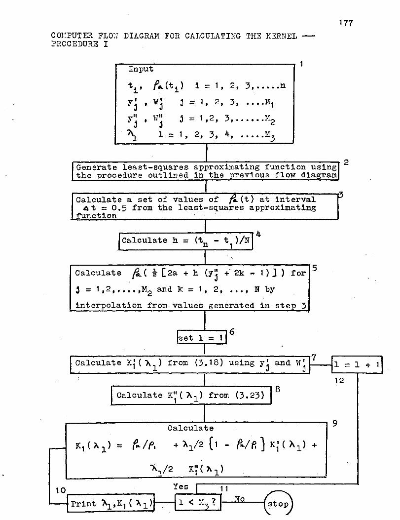
COl:PUTER FL0~1 DIAGRAM FOR CAJ,CULATING THE KERNEL -PROCEDURE I

-Input 1

ti, ~A.(ti) i = 1 , 2, 3, ••••• h

y' j

, W' j j - 1 , 2, 3, •••• 1·11

y" j

, 1'111

j j = 1 , 2' 3, .••••• M2

"\ 1 = 1 , 2, 3, 4, ••••• M3

177

Generate least-squares approximating function using 2

the procedure outlined in the previous flow diagram

-Calculate a set of values o! ~(t) at interval 1-.1

4 t = 0.5 from the least-squares approximating :function

_lcalculate h - (tn - t1 )/Nl4

Calculate ~( t [2a + h (Yj +. 2k - 1) J ) for 5

j = 1,2, •••• ,M2 and k = 1, 2, . . . ' N by

interpolation from values generated in step 3

~et 1 = d 6

7 Calculate Ki ( h 1) from (3. 1 8) using y' and U' 11 -j j I -I I 12

(3.23) ]8 '

Calculate K;' ( A1 ) froll".

9 Calculate .

- K1 ( "}.. 1) = f,../ f, + A1/2 ( 1 - f~l({) K~ ( X 1 ) +

1\1/2 K1'("1)

10 Yes 1 1 1

Print l ~,K1 ( ~ 1 )J ~ 1 < t-:3?.: No

~top

.

1 + 11

178

COJ>~PUTER FLOW DIAGRAM FOR CALCULATING THE KERNEL -PROCDEURE II

Steps 1 to 4 are identical vTith those of Procedure I

Calculate coefficients Ak, ~' and Ck from (3.27)

for k = 1, 2, . . . . . . . . ' N

I Set 1 = 1 16

Calculate x; ( ~ 1) from (3. 18) using y' j

7 and 11 1 jr-

8 Calculate K" ( ). ) 1 1 from (3.29) using y" j and Wj

9 Calculate

K1( ).1) - f.. If. + ,~/2 { 1 - ~If. ) K'(?\ )· 1 1

+ ).1/2 f, K" ( ~ 1 1

)

.

10 Print

~1' K1 ( ~1)

- 11 12 13 No Yes

stop 1 < M3

? 1 = 1 + 1

5

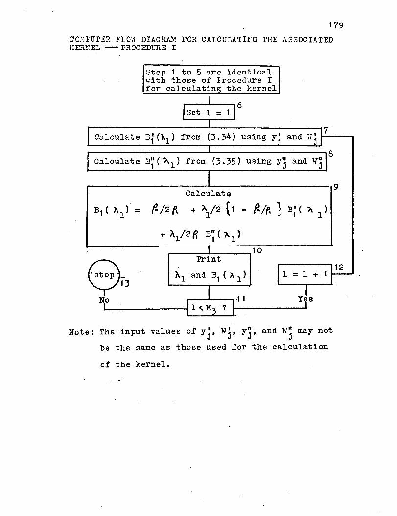
179

cm.:FUTER FLOU DIAGRA!-! FOR CALCULATI:t-JG THE ASSOCIATED KERNEL -PROCEDURE I

Step 1 to 5 are identical 1-;i th those of rrocedure I for calculating the kernel

I 1 i 6 rset 1 =

I B1(~1) (3.34) using

17. Calculate from y' and 1"1' :1 j I

I 8

Calculate B" ( ~ ) 1 1 from (3.35) using y• and \'I" j j

I Calculate

B1 ( i\1) = f../2 r. + A1/2 f 1 - f,.jp.} B;( i\ 1)

+ ~1/2 f. B" ( ). ) 1 1

I 10 Print

). 1 ·and B1

( A 1 ) 1 = 1 + 1 e-13

I -~ 1 1 ~0 .I ? I

y s 11 < M3 I

Note: The input values of y j, W j, Yj, and l'lj may not

be the same as those used for the calculation

of the kernel.

9

12

180

CONFUTER FLOU DIAGRAN FOR CALCULATING THE ASSOCIATED · KERNEL- PHOCEDURE II

Steps 1 to 5 are identical uith those of Proeedure II for calculatin~ the kernel

fset 1 = 1 J 6

7 Calculate B; ( ">. 1) from (3. 34) using y·j and Hj 1

I 8 Calculate B;' ( ">t 1) from (3.38) using y" and W"

j j

9 Calculate

Bl ( ~1) - f../2 p. + \/2 t 1 - f.../f. 1 B{ ( "1)

+ "1/2 B" ( ~ ) 1 1 I

t

13 10 1~ - I 1 Stop - 1 + Print -.

Al and Bl ( ).1)

:N 0 ' YE's

1 1 - 1 < l-!3 ?

-

APPENDIX F

EXAMPLES OF THE ANALYSIS OF THE FOUR-LAYER KERNEL

AND ASSOCIATED KERNEL

181

0.8

0.7

o.6

0.5

o.4.

0.3

0.2

0.1

182

f. : ~ : fa : ({ = 1 : 1/3:3: 1 /1 0

• d 1 :d2 :d3 = CD 1:4:1

® 1 :3:2

G) 1:2:3

@ 1 :1 :4

1.2 . 1.4 ">..---~

Fig. F.1. Examples of the curves of kernel of fourlayer earth.

183

1000 800

6oo soo

4oo

300 f ,

200 logJT2 1 vs. ~ f ~'I .

'/ Asymptote of

100 ~-log tT21

80 I 60 I 50 I 40 I 30 I 20 I

I I log 1·~ I vs. ~

I " I Asymptote of

I log rT11

I I

I,. ./_/

2 ~;/

--..._logf~l vs.~ I I

1~--~--~--~--~--~--~----~--~--~~ o.2 o.4 o.a 1.0 1.2 o·

Fig.

~ » F.2. Analysis of a four-layer kernel by numerical graphical method. Case f.: {{ : ~: f~ :1:1/3:3:1/10, d 1 : d2: d3 = 1 :4: 1 •

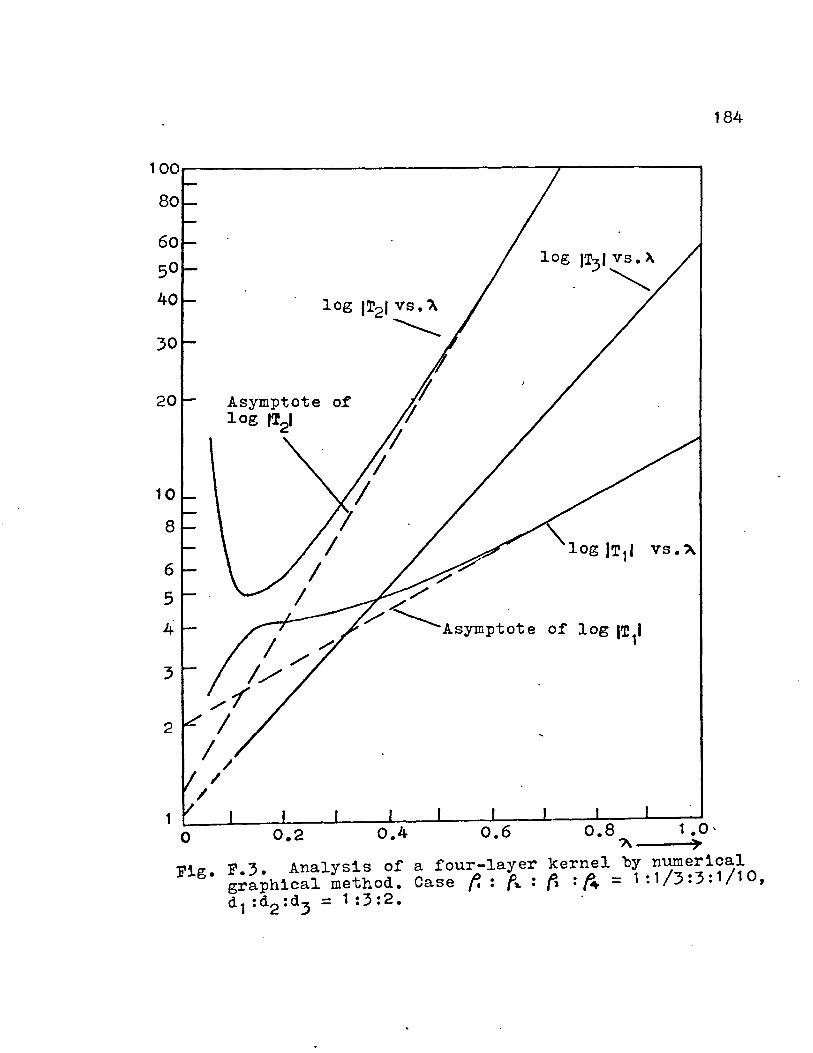
184

100r-------------------------------~-----------

6

5

4

3

2

1 0

Asymptote of log fT21

1/ //

,1 I

1/ /

/

0.2

of log IT 1 1

0.6 0.8 1~0· 7\ ~

Fig. F.3. Analysis of a four-layer kernel by numerical graphical method. Case f.: f .. : f, :f.., = 1:1/3:3:1/10, dl :d2 :d3 = 1 :3:2.

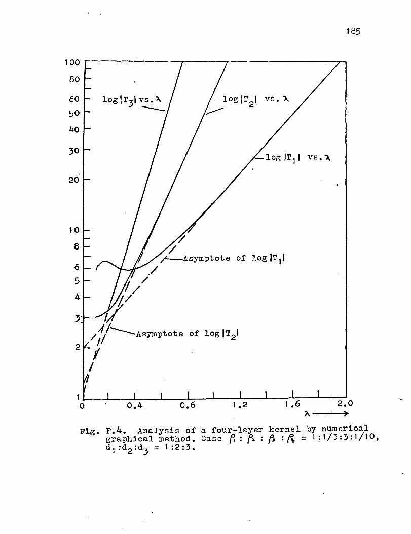
185

100 r---------------,-----~------------------~

80

60

50

40

30

20

10

8

6

5

4

2

vs. 'X

vs. 'X

0.4 0.6 1 • 2 1 .6 2.0 A---~>

Fig. F.4. Analysis of a four-layer kernel by numerical graphical method. Case f.: fa : ~ :f., = 1:1/3:3:1/10, d 1 : d2 : d3 = 1 : 2 :3 •

.,.

8

6

5

4

3

2

0.4 0.8

vs. ")\

logfT 1 vs.~ 2

Asymptote of log IT 11

1.2

186

2.0

Fig. F.5. Analysis of a four-layer kernel by numerical -graphical method. Case {'. : fi. : f:~. : f, = 1:1/3:3:1/10, d,:d2:d3 = 1:1:4,.

187 f 6.5

B,C >.)

3.5

2.5

2.0

f. : fa : !i ({ = 1 : 1 /3 : 3 : 1 I 1 o

d1 :d2 :d3 - <D 1 :4:1

@ 1 :3:2

G) 1 :2:3

® 1 : 1 :4

Fig. F.6 •. Examples of the curves of associated kernel of four-layer earth.

188

1000 ~------------,-----------------------~-------800

600 500 400

300

2oo

tOO

80

60 50 40

30

20

10

8

6 5 4

3

2

of

I I I I I / I /

I / I / 1/ / /

•/ /

/ /

1 ~------~------~--------~------~~------~~ 2 3 4 5

X---~> 0 1

Fig. F.7. Analysis of a four-layer associated kernel by numerical-graphical method. Case f, : f .. : fs: f~= 1 : 1 /3:3: 1 11 o, d 1 : d2 : d3 = 1 :4: 1 •

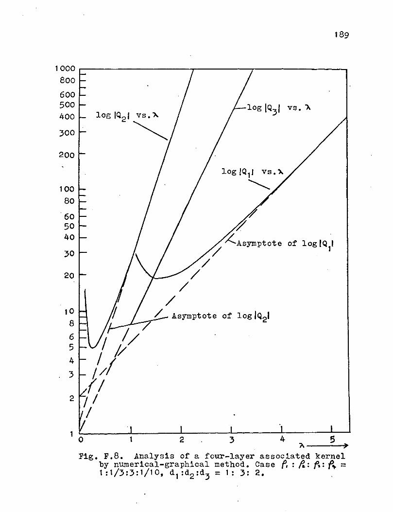
189

1000~----------------~~--------~---------------

800

600 500 400

300

200

100

80

60 50 40

30

20

10

8

6 5

4

3

2

log IQ2 1 vs. '>-.

~

1 0 1 2 3 4 5 A---~~

Fig. F.8. Analysis of a four-layer associated kernel by numerical-graphical method. Case f, : f..: fs: f..., = 1:1/3:3:1/1 o, dl :d2:d3 = 1: 3: 2. .

600 500 400

3oo

200

·1 00

80

60 50 40

30

20

10

-a 6 5 4

3

2

1 0 1 2 3 4

190

5 "---~

Fig. F.9. Analysis of a four-layer associated kernel by numerical-graphical method. Case f. : ~ : f,: f,.. = 1:1/3:3:1/10, d1 :d2:d3 = 1:2:3.

·.600 500 400

300

200

100

80

60 50 40

30

20

10

8

6 5 4

3

191

1 L-------~------~--------~------~------~~~ 0 1 2 3 4 5

~--~

Fig. F.10. Analysis of a four-layer associated kernel by numerical graphical method. Case f. : ~ : f, : f.., = 1 : 1 /3 :3 : 1 I 1 o, d 1 : d2 : d 3 = 1 : 1 :4.

VITA

Sieu Hung Chan, son of 1-iai ;·:oh Chan and Ee ~·~an Au,

was born Septecber 21, 1937, in ~ronoh, Ferak, Kalaysia.

He attended the Yoke Choy Primary School in Ipoh, Perak,

and graduated from the Chung Ling High School, Penang,

192

in Decenber 1956. In September 1957 he was enrolled into

the Can borne School of Eines, Can borne, Corm·:all, England,

from which he received the first class Associateship

of Camborne School of Mines ( A.C.S.M. ) in Kay 1960.

Ee then proceeded to 1-iissouri School of !·:ines and·

J.:etallurgy, Rolla, Hissouri, to pursue e;raduate study

in September 1960 and graduated with the degree of

!-~aster of Science in 1/.ining Engineering in Eay 1962.

After graduated from Vissouri School of Kines and

Ketallurgy he returned to Malaysia where he was employed

as a prospecting engineer by the Eastern 1-:ining and

Eetals Co:c::pany, Kuala Lu::npur, Selangor. His experience

with the Eastern ~ining and ~etals Company was primarily

concerned with the application of geophysical methods to

the search for iron ore deposits in West ~alaysia. In

the follm;ing year he became the mine manager of the

Sec;anat Iron 1-iine Ltd., in Sega!nat, Johore. In June 1 964

he joined the Derartment of Geology, University of ~alaya,

as an assistant lecturer and was pro~oted to lecturer in

January 1966. In AUGUSt 1967 the Council of University

o:f l:alaya e;ranted hin a study leave of three years, thus

enabling hi..o to return to the University of !:issolu·i at

Rolla to ~ursue his doctoral study in geophysical

engineering. He has been granted research assistantship

by the Departrr.ent of Eining and :tetroleum ::=:::nc;ineering

since September 1967. ~hile he was in the University

of l•:c:.laya he tau[;ht courses in engineering c;eology,

econo~ic geology of 5ineral deposits, and applied

geophysics, and at the same time he also carried out

research on the application of ceorhysical cethods to

the prospecting of alluvial tin deposits in West

Ealaysia.

In 1 963 he Kas JT.arried to for::er I.ee Kheng Eeh of

Singapore. They have a daughter Yik ~ei Chan who is

five years old.

193

a theoretical study on the interpretation of resistivity

Documents