a theoretical and empirical analysis of the impact of dual
TRANSCRIPT

A theoretical and empirical analysis of theimpact of dual income taxation on
economic growth
Sebastian Ellingsen
Thesis for Master of Philosophy in Economics
Department of Economics
University of Oslo
May 2014

Preface
This thesis is written as a completion of the Master of Philosophy
in Economics at the University of Oslo. Approaching the end of my
time at the University of Oslo, I would like to use this opportunity
to thank all the people of who I am indebted to for their encourage-
ment and support throughout; fellow students, family and Caroline
(who has had to endure her share of economics-talk over the years).
In particular I wish to thank my supervisor Thor Olav Thoresen, for
the time and effort he has spent providing excellent supervision and
inspiration through the work with the thesis. His guidance in navigat-
ing the literature on which this thesis is based has been invaluable. I
would also like to thank Victoria Sparrman for providing me with part
of the data set used in this thesis and Alessia Russo for helping me out
with insights on economic modeling. In addition I would also like to
thank Oslo Fiscal Studies for granting me their scholarship, for which
I am very grateful. Any remaining mistakes or inaccuracies are mine,
and mine alone.
i

Summary
Tax systems distort economic behavior in ways that matter for eco-
nomic growth. It has been argued that a dual income tax reform can
alleviate some of these distortions. The dual income tax potentially
has influence on output growth through increased allocative efficiency
of capital and increased saving and investment. The long run im-
pact of a dual income tax reform is studied in a neoclassical growth
model with endogenous labor supply. In this framework, changes in
tax rates in line with dual income taxation causes growth in excess of
the equilibrium growth rate. The effect of dual income tax systems
on economic growth is analyzed empirically by estimating a reduced
form macroeconometric relation using aggregate data for a number of
OECD-countries. The results are consistent with previous studies in
the field. The findings suggest that the dual income tax has had a
small positive effect on economic growth. When correcting for data
on corporate income taxes this effect is reduced, suggesting a substan-
tial amount of the effect of dual income income taxation on growth is
driven by reductions in corporate income taxes.
ii

Contents
1 Introduction 1
2 Theoretical analysis 4
2.1 Theories of economic growth . . . . . . . . . . . . . . . . . . 5
2.2 The model . . . . . . . . . . . . . . . . . . . . . . . . . . . . . 8
2.2.1 Households . . . . . . . . . . . . . . . . . . . . . . . . 9
2.2.2 Firms . . . . . . . . . . . . . . . . . . . . . . . . . . . 14
2.2.3 Equilibrium . . . . . . . . . . . . . . . . . . . . . . . . 15
2.2.4 The government . . . . . . . . . . . . . . . . . . . . . 16
2.2.5 Steady state . . . . . . . . . . . . . . . . . . . . . . . . 17
2.3 Taxation of capital income . . . . . . . . . . . . . . . . . . . . 20
2.4 Double taxation of capital . . . . . . . . . . . . . . . . . . . . 22
2.5 Taxation of labor income . . . . . . . . . . . . . . . . . . . . 24
2.6 Taxation of consumption . . . . . . . . . . . . . . . . . . . . . 25
2.7 The dual income tax in the neoclassical growth model . . . . 28
2.7.1 Extensions . . . . . . . . . . . . . . . . . . . . . . . . 29
3 Empirical analysis 30
3.1 Empirical background . . . . . . . . . . . . . . . . . . . . . . 30
3.2 Data description . . . . . . . . . . . . . . . . . . . . . . . . . 31
3.3 Econometric specification . . . . . . . . . . . . . . . . . . . . 35
3.4 Results . . . . . . . . . . . . . . . . . . . . . . . . . . . . . . . 37
3.4.1 Econometric challenges . . . . . . . . . . . . . . . . . 40
3.4.2 Additional explanations . . . . . . . . . . . . . . . . . 43
3.4.3 Extensions . . . . . . . . . . . . . . . . . . . . . . . . 45
4 Conclusion 45
iii

A
Theoretical appendix 53
A.1 A solution to the household’s problem with taxation of capital
and labor income . . . . . . . . . . . . . . . . . . . . . . . . . 53
A.2 Growth in labor supply . . . . . . . . . . . . . . . . . . . . . 54
A.3 A solution to the firm’s problem . . . . . . . . . . . . . . . . 55
A.4 The growth rate of capital per efficient capita . . . . . . . . . 55
A.5 The firm’s problem with non-neutral taxation of profits . . . 56
A.6 Growth rates in consumption and capital . . . . . . . . . . . 58
A.7 Steady state . . . . . . . . . . . . . . . . . . . . . . . . . . . . 58
A.8 Production efficiency . . . . . . . . . . . . . . . . . . . . . . . 59
B
Empirical appendix 61
B.1 Testing for robustness of the results . . . . . . . . . . . . . . 61
B.2 Testing for unit roots in a panel data setting . . . . . . . . . 61
iv

1 Introduction
Raising revenue from taxes distorts economic behavior by changing the rel-
ative prices of various forms of market activities. In general, this has an
impact on how resources are allocated by the market. On the other hand,
generating enough revenue is necessary for a government to finance many of
the preconditions of a functioning market economy. Thus, raising a given
amount of revenue in the least distortionary manner is the main tension in
designing tax systems. The extent to which this endeavour is successful, has
potentially large implications for welfare, see for example the recent Mirlees
review, (Mirlees et al. (2011)). The nordic system of dual income taxation
(henceforth DIT) is a particular approach of dealing with this issue. It is
a tax system that divides the total income in earned income and capital
income, taxing these sources of income at different schedules. It implements
a low and flat tax schedule on capital income in combination with progres-
sive taxation of labor income. The DIT can be interpreted as a compromise
between incorporating theoretical insights from optimal tax design, calling
for zero taxation of capital, as analyzed by Judd(1988) and Chamley(1986),
and practical concerns such as raising enough revenue and distributional
concerns, as highlighted for instance by the OECD (2006) and Piketty and
Saez (2012). A key argument for the DIT is it’s alleged positive effect on
economic growth through increased allocative efficiency capital. However,
even though there have been evaluations of the effects of the DIT; examples
in the nordic countries are Thoresen and Alstadsæter (2008), Lambert and
Thoresen (2009) and Thoresen et al. (2012), there have been no studies to
my knowledge investigating the influence of DIT on economic growth em-
pirically. Addressing this issue constitutes the aim of this master thesis.
A DIT system comprises of several features according to Sørensen (2005)a.
It has a flat uniform tax rate on all forms of capital income, equal to the
1

corporate income tax. There is full relief of double taxation of corporate
income.1 The tax base on capital and corporate income is broad. It also
has a basic tax rate on personal income, equal to the corporate tax rate,
combined with a progressive surtax. In sum, the essence of the DIT is to
tax all types of capital at the same low and flat rate, while keeping the labor
income tax schedule progressive. There is a growing theoretical literature
on the properties of such a tax system, see Boadway (2005), Sørensen and
Nielsen (1997) and Sørensen (1998), highlighting both economic efficiency
and equity considerations. Less has been written about the relation to eco-
nomic growth. However, Keuschnigg and Dietz (2007) and Radulescu and
Stimmelmayr (2005) suggest DIT reforms for Switzerland and Germany re-
spectively, and argue that an implementation of a pure form DIT system
would have a positive impact on economic growth in these countries. In sec-
tion 2 I discuss the effects that are likely to be the most important factors in
explaining the impact of the DIT theoretically in neoclassical growth model.
The aim is to make qualitative predictions. Depending on initial conditions,
the model predicts the DIT to increase capital intensity. The impact on
labor supply is vulnerable to changes in the exogenous parameter values.
Several countries, in particular the nordic countries, modernized their
income tax systems in line with the DIT in the early 1990’s. They went
from comprehensive income tax systems that were regarded as highly dis-
tortionary, to implementing features with key characteristics of the DIT.
These tax reforms had many common elements. They lowered the tax rates
on personal capital income and corporate income. In addition, these re-
forms all went far in attempting to remove double taxation of equity and
1The manner in which this is done may vary. In Norway after 1992 this was done by
the so called imputation system. There was full deduction of the tax allready paid at the
corporate level. Since the rates on personal capital income and corporate income were the
same this amounted to the same rate on dividends as on other personal capital income.
2

taxing different types of capital at the same rates. In recent years, many
other countries have made moves towards DIT systems, (Eggert and Genser,
(2005)). Several countries have introduced low flat rates on some types of
capital income, resulting in tax systems that may be termed semi-dual in-
come tax systems, (OECD, (2006)). The fact that different countries have
implemented different aspects of the DIT highlights that the distinction be-
tween comprehensive and DIT systems are not easily determined.
There is a large empirical literature on the relationship between tax
design and economic growth, with contributions applying both aggregated
and disaggregated data, see Myles (2009)a. The literature using aggregate
data is part of a larger literature conducting cross-country comparisons to
estimate the importance of various determinants of economic growth, see for
example Barro (1996) and Mankiw, Romer and Weil (1992). Recent contri-
butions relating economic growth to tax design are Lee and Gordon (2005),
Arnold et al. (2011), OECD(2010), Acosta-Ormaechea et al. (2012) and
Arnold (2008). These studies use cross-country panel regressions to analyze
the relationship between various taxes and economic growth. They estimate
the impact of different tax variables controlling for various determinants of
growth that have been established by previous studies. In this master thesis
I will to a large extent follow this approach, using macroeconomic data in a
panel data setting. However, my approach differs in taking explicit account
of the DIT systems.
This master thesis is organized as follows. In section 2 I use a growth
model to illustrate and discuss several of the properties DIT systems poten-
tially have on economic growth. The model is an infinite horizon neoclassical
growth model with endogenous labor supply. In section 2 I derive the model
and look at the effects different taxes have on the long run equilibrium. The
3

model shows that taxing capital income and firm profits reduce the long
run steady state capital stock, thus reducing growth. In this framework,
taxing capital and corporate income in line with the DIT will cause positive
growth rates. Changes in labor supply will also occur, however, this effect
depends on the numerical values of the parameters chosen in the model and
the initial state of the economy, thus the prediction on labor supply is less
clear. In section 3 I test the predictions of the model empirically using a
panel of aggregate data from a subsample of OECD countries. Controlling
for variables often cited to explain growth performance, I use the countries
that according to the OECD (2006) implemented dual income taxes in the
early 1990’s to investigate wether correlations in the data are in line with
the predictions of the theoretical model of section two. Using well estab-
lished methods in the literature on empirical growth I find some suggestive
evidence for the predictions of the theoretical model. The data shows a
positive and significant impact of the DIT systems that were implemented
in the Nordic countries in the early 1990’s on growth in GDP per capita.
Section 4 concludes.
2 Theoretical analysis
The theoretical literature on economic growth is large. When studying dif-
ferent determinants of economic growth, it is well established that the cau-
sation runs in several directions. My aim is to study the causation from
taxation to economic growth. Myles (2009)b illustrates this particular in-
teraction in the following manner,
g = f(a1(t), ..., an(t)). (1)
The growth rate g of the economy is a function of all the determinants of
growth, the vector a. Some of these determinants cause only transitory
4
changes in growth rates, typically changes in the accumulation of different
productive assets. Others however, cause changes in long-run productivity
growth. All these determinants in a are in turn a function of the tax sys-
tem, the vector of all feasible tax instruments t. The functional form of f
potentially varies among different economies and over time.2 Thus, in order
to assess the effects of a particular tax system on economic growth, the most
important determinants must be identified along with the most important
effects the various tax changes have on these.
Theories of economic growth offer a range of explanations on the de-
terminants of economic growth and their relative importance. While there
is more controversy in the determinants of an economy’s equilibrium growth
path, there is a wide acceptance in economics that accumulation of produc-
tive assets has a positive impact, at least on transitory growth rates. This
will remain the main focus of my analysis, however, other theories of growth
are also important when finding control variables for the empirical speci-
fication. I therefore survey the main insights of economic growth theory
below.
2.1 Theories of economic growth
The main insight in early growth theory is that the ultimate determinant of
economic growth is increased productivity. Accumulation of resources must
reach a steady state intensity due to depreciation and the law of diminish-
ing returns.3 Changes in investment and saving behavior may thus influ-
2This issue makes pooling of the data an overly restricitve assumption. Including a
fixed effects formulation may to some extent alleviate this, as is done in the empirical
section.3This is the main contribution of the Solow model, (Solow (1956)). A constant saving
rate will increase output per capita as long as the contribution of the saved capital exceeds
the constant share of depreciation. As the output grows, diminishing returns kicks in and
5

ence transitory growth rates of the economy, Solow (1956). This approach
was later combined with theories on how optimizing consumers adjust their
investment behavior intertemporally, as modeled in Ramsey (1928). Neo-
classical growth theory is the study of how an economy grows when it is
organized in competitive markets. The level of output is then determined by
individual’s incentives to accumulate productive assets. With this frame of
reference, taxation can be interpreted as distorting relative prices and there-
fore changing the market equilibrium. Thus, taxation might cause changes
in an economy’s long-run equilibrium output caused by changes in capital
intensity and labor supply. Immediate examples are saving and investment
decisions and therefore accumulation of physical and human capital. Taxa-
tion not only affects the stock of productive assets in steady state, but also
the composition of these. It is therefore a possibility that taxation leads to
lower productivity due to an inefficient composition of inputs in production.
For example, perfectly competitive markets would align the after tax rate of
return to physical and human capital. If one of the factors is taxed dispro-
portionally, the market aligns the after tax returns, possibly giving another
human capital and physical capital ratio in equilibrium. This will decrease
the level of production possible at a given endowment of resources.
These models all assume an exogenous growth in productivity. As in
the simple Solow model, the law of diminishing returns eventually kicks in,
(Solow (1956)). There are a number of models that have endogenised pro-
ductivity growth. Some models explain long run growth as a consequence of
positive externalities in the growth process, see for example Romer (1986).
Other theories attempt to explain the determinants of the growth rate in
productivity as a consequence of individuals and firms incentives. Firms,
a steady state intensity of capital per capita is reached in which the depreciation in each
period equals the contribution of capital on increased output. This intuition is also key
in the model applied in the next section.
6

entrepreneurs and individuals have incentives to invest in sectors of the
economy that have important productivity spill-overs into the overall econ-
omy. The general idea is that private agents do this because it lets them
extract rents from these activities and innovations, (Acemoglu (2009)). In
addition, competition among firms is viewed as a driver of the incentives
to innovate. These ideas stem from the Schumpeterian growth literature,
surveyed in Aghion and Howitt (1998). There is an influential literature
simulating tax reforms using endogenous growth models, see for example
Barro (1990). This literature concludes that tax reforms can have perma-
nent effects on the growth rate of an economy. However, these models are
highly sensitive to changes in parameter values, a problem when considering
the uncertainty in the estimation of these, (Engen and Skinner (1996)).
A different approach is to address the influence of growth on policy,
i.e turn the relationship around. The political economy of economic growth
addresses these issues, ways in which a society aggregates individual pref-
erences into policy. Some institutional arreangements thus lead to policies
that favor economic growth. Alesina and Tabellini (1990) and Persson and
Svensson (1989) are examples of this approach. In this view, the deter-
minants of economic growth are the characteristics of societies that choose
policies that favor growth.4 Making policies and institutions endogenous
poses problems for the empirical study of taxation and growth, there are
few remaining exogenous factors that can be applied for empirical analysis,
(Easterly and Rebelo (1993)).
All these issues have implications for the interpretation and formula-
tion of the empirical model. However, including these issues in a theoretical
4I think this is an important aspect of the DIT. There might be gains from commitment
when the principle of equal taxation of various sources of capital is adhered to.
7

model quickly makes it vulnerable to changes in the parameters. The theo-
retical approach chosen here is the neoclassical growth model. This model
highlights issues I believe, based on the Nordic experiences, are most preva-
lent when it comes to a shift towards the DIT and those that are able to
explain effects that can be carried over to an empirical investigation.
2.2 The model
In this section I use a growth model to illustrate the long-run effect on
equilibrium capital intensity and labor supply of introducing various taxes.
The aim is to set up a general framework to study the impact of taxes
on economic growth and use this to analyze how changes in tax rates in
line with dual income tax reform changes the market equilibrium and long-
run steady state of the model. The model is a neoclassical growth model
with endogenous labor supply. It is a model of a homogenous population
with inhabitants, organized in households, that consume and supply labor
in perfectly competitive markets. Having a homogenous population is a sim-
plifying assumption that is chosen because the aim is to conduct a positive
analysis of the qualitative implications of the DIT on economic growth. The
consumers’ incentive to smooth consumption over time, gives them an in-
centive to save by investing part of their wage in the production process of
the economy, thereby increasing output. In this model the focus is on tax
distortions. Therefore, what the government does with it’s revenue is held
exogenous. This type of model is widely used in the literature on economic
growth. The standard neoclassical growth model of the type used here is
presented in Barro and Sala-i-Martin (2004), Acemoglu (2009) and Romer
(2012) in great detail. However, I expand the model with government con-
sumption and different types of taxes in order to use it to study the impact
of DIT on economic growth.
8

2.2.1 Households
The economy is inhabited by households that receive utility over consump-
tion today and over an infinite horizon. There is an exogenous rate x,
of labor augmenting productivity growth. Productivity at time t is thus
A(t) = A0ext. The household also discounts the future at a rate 0 < ρ < 1
and therefore cares less about future consumption. In this theory of con-
sumer behavior, a concave utility function creates an intertemporal trade-off
that induces households to save, forego consumption today to consume it
in the future. At the same time, the household chooses its labor supply
at each period t. This is modeled as a trade-off between consumption and
leisure. Only by foregoing leisure is it possible for the consumer to produce
in a labor market at a given wage.
The behavioral assumption on the household is that it chooses consump-
tion and labor supply at each time t to maximize its utility. U is regarded as
a continuous and discounted sum of utility that is increased by consumption
c, and reduced by work effort, l. The utility of the consumer at t = 0 is
given below.5
U =
∫ ∞0
u(c, l)e−ρtdt (2)
A widely used functional form in macroeconomics and growth literature
is the log utility function which is separable in labor. In line with Barro and
Sala-i-Martin (2004) I assume the following functional form of the instanta-
neous utility function,6
5It follows from this framework that the household’s problem is the same for all times
t.6This function is the asymptotic case of a more general class of utility function, the
constant elasticity of substitution utility function. A maximum of the consumers prob-
lem is achieved if the following assumptions on the instantaneous utility functions are
introduced, u′(c) > 0, u′′(c) < 0, u′(l) < 0, u′′(l) > 0.
9
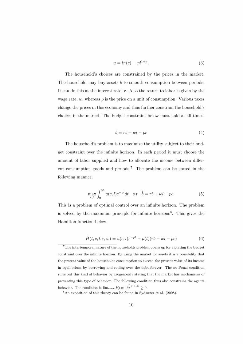
u = ln(c) − ϕl1+σ. (3)
The household’s choices are constrained by the prices in the market.
The household may buy assets b to smooth consumption between periods.
It can do this at the interest rate, r. Also the return to labor is given by the
wage rate, w, whereas p is the price on a unit of consumption. Various taxes
change the prices in this economy and thus further constrain the household’s
choices in the market. The budget constraint below must hold at all times.
b = rb+ wl − pc (4)
The household’s problem is to maximize the utility subject to their bud-
get constraint over the infinite horizon. In each period it must choose the
amount of labor supplied and how to allocate the income between differ-
ent consumption goods and periods.7 The problem can be stated in the
following manner,
maxc,l
∫ ∞0
u(c, l)e−ρtdt s.t b = rb+ wl − pc. (5)
This is a problem of optimal control over an infinite horizon. The problem
is solved by the maximum principle for infinite horizons8. This gives the
Hamilton function below.
H(t, c, l, r, w) = u(c, l)e−ρt + µ(t)(rb+ wl − pc) (6)
7The intertemporal nature of the households problem opens up for violating the budget
constraint over the infinite horizon. By using the market for assets it is a possibility that
the present value of the households consumption to exceed the present value of its income
in equilibrium by borrowing and rolling over the debt forever. The no-Ponzi condition
rules out this kind of behavior by exogenously stating that the market has mechanisms of
preventing this type of behavior. The following condition thus also constrains the agents
behavior. The condition is limt→∞ b(t)e−∫ t
0r(s)ds ≥ 0.
8An exposition of this theory can be found in Sydsæter et al. (2008).
10

The problem has the following first order conditions.
(i) u′(c)e−ρt − µ(t)p(t) = 0
(ii) u′(l)e−ρt + µ(t)w(t) = 0
(iii) µ′(t) = −µ(t)r
Using (i) and (ii) the condition for optimal labor supply of the household
directly.
−u′(l)
u′(c)=w
p. (7)
In each period the household will supply labor in the market up to an amount
such that the marginal disutility of working is exactly offset by the marginal
return measured in utility of supplying another hour in the labor market. In
this situation there are no further gains from trade between the household
and the firm in the labor market.
Taking the derivative with respect to time of (i) and combining it with
(iii) gives the optimal path of consumption. The first order conditions of
the problem will result in the following differential equation that describes
the optimal path.
r = ρ− cu′′(c)
u′(c)
c
c− ∂u2
∂c∂l
l
u′(c)
l
l+
p
1 + p. (8)
The second expression on the right hand side equals the elasticity of marginal
utility with respect to consumption.
ε = −u′′(c)
u′(c)c. (9)
11

This gives the following optimal path9,
r = ρ+ εc
c− ∂u2
∂c∂l
l
u′(c)
l
l+
p
1 + p. (10)
The condition states that along the optimal path the marginal gain in post-
poning a unit of consumption equals the marginal discounted realized return
in the market. ε is the elasticity of marginal utility and therefore measures
the concavity of the utility function.10 The concavity measures the strength
of the households’ incentive to smooth consumption in the market. There-
fore the more concave the utility function is, the smaller is his incentive
to adjust to changes in the rate of return, thus the smaller the change in
consumption growth. If the marginal utility of consumption is linear, the in-
centive to smooth consumption is weak, resulting in a household that reacts
extensively to changes in the market return. In the presence of a positive
exogenous growth rate in prices, the real return of foregoing consumption
today is reduced. In isolation this will discourage saving and investment of
the household in the same way as a reduced interest rate.
The cross derivative of labor and consumption measures the extent to
which consumption and leisure are complements or substitutes.11 If the
cross derivative of consumption and work effort is negative, the household
gets less utility from a marginal increase in consumption the higher the work
effort is. In the case with growth in labor intensity the household has even
less incentive to save since future marginal utility of consumption decreases
as the work effort then will be higher. If the cross derivative is positive, the
9Mangassarian’s theorem states that satisfying the conditions for the maximum princi-
ple is sufficient for the path to be a maximum as long as the Hamilton function is concave
in the controll variables, as is the case of this problem, Sydsæter et al. (2008).10The more concave the utility function is in c the higher is ε.11Intuitively, this derivative measures the extent to which the household enjoys con-
sumption in the time off work.
12

marginal utility of consumption increases with labor supply. In this case the
household has an additional incentive to forego present consumption. If it
is zero, only market return and the incentive to smooth consumption mat-
ters for the saving decision. These are interesting properties that describe
how investment and saving decisions might be influenced by decisions in the
labor market. If the instantaneous utility function takes the form above
consumption and leisure are two isolated sources of utility and the cross-
derivative equals zero. The differential equation for consumption growth is
then given by the expression below.
c
c=r − ρ
ε, (11)
In the model there is an exogenous labor augmenting growth rate in
productivity and an endogenous growth in labor supply. To study the long
run equilibrium in such a model it is usual to rewrite the stocks in per
efficient capita terms.12 The growth rate in consumption per efficiency unit
of labor is therefore given by the following equation,
˙c
c=r − ρ
ε−[x+
l
l
](12)
With the functional form above the condition for optimal labor supply is
given by the expression below.
ϕ(1 + σ)clσ =w
p(13)
This expression can be written in per capita form in the same manner, this
is shown in the appendix and yields the following expression,
ϕ(1 + σ)lσ+1 =(1 − α)kα
c(14)
12As is usual in models of growth the variables denoted with a hat are measured in per
efficient unit of labor.
13

This expression is needed to find the labor supply in long run equilibrium.
Labor supply is determined endogenously in the model. This means that
knowing the real wage and consumption, the labor supply of the maximizing
household must follow. Knowing the growth in consumption and the real
wage it is possible to deduce the growth rate in labor supply in the model,
this is shown in the appendix. With the functional form chosen there is zero
growth in labor supply in long-run equilibrium. The growth in the real wage
is exactly offset by the growth in consumption.
2.2.2 Firms
It is necessary to know how production takes place in order to study the
market equilibrium of the economy. The model consists of many firms pro-
ducing the consumption good, acting in a perfectly competetive manner.
The firms can therefore be aggregated in a production function which will
be analyzed in the model. The firms choose between the different input
factors and level of production given market prices in order to maximize
the profits. As with the consumers, the firms have to take the market en-
vironment as given and then decide how to behave optimally constrained
by market prices and technology. The representative firm’s problem can be
stated in the following manner,
maxI,L
π =
∫ ∞0
[pf(K,L)−qI−wL]e−rtdt s.t K = I−δK, K(0) = K0 (15)
The firm maximizes the present value of profits over an infinite horizon
by choosing inputs optimally to given prices. I solve the problem using
optimal control theory as shown in the appendix. The solution to the profit
maximization problem is given by the usual first order conditions. The value
of the marginal product equals the factor price for all t. The cost of investing
for the firm is denoted by q. In the following I will assume that investment
14

is costless for the firm.13
w(t) = pf ′(L), r(t) = pf ′(K) − δ. (16)
The aggregate production function takes the Cobb-Douglas form, shown
below,
y = Kα(AL)1−α. (17)
In per efficient capita terms the production function is given by the following
expression,
y = kα. (18)
This gives the following expressions for the market return to labor and cap-
ital,
w(t) = pA(t)(1 − α)kα, r(t) = pαkα−1. (19)
From this we see that the real return to labor and capital is increasing due
to the exogenous technical rate of change that is present in the model. At
all times the rate of return to different factors of production is governed by
the marginal product. This is a consequence of perfect competition; there
can never be any remaining gains from trade in equilibrium. This will be
elaborated upon in the next subsection.
2.2.3 Equilibrium
There are three markets in the model, a market for the consumption good,
a labor market and a market for capital.14 All these markets are assumed to
13In the sense that q=1. q > 1 could denote the reduced form of some tax distortion
that increases the cost of capital for the firm.14Actually there is a continum of markets in the model, but three markets for each time
t.
15

clear at all times t. Thus, in equilibrium the wage makes the labor supply of
households equal the labor demand of firms, ls(w) = ld(w). The interest rate
r in equilibrium makes the supply of capital of households equal the demand
of firms, K(r) = b(r). The price of the consumption good is the numeraire,15
thus all other prices are measured in terms of units of the consumption
good. Put differently, an equilibrium in this model is thus a feasible time
path of allocations [k(t), b(t), l(t), c] and prices [p, r(t), w(t), τ ], such that
the firms maximize their profits, consumers maximize their utility, resource
constraints hold and that the governments budget constraint holds. τ is a
vector of the governments tax instruments. Having defined the equilibrium
of the model there now are sufficient conditions to determine the value on
all the endogenous variables. This insight can be used to study the long run
evolution of these static equilibria to changes in tax policy as will be done
in the next sections.
2.2.4 The government
The government is modeled in the simplest possible manner. It finances its
activities by taxing different forms of income. The only fiscal instruments
the government has at its disposal are distortionary taxes. Government
spending is held exogenous in the model. The budget constraint must hold
for all times t, I ignore the governments ability to trade in capital markets.
The budget constraint is given below, where τb is a tax levied on the return
of the households investment and τw is a labor income tax.
G(t) = τbr + τwlw + τcpc+ τfπ′. (20)
In addition there is a tax rate on private consumption denoted τc. This
tax will play the role of a uniform tax on all different consumption goods.
15p(t) = 1 for all t.
16

τf is a tax on the firms profits,16 levied on a share of the firms profits to
make it non-neutral in the model. In the following I will find the reduced
form equations of the model without any taxation of distortionary taxes to
act as a benchmark case for comparison.
2.2.5 Steady state
In each period capital is invested by the household. Capital evolves in
accordance with the law of motion for capital.
K = I − δK (21)
Investment in this economy is given by the following equation,
I = rK + wl − c. (22)
Thus the growth in the capital stock is the difference of the invested capital
and the depreciation. Using the equilibrium conditions and various resource
constraints I find expressions for the growth rates of the endogenous variables
of interest.17 These expressions are given below.
˙c
c= (αkα−1 − δ) −
[ρ+ x+
l
l
](23)
˙k
k= kα−1 −
[δ + x+
l
l
]− c
k(24)
l
l=
α
1 + σ
˙k
k− 1
1 + σ
˙c
c(25)
16This is formulated as a tax on corporate profits. However, the C-D production function
has constant returns to scale, thus the only possible equilibrium profit is zero. This
problem is alleviated by the fact that I assume the government lacks perfect information
on the firms profit and therefore calculates the tax using a different tax base than true
profits.17I show this in the appendix.
17

ϕ(1 + σ)lσ+1 =(1 − α)kα
c(26)
The growth rate in consumption per efficient capita is determined by the real
return to capital because of the households incentive to save. This incentive
is reduced by the strength at which the agent discounts the future. The
exogenous growth in productivity and increases in labor supply are factors
that dilute the per efficient capita expressions. The net increase in capital
per efficient capita equals the total production minus the part consumed by
the household and the government.18 The same factors dilute capital per
efficient capita. The labor supply is determined by the ratio of consumption
and the real wage. Growth in labor supply is thus governed by the growth
in these factors.
Usually in growth models equations such as these define a system with
a saddle point equilibrium. Many of the paths rely on initial conditions
that do not make economic sense. The system can be reduced further to
find the constraints on the parameters that would ensure existence of this
equilibrium.19 Since I am not going to introduce parameter values, I just as-
sume they have appropriate values for the system to have a unique solution
and then find the closed form solution directly. Combining the equations
determines the steady state values of capital and consumption per efficient
capita, in addition to the labor supply in steady state. The steady state
variables of the system are shown below.20
18In this benchmark case G(t) = 0 for all times t.19The necessary constraints on the parameters are that the eigenvalues of the linearized
reduced form matrix needs to be less than one in absolute value and have opposite signs,
Sydsæter et al. (2008).20ss denotes the variable value in steady state.
18
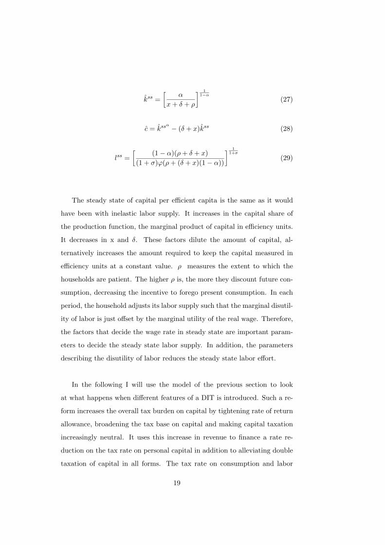
kss =
[α
x+ δ + ρ
] 11−α
(27)
c = kssα − (δ + x)kss (28)
lss =
[(1 − α)(ρ+ δ + x)
(1 + σ)ϕ(ρ+ (δ + x)(1 − α))
] 11+σ
(29)
The steady state of capital per efficient capita is the same as it would
have been with inelastic labor supply. It increases in the capital share of
the production function, the marginal product of capital in efficiency units.
It decreases in x and δ. These factors dilute the amount of capital, al-
ternatively increases the amount required to keep the capital measured in
efficiency units at a constant value. ρ measures the extent to which the
households are patient. The higher ρ is, the more they discount future con-
sumption, decreasing the incentive to forego present consumption. In each
period, the household adjusts its labor supply such that the marginal disutil-
ity of labor is just offset by the marginal utility of the real wage. Therefore,
the factors that decide the wage rate in steady state are important param-
eters to decide the steady state labor supply. In addition, the parameters
describing the disutility of labor reduces the steady state labor effort.
In the following I will use the model of the previous section to look
at what happens when different features of a DIT is introduced. Such a re-
form increases the overall tax burden on capital by tightening rate of return
allowance, broadening the tax base on capital and making capital taxation
increasingly neutral. It uses this increase in revenue to finance a rate re-
duction on the tax rate on personal capital in addition to alleviating double
taxation of capital in all forms. The tax rate on consumption and labor
19

might need to be changed to make the tax reform revenue neutral, there-
fore the long run effect of changing these tax rates is also of interest. The
analysis is in a sense partial, I regard different aspects of the dual income
tax in isolation. Although somewhat stylized, this makes the effect of each
particular tax rate clearer.
2.3 Taxation of capital income
In this section I consider a reduction the tax rate on personal capital in-
come. This changes the household’s and government’s budget constraint.
In this section I assume that the government finances all of its activity with
distortionary taxation of capital income. The budget constraints in this case
are shown below.
b = (1 − τb)rb+ wl − pc (30)
g = τbrK (31)
A fraction τb of the income from investing in capital is payed to the gov-
ernment at each time t. This changes the equation of the system in the
following manner.
˙c
c= (1 − τb)(αk
α−1 − δ) −[ρ+ x+
l
l
](32)
˙k
k= kα−1 −
[δ + x+
l
l
]− c
k− g
k(33)
l
l=
α
1 + σ
˙k
k− 1
1 + σ
˙c
c(34)
ϕ(1 + σ)clσ = w (35)
20

The steady state values of the system are then given by the following equa-
tions.
kss =
[(1 − τb)α
x+ ρ+ (1 − τb)δ
] 11−α
(36)
c = kssα(1 − ατ) − (δ + x)kss (37)
lss =
[(1 − α)kα
ϕ(1 + σ)c
] 11+σ
(38)
From these equations it becomes clear that the usual factors that deter-
mine the steady state capital stock are important in determining the impact
of taxing personal capital income. Capital taxation decreases the long-run
steady state capital intensity. In addition, capital income taxation affects
all the endogenous variables in steady state.
Tax rates on capital will have a direct influence on growth through dis-
torting the return to capital, and thus the incentive to save. When the
taxation of capital is increased people change their behavior in response
the increase. Lower return of capital induces an immediate increase in con-
sumption. When consumption increases, fewer resources are diverted to
maintaining the capital stock at its current value and hence more depreci-
ates than is invested. In the long run this decreases the capital stock, thus
reducing the productive capacity of the economy. By the same mechanism,
a reduction in the tax rate on capital will increase economic growth. More-
over, in the new steady state the level of consumption is also lower as can be
seen by comparing equation (36) with the corresponding equation without
taxation.
21

Since taxation of capital changes the values of both k and c it might
also change the steady state value of labor supply even though labor and
leisure is separable in the utility function. The reason is that labor supply
is determined endogenously in the model, given when the real wage and
consumption is given. If consumption changes relatively more than the real
wage the labor supply will decrease, while the labor supply will increase in
the opposite case. The qualitative effect of capital income taxation on labor
supply is ambiguous, depending on the parameterisation of the model.
2.4 Double taxation of capital
In addition to a tax on capital, all firms pay a share of their profits to
the government. If only pure rents are taxed, the maximization problem
of the firms is not affected and the tax is said to be neutral. It induces
no behavioral change in this case. In this section I consider a non-neutral
corporate income tax, similar to the cases studied by Sandmo (1974). This
distorts the choice of inputs for the firm. Tax rates on inputs will cause
substitution away from the relatively more expensive inputs. In this model
this can be incorporated by not deducting all the costs from the firms profits.
The firms problem is then given by the following problem.
maxI,L
π =
∫ ∞0
[(1− τ ′f )(f(K,L)−sI−wL)− (1−s)I]e−rtdt s.t K = I− δK (39)
The firm pays the share τf of the tax base to the government. However,
only a share s of the investment costs are deducted from the tax base. In
general this could stem from the governments inability to estimate the true
economic values internalized by the firm.21 The tax paid by the firm can
thus be influenced by choosing the level of investment and will distort the
21An example could be to tight depreciation allowances.
22

economic decision. As shown in the appendix, this increases the cost of
capital for the firm. The firms first order condition is given by the following
equations, where τf denotes the effective tax rate of capital.22
(i) pf ′(K)(1 − τf ) = δ + r
(ii) pf ′(L) = w
Taxing firm profits in this manner decreases the rate of return of investing in
the firm. The system now evolves in accordance with the following equations.
˙c
c= (1 − τb)(αk
α−1(1 − τf ) − δ) −[ρ+ x+
l
l
](40)
˙k
k= kα−1 −
[δ + x+
l
l
]− c
k− g
k(41)
ϕ(1 + σ)clσ = w (42)
Corporate taxation thus leads to double taxation of capital, further decreas-
ing the rate of return of investing in the production process for the con-
sumers. This further increases the tax wedge in the market for productive
capital. There is a wedge between the real value of investing an additional
unit of capital and the return at the corporate level. When this return is
eventually paid out to the investor, for instance as dividends, there is an
additional wedge caused by taxation on the personal level. The long-run
values of the endogenous variables in per efficient capita units is found in
the usual manner and are given by the expressions below,
kss =
[(1 − τf )(1 − τb)α
x+ ρ+ (1 − τb)δ
] 11−α
(43)
22As shown in the appendix, τf =τ ′f(1−s)
1−sτ ′f.
23

c = kssα − kss(x+ δ) − g (44)
lss =
[(1 − α)kα
ϕ(1 + σ)c
] 11+σ
(45)
Double taxation further decreases the rate of return to investments.
Again, this affects the tradeoff between consumption in the different pe-
riods. Increased present consumption causes less saving and therefore less
investment. When less capital is invested and the replacement ratio kept
constant, the capital stock in per efficiency units decreases. All deviations
from a corporate income tax on pure rents will have this effect in the long
run. The other equations show that it has the same effect on consumption
and the same ambiguous effect on labor supply.
2.5 Taxation of labor income
In this section I introduce a labor income tax. This changes the household’s
and the government’s budget constraint. I assume that the government
finances all of its activity with distortionary labor income taxation. The
budget constraints of the household and the government given by the ex-
pressions below,
b = rb+ (1 − τw)wl − pc (46)
g = τwlw. (47)
The tax rate on labor is denoted by τw. Taxation of labor income will change
the labor supply by altering the return to supplying labor in the market.
The system of equations with labor income taxation is given below,
24

˙c
c= (αkα−1 − δ) −
[ρ+ x+
l
l
](48)
˙k
k= kα−1 −
[δ + x+
l
l
]− c
k− g
k(49)
ϕ(1 + σ)clσ = (1 − τw)w (50)
Using the system I find the following steady state values,
kss =
[α
x+ δ + ρ
] 11−α
(51)
c = kssα(1 − (1 − α)τ) − (δ + x)kss (52)
lss =
[(1 − α)(ρ+ δ + x)(1 − τw)
(1 + σ)ϕ((x+ ρ+ δ)(1 − τw(1 − α) − α(x+ δ))
] 11+σ
(53)
Taxation of labor income has an ambiguous effect on labor supply in the
long run. Taxing labor directly reduces the real wage. However, increased
government consumption crowds out private consumption in the new long
run equilibrium. The first order condition of the intertemporal optimum
is not affected, thus the capital intensity is the same as before. Taxation
of labor income therefore does not affect investment behavior. This is a
consequence of strict separability of the utility function in consumption and
leisure.
2.6 Taxation of consumption
Taxation of consumption goods is also considered in the model due to it’s
potential role in making the change to the DIT system revenue neutral, as
25

in Keuschnigg and Dietz (2007). Taxing consumption goods changes the
budget constraint of the consumer and government in the following manner,
b = rb+ wl − (1 + τb)c (54)
g = τcc (55)
A well known result from optimal tax theory is that a uniform tax on all
goods consumed by the individual is equivalent to a lump sum tax. How-
ever, as usual the government can only tax transactions that occur in the
market, in this sense a uniform tax on all goods is impossible in practice.23
It will distort the tradeoff between market and non-market activities. In
this model, I abstract from household production. However, leisure can not
be taxed and a uniform tax on consumption will have an influence through
the labor supply decision. In addition, increasing the consumption tax may
cause distortions in the intertemporal decision of the household, since in the
reform period, changes in consumption taxation affect the relative prices of
consumption in the different periods. To show this I solve households max-
imization problem again and find the optimal path of consumption below.
˙c
c= (αkα−1 − δ) −
[ρ+ x+
l
l
]+
τc1 + τc
(56)
If the consumption tax evolves over time it will affect the households trade-
off by changing the relative prices of consumption in the different periods.
Growth in the consumption tax will have the same effect as a lower real
return to saving. It will induce the household to save less, by making future
consumption less attractive. Consumption will then evolve along a lower
23In addition, non-uniform optimal taxation of consumption goods would require large
administration costs, requiering updating the tax schedules with changes in preferences
and technology. This is likely to be highly unfavorable to economic growth because it
would hamper investment.
26

path, more is consumed resulting in a lower steady state with the usual
mechanism of dilution and depreciation. However, assuming no growth in
the consumption tax, the reform is simply a discontinuous jump that is not
anticipated by the household, in this case the derivative of the tax is al-
way zero and the term therefore vanishes. In this case there is no effect of
consumption tax on saving, the expression then becomes the familiar one
below.
˙c
c= (αkα−1 − δ) −
[ρ+ x+
l
l
](57)
˙k
k= kα−1 −
[δ + x+
l
l
]− c
k− g
k(58)
ϕ(1 + σ)clσ =w
1 + τc(59)
As with labor taxation, taxation of consumption goods does not alter the
tradeoff between periods, unless it varies over time. The steady state values
of the endogenous variables are now given by the following expressions,
kss =
[α
x+ ρ+ δ
] 11−α
(60)
c =kss
α − (δ + x)kss
1 + τc(61)
lss =
[α(ρ+ δ + x)
(1 + σ)ϕ(ρ+ (δ + x)(1 − α))
] 11+σ
. (62)
With this specification of the utility function there is no effect on the steady
state capital intensity or labor supply from taxing the consumption goods.
The only effect is through lower consumption and is thus equivalent to a
27

lump sum tax in the model. However, the reason follows from the fact that
the real wage is reduced by the exact same amount as the consumption in
long-run equilibrium. If the change in consumption did not reduce with this
amount, taxation of consumption would induce changes in labor supply.
2.7 The dual income tax in the neoclassical growth model
The introduction of a DIT system in this modeling framework implies low-
ering the tax rate on capital below that of labor. In addition, the corporate
income tax is lowered, set equal to the personal income tax on capital. Dou-
ble taxation is fully alleviated. The capital income tax base is broadened,
aiming at equalizing tax rates on various forms of capital income and assets.
Reduction of tax rates of capital income and corporate profits increases the
household’s incentive to save. Removing double taxation of capital further
decreases the wedge between the real and private return of capital. In line
with the above reasoning, this implies that more capital is accumulated than
is diluted by productivity growth and depreciation each period, hence driv-
ing the growth rate to a positive level in excess of the exogenous rate of
productivity growth. In addition, lower taxation of corporate profits and
equalizing tax rates on different types of capital will also have an effect on
the production efficiency of the economy.
In order to assess the quantitative implications of these effects and the
transitional dynamics of the model specific parameter values would have to
be introduced. However, the aim of this section has only been to derive
qualitative implications of changing tax rates in line with a DIT reform. In
sum, a DIT might cause growth through increasing equilibrium investment.
In the model this will cause a transitory effect on growth that is higher than
the equilibrium growth rate. I therefore expect to find a positive influence on
DIT and economic growth in the data. In the next section I will investigate
28

data from 23 OECD-countries evaluate this effect.
2.7.1 Extensions
To highlight some of the shortcuts and loose ends I will discuss some pos-
sible extensions of the model. An immediate extension of the model could
be to include heterogenous agents, as is done in Caselli and Ventura (2000).
Differences in skill would yield different returns in the labor market. This
would allow for introducing a progressive income tax schedule and studying
the effects on growth of changing this schedule in a DIT reform. In ad-
dition, a very natural extension would be to allow for a larger role of the
government. This could be done by letting government consumption enter
into the production function of firms or the utility of the households. In
this case, economic growth would also be influenced by changes in govern-
ment consumption and the revenue requirement of the government would
be needed to be taken more account of.24 Moreover, it would open up for
using the model to do welfare analysis. Another interesting extension could
also be to introduce different sectors of the economy. These could grow at
different exogenously given rates, inducing structural change. This model
could then be used to study tax policies in countries with large differences
in productivity growth in different sectors, such as the Norwegian economy.
Finally, open economy issues matter for growth, in a more rigorous model,
these issues would need to be taken into account.
24An interesting effect could be to look at the effect when government consumption is a
complement to private consumption, this could then induce changes changes in saving. A
way to motivate this could be that government spending on legal institutions is necessary
for complicated transactions such as saving to take place.
29

3 Empirical analysis
Although the model of the previous section is simple, it produces many
testable hypotheses regarding the relationship between taxation and eco-
nomic growth. In this section I attempt to test some of the implications of
the theoretical model in a panel of aggregate data for OECD-countries. I
will investigate if the features of the DIT system mentioned above are pos-
itively related to growth in real data. The approach taken is to investigate
the impact of tax reforms in the nordic countries that came close to a DIT
reforms, and compare these experiences with the rest of the sample. If the
effects modeled in the theoretical section are of any significance, the subset
of countries with DIT should have a higher growth rate than the others in
the period following the shift towards DIT. These tax reforms are shown in
table 1.
3.1 Empirical background
The empirical approach chosen follows a large strand of the established lit-
erature on taxation and economic growth. In this literature cross-country
panels of macroeconomic data are used to estimate the relationship between
tax rates and economic growth. Arnold et al. (2011) is an example of this
approach. They use aggregate data to investigate the relationship between
economic growth and various forms of taxes in a panel of OECD countries.
They find that tax design influences economic growth. More specifically
they find that taxation of immovable property is the least harmful, followed
by consumption taxes, personal income taxes and corporate income taxes.
They estimate that shifting 1% of the tax revenue towards the less harm-
ful taxes would increase growth between 0.25% to 1%. Lee and Gordon
(2005) use a fixed effects regression model to estimate the effect of different
tax rates on economic growth in a sample of 70 developed and developing
countries. They estimate a negative effect of corporate income taxes of eco-
30

nomic growth; a 10% reduction in the corporate income tax will increase
the growth rate with approximately 1%. Arnold (2008) also finds a negative
impact from the personal and corporate income taxes on economic growth
and concludes that taxes on immovable property and consumption are the
ones with the least negative impact on growth. Kneller et al. (1999) find
that some personal income taxes reduce growth, while for example taxation
of consumption does not seem to affect growth. Widmalm (2001) also es-
timates the effects of various forms of taxation on GDP in the OECD. She
finds a negative relationship between personal income taxation and economic
growth. However, capital taxation on the personal level is not explicitly ac-
counted for. She also concludes that taxation of consumption has the least
negative impact on economic growth.
The findings of this literature suggests that taxation and in particular
corporate and personal income taxation has an effect on economic growth.
However, due to the large technical difficulties in comparing tax rates on
various forms of capital in system with very different tax rules, this litera-
ture has to a large extent ignored including more detailed information on
the composition of the capital tax base. They mainly include information
on corporate income and taxes on housing. The literature represented by
these authors thus to a large extent ignores tax designs of capital income.
In this master thesis I attempt to take explicit account of this by including
information on one particular tax system, that of the DIT, into the empirical
analysis of taxation and economic growth.
3.2 Data description
The countries analyzed are a subset of the member countries of the OECD,
excluding the countries from Latin America, eastern-European countries and
Turkey. The data used in this analysis are available from the online data
31

Table 1: DIT reforms. The table is an extension of the table found in Sørensen (1994).
Country Personal Capital Corporate Integration
Finland
Before 1993 25-57 25-57 37 Double taxation
After 1993 25-57 25 25 Full relief
After 2005 25-57 28 26 Partial relief
Norway
Before 1993 26.5-50 26.5-40.5 50.8 Partial relief
After 1993 28-41.7 28 28 Full relief
After 2006 28-48 28 28 Partial relief
Sweden
Before 1993 36-72 36-72 52 Double taxation
After 1993 31-51 30 30 Full relief
bases of the OECD. The data on GDP,25 saving rate and net investment is
obtained from the online data base of the national accounts that are mea-
sured annually. The data on GDP is filtered using the Hodrick-Prescott
filter with a parameter of 80.26 I have applied the Hodrick-Prescott filter on
the GDP data to smooth away parts of the business cycle. The dependent
variable of the analysis is the annual change in the logarithm of the gross
domestic product. I apply control variables to account for business cycles
and growth enhancing features that are not tax related.
The explanatory variable of interest is a dummy variable which takes
the value 1 for time periods under a DIT in selected countries, see table 1.
Some of the nordic countries have implemented DIT, OECD (2010), OECD
(2006) and Sørensen (1994). This includes Norway from 1993 to the present,
25The GDP data are the purchasing-power adjusted values.26The Hodrick-Prescott filter is a widely used method in macroeconomics to filter out
cyclical components in time-series data. The method is a minimization problem, trading
off deviations from trend with a loss in correcting the time series.
32

Sweden from 1993 and onwards and Finland from 1993 to 2005. In these
countries the tax rates on capital were lowered, broadened and set equal
to the corporate income tax. This was combined with progressive taxa-
tion of labor income. However, a number of countries in the sample have
implemented tax systems that share some characteristics with that of DIT
countries, Genser and Reutter (2007). This highlights that the distinction
between countries having implemented the DIT and those who have is not
sharp. Therefore largely ignoring more detailed differences in these coun-
tries tax systems is a weakness of this analysis. The countries of the full
sample are Australia, Austria, Belgium, Canada, Denmark, Finland, France,
Germany, Greece, Iceland, Ireland, Italy, Japan, Luxembourg, Netherlands,
New Zealand, Norway, Portugal, Spain, Sweden, Switzerland, United King-
dom and the United States.
Several of the control variables are obtained from the statistics data
base of the OECD. The saving rate is measured as the net saving divided
by the gross domestic product of the country, net saving is measured as the
difference between disposable income and final consumption taken from the
national accounts. Net capital stock is the total capital, measured with 2005
as a base year and deducted for estimated capital depreciation. Inflation is
measured as yearly averages of the core inflation, provided by national statis-
tics agencies to the OECD. FDI is the inflow of foreign direct investment
as measured in thousands of American dollars. As a measure of human
capital I use a variable defined as the Barro-Lee skill ratio, (Rossvoll and
Sparrman, (2013)). It measures the ratio of the population over 15 with
some level of tertiary education. The data are taken from Barro and Lee
(2010).27 Labor participation is a the percentage of the total population
27The data set only includes 5 year averages. Rossvoll and Sparrman (2013) extend
this using a linear approximation. The data can be found at: http://www.barrolee.com.
They are also available in Barro and Lee (2010).
33

employed. The terms of trade measures the change in the import prices rel-
ative to export prices relative to its 2005 value.28 Long-run unemployment
is the share of the unemployed who have stayed unemployed for more than
12 months. The R&D intensity is measured by the R&D cost over value
added in the manufacturing sector, obtained from Rossvoll and Sparrman,
(2013). Data on corporate income taxes come from the World Tax Database
of the Office of Tax Policy Research.29 In addition the average tax wedge
is included in the data set. The tax wedge measures the sum of the direct
tax rate, employment tax rate and the indirect tax rate for a worker with
average income. The Summary statistics of all the included data is provided
in table 2.
Table 2: Summary statistics
Variable Obs. Mean Std.dev Min. Max.
Log GDP per capita 985 -6.88 1.88 -11.35 -1.7
Capital stock 223 75.89 21.61 27.05 117.37
Population growth 1177 0.707 0.5855 -2.74 4.48
Human capital 820 22.9 0.19 0.014 1.07
R&D 649 0.047 0.034 0.002 0.159
Inflation 978 4.47 3.98 -4.4 26.4
Saving rate 925 8.74 5.84 -14.82 29.99
FDI 505 22613 42570 -36602 321276
Terms of trade 924 98.66 14.1 60 191.6
Corporate income tax 667 0.365 0.1 0.125 0.61
Average tax wedge 299 36.4 10.4 15.86 57.1
DIT 58 0.039 0.194 0 1
28This variable is of particular importance when it comes to Norway which has experi-
enced high growth rates due to a large improvement in the terms of trade in the period it
has had a DIT.29http://www.bus.umich.edu/otpr/otpr/default.asp
34

3.3 Econometric specification
The regression model I will apply can be interpreted in line with the type of
model of the previous section. As is usually the case when regressing policies
on growth, I apply control variables that are widely believed to explain part
of the variations in growth rates. The formulation and included variables
follows follows the specifications in the influential papers on the empirics of
growth by Barro (1996) and Mankiw, Romer and Weil (1992). The equa-
tion estimated takes the following functional form, given that countries are
represented by subscript i and time by subscript t,
log yi,t = φ0 + φ1DITi,t + β′1Xi,t + β′2vi,t + γi + φ′2taxi,t + εi,t (63)
The dependent variable log yi,t is the logarithm of GDP per capita for coun-
try i at time t. β′1X contains the baseline model of economic growth, in line
with the model in the previous section. The coefficients of the explanatory
variables denote the change in ratio of the output of the economy for a unit
change in the variable. Growth in output is understood as the sum of the
growth rates in the stocks of the economy. It therefore includes the capital
stock and the growth rate of the population. Changes in the human capital
is also included. Increases in human capital cause changes in the produc-
tivity of each worker. In addition to increases in the economy’s stocks of
productive assets various other factors increase economic growth, through
for example productivity growth.30 vi,t is a vector of other control variables.
It contains inflation and unemployment to further adjust for the business
cycle, in addition to controlling for the negative effects these variables may
have on growth. Unemployment might influence growth through deprecia-
tion of human capital, and inflation through allocation inefficiencies. R&D
intensity will explain some differences in productivity growth. In addition
30x, in line with the model in section 2.
35

it contains variables meant to control for open economy issues, the inflow of
FDI and the change in the terms of trade. It also contains the average saving
rate in year t which is given by the first lag. taxi,t includes data on corpo-
rate income taxation and the average tax wedge. I include this to control
for other tax related issues and for robustness. The unemployment rate is
differenced because I find evidence non-stationarity in this time series. The
data are summarized in table 2. To control for unobserved differences among
countries I include country specific fixed effects, these effects are given in
the vector γ. This variable will capture some of the effects from omitted
variables that differ between countries. DITi,t is the dummy variable for
the subset of the sample that is a DIT regime.
In a panel of countries, that potentially vary greatly along many dimen-
sions it is necessary to take account of unobserved country heterogeneity.
Pooling the data in a cross-country comparison is a strict assumption and
in the presence of country specific effects this will cause an omitted variable
bias of the estimates. How this country heterogeneity is modeled empirically
potentially has a large influence on the outcome. In the econometric analy-
sis of panel data, panel specific effects are often dealt with in two different
ways, see Greene (2008). The country specific effects can be modeled either
as fixed or random effects. The random effects approach assumes that the
country specific effects are orthogonal with all the other regressors. This
amounts to assuming that all the country specific effects have no system-
atic influence on any of the explanatory variables included in the empirical
model. This seems to be unlikely when comparing countries using aggre-
gate data. The second approach is the fixed effects model. This approach
amounts to including a constant term for each country that is hypothesized
to absorb the country specific effect.31 It is also worth noting that estima-
31Using the Hausman test I find that there is not sufficient evidence in the data to reject
36

tion using fixed effects are the most widely used approach in the literature
on applied economic growth.
In the next sections I estimate the fixed effects model by OLS. Since
the the available data resulted in an unbalanced panel I can not specify a
structure on the correlation between panels, which would be relevant for
countries with integrated markets as many of the countries in the sample
have. The estimated models are reported in the next sections.
3.4 Results
I estimate the coefficients of the baseline model in (1). I then include the
various control variables to see to what extent the estimates of the baseline
model are stable. This is done in (2). In (3) I add the variables on tax
policy to see if I can replicate results previously established in the literature
by adding the average tax wedge in addition to the corporate income taxes.
(4) Measures the influence of the dual income tax. In (5) I estimate the
influence of DIT again, but this time controlling for the corporate income
tax. The various estimates of the models are reported in table 3.
the random effects specification. However, since this specification seems unreasonable I
estimate both versions. Estimating the model with random effects has no effect on the
sign of the estimated parameter on the DIT dummy variable.
37

Table 3: Estimation with OLS
Dependent variable:
Log GDP per capita (1) (2) (3) (4) (5)
Baseline model
Capital stock .022 .013 .012 .013 .013
(.000) (.000) (.000) (.000) (.000)
Human capital .193 .147 .103 .157 .115
(.130) (.061) (.055) (.061) (.069)
Population growth -.058 .058 0.107 .061 .048
(.032) (.020) (.022) (.020) (.022)
Control variables
∆LogUnemployment rate -.007 -.001 -.003 .007
(.027) (.024) (.027) (.028)
R&D intensity 1.971 .086 2.03 1.925
(.280) (.24) (.279) (.291)
Inflation -0.112 -.010 -.009 -.009
(.002) (.003) (.002) (.002)
Saving rate .012 .002 .012 .012
(.001) (.001) (.001) (.001)
FDI -2.5e-7 -1.8e-7 -2.64e-7 -2.38e-7
(.000) (.000) (.000) (.000)
Terms of trade -.004 -0.0 -.004 -.004
(.000) (.000) (.000) (.000)
Tax variables
Average tax wedge -.005
(.003)
Corporate income tax -.159 -.161
(.114) (.126)
DIT .025 .013
(.014) (.017)
Number of observations: 208 103 56 103 103
R2 overall: 0.221 0.046 0.223 0.047 0.089
F statistic: 0.000 0.000 0.000 0.000 0.000
Note: All the coefficients are estimated using country fixed effects. Standard errors are in
brackets.
38

The DIT dummy is estimated to be positive. The estimated coefficient
in the various specifications of the model is between 0.025 and 0.013. This
implies that, according to the model, an introduction of a DIT regime in-
creases annual growth in GDP per capita in a country by a factor of 1 to
2.5 percent. The sign, size of the estimate and the significance is robust
to different estimation methods and the inclusion of different explanatory
variables. The estimates of the baseline model and the control variables also
are stable to the inclusion of the DIT dummy. As expected, the estimated
coefficient on the dual income tax dummy is reduced by the inclusion of
the corporate income tax variable. This suggests that part of the impact
of the DIT on economic growth is through lower corporate taxes. The es-
timated result of the various coefficients are consistent with the predictions
of the ’neoclassical view’ taken in the theoretical section. The result of the
estimation is that there is an effect on economic growth in the countries
with implemented pure DIT systems that is not accounted for by any of the
other included parameters or country specific effects. I interpret this that it
to some extent captures the causal effect of introducing a dual income tax
system in an economy on growth.
The estimated coefficients of the baseline model are largely as expected
and robust over different specifications. They are in line with the conclusions
of the theoretical model and to some extent in line with previous empiri-
cal studies studies on the determinants of economic growth, Barro (1996).
Increases in the capital stock and human capital has a positive effect on
output growth. Increases in the population growth also has this effect. The
saving rate increases factor accumulation and has a significant and positive
impact on growth.
The estimated effects of the other control variables are also in general
39

as expected. Some of the variables are likely to explain differences in pro-
ductivity growth between countries. The change in unemployment rate has
a negative effect on growth. As already mentioned, this is likely to be a
consequence of reduced overall production in the economy in addition to
reduced productivity stemming from depreciation in the skill set of unem-
ployed workers. The estimated coefficient on the R&D intensity is positive.
This is likely to be explained both by the effect from R&D spending, but also
from the reverse causality, that high growth may influence the incentives to
conduct R&D spending. Inflation and unemployment enters negatively on
growth as expected from economic theory. Moreover, the corporate income
tax and average tax wedge enters negatively in all the regressions. This
is in line with previous studies empirical studies on taxation and economic
growth, (Lee and Gordon (2005)).
Several issues arise that matter for the estimated result. There are
methodological problems in using a panel of countries when analyzing growth
in general and the interconnectedness of growth and taxation in particular.
Acknowledging these issues I argue that the sample of countries used in this
analysis makes these problems less severe, although the estimate is likely to
be biased upwards due to endogeneity. In addition, as in many growth re-
gressions, unobserved country heterogeinity remains an important problem.
3.4.1 Econometric challenges
As the model above is formulated the impact of a DIT reform is interpreted
as having a positive impact on the annual growth rate of the economy. To
interpret this effect causally one has to believe that all the determinants of
economic growth are taken account of in the model and that the only re-
maining differences between countries can be summarized by changing the
intercept of the panel. In addition, the likelihood that a country changes
40

it’s tax system in the direction of a DIT system can not be related to any
of the factors related causing growth. These issues raise a problem when
interpreting the estimates. Different empirical phenomena such as simul-
taneity, selection-bias and omitted variable bias are all likely to be present
and causes the estimators to lack consistency.32
The main problem with the empirical specification is likely to be an
omitted variable bias. An example of this is in the analysis is data on how
the government uses its tax revenue. To account for the total effect of a
given tax structure on economic growth, the expenditure side needs to be
included. For example, some expenditure characteristics of the selected DIT
countries might be picked up by the DIT variable. The impact of government
spending on economic growth is documented by Angelopoulus, Economides
and Kammas (2006). If there are systematic differences in how countries
use revenue and the tax structure, the parameters estimated will be biased.
However, such systematic differences are less likely in the subsample of coun-
tries used to estimate the model than in the full sample of OECD-countries,
even though such differences remain a possibility. An additional problem is
that the above analysis takes a quite simple view on the properties of differ-
ent tax systems. The effective tax rate is not necessarily perfectly reflected
in the data on tax rates and the specification of the dual income tax dummy
variable. To amend this would be a challenging task, digging into details in
the tax systems of all the countries in the sample to determine the effective
tax rate in capital within these countries. Another problem is the limited
samples of countries who implemented DIT reforms and the limited time
frame in which these were implemented, all in the early 1990’s. Making the
estimation vulnerable to the macroeconomic circumstances of the time.
32These phenomena are often termed together as endogeneity in the applied economic
literature since all these issues all have that in common that they cause some systematic
pattern in the error term of a regression.
41
Another problem of cross country comparisons on economic growth is
simultaneity of the various determinants of growth. High growth is likely to
cause increases in investment in different factors of production as well. Spu-
rious relationships are to some extent avoided by including the right control
variables. Moreover, when investigating the impact of taxation on growth
is the endogeneity of tax policies. As already mentioned, there is a growing
literature highlighting this interaction, (Alesina and Tabellini (1990)) . If
this is a good description of reality, as many studies suggest it is, this will
result in biasing the estimated effect of DIT on growth. In general, economic
theory suggests that the estimated coefficient is likely to be biased upwards.
The reason is related to Wagner’s law, (Hindricks and Myles (2006)). It
states that high growth increases the demand for government spending and
therefore taxation. High growth will therefore also increase equilibrium tax
rates, causing a spurious relationship between growth and taxation. When
it comes to the DIT reforms in the nordic countries it is relevant to point out
that the introduction of DIT systems in essence were a response to chang-
ing international economic circumstances, such as EU ascension for some
nordic countries. In addition, in the years prior to the tax reforms, there
was widespread liberalization of the nordic economies. The DIT reforms can
also be a response to forces related to this. This again causes endogeneity,
there may be some effects captured by the DIT dummy that is in essence
related to other omitted variables, caused by the same things that caused
the DIT reform.
However, again these shocks are not unique to the nordic countries, and
is likely to reflected in the GDP of more of the countries in the sample. This
will limit the potential bias. In addition, many of the countries in the sam-
ple are highly integrated in this time period, this makes the problem smaller
42
since many of the countries to some extent follow the same business cycles
over the period. In addition, the robustness of the results when changing the
functional form and the inclusion of other explanatory variables makes the
estimated coefficient plausible, even if the effect is somewhat overestimated
due to the endogeneity of tax policies. In addition, the finding is in line
with the results of the theoretical model. I therefore think it is likely that
the DIT reforms of the early 1990’s in the nordic countries had a moderate
and positive impact on economic growth. At least this can not be ruled out
by this empirical analysis.
3.4.2 Additional explanations
The empirical specification does not reveal much on the sources of the pos-
itive estimate, some additional explanations might therefore be in order. A
dual income tax reform is likely not only to influence transitory effects on
economic growth, but also on changes in productivity growth and allocation
efficiency and through other dimensions than the ones modeled in section
two.
In the absence of productive efficiency, resources in the economy will not
be fully utilized and it is possible to increase the production of some goods
without reducing the production of others by reallocating inputs. A dual
income tax reform aims at removing differential tax treatment of various
types of capital, inputs and returns from the corporate sector. This could
move the economy closer to productive efficiency. If successful, this would
induce an efficiency gain, directing scarce resources to parts of the econ-
omy where they are of highest value by aligning the pre tax rates of return
to different assets. Even if not completely successful in aligning the real
and private return to capital in different production processes, an in gen-
eral lower tax on capital income could decrease the overall tax wedges of
43
different projects and still yield an efficiency gain. If there is differential tax
treatments of different types of capital, this would imply different after tax
returns of capital in different sectors of the economy. There have been indi-
cations that the dispersion of interest rates among sectors in the Norwegian
economy narrowed after the 1992 tax reforms, Christiansen (2004), showing
that this tax reform improved the allocation of capital, reducing the relative
tax wedges on various forms of capital. This could have an effect on the
transitory growth rates of the economies that implemented the DIT system.
The corporate income tax is also believed to distort allocative efficiency
of capital among incorporated firms. Since in a classical system of corpo-
rate taxation, debt is deductible, this could result in a so called debt bias.33
Such a tax system creates distortions in the allocation of resources between
firms that are reliant on debt over equity, again reducing the overall factor
productivity. Also the fact that high technology firms also are particularly
reliant on equity capital makes the debt bias unfortunate for productivity
growth. Due to credit market frictions, new firms may have more trouble
in obtaining enough capital. This therefore harms newly established firms
disproportionately, since the are more are reliant on debt to finance invest-
ments, Sinn (1991).34 Again, this causes firms to face different costs of
capital, distorting productive efficiency.
In sum, there are several additional interesting properties with DIT in
relation with economic growth. Some of the effects mentioned above are
33There are other adverse consequences of the debt bias. The idea is that if firms can
deduct interest payments from their tax bill, they will favor debt over equity, worsen-
ing their balance sheets. This may have adverse consequences for factor utilization and
productivity over the course of the business cycle.34Financing investment through retained earnings is obviously also more difficult for
new firms.
44
likely to have an impact on productivity growth, while with others it can
be anticipated to have an effect on transitory growth rates. However, the
nature of the empirical problem and available data makes it difficult disen-
tangle effects going through increased accumulation and through growth in
productivity.
3.4.3 Extensions
Important extensions and improvement of this the empirical analysis above
could be done along a number of lines. As already denoted, it is crucial
to improve the data, in particular a richer representation of capital taxa-
tion. In addition, the data set should be extended with more variables and
longer time series for some of the countries that lack data. This would allow
putting more structure on the empirical model and add various assump-
tions on country interdependencies. In addition, more variables on tax rates
would improve the analysis substantially, allowing the analysis to account
for detailed differences in tax structures. This would allow for an analysis
of different degrees of dual income tax system by creating a measure of this
property. It is also likely that some aspects of the DIT reform are lost in the
aggregation of the data. Another analysis with more disaggregated data is
likely to be able to reveal more of the impact of DIT on economic growth.
4 Conclusion
In this master thesis I have analyzed the effect of a DIT on economic growth.
There are several theoretical arguments that suggest that a dual income tax
reform will have a positive impact on economic growth. These have been
highlighted in the theoretical model. In particular, reducing tax rates on
capital, the corporate income tax and double taxation of capital will cause
transitory growth rates in excess of equilibrium productivity growth. In ad-
45

dition there are likely to be gains from increased allocative efficiency of cap-
ital between different firms. In the empirical part of the analysis I find some
support of the hypotheses of the theoretical model. I estimate a positive
impact of the DIT reforms of the nordic countries and preceding economic
growth in these countries. This result is robust to different specifications,
in line with the theoretical model and previous studies on economic growth
and taxation, for example Barro (1996), Gordon and Lee(2005).35 However,
the empirical analysis suffer from many of the same deficiencies that other
analyses of this type do, thus the aggregate data used in this thesis are in-
sufficient in establishing a causal link between DIT and economic growth.
Future work should apply improved data sets, which opens up for a closer
examination of the problems raised in this study. However, so far I am in-
clined to believe that the DIT is beneficial for economic growth. At least
this study has not proven otherwise.
35In the appendix I show that the conclusion remains the same using a random effects
model.
46
References
Acemoglu, D. (2009): Introduction to modern economic growth, Princeton
and Oxford: Princeton University Press
Acosta-Ormaechea, S. and J. Yoo (2012): ”Tax composition and eco-
nomic growth: A broad cross-country perspective”, IMF working paper
12/257
Aghion,P. and P. Howitt (1998): Endogenous growth, Cambridge,
Massechusetts: The MIT press
Angelopoulus, K. G. Economides and P. Kammas (2007): Tax-spending
policies and economic growth: Theoretical predictions and evidence from the
OECD, European journal of political economy 23, 885-902
Alesina, A. and G. Tabellini (1990): A positive theory of fiscal policy
and government debt, The review of economic studies, vol. 57, no. 3, 403-14
Arnold, J. (2008): ”Do tax structures affect aggregate economic growth?
Empirical evidence from a panel of OECD countries”, Economics department
working papers, no. 643, Paris: OECD Publishing
Arnold, J., B. Brys, C. Heady, A. Johansson, C. Schwellnus and L.
Vartia (2011): Tax policy for economic recovery and growth, The economic
journal, vol. 121, issue 550, F59 - F80
Boadway, R. (2005): Income tax reform in a globalized world: The
case for a dual income tax, Journal of Asian Economics vol. 16, 910-27
Barro, R. (1996): ”Determinants of economic growth: A cross-country
empirical study”, NBER Working Paper no. 5698
47

Barro, R. (1990): Government spending in a simple model of endoge-
nous growth, Journal of political economy, vol. 98, no. 5
Barro, R. and X. Sala-i-Martin (2004): Economic Growth, second edi-
tion, Cambridge, Massechusetts: The MIT Press
Barro, R. J. and J.W. Lee (2010) 2010: A new data set of educational
attainment in the world, NBER Working Paper no. 15902
Caselli, F. and J. Ventura (2000): A representative consumer theory of
redistribution, American Economic Review, vol. 90, no. 4, 909-26
Chamley, C. (1986): Optimal taxation of capital income in general
equilibrium with infinite lives, Econometrica, vol. 54, no. 3, 607-22
Christiansen, V. (2004): Norwegian Income tax reforms, CESifo DICE
Report 2, 9-14
Davidson, R. and J. Mackinnon (2009): Econometric theory and meth-
ods, New York and Oxford: Oxford University Press
Easterly, W. and S. Rebelo (1993): ”Fiscal policy and economic growth: an
empirical investigation”, NBER working paper no. 4499
Eggert, W. and B. Genser (2005): Dual income taxation in EU mem-
ber countries, CEsifo Dice Report 3, 41-47
Engen, E. and J. Skinner (1996): Taxation and economic growth, Na-
tional tax journal, vol. 49, no. 4, 617-42
Genser, B. and A. Reutter (2007). Moving Towards Dual Income Tax-
ation in Europe, FinanzArchiv: Public fiance analysis, vol. 63, 436-56
48
Greene, W. (2008): Econometric Analysis, Seventh edition, Edinburgh:
Pearson
Hall, R.E. (1988): Intertemporal substitution in consumption, Journal
of political economy, vol. 9, no. 2
Hindricks, J. and G. Myles (2006): Intermediate public economics,
Cambridge, Massechusetts: The MIT press
Judd, K. (1985): Redistributive taxation in a simple foresight model,
Journal of public economics 28, 59-83
Keuschnigg, C. and M. Dietz (2007): A growth oriented dual income
tax, International Tax and Public Finance, vol. 14, 191-221
Kneller, A., M. Bleaney and N. Gemmel (1999): Fiscal policy and
growth: evidence from OECD countries, Journal of public economics, vol. 74,
171-90
Lambert, P.J. and T.O. Thoresen (2009): Base Independence in the
Analysis of Tax Policy Effects: with an Application to Norway 1992-2004,
International Tax and Public Finance, vol. 16, 219-52
Lee, Y. and R. Gordon (2005): Tax structure and economic growth,
Journal of public economics 89, 1027-43
Mankiw, G., D. Romer, D.Weil (1992): Contribution to the empirics
of economic growth, Quarterly Journal of Economics 107, 407-437.
Mirrlees, J.S., S. Adam, T. Besley, R. Blundell, S. Bond, R. Chote, M.
Gammie, P. Johnson, G. Myles and J. Poterba (2011): Tax by Design: The
Mirrlees Review, London: Institute for Fiscal Studies
49

Myles, G. (2009)a, ”Economic growth and the role of taxation: Disag-
gregate data”, OECD Economics Department Working Papers, no. 715,
Paris: OECD Publishing
Myles, G. D. (2009)b, ”Economic growth and the role of taxation-theory”,
OECD Economics Department Working Papers, no. 713, Paris: OECD
Publishing
OECD (2006): Fundamental reform of personal income tax, OECD
Tax Policy Studies no.13, Paris: OECD Publishing
OECD (2010): Tax Policy Reform and Economic Growth, OECD Tax
Policy Studies no. 20, Paris: OECD publishing.
Persson, T. and L.E.O. Svensson (1989): Why a stubborn conservative
would run a deficit: Policy with time-inconsistent preferences, The quarterly
journal of economics, vol. 104, no. 2, 325-45
Piketty, T. and E. Saez (2012): A theory on optimal capital taxation,
NBER Working Paper, no. 17989
Radulescu, M., D. and M. Stimmelmayr (2005): ”Implementing a dual
income tax in Germany: Effects on investment and welfare, IFO working
paper, no. 20
Ramsey, F.P. (1928): A mathematical theory of saving, The economic
journal, vol. 38, no. 152, 543-59
Romer, D. (2012): Advanced macroeconomics, fourth edition, New York, New
York: McGraw-Hill
Romer, P.M (1986): Increasing returns and long run growth, Journal
of political economy, vol. 94, no. 5, 1002-37
50

Rossvoll, E., M. and V. Sparrmann (2013): ”Labor markets institu-
tions and wage inequality in the OECD”, unpublished manuscript
Sandmo, A. (1974): Investment incentives and the corporate income
tax, Journal of Political Economy 82, no. 2, 287-302
Sinn, H.W (1991): Taxation and the cost of capital: The ”old” view,
the ”new” view and another view, Tax Policy and the Economy, vol. 5
Solow, R. (1956): A contribution to the theory of economic growth,
Quarterly journal of economics, vol. 70, no. 1, 65-94
Sund, T. (2012): ”Lectures on optimal control theory”, Unpublished
lecture notes, Department of mathematics, University of Oslo
Sydsæter, K., P. Hammond, A. Seierstad and A. Strøm (2008): Fur-
ther mathematics for economic analysis, London: FT Prentice Hall
Sørensen, P.B. (2005)a: Dual Income Taxation: Why and How?, Fi-
nanzarchiv vol. 61 no.4, 559-86
Sørensen, P.B. and S.B. Nielsen (1997): On the optimality of the nordic
system of dual income taxation, Journal of public economics, vol. 62, 311-29
Sørensen, P.B. (1995): Changing views of the corporate income tax,
National tax journal, vol.48, no.2, 279-94
Sørensen, P.B. (1998): Tax policy in the Nordic countries, London:
Macmillian Press
Sørensen, P.B. (2005)b: Neutral taxation of shareholder income, Inter-
national Tax and Public Finance, vol.12, 777-801
51

Sørensen, P.B. (2007): The theory of optimal taxation: what is the
policy relevance?, International Tax and Public Finance vol. 14, 383-406
Sørensen, P.B. (1999): Optimal Tax Progressivity in Imperfect Labour
Markets, Labour Economics 6, 435-52.
Sørensen, P.B. (1994): From the global to the dual income tax: Re-
cent tax reforms in the Nordic countries, International tax and public finance,
vol. 1, 57-79
Thoresen, T.O. and A. Alstadsæter (2008): ”Shifts in organisational
form under a dual income tax system”, Discussion papers no. 529, Statistics
Norway, Research department
Thoresen, T.O., E.E. Bø, E. Fjærli and E. Halvorsen (2012): A Suggestion
for Evaluating the Redistributional Effects of Tax Changes: With an Ap-
plication to the 2006 Norwegian Tax Reform, Public finance review, 40, 303-38
Widmalm, F. (2001): Tax structure and growth: Are some taxes bet-
ter than others?, Public choice, vol. 107, 199-219
Web-pages:
Education attainment data-set: http://www.barrolee.com
World Tax Database of of OTPR: http://www.bus.umich.edu/otpr/otpr/default.asp
52

A
Theoretical appendix
A.1 A solution to the household’s problem with taxation of
capital and labor income
I use the Hamilton function in the text. The current value Hamiltonian can
not be applied since in a general equilibrium setting, all the endogenous vari-
ables potentially vary over time. Using the maximum principle for infinite
horizons I get the following necessary conditions for a maximum.
(i) u′(c)e−ρt − µ(t)p(t) = 0
(ii) u′(l)e−ρt + µ(t)w(t) = 0
(iii) µ′(t) = −µ(t)r
The condition for optimal labor supply follows directly. The condition for
the optimal path of consumption follows from (i) and (iii). Since
u′(c)e−ρt − µ(t)p(t) = 0 (64)
The derivative with respect to time is given by
p′(t) =
(cu′′(c) + l′(t)
∂u2
∂c∂l
)e−ρt − ρe−ρtu′(c) (65)
Combining with (iii) gives the following equality.
u′(l)e−ρt
(1 − tw)w(t)=
(cu′′(c) + l′(t)
∂u2
∂c∂l
)e−ρt − ρe−ρtu′(c) (66)
Using the condition for optimal labor supply gives
u′(c)e−ρt =
(cu′′(c) + l′(t)
∂u2
∂c∂l
)e−ρt − ρe−ρtu′(c) (67)
53
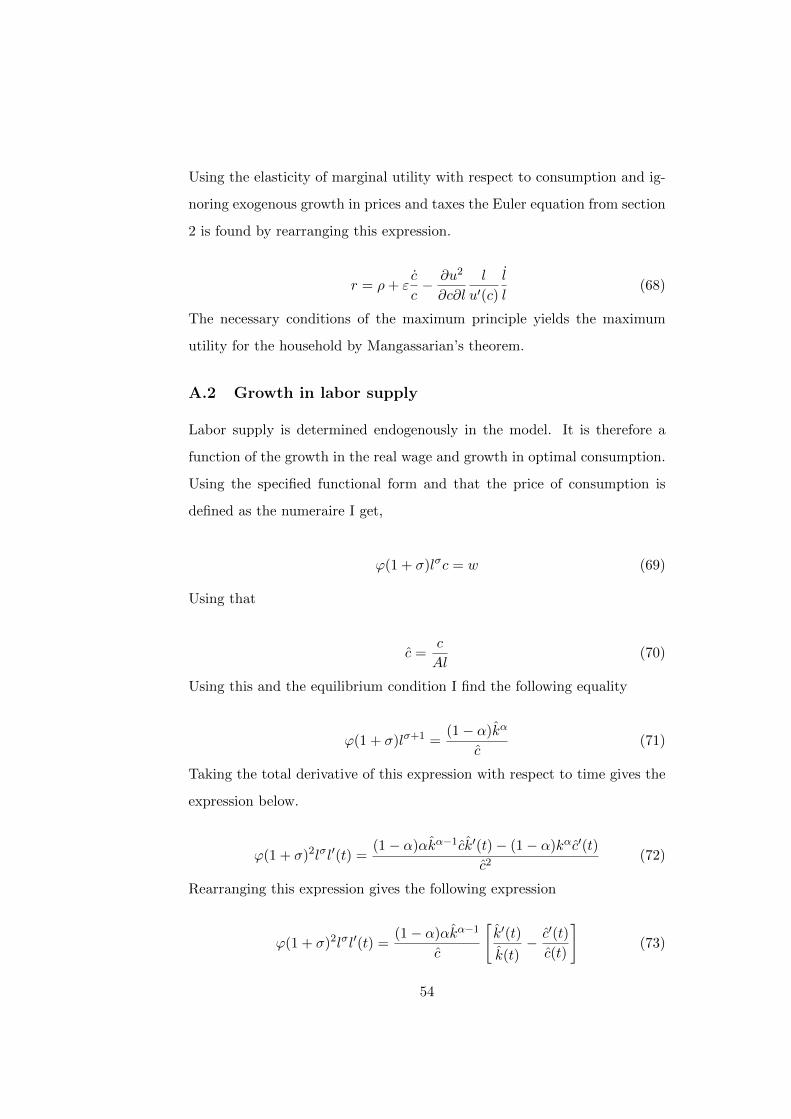
Using the elasticity of marginal utility with respect to consumption and ig-
noring exogenous growth in prices and taxes the Euler equation from section
2 is found by rearranging this expression.
r = ρ+ εc
c− ∂u2
∂c∂l
l
u′(c)
l
l(68)
The necessary conditions of the maximum principle yields the maximum
utility for the household by Mangassarian’s theorem.
A.2 Growth in labor supply
Labor supply is determined endogenously in the model. It is therefore a
function of the growth in the real wage and growth in optimal consumption.
Using the specified functional form and that the price of consumption is
defined as the numeraire I get,
ϕ(1 + σ)lσc = w (69)
Using that
c =c
Al(70)
Using this and the equilibrium condition I find the following equality
ϕ(1 + σ)lσ+1 =(1 − α)kα
c(71)
Taking the total derivative of this expression with respect to time gives the
expression below.
ϕ(1 + σ)2lσl′(t) =(1 − α)αkα−1ck′(t) − (1 − α)kαc′(t)
c2(72)
Rearranging this expression gives the following expression
ϕ(1 + σ)2lσl′(t) =(1 − α)αkα−1
c
[k′(t)
k(t)− c′(t)
c(t)
](73)
54

Using that,
ϕ(1 + σ)lσ+1 =(1 − α)kα
c(74)
I find the expression below by rearranging
l
l=
α
1 + σ
˙k
k− 1
1 + σ
˙c
c(75)
A.3 A solution to the firm’s problem
The Hamilton function of the problem is given by the following expression,
H(t,K, µ, r, w) = f(K,L) − I − wL]e−rt + µ(t)(I − δK) (76)
Maximizing with respect to I yields,
µ(t) = e−rt. (77)
Further,
µ′(t) = −H ′(K) = −e−rtf ′(K) + µ(t)δ (78)
Taking the derivative of the first expression and inserting yields,
−re−rt = −e−rtf ′(K) + δe−rt (79)
This condition gives the optimal capital function K∗(t) that maximizes
the problem for a given function of labor demand. Finding the labor demand
is then like a static problem an amounts to maximizing the profit for each
time t.
A.4 The growth rate of capital per efficient capita
The aggregate resource constraint is found by combining the equilibrium
conditions with the consumers budget constraint.
55

k = rk + wl − pc (80)
Again using the definition of the per efficient capita formulation of capital
k =k
Al(81)
Taking the derivative of this expression gives,
˙k =
kAl − [kAl + kAl]
(Al)2(82)
Inserting for k gives the following expression
˙k =
rk + wl − c
Al− k
[x+
l
l
](83)
Using the equilibrium conditions and rearranging I get the equation for the
growth rate of capital in the text.
˙k
k= kα−1 −
[δ + x+
l
l
]− c
k(84)
Using the expression for the growth rate of labor the above expression can
be reduced further. I will however abstain for this because I do not need
the reduced form equation for the growth in capital for my applications.
A.5 The firm’s problem with non-neutral taxation of profits
For simplicity I rewrite
(1 − τ)(f(K,L) − sI − wL) − (1 − s)I (85)
to
(1 − τ)(f(K,L) − wL) − (1 − sτ)I. (86)
56

As already noted, the present value hamiltonian can not be used in a general
equilibrium setting. I therefore formulate the problem as in the firm’s prob-
lem above. Maximizing the hamilton function with respect to the control
yields the following equation,
µ(t) = e−rt(1 − sτ), (87)
where µ(t) is the costate function of the problem. Then I use the following
first order condition,
µ′(t) = µ(t)δ − e−rt(1 − τ)f ′(k). (88)
Taking the derivative of the first first order condition with respect to time
yields the following equation,
µ′(t) = −re−rt(1 − sτ). (89)
Inserting and rearranging yields the following expression,
−re−rt(1 − sτ) = δe−rt(1 − sτ) − e−rt(1 − τ)f ′(k). (90)
Solving this for the marginal product of k yields the following expression,
f ′(k) =(1 − sτ)
(1 − τ)(δ + r). (91)
In the body of the text I denote,
(1 − sτ)
(1 − τ)=
1
(1 − τf ), (92)
where τf can be interpreted as the effective tax rate on capital on the firm.
Thus,
τf =τ(1 − s)
1 − st. (93)
57

When s=1 it is clear that the effective tax rate is zero. In this case all costs
are deducted from the profits and this case therefore amounts to the well
known property that taxation of pure rents is neutral. Decreases in s drives
a wedge between the real and private return of capital from the viewpoint
of the firm.
A.6 Growth rates in consumption and capital
By combining the equations on growth rate in capital, consumption and
labor supply it is possible to find the growth rate in consumption and capital
expressed only by exogenous variables. The three equations are given by the
following expressions as elaborated upon above.
˙k
k= kα−1 −
[δ + x+
l
l
]− c
k(94)
˙c
c= αkα−1 − (δ + ρ+ x) − l
l(95)
l
l=
α
1 + σ
˙k
k− 1
1 + σ
˙c
c(96)
By inserting the growth rate of labor supply into the growth rate of capital
and consumption and then combining these two expressions.
A.7 Steady state
The steady state values of the system are found by solving the system below.
0 = kα−1 − [δ + x] − c
k(97)
0 = αkα−1 − (δ + ρ+ x) (98)
ϕ(1 + σ)lσ+1 =(1 − α)kα
c(99)
58

This is a well defined system of three equations and three unknowns. This
gives the steady state value of all the endogenous variables that are displayed
in the body of the text in section two.
A.8 Production efficiency
Equalizing tax rates on capital is done to impact the production efficiency
of the economy. Having mentioned this several times, this will be elaborated
upon in this subsection in a more general setting that in the model of section
2.
Taxation of firms’ profits distorts the demand for capital, inducing the
overall level of investment, and therefore the capital intensity to become
inefficiently low. However, taxing capital differently for different firms also
causes static distortions in the market for capital. This could happen if
a lower tax rate is levied on firms that are not incorporated. This could
change the cost of the various inputs for different firms, if the corporate in-
come tax is not neutral. This can be illustrated using the model by levying
two different tax rates on profits for firms that in some way differ. The first
order conditions of these firms are given below.
p1f′1(K) =
r
1 − τ1p1f′1(L) = w
p2f′2(K) =
r
1 − τ2p2f′2(L) = w
These equations can be combined to yield the condition for production effi-
ciency.
f ′1(K)f ′1(l)
f ′2(K)f ′2(l)
=1 − τ2
1 − τ1(100)
The first best allocation is characterized by the following equality.
59

f ′1(K)f ′1(l)
f ′2(K)f ′2(l)
= 1 (101)
This results in a tax induced wedge on the productive efficiency in the case
of corporate taxation that is proportional to the difference in the tax rates
on the two firms. The right hand side of this expression is the ratio of the
marginal willingness to pay labor for an additional unit of capital in the
corporated and unincorporated sector. Since the ratio is less than one, the
corporate sector values an additional unit of capital more than the unin-
corporated sector. Thus, pareto-improving trades between the sectors are
possible, but the corporate tax rate prevents these trades from taking place.
This shows that corporate taxation has an additional harmful effect on the
equilibrium allocation of capital also within each period. Taxing all types of
capital equal to the corporate tax rate may alleviate this distortion. Thus
taxing different organizational forms of firms more equal will realize produc-
tion efficiency. As can be seen above, this will remove all the intratemporal
distortions in the capital markets of the model. This is taking the economy
back to the first best allocation of capital and labor in the intratemporal
equilibrium. The productive capacity of the economy could then be in-
creased by using resources more efficiently.
60

B
Empirical appendix
B.1 Testing for robustness of the results
In this section I estimate the same relationship using a random effects model.
The estimates are reported in table 4. The estimates on the control coef-
ficients are less stable over the different specifications and less as expected
from economic theory. However, the DIT variable remains positive and sig-
nificant. The effect of including data on corporate income taxation remains
the same as in the fixed effects approach.
B.2 Testing for unit roots in a panel data setting
It is well known that many time series on aggregate macroeconomic data
are not stationary, they thus follow a random walk, (Davidson and Mackin-
non (2009)). This has consequences for the interpretation of the estimated
parameters of the econometric model. If there is a presence os a unit root in
some of the variables of the panel this might result in spurious regressions,
estimating a positive and significant result that is completely a result of the
random walk of the time series. In addition the estimates of coefficients do
not follow the standard t-distribution. Rather it follows the Dickey-Fuller
distribution. This has potential consequences for the inference that can be
done with the estimated model and needs to be taken account of. I find
strong evidence that all the series are either integrated to order one or zero
using the Dickey-Fuller test for panel data. The logarithm of unemployment
show strong signs of unit roots. Conducting the same test for this variable
with the first difference I find that there is a strong indication that the series
is integrated of the first order. This is taken account for in the specification
of the model by using the differenced series.
61

Table 4: Estimation with OLS
Dependent variable:
Log GDP per capita (1) (2) (3) (4) (5)
Baseline model
Capital stock .023 .04 .049 .039
(.001) (.004) (.008) (.003) (.003)
Human capital .07 -3.64 -2.87 -3.50 -3.28
(.130) (.27) (.37) (.249) (.207)
Population growth -.069 -.56 -.27 -.531 -.515
(.035) (.18) (.262) (.163) (.133)
Control variables
∆LogUnemployment rate -.033 .075 .0151 .47
(.32) (.24) (.29) (.243)
R&D intensity 1.7 -.185 -.683 -2.76
(1.69) (2.33) (1.57) (.291)
Inflation .02 .0001 .054 .040
(.030) (.003) (.027) (.022)
Saving rate .001 .023 .002 ..004
(.012) (.018) (.011) (.009)
FDI -2.00 e-6 -1.8e-7 -1.54e-6 -6.23e-7
(.000) (.000) (.000) (.000)
Terms of trade -.02 -0.18 -.025 -.020
(.004) (.006) (.004) (.003)
Tax variables
Average tax wedge .009
(.008)
Corporate income tax -4.64 -4.72
(1.32) (.697)
DIT .508 .24
(.09) (.017)
Number of observations: 208 103 56 103 103
R2 overall: 0.26 0.96 0.98 0.95 0.97
Note: All the coefficients are estimated using country random effects. Standard errors are in
brackets.
62