a the simplex solution method - winonacourse1.winona.edu/mwolfmeyer/ba340/module_a.pdf · only...

AThe Simplex Solution Method

A-1

Karen Goldsmith

Converting the Model into Standard Form

The first step in solving a linear programming model manually with the simplex method isto convert the model into standard form. At the Beaver Creek Pottery Company NativeAmerican artisans produce bowls (x1) and mugs (x2) from labor and clay. The linear pro-gramming model is formulated as

maximize Z � $40x1 � 50x2 (profit)

subject to

x1 � 2x2 � 40 (labor, hr)4x1 � 3x2 � 120 (clay, lb)

x1, x2 � 0

We convert this model into standard form by adding slack variables to each constraintas follows.

maximize Z � 40x1 � 50x2 � 0s1 � 0s2

A-2 Module A The Simplex Solution Method

The simplex method, is a general mathematical solution technique for solving linearprogramming problems. In the simplex method, the model is put into the form of atable, and then a number of mathematical steps are performed on the table. These

mathematical steps in effect replicate the process in graphical analysis of moving from oneextreme point on the solution boundary to another. However, unlike the graphical method,in which we could simply search through all the solution points to find the best one, thesimplex method moves from one better solution to another until the best one is found, andthen it stops.

The manual solution of a linear programming model using the simplex method can bea lengthy and tedious process. Years ago, manual application of the simplex method was theonly means for solving a linear programming problem. Now computer solution is certainlypreferred. However, knowledge of the simplex method can greatly enhance one’s under-standing of linear programming. Computer software programs like QM for Windows orExcel spreadsheets provide solutions to linear programming problems, but they do notconvey an in-depth understanding of how those solutions are derived. To a certain extent,graphical analysis provides an understanding of the solution process, and knowledge of thesimplex method further expands on that understanding. In fact, computer solutions areusually derived using the simplex method. As a result, much of the terminology and nota-tion used in computer software comes from the simplex method. Thus, for those studentsof management science who desire a more in-depth knowledge of linear programming, it isbeneficial to study the simplex solution method as provided here.

Converting the Model into Standard Form A-3

Slack variables are added to �constraints and represent

unused resources.

subject to

x1 � 2x2 � s1 � 404x1 � 3x2 � s2 � 120

x1, x2, s1, s2 � 0

The slack variables, s1 and s2, represent the amount of unused labor and clay, respectively.For example, if no bowls and mugs are produced, and x1 � 0 and x2 � 0, then the solutionto the problem is

x1 � 2x2 � s1 � 400 � 2(0) � s1 � 40

s1 � 40 hr of labor

and

4x1 � 3x2 � s2 � 1204(0) � 3(0) � s2 � 120

s2 � 120 lb of clay

In other words, when we start the problem and nothing is being produced, all the resourcesare unused. Since unused resources contribute nothing to profit, the profit is zero.

Z � $40x1 � 50x2 � 0s1 � 0s2� 40(0) � 50(0) � 0(40) � 0(120)

Z � $0

It is at this point that we begin to apply the simplex method. The model is in therequired form, with the inequality constraints converted to equations for solution with thesimplex method.

Once both model constraints have been transformed into equations, the equations shouldbe solved simultaneously to determine the values of the variables at every possible solutionpoint. However, notice that our example problem has two equations and four unknowns(i.e., two decision variables and two slack variables), a situation that makes direct simulta-neous solution impossible. The simplex method alleviates this problem by assigning someof the variables a value of zero. The number of variables assigned values of zero is n � m,where n equals the number of variables and m equals the number of constraints (excludingthe nonnegativity constraints). For this model, n � 4 variables and m � 2 constraints;therefore, two of the variables are assigned a value of zero (i.e., 4 � 2 � 2).

For example, letting x1 � 0 and s1 � 0 results in the following set of equations.

x1 � 2x2 � s1 � 404x1 � 3x2 � s2 � 120

and

0 � 2x2 � 0 � 400 � 3x2 � s2 � 120

First, solve for x2 in the first equation:

2x2 � 40x2 � 20

The Solution of Simultaneous Equations


Figure A-1

Solutions at points A, B, and C

10

100

x1

x2

20 30 40

20

30

40

A

B

C

4x1 + 3x2 + s2 = 120

x1 + 2x

2 + s1 = 40 x1 = 30

x2 = 0s1 = 10s2 = 0

x1 = 0x2 = 20s1 = 0s2 = 60

x1 = 24x2 = 8s1 = 0s2 = 0

Then, solve for s2 in the second equation:

3x2 � s2 � 1203(20) � s2 � 120

s2 � 60

This solution corresponds with point A in Figure A-1. The graph in Figure A-1 showsthat at point A, x1 � 0, x2 � 20, s1 � 0, and s2 � 60, the exact solution obtained by solvingsimultaneous equations. This solution is referred to as a basic feasible solution. A feasiblesolution is any solution that satisfies the constraints. A basic feasible solution satisfies theconstraints and contains as many variables with nonnegative values as there are model con-straints—that is, m variables with nonnegative values and n � m values set equal to zero.Typically, the m variables have positive nonzero solution values; however, when one of them variables equals zero, the basic feasible solution is said to be degenerate. (The topic ofdegeneracy will be discussed at a later point in this module.)

Consider a second example where x2 � 0 and s2 � 0. These values result in the follow-ing set of equations.

x1 � 2x2 � s1 � 404x1 � 3x2 � s2 � 120

andx1 � 0 � s1 � 40

4x1 � 0 � 0 � 120

Solve for x1:4x1 � 120

x1 � 30Then solve for s1:

30 � s1 � 40s1 � 10

This basic feasible solution corresponds to point C in Figure A-1, where x1 � 30, x2 � 0,s1 � 10, and s2 � 0.

A basic feasible solution satisfiesthe model constraints and has the

same number of variables withnon-negative values as there are

constraints.

The Simplex Method A-5

The Simplex Method

Finally, consider an example where s1 � 0 and s2 � 0. These values result in the follow-ing set of equations.

x1 � 2x2 � s1 � 404x1 � 3x2 � s2 � 120

and

x1 � 2x2 � 0 � 404x1 � 3x2 � 0 � 120

These equations can be solved using row operations. In row operations, the equationscan be multiplied by constant values and then added or subtracted from each other with-out changing the values of the decision variables. First, multiply the top equation by 4 toget

4x1 � 8x2 � 160

and then subtract the second equation:

4x1 � 8x2 � 160�4x1 � 3x2 � �120

5x2 � 40x2 � 8

Next, substitute this value of x2 into either one of the constraints.

x1 � 2(8) � 40x1 � 24

This solution corresponds to point B on the graph, where x1 � 24, x2 � 8, s1 � 0, ands2 � 0, which is the optimal solution point.

All three of these example solutions meet our definition of basic feasible solutions.However, two specific questions are raised by the identification of these solutions.

1. In each example, how was it known which variables to set equal to zero?2. How is the optimal solution identified?

The answers to both of these questions can be found by using the simplex method. Thesimplex method is a set of mathematical steps that determines at each step which variablesshould equal zero and when an optimal solution has been reached.

Row operations are used to solvesimultaneous equations where

equations are multiplied by con-stants and added or subtracted

from each other.

The steps of the simplex method are carried out within the framework of a table, ortableau. The tableau organizes the model into a form that makes applying the mathemat-ical steps easier. The Beaver Creek Pottery Company example will be used again to demon-strate the simplex tableau and method.

maximize Z � $40x1 � 50x2 � 0s1 � 0s2

subject to

x1 � 2x2 � s1 � 40 hr4x1 � 3x2 � s2 � 120 lb

x1, x2, s1, s2 � 0

The simplex method is a set ofmathematical steps for solving

a linear programming problemcarried out in a table called a

simplex tableau.

The first step in filling in Table A-1 is to record the model variables along the second rowfrom the top. The two decision variables are listed first, in order of their subscript magni-tude, followed by the slack variables, also listed in order of their subscript magnitude. Thisstep produces the row with x1, x2, s1, and s2 in Table A-1.

The next step is to determine a basic feasible solution. In other words, which two vari-ables will form the basic feasible solution and which will be assigned a value of zero?Instead of arbitrarily selecting a point (as we did with points A, B, and C in the previoussection), the simplex method selects the origin as the initial basic feasible solution becausethe values of the decision variables at the origin are always known in all linear programmingproblems. At that point x1 � 0 and x2 � 0; thus, the variables in the basic feasible solutionare s1 and s2.

x1 � 2x2 � s1 � 400 � 2(0) � s1 � 40

s1 � 40 hr

and

4x1 � 3x2 � s2 � 1204(0) � 3(0) � s2 � 120

s2 � 120 lb

In other words, at the origin, where there is no production, all resources are slack, orunused. The variables s1 and s2, which form the initial basic feasible solution, are listed inTable A-2 under the column “Basic Variables,” and their respective values, 40 and 120, arelisted under the column “Quantity.”


Basiccj Variables Quantity x1 x2 s1 s2

s1 40

s2 120

zj

cj � zj

Table A-2The Basic Feasible Solution

Basiccj Variables Quantity x1 x2 s1 s2

zj

cj � zj

Table A-1The Simplex Tableau

The initial simplex tableau for this model, with the various column and row headings, isshown in Table A-1.

The basic feasible solution in theinitial simplex tableau is the origin

where all decision variablesequal zero.

At the initial basic feasible solutionat the origin, only slack variables

have a value greater than zero.


Basic40 50 0 0

cj Variables Quantity x1 x2 s1 s2

0 s1 40

0 s2 120

zj

cj � zj

Table A-3The Simplex Tableau with

cj Values

Basic40 50 0 0


0 s1 40 1 2 1 0

0 s2 120 4 3 0 1

zj

cj � zj

Table A-4The Simplex Tableau with

Model Constraint Coefficients

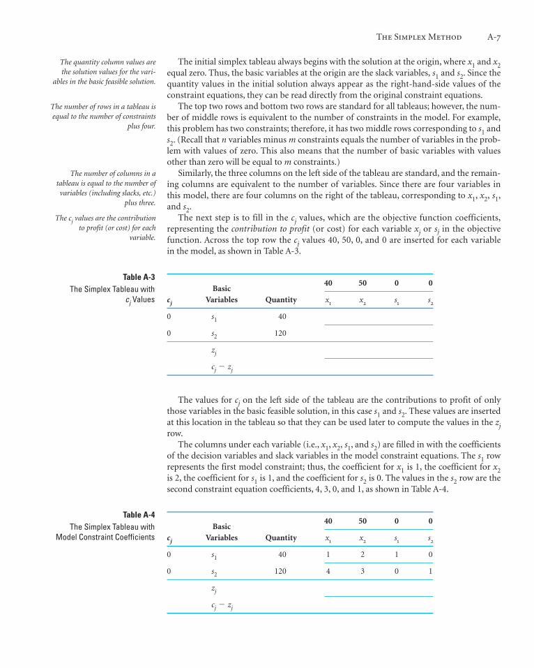
The initial simplex tableau always begins with the solution at the origin, where x1 and x2equal zero. Thus, the basic variables at the origin are the slack variables, s1 and s2. Since thequantity values in the initial solution always appear as the right-hand-side values of theconstraint equations, they can be read directly from the original constraint equations.

The top two rows and bottom two rows are standard for all tableaus; however, the num-ber of middle rows is equivalent to the number of constraints in the model. For example,this problem has two constraints; therefore, it has two middle rows corresponding to s1 ands2. (Recall that n variables minus m constraints equals the number of variables in the prob-lem with values of zero. This also means that the number of basic variables with valuesother than zero will be equal to m constraints.)

Similarly, the three columns on the left side of the tableau are standard, and the remain-ing columns are equivalent to the number of variables. Since there are four variables inthis model, there are four columns on the right of the tableau, corresponding to x1, x2, s1,and s2.

The next step is to fill in the cj values, which are the objective function coefficients,representing the contribution to profit (or cost) for each variable xj or sj in the objectivefunction. Across the top row the cj values 40, 50, 0, and 0 are inserted for each variablein the model, as shown in Table A-3.

The quantity column values arethe solution values for the vari-

ables in the basic feasible solution.

The number of rows in a tableau isequal to the number of constraints

plus four.

The number of columns in atableau is equal to the number ofvariables (including slacks, etc.)

plus three.

The values for cj on the left side of the tableau are the contributions to profit of onlythose variables in the basic feasible solution, in this case s1 and s2. These values are insertedat this location in the tableau so that they can be used later to compute the values in the zjrow.

The columns under each variable (i.e., x1, x2, s1, and s2) are filled in with the coefficientsof the decision variables and slack variables in the model constraint equations. The s1 rowrepresents the first model constraint; thus, the coefficient for x1 is 1, the coefficient for x2is 2, the coefficient for s1 is 1, and the coefficient for s2 is 0. The values in the s2 row are thesecond constraint equation coefficients, 4, 3, 0, and 1, as shown in Table A-4.

The cj values are the contributionto profit (or cost) for each

variable.


Basic40 50 0 0


0 s1 40 1 2 1 0

0 s2 120 4 3 0 1

zj 0 0 0 0 0

cj � zj

Table A-5The Simplex Tableau with zj

Row Values

This completes the process of filling in the initial simplex tableau. The remaining valuesin the zj and cj � zj rows, as well as subsequent tableau values, are computed mathemat-ically using simplex formulas.

The following list summarizes the steps of the simplex method (for a maximizationmodel) that have been presented so far.

1. First, transform all inequalities to equations by adding slack variables.2. Develop a simplex tableau with the number of columns equaling the number of

variables plus three, and the number of rows equaling the number of constraints plusfour.

3. Set up table headings that list the model decision variables and slack variables.4. Insert the initial basic feasible solution, which are the slack variables and their quan-

tity values.5. Assign cj values for the model variables in the top row and the basic feasible solution

variables on the left side.6. Insert the model constraint coefficients into the body of the table.

So far the simplex tableau has been set up using values taken directly from the model. Fromthis point on the values are determined by computation. First, the values in the zj row arecomputed by multiplying each cj column value (on the left side) by each column valueunder Quantity, x1, x2, s1, and s2 and then summing each of these sets of values. The zjvalues are shown in Table A-5.

Computing the zj and cj � zj RowsThe zj row values are computed by

multiplying the cj column valuesby the variable column values

and summing.

For example, the value in the zj row under the quantity column is found as follows.

cj Quantity

0 � 40 � 00 � 120 � 0

zq � 0

The value in the zj row under the x1 column is found similarly.

cj x1

0 � 1 � 00 � 4 � 0

zj � 0

All of the other zj row values for this tableau will be zero when they are computed using thisformula.

Now the cj � zj row is computed by subtracting the zj row values from the cj (top) rowvalues. For example, in the x1 column the cj � zj row value is computed as 40 � 0 � 40.

The simplex method works bymoving from one solution

(extreme) point to an adjacentpoint until it locates the best

solution.


Basic40 50 0 0


0 s1 40 1 2 1 0

0 s2 120 4 3 0 1

zj 0 0 0 0 0

cj � zj 40 50 0 0

Table A-6The Complete Initial

Simplex Tableau

This value as well as other cj � zj values are shown in Table A-6, which is the complete ini-tial simplex tableau with all values filled in. This tableau represents the solution at the ori-gin, where x1 � 0, x2 � 0, s1 � 40, and s2 � 120. The profit represented by this solution(i.e., the Z value) is given in the zj row under the quantity column—0 in Table A-6. Thissolution is obviously not optimal because no profit is being made. Thus, we want to moveto a solution point that will give a better solution. In other words, we want to produce eithersome bowls (x1) or some mugs (x2). One of the nonbasic variables (i.e., variables not in thepresent basic feasible solution) will enter the solution and become basic.

The Entering NonbasicVariable

As an example, suppose the pottery company decides to produce some bowls. With thisdecision x1 will become a basic variable. For every unit of x1 (i.e., each bowl) produced,profit will be increased by $40 because that is the profit contribution of a bowl. How-ever, when a bowl (x1) is produced, some previously unused resources will be used. Forexample, if

x1 � 1

then

x1 � 2x2 � s1 � 40 hr of labor1 � 2(0) � s1 � 40

s1 � 39 hr of labor

and

4x1 � 3x2 � s2 � 120 lb of clay4(1) � 3(0) � s2 � 120

s2 � 116 lb of clay

In the labor constraint we see that, with the production of one bowl, the amount ofslack, or unused, labor is decreased by 1 hour. In the clay constraint the amount of slack isdecreased by 4 pounds. Substituting these increases (for x1) and decreases (for slack) intothe objective function gives

cj zj

Z � 40(1) � 50(0) � 0(�1) � 0(�4)Z � $40

The first part of this objective function relationship represents the values in the cj row;the second part represents the values in the zj row. The function expresses the fact that toproduce some bowls, we must give up some of the profit already earned from the itemsthey replace. In this case the production of bowls replaced only slack, so no profit was lost.In general, the cj � zj row values represent the net increase per unit of entering a nonbasic

The variable with the largestpositive cj � zj value is the

entering variable.

Basic40 50 0 0


0 s1 40 1 2 1 0

0 s2 120 4 3 0 1

zj 0 0 0 0 0

cj � zj 40 50 0 0


Table A-7Selection of the Entering Basic

Variable

Figure A-2

Selection of which item toproduce — the entering basic

variable

10

100

x1

x2

20 30 40

20

30

40

A

B

C

Pro

duce

mug

s

Produce bowls

variable into the basic solution. Naturally, we want to make as much money as possible,because the objective is to maximize profit. Therefore, we enter the variable that will givethe greatest net increase in profit per unit. From Table A-7, we select variable x2 as theentering basic variable because it has the greatest net increase in profit per unit, $50 — thehighest positive value in the cj � zj row.

The x2 column, highlighted in Table A-7, is referred to as the pivot column. (The opera-tions used to solve simultaneous equations are often referred to in mathematical termin-ology as pivot operations.)

The selection of the entering basic variable is also demonstrated by the graph inFigure A-2. At the origin nothing is produced. In the simplex method we move from onesolution point to an adjacent point (i.e., one variable in the basic feasible solution isreplaced with a variable that was previously zero). In Figure A-2 we can move along eitherthe x1 axis or the x2 axis in order to seek a better solution. Because an increase in x2 willresult in a greater profit, we choose x2.

The pivot column is the columncorresponding to the entering

variable.

Since each basic feasible solution contains only two variables with nonzero values, one ofthe two basic variables present, s1 or s2, will have to leave the solution and become zero.Since we have decided to produce mugs (x2), we want to produce as many as possible or, inother words, as many as our resources will allow. First, in the labor constraint we will use all

The Leaving Basic Variable


Figure A-3

Determination of the basicfeasible solution point

10

100

x1

x2

20 30 40

20

30

40

A

B

C

$50

prof

it

$40 profit

R

the labor to make mugs (because no bowls are to be produced, x1 � 0; and because we willuse all the labor possible and s1 � unused labor resources, s1 � 0 also).

1x1 � 2x2 � s1 � 40 hr1(0) � 2x2 � 0 � 40

x2 �

� 20 mugs

In other words, enough labor is available to produce 20 mugs. Next, perform the sameanalysis on the constraint for clay.

4x1 � 3x2 � s2 � 120 lb4(0) � 3x2 � 0 � 120

x2 �

� 40 mugs

This indicates that there is enough clay to produce 40 mugs. But there is enough labor to pro-duce only 20 mugs. We are limited to the production of only 20 mugs because we do not haveenough labor to produce any more than that. This analysis is shown graphically in Figure A-3.

120 lb

3 lb/mug

40 hr

2 hr/mug

Because we are moving out the x2 axis, we can move from the origin to either point A orpoint R. We select point A because it is the most constrained and thus feasible, whereas pointR is infeasible.

This analysis is performed in the simplex method by dividing the quantity values of thebasic solution variables by the pivot column values. For this tableau,

BasicVariables Quantity x2

s1 40 ÷ 2 � 20, the leaving basic variables2 120 ÷ 3 � 40

The leaving variable is determinedby dividing the quantity values by

the pivot column values andselecting the minimum possible

value or zero.


Table A-8Pivot Column, Pivot Row, and

Pivot Number

Basic40 50 0 0


50 x2

0 s2

zj

cj � zj

Table A-9The Basic Variables and cj

Values for the SecondSimplex Tableau

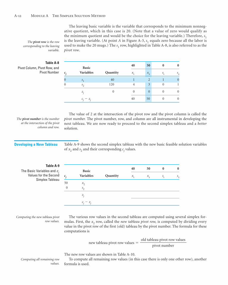
The leaving basic variable is the variable that corresponds to the minimum nonneg-ative quotient, which in this case is 20. (Note that a value of zero would qualify asthe minimum quotient and would be the choice for the leaving variable.) Therefore, s1is the leaving variable. (At point A in Figure A-3, s1 equals zero because all the labor isused to make the 20 mugs.) The s1 row, highlighted in Table A-8, is also referred to as thepivot row.

The value of 2 at the intersection of the pivot row and the pivot column is called thepivot number. The pivot number, row, and column are all instrumental in developing thenext tableau. We are now ready to proceed to the second simplex tableau and a bettersolution.

Table A-9 shows the second simplex tableau with the new basic feasible solution variablesof x2 and s2 and their corresponding cj values.

The pivot row is the rowcorresponding to the leaving

variable.

The pivot number is the numberat the intersection of the pivot

column and row.

Developing a New Tableau

Computing the new tableau pivotrow values.

The various row values in the second tableau are computed using several simplex for-mulas. First, the x2 row, called the new tableau pivot row, is computed by dividing everyvalue in the pivot row of the first (old) tableau by the pivot number. The formula for thesecomputations is

new tableau pivot row values �

The new row values are shown in Table A-10.To compute all remaining row values (in this case there is only one other row), another

formula is used.

old tableau pivot row values

pivot number

Computing all remaining rowvalues.

Basic40 50 0 0


0 s1 40 1 2 1 0

0 s2 120 4 3 0 1

zj 0 0 0 0 0

cj � zj 40 50 0 0


Basic40 50 0 0


50 x2 20 1/2 1 1/2 0

0 s2

zj

cj � zj

Table A-10Computation of the New Pivot

Row Values

Quantity 120 � (3 � 20) � 60

x1 4 � (3 � 1/2) � 5/2

x2 3 � (3 � 1) � 0

s1 0 � (3 � 1/2) � �3/2

s2 1 � (3 � 0) � 1

Column

Old Tableau

Row Value

� �Corresponding

Coefficients in

Pivot Column

�

New Tableau

Pivot

Row Value � � New Tableau

Row Value

Table A-11Computation of New s2

Row Values

Basic40 50 0 0


50 x2 20 1/2 1 1/2 0

0 s2 60 5/2 0 �3/2 1

zj

cj � zj

Table A-12The Second Simplex Tableau

with Row Values

Thus, this formula requires the use of both the old tableau and the new one. The s2 rowvalues are computed in Table A-11.

new tableaurow values �

old tableaurow values � �corresponding

coefficients inpivot column

�corresponding

new tableaupivot row value�

These values have been inserted in the simplex tableau in Table A-12.This solution corresponds to point A in the graph of this model in Figure A-3. The solu-

tion at this point is x1 � 0, x2 � 20, s1 � 0, s2 � 60. In other words, 20 mugs are producedand 60 pounds of clay are left unused. No bowls are produced and no labor hours remainunused.

The second simplex tableau is completed by computing the zj and cj � zj row values thesame way they were computed in the first tableau. The zj row is computed by summing theproducts of the cj column and all other column values.


After developing the simplex method for solving linear pro-gramming problems, George Dantzig needed a good problemto test it on. The problem he selected was the “diet problem”formulated in 1945 by Nobel economist George Stigler. Thisproblem was to determine an adequate nutritional diet at min-imum cost (which was an important military and civilian issueduring World War II). Formulated as a linear programming

model, the diet problem consisted of 77 unknowns and 9 equa-tions. It took 9 clerks using hand-operated (mechanical) deskcalculators 120 man-days to obtain the optimal simplex solu-tion: a diet consisting primarily of wheat flour, cabbage, anddried navy beans that cost $39.69 per year (in 1939 prices). Thesolution developed by Stigler using his own numerical methodwas only 24 cents more than the optimal solution.

for George B. DantzigTime Out

Basic40 50 0 0


50 x2 20 1/2 1 1/2 0

0 s2 60 5/2 0 �3/2 1

zj 1,000 25 50 25 0

cj � zj 15 0 �25 0

Table A-13The Completed Second

Simplex Tableau

Column

Quantity zj � (50) (20) � (0) (60) � 1000x1 z1 � (50) (1/2) � (0) (5/2) � 25x2 z2 � (50) (1) � (0) (0) � 50s1 z3 � (50) (1/2) � (0) (�3/2) � 25s2 z4 � (50) (0) � (0) (1) � 0

The zj row values and the cj � zj row values are added to the tableau to give the com-pleted second simplex tableau shown in Table A-13. The value of 1,000 in the zj row is thevalue of the objective function (profit) for this basic feasible solution.

Each tableau is the same as per-forming row operations for a set of

simultaneous equations.

The computational steps that we followed to derive the second tableau in effect accom-plish the same thing as row operations in the solution of simultaneous equations. Thesesame steps are used to derive each subsequent tableau, called iterations.

The steps that we followed to derive the second simplex tableau are repeated to develop thethird tableau. First, the pivot column or entering basic variable is determined. Because 15 in the cj � zj row represents the greatest positive net increase in profit, x1 becomes theentering nonbasic variable. Dividing the pivot column values into the values in the quantitycolumn indicates that s2 is the leaving basic variable and corresponds to the pivot row. Thepivot row, pivot column, and pivot number are indicated in Table A-14.

At this point you might be wondering why the net increase in profit per bowl (x1) is $15rather than the original profit of $40. It is because the production of bowls (x1) will requiresome of the resources previously used to produce mugs (x2) only. Producing some bowlsmeans not producing as many mugs; thus, we are giving up some of the profit gained fromproducing mugs to gain even more by producing bowls. This difference is the net increaseof $15.

The Optimal SimplexTableau


Table A-14The Pivot Row, Pivot Column,

and Pivot Number

Quantity 20 � (1/2 � 24) � 8

x1 1/2 � (1/2 � 1) � 0

x2 1 � (1/2 � 0) � 1

s1 1/2 � (1/2 � �3/5) � 4/5

s2 0 � (1/2 � 2/5) � �1/5

Column

Old Tableau

Row Value

� �Corresponding

Coefficients in

Pivot Column

�

New Tableau

Pivot

Row Value � � New Tableau

Row Value

Table A-15Computation of the x2 Row for

the Third Simplex Tableau

Basic40 50 0 0


50 x2 8 0 1 4/5 �1/5

40 x1 24 1 0 �3/5 2/5

zj 1,360 40 50 16 6

cj � zj 0 0 �16 �6

Table A-16The Completed Third Simplex

Tableau

The new tableau pivot row (x1) in the third simplex tableau is computed using the sameformula used previously. Thus, all old pivot row values are divided through by 5/2, thepivot number. These values are shown in Table A-16. The values for the other row (x2) arecomputed as shown in Table A-15.

These new row values, as well as the new zj row and cj � zj row, are shown in the com-pleted third simplex tableau in Table A-16.

Observing the cj � zj row to determine the entering variable, we see that a nonbasic vari-able would not result in a positive net increase in profit, as all values in the cj � zj row arezero or negative. This means that the optimal solution has been reached. The solution is

x1 � 24 bowlsx2 � 8 mugsZ � $1,360 profit

The solution is optimal when allcj � zj values � 0.

Basic40 50 0 0


50 x2 20 1/2 1 1/2 0

0 s2 60 5/2 0 �3/2 1

zj 1,000 25 50 25 0

cj � zj 15 0 �25 0


Simplex Solution of a Minimization Problem

Summary of the Simplex Method

which corresponds to point B in Figure A-1.An additional comment should be made regarding simplex solutions in general.

Although this solution resulted in integer values for the variables (i.e., 24 and 8), it is pos-sible to get a fractional solution for decision variables even though the variables reflectitems that should be integers, such as airplanes, television sets, bowls, and mugs. To applythe simplex method, one must accept this limitation.

The simplex method demonstrated in the previous section consists of the following steps.

1. Transform the model constraint inequalities into equations.2. Set up the initial tableau for the basic feasible solution at the origin and compute

the zj and cj � zj row values.3. Determine the pivot column (entering nonbasic solution variable) by selecting the

column with the highest positive value in the cj � zj row.4. Determine the pivot row (leaving basic solution variable) by dividing the quantity

column values by the pivot column values and selecting the row with the minimumnonnegative quotient.

5. Compute the new pivot row values using the formula

6. Compute all other row values using the formula

7. Compute the new zj and cj � zj rows.8. Determine whether or not the new solution is optimal by checking the cj � zj row. If

all cj � zj row values are zero or negative, the solution is optimal. If a positive valueexists, return to step 3 and repeat the simplex steps.

new tableaurow values

�old tableaurow values

� �correspondingcoefficients inpivot Column

�

correspondingnew tableau

pivot row values�

new tableau pivot row values �old tableau pivot row values

pivot number

In the previous section the simplex method for solving linear programming problems wasdemonstrated for a maximization problem. In general, the steps of the simplex methodoutlined at the end of this section are used for any type of linear programming problem.However, a minimization problem requires a few changes in the normal simplex process,which we will discuss in this section.

In addition, several exceptions to the typical linear programming problem will be pre-sented later in this module. These include problems with mixed constraints (�, �, and �);problems with more than one optimal solution, no feasible solution, or an unboundedsolution; problems with a tie for the pivot column; problems with a tie for the pivot row;and problems with constraints with negative quantity values. None of these kinds ofproblems require changes in the simplex method. They are basically unusual results inindividual simplex tableaus that the reader should know how to interpret and work with.

The simplex method does notguarantee integer solutions.

Simplex Solution of a Minimization Problem A-17

Figure A-4

Graph of the fertilizer example

2

4

6

8

10

12

20

4 6 8 10 12 x1

x2

x1 = 0x2 = 0s1 = –16

A

B

C

Standard Form of a Minimization Model

Consider the following linear programming model for a farmer purchasing fertilizer.

minimize Z � $6x1 � 3x2

subject to

2x1 � 4x2 � 16 lb of nitrogen4x1 � 3x2 � 24 lb of phosphate

where

x1 � bags of Super-gro fertilizerx2 � bags of Crop-quick fertilizerZ � farmer’s total cost ($) of purchasing fertilizer

This model is transformed into standard form by subtracting surplus variables from thetwo � constraints as follows.

minimize Z � 6x1 � 3x2 � 0s1 � 0s2

subject to

2x1 � 4x2 � s1 � 164x1 � 3x2 � s1 � 24

x1, x2, s1, s2 � 0

The surplus variables represent the extra amount of nitrogen and phosphate that exceededthe minimum requirements specified in the constraints.

However, the simplex method requires that the initial basic feasible solution be at theorigin, where x1 � 0 and x2 � 0. Testing these solution values, we have

2x1 � 4x2 � s1 � 162(0) � 4(0) � s1 � 16

s1 � �16

The idea of “negative excess pounds of nitrogen” is illogical and violates the nonnegativ-ity restriction of linear programming. The reason the surplus variable does not work isshown in Figure A-4. The solution at the origin is outside the feasible solution space.

Transforming a model intostandard form by subtracting

surplus variables will not workin the simplex method.

To alleviate this difficulty and get a solution at the origin, we add an artificial variable(A1) to the constraint equation,

2x1 � 4x2 � s1 � A1 � 16

The artificial variable, A1, does not have a meaning as a slack variable or a surplus variabledoes. It is inserted into the equation simply to give a positive solution at the origin; we areartificially creating a solution.

2x1 � 4x2 � s1 � A1 � 162(0) � 4(0) � 0 � A1 � 16

A1 � 16

The artificial variable is somewhat analogous to a booster rocket — its purpose is to getus off the ground; but once we get started, it has no real use and thus is discarded. The arti-ficial solution helps get the simplex process started, but we do not want it to end up in theoptimal solution, because it has no real meaning.

When a surplus variable is subtracted and an artificial variable is added, the phosphateconstraint becomes

4x1 � 3x2 � s2 � A2 � 24

The effect of surplus and artificial variables on the objective function must now be con-sidered. Like a slack variable, a surplus variable has no effect on the objective function interms of increasing or decreasing cost. For example, a surplus of 24 pounds of nitrogendoes not contribute to the cost of the objective function, because the cost is determinedsolely by the number of bags of fertilizer purchased (i.e., the values of x1 and x2). Thus, acoefficient of 0 is assigned to each surplus variable in the objective function.

By assigning a “cost” of $0 to each surplus variable, we are not prohibiting it from beingin the final optimal solution. It would be quite realistic to have a final solution that showedsome surplus nitrogen or phosphate. Likewise, assigning a cost of $0 to an artificial variablein the objective function would not prohibit it from being in the final optimal solution.However, if the artificial variable appeared in the solution, it would render the final solu-tion meaningless. Therefore, we must ensure that an artificial variable is not in the finalsolution.

As previously noted, the presence of a particular variable in the final solution is based onits relative profit or cost. For example, if a bag of Super-gro costs $600 instead of $6 andCrop-quick stayed at $3, it is doubtful that the farmer would purchase Super-gro (i.e., x1would not be in the solution). Thus, we can prohibit a variable from being in the final solu-tion by assigning it a very large cost. Rather than assigning a dollar cost to an artificial vari-able, we will assign a value of M, which represents a large positive cost (say, $1,000,000). Thisoperation produces the following objective function for our example:

minimize Z � 6x1 � 3x2 � 0s1 � 0s2 � MA1 � MA2

The completely transformed minimization model can now be summarized as

minimize Z � 6x1 � 3x2 � 0s1 � 0s2 � MA1 � MA2

subject to

2x1 � 4x1 � s1 � A1 � 164x1 � 3x2 � s2 � A2 � 24

x1, x2, s1, s2, A1, A2 � 0


An artificial variable allows foran initial basic feasible solution at

the origin, but it has no realmeaning.

Artificial variables are assigned alarge cost in the objective function

to eliminate them from the finalsolution.

Simplex Solution of a Minimization Problem A-19

Table A-17The Initial Simplex Tableau


The initial simplex tableau for a minimization model is developed the same way as one fora maximization model, except for one small difference. Rather than computing cj � zj inthe bottom row of the tableau, we compute zj � cj, which represents the net per unitdecrease in cost, and the largest positive value is selected as the entering variable and pivotcolumn. (An alternative would be to leave the bottom row as cj � zj and select the largestnegative value as the pivot column. However, to maintain a consistent rule for selecting the pivot column, we will use zj � cj.)

The initial simplex tableau for this model is shown in Table A-17. Notice that A1 andA2 form the initial solution at the origin, because that was the reason for insertingthem in the first place — to get a solution at the origin. This is not a basic feasiblesolution, since the origin is not in the feasible solution area, as shown in Figure A-4.As indicated previously, it is an artificially created solution. However, the simplexprocess will move toward feasibility in subsequent tableaus. Note that across the topthe decision variables are listed first, then surplus variables, and finally artificialvariables.

In Table A-17 the x2 column was selected as the pivot column because 7M � 3 is the largest positive value in the zj � cj row. A1 was selected as the leaving basic variable (andpivot row) because the quotient of 4 for this row was the minimum positive row value.

The second simplex tableau is developed using the simplex formulas presentedearlier. It is shown in Table A-18. Notice that the A1 column has been eliminated in thesecond simplex tableau. Once an artificial variable leaves the basic feasible solution,it will never return because of its high cost, M. Thus, like the booster rocket, it can beeliminated from the tableau. However, artificial variables are the only variables that canbe treated this way.

The Simplex Tableau for a Minimization Problem

The cj � zj row is changed tozj � cj in the simplex tableau for

a minimization problem.

Artificial variables are alwaysincluded as part of the initial basic

feasible solution when they exist.

The third simplex tableau, with x1 replacing A2, is shown in Table A-19. Both the A1 andA2 columns have been eliminated because both variables have left the solution. The x1 row

Once an artificial variable isselected as the leaving variable, it

will never reenter the tableau, so itcan be eliminated.

Basic6 3 0 0 M M

cj Variables Quantity x1 x2 s1 s2 A1 A2

M A1 16 2 4 �1 0 1 0

M A2 24 4 3 0 �1 0 1

zj 40M 6M 7M �M �M M M

zj � cj 6M � 6 7M � 3 �M �M 0 0

Basic6 3 0 0 M

cj Variables Quantity x1 x2 s1 s2 A1

3 x2 4 1/2 1 �1/4 0 0

M A2 12 5/2 0 3/4 �1 1

zj 12M � 12 5M/2 � 3/2 3 �3/4 � 3/M4 �M M

zj � cj 5M/2 � 9/2 0 �3/4 � 3/M4 �M 0


Basic6 3 0 0


3 x2 8 4/3 1 0 �1/3

0 s1 16 10/3 0 1 �4/3

zj 24 4 3 0 �1

zj � cj �2 0 0 �1

Table A-20Optimal Simplex Tableau

Table A-19The Third Simplex Tableau

is selected as the pivot row because it corresponds to the minimum positive ratio of 16. Inselecting the pivot row, the �4 value for the x2 row was not considered because the mini-mum positive value or zero is selected. Selecting the x2 row would result in a negative quan-tity value for s1 in the fourth tableau, which is not feasible.

The fourth simplex tableau, with s1 replacing x1, is shown in Table A-20. Table A-20 isthe optimal simplex tableau because the zj � cj row contains no positive values. The opti-mal solution is

x1 � 0 bags of Super-gros1 � 16 extra lb of nitrogenx2 � 8 bags of Crop-quicks2 � 0 extra lb of phosphateZ � $24, total cost of purchasing fertilizer

To summarize, the adjustments necessary to apply the simplex method to a minimizationproblem are as follows:

1. Transform all � constraints to equations by subtracting a surplus variable and addingan artificial variable.

2. Assign a cj value of M to each artificial variable in the objective function.3. Change the cj � zj row to zj � cj.

Although the fertilizer example model we just used included only � constraints, it ispossible for a minimization problem to have � and � constraints in addition to � con-straints. Similarly, it is possible for a maximization problem to have � and � constraintsin addition to � constraints. Problems that contain a combination of different types ofinequality constraints are referred to as mixed constraint problems.

Simplex Adjustments fora Minimization Problem

Basic6 3 0 0


3 x2 8/5 0 1 �2/5 1/5

6 x1 24/5 1 0 3/10 �2/5

zj 168/5 6 3 3/5 �9/5

zj � cj 0 0 3/5 �9/5

A Mixed Constraint Problem A-21

A Mixed Constraint Problem

A mixed constraint problemincludes a combination of �, �,

and � constraints.

So far we have discussed maximization problems with all � constraints and minimizationproblems with all � constraints. However, we have yet to solve a problem with a mix-ture of �, �, and � constraints. Furthermore, we have not yet looked at a maximizationproblem with a � constraint. The following is a maximization problem with �, �, and� constraints.

A leather shop makes custom-designed, hand-tooled briefcases and luggage. The shopmakes a $400 profit from each briefcase and a $200 profit from each piece of luggage. (Theprofit for briefcases is higher because briefcases require more hand tooling.) The shop hasa contract to provide a store with exactly 30 items per month. A tannery supplies the shopwith at least 80 square yards of leather per month. The shop must use at least this amountbut can order more. Each briefcase requires 2 square yards of leather; each piece of luggagerequires 8 square yards of leather. From past performance, the shop owners know they can-not make more than 20 briefcases per month. They want to know the number of briefcasesand pieces of luggage to produce in order to maximize profit.

This problem is formulated as

maximize Z � $400x1 � 200x2

subject to

x1 � x2 � 30 contracted items2x1 � 8x2 � 80 yd2 of leather

x1 � 20 briefcasesx1, x2 � 0

where x1 � briefcases and x2 � pieces of luggage.The first step in the simplex method is to transform the inequalities into equations. The

first constraint for the contracted items is already an equation; therefore, it is not necessaryto add a slack variable. There can be no slack in the contract with the store because exactly30 items must be delivered. Even though this equation already appears to be in the neces-sary form for simplex solution, let us test it at the origin to see if it meets the startingrequirements.

x1 � x2 � 300 � 0 � 30

0 � 30

Because zero does not equal 30, the constraint is not feasible in this form. Recall that a �constraint did not work at the origin either in an earlier problem. Therefore, an artificialvariable was added. The same thing can be done here.

x1 � x2 � A1 � 30

Now at the origin, where x1 � 0 and x2 � 0,

0 � 0 � A1 � 30A1 � 30

Any time a constraint is initially an equation, an artificial variable is added. However, theartificial variable cannot be assigned a value of M in the objective function of a maximiza-tion problem. Because the objective is to maximize profit, a positive M value would repre-sent a large positive profit that would definitely end up in the final solution. Because an arti-ficial variable has no real meaning and is inserted into the model merely to create an initial

An artificial variable is added toan equality (�) constraint for

standard form.




solution at the origin, its existence in the final solution would render the solution mean-ingless. To prevent this from happening, we must give the artificial variable a large cost con-tribution, or �M.

The constraint for leather is a � inequality. It is converted to equation form by subtract-ing a surplus variable and adding an artificial variable:

2x1 � 8x2 � s1 � A2 � 80

As in the equality constraint, the artificial variable in this constraint must be assigned anobjective function coefficient of �M.

The final constraint is a � inequality and is transformed by adding a slack variable:

x1 � s2 � 20

The completely transformed linear programming problem is as follows:

maximize Z � 400x1 � 200x2 � 0s1 � 0s2 � MA1 � MA2

subject to

x1 � x2 � A1 � 302x1 � 8x2 � s1 � A2 � 80

x1 � s2 � 20x1, x2, s1, s2, A1, A2 � 0

The initial simplex tableau for this model is shown in Table A-21. Notice that the basicsolution variables are a mix of artificial and slack variables. Note also that the third-rowquotient for determining the pivot row (20 � 0) is an undefined value, or . Therefore, thisrow would never be considered as a candidate for the pivot row. The second, third, andoptimal tableaus for this problem are shown in Tables A-22, A-23, and A-24.

An artificial variable in amaximization problem is given

a large cost contribution to driveit out of the problem.

Basic400 200 0 0 �M


�M A1 20 3/4 0 1/8 0 1

200 x2 10 1/4 1 �1/8 0 0

0 s2 20 1 0 0 1 0

zj 2,000 � 20M 50 � 3M/4 200 �25 � M/8 0 �M

cj � zj 350 � 3M/4 0 25 � M/8 0 0

Basic400 200 0 0 �M �M

cj Variables Quantity x1 x2 s1 s2 A1 A2

�M A1 30 1 1 0 0 1 0

�M A2 80 2 8 �1 0 0 1

0 s2 20 1 0 0 1 0 0

zj �110M �3M �9M M 0 �M �M

cj � zj 400 � 3M 200 � 9M �M 0 0 0

Irregular Types of Linear Programming Problems A-23

Table A-23The Third Simplex Tableau

Basic400 500 0 0


0 s1 40 0 0 1 �6

200 x2 10 0 1 0 �1

400 x1 20 1 0 0 1

zj 10,000 400 200 0 200

cj � zj 0 0 0 �200

Table A-24The Optimal Simplex Tableau

Irregular Types of Linear Programming Problems

The solution for the leather shop problem is (see Table A-24):

x1 � 20 briefcasesx2 � 10 pieces of luggages1 � 40 extra yd2 of leatherZ � $10,000 profit per month

It is now possible to summarize a set of rules for transforming all three types of modelconstraints.

Objective Function Coefficient

Constraint Adjustment Maximization Minimization

� Add a slack variable 0 0

� Add an artificial variable �M M

� Subtract a surplus variable 0 0

and add an artificial variable �M M

The basic simplex solution of typical maximization and minimization problems has beenshown in this module. However, there are several special types of atypical linear program-ming problems. Although these special cases do not occur frequently, they will be describedwithin the simplex framework so that you can recognize them when they arise.

For irregular problems thegeneral simplex procedure does

not always apply.

Basic400 200 0 0 �M


�M A1 5 0 0 1/8 � 3/4 1

200 x2 5 0 1 � 1/8 � 1/4 0

400 x1 20 1 0 0 1 0

zj 9,000 � 5M 400 200 �25 � M/8 350 � 3M/4 �M

cj � zj 0 0 25 � M/8 �350 � 3M/4 0


Figure A-5

Graph of the Beaver CreekPottery Company example with

multiple optimal solutions= 120Z

x1 = 24x2 = 8

= 120Z

x1 = 30x2 = 0

C

B

A

Point B Point C

10

100

x1

x2

20 30 40

20

30

40

These special types include problems with more than one optimal solution, infeasibleproblems, problems with unbounded solutions, problems with ties for the pivot column orties for the pivot row, and problems with constraints with negative quantity values.

Consider the Beaver Creek Pottery Company example with the objective function changedas follows.

Z � 40x1 � 50x2

to

Z � 40x1 � 30x2maximize Z � 40x1 � 30x2

subject to

x1 � 2x2 � 404x1 � 3x2 � 120

x1, x2 � 0

The graph of this model is shown in Figure A-5. The slight change in the objective functionmakes it now parallel to the constraint line, 4x1 � 3x2 � 120. Therefore, as the objectivefunction edge moves outward from the origin, it touches the whole line segment BC ratherthan a single extreme corner point before it leaves the feasible solution area. The endpointsof this line segment, B and C, are typically referred to as the alternate optimal solutions. It isunderstood that these points represent the endpoints of a range of optimal solutions.

Multiple Optimal Solutions

Alternate optimal solutions havethe same Z value but different

variable values.

The optimal simplex tableau for this problem is shown in Table A-25. This correspondsto point C in Figure A-5.

The fact that this problem contains multiple optimal solutions can be determined fromthe cj � zj row. Recall that the cj � zj row values are the net increases in profit per unit forthe variable in each column. Thus, cj � zj values of zero indicate no net increase in profitand no net loss in profit. We would expect the basic variables, s1 and x1, to have zero cj � zjvalues because they are part of the basic feasible solution; they are already in the solution sothey cannot be entered again. However, the x2 column has a cj � zj value of zero and it is

For a multiple optimal solutionthe cj � zj (or zj � cj) value for a

nonbasic variable in the finaltableau equals zero.

To determine the alternate endpoint solution, let x2 be the entering variable (pivotcolumn) and select the pivot row as usual. This selection results in the s1 row being thepivot row. The alternate solution corresponding to point B in Figure A-5 is shown in TableA-26.


Basic40 50 0 0


0 s1 10 0 5/4 1 �1/4

40 x1 30 1 3/4 0 1/4

zj 1,200 40 30 0 10

cj � zj 0 0 0 �10


Basic40 50 0 0


40 x2 8 0 1 4/5 �1/5

30 x1 24 1 0 �3/5 2/5

zj 1,200 40 30 0 10

cj � zj 0 0 0 �10

Table A-26The Alternative Optimal

Tableau

not part of the basic feasible solution. This means that if some mugs (x2) were produced,we would have a new product mix but the same total profit. Thus, a multiple optimal solu-tion is indicated by a cj � zj (or zj � cj) row value of zero for a nonbasic variable.

An alternate optimal solution isdetermined by selecting the non-

basic variable with cj � zj � 0 asthe entering variable.

An Infeasible Problem

An infeasible problem does nothave a feasible solution space.

Another linear programming irregularity is the case where a problem has no feasible solu-tion area; thus, there is no basic feasible solution to the problem.

An example of an infeasible problem is formulated next and depicted graphically inFigure A-6.

maximize Z � 5x1 � 3x2

subject to

4x1 � 2x2 � 8x1 � 4x2 � 6

x1, x2 � 0

The three constraints do not overlap to form a feasible solution area. Because no pointsatisfies all three constraints simultaneously, there is no solution to the problem. The finalsimplex tableau for this problem is shown in Table A-27.

The tableau in Table A-27 has all zero or negative values in the cj � zj row, indicatingthat it is optimal. However, the solution is x2 � 4, A1 � 4, and A2 � 2. Because the existenceof artificial variables in the final solution makes the solution meaningless, this is not a real

An infeasible problem has anartificial variable in the final

simplex tableau.


Basic5 3 0 0 0 �M �M

cj Variables Quantity x1 x2 s1 s2 s3 A1 A2

3 x2 4 2 1 1/2 0 0 0 0

�M A1 4 1 0 0 �1 0 1 0

�M A2 2 �2 0 �1/2 0 �1 0 1

zj 12 � 6M 6 � M 3 3/2 � M/2 M M �M �M

cj � zj �1 � M 0 �3/2 � M/2 �M �M 0 0

Table A-27The Final Simplex Tableau for

an Infeasible Problem

2

4

6

8

10

12

20

4 6 8 10 12 x1

x2

B

C

A

x1 = 4

x2 = 6

4x1 + 2x2 = 8

Figure A-6

Graph of an infeasible problem

An Unbounded Problem

solution. In general, any time the cj � zj (or zj � cj) row indicates that the solution is opti-mal but there are artificial variables in the solution, the solution is infeasible. Infeasibleproblems do not typically occur, but when they do they are usually a result of errors indefining the problem or in formulating the linear programming model.

In some problems the feasible solution area formed by the model constraints is not closed.In these cases it is possible for the objective function to increase indefinitely without everreaching a maximum value because it never reaches the boundary of the feasible solutionarea.

An example of this type of problem is formulated next and shown graphically inFigure A-7.


subject to

x1 � 4x2 � 2

x1, x2 � 0

In an unbounded problem theobjective function can increase

indefinitely because the solutionspace is not closed.


2

4

6

8

10

12

20

4 6 8 10 12 x1

x2

Z = 4x1 + 2x

2

Figure A-7

An unbounded problem

Basic4 2 0 0


4 x1 4 0 0 �1 0 4 ÷ –1 � �4

0 s2 2 1 1 0 1 2 ÷ 0 � ∞

zj 16 4 0 �4 0

cj � zj 0 2 4 0


In Figure A-7 the objective function is shown to increase without bound; thus, a solution isnever reached.

The second tableau for this problem is shown in Table A-28. In this simplex tableau, s1 ischosen as the entering nonbasic variable and pivot column. However, there is no pivot rowor leaving basic variable. One row value is �4 and the other is undefined. This indicatesthat a “most constrained” point does not exist and that the solution is unbounded. In gen-eral, a solution is unbounded if the row value ratios are all negative or undefined.

A pivot row cannot be selected foran unbounded problem.

Tie for the Pivot Column

A tie for the pivot column isbroken arbitrarily.

Unlimited profits are not possible in the real world; an unbounded solution, like aninfeasible solution, typically reflects an error in defining the problem or in formulating themodel.

Sometimes when selecting the pivot column, you may notice that the greatest positivecj � zj (or zj � cj) row values are the same; thus, there is a tie for the pivot column. Whenthis happens, one of the two tied columns should be selected arbitrarily. Even though onechoice may require fewer subsequent iterations than the other, there is no way of knowingthis beforehand.

It is also possible to have a tie for the pivot row (i.e., two rows may have identical lowestnonnegative values). Like a tie for a pivot column, a tie for a pivot row should be brokenarbitrarily. However, after the tie is broken, the basic variable that was the other choice for

Tie for the Pivot Row—Degeneracy


Table A-30The Third Simplex Tableau with

Degeneracy


with a Tie for the Pivot Row

the leaving basic variable will have a quantity value of zero in the next tableau. This condi-tion is commonly referred to as degeneracy because theoretically it is possible for subse-quent simplex tableau solutions to degenerate so that the objective function value neverimproves and optimality never results. This occurs infrequently, however.

In general, tableaus with ties for the pivot row should be treated normally. If the simplexsteps are carried out as usual, the solution will evolve normally.

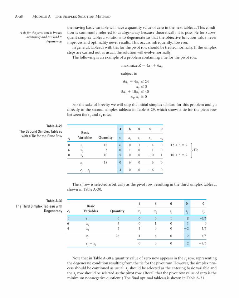
The following is an example of a problem containing a tie for the pivot row.


subject to

6x1 � 4x2 � 24x2 � 3

5x1 � 10x2 � 40x1, x2 � 0

For the sake of brevity we will skip the initial simplex tableau for this problem and godirectly to the second simplex tableau in Table A-29, which shows a tie for the pivot rowbetween the s1 and s3 rows.

The s3 row is selected arbitrarily as the pivot row, resulting in the third simplex tableau,shown in Table A-30.

Note that in Table A-30 a quantity value of zero now appears in the s1 row, representingthe degenerate condition resulting from the tie for the pivot row. However, the simplex pro-cess should be continued as usual: s2 should be selected as the entering basic variable andthe s1 row should be selected as the pivot row. (Recall that the pivot row value of zero is theminimum nonnegative quotient.) The final optimal tableau is shown in Table A-31.

A tie for the pivot row is brokenarbitrarily and can lead to

degeneracy.

Basic4 6 0 0 0

cj Variables Quantity x1 x2 s1 s2 s3

0 s1 12 6 0 1 �4 0 12 ÷ 6 � 2

6 x2 3 0 1 0 1 0 Tie

0 s3 10 5 0 0 �10 1 10 ÷ 5 � 2

zj 18 0 6 0 6 0

cj � zj 4 0 0 �6 0

�

Basic4 6 0 0 0


0 s1 0 0 0 1 8 6/5

6 x2 3 0 1 0 1 0

4 x1 2 1 0 0 �2 1/5

zj 26 4 6 0 �2 4/5

cj � zj 0 0 0 2 �4/5


Basic4 6 0 0 0


0 s2 0 0 0 1/8 1 �3/20

6 x2 3 0 1 �1/8 0 3/20

4 x1 2 1 0 1/4 0 �1/10

zj 26 4 6 1/4 0 1/2

cj � zj 0 0 �1/4 0 �1/2


for a Degenerate Problem

2

20

x1

x2

4 6 8

4

6

8

C

BA

6x1 + 4x2 = 24

5x1 + 10x2 = 40

x2 = 3

Figure A-8

Graph of a degenerate solution

Notice that the optimal solution did not change from the third to the optimal simplextableau. The graphical analysis of this problem shown in Figure A-8 reveals the reason forthis.

Degeneracy occurs in a simplexproblem when a problem

continually loops back to the samesolution or tableau.

Negative Quantity Values

Standard form for simplexsolution requires positive

right-hand-side values.

Notice that in the third tableau (Table A-30) the simplex process went to point B, whereall three constraint lines intersect. This is, in fact, what caused the tie for the pivot row andthe degeneracy. Subsequently, the simplex process stayed at point B in the optimal tableau(Table A-31). The two tableaus represent two different basic feasible solutions correspond-ing to two different sets of model constraint equations.

Occasionally a model constraint is formulated with a negative quantity value on the rightside of the inequality sign—for example,

�6x1 � 2x2 � �30

This is an improper condition for the simplex method, because for the method to work, allquantity values must be positive or zero.

This difficulty can be alleviated by multiplying the inequality by �1, which also changesthe direction of the inequality.

(�1) (�6x1 � 2x2 � �30)6x1 � 2x2 � 30

A negative right-hand-side valueis changed to a positive by multi-

plying the constraint by –1, whichchanges the inequality sign.


The Dual

Now the model constraint is in proper form to be transformed into an equation and solvedby the simplex method.

Multiple optimal solutions are identified by cj � zj (or zj � cj) � 0 for a nonbasic variable.To determine the alternate solution(s), enter the nonbasic variable(s) with a cj � zj valueequal to zero.

An infeasible problem is identified in the simplex procedure when an optimal solution isachieved (i.e., when all cj � zj � 0) and one or more of the basic variables are artificial.

An unbounded problem is identified in the simplex procedure when it is not possible toselect a pivot row—that is, when the values obtained by dividing the quantity values by thecorresponding pivot column values are negative or undefined.

Summary of SimplexIrregularities

The original linear programmingmodel is called the primal, andthe alternative form is the dual.

Every linear programming model has two forms: the primal and the dual. The originalform of a linear programming model is called the primal. All the examples in this moduleare primal models. The dual is an alternative model form derived completely from the pri-mal. The dual is useful because it provides the decision maker with an alternative way oflooking at a problem. Whereas the primal gives solution results in terms of the amount ofprofit gained from producing products, the dual provides information on the value of theconstrained resources in achieving that profit.

The following example will demonstrate how the dual form of a model is derived andwhat it means. The Hickory Furniture Company produces tables and chairs on a dailybasis. Each table produced results in $160 in profit; each chair results in $200 in profit. Theproduction of tables and chairs is dependent on the availability of limited resources—labor, wood, and storage space. The resource requirements for the production of tables andchairs and the total resources available are as follows.

Resource Requirements

Resource Table Chair Total Available per Day

Labor (hr) 2 4 40

Wood (bd ft) 18 18 216

Storage (ft2) 24 12 240

The company wants to know the number of tables and chairs to produce per day tomaximize profit. The model for this problem is formulated as follows.


subject to

2x1 � 4x2 � 40 hr of labor18x1 � 18x2 � 216 bd ft of wood24x1 � 12x2 � 240 ft2 of storage space

x1, x2 � 0

The dual solution variablesprovide the value of the resources,

that is, shadow prices.

The Dual A-31

The dual is formulated entirelyfrom the primal.

A primal maximization modelwith � constraints converts to

a dual minimization modelwith � constraints, and vice versa.

where

x1 � number of tables producedx2 � number of chairs produced

This model represents the primal form. For a primal maximization model, the dual form isa minimization model. The dual form of this example model is

minimize Z � 40y1 � 216y2 � 240y3

subject to

2y1 � 18y2 � 24y3 � 1604y1 � 18y2 � 12y3 � 200

y1, y2, y3 � 0

The specific relationships between the primal and the dual demonstrated in thisexample are as follows.

1. The dual variables, y1, y2, and y3, correspond to the model constraints in the primal.For every constraint in the primal there will be a variable in the dual. For example,in this case the primal has three constraints; therefore, the dual has three decisionvariables.

2. The quantity values on the right-hand side of the primal inequality constraints arethe objective function coefficients in the dual. The constraint quantity values in theprimal, 40, 216, and 240, form the dual objective function: Z � 40y1 � 216y2 �240y3.

3. The model constraint coefficients in the primal are the decision variable coefficientsin the dual. For example, the labor constraint in the primal has the coefficients 2 and4. These values are the y1 variable coefficients in the model constraints of the dual:2y1 and 4y1.

4. The objective function coefficients in the primal, 160 and 200, represent the modelconstraint requirements (quantity values on the right-hand side of the constraint) inthe dual.

5. Whereas the maximization primal model has � constraints, the minimization dualmodel has � constraints.

The primal – dual relationships can be observed by comparing the two model forms shownin Figure A-9.

Now that we have developed the dual form of the model, the next step is determiningwhat the dual means. In other words, what do the decision variables y1, y2, and y3 mean,what do the � model constraints mean, and what is being minimized in the dual objectivefunction?

The dual model can be interpreted by observing the simplex solution to the primal form ofthe model. The simplex solution to the primal model is shown in Table A-32.

Interpreting this primal solution, we have

x1 � 4 tablesx2 � 8 chairss3 � 48 ft2 of storage spaceZ � $2,240 profit

Interpreting the Dual Model


Basic 160 200 0 0 0


200 x2 8 0 1 1�2 �1�18 0

160 x1 4 1 0 �1�2 1�9 0

0 s3 48 0 0 6 �2 1

zj 2,240 160 200 20 20�3 0

cj� zj 0 0 �20 �20�3 0

Table A-32The Optimal Simplex Solution

for the Primal Model

cj qi

160

200

160 200 40 216 240

40

216

240

4

18

12

2

18

24

2y1 + 18y2 + 24y3

4y1 + 18y2 + 12y3

x2 �

x2 �

x2 �

y1, y2, y3 0�

subject to:subject to:

Primal Dual

minimize Zd = y1 + y2 + y3maximize Zp = x1 + x2

x1 +

x1 +

x1 +

�

�

x1, x2 0�

Figure A-9

The primal – dual relationships

This optimal primal tableau also contains information about the dual. In the cj � zj row ofTable A-32, the negative values of �20 and �20/3 under the s1 and s2 columns indicate thatif one unit of either s1 or s2 were entered into the solution, profit would decrease by $20 or$6.67 (i.e., 20/3), respectively.

Recall that s1 represents unused labor and s2 represents unused wood. In the presentsolution s1 and s2 are not basic variables, so they both equal zero. This means that all of thematerial and labor are being used to make tables and chairs, and there are no excess (slack)labor hours or board feet of material left over. Thus, if we enter s1 or s2 into the solution,then s1 or s2 no longer equals zero, we would be decreasing the use of labor or wood. If, forexample, one unit of s1 is entered into the solution, then one unit of labor previously usedis not used, and profit is reduced by $20.

Let us assume that one unit of s1 has been entered into the solution so that we have onehour of unused labor (s1 � 1). Now let us remove this unused hour of labor from the solu-tion so that all labor is again being used. We previously noted that profit was decreased by$20 by entering one hour of unused labor; thus, it can be expected that if we take this hourback (and use it again), profit will be increased by $20. This is analogous to saying that if wecould get one more hour of labor, we could increase profit by $20. Therefore, if we couldpurchase one hour of labor, we would be willing to pay up to $20 for it because that is theamount by which it would increase profit.

The negative cj � zj row values of $20 and $6.67 are the marginal values of labor (s1) andwood (s2), respectively. These dual values are also often referred to as shadow prices, sincethey reflect the maximum “price” one would be willing to pay to obtain one more unit ofthe resource.

What happened to the third resource, storage space? The answer can be seen in Table A-32. Notice that the cj � zj row value for s3 (which represents unused storage space) iszero. This means that storage space has a marginal value of zero; that is, we would not bewilling to pay anything for an extra foot of storage space.

The reason more storage space has no marginal value is because storage space was nota limitation in the production of tables and chairs. Table A-32 shows that 48 square feet ofstorage space were left unused (i.e., s3 � 48) after the 4 tables and 8 chairs were produced.Since the company already has 48 square feet of storage space left over, an extra square footwould have no additional value; the company cannot even use all of the storage space it hasavailable.

We need to consider one additional aspect of these marginal values. In our discussionof the marginal value of these resources, we have indicated that the marginal value (orshadow price) is the maximum amount that would be paid for additional resources. Themarginal value of $60 for one hour of labor is not necessarily what the HickoryFurniture Company would pay for an hour of labor. This depends on how the objectivefunction is defined. In this example we are assuming that all of the resources available,40 hours of labor, 216 board feet of wood, and 240 square feet of storage space, arealready paid for. Even if the company does not use all the resources, it still must pay forthem. They are sunk costs. In other words, the cost of any additional resources securedare included in the objective function coefficients. As such, the profit values in the objec-tive function for each product are unaffected by how much of a resource is actually used;the profit is independent of the resources used. If the cost of the resources is notincluded in the profit function, then securing additional resources would reduce themarginal value.

Continuing our analysis, we note that the profit in the primal model was shown to be$2,240. For the furniture company, the value of the resources used to produce tables andchairs must be in terms of this profit. In other words, the value of the labor and woodresources is determined by their contribution toward the $2,240 profit. Thus, if the com-pany wanted to assign a value to the resources it used, it could not assign an amount greaterthan the profit earned by the resources. Conversely, using the same logic, the total value ofthe resources must also be at least as much as the profit they earn. Thus, the value of all theresources must exactly equal the profit earned by the optimal solution.

Now let us look again at the dual form of the model.

The Dual A-33

John Von Neumann, the famous Hungarian mathematician, iscredited with many contributions in science and mathematics,including crucial work on the development of the atomicbomb during World War II and the development of the com-puter following the war. In 1947 George Dantzig visited Von

Neumann at the Institute for Advanced Study at Princeton anddescribed the linear programming technique to him. VonNeumann grasped the technique immediately, because he hadbeen working on similar concepts himself, and went on toexplain duality to Dantzig for the first time.

for John Von NeumannTime Out

The cj�zj values for slack variablesare the marginal values of the con-

straint resources, i.e., shadow prices.

If a resource is not completelyused, i.e., there is slack, its

marginal value is zero.

The shadow price is the maxi-mum amount that should be paid

for one additional unit of aresource.

The total marginal value of theresources equals the optimal profit.


Sensitivity Analysis

minimize Zd � 40y1 � 16y2 � 240y3

subject to

2y1 � 18y2 � 24y3 � 1604y1 � 18y2 � 12y3 � 200

y1, y2, y3, � 0

Given the previous discussion on the value of the model resources, we can now definethe decision variables of the dual, y1, y2, and y3, to represent the marginal values of theresources:

y1 � marginal value of 1 hr of labor � $20y2 � marginal value of 1 bd ft of wood � $6.67y3 � marginal value of 1 ft2 of storage space � $0

The importance of the dual to the decision maker lies in the information it provides aboutthe model resources. Often the manager is less concerned about profit than about the use ofresources because the manager often has more control over the use of resources than overthe accumulation of profits. The dual solution informs the manager of the value of theresources, which is important in deciding whether or not to secure more resources and howmuch to pay for these additional resources.

If the manager secures more resources, the next question is “How does this affect theoriginal solution?” The feasible solution area is determined by the values forming themodel constraints, and if those values are changed, it is possible for the feasible solutionarea to change. The effect on the solution of changes to the model is the subject of sensitiv-ity analysis, the next topic to be presented here.

The dual variables equal themarginal value of the resources,

the shadow prices.

Use of the Dual

The dual provides the decisionmaker with a basis for deciding

how much to pay for moreresources.

In this section we will show how sensitivity ranges are mathematically determined usingthe simplex method. While this is not as efficient or quick as using the computer, closeexamination of the simplex method for performing sensitivity analysis can provide a morethorough understanding of the topic.

To demonstrate sensitivity analysis for the coefficients in the objective function, we will usethe Hickory Furniture Company example developed in the previous section. The model forthis example was formulated as


subject to


x1, x2 � 0

where

x1 � number of tables producedx2 � number of chairs produced

Changes in ObjectiveFunction Coefficients

Sensitivity Analysis A-35

Figure A-10

A change in c1

5

50

x1

x2

10 15 20

10

15

20

AB

CD

c1 = 250

c1 = 160

Basic 160 200 0 0 0


200 x2 8 0 1 1�2 �1�18 0

160 x1 4 1 0 �1�2 1�9 0

0 s3 48 0 0 6 �2 1

zj 2,240 160 200 20 20�3 0

cj � zj 0 0 �20 �20�3 0


The coefficients in the objective function will be represented symbolically as cj (the samenotation used in the simplex tableau). Thus, c1 � 160 and c2 � 200. Now, let us considera change in one of the cj values by an amount �. For example, let us change c1 � 160 by� � 90. In other words, we are changing c1 from $160 to $250. The effect of this change onthe solution of this model is shown graphically in Figure A-10.

Originally, the solution to this problem was located at point B in Figure A-10, wherex1 � 4 and x2 � 8. However, increasing c1 from $160 to $250 shifts the slope of the objec-tive function so that point C (x1 � 8, x2 � 4) becomes the optimal solution. This demon-strates that a change in one of the coefficients of the objective function can change the opti-mal solution. Therefore, sensitivity analysis is performed to determine the range overwhich cj can be changed without altering the optimal solution.

The range of cj that will maintain the optimal solution can be determined directly fromthe optimal simplex tableau. The optimal simplex tableau for our furniture companyexample is shown in Table A-33.

The sensitivity range for a cj valueis the range of values over whichthe current optimal solution will

remain optimal.

First, consider a � change for c1. This will change the c1 value from c1 � 160 toc1 � 160 � �, as shown in Table A-34. Notice that when c1 is changed to 160 � �, the newvalue is included not only in the top cj row but also in the left-hand cj column. This isbecause x1 is a basic solution variable. Since 160 � � is in the left-hand column, it becomes

� is added to cj in the optimal

simplex tableau.


Basic160 � � 200 0 0 0


200 x2 8 0 1 1�2 �1�18 0

160 � � x1 4 1 0 �1�2 1�9 0

0 s3 48 0 0 6 �2 1

zj 2,240 � 4� 160 � � 200 20 � ��2 20�3 � ��9 0

cj � zj 0 0 �20 � ��2 �20�3 � ��9 0


with c1 � 160 + �

a multiple of the column values when the new zj row values and the subsequent cj � zj rowvalues, also shown in Table A-34, are computed.

The solution shown in Table A-34 will remain optimal as long as the cj � zj row valuesremain negative. (If cj � zj becomes positive, the product mix will change, and if it becomeszero, there will be an alternative solution.) Thus, for the solution to remain optimal,

�20 � ��2 � 0

and

�20�3 � ��9 � 0

Both of these inequalities must be solved for �.

�20 � ��2 � 0��2 � 20

� � 40

and

�20/3 � ��9 � 0��9 � 20�3

�� 60� � �60

Thus, � � 40 and � � �60. Now recall that c1 � 160 � �; therefore, � � c1 � 160.Substituting the amount c1�160 for � in these inequalities,

� � 40c1 � 160 � 40

c1 � 200

and

� � �60c1 � 160 � �60

c1 � 100

Therefore, the range of values for c1 over which the solution basis will remain optimal(although the value of the objective function may change) is

100 � c1 � 200

Next, consider a � change in c2 so that c2 � 200 � �. The effect of this change in thefinal simplex tableau is shown in Table A-35.

For the solution to remain optimalall values in the cj � zj row must

be � 0.


Basic160 200 � � 0 0 0


200 � � x2 8 0 1 1�2 �1�18 0

160 x1 4 1 0 �1�2 1�9 0

0 s3 48 0 0 6 �2 1

zj 2,240 � 8� 160 200 � � 20 � ��2 20�3 � ��18 0

cj � zj 0 0 �20 � ��2 �20�3 � ��18 0


with c2 � 200 � �

As before, the solution shown in Table A-35 will remain optimal as long as the cj � zjrow values remain negative or zero. Thus, for the solution to remain optimal, we must have

�20 � ��2 � 0

and

�20�3 � ��18 � 0

Solving these inequalities for � gives

�20 ��2 � 0��2 � 20

� � �40

and

�20�3 � ��18 � 0��18 � 20�3

� � 120

Thus, � � �40 and � � 120. Since c2 � 200 � �, we have � � c2 � 200. Substitutingthis value for � in the inequalities yields

� � �40c2 �200 � �40

c2 � 160

and

� � 120c2 �200 � 120

c2 � 320

Therefore, the range of values for c2 over which the solution will remain optimal is

160 � c2 � 320

The ranges for both objective function coefficients are as follows.

100 � c1 � 200160 � c2 � 320

However, these ranges reflect a possible change in either c1 or c2, not simultaneouschanges in both c1 and c2. Both of the objective function coefficients in this example werefor basic solution variables. Determining the cj sensitivity range for a decision variable thatis not basic is much simpler. Because it is not in the basic variable column, the � change


Figure A-11

A � change in q2

5

50

x1

x2

10 15 20

10

15

20

AB

CD

B'C'

Original optimal solution

New optimal solutionwith change in q2

does not become a multiple of the zj row. Thus, the � change will show up in only one col-umn in the cj � zj row.

To demonstrate the effect of a change in the quantity values of the model constraints, wewill again use the Hickory Furniture Company example.


subject to


x1, x2 � 0

The quantity values 40, 216, and 240 will be represented symbolically as qi. Thus, q1 � 40,q2 � 216, and q3 � 240. Now consider a � change in q2. For example, let us change q2 � 216by � � 18. In other words, q2 is changed from 216 board feet to 234 board feet. The effectof this change is shown graphically in Figure A-11.

In Figure A-11 a change in q2 is shown to have the effect of changing the feasible solutionarea from 0ABCD to 0AB C D. Originally, the optimal solution point was B; however, thechange in q2 causes B to be the new optimal solution point. At point B the optimal solution is

x1 � 4x2 � 8s3 � 48

s1 and s2 � 0Z � $2,240

At point B the new optimal solution is

x1 � 6x2 � 7

Changes in ConstraintQuantity Values



s3 � 12s1 and s2 � 0

Z � $2,360

Thus, a change in a qi value can change the values of the optimal solution. At some point anincrease or decrease in qi will change the variables in the optimal solution mix, includingthe slack variables. For example, if q2 increases to 240 board feet, then the optimal solutionpoint will be at

x1 � 6.67x2 � 6.67s3 � 0

s1 and s2 � 0Z � $2,400

Notice that s3 has left the solution; thus, the optimal solution mix has changed. At thispoint, where q2 � 240, which is the upper limit of the sensitivity range for q2, the shadowprice will also change. Therefore, the purpose of sensitivity analysis is to determine therange for qi over which the optimal variable mix will remain the same and the shadow pricewill remain the same.

As in the case of the cj values, the range for qi can be determined directly from the opti-mal simplex tableau. As an example, consider a � increase in the number of labor hours.The model constraints become

2x1 � 4x2 � 40 � 1�18x1 � 18x2 � 216 � 0�24x1 � 12x2 � 240 � 0�

Notice in the initial simplex tableau for our example (Table A-36) that the changes inthe quantity column are the same as the coefficients in the s1 column.

The sensitivity range for a qi,value is the range of values over

which the right-hand-side valuescan vary without changing the

solution variable mix, includingslack variables and the shadow

prices.

This duplication will carry through each subsequent tableau, so the s1 column valueswill duplicate the � changes in the quantity column in the final tableau (Table A-37).

In effect, the � changes form a separate column identical to the s1 column. Therefore, todetermine the � change, we need only observe the slack (si) column corresponding to themodel constraint quantity (qi) being changed.

Recall that a requirement of the simplex method is that the quantity values not be nega-tive. If any qi value becomes negative, the current solution will no longer be feasible anda new variable will enter the solution. Thus, the inequalities

A � in a qi value is duplicated inthe si column in the final tableau.

Basic160 200 0 0 0


0 1 40 � 1� 2 4 1 0 0

0 s2 216 � 0� 18 18 0 1 0

0 s3 240 � 0� 24 12 0 0 1

zj 0 0 0 0 0 0

cj � zj 160 200 0 0 0


Basic160 200 0 0 0


200 x2 8 � �/2 0 1 1/2 �1/18 0

160 x1 4 � �/2 1 0 �1/2 1/9 0

0 s3 48 � 6� 0 0 6 �2 1

zj 2,240 � 20� 160 200 20 20/3 0

cj � zj 0 0 �20 �20/3 0

Table A-37The Final Simplex Tableau

8 � ��2 � 04 � ��2 � 048 � 6� � 0

are solved for �:

8 � ��2 � 0��2 � �8

� � �16

and

4 � ��2 � 0��2 � �4

� � 8

and

48 � 6� � 06� � �48� � �8

Since

q1 � 40 � �

then

� � q1 �40

These values are substituted into the inequalities � � �16, � � 8, and � � �8 as follows.

� � �16q1 �40 � �16

q1 � 24� � 8

q1 �40 � 8q1 � 48� � �8

q1 �40 � �8q1 � 32

Summarizing these inequalities, we have

24 � 32 � q1 � 48


The value of 24 can be eliminated, since q1 must be greater than 32; thus,

32 � q1 � 48

As long as q1 remains in this range, the present basic solution variables will remain thesame and feasible. However, the quantity values of those basic variables may change. Inother words, although the variables in the basis remain the same, their values can change.

To determine the range for q2 (where q2 � 216 � �), the s2 column values are used todevelop the � inequalities.

8 � ��18 � 04 � ��9 � 048 � 2� � 0

The inequalities are solved as follows.

8 � ��18 � 0��18 � �8

� � 144

4 � ��9 � 0��9 � �4

� � �36

48 � 2� � 0�2� � �48

� � 24

Since

q2 � 216 � �

we have

� � q2 � 216

Substituting this value into the inequalities � � 144, � � �36, and � � 24 gives a range ofpossible values for q2:

� � 144q2�216 � 144

q2 � 360

� � �36q2�216 � �36

q2 � 180

� � 24q2�216 � 24

q2 � 240

That is,

180 � q2 � 240 � 360


The value 360 can be eliminated, because q2 cannot exceed 240. Thus, the range overwhich the basic solution variables will remain the same is

180 � q2 � 240

The range for q3 is

192 � q3 � �

The upper limit of means that q3 can increase indefinitely (without limit) withoutchanging the optimal variable solution mix in the shadow price.

Sensitivity analysis of constraint quantity values can be used in conjunction with thedual solution to make decisions regarding model resources. Recall from our analysis of thedual solution of the Hickory Furniture Company example that

y1 � $20, marginal value of labory2 � $6.67, marginal value of woody3 � $0, marginal value of storage space

Because the resource with the greatest marginal value is labor, the manager might desireto secure some additional hours of labor. How many hours should the manager get? Giventhat the range for q1 is 32 � q1 � 48, the manager could secure up to an additional 8 hoursof labor (i.e., 48 total hours) before the solution basis changes and the shadow price alsochanges. If the manager did purchase 8 more hours, the solution values could be found byobserving the quantity values in Table A-37.

x2 � 8 � ��2x1 � 4 � ��2s3 � 48 � 6�

Since � � 8,

x2 � 8 � (8)/2� 12

x1 � 4 � (8)/2� 0

s3 � 48 � 6(8)� 96

Total profit will be increased by $20 for each extra hour of labor.

Z � $2,240 � 20�� 2,240 � 20(8)� 2,240 � 160� $2,400

In this example for the Hickory Furniture Company, we considered only � constraintsin determining the sensitivity ranges for qi values. To compute the qi sensitivity range, weobserved the slack column, si, since a � change in qi was reflected in the si column.However, recall that with a constraint we subtract a surplus variable rather than addinga slack variable to form an equality (in addition to adding an artificial variable). Thus, fora constraint we must consider a �� change in qi in order to use the si (surplus) columnto perform sensitivity analysis. In that case sensitivity analysis would be performed exactly

�

The shadow prices are only validwith the sensitivity range for the

right-hand-side values.

Problems A-43

Problems

as shown in this example, except that the value of qi � � would be used instead of qi � �when computing the sensitivity range for qi.

1. Following is a simplex tableau for a linear programming model.

Basic10 2 6 0 0 0

cj Variables Quantity x1 x2 x3 s1 s2 s3

2 x1 10 0 1 �2 1 �1�2 010 x2 40 1 0 2 0 1�2 0

0 s3 30 0 0 8 �3 3�2 1

zj 420 10 2 16 2 4 0

cj � zj 0 0 �10 �2 �4 0

a. What is the solution given in this tableau?b. Is the solution in this tableau optimal? Why?c. What does x3 equal in this tableau? s2?d. Write out the original objective function for the linear programming model, using only decision

variables.e. How many constraints are in the linear programming model?f. Explain briefly why it would have been difficult to solve this problem graphically.

2. The following is a simplex tableau for a linear programming model.

Basic6 20 12 0 0

cj Variables Quantity x1 x2 x3 s1 s2

6 x1 20 1 1 0 0 012 x3 10 0 1�3 1 0 �1�60 s1 10 0 1�3 0 1 �1�6

zj 240 6 10 12 0 �2

zj � cj 0 �10 0 0 �2

a. Is this a maximization or a minimization problem? Why?b. What is the solution given in this tableau?c. Is the solution given in this tableau optimal? Why?


d. Write out the original objective function for the linear programming model using only decisionvariables.

e. How many constraints are in the linear programming model?f. Were any of the constraints originally equations? Why?g. What is the value of x2 in this tableau?

3. The following is a simplex tableau for a linear programming problem.

Basic60 50 45 50 0 0 0 0

cj Variables Quantity x1 x2 x3 x4 s1 s2 s3 s4

0 s1 20 0 1 0 0 1 0 0 050 x4 15 0 0 0 1 0 1 0 060 x1 12 1 1�2 0 0 0 0 1�10 0

0 s4 45 0 0 8 6 0 �6 0 1

zj 1,470 60 30 0 50 0 50 6 0

cj � zj 0 20 45 0 0 �50 �6 0

a. Is this a maximization or a minimization problem?b. What are the values of the decision variables in this tableau?c. What are the values of the slack variables in this tableau?d. What does the cj � zj value of “20” in the “x2” column mean?e. Is this solution optimal? Why? If the solution is not optimal, determine the optimal solution.

4. The following is a simplex tableau for a linear programming problem.

Basic8 10 4 0 0 0 M M

cj Variables Quantity x1 x2 x3 s1 s2 s3 A1 A2

M A1 30 2�3 0 1 �1 1�6 0 0 010 x2 10 1�3 1 0 0 �1�6 0 1 0M A3 100 0 0 1 0 0 �1 0 1

zj 130M � 100 2M�3 � 10�3 10 2M �M M�6 � 5�3 �M M M

zj � cj 2M�3 � 14�3 0 2M � 4 �M M�6 � 5�3 �M 0 0

a. Is this a maximization or a minimization problem?b. What is the value of x3 in this tableau?c. What does the value “M�6 � 5�3” in the “s2” column of the zj � cj row mean?d. What is the minimum number of additional simplex iterations that this problem must go

through to determine a feasible optimal solution?e. Is this solution optimal? Why? If the solution is not optimal, compute the optimal solution.

Problems A-45

5. Given is the following simplex tableau for a linear programming problem.

Basic4 6 0 0 M


M A1 2 0 1�2 �1 1�2 14 x1 6 1 1�2 0 �1�2 0

zj 24 � 2M 4 M�2 � 2 �M M�2 � 2 M

zj � cj 0 M�2 � 4 �M M�2 � 2 0

a. Is this a maximization or a minimization problem? Why?b. What are the values of the decision variables in this tableau?c. Were any of the constraints in this problem originally equations? Why?d. What is the value of s2 in this tableau?e. Is this solution optimal? Why? If the solution is not optimal, complete the next iteration

(tableau) and indicate if it is optimal.

6. Following is a simplex tableau for a linear programming problem.

Basic10 5 0 0 �M


10 x1 5 1 1�2 �1�2 0 0�M A2 4 0 1 0 0 1

0 s2 15 0 7�2 1�2 1 0

zj �4M � 50 10 �M � 5 �5 0 �M

cj � zj 0 M 5 0 0

a. Is this a maximization or a minimization problem? Why?b. What is the value of x2 in this tableau?c. Does the fact that x1 has a cj � zj value equal to “0” in this tableau mean that multiple optimal

solutions exist? Why?d. What does the cj � zj value for the s1 column mean?e. Is this solution optimal? Why? If not, solve this problem and indicate if multiple optimal solu-

tions exist.

7. The Munchies Cereal Company makes a cereal from several ingredients. Two of the ingredients,oats and rice, provide vitamins A and B. The company wants to know how many ounces of oats andrice it should include in each box of cereal to meet the minimum requirements of 48 milligrams ofvitamin A and 12 milligrams of vitamin B while minimizing cost. An ounce of oats contributes8 milligrams of vitamin A and 1 milligram of vitamin B, whereas an ounce of rice contributes


6 milligrams of vitamin A and 2 milligrams of vitamin B. An ounce of oats costs $0.05, and anounce of rice costs $0.03. Formulate a linear programming model for this problem and solve usingthe simplex method.

8. A company makes product 1 and product 2 from two resources. The linear programming modelfor determining the amounts of product 1 and 2 to produce (x1 and x2) is

maximize Z � 8x1 � 2x2 (profit, $)

subject to

4x1 � 5x2 � 20 (resource 1, lb)2x1 � 6x2 � 18 (resource 2, lb)

x1, x2 0

Solve this model using the simplex method.

9. A company produces two products that are processed on two assembly lines. Assembly line 1 has100 available hours, and assembly line 2 has 42 available hours. Each product requires 10 hours ofprocessing time on line 1, while on line 2 product 1 requires 7 hours and product 2 requires3 hours. The profit for product 1 is $6 per unit, and the profit for product 2 is $4 per unit.Formulate a linear programming model for this problem and solve using the simplex method.

10. The Pinewood Furniture Company produces chairs and tables from two resources — labor andwood. The company has 80 hours of labor and 36 pounds of wood available each day. Demand forchairs is limited to 6 per day. Each chair requires 8 hours of labor and 2 pounds of wood to pro-duce, while a table requires 10 hours of labor and 6 pounds of wood. The profit derived from eachchair is $400 and from each table, $100. The company wants to determine the number of chairs andtables to produce each day to maximize profit. Formulate a linear programming model for thisproblem and solve using the simplex method.

11. The Crumb and Custard Bakery makes both coffee cakes and Danish in large pans. The main ingre-dients are flour and sugar. There are 25 pounds of flour and 16 pounds of sugar available and thedemand for coffee cakes is 8. Five pounds of flour and 2 pounds of sugar are required to make onepan of coffee cake, and 5 pounds of flour and 4 pounds of sugar are required to make one pan ofDanish. One pan of coffee cake has a profit of $1, and one pan of Danish has a profit of $5.Determine the number of pans of cake and Danish that the bakery must produce each day so thatprofit will be maximized. Formulate a linear programming model for this problem and solve usingthe simplex method.

12. The Kalo Fertilizer Company makes a fertilizer using two chemicals that provide nitrogen, phos-phate, and potassium. A pound of ingredient 1 contributes 10 ounces of nitrogen and 6 ounces ofphosphate, whereas a pound of ingredient 2 contributes 2 ounces of nitrogen, 6 ounces of phos-phate, and 1 ounce of potassium. Ingredient 1 costs $3 per pound, and ingredient 2 costs $5 perpound. The company wants to know how many pounds of each chemical ingredient to put into abag of fertilizer to meet minimum requirements of 20 ounces of nitrogen, 36 ounces of phosphate,and 2 ounces of potassium while minimizing cost. Formulate a linear programming model for thisproblem and solve using the simplex method.

13. Solve the following model using the simplex method.

minimize Z � 0.06x1 � 0.10x2

subject to

Problems A-47

4x1 � 3x2 123x1 � 6x2 125x1 � 2x2 10

x1, x2 0

14. The Copperfield Mining Company owns two mines, both of which produce three grades of ore —high, medium, and low. The company has a contract to supply a smelting company with at least 12tons of high-grade ore, 8 tons of medium-grade ore, and 24 tons of low-grade ore. Each mine pro-duces a certain amount of each type of ore each hour it is in operation. Mine 1 produces 6 tons ofhigh-grade, 2 tons of medium-grade, and 4 tons of low-grade ore per hour. Mine 2 produces 2 tonsof high-grade, 2 tons of medium-grade, and 12 tons of low-grade ore per hour. It costs $200 perhour to mine each ton of ore from mine 1, and it costs $160 per hour to mine a ton of ore frommine 2. The company wants to determine the number of hours it needs to operate each mine sothat contractual obligations can be met at the lowest cost. Formulate a linear programming modelfor this problem and solve using the simplex method.

15. A marketing firm has contracted to do a survey on a political issue for a Spokane television station.The firm conducts interviews during the day and at night, by telephone and in person. Each houran interviewer works at each type of interview results in an average number of interviews. In orderto have a representative survey, the firm has determined that there must be at least 400 day inter-views, 100 personal interviews, and 1,200 interviews overall. The company has developed thefollowing linear programming model to determine the number of hours of telephone interviewsduring the day (x1), telephone interviews at night (x2), personal interviews during the day (x3), andpersonal interviews at night (x4) that should be conducted to minimize cost.

minimize Z � 2x1 � 3x2 � 5x3 � 7x4 (cost, $)

subject to

10x1 � 4x3 400 (day interviews)4x3 � 5x4 100 (personal interviews)

x1 � x2 � x3 � x4 1,200 (total interviews)x1, x2, x3, x4 0


16. A jewelry store makes both necklaces and bracelets from gold and platinum. The store has devel-oped the following linear programming model for determining the number of necklaces andbracelets (x1 and x2) that it needs to make to maximize profit.


subject to

3x1 � 2x2 � 18 (gold, oz)2x1 � 4x2 � 20 (platinum, oz)

x2 � 4 (demand, bracelets)x1, x2 0


17. A sporting goods company makes baseballs and softballs on a daily basis from leather and yarn.The company has developed the following linear programming model for determining the numberof baseballs and softballs to produce (x1 and x2) to maximize profits:



subject to

0.3x1 � 0.5x2 � 150 (leather, ft2)10x1 � 4x2 � 2,000 (yarn, yd)

x1, x2 0


18. A clothing shop makes suits and blazers. Three main resources are used: material, rack space, andlabor. The shop has developed this linear programming model for determining the number of suitsand blazers to make (x1 and x2) to maximize profits:


subject to

10x1 � 4x2 � 160 (material, yd2)x1 � x2 � 20 (rack space)

10x1 � 20x2 � (labor, hr)x1, x2 0


19. Solve the following linear programming model using the simplex method.

maximize Z � 100x1 � 20x2 � 60x3

subject to

3x1 � 5x2 � 602x1 � 2x2 � 2x3 � 100

x3 � 40x1, x2, x3 0

20. The following is a simplex tableau for a linear programming model.

Basic1 2 �1 0 0 0


2 x2 10 0 1 1�4 1�4 0 00 s2 20 0 0 �3�4 3�4 1 �1�21 x1 10 1 0 1 �1�2 0 1�2

zj 30 1 2 3�2 0 0 1�2

cj � zj 0 0 �5�2 0 0 �1�2

a. Is this a maximization or a minimization problem? Why?b. What is the solution given in this tableau?c. Write out the original objective function for the linear programming model, using only decision

variables.d. How many constraints are in the linear programming model?e. Were any of the constraints originally equations? Why?f. What does s1 equal in this tableau?

Problems A-49

g. This solution is optimal. Are there multiple optimal solutions? Why?h. If there are multiple optimal solutions, identify the alternate solutions.

21. A wood products firm in Oregon plants three types of trees — white pines, spruce, and ponderosapines — to produce pulp for paper products and wood for lumber. The company wants to plantenough acres of each type of tree to produce at least 27 tons of pulp and 30 tons of lumber. Thecompany has developed the following linear programming model to determine the number ofacres of white pines (x1), spruce (x2), and ponderosa pines (x3) to plant to minimize cost.

minimize Z � 120x1 � 40x2 � 240x3 (cost, $)

subject to

4x1 � x2 � 3x3 27 (pulp, tons)2x1 � 6x2 � 3x3 30 (lumber, tons)

x1, x2, x3 0


22. A baby products firm produces a strained baby food containing liver and milk, each of which con-tribute protein and iron to the baby food. Each jar of baby food must have 36 milligrams of proteinand 50 milligrams of iron. The company has developed the following linear programming model todetermine the number of ounces of liver (x1) and milk (x2) to include in each jar of baby food tomeet the requirements for protein and iron at the minimum cost.

minimize Z � 0.05x1 � 0.10x2 (cost, $)

subject to

6x1 � 2x2 36 (protein, mg)5x1 � 5x2 50 (iron, mg)

x1, x2 0


23. Solve the linear programming model in problem 22 graphically, and identify the points on thegraph that correspond to each simplex tableau.

24. The Cookie Monster Store at South Acres Mall makes three types of cookies — chocolate chip,pecan chip, and pecan sandies. Three primary ingredients are chocolate chips, pecans, and sugar.The store has 120 pounds of chocolate chips, 40 pounds of pecans, and 300 pounds of sugar. Thefollowing linear programming model has been developed for determining the number of batchesof chocolate chip cookies (x1), pecan chip cookies (x2), and pecan sandies (x3) to make to maximizeprofit.

maximize Z � 10x1 � 12x2 � 7x3 (profit, $)

subject to

20x1 � 15x2 � 10x3 � 300 (sugar, lb)10x1 � 5x2 � 120 (chocolate chips, lb)

x1 � 2x3 � 40 (pecans, lb)x1, x2, x3 0



25. The Eastern Iron and Steel Company makes nails, bolts, and washers from leftover steel and coatsthem with zinc. The company has 24 tons of steel and 30 tons of zinc. The following linear pro-gramming model has been developed for determining the number of batches of nails (x1), bolts(x2), and washers (x3) to produce to maximize profit.

maximize Z � 6x1 � 2x2 � 12x3 (profit, $1,000s)

subject to

4x1 � x2 � 3x3 � 24 (steel, tons)2x1 � 6x2 � 3x3 � 30 (zinc, tons)

x1, x2, x3 0



maximize Z � 100x1 � 75x2 � 90x3 � 95x4

subject to

3x1 � 2x2 � 404x3 � x4 � 25

200x1 � 250x3 � 2,000100x1 � 200x4 � 2,200

x1, x2, x3, x4 0


minimize Z � 20x1 � 16x2

subject to

3x1 � x2 6x1 � x2 4

2x1 � 6x2 12x1, x2 0

28. Solve the linear programming model in problem 27 graphically, and identify the points on thegraph that correspond to each simplex tableau.

29. Transform the following linear programming model into proper form for solution by the simplexmethod.

minimize Z � 8x1 � 2x2 � 7x3

subject to

2x1 � 6x2 � x3 � 303x2 � 4x3 60

4x1 � x2 � 2x3 � 50x1 � 2x2 20x1, x2, x3 0

30. Transform the following linear programming model into proper form for solution by the simplexmethod.

Problems A-51

minimize Z � 40x1 � 55x2 � 30x3

subject to

x1 � 2x2 � 3x3 � 602x1 � x2 � x3 � 40x1 � 3x2 � x3 50

5x2 � 3x3 100x1, x2, x3 0

31. A manufacturing firm produces two products using labor and material. The company has acontract to produce 5 of product 1 and 12 of product 2. The company has developed the followinglinear programming model to determine the number of units of product 1 (x1) and product 2 (x2)to produce to maximize profit.


subject to

x1 � 2x2 � 30 (material, lb)4x1 � 4x2 � 72 (labor, hr)

x1 5 (contract, product 1)x2 12 (contract, product 2)

x1, x2 0


32. A custom tailor makes pants and jackets from imported Irish wool cloth. To get any cloth at all, thetailor must purchase at least 25 square feet each week. Each pair of pants and each jacket requires5 square feet of material. The tailor has 16 hours available each week to make pants and jackets. Thedemand for pants is never more than 5 pairs per week. The tailor has developed the following lin-ear programming model to determine the number of pants (x1) and jackets (x2) to make each weekto maximize profit.

maximize Z � x1 � 5x2 (profit, $100s)

subject to

5x1 � 5x2 25 (wool, ft2)2x1 � 4x2 � 16 (labor, hr)

x1 � 5 (demand, pants)x1, x2 0


33. A sawmill in Tennessee produces cherry and oak boards for a large furniture manufacturer. Eachmonth the sawmill must deliver at least 5 tons of wood to the manufacturer. It takes the sawmill3 days to produce a ton of cherry and 2 days to produce a ton of oak, and the sawmill can allocate18 days out of a month for this contract. The sawmill can get enough cherry to make 4 tons ofwood and enough oak to make 7 tons of wood. The sawmill owner has developed the following lin-ear programming model to determine the number of tons of cherry (x1) and oak (x2) to produce tominimize cost.


minimize Z � 3x1 � 6x2 (cost, $)

subject to

3x1 � 2x2 � 18 (production time, days)x1 � x2 5 (contract, tons)

x1 � 4 (cherry, tons)x2 � 7 (oak, tons)

x1, x2 0




subject to

2x1 � x2 10x2 � 4

x1 � 4x2 � 20x1, x2 0

35. Solve the following linear programming problem using the simplex method.

maximize Z � x1 � 2x2 � x3

subject to

4x2 � x3 � 40x1 � x2 � 20

2x1 � 4x2 � 3x3 � 60x1, x2, x3 0

36. Solve the following linear programming problem using the simplex method.

maximize Z � x1 � 2x2 � 2x3

subject to

x1 � x2 � 2x3 � 122x1 � x2 � 5x3 � 20

x1 � x2 � x3 8x1, x2, x3 0

37. A farmer has a 40-acre farm in Georgia. The farmer is trying to determine how many acres of corn,peanuts, and cotton to plant. Each crop requires labor, fertilizer, and insecticide. The farmer hasdeveloped the following linear programming model to determine the number of acres of corn (x1),peanuts (x2), and cotton (x3) to plant to maximize profit.


subject to

2x1 � 3x2 � 2x3 � 120 (labor, hr)4x1 � 3x2 � x3 � 160 (fertilizer, tons)

Problems A-53

3x1 � 2x2 � 4x3 � 100 (insecticide, tons)x1 � x2 � x3 � 40 (acres)

x1, x2, x3 0


38. Solve the following linear programming model (a) graphically and (b) using the simplex method.


subject to

x1 � x2 � 1x1 � x2 2

x1, x2 0

39. Solve the following linear programming model (a) graphically and (b) using the simplex method.

maximize Z � x1 � x2

subject to

x1 � x2 �1�x1 � 2x2 � 4

x1, x2 0


maximize Z � 7x1 � 5x2 � 5x3

subject to

x1 � x2 � x3 � 252x1 � x2 � x3 � 40

x1 � x2 � 25x3 � 6

x1, x2, x3 0


minimize Z � 15x1 � 25x2

subject to

3x1 � 4x2 122x1 � x2 6

3x1 � 2x2 � 9x1, x2 0

42. The Old English Metal Crafters Company makes brass trays and buckets. The number of trays (x1)and buckets (x2) that can be produced daily is constrained by the availability of brass and labor, asreflected in the following linear programming model.



subject to

x1 � 4x2 � 90 (brass, lb)2x1 � 2x2 � 60 (labor, hr)

x1, x2 0

The final optimal simplex tableau for this model is as follows.

Basic6 10 0 0


10 x2 20 0 1 1�3 �1�66 x1 10 1 0 �1�3 2�3

zj 260 6 10 4�3 7�3

cj � zj 0 0 �4�3 �7�3

a. Formulate the dual of this model.b. Define the dual variables and indicate their value.c. Determine the optimal ranges for c1 and c2.d. Determine the feasible ranges for q1 (pounds of brass) and q2 (labor hours).e. What is the maximum price the company would be willing to pay for additional labor hours,

and how many hours could be purchased at that price?

43. The Southwest Foods Company produces two brands of chili — Razorback and Longhorn — fromseveral ingredients, including chili beans and ground beef. The number of 100-gallon batches ofRazorback chili (x1) and Longhorn chili (x2) that can be produced daily is constrained by the avail-ability of chili beans and ground beef, as shown in the following linear programming model.


subject to

10x1 � 50x2 � 500 (chili beans, lb)34x1 � 20x2 � 800 (ground beef, lb)

x1, x2 0


Basic200 300 0 0


300 x2 6 0 1 17�750 �1�150200 x1 20 1 0 �1�75 1�30

zj 5,800 200 300 310�75 70�15

cj � zj 0 0 �310�75 �70�15

Problems A-55

a. Formulate the dual of this model and indicate what the dual variables equal.b. What profit for Razorback chili will result in no Longhorn chili being produced? What will the

new optimal solution values be?c. Determine what the effect will be of changing the amount of beans in Razorback chili from

10 pounds per batch to 15 pounds per batch.d. Determine the optimal ranges for c1 and c2.e. Determine the feasible ranges for q1 (pounds of beans) and q2 (pounds of ground beef).f. What is the maximum price the company would be willing to pay for additional pounds of chili

beans, and how many pounds could be purchased at that price?g. If the company could secure an additional 100 pounds of only one of the ingredients, beans or

ground beef, which should it be?h. If the company changed the selling price of Longhorn chili so that the profit was $400 instead of

$300, would the optimal solution be affected?

44. The Agrimaster Company produces two kinds of fertilizer spreaders — regular and cyclone. Eachspreader must undergo two production processes. Letting x1 � the number of regular spreadersproduced and x2 � the number of cyclone spreaders produced, the problem can be formulated asfollows.


subject to

12x1 � 4x2 � 60 (process 1, production hr)4x1 � 8x2 � 40 (process 2, production hr)

x1, x2 0

The final optimal simplex tableau for this problem is as follows.

Basic9 7 0 0


9 x1 4 1 0 1�10 �1�207 x2 3 0 1 �1�20 3�20

zj 57 9 7 11�20 12�20

cj � zj 0 0 �11�20 �12�20

a. Formulate the dual for this problem.b. Define the dual variables and indicate their values.c. Determine the optimal ranges for c1 and c2.d. Determine the feasible ranges for q1 and q2 (production hours for processes 1 and 2, respect-

ively).e. What is the maximum price the Agrimaster Company would be willing to pay for addi-

tional hours of process 1 production time, and how many hours could be purchased atthat price?


45. The Stratford House Furniture Company makes two kinds of tables — end tables (x1) and coffeetables (x2). The manufacturer is restricted by material and labor constraints, as shown in thefollowing linear programming formulation.


subject to

2x1 � 5x2 � 180 (labor, hr)3x1 � 3x2 � 135 (wood, bd ft)

x1, x2 0

The final optimal simplex tableau for this problem is as follows.

Basic200 300 0 0


300 x2 30 0 1 1�3 �2�9200 x1 15 1 0 �1�3 5�9

zj 12,000 200 300 100�3 400�9

cj � zj 0 0 �100�3 �400�9

a. Formulate the dual for this problem.b. Define the dual variables and indicate their values.c. What profit for coffee tables will result in no end tables being produced, and what will the new

optimal solution values be?d. What will be the effect on the optimal solution if the available wood is increased from 135 to

165 board feet?e. Determine the optimal ranges for c1 and c2.f. Determine the feasible ranges for q1 (labor hours) and q2 (board feet of wood).g. What is the maximum price the Stratford House Furniture Company would be willing to pay

for additional wood, and how many board feet of wood could be purchased at that price?h. If the furniture company wanted to secure additional units of only one of the resources, labor or

wood, which should it be?

46. A manufacturing firm produces electric motors for washing machines and vacuum cleaners. Thefirm has resource constraints for production time, steel, and wire. The linear programming modelfor determining the number of washing machine motors (x1) and vacuum cleaner motors (x2) toproduce has been formulated as follows.


subject to

2x1 � x2 � 19 (production, hr)x1 � x2 � 14 (steel, lb)

x1 � 2x2 � 20 (wire, ft)x1, x2 0


Problems A-57

Basic70 80 0 0 0


70 x1 6 1 0 2�3 0 �1�30 s2 1 0 0 �1�3 1 �1�3

80 x2 7 0 1 �1�3 0 2�3

zj 980 70 80 20 0 30

cj � zj 0 0 �20 0 �30

a. Formulate the dual for this problem.b. What do the dual variables equal, and what do they mean?c. Determine the optimal ranges for c1 and c2.d. Determine the feasible ranges for q1 (production hours), q2 (pounds of steel), and q3 (feet of

wire).e. Managers at the firm have determined that the firm can purchase a new production machine

that will increase available production time from 19 to 25 hours. Would this change affect theoptimal solution?

47. A manufacturer produces products 1 and 2, for which profits are $9 and $12, respectively. Eachproduct must undergo two production processes that have labor constraints. There are alsomaterial constraints and storage limitations. The linear programming model for determiningthe number of product 1 to produce (x1) and the number of product 2 to product (x2) is given asfollows.


subject to

4x1 � 8x2 � 64 (process 1, labor hr)5x1 � 5x2 � 50 (process 2, labor hr)

15x1 � 8x2 � 120 (material, lb)x1 � 7 (storage space, ft2)x2 � 7 (storage space, ft2)

x1, x2 0


Basic9 12 0 0 0 0 0

cj Variables Quantity x1 x2 s1 s2 s3 s4 s5

9 x1 4 1 0 �1�4 2�5 0 0 00 s5 1 0 0 �1�4 1�5 0 0 10 s3 12 0 0 7�4 �22�5 1 0 00 s4 3 0 0 1�4 �2�5 0 1 0

12 x2 6 0 1 1�4 �1�5 0 0 0

zj 108 9 12 3�4 6�5 0 0 0

cj � zj 0 0 �3�4 �6�5 0 0 0


a. Formulate the dual for this problem.b. What do the dual variables equal, and what does this dual solution mean?c. Determine the optimal ranges for c1 and c2.d. Determine the range for q1 (process 1, labor hr).e. Due to a problem with a supplier, only 100 pounds of material will be available for production

instead of 120 pounds. Will this affect the optimal solution mix?

48. A manufacturer produces products 1, 2, and 3 daily. The three products are processed throughthree production operations that have time constraints, and the finished products are then stored.The following linear programming model has been formulated to determine the number of prod-uct 1(x1), product 2(x2), and product 3(x3) to produce.


subject to

2x1 � 3x2 � 2x3 � 120 (operation 1, hr)4x1 � 3x2 � x3 � 160 (operation 2, hr)

3x1 � 2x2 � 4x3 � 100 (operation 3, hr)x1 � x2 � x3 � 40 (storage, ft2)

x1, x2, x3 0


Basic40 35 45 0 0 0 0

cj Variables Quantity x1 x2 x3 s1 s2 s3 s4

0 s1 10 �1�2 0 0 1 0 1�2 �40 s2 60 2 0 0 0 1 1 �5

45 x3 10 1�2 0 1 0 0 1�2 �135 x2 30 1�2 1 0 0 0 �1�2 2

zj 1,500 40 35 45 0 0 5 25

cj � zj 0 0 0 0 0 �5 �25

a. Formulate the dual for this problem.b. What do the dual variables equal, and what do they mean?c. How does the fact that this is a multiple optimum solution affect the interpretation of the dual

solution values?d. Determine the optimal range for c2.e. Determine the feasible range for q4 (square feet of storage space).f. What is the maximum price the manufacturer would be willing to pay to lease additional stor-

age space, and how many additional square feet could be leased at that price?

49. A school dietitian is attempting to plan a lunch menu that will minimize cost and meet certainminimum dietary requirements. The two staples in the meal are meat and potatoes, which provideprotein, iron, and carbohydrates. The following linear programming model has been formulated todetermine how many ounces of meat (x1) and ounces of potatoes (x2) to put in a lunch.

minimize Z � 0.03x1 � 0.02x2 (cost, $)

Problems A-59

subject to

4x1 � 5x2 20 (protein, mg)12x1 � 3x2 30 (iron, mg)

3x1 � 2x2 12 (carbohydrates, mg)x1, x2 0


Basic0.03 0.02 0 0 0


0.02 x2 3.6 0 1 0 0.20 �0.800.03 x1 1.6 1 0 0 �0.13 0.200 s1 4.4 0 0 1 0.47 �3.2

zj 0.12 0.03 0.02 0 0 �0.01

zj � cj 0 0 0 0 �0.01

a. Formulate the dual for this problem.b. What do the dual variables equal, and what do they mean?c. Determine the optimal ranges for c1 and c2.d. Determine the ranges for q1, q2, and q3 (milligrams of protein, iron, and carbohydrates, respec-

tively).e. What would it be worth for the school dietitian to be able to reduce the requirement for carbo-

hydrates, and what is the smallest number of milligrams of carbohydrates that would berequired at that value?

50. The Overnight Food Processing Company prepares sandwiches (among other processed fooditems) for vending machines, markets, and business canteens around the city. The sandwiches aremade at night and delivered early the following morning. Any sandwiches not purchased duringthe previous day are thrown away. Three kinds of sandwiches are made each night, a basic cheesesandwich (x1), a ham salad sandwich (x2), and a pimento cheese sandwich (x3). The profits are$1.25, $2.00, and $1.75, respectively. It takes 0.5 minutes to make a cheese sandwich, 1.2 minutes tomake a ham salad sandwich, and 0.8 minutes to make a pimento cheese sandwich. The company,has 20 hours of labor available to produce the sandwiches each night. The demand for ham saladsandwiches is at least as great as the demand for the two types of cheese sandwiches combined.However, the company has only enough ham salad to produce 500 sandwiches per night. The com-pany has formulated the following linear programming model in order to determine how many ofeach type of sandwich to make to maximize profit.

maximize Z � $1.25x1 � 2.00x2 � 1.75x3

subject to

0.5x1 � 1.2x2 � 0.8x3 � 1,200 (production time, min)x1 � x3 � x2 (demand for ham salad sandwiches)

x2 � 500 (ham salad sandwich limit)x1, x2, x3 0


The optimal simplex tableau follows.

Basic 1.25 2.00 1.75 0 0 0


0 s1 200 �0.3 0 0 1 �0.8 �21.75 x3 500 1 0 1 0 1 12.00 x2 500 0 1 0 0 0 1

zj 1,875 1.75 2.00 1.75 0 1.75 3.75

cj � zj �.5 0 0 0 �1.75 �3.75

a. Formulate the dual for this problem and define the dual variables.b. Determine the optimal ranges for c1, c2, and c3.c. Determine the range for q3 (ham salad sandwiches).d. Overnight Foods is considering advertising its cheese sandwiches to increase demand. The com-

pany estimates that spending $100 on some leaflets that would be packaged with all other sand-wiches would increase the demand for both kinds of cheese sandwiches by 200. Should it makethis expenditure?

51. Given the linear programming model,

minimize Z � 3x1 � 5x2 � 2x3

subject to

x1 � x2 � 3x3 35x1 � 2x2 50

�x1 � x2 25x1, x2, x3 0

and its optimal simplex tableau,

Basic3 5 2 0 0 0


0 s2 15 0 0 �4 �3�2 1 �1�23 x1 5 1 0 �2 �1�2 0 1�25 x2 30 0 1 �1 �1�2 0 �1�2

zj 165 3 5 �11 �4 0 �1

zj � cj 0 0 �13 �4 0 �1

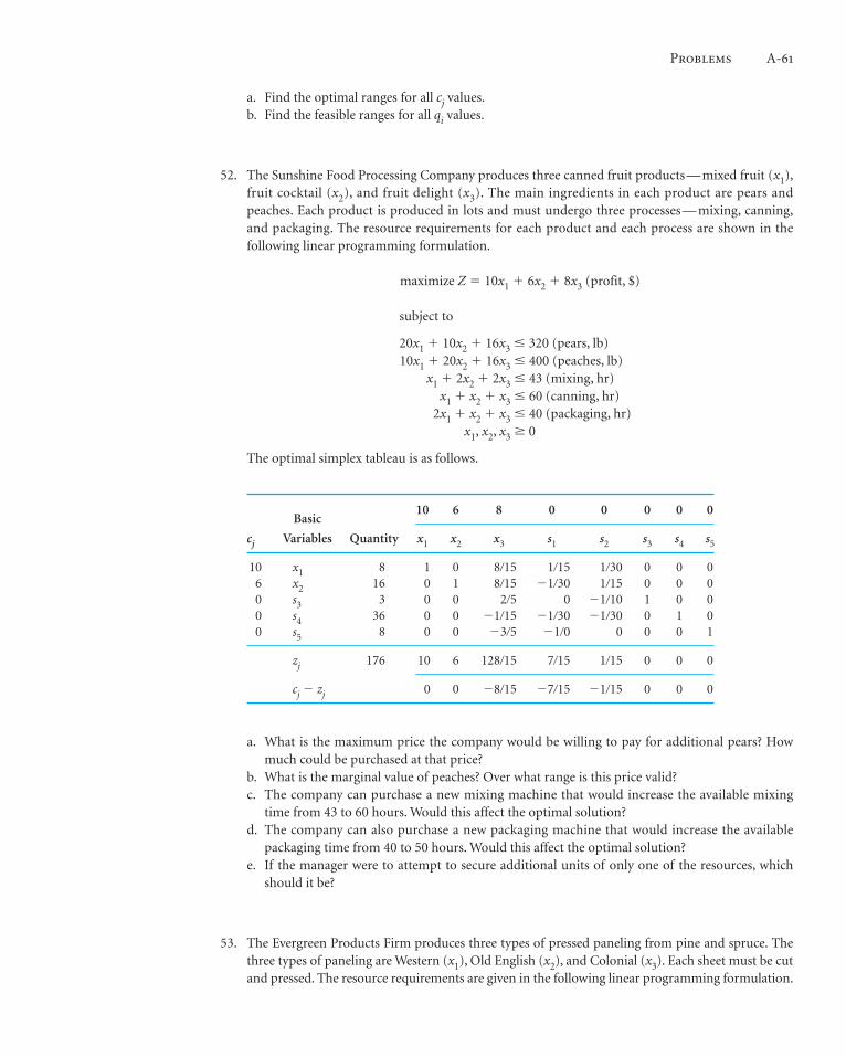
Problems A-61

a. Find the optimal ranges for all cj values.b. Find the feasible ranges for all qi values.

52. The Sunshine Food Processing Company produces three canned fruit products — mixed fruit (x1),fruit cocktail (x2), and fruit delight (x3). The main ingredients in each product are pears andpeaches. Each product is produced in lots and must undergo three processes — mixing, canning,and packaging. The resource requirements for each product and each process are shown in thefollowing linear programming formulation.


subject to

20x1 � 10x2 � 16x3 � 320 (pears, lb)10x1 � 20x2 � 16x3 � 400 (peaches, lb)

x1 � 2x2 � 2x3 � 43 (mixing, hr)x1 � x2 � x3 � 60 (canning, hr)

2x1 � x2 � x3 � 40 (packaging, hr)x1, x2, x3 0

The optimal simplex tableau is as follows.

Basic10 6 8 0 0 0 0 0

cj Variables Quantity x1 x2 x3 s1 s2 s3 s4 s5

10 x1 8 1 0 8�15 1�15 1�30 0 0 06 x2 16 0 1 8�15 �1�30 1�15 0 0 00 s3 3 0 0 2�5 0 �1�10 1 0 00 s4 36 0 0 �1�15 �1�30 �1�30 0 1 00 s5 8 0 0 �3�5 �1�0 0 0 0 1

zj 176 10 6 128�15 7�15 1�15 0 0 0

cj � zj 0 0 �8�15 �7�15 �1�15 0 0 0

a. What is the maximum price the company would be willing to pay for additional pears? Howmuch could be purchased at that price?

b. What is the marginal value of peaches? Over what range is this price valid?c. The company can purchase a new mixing machine that would increase the available mixing

time from 43 to 60 hours. Would this affect the optimal solution?d. The company can also purchase a new packaging machine that would increase the available

packaging time from 40 to 50 hours. Would this affect the optimal solution?e. If the manager were to attempt to secure additional units of only one of the resources, which

should it be?

53. The Evergreen Products Firm produces three types of pressed paneling from pine and spruce. Thethree types of paneling are Western (x1), Old English (x2), and Colonial (x3). Each sheet must be cutand pressed. The resource requirements are given in the following linear programming formulation.



subject to

5x1 � 4x2 � 4x3 � 200 (pine, lb)2x1 � 5x2 � 2x3 � 160 (spruce, lb)

x1 � x2 � 2x3 � 50 (cutting, hr)2x1 � 4x2 � 2x3 � 80 (pressing, hr)

x1, x2, x3 0


Basic4 10 8 0 0 0 0

cj Variables Quantity x1 x2 x3 s1 s2 s3 s4

0 s1 80 7�3 0 0 1 0 �4�3 �2�30 s2 70 �1�3 0 0 0 1 1�3 �4�38 x3 20 1�3 0 1 0 0 2�3 �1�6

10 x2 10 1�3 1 0 0 0 �1�3 1�3

zj 260 6 10 8 0 0 2 2

cj � zj �2 0 0 0 0 �2 �2

a. What is the marginal value of an additional pound of spruce? Over what range is this valuevalid?

b. What is the marginal value of an additional hour of cutting? Over what range is this value valid?c. Given a choice between securing more cutting hours or more pressing hours, which should

management select? Why?d. If the amount of spruce available to the firm were decreased from 160 to 100 pounds, would this

reduction affect the solution?e. What unit profit would have to be made from Western paneling before management would con-

sider producing it?f. Management is considering changing the profit of Colonial paneling from $8 to $13. Would this

change affect the solution?

54. A manufacturing firm produces four products. Each product requires material and machine pro-cessing. The linear programming model formulated to determine the number of product 1 (x1),product 2 (x2), product 3 (x3), and product 4 (x4) to produce is as follows.

maximize Z � 2x1 � 8x2 � 10x3 � 6x4 (profit, $)

subject to

2x1 � x2 � 4x3 � 2x4 � 200 (material, lb)x1 � 2x2 � 2x3 � x4 � 160 (machine processing, hr)

x1, x2, x3, x4 0

Problems A-63


Basic2 8 10 6 0 0

cj Variables Quantity x1 x2 x3 x4 s1 s2

6 x4 80 1 0 2 1 2�3 �1�38 x2 40 0 1 0 0 �1�3 2�3

zj 800 6 8 12 6 4�3 10�3

cj�zj �4 0 �2 0 �4�3 �10�3

What is the marginal value of an additional pound of material? Over what range is this value valid?

a the simplex solution method - winonacourse1.winona.edu/mwolfmeyer/ba340/module_a.pdf · only...

Documents