Æ the 1976/77 transition in precipitation over the...

Huei-Ping Huang Æ Richard Seager Æ Yochanan Kushnir

The 1976/77 transition in precipitation over the Americas and theinfluence of tropical sea surface temperature

Received: 23 September 2004 / Accepted: 9 February 2005 / Published online: 11 May 2005� Springer-Verlag 2005

Abstract Most major features of the interdecadal shift inboreal winter-spring precipitation over the Americancontinents associated with the 1976–1977 transition arereproduced in atmospheric general circulation model(GCM) simulations forced with observed sea surfacetemperature (SST). The GCM runs forced with globaland tropical Pacific SSTs produce similar multidecadalchanges in precipitation, indicating the dominant influ-ence of tropical Pacific SST. Companion experimentsindicate that the shift in mean conditions in the tropicalPacific is responsible for these changes. The observedand simulated ‘‘post- minus pre-1976’’ difference in Jan–May precipitation is wet over Mexico and the southwestU.S., dry over the Amazon, wet over sub-AmazonianSouth America, and dry over the southern tip of SouthAmerica. This pattern is not dramatically different froma typical El Nino-induced response in precipitation.Although the interdecadal (post- minus pre-1976) andinterannual (El Nino�La Nina) SST anomalies differ indetail, they produce a common tropics-wide tropo-spheric warmth that may explain the similarity in theprecipitation anomaly patterns for these two time scales.An analysis of local moisture budget shows that, exceptfor Mexico and the southwest U.S. where the inter-decadal shift in precipitation is balanced by evaporation,elsewhere over the Americas it is balanced by a shift inlow-level moisture convergence. Moreover, the moistureconvergence is due mainly to the change in low-levelwind divergence that is linked to low-level ascent anddescent.

1 Introduction

The influences of tropical sea surface temperature(SST) anomalies on the precipitation over the Ameri-can continents on the interannual time scale are wellknown (Ropelewski and Halpert 1987). During ElNino, the southern edge of the U.S. and northernMexico are typically wetter, northern Brazil and theCaribbean are drier, and southeastern South Americais wetter than normal. The simultaneous occurrencesof interannual climate anomalies in both hemispheresreflect their common origin in the tropical SSTanomaly (Seager et al. 2003). Atmospheric generalcirculation models (GCMs) forced by El Nino SSTanomalies have successfully simulated the inter-Amer-ican precipitation pattern, an important basis for thetwo-tier system of seasonal prediction (e.g., Goddardet al. 2001). Looking for further evidence of thetropical control of midlatitude precipitation, recentstudies have qualitatively reproduced prolonged NorthAmerican droughts with atmospheric GCMs forced byobserved tropical SST (Hoerling and Kumar 2003;Schubert et al. 2004; Seager et al. 2005, manuscriptsubmitted to J. Climate). Following these develop-ments, a natural and important extension that we willpursue in this study is to investigate the relationshipbetween the interdecadal changes in tropical SST andprecipitation over the Americas.

Unlike interannual variability that can be explainedby recurring El Ninos, the causes of multidecadal vari-ability or trends in tropical SST remain a matter ofinvestigation, with possibilities ranging from internalocean–atmosphere dynamics (e.g., Gu and Philander1997; McPhaden and Zhang 2002; Seager et al. 2004;Karspeck et al. 2004), changes in the characteristics ofEl Nino (Fedorov and Philander 2001), to greenhouse-gas forcing (e.g., Cane et al. 1997; Boer et al. 2004).Leaving the ocean dynamics aside, this work aims toinvestigate how the atmosphere and the precipitationover land in the American sector respond to the inter-

H.-P. Huang (&) Æ R. Seager Æ Y. KushnirLamont-Doherty Earth Observatoryof Columbia University, 61 Route 9W,Palisades, NY, 10964 USAE-mail: [email protected]: +1-845-3658736

Climate Dynamics (2005) 24: 721–740DOI 10.1007/s00382-005-0015-6

decadal changes in SST when the latter are given. Theobserved interdecadal changes in tropical SST and manyatmospheric variables (e.g., global angular momentum,Huang et al. 2003; tropically averaged 200 hPa height,Kumar et al. 2004) for the second half of the twentiethcentury are not smooth but are distinguished by a‘‘shift’’ in the late 1970s (Trenberth 1990), often calledthe 1976–1977 transition. The fact that the post- andpre-1976 periods have distinctive means provides aconvenient setting for our investigation of the multi-decadal SST-precipitation relationship. Our strategy isto bypass an analysis of the detailed temporal evolution,containing all time scales, of the SST and precipitationfor the second half of the twentieth century, and insteadfocus on the difference between the post- and pre-1976epoch means. As an extension of previous GCM studies,we will determine whether an AGCM forced by thedifference in tropical SST across the 1976 transition cansimulate the corresponding interdecadal shift in precip-itation over the Americas.

Using two GCMs different from the one used in thepresent study, Kumar et al. (2004) have recently lookedat some aspects of the SST-precipitation relationship onthe interdecadal time scale. They pointed out that, de-spite an increase in the tropics-wide temperature asso-ciated with the increase in tropical SST for 1950–2000,the precipitation over land in the tropics has decreased.This feature, which we will confirm, suggests that thechange in precipitation could be more than just anintensification of the local recycling of water, namely, anincrease in temperature leads to more evaporation that isbalanced by more precipitation back to surface. As anew contribution to this problem, we will analyze notonly the SST and precipitation, but also all terms in thelocal moisture budget associated with the 1976 transi-tion. This will clarify whether the changes in regionalprecipitation are balanced by evaporation or by changesin atmospheric moisture transport. Due to deficiencies inthe observations for atmospheric moisture field in thepre-1976 era (and a still large uncertainty in the decadalmeans of moisture in the post-satellite era, e.g., Allanet al. 2002), we will rely on GCM simulations for themoisture budget analysis.

Since some of the strongest El Nino events in thetwentieth century occurred in the post-1976 period, thedifference between the means of the post- and pre-1976epochs could be due partly to the rectified effect of ElNino. Outside the tropical Pacific, the SSTs in otherocean basins may also influence the precipitation overthe Americas. To shed light on these possibilities, we willanalyze GCM simulations forced with global and trop-ical Pacific SSTs, and with the SST forcing including andexcluding interannual variability (as detailed in Sect. 3).The basic features of the multidecadal changes in trop-ical SST are shown in Sect. 2. The model and GCMexperiments are described in Sect. 3. The ‘‘post- minuspre-1976’’ differences in precipitation and moisturebudget over the Americas are analyzed in Sect. 4, fol-lowed by additional discussions on the interdecadal

SST-precipitation relationship in Sects. 5, 6, and 7 andconclusions in Sec. 8.

2 SST and the 1976 transition

In this study, July 1961–June 1976 and July 1976–June1998 are chosen to define the pre-1976 and post-1976epochs. The choice of 1998 as the end of the post-76 erais guided by an apparent ‘‘reversal’’ of the post-1976trend in the precipitation of the Americas that occurredin mid-1998 (see Sect. 7). The choice of 1961 as the otherend point is somewhat arbitrary, but extending it to 1956leads to qualitatively similar results in our GCMexperiments (the ‘‘SCYC’’ runs to be discussed shortly).That these choices are meaningful is illustrated inFig. 1a–c, the Jan–May SST ‘‘anomalies’’ (defined as thedeparture from the 1871–1999 climatology using theHadISST1 data set, Rayner et al. 2003) for the post- andpre-1976 periods and their difference. Both Fig. 1a and bexhibits a common pattern with the largest SST anom-alies in the central/eastern Pacific and just south of theequator. Moreover, the post- and pre-1976 SST anom-alies in Fig. 1a and b have the same pattern but oppositesigns over most of the Indo-Pacific sector, rendering itmeaningful to consider the two epochs the ‘‘positive’’and ‘‘negative’’ phases of a multidecadal oscillation,with 1976 being the turning point.

The ‘‘post- minus pre-1976’’ SST difference field,shown in Fig. 1c, is positive over most of the Indo-Pa-cific sector, except for the two off-equatorial minima inthe western Pacific. The most distinctive feature is,again, a maximum south of the equator in the central/

a

b

c

Fig. 1 The anomaly of Jan–May SST, defined as the departurefrom 1871–1999 long-term mean, for a post-1976 epoch (July 1976–June 1998), b pre-1976 epoch (July 1961–June 1976), c thedifference of a and b. Contour interval 0.1�C, negative dashed.Areas with the absolute value of SST anomaly greater than 0.1�Care filled with red (positive) and blue (negative) colors

722 Huang et al.: The 1976/77 transition in precipitation over the Americas and the influence of tropical sea surface temperature

eastern Pacific. On the interannual time scale, El Nino inthe equatorial Pacific influences the SST elsewherethrough an ‘‘atmospheric bridge’’ (Alexander et al.2001), producing SST anomalies of the same sign as theNINO3/3.4 index in the Indian Ocean and opposite signin the North Pacific. Qualitatively, this remains true inFig. 1c, but the Indian Ocean SST anomaly has becomestronger relative to the NINO3/3.4 SST anomaly in theequatorial Pacific. These differences between the inter-annual and interdecadal SST anomaly patterns are alsonoted by Deser et al. (2004), who further showed theconnection between the tropical and North Pacificoceans on the interdecadal time scale. The warmingcomponent in Fig. 1c also broadly resembles the SSTtrend simulated by some coupled GCMs forced with anincreased greenhouse gas concentration (e.g., Knutsonand Manabe 1995; Huang et al. 2001; Boer et al. 2004).The observed epoch difference in Fig. 1c could be amixture of both internal variability and global warmingtrend.

To simplify the problem, the GCM simulations inthis study will be forced by either tropical Pacific orglobal SSTs, without a further division into differentbasins. The interdecadal shift in SST has an annual cy-cle. To further narrow the focus, we will analyze theprecipitation and moisture budget for the boreal winter–spring season.

3 Models and data

The AGCM used in this study is the National Center forAtmospheric Research (NCAR) Community ClimateModel Version 3.10 (CCM3.10), with minimal modifi-cations for executions on our local computing facilities.The model has 18 vertical levels and a T42 resolution.Three sets of GCM simulations are performed. ThePacific Ocean Global Atmosphere coupled with MixedLayer ocean (POGA-ML) runs consist of 16 ensemblemembers for 1856–2000, with the model forced by ob-served SST over the tropical Pacific (including the wes-tern Pacific but excluding the Indian Ocean) and coupledto a simple mixed layer ocean elsewhere as detailed inAppendix 1. The global ocean global atmosphere(GOGA) runs include 48 ensemble members for 1959–1999 (16 members extended to 2004) forced by observedglobal SST. The 1961–1999 segments from the POGA-ML and GOGA runs are used in most of our analysis.The SCYC (abbreviation for ‘‘repeated seasonal cycle’’)experiments consist of a pair of 30-year AGCM runs,each forced with a repeated seasonal cycle of global SSTconstructed from the means of the post- and pre-1976epochs. The POGA-ML and GOGA runs producesubstantial interannual variability due to El Nino.Compared to that, the interannual variability in the

a b

dc

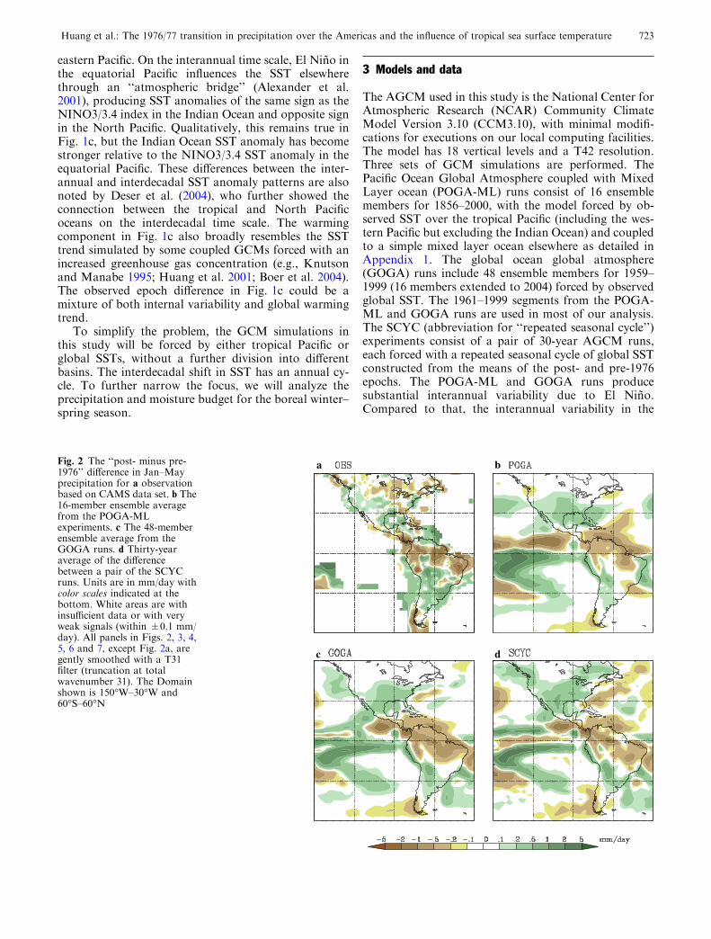
Fig. 2 The ‘‘post- minus pre-1976’’ difference in Jan–Mayprecipitation for a observationbased on CAMS data set. b The16-member ensemble averagefrom the POGA-MLexperiments. c The 48-memberensemble average from theGOGA runs. d Thirty-yearaverage of the differencebetween a pair of the SCYCruns. Units are in mm/day withcolor scales indicated at thebottom. White areas are withinsufficient data or with veryweak signals (within ±0.1 mm/day). All panels in Figs. 2, 3, 4,5, 6 and 7, except Fig. 2a, aregently smoothed with a T31filter (truncation at totalwavenumber 31). The Domainshown is 150�W–30�W and60�S–60�N

Huang et al.: The 1976/77 transition in precipitation over the Americas and the influence of tropical sea surface temperature 723

SCYC experiments consists of only internal variabilitythat is further suppressed after a 30-year average.

Since long-term (including the pre-1976 era) obser-vations of precipitation exist mainly over land, the ver-ification of model simulations will be based onprecipitation over the American continents. Unlessotherwise noted, the CAMS station data interpolatedonto a 2�·2� grid produced by NOAA Climate Predic-tion Center (http://www.cpc.ncep.noaa.gov) is used forprecipitation.

4 Interdecadal shift in precipitation and moisture budget

Precipitation

The ‘‘post- minus pre-1976’’ difference in Jan–Mayprecipitation is shown in Fig. 2a–d for the observationsand the POGA-ML, GOGA, and SCYC runs. The re-sults for POGA-ML and GOGA are the ensembleaverage of 16 and 48 runs, respectively, while that forSCYC is the difference between a pair of 30-year per-petual post-1976 and pre-1976 runs. To first order, theGCM reproduces many observed features of the inter-decadal shift in precipitation over the American conti-nents, including dry anomalies over the Amazon and thesouthern tip of South America, wet anomalies over sub-Amazonian South America, Mexico, and the southwestU.S. Over these regions, the POGA-ML and GOGAruns produce very similar structures in precipitation,indicating the dominant impact of tropical Pacific SST.This result supports the emerging thought of the controlof global climate by tropical oceans advanced by recentstudies (Hoerling and Kumar 2003, Schneider et al.2003; Seager et al. 2003; Schubert et al. 2004; Seageret al. 2005), although the emphases of these studies arenot restricted to the Pacific (e.g., Hoerling and Kumar2003 noted the contribution of the Indian Ocean SSTAto the post-1998 North American drought; Schneideret al. 2003 found a substantial influence of tropicalAtlantic SST on the trend in precipitation over tropical

South America for the second half of the twentiethcentury). The SCYC runs, designed to exclude the rec-tified effect of interannual variability, also producesimilar results in precipitation.

Despite the similarity between the POGA-ML andGOGA/SCYC runs, some second order differences arenoticeable. For example, over the northeast coast ofBrazil the precipitation anomalies are wet in POGA-MLbut dry in GOGA, SCYC, and observations. Thesedetails might be related to the differences in the SSTs inthe adjacent Atlantic Ocean (e.g., Giannini et al. 2004),i.e., the POGA-ML model simulation of tropicalAtlantic SST anomalies is different from observations.Note as well a discrepancy between the simulated (for allthree types of runs) and observed precipitation over theGreat Lakes region and the northeast U.S., where themodel is too wet during the post-1976 period. Otherwise,the rest of the simulated precipitation patterns inFig. 2b–d are very robust, as they can be reproduced byretaining only a small number of ensemble members inthe ensemble means for POGA-ML and GOGA, or asmall number of years in the time mean for SCYC runs(not shown). A more detailed discussion on statisticalsignificance is in Appendix 2.

Recalling that the canonical El Nino signal in pre-cipitation is wet over the southern edge of the U.S., dryover northern South America, and wet over the centralSouth America (Ropelewski and Halpert 1987), we notethat in these regions the sign of the interannual signal isthe same as the interdecadal one shown in Fig. 2. For aquick reference, the ‘‘warm minus cold’’ ENSO com-posite of Jan–May precipitation anomalies from thePOGA-ML and GOGA runs is shown in Fig. 3. Thesimilarity between the interdecadal and interannualprecipitation signals is likely due to the broad similaritybetween the interdecadal and interannual (El Nino) SSTanomalies, to be discussed further in Sect. 6. Neverthe-less, there are non-trivial differences between the inter-annual and interdecadal precipitation patterns. In thelatter, the wet anomaly in the southern edge of NorthAmerica penetrates much deeper into the southwest

a bFig. 3 The warm minus coldENSO composite of Jan–Mayprecipitation for the ensemblemeans of a POGA-ML runs. bGOGA runs. Color scales areindicated at the bottom. Thecomposite is based on six majorEl Ninos (Jan-May of 1966,1969, 1983, 1987, 1992, and1998) and six major La Ninas(1968, 1971, 1974, 1976, 1985,and 1989), normalized by theJan–May average of NINO3.4index. The composite is doneafter the time series ofprecipitation at each grid pointis detrended with a high passfilter


U.S., while in the former it is centered to the southeastaround the Gulf coast and Florida (Ropelewski andHalpert 1987). The dry region in the north, and wetregion in central South America, are broader for theinterdecadal anomalies. Also noteworthy is a dryanomaly over the southern tip of South America in bothobserved and simulated multidecadal precipitation pat-terns in Fig. 2. At first, it appears to be a unique featureof the interdecadal variability since it has not beenrecorded as part of the canonical ENSO signal in pre-cipitation (Ropelewski and Halpert 1987). However, wedid find a trace of dryness in this region in the simulatedEl Nino precipitation anomalies in the POGA-ML andGOGA runs. We postpone further comparisons of theinterannual and interdecadal signals to Sects. 5 and 6.

Investigating the decadal variability (with period T>7 years) of precipitation over land, Cayan et al. (1998;see their Fig. 10) found an apparent global correlationpattern for precipitation anomalies that broadly resem-bles our pattern of the multidecadal shift in the Ameri-can sector. When the precipitation anomaly is wet in thesouthern/southwest U.S. and Mexico, it is dry/wet/dryover northern/central/southern South America. Using 6-year low-pass filtered data, Schubert et al. (2004, seetheir Fig. 2) also found a similar correlation pattern butwith a diminished dry spot over the southern tip ofSouth America. Although the frequency band consid-

ered by Cayan et al. (1998) and Schubert et al. (2004) forthe low-frequency variability is broader (including fluc-tuations with relatively shorter periods) than ours, thepartial overlap between the two may explain the simi-larity in the precipitation patterns. Most importantly,since we are able to simulate this inter-American pre-cipitation pattern with the POGA-ML runs, the corre-lation between the precipitation anomalies in North andSouth America is likely due to the fact that they have acommon origin in the tropical Pacific SST.

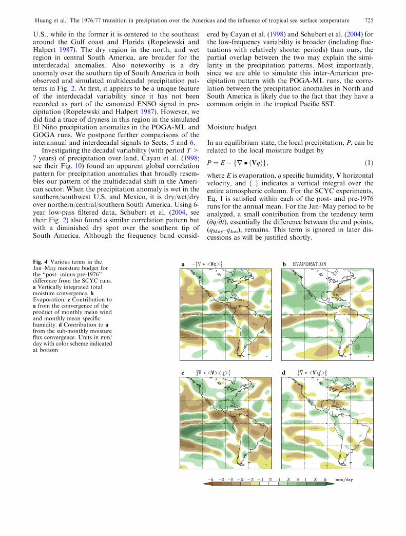
Moisture budget

In an equilibrium state, the local precipitation, P, can berelated to the local moisture budget by

P ¼ E � fr � ðVqÞg; ð1Þ

where E is evaporation, q specific humidity, V horizontalvelocity, and { } indicates a vertical integral over theentire atmospheric column. For the SCYC experiments,Eq. 1 is satisfied within each of the post- and pre-1976runs for the annual mean. For the Jan–May period to beanalyzed, a small contribution from the tendency term(¶q/¶t), essentially the difference between the end points,(qMay–qJan), remains. This term is ignored in later dis-cussions as will be justified shortly.

a b

c d

Fig. 4 Various terms in theJan–May moisture budget forthe ‘‘post- minus pre-1976’’difference from the SCYC runs.a Vertically integrated totalmoisture convergence. bEvaporation. c Contribution toa from the convergence of theproduct of monthly mean windand monthly mean specifichumidity. d Contribution to afrom the sub-monthly moistureflux convergence. Units in mm/day with color scheme indicatedat bottom


Denoting the difference between the post- and pre-1976 epoch means of a variable X as

dX � XC, POST76� XC, PRE76

; ð2Þ

where XC indicates the mean of the post- or pre-1976period, the shift in precipitation across the 1976 transi-tion can be related to those in the other terms in themoisture budget by

dP ¼ dE � dfr � ðVqÞg: ð3Þ

Here, an increase in local precipitation could be ex-plained by an intensified moisture convergence or anincrease in local evaporation. This distinction mayprovide useful clues to the relative importance of dif-ferent dynamical/thermodynamical processes pertinentto dP.

The terms �d{�•(Vq)} and dE from the SCYC runsfor Jan–May are shown in Fig. 4a and b. Over Mexicoand the southwest U.S., the increase in precipitation ispartly balanced by an increase in evaporation, implyingan intensification of local moisture recycling. Elsewhere,the dP (see Fig. 2d) is balanced mainly by moistureconvergence/divergence, �d{�•(Vq)}. The change inmoisture convergence is also important over Mexico andthe southwest U.S. The dE shown in Fig. 4b is directlycomputed from the model output of latent heat fluxes.However, one obtains an almost identical dE if it isdiagnosed from Eq. 3, another indication that the ig-nored term in Eq. 3, d(qMay–qJan), is small. (Taking thedifference between the two estimates of dE as a measureof the tendency term, the variance of the latter is lessthan 10% of that of dE itself.) Note that this term isnonzero only if there is a shift in the annual cycle ofprecipitation. That it is small indicates that a shift in theseasonal cycle is not the major cause for the interdecadalshift in Jan–May precipitation.

The moisture convergence shown in Fig. 4a is thetotal, with contributions from sub-monthly and monthlyto longer time scales. In the SCYC experiments, the totalmoisture flux Vq is saved monthly (as the monthly

mean), along with the monthly means of V and q.Denoting the monthly mean and the ‘‘departure frommonthly mean’’ of a variable X as <X> and X¢, thetotal moisture flux convergence can be decomposed into

�r �\Vq >¼ �r � ð\V >\q >Þ � r � ð\V0q0 >Þ;ð4Þ

with the last term being the contribution from the sub-monthly processes that can be diagnosed from the othertwo. Figure 4c and d shows the post- minus pre-1976differences in the two terms in the r.h.s. of Eq. 4. Thesub-monthly term is much smaller over land and overmost of the ocean. Hereafter, we will focus on thedominant term, ��•(<V><q>). To completelyexclude the contribution from interannual variability,we will again consider the SCYC case, but note that thedifferences in ��•(<V><q>) across the 1976 transi-tion simulated by the POGA-ML and GOGA runs,shown in Fig. 5a and b, are similar to that obtained bythe SCYC experiments.

Detail of the shift in moisture convergence

The interdecadal shift in moisture convergence could bedue to changes in the domain-averaged moisture con-centration, moisture gradient, total (advective) wind, orthe wind divergence. Separating these possibilities wouldprovide additional clues to the connection between thelocal moisture budget and large-scale circulation. Forconciseness, in the following the angled bracket < >will be eliminated, with all the V and q understood asmonthly means. The symbol for vertical integral, { } isalso eliminated but is implied. A quadratic term writtenas XY here is equivalent to {<X><Y>} in the pre-ceding sections. The post- minus pre-1976 difference inmoisture convergence can be rewritten as

�dr � Vqð Þ ¼ �d V � rqð Þ�ðAÞ

d qr � Vð ÞðBÞ ; ð5Þ

a bFig. 5 Same as Fig. 4c but for athe ensemble mean of thePOGA-ML runs. b Theensemble mean of the GOGAexperiments. Units in mm/daywith color scales indicated atbottom


where dX and XC are the ‘‘post- minus pre-1976’’ dif-ference and the pre-1976 epoch mean of X. Theexpansion in Eq. 6 is intuitive but a more rigorousderivation can be found in Appendix 3. The higher-order terms in Eq. 6 include quadratic terms of‘‘dXdY’’ type and the contribution from interannualvariability within the post- and pre-1976 periods(Appendix 3). The latter can be conveniently ignored asit is small for the SCYC runs.

Equations 5 and 6 provide a useful decomposition ofthe interdecadal shift in the total moisture convergence.Term (A) represents the effect of moisture convergencedue to advection across the moisture gradient. In thiscase, the wind vector V includes both rotational anddivergent components but a further decomposition (notshown) indicates that the contribution of the rotationalwind is significant. Term (B) represents the effect of winddivergence/convergence. The wind vector that is relevant

� �r � Vqð Þ ¼�VC � rð�qÞ�

ðA1Þð�VÞ � rqC�ðA2Þ

ð�qÞr �VC�ðB1Þ

qCr � ð�VÞðB2Þ

þ higher order terms ð6Þ

a b

c d

e f

Fig. 6 The major terms in thedecomposition of the ‘‘post-minus pre-1976’’ difference inthe Jan–May verticallyintegrated moistureconvergence in Eq. (6), from theSCYC experiment. a Term(A1). b Term (A2). c Term (B1).d Term (B2). e Sum of a–d. Thevertical integrals for a–d are forthe entire atmospheric column.(f) Same as (d) but with only thelowest five levels retained in thevertical integral. Units in mm/day, with color scales indicatedat bottom


to term (B) is its divergent component. Further, the sub-term (A1) in Eq. 6 represents the effect of the changes inmoisture gradient when the total advective (rotationalplus divergent) wind field is fixed. Term (A2) representsthe contribution from the changes in total wind fieldwith the moisture gradient fixed. Term (B1) representsthe effect of the changes in the domain-averaged mois-ture with a fixed divergent wind, and term (B2) the effectof the changes in the wind divergence with fixed mois-ture. Terms (A1)–(B2) are shown in Fig. 6a–d (remem-ber that they are the vertical integrals). In SouthAmerica and much of the Caribbean and CentralAmerica, term (B2) dominates such that the sum of the

four terms, shown in Fig. 6e, is almost identical toFig. 6d. (That Fig. 6e resembles Fig. 4c reassures us thatthe higher-order terms in Eq. 6 are indeed small.) Thus,for these regions, the interdecadal shift in the totalmoisture convergence is due to the changes in thedivergent component of the wind.

Given the dramatic decrease in specific humiditywith height, the column-integrated moisture conver-gence in Fig. 6a–d comes mainly from the lowest fewlevels. This is illustrated in Fig. 6f, the same term as inFig. 6d but with only the lowest five levels in the model(correspond approximately to 1,000–750 hPa over a flatsurface) retained in the vertical integral. Clearly, the

a b

c d

e f

Fig. 7 Same as Fig. 6 but forthe ensemble mean of theGOGA runs


decrease in precipitation over the Amazon is balancedby a decrease in low-level wind convergence, corre-sponding to a weakening of the climatological ascentover this region. The closeness of Fig. 6d and f alsoextends to other terms (not shown) in Eq. 6, such thatour previous discussion of the moisture and winds canbe replaced by that of the low-level moisture and low-level winds.

Figure 7 shows the counterpart of Fig. 6 for theGOGA runs. Just like precipitation, the GOGA andSCYC runs produce similar patterns for the individualterms in the moisture budget. The POGA-ML runs alsoproduce similar results for moisture budget but are notshown for brevity. Again, the dominant term is (B2) inEq. 6, due to the changes in low-level wind divergence.

By mass continuity, the low-level divergence and con-vergence are related to descent and ascent in the lower tomiddle troposphere.

Over Mexico and the southwest U.S., the four termsin Eq. 6 have comparable amplitudes but their sum isnot large. As already shown in Fig. 4, in this region theincrease in precipitation is balanced mainly by anincrease in evaporation. Over land, the changes inevaporation involve complicated processes related to soilmoisture. Over the mountainous region in the southwestU.S., the Jan–May evaporation also depends on themelting of snow accumulated in the preceding fall andearly winter. The change in moisture convergenceremains important but clearly the interdecadal shiftinvolves a complex interaction between the remotely

a d

b e

c f

Fig. 8 The ‘‘post- minus pre-1976’’ difference in the Jan–May 200 hPa zonal wind for aPOGA-ML; b GOGA; c SCYCexperiments. d–f are the same asa–c but for the 200-hPastreamfunction. Contourinterval 1 m s�1 for zonal wind,1·106 m2 s�1 forstreamfunction. Positive andnegative contours are in red andblue, with zero contoursomitted


forced changes in atmospheric circulation and the localground hydrology.

Over the northeast U.S. and Great Lakes region, thesimulated interdecadal shift in precipitation is balancedby moisture convergence, although the fact that all ofthe sub-terms in Eq. 6, except (B1), and the sub-monthlymoisture convergence (Fig. 4d) have about equal andnon-negligible amplitudes renders a clear interpretationof the interdecadal pattern difficult. Note that this is alsothe region with a notable discrepancy between the ob-served and simulated interdecadal shift in precipitation,with the latter wetter than the former.

The decomposition of moisture transport in Eqs. 4, 5,6 is useful for analyzing not only interdecadal variabilitybut also climate changes on longer time scales. It isworth noting that, in a simple model study, Chou andNeelin (2004) found that the change in precipitationover land caused by doubled CO2 is balanced mainly bythe local moisture transport due to changes in massdivergence, a term analogous to (B2) in our Eq. 6.

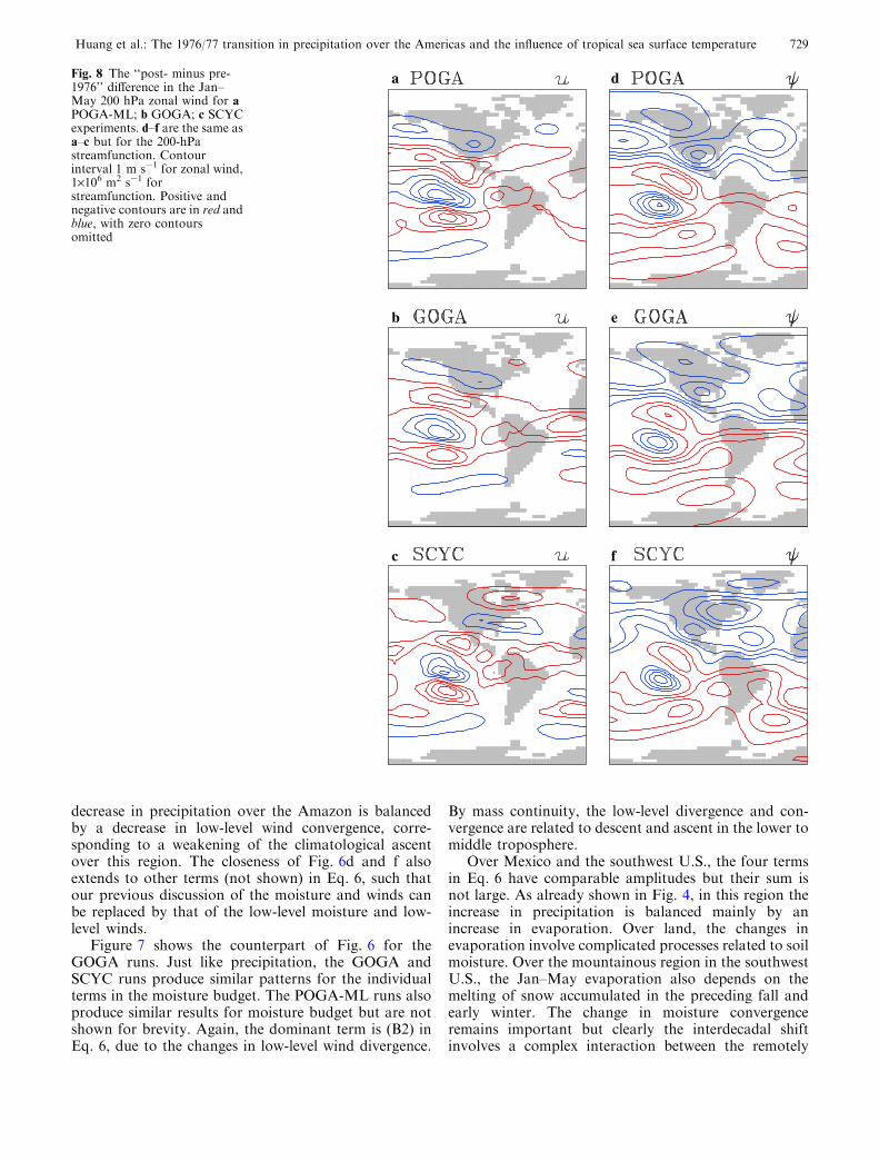
5 Upper-level circulation

Although the interdecadal changes in precipitation overthe Americas are more intimately related to low-levelconvergence/divergence or ascent/decent, for complete-ness we will present some results for the upper-levelcirculation, useful for a subsequent discussion on inter-annual and interdecadal variability. Figure 8a–c showsthe post- minus pre-1976 differences in the 200 hPa zo-nal wind from the POGA-ML, GOGA, and SCYCexperiments. A hemispherically symmetric and zonallyelongated pattern, with an acceleration of subtropicaljets in both hemispheres, can be readily identified in

Fig. 8a and b. This pattern is similar to the typical zonalwind response to El Nino (e.g., Seager et al. 2003; Lauet al. 2005). Since the POGA-ML and GOGA runs in-clude the rectified effect of interannual variability, thefact that there are more strong El Ninos (La Ninas) inthe post- (pre-) 1976 epoch might contribute to thestructures in Fig. 8a and b. However, this pattern is alsopresent (but somewhat weakened) in Fig. 8c for theSCYC runs forced by the interdecadal SST anomaly.This indicates that the zonal wind response is not sen-sitive to the detail of tropical SST anomalies, a pointthat will be revisited in Sec. 6.

The post- minus pre-1976 differences in the 200 hPastreamfunction for the POGA-ML, GOGA, and SCYCruns are shown in Fig. 8d–f. Streamfunction, instead ofgeopotential height, is used here to enhance structures inthe tropics. (See e.g., Hsu and Lin 1992, for a discussionof global teleconnections based on streamfunction. Sincethe anomalous geopotential and streamfunction areapproximately related by dF �fdw, where f is theCoriolis parameter, in the lower latitudes the geopo-tential height anomaly is flatter.) In the streamfunctionfield, a pair of Rossby wave trains emanating from thetropical Pacific to the midlatitudes of both hemispheresare more clearly seen as responses to the tropical SSTanomalies (e.g., Trenberth et al. 1998). These wave trainsare not significantly different among the SCYC andPOGA-ML/GOGA runs.

Notably, even with its maximum located south of theequator, the interdecadal SST anomaly (Fig. 1c) pro-duces a cross-equatorial wave train that propagates intothe Northern Hemisphere. This can be understood intwo ways: first, in boreal winter the longitudinal sectoron the equator from 150�W–90�W is predominantlywesterly, allowing a pathway for cross-equatorial wave

a

b

c

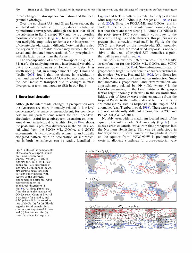
Fig. 9 a One of the componentsof the anomalous (post- minuspre-1976) Rossby wavesource,��•{dVv(fC+f)}, at200 hPa for Jan–May. b Post-minus pre-1976 divergence at200 hPa. c Contours of the 200-hPa climatological absolutevorticity superimposed withvectors of the divergentcomponent of horizontal windcorresponding to theanomalous divergence inFig. 9b. All three panels arefrom the ensemble average ofGOGA runs. Contour intervalis arbitrary for a and b, and0.2W (where W is the rotationrate of the Earth) for (c). Blue isnegative for all panels. Zerocontours are suppressed for (a)and (b) but retained for (c) toshow the dynamical equator


propagation (Webster and Holton 1982; Hsu and Lin1992). Second, the Rossby wave source (RWS, Sard-eshmukh and Hoskins 1988) responsible for the gener-ation of upper-level Rossby waves can spread beyondthe confines of the SST anomaly itself (see Sardeshmukhand Hoskins 1988). In our problem, the post- minus pre-1976 difference in RWS, dRWS, can be produced byboth positive and negative divergence anomalies asso-ciated with anomalous precipitation (Fig. 2c). To illus-trate, Fig. 9a shows one of the major components ofdRWS, dRWS1=�� • {dVv(fc+f)}, due to the anom-alous divergence acting on the climatological absolutevorticity at 200 hPa for Jan–May from the ensemblemean of the GOGA runs. (As usual, dX and XC repre-sent the post- minus pre-1976 difference and the pre-1976 epoch mean of X. Vv, f, and f are the divergentcomponents of horizontal wind vector, relative vorticity,and the Coriolis parameter.)

In the tropics dRWS1 is concentrated over the easternPacific, supporting our argument that the anomalousRossby wave trains shown in Fig. 8 originate from thisregion. (In Fig. 9a, a few centers of dRWS1 also exist inmidlatitude. They are partly related to jet exits and en-trances (e.g., Nakamura 1993; Robinson 1994) andmight play a role in exciting midlatitude Rossby waves(e.g., Qin and Robinson 1993). An analysis of this partof dRWS is more complicated and is left for futurework.)

It is worth noting that, although the post- minus pre-1976 200 hPa divergence, shown in Fig. 9b, exhibits twostrong positive centers over the equatorial western Pa-cific and Indian Ocean (related to the positive SSTAsthere in Fig. 1c), the corresponding dRWS1 is not large

there. This is because the meridional gradient of abso-lute vorticity over the western Pacific and Indian Oceanis not as tight as that over the eastern equatorial Pacific,as shown in Fig. 9c. This explains the smallness (com-pared to eastern Pacific) of one of the sub-componentsof dRWS1, �dVv•�(fC+f), over the former two regions.The other sub-component, �(fC+f)�•(dVv), is also notlarge over those regions because the centers of anoma-lous divergence there nearly coincide with the dynamicalequator, the contour of fC+ f =0, as shown in Fig. 9c.

In Fig. 8, the anomalous wave trains are locatedmostly over the ocean but they intersect with theAmerican continents with a low over Mexico and thesouthwest U.S. and a trough over the southern tip ofSouth America. Although it is tempting to relate thesetwo features to the wet and dry anomalies in precipita-tion in these two regions, we instead caution that, ingeneral, upper-level highs/lows and precipitation do nothave a simple one-to-one correspondence (see e.g., Bateset al. 2001 for examples showing the disparity of thisrelationship) since the latter depends on additional fac-tors such as large-scale moisture supply, local topo-graphic lifting, etc.

Although the recently constructed ‘‘reanalysis’’ datasets include grided upper-level winds for the pre-1976period, their reliability depends on the density of upper-air observations that can be scarce especially over theoceans. A quick look at the post- minus pre-1976 dif-ference in the NCEP/NCAR reanalysis reveals no clearpatterns of the wave train over the southeast Pacificshown in Fig. 8d–f. However, records also indicate thatthere is virtually no coverage of upper-air observationsin this region for the pre-1976 period (see Fig. 5.3 of

a d

b

c

e

f

Fig. 10 The ‘‘post- minus pre-1976’’ difference in the Jan–May zonal mean zonal wind fora POGA-ML; b GOGA; cSCYC experiments. d–f are thesame as a–c but for the meanmeridional circulation (MMC)represented by the Stokesstreamfunction in meridionalplane (Peixoto and Oort 1992,chap. 7). Contour interval0.5 m s�1 for zonal mean zonalwind, 2.5·109 kg s�1 for MMC.Negative contours are dashed,and zero contours bold solid.The positive contours in d–fcorrespond to clockwisecirculation in the meridionalplane. The maxima on the mapsin d, e, and f are 26.2, 15.5, and14.0·109 kg s�1


Peixoto and Oort 1992). (For further discussions on thelimitations of the tropical circulation in reanalysis, seeTrenberth et al. 2001; Kinter et al. 2004.) To avoidmisinterpretations, we choose not to rely on thereanalysis data to verify the simulated interdecadal shiftin the upper- level circulation.

Figure 10a–c shows the post- minus pre-1976 differ-ence in the zonal mean zonal wind from the POGA-ML,GOGA, and SCYC runs. A common feature of the threepanels is the acceleration of subtropical jets at the uppertroposphere in both hemispheres. This structure isaccompanied by a zonally symmetric, tropics-wide in-crease of tropospheric temperature (see Sect. 6 andFigs. 11, 12). Again, the results for SCYC are not dra-matically different from POGA-ML/GOGA. (The dif-ference between Figs. 10c and 10a and b in the higherlatitudes in Northern Hemisphere could be due to thedifference in sea ice in the boundary forcing (seeAppendix 1) or other dynamical processes related towave-zonal mean interaction in high latitudes.) Notably,all three types of runs produce a deceleration of westerlyzonal wind at 60�S, opposite to that in the reanalysis(e.g., Thompson et al. 2000). Keeping in mind our pre-vious caution about reanalysis in the pre-1976 era, thisdifference might otherwise be related to the trends in seaice and greenhouse gas concentration. The former istreated very crudely in our GCM runs due to the lack ofobservations for the early years (Appendix 1). The trendin greenhouse gas concentration is not explicitly in-cluded in our simulations, but note that part of thegreenhouse-gas effect is embedded in the SST. In thelower latitudes, the post- minus pre-1976 difference inJan–May zonal mean zonal wind in NCEP/NCAR

reanalysis (not shown) does not exhibit a hemispheri-cally symmetric pattern of acceleration of the subtropi-cal jets simulated by the GCM. Instead, the accelerationis centered almost at the equator with its maximum inthe lower stratosphere (for useful references see Fig. 4 ofAbarca del Rio 1999; Fig. 9 of Schneider et al. 2003).This positive center is flanked by easterly anomalies inthe subtropics, with the deceleration in the SouthernHemisphere more pronounced than in the NorthernHemisphere. These differences between GCM simula-tions and reanalysis remain to be explained.

The divergent wind response to tropical SST forcinghas a zonally symmetric component that has been shownto provide a major contribution to the midlatitudemoisture budget during El Nino (Seager et al. 2005). Thezonal mean low-level divergence/convergence is associ-ated with the descent/ascent of the mean meridionalcirculation (MMC). Figure 10d–f is the same asFig. 10a–c but for the MMC. The most robust feature inFig. 10d–f is a single tropical cell with its rising branchlocated slightly south of the equator, consistent with theslightly south of the equator maximum in the inter-decadal SST pattern in Fig. 1c. The counterpart ofFig. 10d–f for the NCEP/NCAR reanalysis (not shown)exhibits a similarly oriented single-cell structure in thetropics with a comparable magnitude and with its risingbranch located in the Southern Hemisphere. Themeridional extent of that cell is slightly wider than thosesimulated by the GCM. In general, the simulated MMCresembles that in the reanalysis more closely than zonalmean zonal wind. Away from the tropics, the zonalmean MMC in the model is due to contributions fromdifferent longitudinal sectors that is not easy to interpret.

a

c

b

d

Fig. 11 The tropical (20�S–20�N) average of 200 hPaheight, shown as the departurefrom 12000 m. a The ensemblemean of POGA-ML runs. Blueline shows the 9-month low-pass- filtered time series, boldblack line the decadal-to-interdecadal componentobtained by a Fourier analysis.b Same as (a) but for GOGAruns. c Same as (a) but for theNCEP/NCAR reanalysis. d Thethree black curves from a–c areredrawn as dashed curves, witha slight shift of the POGA curveto compensate a bias (see text).The 9-month low-pass-filteredtime series (thin) and decadal/interdecadal components (bold)of the post- and pre-1976 SCYCruns are shown in blue and red,respectively


A quick estimate (not shown) reveals that, in midlati-tude, the simulated low-level zonal mean divergence/convergence is a relatively small residue of the localdivergence/convergence pertinent to the moisture con-vergence over land discussed in Sect. 4. The zonal meandivergence is only one component of the interdecadalshift in local precipitation and moisture budget over theAmericas.

6 Further remarks on interannual and interdecadalvariability

In the eastern Pacific, the major difference between theinterdecadal and interannual (El Nino) SST anomalies isthat the maximum of the former is located south of theequator. Despite this difference, we have shown that theresponses in atmospheric circulation and precipitationover the Americas to these two SST patterns are notdramatically different. Seeking an explanation for thissimilarity, we first note that during El Nino the airtemperature anomaly induced by the local SST anomalyin the equatorial Pacific spreads in the longitudinaldirection, such that within one to two seasons the entire

tropics have the same sign of tropospheric temperatureanomaly (Yulaeva and Wallace 1994; Chiang and Sobel2002). This leads to zonally and hemispherically sym-metric temperature gradients in the subtropics in bothhemispheres that are pertinent to the zonally andhemispherically symmetric zonal wind signals in thesubtropics and, through a secondary process involvingthe eddies, the extratropics (Seager et al. 2003). Theeast–west homogenization of air temperature occurs inthe vicinity of the equator because, due to the smallnessof the Coriolis parameter, there are no dynamical termsto balance a longitudinal pressure gradient (Charney1963). Any imbalance is likely removed by the equatorialKelvin waves through an eastward spreading of thetemperature anomaly (see Chiang and Sobel 2002 forsuch a sequence following El Nino). The tropical zone ofhomogenized temperature is very broad, extending toabout 20�N and 20�S (Chiang and Sobel 2002). As such,any SST anomaly, regardless of its detailed shape andlocation, that falls within this zone may produce asimilar end state with the homogenized temperature.Extending this argument to the interdecadal SST patternin Fig. 1c, one would expect similar thermodynamicalresponses in the tropical troposphere to the interdecadaland interannual SST anomalies.

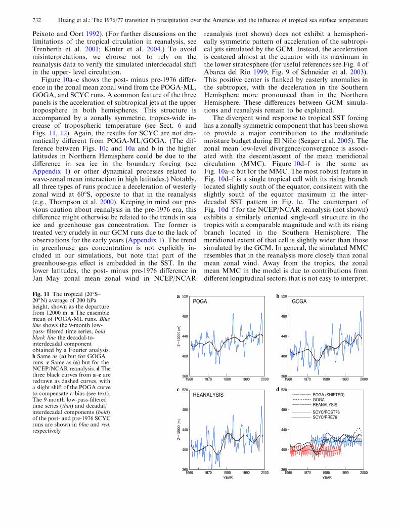
Before proceeding further, we should now verify thatthe POGA-ML, GOGA, and SCYC runs producecomparable interdecadal (upward) shifts in the tropics-wide tropospheric temperature across the 1976 transi-tion. The 200 hPa height averaged over the tropics(20�S–20�N) is used as an index for tropical tropospherictemperature. (The 200 hPa level is lifted when the tro-posphere expands due to an increased temperature.)Figure 11a–c shows this index, denoted as Z200, for1961–1998 from the POGA-ML and GOGA runs andthe NCEP/NCAR reanalysis. The thin blue lines are the9-month low-pass filtered time series of Z200, shown asits departure from 12,000 m, and bold black lines thedecadal-to-interdecadal component consisting of onlythe variability with T>6 years. Although the annualcycle is retained in the blue lines in Fig. 11a–c, it isoverwhelmed by interannual variability. For example,the four highest peaks in the blue line in Fig. 11a are dueto the 1982/83, 1986/87, 1992/93, and 1997/98 El Ninos.They contribute to the higher epoch mean of Z200 in thepost-1976 period. The decadal-to-interdecadal compo-nents in Fig. 11a–c are very similar, all showing an up-ward trend for the second half of the twentieth centurybut with the 1976 shift more pronounced in the reanal-ysis (see also Seager et al. 2004). The three black curvesin Fig. 11a–c are re-plotted in Fig. 11d as the dashedcurves. Because the Z200 for POGA-ML is systematicallyhigher than GOGA (by about 13 m, a small bias con-sidering that the total 200 hPa height is over 12,000 m),the POGA-ML case in Fig. 11d is shifted for the pur-pose of demonstration. All three dashed curves inFig. 11d show a clear elevation of Z200 in the post-1976era. Also shown in Fig. 11d are the post-1976 (blue) andpre-1976 (red) SCYC runs, presented in the same format

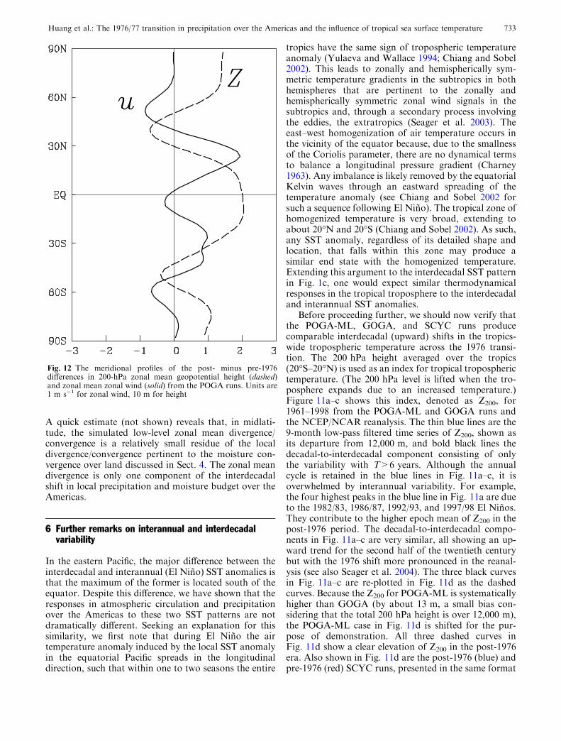
Fig. 12 The meridional profiles of the post- minus pre-1976differences in 200-hPa zonal mean geopotential height (dashed)and zonal mean zonal wind (solid) from the POGA runs. Units are1 m s�1 for zonal wind, 10 m for height


as Fig. 11a–c. The 9-month low-pass filtered time series(thin lines) for the SCYC runs are dominated by theannual cycle, with only weak and random interannualand decadal variability. Nevertheless, because the trop-ical mean SST is higher in the post-1976 period, it ele-vates the epoch mean of Z200 for this period, resulting ina post- minus pre-1976 difference in Z200 comparable tothose obtained from POGA-ML, GOGA, and reanaly-sis. The meridional profiles of the post- minus pre-1976zonal mean 200 hPa geopotential height and zonal windfor POGA-ML runs are shown in Fig. 12. The tropicalwarming zone extends to 20�–25� latitudes, where asharp meridional temperature (or height) gradient isaccompanied (noting thermal wind balance) by anenhanced subtropical jet in both hemispheres. Thestructure of the height anomaly in Fig. 12 is also remi-niscent of those associated with multi-year droughtsanalyzed by Schubert et al. (2004, see their Figs. 2, 6).

By a thermodynamical control argument (Chiangand Sobel 2002 and references therein), the uniformband of warmer tropical air in the post-1976 era couldinduce detailed structures in tropical precipitationanomalies common to the POGA-ML, GOGA, andSCYC runs. For example, as an El Nino or inter-decadal SST anomaly produces the banded warming inthe tropical troposphere, warmer air would spreadeastward over the Amazon, reducing the local lapserate there. This results in a more stable atmospherewith suppressed precipitation (as in Figs. 2, 3) andanomalous descent. The weaker upward motion is inturn compensated by a reduced low-level convergence(as in Figs. 6d, 7d). (The last two steps are our owninterpretation. Chiang and Sobel (2002) have focusedon the thermodynamical mechanism over the ocean.) Inthis view, the chain of reaction starts with the changein tropospheric temperature induced by remote SSTanomalies. The change in local low-level divergence orvertical motion is a passive response to the change inprecipitation, which itself is an adjustment to thechange in vertical thermodynamical profile. This argu-ment is appealing as it does not depend on the detail ofthe SST anomalies.

Note that the effect of an increased CO2 concentra-tion, which might be partially responsible for theobserved interdecadal changes in precipitation, isimplicitly embedded in the SST in our model (in thesense that an increase in the tropical Pacific SST issimulated by many coupled GCMs with double CO2, asmentioned in Sect. 2). Clearly, the trend in SST alonedoes not represent the complete effect of the greenhousegas forcing. If an explicit trend in CO2 were included inour simulations, land masses would have likely warmedup more dramatically in the last 40 years. In the contextof our thermodynamical argument, this would weakenthe expected effect of the stabilization of the troposphereover the Amazon (as suggested to the authors by E. K.Schneider). This might explain why the simulated dryingover the Amazon in Fig. 2c is more extensive than thatobserved in Fig. 2a.

For ENSO variability, although the zonal band oftropospheric warmth is restricted to the tropics, itsexistence is enough to induce a secondary response indynamical fields (Seager et al. 2003 and referencestherein) and precipitation (Seager et al. 2005) in theextratropics in both hemispheres. Details aside, in thisscenario the midlatitude response is controlled by thetropical tropospheric warmth. Thus, if the tropical warmbands produced by the interannual and interdecadalSST anomalies are similar, they would induce similarresponses in midlatitude. Robinson (2002) and Seageret al. (2003) suggest that the secondary extratropicalresponse is driven by the eddies that propagate differ-ently after the modification of the large-scale wind/temperature basic states by the tropical warmth. It isworth extending their analyses to interdecadal variabil-ity in the future.

In the tropics, some differences between the simulatedENSO and interdecadal precipitation anomalies remain(compare Fig. 2c to Fig. 3b) that cannot be explained bythe thermodynamical argument. Most notable in theAmerican sector is the dryness over the Caribbean andnorthern tip of South America in the interdecadal pat-tern that is absent in the ENSO composite for theGOGA runs. This could be the region where the directcirculation response to the detailed SST anomaliesmatters. To test this, one would need a dynamical modelfor the tropics that can predict the divergent windresponse to SST forcing (for example, the damped linearsolution of Gill (1980) or the inviscid nonlinear solutionof Schneider (1987), preferably modified to incorporatemore realistic orography and vertical resolution.) Therelative importance of the thermodynamical anddynamical control of SST-induced precipitation anom-alies needs further investigations.

While the similarity between the simulated precipi-tation in GOGA and POGA-ML runs indicates theimportance of tropical Pacific SSTs, it does not rule outpotential contributions of the Indian Ocean SST to theinterdecadal precipitation anomalies over the Americas.Because the SST anomalies in Indian and other oceanbasins are influenced by the tropical Pacific SST throughthe ‘‘atmospheric bridge’’ (Alexander et al. 2001), itmight be more difficult to isolate their effects withPOGA-ML type experiments. Within the Pacific basin,there are interesting features in the interdecadal SSTpatterns in Fig. 1, notably the hot (or cold) spot off thecoast of Mexico, which have not been emphasized in thiswork. As this hot spot is represented by a very smallnumber of grid points due to the moderate T42 resolu-tion of CCM3.10, simulations with a high-resolutionregional model may be more suitable for clarifying theimpact of this SST anomaly pattern on regional pre-cipitation.

The similarity between the precipitation in SCYC andGOGA/POGA-ML runs indicates that the rectifiedeffect of interannual variability is not crucial for pro-ducing the interdecadal shift in precipitation over theAmericas. This is understood in the sense that one does


not need to accumulate the responses in precipitation toindividual El Ninos/La Ninas in order to recover theinterdecadal anomalies in precipitation. In other words,the rectified effect arising from the nonlinear relation-ship between SST and midlatitude precipitation isunimportant. To the first order, the interdecadal pre-cipitation anomalies are linear responses to the inter-decadal modulation of tropical SSTs. The latter, whichis reflected in the difference between the post- and pre-1976 mean seasonal cycles of SST in the SCYC runs,could be due to the various causes—global warming,internal atmosphere–ocean dynamics, and changes inthe characteristics of El Nino—cited in the Introduction.Our conclusions are restricted to the precipitationresponses to given SSTs and do not endorse or reject anyof these scenarios regarding the origins of the inter-decadal SST patterns.

7 A 1998 reversal?

We have chosen the middle of 1998 as the end point ofthe post-1976 period, based on recent observations thatsuggest a reversal of the post-1976 trend in the pre-cipitation over several regions of the Americas, notablythe occurrence of the 1998-present North Americandrought (Hoerling and Kumar 2003). Comparing

Fig. 13a, the observed ‘‘post-1976 minus post-1998’’difference in the Jan–May precipitation, to the ‘‘post-1976 minus pre-1976’’ picture in Fig. 2a, one findssimilarities in the southwest U.S. and northern half ofSouth America but also differences elsewhere. (Here,the post-1998 period is defined as July 1998–June 2003.The NOAA/CPC CMAP data set, which incorporatedSatellite observations, is used for Fig. 13a. It was notused in Sect. 4 as it starts in 1979. Without 1976–1978in the CMAP data, the ‘‘post-1976’’ period shown inFig. 13 is actually ‘‘post-1978’’ but the minor differenceis inconsequential.) It is interesting to compare thesimulated changes in precipitation across the twoturning points at 1976 and 1998. For this purpose, asmaller set of 16 ensemble members of the GOGA runs(marked in Fig. 13 as ‘‘GOGA2’’) are extended to2004. The model reproduced the ‘‘post-1976 minuspost-1998’’ differences in precipitation over Mexico andthe southwest U.S. and the northern half of SouthAmerica, as shown in Fig. 13b. The Jan–May SSTanomaly, defined as the departure from the 1871–1999mean, for the post-1998 period is shown in Fig. 14. It isquite different from the pre-1976 picture in Fig. 2b.The equatorial Pacific has cooled but the rest of theIndo-Pacific Oceans remains warm. In addition, thecold anomaly is centered on the equator, in the middleof the basin. (Hoerling and Kumar 2003 suggest that

a

b

Fig. 13 The ‘‘post-1976 minuspost-1998’’ difference in theJan-May precipitation for aobservation based on theCMAP data set. b Ensemblemean of 16 GOGA runs. Colorscales are indicated at thebottom


this unique SST pattern is responsible for producingthe 1998–2002 North American drought.) With thislimited evidence, we suggest that the post-1976 ‘‘warmphase’’ (characterized by the SST pattern in Fig. 1a)has ended but a new ‘‘cold phase’’ of an interdecadaloscillation has not yet been fully established.

8 Conclusions

Most major features of the interdecadal shift in borealwinter–spring precipitation over the American conti-nents across the 1976 transition are reproduced inatmospheric GCM simulations forced with observedSST. The POGA-ML runs forced with specified tropi-cal Pacific SST produce similar results as the GOGAruns with global SST, indicating the importance oftropical Pacific SST in forcing interdecadal variabilityin precipitation over the Americas. Two types of sim-ulations with the forcing including (GOGA) andexcluding (SCYC) interannual variability of tropicalPacific SST also produce similar interdecadal shifts inthe upper-level circulation and precipitation over landin the American sector. This indicates that the precip-itation shifts arise fundamentally from shifts in themean tropical climate rather than as a rectified effectdue to the nonlinear relationship between SST andprecipitation. In fact, the observed and simulated in-terdecadal shifts in Jan–May precipitation—wet overMexico and the southwest U.S., dry over the Amazon,wet over sub-Amazonian South America, and dry overthe southern tip of South America—are not dramati-cally different from a typical El Nino-induced responsein precipitation. This implies that the responses inatmospheric circulation and precipitation over theAmericas are not sensitive to the detailed differencesbetween the El Nino and interdecadal SST anomalypatterns, the latter having its maximum south of theequator. The ‘‘tropospheric temperature’’ controlthinking (Chiang and Sobel 2002; Neelin et al. 2003),namely, warm tropical Pacific SST anomalies influenceremote precipitation by elevating and homogenizingtropics-wide tropospheric temperature, provides aplausible explanation of this insensitivity for the re-sponses in the tropics. The tropical troposphericwarmth common to the interannual and interdecadalatmospheric responses may, in turn, induce similarsecondary responses in the extratropics through an

anomalous eddy forcing as argued by Seager et al.(2003) and Robinson (2002).

An analysis of local moisture budget shows that,except for Mexico and the southwest U.S. where theincrease in precipitation after 1976 is balanced byevaporation, the shift in precipitation elsewhere over theAmerican continents is balanced by low-level moistureconvergence. Furthermore, the interdecadal shift inmoisture convergence is due mainly to the change inlow-level wind divergence that is linked to low-level as-cent and descent. This is similar to the finding of Seageret al. (2005) for ENSO variability that the tropical SST-forced wet precipitation anomalies in midlatitudes areassociated with anomalous ascent.

The two decades of dry tropics and wet midlatitudesover the Americas ended in 1998. The model resultsshow that this latest shift was caused by the shift tocooler SSTs in the tropical Pacific, even as the IndianOcean remained warm.

The findings in this study reinforce the emergingconsensus of the tropical control of global climate,previously explored in the context of multi-yeardroughts (Hoerling and Kumar 2003; Schubert et al.2004; Seager et al. 2005; manuscript submitted to J.Climate), hemispherically symmetric climate variability(Seager et al. 2003), and the long-term trend (Hoerlinget al. 2001; Schneider et al. 2003) in observations and/orGCM simulations.

Acknowledgements The authors thank Dr. Naomi Naik for valu-able help and advices on the models used in this study, Dr. AlexeyKaplan for providing up-to-date SST data sets for the GCMexperiments, and the two anonymous reviewers and Dr. EdwinSchneider for useful comments. The GFDL data used in Fig. 15awas provided by GFDL’s climate modelling group. This work issupported by the NOAA CLIVAR-PACS program and NSFgrant ATM 0347009, and is funded in part under the CooperativeInstitute for Climate Applications and Research (CICAR) awardnumber NA03OAR4320179 from the National Oceanic andAtmospheric Administration, U.S. Department of Commerce.This is Lamont-Doherty Earth Observatory Contribution No.6735.

Appendix 1

Models and SST for GCM experiments

The GOGA, POGA-ML, and SCYC runs were per-formed for multiple purposes and executed over time in

Fig. 14 The Jan–May SST anomaly, defined as the departure from the 1871–1999 mean, for the post-1998 period. Contour interval 0.1�C,negative dashed. Areas with the absolute value of SST anomaly greater than 0.1�C are filled with red (positive) and blue (negative) colors


conjunction with the ongoing updates of several com-prehensive SST data sets. As a result, they were notforced with exactly the same SST data set. This doesnot affect our conclusions, as the SST forcing for thepost-1961 period considered in this work does not de-pend strongly on the choice of the data set. Specifically,in the GOGA experiments the atmosphere GCM usesobserved SSTs in its lower boundary. These use a blendof data sets. The HadISST data set (Rayner et al. 2003)begins in 1870 and is global. The data set of Kaplanet al. (1998) begins in 1856, is not global, but doescontain data in the tropics for the whole time. There-fore, for the tropical Pacific (20�N–20�S) we use Kap-lan data from 1856 to 2001. From 1856 to 1870, andoutside of the tropical Pacific, we use Kaplan datawhere available and otherwise use climatological SSTsfrom HadISST. From 1870 on, and outside the tropicalPacific, we use the HadISST data. The SSTs weresmoothed linearly in latitude across a 10� wide beltbetween the tropical Pacific and the north and southPacific Oceans. This ensures that the merger does notproduce a jump discontinuity in space. A comparisonof our GOGA runs with a set of similar runs forcedwith a single set of SST forcing (see Fig. 15b) revealsminimal differences, inconsequential to our conclu-sions.

For the POGA-ML experiments, we only specify theSST in the tropical Pacific, using the Kaplan data, andcompute the SSTs everywhere else using an ocean mixedlayer model to be described shortly. In this model, SSTanomalies outside of the tropical Pacific can only begenerated by surface flux variability caused by internalatmospheric variability or forced as a response to theimposed tropical Pacific variability.

The epoch-mean seasonal cycles of SST used to forcethe SCYC runs are constructed from the HadISST1 dataset (Rayner et al. 2003). Due to the great uncertainty insea ice in the pre-1976 era, we choose not to include theepoch difference in sea ice in the boundary forcing. Adefault climatological annual cycle of sea-ice distribu-tion (constructed from 1979–1995) that came with theCCM3.10 model is used in both post- and pre-1976 runs.Thus, the difference between the two SCYC runs reflectsonly the impact of the open-ocean SST in the middle andlower latitudes.

In the POGA-ML runs, the atmospheric GCM iscoupled to a model of the ocean mixed layer (ML)outside the tropical Pacific. The ML model is basedon Russell et al. (1985) and includes a variable depthsurface layer that exchanges mass and heat with alayer below that extends down to a uniform specifieddepth. The depth of the surface layer follows a pre-

a

b

Fig. 15 a The post-1976 minuspre-1976 precipitationsimulated by a single GOGArun with the GFDL AM2model. b Same as a but for theensemble average of 12 GOGAruns with NCAR CCM3.6. Seetext for details


scribed seasonal cycle that is spatially variable andwhich follows the observed ML depth, taken to be thedepth where the temperature falls more than 0.5 Kcooler than the SST using the data of Levitus andBoyer (1994). The surface layer exchanges heat withthe atmosphere according to the atmosphere GCM’scomputation of the surface energy fluxes. The surfacelayer exchanges heat with the subsurface layer that isderived from the specified mass exchange and themodelled layer temperatures. The movement of heatby ocean currents in each layer is specified accordingthe the ‘‘q-flux’’ formulation: a spatially varying sea-sonal cycle of ‘‘q-flux’’ is diagnosed for each layer asthat which is required to maintain the observed cli-matological model temperatures when the ocean modelis coupled to the atmosphere GCM (see Russell et al.1985 for details). The q-fluxes also account forerrors in the modeled surface flux (and other modelerrors) but, primarily, account for the ocean heattransport.

The T42, 18-level version of NCAR CCM3.10 isadopted as the atmospheric GCM for our GOGA,POGA-ML, and SCYC experiments. Although ourresults are based on one model, preliminary model in-tercomparisons indicate that the multidecadal changein precipitation simulated by CCM3.10 (and verifiedwith observations) is not sensitive to the model and theSST data set used for boundary forcing. Figure 15ashows the ‘‘post-1976 minus pre-1976’’ precipitation (tobe compared with Fig. 2c) simulated by a singleGOGA run with GFDL AM2 model. The wet condi-tion over southwest U.S. and Mexico and dry condi-tion over northern South America are reproduced.Figure 15b is similar to Fig. 15a but is the average ofan ensemble of 12 GOGA runs with NCAR CCM3.6(a close relative of CCM3.10), identical to those used inHuang et al. (2003). Here, 5 of the 12 members areforced with the Climate Analysis Center (CAC) SSTdata set, the other 7 with the slightly different NationalMeteorological Center (NMC) data set. Both CAC andNMC data sets are forerunners of the Reynolds SSTdata set (Smith et al. 1996), different from the Kaplanand HadISST data used in our experiments. Yet, thesimulated interdecadal changes in precipitation over theAmericas are very similar, confirming the insensitivityof our results to SST data set. The similarity betweenFigs. 2c and 15b (the latter forced by a single SST dataset) also reassures us of the soundness of our approachof combining Kaplan and HadISST data in theboundary SST forcing.

Appendix 2

Statistical significance of the simulated post- minus pre-1976 difference in precipitation

The quantity of our interest is the difference betweenthe post- and pre-1976 epoch means of precipitation

simulated by the GCM. Denoting the two epoch meansof precipitation for the k-th ensemble member of theGCM runs as PPOST, k and PPRE,k, we are concerned

Fig. 16 The map at top panel repeats Fig. 2c but with boxes 1–4marking the regions where the statistical significance of the post-minus pre-1976 difference in Jan–May precipitation, {DPk}, will betested for the GOGA runs. Lower panels marked by 1–4 are thehistograms of {DPk} for the 48 ensemble members for thecorresponding boxes. Units are mm/day for the abscissa andnumbers of ensemble members for the ordinate. The bin widths forthe histograms are 0.05 mm/day for box 1 and 0.1 mm/day for theother three boxes


about the statistics of DPk ” PPOST,k�PPRE,k. In par-ticular, we wish to determine, given the number ofindependent samples (considered here as the number ofensemble members), whether the mean of {DPk} issignificantly positive or negative at the major centers ofthe pan-American precipitation pattern discussed in themain text. As a demonstration, the map in Fig. 16 re-peats the ensemble mean post- minus pre-1976 differ-ence in the simulated precipitation for the GOGA runsbut with boxes 1–4 added to indicate selected regionsfor a significance test. The histograms of area-averaged{DPk} for the 4 boxes for the 48 members of theGOGA runs are shown in the lower panels in Fig. 16.All ensemble members simulated a positive DPk for box1 (Mexico and part of the southwest U. S.) and anegative DPk for box 2 (northern South America), andall but one simulated a positive DPk for box 3 (middleSouth America). Combining the ensemble mean,0.24 mm/day, standard deviation, 0.086 mm/day, andthe number of independent samples, n=48, for box 1,one can immediately infer by Student’s t test (see e.g.,the rule of thumb, Eq. 1, in Sardeshmukh et al. 2000)that the post- minus pre-1976 difference in precipitationfor this box is greater than 0.2 mm/day at above 95%significance level. A similar test shows that the mean ofDPk is less than �0.52 mm/day for box 2 and greaterthan 0.23 mm/day for box 3, both at above 95% level.To provide a contrast, box 4 is chosen as a region witha small ensemble mean signal. Of the 48 members, 19(29) simulated a negative (positive) DPk. The ensemblemean, �0.004 mm/day, and standard deviation,0.166 mm/day, indicate that the 48 samples are notenough to establish that the mean of DPk is distin-guishable from 0 at 95% level.

Appendix 3

Decomposing the interdecadal shift in a quadratic term

Defining the interdecadal shift in a single variable Xacross the 1976 transition as dX ” [X]POST76

�[X]PRE76, we will derive an expression for the inter-decadal shift in a quadratic quantity, XY. For clarity,a bracket, [ ], is used in this appendix to indicate themean of the post- or pre-1976 epoch. By definition(subscripts ‘‘POST’’ and ‘‘PRE’’ stand for post- andpre-1976),

dðXYÞ ¼ ½XY �POST � ½XY �PRE: ð7Þ

For either the post- or pre-1976 period, the epochmean of XY can be written as

½XY � ¼ ½X �½Y � þ ½X �Y ��; ð8Þ

where X* is the year-to-year anomaly (departure fromthe epoch mean) of X due to interannual variability.Combining Eqs. 7 and 8, one obtains

dðXY Þ ¼ ½X �POST½Y �POST þ ½X � Y ��POST

�½X �PRE½Y �PRE � ½X � Y ��PRE

¼ ½X �PRE þ dX� �

½Y �PRE þ dY� �

þ½X � Y ��POST � ½X �PRE½Y �PRE

�½X � Y ��PRE

¼ ðdY Þ½X �PRE þ ðdX Þ½Y �PRE

þdXdY þ ½X � Y ��POST

�½X � Y ��PRE: ð9Þ

Reverting to the notation in Eq. 6, [X]PRE and [Y]PRE

are XC and YC. The last three terms in the r.h.s. ofEq. (9) are the ‘‘higher-order terms’’. The dXdY term issmaller than the first two terms in the r.h.s. of Eq. (9) if|XC| >> |dX|, |YC| >> |dY|, which is generally truefor horizontal velocity and specific humidity. The lasttwo terms in Eq. 9 indicate that the difference betweenthe interannual variability in the post- and pre-1976periods could contribute to the difference in the epochmeans (of a quadratic quantity) of the two periods. Thiscontribution might not be negligible in the POGA-MLand GOGA runs and in observations, due to the pres-ence of more strong El Nino events in the post-1976 era.By design, however, it is small for the SCYC runs con-sidered in Sect. 4, since the ‘‘repeated seasonal cycle’’experiments produce only weak and random interannualvariability (see Fig. 11d). Thus, for the analyses in Sect.4 for the SCYC runs, the last three terms in Eq. 9 areneglected as the higher-order terms. This is justified aposteriori as the sum of the four retained terms in Eq. 6turns out to be very close to the total (compare Figs. 6eand 4c).

References

Abarca del Rio R (1999) The influence of global warming in Earthrotation speed. Ann Geophys 17:806–811

Alexander MA, Blade I, Newman M, Lanzante JR, Lau NC, ScottJD (2001) The atmospheric bridge: the influence of ENSO tel-econenctions on air-sea interaction over the global oceans.J Climate 15:2205–2231

Allan RP, Slingo A, Ramaswamy V (2002) Analysis of moisturevariability in the European Centre for Medium-Range Fore-casts 15-year reanalysis over the tropical oceans. J Geophys Res107:4230, 10.1029/2001JD001132

Bates GT, Hoerling MP, Kumar A (2001) Central U.S. springtimeprecipitation extremes: teleconnections and relationship withsea surface temperature. J Climate 14:3751–3766

Boer GJ, Yu B, Kim SJ, Flato GM (2004) Is there observationalsupport for an El Nino-like pattern of future global warm-ing? Geophys Res Lett 31: L06201, doi:10.1029/2003GL018722

Cane MA, Clement AC, Kaplan A, Kushnir Y, Murtugude R,Pozdnyakov D, Seager R, Zebiak SE (1997) Twentieth centurysea surface temperature trends. Science 275:957–960

Cayan DR, Dettinger MD, Diaz HF, Graham NE (1998) Decadalvariability of precipitation over western North America. J Cli-mate 11:3148–3166


Charney JG (1963) A note on large-scale motions in the tropics.J Atmos Sci 20:607–609

Chiang JCH, Sobel AH (2002) Tropical tropospheric temperaturevariations caused by ENSO and their influence on the remotetropical climate. J Climate 15:2616–2631

Chou C, Neelin JD (2004) Mechanisms of global warming impactson regional tropical precipitation. J Climate 17:2688–2701

Deser C, Phillips AS, Hurrell JW (2004) Pacific interdecadal cli-mate variability: linkages between the Tropics and North Pa-cific during boreal winter since 1900. J Climate 17:3109–3124

Fedorov AV, Philander SG (2001) A stability analysis of tropicalocean-atmosphere interaction: bridging measurements andtheory for El Nino. J Climate 14:3086–3101

Giannini A, Saravanan R, Chang P (2004) The preconditioningrole of tropical Atlantic variability in the development of theENSO teleconnection: implications for the prediction ofNordeste rainfall. Clim Dyn 22:839–855

Gill AE (1980) Some simple solutions for the heat-induced tropicalcirculation. Q J R Meteor Soc 106:447–462

Goddard L, Mason SJ, Zebiak SE, Ropelewski CF, Basher R,Cane MA (2001) Current approaches to seasonal-to-interan-nual climate predictions. Int J Climatol 21:1111–1152

Gu DF, Philander SGH (1997) Interdecadal climate fluctuationsthat depend on exchanges between the tropics and extratropics.Science 275:805–807

Hoerling MP, Kumar A (2003) The perfect ocean for drought.Science 299:691–694

Hoerling MP, Hurrell JW, Xu T (2001) Tropical origins for recentNorth Atlantic climate change. Science 292:90–92

Hsu HH, Lin SH (1992) Global teleconnections in the 250-mbstreamfunction field during the Northern Hemisphere winter.Mon Weather Rev 120:1169–1192

Huang HP, Weickmann KM, Hsu CJ (2001) Trend in atmosphericangularmomentum in a transient climate change simulationwithgreenhouse gas and aerosol forcing. J Climate 14:1525–1534

Huang HP, Weickmann KM, Rosen RD (2003) Unusual behaviorin atmospheric angular momentum during the 1965 and 1972 ElNino. J Climate 16:2526–2539

Kaplan A, Cane M, Kushnir Y, Clement A, Blumenthal M, Raj-agopalan B (1998) Analyses of global sea surface temperature1856–1991. J Geophys Res 103:18567–18589

Karspeck AR, Seager R, Cane MA (2004) Predictability of tropicalPacific decadal variability in an intermediate model. J Climate17:2842–2850

Kinter III JL, Fennessy MJ, Krishnamurthy V, Marx L (2004) Anevaluation of the apparent interdecadal shift in the tropicaldivergent circulation in the NCEP-NCAR reanalysis. J Climate17:349–361

Knutson TR, Manabe S (1995) Time-mean response over thetropical Pacific to increased CO2 in a coupled ocean-atmo-sphere model. J Climate 8:2181–2199

Kumar A, Yang F, Goddard L, Schubert S (2004) Differing trendsin the tropical surface temperatures and precipitation over landand oceans. J Climate 17:653–664

Lau NC, Leetmaa A, Nath MJ, Wang HL (2005) Influences ofENSO-induced Indo-Western Pacific SST anomalies on extra-tropical atmospheric variability during the boreal summer.J Climate (in press)

Levitus SE, Boyer T (1994) World ocean atlas 1994, vol 4: tem-perature, NOAA Atlas NESDIS 4, U. S. Department ofCommerce, Washington

McPhaden MJ, Zhang D (2002) Slowdown of the meridionaloverturning circulation in the upper Pacific Ocean. Nature415:603–608

Nakamura H (1993) Horizontal divergence associated with zonallyisolated jet streams. J Atmos Sci 50:2310–2313

Neelin JD, Chou C, Su H (2003) Tropical drought regions in globalwarming and El Nino teleconnections. Geophys Res Lett30:doi:10.1029/2003GLO018625

Peixoto JP, Oort AH (1992) Physics of climate. American Instituteof Physics, New York, p 520

Qin J, Robinson WA (1993) On the Rossby wave source and thesteady linear response to tropical forcing. J Atmos Sci 50:1819–1823

Rayner NA, Parker DE, Horton EB, Folland CK, Alexander LV,Rowell DP, Kent EC, Kaplan A (2003) Global analyses of seasurface temperature, sea ice, and night marine air temperaturesince the late nineteenth century. J Geophys Res 108:Art. No.4407

Robinson WA (1994) Comments on ‘‘Horizontal divergence asso-ciated with zonally isolated jet streams’’. J Atmos Sci 51:1760–1761

Robinson WA (2002) On the midlatitude thermal response totropical warmth. Geophys Res Lett 29:doi:10.1029/2001GL014158

Ropelewski CF, Halpert MS (1987) Global and regional scaleprecipitation patterns associated with the Southern Oscillation.Mon Weather Rev 115:1606–1626

Russell GL, Miller JR, Tsang LC (1985) Seasonal oceanic heattransports computed from an atmospheric model. Dyn AtmosOceans 9:253–271

Sardeshmukh PD, Hoskins BJ (1988) The generation of globalrotational flow by steady idealized tropical divergence. J AtmosSci 45:1228–1251

Sardeshmukh PD, Compo GP, Penland C (2000) Changes ofprobability associated with El Nino. J Climate 13:4268–4286

Schneider EK (1987) A simplified model of the modified Hadleycirculation. J Atmos Sci 44:3311–3328

Schneider EK, Bengtsson L, Hu ZZ (2003) Forcing of NorthernHemisphere climate trends. J Atmos Sci 60:1504–1521

Schubert SD, Suarez MJ, Pegion PJ, Koster RD, Bacmeister JT(2004) Causes of long-term drought in the United States GreatPlains. J Climate 17:485–503

Seager R, Harnik N, Kushnir Y, Robinson W, Miller J (2003)Mechanisms of hemispherically symmetric climate variability.J Climate 16:2960–2978

Seager R, Karspeck A, Cane M, Kushnir Y, Giannini A, KaplanA, Kerman B, Miller J (2004) Predicting Pacific decadal vari-ability. In: Wang C, Xie S-P, Carton J (eds) Earth Climate: TheOcean-Atmosphere Interaction. American Geophysical Union,Washington, pp 105–120

Seager R, Harnik N, Robinson WA, Kushnir Y, Ting M, HuangHP, Velez J (2005) Mechanisms of ENSO-forcing of hemi-spherically symmetric precipitation variability. Q J R MeteorolSoc (in press)

Smith TM, Reynolds RW, Livezey RE, Stokes DC (1996) Recon-struction of historical sea surface temperatures using empiricalorthogonal functions. J Climate 9:1403–1420

Thompson DWJ, Wallace JM, Hegerl GC (2000) Annular modes inthe Extratropical circulation, part II: trends. J Climate 13:1018–1036

Trenberth KE (1990) Recent observed interdecadal climatechanges in the Northern Hemisphere. Bull Amer Meteor Soc71:988–993

Trenberth KE, Branstator GW, Karoly D, Kumar A, Lau NC,Ropelewski C (1998) Progress during TOGA in understandingand modeling global teleconnections associated with tropicalsea surface temperature. J Geophys Res 103:14291–14324

Trenberth KE, Stepaniak DP, Hurrell JW, Fiorino M (2001)Quality of reanalysis in the tropics. J Climate 14:1499–1510

Webster PJ, Holton JR (1982) Cross equatorial response to middle-latitude forcing in a zonally varying basic state. J Atmos Sci39:722–733

Yulaeva E, Wallace JM (1994) The signature of ENSO in globaltemperature and precipitation fields derived from the micro-wave sounding unit. J Climate 7:1719–1736


Æ the 1976/77 transition in precipitation over the...

Documents