a techno-economic & environmental analysis of a novel
TRANSCRIPT

A techno-economic & environmental analysis of a novel technology
utilizing an internal combustion engine as a compact, inexpensive
micro-reformer for a distributed gas-to-liquids system
Joshua B. Browne
Submitted in partial fulfillment of the
requirements for the degree of
Doctor of Philosophy
in the Graduate School of Arts and Sciences
COLUMBIA UNIVERSITY
2016

© 2016
Joshua B. Browne
All rights reserved

ABSTRACT
“A techno-economic & environmental analysis of a novel technology
utilizing an internal combustion engine as a compact, inexpensive
micro-reformer for a distributed gas-to-liquids system”
Joshua B. Browne
Anthropogenic greenhouse gas emissions (GHG) contribute to global warming, and must be
mitigated. With GHG mitigation as an overarching goal, this research aims to study the potential
for newfound and abundant sources of natural gas to play a role as part of a GHG mitigation
strategy. However, recent work suggests that methane leakage in the current natural gas system
may inhibit end-use natural gas as a robust mitigation strategy, but that natural gas as a feedstock
for other forms of energy, such as electricity generation or liquid fuels, may support natural-gas
based mitigation efforts.1
Flaring of uneconomic natural gas, or outright loss of natural gas to the atmosphere results in
greenhouse gas emissions that could be avoided and which today are very large in aggregate. A
central part of this study is to look at a new technology for converting natural gas into methanol
at a unit scale that is matched to the size of individual natural gas wells. The goal is to convert
stranded or otherwise flared natural gas into a commercially valuable product and thereby avoid
any unnecessary emission to the atmosphere.
1 While it is generally understood that fuel switching from coal to natural gas in the electricity sector reduces GHG
emissions, it should be noted that the mitigation potential of natural gas use in the electricity sector is influenced by
the methane leakage between the well and the power plant, thus bringing into question the overall GHG reduction
potential in light of current leakage percentage uncertainty.

A major part of this study is to contribute to the development of a novel approach for converting
natural gas into methanol and to assess the environmental impact (for better or for worse) of this
new technology. This Ph. D. research contributes to the development of such a system and
provides a comprehensive techno-economic and environmental assessment of this technology.
Recognizing the distributed nature of methane leakage associated with the natural gas system,
this work is also intended to advance previous research at the Lenfest Center for Sustainable
Energy that aims to show that small, modular energy systems can be made economic. This thesis
contributes to and analyzes the development of a small-scale gas-to-liquids (GTL) system aimed
at addressing flared natural gas from gas and oil wells. This thesis includes system engineering
around a design that converts natural gas to synthesis gas (syngas) in a reciprocating internal
combustion engine and then converts the syngas into methanol in a small-scale reactor.
With methanol as the product, this research aims to show that such a system can not only address
current and future natural gas flaring regulation, but eventually can compete economically with
historically large-scale, centralized methanol production infrastructure. If successful, such
systems could contribute to a shift away from large, multi-billion dollar capital cost chemical
plants towards smaller systems with shorter lifetimes that may decrease the time to transition to
more sustainable forms of energy and chemical conversion technologies.
This research also quantifies the potential for such a system to contribute to mitigating GHG
emissions, not only by addressing flared gas in the near-term, but also supporting future natural
gas infrastructure ideas that may help to redefine the way the current natural gas pipeline system

is used. The introduction of new, small-scale, distributed energy and chemical conversion
systems located closer to the point of extraction may contribute to reducing methane leakage
throughout the natural gas distribution system by reducing the reliance and risks associated with
the aging natural gas pipeline infrastructure.
The outcome of this thesis will result in several areas for future work. From an economic
perspective, factors that contribute to overall system cost, such as operation and maintenance
(O&M) and capital cost multiplier (referred to as the Lang Factor for large-scale petro-chemical
plants), are not yet known for novel systems such as the technology presented here. From a
technical perspective, commercialization of small-scale, distributed chemical conversion systems
may create a demand for economical compression and air-separation technologies at this scale
that do not currently exist. Further, new business cases may arise aimed at utilizing small,
remote sources of methane, such as biogas from agricultural and municipal waste. Finally, while
methanol was selected as the end-product for this thesis, future applications of this technology
may consider methane conversion to hydrogen, ammonia, and ethylene for example, challenging
the orthodoxy in the chemical industry that “bigger is better.”

i
Table of Contents
List of Figures.. ............................................................................................................................. iv
List of Tables ................................................................................................................................ vi
CHAPTER 1: Motivation .............................................................................................................. 1
1.1 Mitigating anthropogenic greenhouse gas emissions ..................................................... 3
1.2 The natural gas system .................................................................................................... 4
1.2.1 Background ............................................................................................................... 4
1.2.2 Methane leakage ....................................................................................................... 6
1.3 Natural Gas Flaring: A distributed problem in need of a distributed solution ............. 10
1.4 System scale .................................................................................................................. 13
1.4.1 Small-scale gas-to-liquid development ......................................................................... 13
1.4.2 Micro-GTL system........................................................................................................ 15
CHAPTER 2: Engine Reformer – Technical Background .......................................................... 17
2.1 Integrated System Overview ......................................................................................... 17
2.2 Internal Combustion Engine Reformer ......................................................................... 20
2.2.1 Background ............................................................................................................. 20
2.2.2 Summary of Laboratory Scale Engine Testing ....................................................... 21
2.2.2.1 Syngas Production ........................................................................................... 21
2.2.2.2 Soot Formation ................................................................................................ 25
2.2.2.3 Sensitivity to Compression Ratio .................................................................... 27
CHAPTER 3: Integrated System - Aspen HYSYS Model .......................................................... 29
3.1 System Overview .......................................................................................................... 29
3.1.1 Inlet Feed Gas, Mixing, Boost, and Pre-heat .......................................................... 32
3.1.2 Engine Reformer ..................................................................................................... 34
3.1.2.1 Overview of Aspen Engine Reformer System ................................................ 34
3.1.2.2 Aspen Engine Reformer Model Steps ............................................................. 37
3.1.2.3 Aspen Engine Reformer Reactions.................................................................. 40

ii
3.1.2.4 Aspen Engine Reformer Exhaust Heat Utilization and Liquid Drop-out ........ 43
3.1.3 Syngas Compression ............................................................................................... 46
3.1.4 Methanol Reactor .................................................................................................... 49
3.1.4.1 Methanol Reactor – Thermodynamic Equilibrium Analysis ........................... 52
3.1.5 System Energy Budget ............................................................................................ 58
CHAPTER 4: Integrated System - Economic Analysis ............................................................... 62
4.1 Estimating Engine Cost................................................................................................. 62
4.2 Estimating System Engine Displacement ..................................................................... 68
4.3 System Capital Cost ...................................................................................................... 70
4.3.1 Capital Cost Multiplier ........................................................................................... 70
4.3.2 Syngas Production Step .......................................................................................... 73
4.3.3 Pre-conditioning Step incl. Compressor ................................................................. 74
4.3.4 Methanol Production - Reactor System Capital Cost ............................................. 76
4.3.5 Capital Cost with 95% O2 ....................................................................................... 77
4.4 Methanol Production Cost ............................................................................................ 79
4.4.1 Methodology ........................................................................................................... 79
4.4.2 System Specifications ............................................................................................. 81
4.4.3 Operation and Maintenance (O&M) ....................................................................... 83
4.4.4 Results ..................................................................................................................... 86
4.4.5 Sensitivity Analysis ................................................................................................ 91
CHAPTER 5: Syngas Production - Economic Analysis ............................................................. 96
5.1 Introduction ................................................................................................................... 96
5.2 Background ................................................................................................................... 97
5.3 Large-scale Syngas Production Cost Baseline .............................................................. 98
5.3.1 Large-scale Syngas Production Cost Calculations ............................................... 102
5.3.1.1 “Design and economics of a Fischer-Tropsch plant for converting natural gas
to liquid transportation fuels,” (Choi et al., 1997) ........................................................... 103
5.3.1.2 “Cost comparison of syngas production from natural gas conversion and
underground coal gasification,” (Pei et al., 2014) ........................................................... 108
5.3.1.3 “Optimization and selection of reforming approaches for syngas generation
from natural/shale gas.” (Noureldin et al., 2014) ............................................................. 112

iii
5.3.1.4 “Analysis of Natural Gas-to Liquid Transportation Fuels via Fischer-Tropsch.”
(National Energy Technology Laboratory, 2013) ............................................................ 114
5.4 Small-scale Syngas Production Cost Estimate ........................................................... 118
5.4.1 Integrated System Overview ................................................................................. 118
5.4.2 Engine Reformer Syngas Production Cost ........................................................... 119
5.5 Sensitivity Study ......................................................................................................... 124
5.5.1 Note on the cost basis used in this study............................................................... 126
CHAPTER 6: Life Cycle Analysis ............................................................................................ 128
6.1 Overview ..................................................................................................................... 128
6.2 Method ........................................................................................................................ 128
6.3 Results - Summary ...................................................................................................... 133
6.3.1 A Note on Global Warming Potentials ................................................................. 134
6.4 Results – Sensitivity Studies ....................................................................................... 135
6.4.1 Methane Leakage Rates ........................................................................................ 135
6.4.2 Methanol transport from Heavy-Duty (HD) trucking ........................................... 137
6.4.3 Small-Scale GTL Conversion Efficiency ............................................................. 138
6.4.4 Engine reformer replacement ................................................................................ 140
CHAPTER 7: Discussion and Future Work .............................................................................. 142
Bibliography ............................................................................................................................... 148
Appendix A ................................................................................................................................. 153
Preliminary Case Study ........................................................................................................... 153
Overview ................................................................................................................................. 153
Background on associated gas characteristics in the Bakken field ......................................... 155
Business & Economic Model .................................................................................................. 156
Preliminary Sensitivity Analysis ............................................................................................. 160
Current Market Conditions ...................................................................................................... 162
Appendix B ................................................................................................................................. 164

iv
List of Figures
Figure 1: Natural Gas & Oil Spot Prices ....................................................................................... 4
Figure 2: Drilling Productivity Report, year-over-year summary ................................................. 5
Figure 3: Estimates of Natural Gas Emissions by Sub-Sector of Natural Gas System ................. 7
Figure 4: Marcellus Shale Gas Well Map (2004 – 2013) ............................................................ 12
Figure 5: Haynesville Shale Gas Well Activity Map................................................................... 13
Figure 6: Distribution of oil wells by volume of gas flared in the Bakken region ...................... 16
Figure 7: Average associated gas production in U.S. tight oil fields ........................................... 16
Figure 8: Possible commercial configuration of miniGTL system .............................................. 19
Figure 9: Possible uses for Syngas............................................................................................... 19
Figure 10: H2:CO ratio vs. Equivalency ratio, Φ. ....................................................................... 24
Figure 11: Mole Fraction of Exhaust Gas for a range of Equivalence Ratios (Φ) ...................... 25
Figure 12: Soot Concentration vs. Equivalency ratio, Φ ............................................................. 27
Figure 13: Simple block flow diagram ........................................................................................ 30
Figure 14: Aspen HYSYS process flow diagram ........................................................................ 30
Figure 15: Inlet feed, mixing, boost, and pre-heat ....................................................................... 33
Figure 16: Engine Reformer System ............................................................................................ 36
Figure 17: Engine reformer – power & reaction stroke ............................................................... 39
Figure 18: Reaction coefficients for engine reformer combustion/reaction stroke ..................... 42
Figure 19: Engine Reformer – Exhaust heat recycle loop ........................................................... 44
Figure 20: ‘SynGas’ feed and water separation ........................................................................... 47
Figure 21: 2-stage compression w/intercooling ........................................................................... 48
Figure 22: Methanol reactor (black box) ..................................................................................... 50

v
Figure 23: Methanol reactor example reaction coefficients ........................................................ 52
Figure 24: Simple Gibbs Reactor in Aspen Plus V8.6................................................................. 53
Figure 25: Temperature vs. Mole Fraction, baseline case ........................................................... 54
Figure 26: Pressure vs. Mole Fraction, baseline case .................................................................. 55
Figure 27: Temperature & Pressure vs. Methanol Production, baseline case ............................. 55
Figure 28: Temperature vs. Mole Fraction, 95% O2 case ............................................................ 57
Figure 29: Pressure vs. Mole Fraction, 95% O2 case ................................................................... 58
Figure 30: Per Liter Engine Production Cost vs. Engine Displacement ...................................... 67
Figure 31: Economic Analysis Methodology .............................................................................. 87
Figure 32: Methanol Production Cost Sensitivity (Tornado Chart) ............................................. 92
Figure 33: Process Flow Diagram for 50,000 bbl/day F-T system ............................................ 102
Figure 34: Block Diagram for Engine Reformer (Small-Scale) GTL System ........................... 118
Figure 35: Aspen Process Flow Diagram .................................................................................. 119
Figure 36: Syngas Production Cost Comparison ....................................................................... 124
Figure 37: Syngas Production Cost Sensitivity Study for Engine Reformer System ................ 126
Figure 38: Producer Price Index - Processed Fuels for Intermediate Demand .......................... 127
Figure 39: Process Map for large-scale, central methanol production (baseline) ...................... 131
Figure 40: Process Map for small-scale, on-site methanol production ...................................... 131
Figure 41: Service Provider Model ............................................................................................ 156
Figure 42: Per-year NPV for the MicroGTL System Lifetime .................................................. 160
Figure 43: Service Provider Model Sensitivity Analysis ........................................................... 161
Figure 44: Per-year NPV for Alternate Scenario using 2015 Average Prices ........................... 163
Figure 45: Per-year NPV for Alternate Scenario using Dec. 2015 Average Prices .................. 163

vi
List of Tables
Table 1: Stream table summary - inlet feed, mixing, boost, and pre-heat ................................... 34
Table 2: Stream table summary, engine reformer system ............................................................ 37
Table 3: Volumetric ratio values used for Aspen Engine Reformer model ................................. 40
Table 4: Stream table summary, exhaust system heat utilization and liquid drop-out ................ 44
Table 5: Stream table summary, syngas compression ................................................................. 48
Table 6: Stream table summary, methanol reactor – part 1 ......................................................... 51
Table 7: Stream table summary, methanol reactor – part 2 ......................................................... 51
Table 8: Component power & heat inputs and outputs from integrated system Aspen model ... 59
Table 9: Vehicle Manufacturing and Retailing Cost Structure .................................................... 64
Table 10: Vehicle Production Cost Allocation ............................................................................ 64
Table 11: Compiled engine cost data ........................................................................................... 66
Table 12: Input Variables for Engine Displacement Calculation ................................................ 69
Table 13: System Capital Cost ..................................................................................................... 73
Table 14: Methanol Production Cost Calculations ...................................................................... 80
Table 15: Summary of NPV Calculations ................................................................................... 90
Table 16: Methanol Production Cost ........................................................................................... 90
Table 17: Baseline Large-Scale System economic parameters ................................................. 100
Table 18: Economic factors for Choi, et al. ............................................................................... 105
Table 19: Economic Analysis Calculations for Choi, et al. ....................................................... 106
Table 20: NPV Calculations for Choi, et al. .............................................................................. 107
Table 21: GTL Plant Assumptions for Pei et al. ........................................................................ 109
Table 22: Syngas Production Cost vs. Natural Gas Price for Pei et al. ..................................... 110

vii
Table 23: NPV Calculations for Pei, et al. ................................................................................. 111
Table 24: H2:CO Ratio vs. Syngas Price for Noureldin, et al. ................................................. 113
Table 25: Syngas cost for H2:CO = 2.0 for Noureldin, et al. ..................................................... 113
Table 26: System Economic Factors for NETL F-T system..................................................... 116
Table 27: NPV Calculations for NETL F-T System .................................................................. 117
Table 28: Baseline Syngas Production Cost, 2014$/MMBtu .................................................... 118
Table 29: System Economic Factors for Engine Reformer System .......................................... 122
Table 30: NPV Calculations for Small-Scale Engine Reformer System ................................... 123
Table 31: Data for Syngas Production Cost Sensitivity Study .................................................. 126
Table 32: List of adjustments to GREET (version 2014) Excel-based model ........................... 130
Table 33: Life-Cycle Analysis Results for Baseline Large-Scale & MicroGTL Systems ........ 133
Table 34: Natural Gas System Methane Leakage Sensitivity Results ....................................... 137
Table 35: Results from HD trucking distance sensitivity study ................................................ 138
Table 36: Results from Conversion Efficiency Sensitivity Study ............................................. 139
Table 37: Engine Manufacturing Emissions .............................................................................. 140
Table 38: Economic Model Inputs and NPV result ................................................................... 159
Table 39: Range of Values for Sensitivity Study....................................................................... 161
Table 40: Methanol and Propane Spot Prices for Different Time Periods ................................ 162
Table 41: Material properties for stream flows included in Aspen Engine Reformer model .... 164

viii
Acknowledgements
First and foremost, I would like to thank my thesis adviser, Professor Klaus Lackner. Anyone
fortunate enough to spend time with Klaus knows how truly special he is both as an academic
adviser and as a person. Klaus’s guidance and mentorship throughout my doctoral studies were
invaluable, and his unwavering patience is without equal.
I would next like to thank my many colleagues at the Lenfest Center for Sustainable Energy.
Specifically, I would like to acknowledge:
Eric Dahlgren: Eric’s doctoral thesis provided the foundation for my thesis. I am
grateful for Eric’s guidance as I navigated through the Ph. D. process.
Zara L’Heureux: Zara taught me how to use Aspen, and she significantly contributed to
the work contained in this thesis.
Diego Villarreal: Diego and I met during orientation in Fall 2010 during the Climate and
Society Master’s Degree program orientation and we have been partners in crime ever
since. I have continually relied on Diego’s background in Chemical Engineering
throughout this thesis.
This thesis was part of a large collaboration between Columbia University, Massachusetts
Institute of Technology, and Research Triangle Institute International. MIT provided the initial
proof of concept work on the engine reformer system and has been a valuable collaborator.
From MIT, I would specifically like to thank:

ix
Dr. Leslie Bromberg: Leslie’s research formed the basis for this thesis. Leslie has been a
continued supporter throughout this project, and I look forward to collaborating with him
in the future.
Emmanuel Lim and Angi Acocella: Emmanuel and Angi were instrumental in the early
lab work at MIT. Emmanuel managed the engine testing at MIT, and graciously allowed
me to participate in this valuable work.
The rest of the talented group of professors and students at the MIT Sloan Auto Lab.
From RTI, I would like to acknowledge:
Vikram Rao: Vik is responsible for making the connection between MIT, RTI, and
Columbia and has provided industry expertise (and humor) throughout this thesis.
Raghubir Gupta: Raghubir served on my thesis committee and provided critical feedback
on my thesis. Raghubir has been a valuable mentor throughout this thesis, and has
become a close friend.
John Carpenter: John managed the larger collaborative effort between Columbia, MIT,
and RTI. John has been my gracious host during my many trips to RTI, and he has
patiently provided direction and guidance throughout this thesis.
Last, and certainly not least, I would like to thank my wife, Michelle, for supporting me on this
five year vacation from the real world. And of course, Tess.
____________

x
Financial support for this thesis was provided through the Department of Earth & Environmental
Engineering at Columbia University, and through a grant (Award #: DE-AR0000506) from the
U.S. Department of Energy’s Advanced Research Projects Agency – Energy (ARPA-E).

CHAPTER 1: Motivation
1
CHAPTER 1: Motivation
The work in this thesis is motivated by reducing the environmental footprint of a newly
developing energy infrastructure that is the result of the recent advancement in unconventional
natural gas and oil extraction from shale formations (a.k.a. hydraulic fracturing, or fracking).
Fracking and horizontal drilling has given access to vast natural gas and oil resources which until
recently were entirely out of reach of economic development. As a result, far more natural gas
has entered the U.S. market. Environmental concerns have been raised, because methane is a far
more potent greenhouse gas than carbon dioxide, and therefore leakage of methane from a
rapidly growing natural gas based energy infrastructure is becoming a serious concern.2 The
question arises: should natural gas be delivered to the end consumer, or would it be
advantageous to convert it into useful products closer to the point of extraction? It appears that
natural gas use in centralized electricity production reduces natural gas emissions (see footnote
#1). Based on average power plant heat rates, natural gas fired power plants emit approximately
half the CO2 emissions as coal fired power plants on a per-MWh basis (Rubin, Chen, & Rao,
2007; U.S. Energy Information Administration, 2016). Delivery of natural gas to the industrial
(i.e. liquid fuels production) or residential (space heating) end consumer, however, could have
unintended greenhouse gas implications that need to be explored further.
2 The Intergovernmental Panel on Climate Change (IPCC) Fifth Assessment Report (AR5) defines the Global
Warming Potential (GWP) for methane at 34 (34 times the radiative forcing of CO2) over a 100 year time horizon,
and 86 for a 20 year time horizon, including climate-carbon feedbacks (Myhre et al., 2013).

CHAPTER 1: Motivation
2
In addition, fracking has greatly increased the volumes of stranded natural gas. Natural gas that
cannot be economically delivered to the market is considered stranded. Natural gas produced
during the development of a new gas well is typically stranded due to the lack of a pipeline
infrastructure. Natural gas produced as a by-product of oil production, for example in the
Bakken Field in North Dakota, is very often uneconomic to recover and thus flared (typically
referred to as associated gas). This work is also motivated by the observation that in order to
render stranded gas economic, one must be able to operate conversion technology at scales small
enough to match the size of the source. Ideally the system required should be mobile, as a
particular natural gas well is not only small, but is also often short-lived. This observation has
connected this work to another area of research at the Lenfest Center which aims to show that
small, modular, mass-produced system could in the future compete with the large units that have
been deployed in the past. For them to become economical, they must be mass-produced,
require minimum maintenance and operate autonomously in a fully automated fashion
(Dahlgren, Göçmen, Lackner, & van Ryzin, 2013; Dahlgren, 2014).
A recent ARPA-E project that supports this thesis work brings together these various motivations
in a project that aims to demonstrate a technology that converts natural gas into syngas in a
modified reciprocating internal combustion engine, the syngas in turn is converted into methanol
in a small catalytic reactor.3,4
This thesis contributes to this effort, analyzes the environmental
footprint and economic viability of this new technology, and raises a number of important
3 ARPA-E: Advanced Research Projects Agency – Energy, U.S. Department of Energy
4 “Compact, inexpensive micro-reformers for distributed GTL,” DOE/ARPA-E Award #: DE-AR0000506

CHAPTER 1: Motivation
3
questions to further develop and refine this approach for radical transformation of our current
chemical manufacturing infrastructure.
1.1 Mitigating anthropogenic greenhouse gas emissions
The greenhouse effect and the influence of atmospheric greenhouse gasses on temperature have
been generally well understood for over 100 years (Arrhenius, 1896). The motivation for
mitigating greenhouse gas emissions from fossil fuel burning is succinctly summarized in the
most recent IPCC fifth Assessment Report with the following statements (IPCC et al., 2013) :
“Warming of the climate system is unequivocal, and since the 1950s, many of the
observed changes are unprecedented over decades to millennia. The atmosphere and
ocean have warmed, the amounts of snow and ice have diminished, sea level has risen,
and the concentration of greenhouse gases has increased.”
“The atmospheric concentrations of carbon dioxide, methane, and nitrous oxide have
increased to levels unprecedented in at least the last 800,000 years. Carbon dioxide
concentrations have increased 40% since pre-industrial times, primarily from fossil fuel
emissions and secondarily from net land use change emissions.”
“Continued emissions of greenhouse gases will cause further warming and changes in all
components of the climate system. Limiting climate change will require substantial and
sustained reductions in greenhouse gas emissions.”
In accepting the scientific basis for climate change, additional background research and
projections that support mitigation efforts will not be discussed in this thesis.

CHAPTER 1: Motivation
4
1.2 The natural gas system
1.2.1 Background
Technical advances in unconventional fossil fuel extraction have resulted in newly recoverable,
abundant quantities of domestic oil and natural gas from shale formations. In light of these
recent discoveries, the price for domestic natural gas has dropped, and is projected to remain low
for years (Figure 1). The low price for natural gas is contributing to a fundamental reshaping of
the domestic power sector, with a transition from coal to natural gas fired power generation
taking place on a broad scale (U.S. Energy Information Administration, 2014).
Figure 1: Natural Gas & Oil Spot Prices
Data Source: U.S. Energy Information Administration, downloaded Dec. 2015

CHAPTER 1: Motivation
5
As extraction technologies continue to improve, it is reasonable to expect that the economically
recoverable resource base for natural gas will continue to be robust. Indications of this trend can
be seen in the per-well production data from the monthly U.S. Energy Information
Administration (EIA) drilling productivity reports.5 While overall rig count numbers may vary
with the market prices for oil and gas, the per-rig production of oil and gas has steadily increased
year-over-year as the extraction efficiency continues to improve. Figure 2, from the EIA’s
December 2015 Drilling Productivity Report, shows an increase in year-over-year per-rig
production for new wells in the seven key drilling regions in the United States from Jan. 2015 to
Jan. 2016 (projected). The significant downward pressure on oil and gas prices experienced in
2015 (Figure 1) have undoubtedly contributed to advances in extraction technology efficiency.
Sustained low prices for oil and gas will continue to push extraction technologies to further
improve efficiency, and new well per-rig production will likely continue an upward trend.
Figure 2: Drilling Productivity Report, year-over-year summary
(U.S. Energy Information Administration, 2015)
5 http://www.eia.gov/petroleum/drilling/#tabs-summary-1
CHAPTER 1: Motivation
6
Natural gas is less carbon intensive than coal on a per-energy basis and as a result, switching
from coal to natural gas is considered as an effective GHG mitigation strategy in the power
sector. In addition to this on-going transition in the power sector, natural gas should continue to
gain increased use in space heating and industrial applications, and will garner increased
attention as a feedstock for liquid fuels and chemicals. The case for liquid fuels may be
especially compelling from an economic perspective due to the significant price arbitrage that
currently exists between oil and natural gas on a $/MMBtu basis (Figure 1).6 Recognizing the
broad impact that increased natural gas use may have across energy and chemical sectors, it is
important to investigate the mitigation potential for natural gas from a systems perspective, and
not solely from the carbon intensity of the fuel itself taking into account the additional GHG
emissions due to the natural gas distribution system.
1.2.2 Methane leakage
With the recent and on-going attention directed at the natural gas system, estimates for methane
leakage throughout the entire natural gas system (from wellhead to end-use) have understandably
come under intense scrutiny from those studying natural gas as a potential GHG mitigation
solution. Recent estimates for methane leakage throughout the natural gas system range from
less than 1% to upwards of 10% (Burnham et al., 2012; Howarth, Santoro, & Ingraffea, 2011;
Wigley, 2011, others). Figure 3 depicts the sectors that make up the natural gas system, and
shows methane leakage estimates from Allen et al. and the EPA GHG Inventory (Allen et al.,
6 Since the start of this project that the price for oil has dropped significantly, and the price arbitrage that has existed
from 2007 through 2015 has been reduced due to the downward oil price trend. It should also be noted that the price
arbitrage in itself likely contributed to the drop in oil, and that the same technical advances in natural gas extraction
are now applied to oil extraction.

CHAPTER 1: Motivation
7
2013; U.S. Environmental Protection Agency, 2015).7 The current system-wide “well-to-user”
leakage percentage is estimated at ~1.3%, but the error bars (not shown here) within each
subsection of the natural gas system are significant, leading to the upward leakage estimates.
Figure 3: Estimates of Natural Gas Emissions by Sub-Sector of Natural Gas System
(Allen et al., 2013)
Simply stated, if system methane leakage is high, then the potential for natural gas for GHG
mitigation may be reduced or even eliminated.8 A number of recent academic, government, and
7 Wellhead, or production estimates are from Allen et al., but are in line with EPA estimates. In Allen et al., field
measurements were taken to arrive at a leakage estimate, but in the majority of studies that provide methane leakage
estimates from the natural gas system, the values are inferred from industry sources, and not measured. Studies that
aim to quantify methane leakage based on observed data are currently taking place amongst industry and academia.
8 The overall sensitivity of methane leakage to mitigation potential will ultimately depend on the particular energy
sector being evaluated, with consideration to the GHG emissions associated with the base technology. In other
words, methane leakage may impact the mitigation potential for liquid fuels from natural gas differently than for
electricity generation from natural gas.

CHAPTER 1: Motivation
8
industry studies have been published attempting to quantify the methane leakage in the natural
gas system, and equating the system methane leakage percentage to the life cycle GHG
emissions of a particular energy sector or technology. Similarly, much of my background
academic coursework focused on understanding the nuances of the natural gas system and the
limits to the current level of understanding pertaining to methane leakage and the impact that this
leakage may have on a range of mitigation strategies. The majority of my academic background
work specifically focused on the potential for domestic natural gas to play a role in reducing
GHG emissions in the U.S. transportation sector.
In addition to my academic research focused on the natural gas system, I contributed to a recent
journal publication with the Environmental Defense Fund (EDF) that studied the impact of
natural gas system methane emissions on the heavy-duty commercial trucking sector. The paper,
“Influence of Methane Emissions and Vehicle Efficiency on the Climate Implications of Heavy-
Duty Natural Gas Trucks” was published in the journal “Environmental Science & Technology”
in 2015 (Camuzeaux, Alvarez, Brooks, Browne, & Sterner, 2015). The ‘abstract’ and excerpts
from the ‘discussion’ sections of this paper are included here.9
Abstract: “While natural gas produces lower carbon dioxide emissions than diesel
during combustion, if enough methane is emitted across the fuel cycle, then switching a
heavy-duty truck fleet from diesel to natural gas can produce net climate damages (more
radiative forcing) for decades. Using the Technology Warming Potential methodology,
we assess the climate implications of a diesel to natural gas switch in heavy-duty trucks.
We consider spark ignition (SI) and high-pressure direct injection (HPDI) natural gas
engines, and compressed and liquefied natural gas. Given uncertainty surrounding
several key assumptions and the potential for technology to evolve, results are evaluated
for a range of inputs for well-to-pump natural gas loss rates, vehicle efficiency, and
pump-to-wheels (in-use) methane emissions. Using reference case assumptions reflecting
9 Link to published article: http://pubs.acs.org/doi/abs/10.1021/acs.est.5b00412
CHAPTER 1: Motivation
9
currently available data, we find that converting heavy-duty truck fleets leads to damages
to the climate for several decades: around 70-90 years for the SI cases respectively and
50 years for the more efficient HPDI. Our range of results indicates that these fuel
switches have the potential to produce climate benefits on all time frames, but
combinations of significant well-to-wheels methane emissions reductions and natural gas
vehicle efficiency improvements would be required.”
Discussion: “Whether a switch from diesel to natural gas HDT fleets produces net
climate benefits or net climate damages for a chosen time horizon hinges considerably on
several critical factors. These include, but are not limited to: the type of fuel used, the
natural gas engine and its efficiency penalty relative to the diesel engine it replaces, and
well-to-wheels emissions of CH4 (i.e., the magnitude of loss through the supply chain and
in-use). The results of our sensitivity analyses shed light on the climate implications of
these factors by highlighting a likely range of impacts under different assumptions;
further research and improved data are needed to estimate with confidence the current
GHG footprint of HDTs (simulated by our reference cases, which are based on available
data but not definitive). First and foremost, a better understanding of CH4 loss along the
natural gas well-to-wheels cycle is needed. Significant research is underway to update
estimates of CH4 loss across the U.S. natural gas system from production through local
distribution and natural gas fueling stations and vehicles.” (Brandt et al., 2014; Karion
et al., 2013; Moore et al., 2014; Peischl et al., 2015; Pétron et al., 2014; Schwietzke,
Griffin, Matthews, & Bruhwiler, 2014)
“Our results show that under our reference case assumptions, reductions in CH4 losses
to the atmosphere are needed to ensure net climate benefits on all time frames when
switching from diesel to natural gas fuel in the heavy-duty sector. By combining such
reductions with engine efficiency improvements for natural gas HDTs, it may be possible
to realize substantial environmental benefits. However, until better data is available on
the magnitude of CH4 loss, especially for in-use emissions, the precise climate impacts of
a switch remain uncertain in this sector. Therefore policymakers wishing to address
climate change should use caution before promoting fuel switching to natural gas. Fleet
owners and policymakers should continue to evaluate data on well-to-wheels CH4 losses
and HDT efficiencies and work to ensure that the potential climate benefits of fuel
switching are realized.”
The general conclusion that can be drawn from the bulk of the published work on this subject, as
well as my own research, is that methane leakage in the natural gas system may limit the ability
for end-use natural gas to play an effective role in mitigating greenhouse gas emissions, but that
natural gas as a feedstock for liquid fuels may ultimately contribute to reducing emissions. It is
with this goal in mind that the technical focus for this doctoral work is based.

CHAPTER 1: Motivation
10
1.3 Natural Gas Flaring: A distributed problem in need of a distributed solution
This work specifically aims to address methane leakage from natural gas flaring at the wellhead.
By focusing on flaring at the wellhead, any successful technical solution will not only address
flaring from natural gas wells, but also contribute to flaring solutions for associated gas flaring
from shale oil wells, significantly expanding the potential for a successful technical solution to
have a broad impact.10
To provide context to the scale of the flaring problem, of the
approximately 119 TCF (trillion cubic feet) of natural gas produced worldwide in 2012,
approximately 5 TCF was flared (4.2%).11
12
Natural gas flaring at wellhead locations is inherently a distributed problem. Figure 4 and Figure
5 are examples that provide perspective into the distributed nature of this issue. Figure 4 shows
the distribution of dry natural gas wells within Pennsylvania’s Marcellus Shale region, while
Figure 5 shows the same for Louisiana’s Haynesville Shale region. With the distributed nature
of this problem in mind, this thesis aims to build on existing and on-going work at Columbia
University’s Lenfest Center for Sustainable Energy on the topic of “Small Scale Modular Energy
Infrastructure” by developing a system aimed at addressing the flaring problem. Dahlgren et al.
argue that technical innovations in automation, networking, and manufacturing challenge the
historical trend towards large unit size requirements for cost reduction in industrial
10 ‘Flaring solutions’ may include a wide range of applied technologies aimed at reducing or eliminating natural gas
flaring from gas and oil wells. ‘Green completion’ equipment designed to capture flared gas during the pre-
production phase of a natural gas well and directing it to an available natural gas pipeline is an example of a ‘flaring
solution.’
11 Production data taken from The World Bank, http://www.worldbank.org/en/programs/zero-routine-flaring-by-
2030#7
12 119 trillion standard ft3 = 3.37 trillion normal m3 (Nm3)

CHAPTER 1: Motivation
11
infrastructure. Dahlgren’s work highlights that “traditional reductions in capital costs achieved
by scaling up in size are generally matched by learning effects in the mass production process
when scaling up in numbers instead” (Dahlgren et al., 2013). Dahlgren discusses reduced labor
requirements due to advanced automation and networking systems, and the contribution that
“locational, operational, and financial flexibilities that accompany smaller unit scale” can make
to reduce overall system and operating costs.
Development of an economically robust technical solution to the flaring problem could support
effective market and policy measures aimed at addressing this issue. More broadly, addressing
emissions and creating value at the wellhead could support a reevaluation of the entire natural
gas distribution system, with the potential to replace the current, antiquated infrastructure with a
system designed to take advantage of new technology. The aim of this work is to advance the
concept of small, modular infrastructure to develop a functioning technology example taking
advantage of the benefits of such an approach, but unique in that unlike previous work, the
system developed here will not be a demonstration of a scaled-down version of an existing
technology, but will be novel in its design and use.

CHAPTER 1: Motivation
12
Figure 4: Marcellus Shale Gas Well Map (2004 – 2013)
Source: Marcellus Center for Outreach and Research

CHAPTER 1: Motivation
13
Figure 5: Haynesville Shale Gas Well Activity Map
Source: Louisiana Department of Natural Resources
1.4 System scale
1.4.1 Small-scale gas-to-liquid development
In January 2014, the World Bank’s “Global Gas Flare Reduction Partnership” released a
comprehensive evaluation of the leading companies and technologies developing “mini” gas-to-
liquid (GTL) systems aimed at addressing small volumes of natural gas, with the primary
purpose to eliminate gas flares by converting the associated gas to valuable liquids (Fleisch,
2014). More specifically, these so-called “miniGTL” plants are intended to address gas volumes
with a range from <1MMscfd up to 25MMscfd, with a “sweet spot” around 15MMscfd ( million
CHAPTER 1: Motivation
14
standard cubic feet per day). These systems are intended to produce various liquid fuels using
natural gas as a feedstock, such as methanol, ammonia, gasoline, and diesel fuel.
The 2014 World Bank report evaluates the 24 leading companies working on miniGTL
technologies. While the majority of these projects do not address syngas production as part of
their GTL processes, the technology presented in this work is designed to include the syngas
production as part of the integrated system. Many of the projects presented in the World Bank
study assume that a methane-to-syngas conversion is available to use at these scales.
As of June 2015, three groups were in the final stages of commercialization: SGC Energia,
Velocys, and CompactGTL (Fleisch, 2015). SCG Energia uses a “proprietary but simple FT
technology” on a scale from 1,000 to 5,000 bpd (barrel per day), with a CAPEX estimated at
$100MM. Velocys also incorporates a F-T process for their GTL systems, using steam or auto-
thermal reforming to convert natural gas to syngas, followed by their own proprietary
microchannel F-T process to make fuels. The two projects utilizing the Velocys small-scale
GTL system are on the scale of 1,100 and 3,000 bpd, at capital costs of $70 MM and $300 MM,
respectively. CompactGTL, also based on a F-T process, has built their first plant at a scale of
25 MMscfd natural gas to produce 2,500 bpd at a capital cost of $275 MM (Fleisch, 2015).
While ‘modular’ by design, these systems are several orders of magnitude greater than the
system proposed in this thesis in terms of throughput and capital cost.

CHAPTER 1: Motivation
15
1.4.2 Micro-GTL system
The aim of this work is to address the shortcomings of other miniGTL projects by developing a
system intended to produce methanol using a novel syngas production concept that has already
been demonstrated at laboratory scale utilizing a modified internal combustion engine as a
methane reformer. The commercial system design will be smaller in scale than the smallest
miniGTL systems evaluated in the 2014 World Bank report, with an inlet gas volume of 0.33
MMscfd, compared to the aforementioned ‘sweet spot’ of 15MMscfd for the systems outlined in
the study. As this system is several orders of magnitude smaller than the range of miniGTL
systems under development, this system will be referred to as a “microGTL” system throughout
the remainder of this thesis.
The inlet gas volume of 0.33 MMscfd (330 Mscfd) is the target for the commercial scale system
in order to address the bulk of the addressable market for otherwise flared natural gas based on
recent estimates from the North Dakota (Bakken) region. Figure 6, a histogram from a recent
report from the North Dakota Pipeline Authority, summarizes the distribution of wells by volume
of gas flared (Kringstad, 2013). Figure 7 is a plot of average associated gas production (Mscfd)
vs. time (months) across a range of U.S. tight oil wells and highlights 300 MMscfd as the
average associated gas production after the first year decline (Pederstad, Gallardo, & Saunier,
2015) The small unit proposed in this research will take advantage of this associated gas
production rate, and the modular nature of the system will allow for multiple microGTL systems
to be used during the initial well production and at larger wells.

CHAPTER 1: Motivation
16
Figure 6: Distribution of oil wells by volume of gas flared in the Bakken region
Source: North Dakota Pipeline Authority, 2013
Figure 7: Average associated gas production in U.S. tight oil fields
Source: Carbon Limits AS, 2015

CHAPTER 2: Engine Reformer – Technical Background
17
CHAPTER 2: Engine Reformer – Technical Background
2.1 Integrated System Overview
The goal of this thesis is to demonstrate the technical and economic feasibility of using an
internal combustion engine as a small, inexpensive reformer for converting methane to syngas as
part of an integrated system to produce methanol.13
This thesis aims to challenge the traditional
economies of scale in chemical processes by replacing economies of scale with economies of
mass-manufacturing. In this particular case, the use of an existing mass-manufactured internal
combustion engine as part of this not-yet mass-manufactured system highlights the potential for
the successful implementation of this system to play a role in distributed fuel production. This
thesis delivers the system level techno-economic analysis and conceptual design for this system.
The construction of a pilot scale system is currently underway on-site at the RTI campus is
Research Triangle Park, NC, with expected completion during summer 2016. The intended
commercial configuration of this microGTL system will be modular and skid-mounted. Figure 8
is a conceptual layout of the expected commercial system, comprised of two skids (image
source: MIT, 2014). The general layout is intended to produce syngas at pressure on one skid,
and perform the methanol synthesis on the other skid. The overall system will be modular by
13 As part of a successful demonstration, a pilot scale microGTL system will be commissioned at RTI. The pilot
scale plant will be approximately one-quarter of the scale of the intended commercial scale system (90,000 scfd vs.
330,000 scfd).

CHAPTER 2: Engine Reformer – Technical Background
18
design, and with a two-skid system the components can take the modularity another step,
enabling syngas production separate from methanol synthesis if necessary or desired. The
commercial system is expected to convert an inlet flow of approximately 0.33 MMscfd of natural
gas to approximately 6 ton of liquid methanol. While the details of this conversion process will
be reviewed throughout the subsequent chapters, the overall conversion process uses the internal
combustion engine as a reformer for natural gas to syngas using a non-catalytic, partial oxidation
process. Contaminants and condensate are then removed from the syngas-rich exhaust gas from
the engine reformer prior to a two-stage compression step. The pressurized syngas mixture is
then fed to the methanol reactor system. A water-gas-shift reaction and H2 membrane are
included to supply additional H2 if needed. While methanol is the selected fuel for this particular
technology, the modular nature of the syngas production could provide a scalable feedstock for a
range of hydrocarbon fuels, including gasoline, diesel, and jet fuel. Methanol was selected in
this case because it is a simple molecule, and exists as a liquid at standard conditions, making it
relatively easy to handle and transport. Figure 9 shows many of the possible end-products with
syngas as a feedstock. Additionally, heat and electricity can be generated using these fuels.

CHAPTER 2: Engine Reformer – Technical Background
19
Figure 8: Possible commercial configuration of miniGTL system
(Image source: MIT, 2014)
Figure 9: Possible uses for Syngas

CHAPTER 2: Engine Reformer – Technical Background
20
2.2 Internal Combustion Engine Reformer
2.2.1 Background
Internal combustion engine (ICE) development has been on-going for well over 100 years.
Current ICEs are highly developed and inexpensively mass-manufactured. In 2013 alone, almost
87 million engines were manufactured for passenger vehicles and trucks (“International
Organization of Motor Vehicle Manufacturers,” 2015). While ICEs are overwhelmingly used for
motive power, engines can also be viewed as modular, scalable chemical reactors that are able to
function under a broad range of operating conditions. This current work is based on the
underlying context of engines as inexpensive chemical reactors with potential to disrupt the
historical trend of large, central production for chemical processes. Within this context, this
work aims to quantify the impact that utilizing existing mature, mass-manufactured systems
(internal combustion engines in this case) as building blocks to introduce new technologies,
taking advantage of the embedded learning that has already occurred in the existing system.
Earlier theoretical and limited experimental work by other researchers identified the potential to
use an internal combustion engine running under rich inlet mixtures of methane and oxygen to
produce hydrogen (H2) and carbon monoxide (CO) rich exhaust gas through a non-catalytic,
partial oxidation process (Karim & Wierzba, 2008; Karim & Zhou, 1993; Morsy, 2014;
Yamamoto, Kaneko, Kuwae, & Hiratsuka, 1963). In particular, work by Karim et al. considered
the thermodynamic and chemical kinetic limitations of using an engine to produce syngas in a
non-catalytic process and, using a modified direct injection diesel engine, were able to
experimentally show that syngas could be produced with this system (Karim & Wierzba, 2008).

CHAPTER 2: Engine Reformer – Technical Background
21
Building on this earlier work, a research group led by the Sloan Automotive Laboratory at MIT,
with support from personnel from RTI, Columbia University and Mainstream Engineering
Corporation, performed laboratory scale engine dynamometer testing to evaluate the potential for
such a reformer system to reliably generate a product gas stream with syngas as a component.14,15
The technical basis for this work is discussed in the recent United States Patent Application no.
US2014/0144397A1 (Bromberg, Green, Sappok, Cohn, & Jalan, 2014). In addition to the
technical claims in this patent pertaining to the operation of an internal combustion engine under
rich inlet conditions to produce H2 and CO rich exhaust gas, Bromberg et al. highlight the need
for small-scale, distributed reformer systems to take advantage of distributed feedstocks such as
natural gas and biomass. The potential for the internal combustion engine reformer system to
generate excess power during the partial oxidation process “to make the unit self-reliant in
energy” is also among the key claims from this patent.
2.2.2 Summary of Laboratory Scale Engine Testing
2.2.2.1 Syngas Production
For the laboratory-scale engine testing at MIT, one cylinder of a four cylinder, 2.0L Yanmar
diesel engine was modified to operate as a spark-ignition (SI) engine and tested over a wide
14 Columbia University support was mainly through my ‘hands-on’ engine laboratory support at MIT, based on my
extensive previous experience in the area of vehicle and engine mechanical engineering. This support included
contributions to improving the reliability and repeatability of the overall system, mainly through identifying issues
in the intake and exhaust systems, and subsequent fixes to these systems. I provided additional support to test the
decreased compression ratio configuration, including the disassembly and reassembly of the engine with a modified
piston, and subsequent testing of the reduced compression ratio configuration.
15 Mainstream Engineering Corporation (MEC) was subcontracted to provide engine dynamometer testing support,
and was selected to lead the pilot engine modifications and commissioning of the engine system at RTI. The
engineering director from MEC, Paul Yelvington, was a former student of Prof. Wei Cheng, the director of the MIT
Sloan Automotive Laboratory.
CHAPTER 2: Engine Reformer – Technical Background
22
range of operating conditions, including: intake temperature, spark advance, equivalence ratio,
ethane concentration in the fuel, and compression ratio. A goal of the laboratory scale testing at
MIT was to achieve a minimum H2:CO ratio of 1.8 necessary for methanol synthesis for the
microGTL system.. The engine dynamometer test results and discussion are included in Lim &
Cheng, 2015, and will therefore not be reviewed in detail in this thesis. Highlights from this
testing will however be reviewed to provide a background and context around the development
of the microGTL system and to provide context for the economic and environmental analyses
included as part of the broader Ph. D. thesis.
As mentioned earlier, the internal combustion engine is used as a reformer in this system,
utilizing a non-catalytic, partial oxidation process to produce H2 and CO. The partial oxidation
reaction products can include H2, CO, CO2, and H2O at various mole fractions, depending on the
inlet and reaction conditions, and ratio of fuel-to-air (oxidant). For this work, the fuel-to-air ratio
is expressed as the equivalence ratio, Φ (phi). The equivalence ratio, Φ, is defined as the ratio of
actual fuel-to-air ratio to the stoichiometric fuel-to-air ratio. By this definition, full combustion
occurs at Φ=1. For CH4, stoichiometric combustion (Φ=1) occurs with 1 mole of CH4 and 2
mole of O2 as the reactants. This reaction can be expressed as:
CH4 + 2 O2 CO2 + 2 H2O (1)
At Φ = 4, the reaction would take the form:
CH4 + 0.5 O2 CO + 2 H2
(2)
It then follows that at Φ = 2, partial combustion will occur, and the reaction will take the form:

CHAPTER 2: Engine Reformer – Technical Background
23
CH4 + O2 a CO2 + b H2O + c CO + d H2 (3)
In the above reaction (for Φ = 2), the product coefficients (a, b, c, d) are determined by the
stoichiometric constraints and the specific reaction conditions (i.e. temperature and reaction
time).16
For this discussion it is assumed that all of the methane is converted, while in the actual
system that a small amount of methane remains unreacted. For the engine reformer system, a
range of inlet equivalence ratios from Φ = 1.8 to Φ = 2.8 with ambient air were tested across a
range of operating conditions. The engine dynamometer results show H2:CO ratios from
approximately 1.2 to 2.2 across this broad range of conditions. Figure 10 is a plot of the
laboratory scale engine dynamometer test data for H2:CO ratio vs. equivalence ratio for a subset
of operating scenarios, including an additional 5% H2 stream and 10% C2H6 (ethane). The added
H2 simulates the H2 recycle loop that will be incorporated into the commercial scale system,
utilizing the excess H2 present in the methanol reactor outlet stream.17
As the results in Figure
10 show, at Φ = 2.2 including a 5% H2 recycle feed, the H2:CO ratio is at or above 1.8, satisfying
the aforementioned internal project milestone. A range of C2H6 concentration may be present in
the well gas (estimated from 0% to 10%), and will contribute to combustion. While C2H6 was
tested to evaluate the impact on engine performance and to quantify the formation of soot due to
the addition of the higher order hydrocarbon, due to the variation of C2H6 in the well gas, is not
considered as part of the baseline fuel-air mixture, Φ.
16 Stoichiometric constraints: a + c = 1 (C conserved), 2b + 2d = 4 (H2 conserved), 2a+ b + c = 2 (O2 conserved)
17 The H2 recycle is necessary to achieve the desired final H2:CO ratio. It is possible that the inlet location of this H2
recycle loop may occur downstream of the engine in the commercial scale system – this detail has yet to be
determined.

CHAPTER 2: Engine Reformer – Technical Background
24
Figure 10: H2:CO ratio vs. Equivalency ratio, Φ.
(Lim & Cheng, 2015)
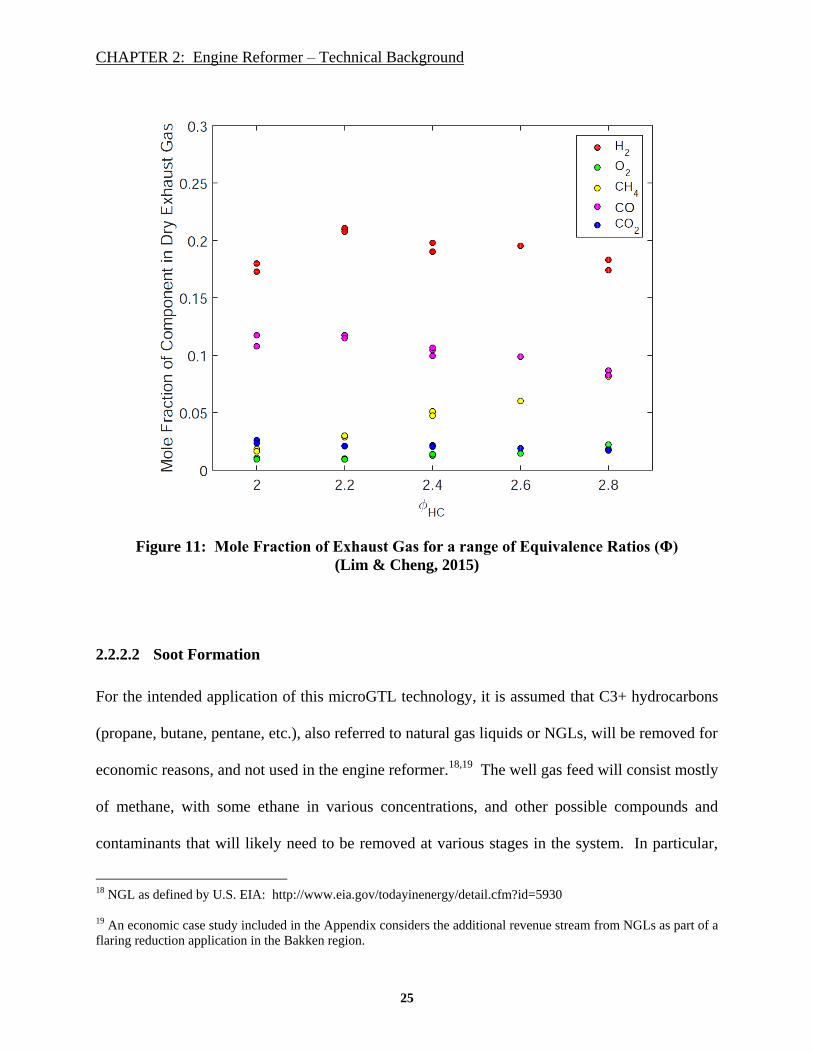
Figure 11 shows the dry mole fractions across a range of Φ for a sample case with inlet pressure
of 1.1 bar absolute and 5% H2 recycle. The general trends for H2:CO ratio and CH4 conversion
vs. Φ can be observed in this chart. Higher Φ results in higher H2:CO ratio along with an
increase in unconverted CH4 in the exhaust.
CHAPTER 2: Engine Reformer – Technical Background
25
Figure 11: Mole Fraction of Exhaust Gas for a range of Equivalence Ratios (Φ)
(Lim & Cheng, 2015)
2.2.2.2 Soot Formation
For the intended application of this microGTL technology, it is assumed that C3+ hydrocarbons
(propane, butane, pentane, etc.), also referred to natural gas liquids or NGLs, will be removed for
economic reasons, and not used in the engine reformer.18,19
The well gas feed will consist mostly
of methane, with some ethane in various concentrations, and other possible compounds and
contaminants that will likely need to be removed at various stages in the system. In particular,
18 NGL as defined by U.S. EIA: http://www.eia.gov/todayinenergy/detail.cfm?id=5930
19 An economic case study included in the Appendix considers the additional revenue stream from NGLs as part of a
flaring reduction application in the Bakken region.

CHAPTER 2: Engine Reformer – Technical Background
26
the likelihood of the presence of ethane in the well gas feed raises the concern for increased soot
formation in the engine.
The formation of soot in the exhaust stream due to the presence of ethane in the inlet feed gas
was tested with the laboratory scale engine at MIT. Figure 12 shows a sampling of results from
the soot formation testing. As might be expected, soot formation is sensitive to Φ, and a sharp
increase in soot formation can be seen at Φ > 2.4. At Φ < 2.2, the soot formation in the exhaust
is between 0.1 and 0.2 mg/L (mg of soot formation per liter of exhaust gas mixture). For a
commercial scale system with 0.33 MMscfd inlet flow of natural gas, 0.1 mg/L of soot will result
in approximately 2.4 kg/day of soot.20
A soot filtration system will be included as part of the
contaminant removal prior to syngas compression in the microGTL system.
It is important to note that the results of the soot formation testing are based solely on the
laboratory scale engine at MIT, and may vary with alternate engine combustion chamber design
and flow characteristics. This laboratory test engine has a flat cylinder head and diesel
combustion chamber modified to accept a spark ignition system. The expected commercial scale
engine will be a dedicated spark-ignition type, and will have non-parallel valves and a domed
piston design. While it is expected that the general trend of increased soot formation with
increased Φ will be present across different types of engine configurations, the extent of the soot
formation vs. engine design is an area of future testing and development.
20 Using an ‘actual volume flow’ from the commercial scale Aspen model (‘manifold exhaust’ stream in Figure 16)
of 1,019 m3/hr: 1,019 m3/hr x 1000 L/m3 x 24 hr/d x 0.1 mg Soot/L x 10^-6 = 2.4 kg/d

CHAPTER 2: Engine Reformer – Technical Background
27
Figure 12: Soot Concentration vs. Equivalency ratio, Φ
(Lim & Cheng, 2015)
2.2.2.3 Sensitivity to Compression Ratio
The Yanmar diesel engine tested at MIT has a compression ratio of 18.9:1. The pilot scale
engine, which has already been selected as of the writing of this thesis is a larger displacement,
dedicated natural gas spark-ignition system with a lower compression ratio. The expectation for
the commercial scale system is that multiples of the pilot scale engine will be used to achieve the
required engine reformer volume. While the compression ratio of a spark-ignition engine can
straightforwardly be increased with a change to piston configuration, the compression ratio will

CHAPTER 2: Engine Reformer – Technical Background
28
not reach that of the laboratory scale engine due to the domed piston and angled intake and
exhaust valves. With this in mind, a reduced compression ratio configuration was tested on the
MIT engine by modifying an existing diesel piston to partially simulate and evaluate the engine
reformer performance. The compression ratio was reduced to 13.8:1 by removing material from
the top of the existing diesel piston. The testing procedure and results are discussed in detail in
Lim & Cheng, 2015, and will not be reviewed in detail here, but the overall findings were that
under similar inlet and operating conditions, the engine reformer system was able to achieve
H2:CO ratios very similar to that of the baseline, higher compression configuration.

CHAPTER 3: Integrated System - Aspen HYSYS Model
29
CHAPTER 3: Integrated System - Aspen HYSYS Model
3.1 System Overview
The techno-economic analysis of the commercial scale engine-reformer based microGTL system
is a significant deliverable as part of this Ph. D. thesis. An Aspen HYSYS (V8.6) model was
constructed to model the commercial scale system and serves as a basis for the economic
analysis. This model was used to estimate the size and cost for several of the system sub-
components, and provide estimates for the heat and power inputs and outputs to estimate the
overall system heat/power budget. Where applicable, the sub-system heat and power flows were
considered as part of integrated loops to meet internal heat and power requirements. Throughout
the system development, the Aspen model is used to inform design and system configuration
decisions for the pilot and commercial scale systems and as a tool to evaluate a range of possible
system operating conditions for particular use cases.
In this section, one possible (likely) commercial scale case, with 60% overall methanol
conversion and a 5% H2 recycle stream, is used as the baseline to review the Aspen model layout
and performance of an anticipated commercial scale, integrated, microGTL system. The values
represented in the stream tables are based on this particular scenario, recognizing that other
outcomes are possible under alternate operating conditions. Figure 13 shows a simple block

CHAPTER 3: Integrated System - Aspen HYSYS Model
30
flow diagram of the commercial scale system while Figure 14 is a high level Aspen process flow
diagram for the same commercial system.
Figure 13: Simple block flow diagram
Figure 14: Aspen HYSYS process flow diagram
CHAPTER 3: Integrated System - Aspen HYSYS Model
31
The individual system components will be reviewed in detail below, but the general flow is as
follows (from left-to-right and top-to-bottom):
The inlet natural gas feed (mostly methane and in some cases mixed with ethane) mixes
with air (MIX-100). The mixed gas is pre-heated using excess heat from the engine
reformer exhaust. The H2 recycle input is included here as well, but it is possible that the
H2 recycle input could enter the system at a point downstream. A preconditioning step
may be included here as well to remove contaminants such as hydrogen sulfide (H2S),
and to remove water and NGLs.
The pre-heated inlet feed (stream #2) is boosted (Super_Charger), and then enters the
four-stroke engine reformer (Stroke1_Intake, Stroke2_Comp, Stroke3_Power,
Stroke3_Combustion, Stroke3_Reaction, Stroke4_Exhaust, Exhaust, Manifold Exhaust).
Manifold exhaust heat is used in a recycle loop to pre-heat the inlet natural gas feed. The
‘Recycle_Exhaust’ loop is made up of residual gases that remain in the combustion
chamber after the exhaust stroke.
The exit feed from the engine after the pre-heat loop is further cooled and liquid water is
dropped out. The remaining dry gas contains H2 and CO at ratios desirable for methanol
synthesis (stream ‘SynGas’). Between the engine reformer and the compressor stages,
syngas conditioning steps (i.e. contaminant removal) will take place that are not
represented in this process flow diagram (this differs slightly from the process order as
displayed in the earlier conceptual layout, Figure 8).
The ‘SynGas’ feed runs through a two-stage compression step (Reactor Comp 1, Reactor
Comp 2) and the pressurized syngas is fed to the methanol reactor system, with liquid

CHAPTER 3: Integrated System - Aspen HYSYS Model
32
methanol as the end product (‘Liquid_Dropout_1’ and ‘Liquid_Dropout_2’). The origin
of a H2 recycle loop will likely be present within or after the methanol reactor system,
with the precise location of the H2 recycle loop subsystem determined after the pilot scale
system is operational.
In the following sections, the individual components in the Aspen model will be reviewed in
more detail.
3.1.1 Inlet Feed Gas, Mixing, Boost, and Pre-heat
Figure 15 is a diagram for the inlet gas feed mixing, air boost, and pre-heating processes,
showing the inlet gas feed of well gas (mainly CH4) and air. Table 1 is a summary of the
relevant stream data. The gas mixture includes additional inputs for a range of C2H6 (ethane)
and H2 recycle concentrations. Ethane concentration from the well gas will vary, with an
anticipated range from 0% to 10%. As mentioned in section 2.2.2.2, a gas mix containing ethane
may contribute to an increase in the formation of soot (and impact Φ), and will need to be
managed through filtering and scheduled maintenance. The H2 recycle stream will come from
the output of the methanol reactor. The H2 recycle loop is represented as an open-loop in Figure
14 and mixes with the inlet gas feed in this case. It is possible in the commercial system
configuration that the recycled H2 could enter the system at a location downstream of the engine
reformer system. A water-gas-shift reactor and H2 membrane system will be incorporated into
the commercial system (and are included in the economic analysis) to provide the pure H2
recycle stream. The H2 recycle is necessary to achieve the desired H2:CO ratio.

CHAPTER 3: Integrated System - Aspen HYSYS Model
33
The inlet air is boosted from atmospheric pressure (1 bar) to 2 bar through an engine driven
supercharger. The supercharger is modeled in Aspen as a reciprocating compressor with
adiabatic efficiency of 0.75. The well gas is assumed to exit the well above atmospheric pressure,
and is conservatively assumed to be 2 bar in this case. The boosted inlet mixture is then
preheated to 350 °C using excess heat from the engine reformer exhaust. The values in Table 1
show the inlet composition for a case with equivalence ratio Φ = 2 (equal mole fractions for CH4
and O2, reviewed in section 2.2.2.1). The natural gas feed composition is 100% CH4 (0%
ethane), and the “Air” stream is comprised of 79% N2 and 21% O2 only (i.e. dry). The flow rate
is equivalent to 0.3 MMscfd of natural gas.21
Figure 15: Inlet feed, mixing, boost, and pre-heat
21 For the CH4 stream, using 22.4 L/mol for the standard molar volume, the commercial scale flow of 0.3 MMscfd is
confirmed by: (16 kgmole/hr) x (22.4 L/mol) x (m3/1000 L) x (35.3 ft3/m3) x (24 hr/d) = 300,000 scfd

CHAPTER 3: Integrated System - Aspen HYSYS Model
34
Table 1: Stream table summary - inlet feed, mixing, boost, and pre-heat
3.1.2 Engine Reformer
3.1.2.1 Overview of Aspen Engine Reformer System
Aspen does not include a component set for an internal combustion engine. With this limitation,
a series of unit operations were constructed in Aspen to simulate the characteristics of the four-
stroke internal combustion engine to extract the information needed for input into the economic
model for the commercial scale microGTL system and to provide estimates for the net power
output from the engine and excess heat available for use in other processes in the overall system.
This zero-dimensional thermodynamic model of the engine reformer is not designed to achieve
1st-principles results, but instead is intended to provide a description of the engine that can be
used to evaluate trends as changes are made to engine parameters within a confined operating
space, providing some predictive capabilities for the overall system model. This engine reformer
CH4 Air Air_Boost C2H6 H2 Recycle To_Preheat Intake_1
Comp Mole Frac Methane 1 0 0 0 0 0.1607 0.1607
Comp Mole Frac Ethane 0 0 0 1 0 0 0
Comp Mole Frac H2O 0 0 0 0 0 0 0
Comp Mole Frac Nitrogen 0 0.79 0.79 0 0 0.6231 0.6231
Comp Mole Frac Oxygen 0 0.21 0.21 0 0 0.1656 0.1656
Comp Mole Frac Hydrogen 0 0 0 0 1 0.0506 0.0506
Comp Mole Frac CO 0 0 0 0 0 0 0
Comp Mole Frac CO2 0 0 0 0 0 0 0
Comp Mole Frac Methanol 0 0 0 0 0 0 0
Vapour Fraction 1 1 1 1 1 1 1
Temperature (deg C) 25.00 25.00 109.31 25.00 25.00 88.91 350.00
Pressure (kPa) 200.00 101.32 200.00 200.00 200.00 200.00 200.00
Molar Flow (kgmole/h) 16.00 78.55 78.55 0 5.04 99.59 99.59
Mass Flow (kg/h) 256.68 2266.20 2266.20 0 10.16 2533.04 2533.04

CHAPTER 3: Integrated System - Aspen HYSYS Model
35
model captures the physics and chemistry of the complete engine model based on known
stoichiometry, and does not consider path and intermediate products.
Figure 16 is a high-level flow diagram for the four-stroke engine reformer system model in
Aspen, and includes a recycle loop for the residual gasses remaining in the cylinder after the
partial combustion reaction. Table 2 is a summary of the stream data for the engine reformer
system starting from the pre-mixed and pre-heated inlet (‘Intake_2’) and ending at the manifold
exhaust. For overall context, the four strokes for a single combustion chamber of the
reciprocating internal combustion engine are:
1. Intake stroke - intake valve(s) open and the piston travels from top to bottom, creating a
slight vacuum and drawing in the inlet gas mixture.22
2. Compression stroke - with intake and exhaust valves closed, the piston travels from the
bottom to top of the cylinder, compressing the gas mixture.
3. Power stroke - with the gas mixture compressed, a spark is introduced to the cylinder,
igniting the gas mixture and initiating the combustion reaction. The energy created
during the reaction pushes the piston down, producing work.
4. Exhaust stroke – exhaust valve(s) open and piston moves from bottom to top, pushing the
exhaust gas mixture out of the cylinder.
22 Engine valvetrain configurations can consist of single or multiple intake and/or exhaust valves. The detail does
not alter the fundamental characteristics of the four-stroke engine cycle.
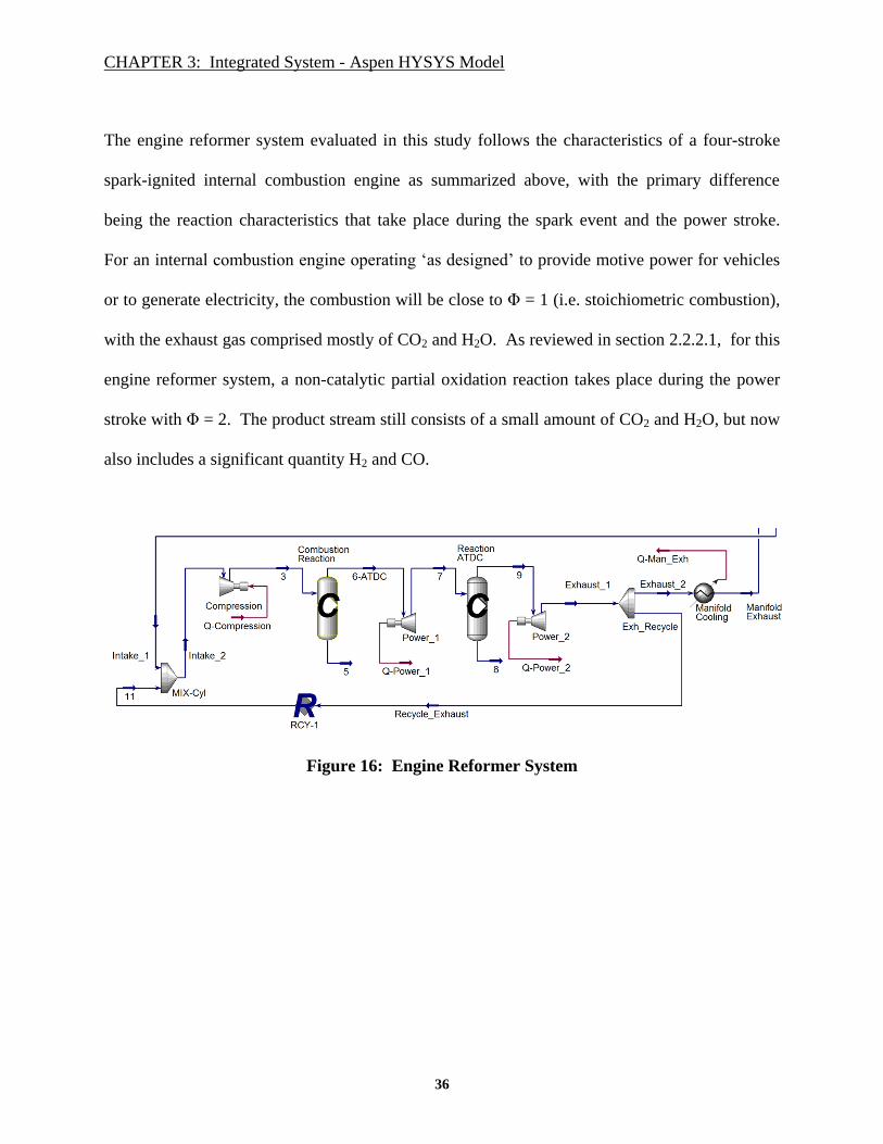
CHAPTER 3: Integrated System - Aspen HYSYS Model
36
The engine reformer system evaluated in this study follows the characteristics of a four-stroke
spark-ignited internal combustion engine as summarized above, with the primary difference
being the reaction characteristics that take place during the spark event and the power stroke.
For an internal combustion engine operating ‘as designed’ to provide motive power for vehicles
or to generate electricity, the combustion will be close to Φ = 1 (i.e. stoichiometric combustion),
with the exhaust gas comprised mostly of CO2 and H2O. As reviewed in section 2.2.2.1, for this
engine reformer system, a non-catalytic partial oxidation reaction takes place during the power
stroke with Φ = 2. The product stream still consists of a small amount of CO2 and H2O, but now
also includes a significant quantity H2 and CO.
Figure 16: Engine Reformer System

CHAPTER 3: Integrated System - Aspen HYSYS Model
37
Table 2: Stream table summary, engine reformer system
3.1.2.2 Aspen Engine Reformer Model Steps
The pre-heated, boosted inlet gas mixture is fed to the engine during the intake stroke
(‘Intake_2’), and compressed during the compression stroke. For the partial oxidation reaction
to occur, the spark timing must be adjusted relative to stoichiometric combustion. Based on
laboratory results at MIT (Lim & Cheng, 2015), the spark timing required for Φ = 2 is
approximately 35 degrees before top dead center (BTDC). Using the slider-crank model for
reciprocating engines, equation (4), with 13.8 compression ratio, 3.5 ratio for connecting rod
length to crank radius, and 4.35 inch / 4.5 inch bore and stroke, the volumetric ratio (V/Vd) at 35
degrees BTDC is 0.19. Based on this volumetric ratio and the defined inlet temperature and
pressure (350 °C, 200 kPa, stream ‘Intake_2’ in Table 2, the cylinder pressure at the start of the
spark event is calculated to be approximately 2,000 kPa (stream #3 in Table 2).
Intake_2 3 6-ATDC 7 9 Exhaust_1/2 Manifold Exh
Comp Mole Frac Methane 0.1607 0.1607 0.0139 0.0139 0.0014 0.0014 0.0014
Comp Mole Frac Ethane 0 0 0 0 0 0 0
Comp Mole Frac H2O 0 0 0.1208 0.1208 0.1311 0.1311 0.1311
Comp Mole Frac Nitrogen 0.6231 0.6231 0.5376 0.5376 0.5303 0.5303 0.5303
Comp Mole Frac Oxygen 0.1656 0.1656 0.0154 0.0154 0.0026 0.0026 0.0026
Comp Mole Frac Hydrogen 0.0506 0.0506 0.1931 0.1931 0.2052 0.2052 0.2052
Comp Mole Frac CO 0 0 0.1028 0.1028 0.1115 0.1115 0.1115
Comp Mole Frac CO2 0 0 0.0165 0.0165 0.0179 0.0179 0.0179
Comp Mole Frac Methanol 0 0 0 0 0 0 0
Vapour Fraction 1 1 1 1 1 1 1
Temperature (deg C) 350.00 905.09 1858.66 1665.11 1761.79 1227.74 250.00
Pressure (kPa) 200.00 2026.50 6635.50 3500.00 3500.00 500.00 500.00
Molar Flow (kgmole/h) 99.59 99.59 115.43 115.43 117.02 117.02 117.02
Mass Flow (kg/h) 2533.04 2533.04 2533.04 2533.04 2533.04 2533.04 2533.04

CHAPTER 3: Integrated System - Aspen HYSYS Model
38
V/Vd = 1/(r-1) + 0.5[1 + R – cosΘ – (R2 – sin
2Θ)
1/2],
where: r = compression ratio,
R = rod length / crank radius,
Θ = crank position (spark timing),
Vd = displacement volume = Π x bore2 x stroke / 4
(4)
The power, ‘Q-Compression’ (Figure 16), required for the compression stroke from the end of
the intake stroke (BDC) to the start of the reaction is estimated in Aspen using a reciprocating
compressor with adiabatic efficiency of 0.75. Based on the engine laboratory results, it is
assumed that the partial oxidation reaction occurs from 35 degrees BTDC to 20 degrees after top
dead center (ATDC). The reaction set, modeled using Aspen Conversion Reactors (C,
‘Combustion Reaction’ and ‘Reaction ATDC,’ Figure 17), will be reviewed in more detail in the
next section, and will be introduced here as it pertains to the overall engine reformer system.
The partial oxidation reaction steps and the engine power output are shown in Figure 17 as part
of the engine power stroke. The reaction begins before TDC and continues through to the start
of the power stroke. This reaction is represented by the first Conversion Reactor in Figure 17.
The pressure at Stream #6-ATDC in Table 2 is calculated by Aspen. This value, 6,636 kPa, is
less than the peak cylinder pressure of 8,500 kPa measured during laboratory testing which
occurred close to TDC. The pressure at Stream #6-ATDC corresponds to the timing of the
reaction at 20 degrees ATDC.

CHAPTER 3: Integrated System - Aspen HYSYS Model
39
Figure 17: Engine reformer – power & reaction stroke
The second conversion reactor shown in Figure 17 is intended to capture the remaining reaction
step that takes place during the power stroke. ‘Q-Power_1’ and ‘Q-Power_2,’ modeled as
expanders with adiabatic efficiency of 0.75, sum to estimate the overall power stroke output.
The pressure for stream #7 (3,500 kPa, Table 2) is calculated as the minimum cylinder pressure
prior to the start of exhaust stroke. This value is calculated based on the pressure, temperature,
and estimated cylinder volume from Stream #6-ATDC to Stream #7. The remaining reaction
takes place under assumed constant volume conditions, with a small increase in both temperature
and molar flow in Stream #9 (Table 2) representing this reaction. The pressure for the
‘Exhaust_1’ stream is defined at 500 kPa based on the intended exit gas pressure from the engine
reformer system. For the actual engine reformer system, the elevated exhaust pressure is
achieved through modified exhaust valve timing and is incorporated to reduce the compression
requirements for the syngas compressor downstream of the engine reformer.

CHAPTER 3: Integrated System - Aspen HYSYS Model
40
The volumetric ratio calculations used to simulate the actual engine operating conditions
(relative to 13.8 overall compression ratio) for the Aspen engine reformer model are summarized
in Table 3, and a table of the detailed stream material properties is included in Appendix B
(Table 41).
Table 3: Volumetric ratio values used for Aspen Engine Reformer model
3.1.2.3 Aspen Engine Reformer Reactions
A set of Aspen conversion reactors were used to model the partial oxidation reaction steps. The
same reaction equation set is used for both Aspen conversion reactors, ‘Combustion Reaction’
and ‘Reaction ATDC’ in Figure 17. The internal combustion chamber reaction equation
necessary to ultimately result in the desired H2:CO ratio at the engine reformer exhaust outlet
was empirically derived based on the exhaust composition taken from the experimental engine
data. The inlet concentration was based on engine dynamometer test data for the specific test
case for an equivalence ratio of Φ = 2, with 5% H2 recycle. The inlet gas mixture concentration
(‘To_Preheat’ stream in Table 1) is expressed as:
0.1607 CH4 + 0.1656 O2 + 0.6231 N2 + 0.0506 H2 (5)
Crank Position V / Vd designation V / Vd Vd / V
35 deg BTDC V_3 / V_Int_2 0.19 5.36
20 deg ATDC V_6 / V_Int_2 0.12 8.37
power stroke end V_9 / V_Int_2 0.22 4.56
exhaust stroke start V_Exh_1 / V_Int_2 1.13 0.88

CHAPTER 3: Integrated System - Aspen HYSYS Model
41
and includes the 5% (by component mole fraction) H2 stream.23
The exhaust recycle is
incorporated into the system downstream of the inlet. Normalized to one mole of methane at the
inlet, Equation (5) takes the form:
CH4 + 1.0305 O2 + 3.8774 N2 + 0.3148 H2 (6)
On a mole fraction basis, the engine reformer exhaust stream concentration (‘Manifold Exh’
stream in Table 2), based on engine dynamometer test data, is expressed as:
0.0014 CH4 + 0.1311 H2O + 0.5303 N2 + 0.0026 O2 + 0.2052 H2 + 0.1116 CO + 0.0179 CO2 (7)
To arrive at the desired exhaust gas concentration in Equation (7), internal reaction sets needs to
be defined for the Aspen conversion reactors. Assuming the N2 in the air inlet stream passes
through the engine reformer system unreacted and the O2 is consumed, the internal Aspen
conversion reactor equation based on the equivalence ratio of Φ = 2 and 5% H2 recycle is
determined empirically from the MIT engine laboratory testing as follows:
CH4 + 1.022 O2 1.198 H2 + 0.824 CO + 0.132 CO2 + 0.968 H2O (8)
Accounting for the 5% H2 recycle, the products from Equation (8) result in a H2:CO ratio of
1.84.24
This overall ratio is obtained by adding the H2 fraction from Equation (6) to the H2
fraction from Equation (8) and dividing by the CO fraction from Equation (8):
(0.3148 H2 + 1.198 H2) / 0.824 CO = 1.84 (9)
23 Note that the actual mole fractions from the experimental data differ very slightly from the ideal case for
equivalence ratio Φ = 2 (1.030 mole O2 actual vs. 1.000 mole O2 by definition for Φ = 2).
24 H2: 1.198 + 0.3148 = 1.5128; 1.5128 H2 / 0.824 CO = 1.84

CHAPTER 3: Integrated System - Aspen HYSYS Model
42
Figure 18 shows the reaction equation inputs to the Aspen model used for both conversion
reactors. A 90% methane conversion is used for the reaction, and results in a 99% overall
methane conversion after the gas mixture passes through the second reactor.
Figure 18: Reaction coefficients for engine reformer combustion/reaction stroke
On a dry basis (after the water is dropped out), the carbon balance for the system described by
the Aspen model is estimated at approximately 93%, with the remaining carbon contributing to
soot formation (experimental results pertaining to soot formation are reviewed in section
2.2.2.2). The ‘SynGas’ stream flow in Table 5 is the basis for calculating the carbon balance as
follows:
100 x (0.0014 CH4 + 0.1273 CO + 0.0204 CO2) / 0.1607 CH4 = 92.78 % (10)

CHAPTER 3: Integrated System - Aspen HYSYS Model
43
The numerator values in equation (10) are the carbon products in the ‘SynGas’ stream flow, and
the denominator is the methane mole fraction in the inlet gas mixture. The exact quantity of
soot formation cannot straightforwardly be determined from this Aspen model configuration
because the reaction sets have been defined based on a predetermined output. It is possible
however to perform a parallel study in Aspen to evaluate the sensitivity of soot formation. The
current Aspen model carbon balance is conservative in terms of soot formation, as the
experimental results (section 2.2.2.2) show a lower quantity of soot in the exhaust gas. With
existing information from experimental results, and the lack of detailed clean-up steps in the
Aspen model, exploring soot formation in more detail in the Aspen model is outside the scope of
the use for the current model.
3.1.2.4 Aspen Engine Reformer Exhaust Heat Utilization and Liquid Drop-out
A close-up of the exhaust system is shown in Figure 19 and includes the exhaust stroke from the
engine, the exhaust manifold, and the heat exchanger loop for the inlet gas mixture pre-heat step.
An external cooler (‘Cooler into Syngas Separator_2’) is also included to account for any
additional cooling requirements necessary to reduce the exhaust stream temperature to drop out
liquid water. The stream values for these steps are summarized in Table 4.
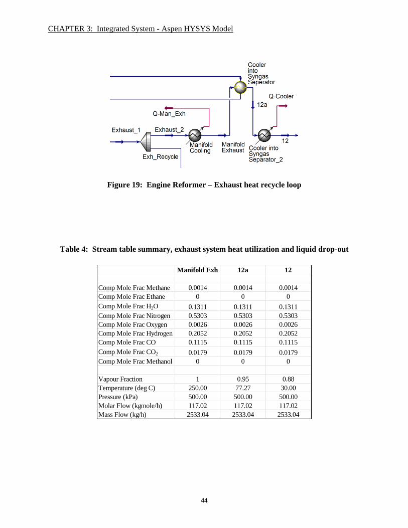
CHAPTER 3: Integrated System - Aspen HYSYS Model
44
Figure 19: Engine Reformer – Exhaust heat recycle loop
Table 4: Stream table summary, exhaust system heat utilization and liquid drop-out
Manifold Exh 12a 12
Comp Mole Frac Methane 0.0014 0.0014 0.0014
Comp Mole Frac Ethane 0 0 0
Comp Mole Frac H2O 0.1311 0.1311 0.1311
Comp Mole Frac Nitrogen 0.5303 0.5303 0.5303
Comp Mole Frac Oxygen 0.0026 0.0026 0.0026
Comp Mole Frac Hydrogen 0.2052 0.2052 0.2052
Comp Mole Frac CO 0.1115 0.1115 0.1115
Comp Mole Frac CO2 0.0179 0.0179 0.0179
Comp Mole Frac Methanol 0 0 0
Vapour Fraction 1 0.95 0.88
Temperature (deg C) 250.00 77.27 30.00
Pressure (kPa) 500.00 500.00 500.00
Molar Flow (kgmole/h) 117.02 117.02 117.02
Mass Flow (kg/h) 2533.04 2533.04 2533.04

CHAPTER 3: Integrated System - Aspen HYSYS Model
45
‘Q-Man_Exh’ represents an estimate of the available heat from the engine exhaust stream.
While a portion of this heat is currently used as pre-heat step for the inlet mixture, there is a large
quantity of available heat that is not yet utilized but is available if needed. The Aspen model
results estimate the exhaust gas temperature at the cylinder head exit to be approximately 1,230
°C (‘Exhaust_1/2,’ Table 2). While the Aspen model was free to calculate the internal engine
temperatures based on the inlet conditions and reactions, the exhaust manifold exit temperature
(250 °C) was fixed so that a consistent baseline temperature could be used for downstream heat
management and stream flow characteristics. The actual configuration of the commercial scale
engine reformer exhaust system may result in a slightly different exit temperature for the
manifold component.
In addition to utilizing excess heat and power from the engine reformer system, another
important characteristic of this system is the increased exhaust gas pressure that is anticipated
based on design modifications to the exhaust valve timing. An expected engine exhaust pressure
of 5 bar (500 kPa) is fixed in the ‘Exhaust’ stream. The inlet gas mixture pressure boost from the
inlet supercharger combined with the exhaust valve timing modification contribute to this
pressure increase. The potential for a further increase in exhaust gas pressure from the engine
reformer system will be studied for the commercial scale system. Higher exhaust pressures will
likely result in the need to redesign the exhaust manifold system, adding to component capital
costs. This Aspen model will be used to inform the comparison between additional component
cost from the exhaust manifold redesign versus the reduction in external compressor size and
cost requirements to arrive at an optimum. In the economic analysis in the following chapter, it
will be shown that the 2-stage syngas compression contributes approximately 50% to the overall

CHAPTER 3: Integrated System - Aspen HYSYS Model
46
system capital cost. With this in mind, any additional compression that the engine may provide
should come at a cost that is considerably less than that of the compressor system itself.
3.1.3 Syngas Compression
The H2 and CO rich exhaust gas exits the engine reformer system (stream #12, Table 4) and
passes through a water separator step (Figure 20). In the case used for this system review, the
inlet air mixture is dry, so only produced water from the engine reformer reaction steps are
present in the exhaust gas feed. This water is removed and a dry gas feed enters the syngas
compressor. The stream flow data in Table 5 shows the composition (mole fraction) of the
‘SynGas’ feed. After the water dropout, more than half of the ‘SynGas’ stream composition is
unreacted N2 (60%), followed by H2 and CO at a H2:CO ratio of 1.84 (36%), and the remaining
4% made up of CO2, and very small amounts of O2 unreacted CH4.
The inlet gas mixture used in this high-level model does not consider the range of possible
contaminants that may be present in the natural gas feed. Contaminant removal steps will take
place after the engine reformer and prior to the syngas compression. The contaminant removal
steps are considered in the economic model for the commercial system in Chapter 4. The
contaminant removal requirements will be dictated by the methanol reactor design requirements
for the syngas feed. The economic analysis in Chapter 4 includes a sensitivity study around a
range of capital cost values that inherently includes a range of component costs for the
contaminant removal.

CHAPTER 3: Integrated System - Aspen HYSYS Model
47
Figure 20: ‘SynGas’ feed and water separation
After contaminant removal, the dry ‘SynGas’ stream feeds into the compression step. The
‘SynGas’ stream enters the compressor at 5 bar from the engine reformer, and is compressed to
45 bar through a 2 stage compressor system (Figure 21). The 45 bar inlet pressure requirement
in the current methanol reactor design specification accounts for the N2 content in the stream.
The calculated compressor power requirements from the Aspen model, ‘Q-reactor_Comp_1’ and
‘Q-reactor_Comp_2,’ provide estimates for the overall system power and heat budget, and will
be reviewed in the following section. An intercooler step is included in the model and is
adjustable based on the inlet and exit pressure values and exit temperature requirement.
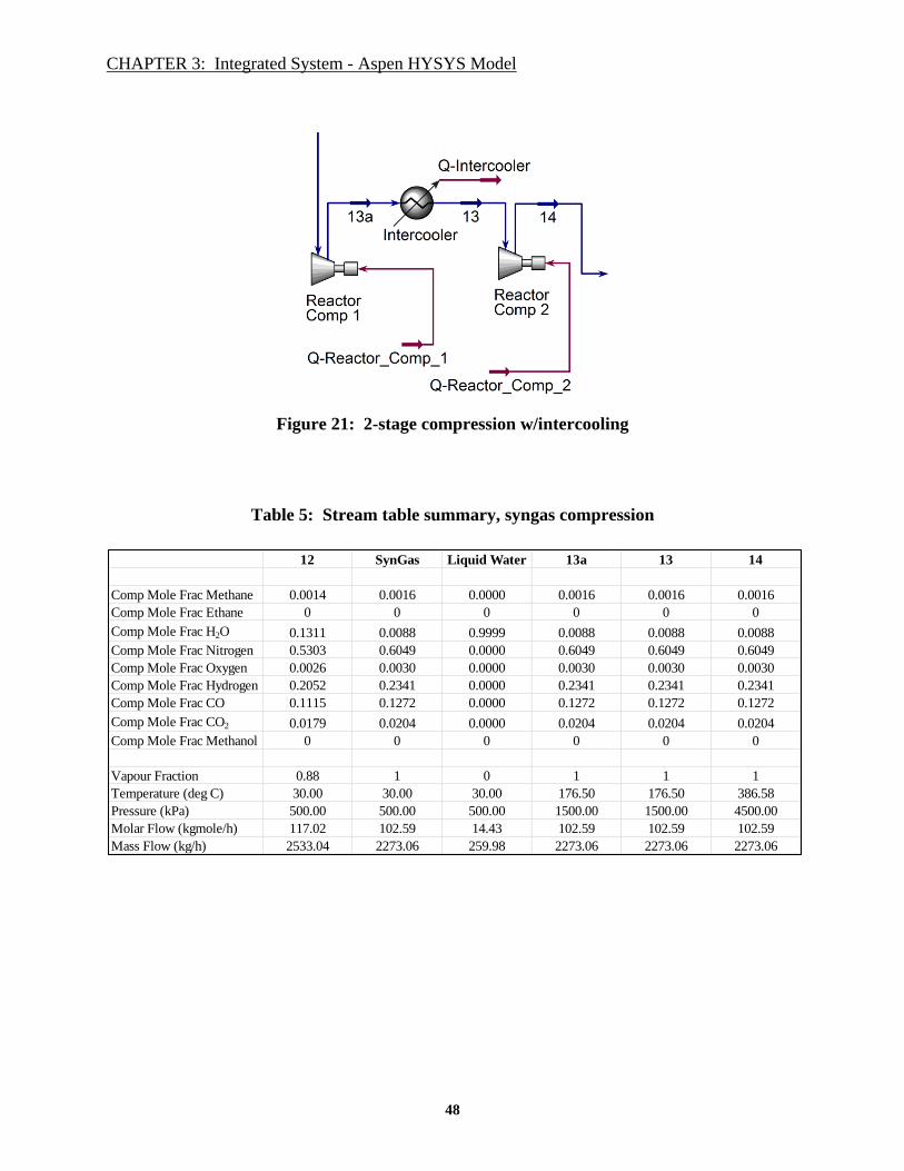
CHAPTER 3: Integrated System - Aspen HYSYS Model
48
Figure 21: 2-stage compression w/intercooling
Table 5: Stream table summary, syngas compression
12 SynGas Liquid Water 13a 13 14
Comp Mole Frac Methane 0.0014 0.0016 0.0000 0.0016 0.0016 0.0016
Comp Mole Frac Ethane 0 0 0 0 0 0
Comp Mole Frac H2O 0.1311 0.0088 0.9999 0.0088 0.0088 0.0088
Comp Mole Frac Nitrogen 0.5303 0.6049 0.0000 0.6049 0.6049 0.6049
Comp Mole Frac Oxygen 0.0026 0.0030 0.0000 0.0030 0.0030 0.0030
Comp Mole Frac Hydrogen 0.2052 0.2341 0.0000 0.2341 0.2341 0.2341
Comp Mole Frac CO 0.1115 0.1272 0.0000 0.1272 0.1272 0.1272
Comp Mole Frac CO2 0.0179 0.0204 0.0000 0.0204 0.0204 0.0204
Comp Mole Frac Methanol 0 0 0 0 0 0
Vapour Fraction 0.88 1 0 1 1 1
Temperature (deg C) 30.00 30.00 30.00 176.50 176.50 386.58
Pressure (kPa) 500.00 500.00 500.00 1500.00 1500.00 4500.00
Molar Flow (kgmole/h) 117.02 102.59 14.43 102.59 102.59 102.59
Mass Flow (kg/h) 2533.04 2273.06 259.98 2273.06 2273.06 2273.06

CHAPTER 3: Integrated System - Aspen HYSYS Model
49
3.1.4 Methanol Reactor
The design and development of the methanol reactor system is underway as of the writing of this
thesis through a joint development effort between Casale SA and RTI. Casale, a Swiss company,
is a global leader in methanol synthesis technology. Casale recognizes the need for small-scale,
distributed methanol production and has agreed to design and build the prototype methanol
reactor units. The detailed, internal performance characteristics of the Casale methanol reactor
system are considered a “black box” throughout this system analysis. The inlet feed
requirements were defined along with an overall conversion percentage to arrive at a production
rate of approximately 6 ton per day of liquid methanol. Based on the specific syngas
composition delivered from the engine reformer system, the required inlet temperature and
pressure to the methanol reactor system are 250 °C and 45 bar per direction from Casale. The
inlet requirements for the methanol reactor account for the presence of N2 in the syngas stream.
The methanol production rate is based on an inlet feed of 0.33 MMscfd of natural gas and an
overall methanol reactor system conversion of 60%.
The Aspen model is simplified to include two conversion reactors with a defined reaction set and
a per-reactor methanol conversion percentage to arrive at a 60% overall system conversion. The
system economic analysis in the next chapter includes a sensitivity study around the methanol
reactor system conversion percentage. Figure 22 shows the general layout of the methanol
reactor system in the Aspen model used for the economic analysis. Table 6 andTable 7 provide a
summary of the methanol reactor system stream characteristics. A small pressure drop internally
across the reactors is likely in the physical system (approximately 5 psi, or 35 kPa). Due to the
magnitude of the pressure drop (< 1% of the overall stream pressure), a zero pressure drop is

CHAPTER 3: Integrated System - Aspen HYSYS Model
50
assumed internally across the reactors for this analysis. The internal pressure values through the
methanol reactor system are summarized in the stream flow data in Table 6 andTable 7.
Figure 22: Methanol reactor (black box)
As mentioned above, the current methanol reactor system requires an inlet feed at 45 bar, which
accounts for the N2 in the syngas gas stream. A series of internal heat exchangers are included in
the methanol reactor system to achieve the required reactor inlet temperature of 250 °C using
excess heat from within the system. The reactor outlet stream is then cooled to dropout the
liquid methanol and water in both of the reactors (‘Methanol Reactor_1’ and ‘Methanol
Reactor_2’). The simple reaction used for the two conversion reactors in the system (Figure 23)
is:
CO + 2 H2 CH3OH (11)
A 40% conversion for each reactor was determined empirically to result in the overall system
conversion of 60%. Using the stream values from Table 6 andTable 7, the overall methanol
production for this particular scenario is:
(0.818 mole fraction methanol x 5.78 kgmole/h molar flow + 0.970 mole fraction
methanol x 3.18 kgmole/h molar flow) x 32.04 kg/kgmole methanol molar mass x 24
hr/d x ton/1000kg = 6 ton/day methanol
(12)

CHAPTER 3: Integrated System - Aspen HYSYS Model
51
Table 6: Stream table summary, methanol reactor – part 1
Table 7: Stream table summary, methanol reactor – part 2
15 16 18 19 20 Liquid Dropout_1
Comp Mole Frac Methane 0.0016 0.0017 0.0017 0.0017 0.0018 0
Comp Mole Frac Ethane 0 0 0 0 0 0
Comp Mole Frac H2O 0.0088 0.0098 0.0098 0.0098 0.0002 0.1564
Comp Mole Frac Nitrogen 0.6049 0.6734 0.6734 0.6734 0.7172 0.0105
Comp Mole Frac Oxygen 0.0030 0.0033 0.0033 0.0033 0.0036 0.0001
Comp Mole Frac Hydrogen 0.2341 0.1473 0.1473 0.1473 0.1570 0.0006
Comp Mole Frac CO 0.1272 0.0850 0.0850 0.0850 0.0906 0.0005
Comp Mole Frac CO2 0.0204 0.0227 0.0227 0.0227 0.0238 0.0054
Comp Mole Frac Methanol 0.0000 0.0567 0.0567 0.0567 0.0058 0.8266
Vapour Fraction 1 1 1 0.94 1 0
Temperature (deg C) 250.00 418.29 554.38 30.00 30.00 30.00
Pressure (kPa) 4465.53 4465.53 4431.06 4527.58 4527.58 4527.58
Molar Flow (kgmole/h) 102.59 92.14 92.14 92.14 86.44 5.71
Mass Flow (kg/h) 2273.06 2273.06 2273.06 2273.06 2102.68 170.38
21 22 24 25 Vent Liquid Dropout_2
Comp Mole Frac Methane 0.0018 0.0020 0.0020 0.0021 0.0021 0.0001
Comp Mole Frac Ethane 0 0 0 0 0 0
Comp Mole Frac H2O 0.0002 0.0002 0.0002 0.0000 0.0000 0.0042
Comp Mole Frac Nitrogen 0.7172 0.7732 0.7732 0.8045 0.8045 0.0167
Comp Mole Frac Oxygen 0.0036 0.0038 0.0038 0.0040 0.0040 0.0001
Comp Mole Frac Hydrogen 0.1570 0.0912 0.0912 0.0949 0.0949 0.0005
Comp Mole Frac CO 0.0906 0.0586 0.0586 0.0610 0.0610 0.0005
Comp Mole Frac CO2 0.0238 0.0257 0.0257 0.0264 0.0264 0.0079
Comp Mole Frac Methanol 0.0058 0.0453 0.0453 0.0072 0.0072 0.9700
Vapour Fraction 1 1 0.96 1 1 0
Temperature (deg C) 250.00 367.86 30.00 30.00 441.68 30.00
Pressure (kPa) 4500.00 4500.00 4465.53 4465.53 4431.06 4465.53
Molar Flow (kgmole/h) 86.44 80.17 80.17 77.00 77.00 3.18
Mass Flow (kg/h) 2102.68 2102.68 2102.68 2001.04 2001.04 101.63

CHAPTER 3: Integrated System - Aspen HYSYS Model
52
Figure 23: Methanol reactor example reaction coefficients
3.1.4.1 Methanol Reactor – Thermodynamic Equilibrium Analysis
While the inlet and outlet conditions were defined for the methanol reactor system from Casale
(i.e. ‘black box’), it is still worthwhile to confirm that the ‘black box’ conditions are reasonable
estimates compared to thermodynamic equilibrium under similar conditions. Using Aspen Plus
V8.6, a simple methanol reactor system was defined using a Gibbs (‘RGIBBS’) Figure 24. The
RGIBBS reactor determines the equilibrium product composition by minimizing the Gibbs free
energy in the system.

CHAPTER 3: Integrated System - Aspen HYSYS Model
53
Figure 24: Simple Gibbs Reactor in Aspen Plus V8.6
The baseline ‘black box’ conditions discussed earlier in this section were used to compare the
methanol reactor output at thermodynamic equilibrium to the output from the methanol reactor
system in Figure 22. The methanol output from the reactors in Figure 22 is based on the
methanol in stream #16 (and stream #22). The output from these streams is approximately 0.05
methanol by mole fraction. Figure 25 is a plot of the equilibrium results in terms of mole
fraction vs. temperature for the baseline inputs (pressure, inlet gas mixture including N2, flow
rate). The mole fraction for N2 is high compared to the other compounds in Figure 25 (0.60 –
0.68 range), and is not plotted. Under these conditions, similar methanol output is observed
around 220 °C. While not exactly at the 250 °C inlet condition defined by Casale for the
methanol reactor system, this value is close (and achievable). Perhaps more importantly, Figure
25 highlights the sensitivity to temperature for methanol production under the current inlet
conditions, as well as the remaining H2 and CO vs. temperature. If lower temperatures cannot be
achieved, then an additional pass through a reactor may be required to meet the desired system
methanol output.

CHAPTER 3: Integrated System - Aspen HYSYS Model
54
Figure 26 is a plot of the equilibrium results vs. pressure. The baseline temperature was reduced
slightly from 250 °C to more closely match the system methanol output. Similar to the
temperature sensitivity results, the methanol mole fraction at equilibrium is close to the output
from the reactor system in the Aspen model, further confirming that the initial estimates from
Casale are close to the thermodynamic equilibrium. The results plotted in Figure 27 provide an
overall summary of the temperature and pressure sensitivity results for the baseline case used for
the Aspen model. The plot shows that the reactions are sensitive to the partial pressure of the
reactants and reaction products and the impact of the nitrogen present is small.
Figure 25: Temperature vs. Mole Fraction, baseline case

CHAPTER 3: Integrated System - Aspen HYSYS Model
55
Figure 26: Pressure vs. Mole Fraction, baseline case
Figure 27: Temperature & Pressure vs. Methanol Production, baseline case

CHAPTER 3: Integrated System - Aspen HYSYS Model
56
In the interest of understanding the impact that excess N2 has on the overall system scale, a
simple, theoretical case using 95% O2 was evaluated. With the overall conversion efficiency
fixed to the baseline (w/N2) case, adjustments were made to the overall gas mixture mass flow
while maintaining the same CH4 mass flow as in the baseline example (i.e. the carbon flow does
not change in this 95% O2 case).25
The partial pressures for CH4, H2, and CO remain the same
between the baseline and 95% O2 cases as well (the partial pressure of H2 + CO is approximately
16 bar). Figure 28 and Figure 29 show the results for the thermodynamic equilibrium study for
the 95% O2 case for temperature vs. mole fraction and pressure vs. mole fraction, respectively.
Accounting for the reduced mass flow in the 95% O2 case, the methanol production based on the
mole fraction for methanol at 16 bar in Figure 29 is equal to the methanol production for the
baseline case (as expected).
The reason for performing this basic analysis is to provide some initial insight into the impact
that an enriched O2 case can have on the overall microGTL system. The reduced mass flow
combined with the reduced pressure requirement may result in a significantly smaller compressor
system with a lower power requirement. Alternatively, the compressor system could maintain 45
bar outlet compression and take advantage of increased methanol production (approximately
3.5x production based on the results in Figure 29). Additional methanol production may also be
possible by additional recycle loops internal to the methanol reactor system before reaching the
N2 limit in the current Casale system.
25 The molar flow was adjusted from 102.65 kgmole/hr in the baseline case to 40.81 kgmole/hr in the 95% O2 case,
matching the carbon flow and methanol production between cases.
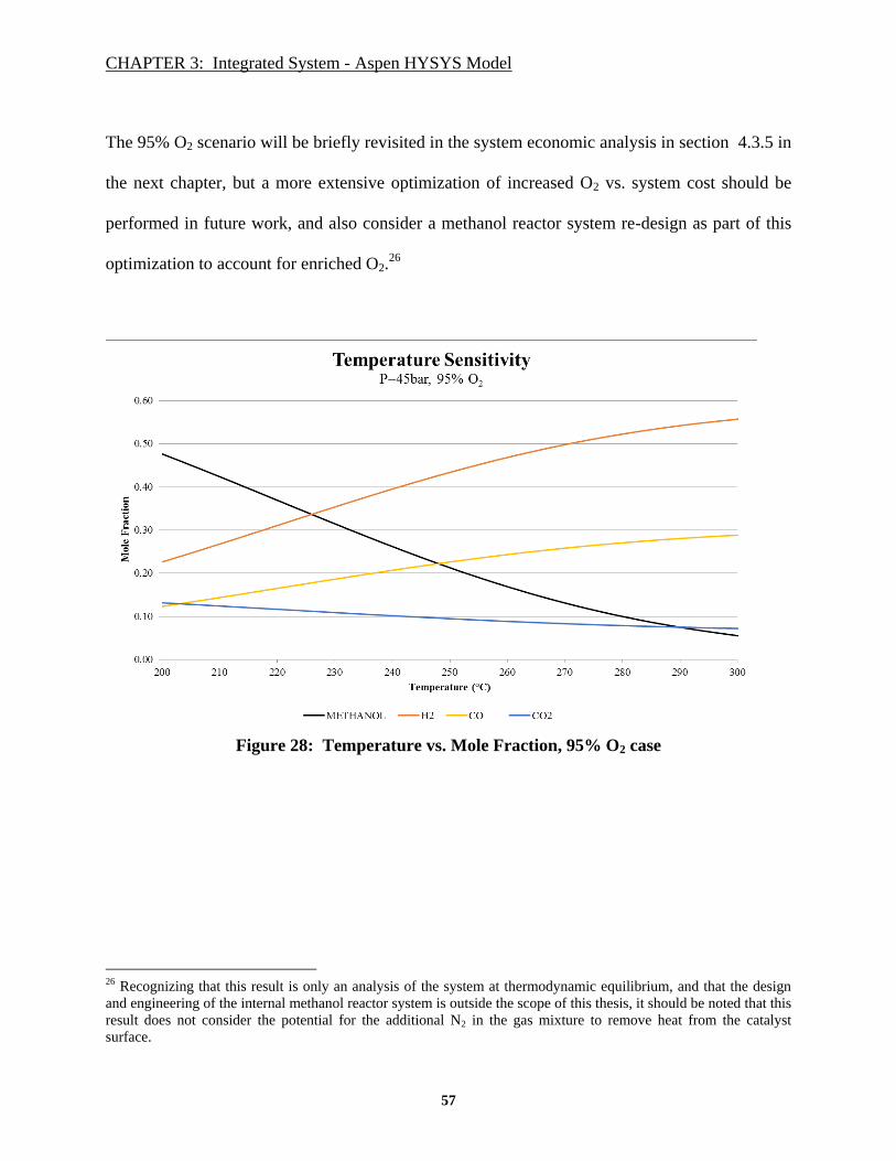
CHAPTER 3: Integrated System - Aspen HYSYS Model
57
The 95% O2 scenario will be briefly revisited in the system economic analysis in section 4.3.5 in
the next chapter, but a more extensive optimization of increased O2 vs. system cost should be
performed in future work, and also consider a methanol reactor system re-design as part of this
optimization to account for enriched O2.26
Figure 28: Temperature vs. Mole Fraction, 95% O2 case
26 Recognizing that this result is only an analysis of the system at thermodynamic equilibrium, and that the design
and engineering of the internal methanol reactor system is outside the scope of this thesis, it should be noted that this
result does not consider the potential for the additional N2 in the gas mixture to remove heat from the catalyst
surface.

CHAPTER 3: Integrated System - Aspen HYSYS Model
58
Figure 29: Pressure vs. Mole Fraction, 95% O2 case
3.1.5 System Energy Budget
The estimates for the power and heat inputs and outputs for the commercial scale integrated
system are presented in Table 8. These results were generated using the Aspen model reviewed
in this chapter for the example case of Φ = 2 with 5% H2 recycle. It is likely that the engine
reformer system will be able to ‘self-power’ based on the excess power and heat generated
through the partial oxidation reaction. Further, it is likely that excess engine power will be used
to direct drive other components from the engine or converted to electricity through a generator
system. The excess heat from the engine reformer exhaust manifold can be utilized for internal
heat-exchanger cycles within the integrated system.

CHAPTER 3: Integrated System - Aspen HYSYS Model
59
Table 8: Component power & heat inputs and outputs from integrated system Aspen
model
Component kW Description
Supercharger, Q-SC -54.1 Engine driven supercharger - Boosts inlet air from 1 to 2 bar
Engine Reformer
Q-Compression 584.8 Compression stroke power requirement
Q-Power_1 257.1 Power stroke output
Q-Power_2 653.7 Continuation of power stroke output
Engine Net Power Out 326.0 Power - Compression
Manifold Exhaust Heat, Q-Man_Exh 1073.7Excess exhaust manifold heat, some of which is utilized for
the inlet gas pre-heat
Q-Cooler -157.3Additional cooling requirement to dropout liquid water after
heat removed for inlet gas pre-heat step
Syngas Compressor
Q-Reactor_Comp_1 -123.5 Stage 1 power requirement
Q-Reactor_Comp_2 -183.9 Stage 2 power requirement
Syngas Power Req -307.4Total compressor power requirement to boost syngas feed
from 5 to 45 bar for Methanol Reactor
Methanol Reactor
Cooler into Reactor_1 -120.9Cooling required to meet 250 °C reactor inlet temperature
requirement
Cooler into Reactor_2 -345.5Cooling required to meet 30 °C liquid dropout followed by re-
heat to 250 °C reactor inlet temperature requirement
Cooler into Separator_2 -277.7 Cooling required to meet 2nd liquid dropout step
Methanol Reactor Cooler Req -744.1

CHAPTER 3: Integrated System - Aspen HYSYS Model
60
The net power output for the engine reformer system is determined by the difference between the
compression and power strokes. The Aspen model calculates the adiabatic compressor (and
expander) power input (and output) using discrete values for the specific heat at constant
pressure (cp) and specific heat at constant volume (cv) for the specific gas composition. The
general form of this adiabatic compression work equation is:
w = γ / (γ -1) R T1 [( P2 / P1)((γ-1)/γ)
- 1]
where γ = cp / cv
(13)
Values for adiabatic efficiency, molar flow, and mass flow are then included to arrive at a power
value for each compressor (or expander) component. Referring to Table 8, the net power output
for the engine reformer system is 326 kW, based on the difference between the power required
for the compression stroke and the power output from the power stroke.27
The engine reformer system also produces a large quantity of excess heat (~1,070 kW) through
the exhaust manifold, represented in Table 8 by ‘Q-Man_Exh.’ This excess heat will be used to
pre-heat the inlet gas mixture, and may also be used to provide heat for heat exchangers to re-
heat the stream after cooling for liquid dropout throughout the system processes. The details of
how to utilize the exhaust heat will be determined during the design of the commercial scale
system; this analysis provides an initial estimate of the magnitude of available heat.
The ‘Q-Cooler’ value in Table 8 is an estimate of the power required for the chiller to cool the
remainder of the exhaust gas mixture (after the pre-heat step) to dropout any produced water
27
Any mechanical losses due to friction in the actual engine are assumed to be accounted for by the adiabatic
efficiency for the individual compressor and expanders in the Aspen model.

CHAPTER 3: Integrated System - Aspen HYSYS Model
61
prior to compression of the dry, syngas-rich gas stream. The syngas compressor power
requirement to compress this gas mixture from 5 bar to 45 bar for the methanol reactor is
estimated at 307 kW through a 2-stage compressor system.
A series of cooling steps are required throughout the methanol reactor system. The first cooling
step reduces the temperature of the gas mixture from the syngas compressor to 250 °C necessary
to enter the methanol reactor. The remaining cooling steps are needed to dropout the liquid
methanol product and any water produced during the reactions. The estimated power values for
these chiller systems are summarized in Table 8, and sum to a net power requirement of ~740
kW.
A likely commercial configuration of the engine reformer system will include a generator to
produce electricity as part of a ‘generator set’ (‘genset’) system. For the case presented here, the
excess power from the engine reformer system should contribute to meeting most/all of the
power requirements for both the supercharger and syngas compression. The remaining system
power requirements are for the chiller systems necessary to cool the gas stream at various steps
throughout the system for liquid dropout of both produced water and methanol. A scenario that
will be explored further in future work for the commercial scale system design will review the
economic case for using on-board engines, running at stoichiometric combustion on natural gas
from the wellhead for the purpose of providing all of the power requirements to run the
microGTL system without the need for external power. The current economic model assumes
that the excess power requirements for the chiller systems are included in the operation and
maintenance cost.

CHAPTER 4: Integrated System - Economic Analysis
62
CHAPTER 4: Integrated System - Economic Analysis
4.1 Estimating Engine Cost
From a technical perspective, the engine reformer system is the novel component in this
microGTL system. Not only can the engine system be used to produce an exhaust stream rich in
H2 and CO, but this system can take advantage of the fact that engines are inexpensive, mass-
produced units. While the fact that engines are cheap is generally well accepted, the question of
‘how cheap?’ needs to be answered. Deriving the component cost of an engine is not entirely
straightforward however, complicated by the fact that most engines are sold either as a
component of a larger system (i.e. a vehicle or generator set) or at a retail. Without transparently
available engine manufacturer cost data, an alternate method needs to be used to arrive at an
engine cost estimate.
The methodology used to derive the engine cost estimate used for the system economic analysis
in this thesis is based on an Argonne National Laboratory (ANL) study that thoroughly evaluates
the vehicle cost structure for passenger vehicles in the United States (Cuenca, Gaines, & Vyas,
1999). This study, published in 1999, has been widely cited in support of other work requiring
detailed vehicle cost estimates.28
A follow-up study, also by ANL and including some of the
same authors, compared the results from their method for estimating vehicle manufacturing costs
28 https://scholar.google.com/scholar?cites=4017666560542468678&as_sdt=5,33&sciodt=0,33&hl=en

CHAPTER 4: Integrated System - Economic Analysis
63
to two other industry studies (Vyas, Santini, & Cuenca, 2000). One of the comparison studies
was derived from published work from Chrysler Corporation (referred to as the Borroni-Bird
method in the Vyas, et al. report), and the other from the Office of Technology Assessment
(OTA) through the United States Congress (referred to as the Energy and Environmental
Analysis, or EEA method). While different methods were used in each of these three studies
(ANL, Borroni-Bird, EEA) to arrive at vehicle component manufacturing estimates relative to
the vehicle’s Manufacturer Suggested Retail Price (MSRP), the overall results between the three
studies were in-line with each other, with the ANL method providing the most granularity.
Based on the results of this comparison study, the ANL report (Cuenca et al., 1999) was
considered as a reasonable source to estimate the engine system manufacturing cost.
Tables 9 and 10 are from the ANL report. From the data in these two tables, the basis for the
engine system cost estimate is derived. These results show that on average, 50% of a vehicle’s
MSRP is attributed to the manufacturing of the vehicle (Table 9), and within the manufacturing
cost component, 18.5% can be attributed to the engine subsystem (Table 10) (Cuenca et al.,
1999). Using these estimates for the share of MSRP attributable to the vehicle manufacturing
combined with the share of manufacturing attributable to the engine unit, an estimate for the
engine manufacturing cost can be derived using a vehicle’s published MSRP. Using this
methodology to arrive at the engine manufacturing cost, a search of publicly-available sources
was used to gather MSRP data for a range of commercially available production vehicles or
direct-sale engines over a range of engine displacements.

CHAPTER 4: Integrated System - Economic Analysis
64
Table 9: Vehicle Manufacturing and Retailing Cost Structure
Table Source: (Cuenca et al., 1999)
Table 10: Vehicle Production Cost Allocation
Table Source: (Cuenca et al., 1999)

CHAPTER 4: Integrated System - Economic Analysis
65
For each vehicle MSRP data point, the ‘base model’ configuration of a particular vehicle model
was selected.29
In the cases for direct-sale commercially available engines (mostly high power
output 8-cylinder “crate engines” from General Motors and Ford), only the 50% manufacturing
factor was applied to the cost calculation. The data in Table 11 provides a summary of the
engines used to arrive at the engine manufacturing cost estimate. The power values are included
for comparison, but are not used for this particular analysis. The “Cylinder Head” and “Block”
columns designate the material of these subcomponents (1: Aluminum, 2: Cast Iron, 3: Steel),
and will be discussed below.
The engine manufacturing cost factors from the ANL report, along with the published MSRP (in
2015 $) for the vehicle are used to arrive at an overall engine cost. For example, using the first
row of data from Table 11:
$13,965 (vehicle MSRP) x 50% manufacturing share of MSRP x 18.5% engine unit
share of manufacturing = $1,292 engine production cost.
(14)
Using the engine displacement for the given vehicle, the engine manufacturing cost in $/liter can
then be determined. From this analysis, the average cost per displacement for the entire data set
is $636/Liter. The average cost per displacement for engines larger than 4 liters of total
displacement is $544/Liter. Figure 30 is a plot of the engine cost on a per liter basis vs. engine
displacement.
29
In other words, if the same engine was available for several different vehicle models, the least expensive
configuration was selected.

CHAPTER 4: Integrated System - Economic Analysis
66
Table 11: Compiled engine cost data
MSRP Engine Disp Power peak Power peak Cylinder Block Engine Cost $/L $/kW HP/Liter engine notes
$ Liter HP kW Head $
$13,965 1.6 120 89.5 1 1 $1,292 $807 $14.44 75.0 1.6L 16-valve Ti-VCT I-4
$16,950 1.8 132 98.4 1 1 $1,568 $871 $15.93 73.3 Toyota ZZ engine
$17,250 1.8 148 110.4 1 1 $1,596 $886 $14.46 82.2 Nu Mpi 1.8L
$17,995 1.8 170 126.8 1 2 $1,665 $925 $13.13 94.4 Turbo
$16,170 1.8 138 102.9 1 2 $1,496 $831 $14.53 76.7 GM Family II engine
$18,290 1.8 143 106.6 1 1 $1,692 $940 $15.87 79.4 R18A1
$17,170 2.0 160 119.3 1 1 $1,588 $794 $13.31 80.0
$21,600 2.0 174 129.8 1 1 $1,998 $999 $15.40 87.0 Nu GDi 2.0L
$22,345 2.0 150 111.9 1 2 $2,067 $1,033 $18.48 75.0 TD
$21,650 2.0 164 122.3 3 2 $2,003 $1,001 $16.38 82.0 Theta Series
$22,105 2.4 185 138.0 1 1 $2,045 $852 $14.82 77.1 K series
$23,700 2.4 182 135.7 3 2 $2,192 $913 $16.15 75.8 Theta II
$22,970 2.5 178 132.7 1 1 $2,125 $850 $16.01 71.2 2AR-FE
$21,120 2.5 $1,954 $781 Chevy Colorado
$25,800 3.5 282 210.3 1 1 $2,387 $682 $11.35 80.6
$30,495 3.5 278 207.3 1 1 $2,821 $806 $13.61 79.4 J series
$35,995 3.6 280 208.8 1 2 $3,330 $925 $15.95 77.8 VR6
$26,170 4.3 285 212.5 1 1 $2,421 $563 $11.39 66.3 4.3L EcoTec3 V6 Engine
$27,395 5.0 385 287.1 1 1 $2,534 $507 $8.83 77.0
$7,399 5.0 420 313.2 1 1 $3,700 $740 $11.81 84.0 Ford crate
$27,395 5.0 385 287.1 1 1 $2,534 $507 $8.83 77.0 V8 FFV
$5,962 5.3 320 238.6 1 1 $2,981 $562 $12.49 60.4 Chevy crate - LC9
$27,265 5.3 355 264.7 1 1 $2,522 $476 $9.53 67.0 5.3L EcoTec3 V8 Engine
$5,014 5.4 327 243.8 1 2 $2,507 $468 $10.28 61.0 Chevy crate - LS327
29025 5.4 255 190.2 1 2 $2,685 $497 $14.12 47.2 5.4L FFV V10
$8,990 5.7 415 309.5 1 2 $4,495 $790 $14.53 73.0 Ford crate - 347 Sealed
$7,999 5.7 350 261.0 1 2 $4,000 $703 $15.32 61.6 Ford crate - 347 Sealed 350
$31,410 5.7 395 294.6 1 2 $2,905 $510 $9.86 69.3 Dodge Ram
$6,058 5.7 330 246.1 2 2 $3,029 $528 $12.31 57.5 Chevy crate - 350 HO
$3,198 5.7 290 216.3 2 2 $1,599 $279 $7.39 50.6 Chevy crate - 350 290 dx
$7,236 5.7 385 287.1 1 2 $3,618 $631 $12.60 67.1 Chevy crate - Fast Burn TK
$7,187 5.7 350 261.0 2 2 $3,594 $627 $13.77 61.0 Chevy crate - Ram jet 350
$7,094 5.7 400 298.3 1 2 $3,547 $618 $11.89 69.7 Chevy crate - ZZ5 350 Base
$4,296 5.7 350 261.0 2 2 $2,148 $375 $8.23 61.0 Chevy crate - CT350
$5,943 5.7 355 264.7 1 2 $2,972 $518 $11.22 61.9 Chevy crate - CT355
$7,313 5.7 400 298.3 1 2 $3,657 $638 $12.26 69.7 Chevy crate - CT400
$6,499 5.8 355 264.7 1 2 $3,250 $559 $12.28 61.0 Chevy crate - ZZ4 350 TK
$8,695 5.9 500 372.8 1 2 $4,348 $731 $11.66 84.1 Ford crate - Boss 500
$32,630 6.0 360 268.5 $3,018 $503 $11.24 60.0 6.0L VVT Vortec V8 SFI Engine
$33,730 6.0 360 268.5 $3,120 $520 $11.62 60.0 6.0L VVT Vortec V8 SFI Engine
$9,264 6.2 525 391.5 1 1 $4,632 $752 $11.83 85.2 Chevy crate - CT525
$7,760 6.2 430 320.7 1 1 $3,880 $630 $12.10 69.8 Chevy crate - LS3
$31,810 6.2 385 287.1 1 2 $2,942 $475 $10.25 62.1 V8 FFV
$32,705 6.2 385 287.1 1 2 $3,025 $488 $10.54 62.1 V8 FFV
$5,607 6.3 340 253.5 2 2 $2,804 $447 $11.06 54.2 Chevy crate - HT383
$32,805 6.4 410 305.7 1 2 $3,034 $474 $9.93 64.1 Dodge Ram
$39,825 6.6 397 296.0 $3,684 $558 $12.44 60.2 Duramax 6.6L Turbo-Diesel V8 Engine
$40,925 6.6 397 296.0 $3,786 $574 $12.79 60.2 Duramax 6.6L Turbo-Diesel V8 Engine
$40,205 6.7 385 287.1 2 2 $3,719 $555 $12.95 57.5 Cummins TD
$12,500 6.7 350 261.0 2 2 $3,125 $466 $11.97 52.2 ISB 6.7
$40,290 6.7 440 328.1 1 2 $3,727 $556 $11.36 65.7 V8 Diesel Power Stroke
$41,185 6.7 440 328.1 1 2 $3,810 $569 $11.61 65.7 V8 Diesel Power Stroke
29825 6.8 305 227.4 1 2 $2,759 $406 $12.13 44.9 6.8L EFI V10
$8,995 7.0 450 335.6 1 2 $4,498 $643 $13.40 64.3 Ford crate
$7,185 7.4 425 316.9 2 2 $3,593 $483 $11.34 57.1 Chevy crate - 454HO
$7,788 7.4 440 328.1 1 2 $3,894 $523 $11.87 59.1 Chevy crate - ZZ454
$8,223 8.2 450 335.6 2 2 $4,112 $500 $12.25 54.7 Chevy crate - 502 HO
$7,454 8.2 377 281.1 2 2 $3,727 $453 $13.26 45.8 Chevy crate - HT 502
$18,500 8.9 345 257.3 2 2 $4,625 $520 38.8 Cummins
$25,000 11.9 425 316.9 2 2 $6,250 $525 $19.72 35.7 Cummins
$29,000 15.0 500 372.8 2 2 $7,250 $483 33.3 Cummins

CHAPTER 4: Integrated System - Economic Analysis
67
Figure 30: Per Liter Engine Production Cost vs. Engine Displacement
2nd
order fit, R2 = 0.71
While there is some scatter in the data in Figure 30, a general downward trend can be observed
whereby the cost per liter is less for the larger engine displacement than for the smaller engine
displacement. While investigating the explanation for this trend is outside the scope of this
particular study, a likely contributing factor to this trend is due to the fact that that the engine
block material for most of the smaller engine configurations is machined from aluminum, while
the engine block material for the larger engines is mostly from cast iron. The ‘Cylinder Head’
and ‘Block’ columns in Table 11 designate the material for each of these engine components and
support the observation that larger engines tend to use cast iron more often than smaller engines.
On a mass basis, the cost of aluminum is approximately 30 times greater than the cost of iron
(“Index Mundi,” 2015). This explanation would also contribute to the observed leveling off of
engine costs per liter at higher displacements for similar engine configurations. Manufacturer

CHAPTER 4: Integrated System - Economic Analysis
68
cost data for even higher displacement engines (> 8 liter, i.e., Cummins commercial truck
engines) was sparse. While not included in the plot in Figure 30, the few data points that were
collected for these engines supported the observed trend (refer to the last few data points in Table
11).
As an additional validation point for the results from this engine cost study, a study
commissioned by the Environmental Protection Agency (EPA) and carried out by FEV Inc. was
reviewed. Six engine sizes were studied across several case studies by FEV as part of a mass
reduction and cost analysis for light-duty vehicles (Kolwich, 2012; United States Environmental
Protection Agency, 2012). Of the six engines studied, the average cost per liter of engine
displacement is $635/Liter. While likely somewhat coincidental, this result is almost identical to
the $/Liter result from the engine manufacturing cost estimate study based on the ANL
methodology. The average cost per liter from the FEV study for engine displacements greater
than 4 liter is $477/Liter – slightly lower than the $544/Liter used in this economic analysis, but
still very much “in the ball park.”
4.2 Estimating System Engine Displacement
From a technical perspective, the engine reformer system is the novel component in this system.
As the following section will show however, from an economic perspective the engine does not
contribute significantly to the overall system capital cost. Nevertheless, an initial estimate of the
overall engine reformer displacement is required as an input for the overall system capital and
operating cost calculations. A conservative approach was taken to arrive at the engine

CHAPTER 4: Integrated System - Economic Analysis
69
displacement requirement, so that the estimate used as an economic model input would likely be
on the higher end of the final, commercial scale engine displacement. For this set of
calculations, a fuel-air-ratio, Φ, of 1.8 was assumed, along with 4% water vapor in the inlet ‘air.’
The Φ is on the lower end of the anticipated fuel-air-ratio range, and 4% is a likely maximum
water vapor in atmospheric air. The remainder of the inputs necessary to estimate the engine
displacement are included in Table 12. The CH4 mass flow is taken directly from Table 1. The
air mass flow is for Φ = 1.8 with 4% water vapor. The density values for CH4 and air are for P =
2 bar and T = 350 °C.30, 31
Table 12: Input Variables for Engine Displacement Calculation
The engine displacement estimate can then be calculated as follows:
(CH4 flow / CH4 density + Air flow / Air density) x (60 sec/min) x 2 rev/(rev/min) = displacement
(71.30 gram/sec / 0.6293 gram/liter + 698.75 gram/sec/1.1232 gram/liter) x 60 x 2 / 1,800 = 49.02 liter
(15)
30 http://www.peacesoftware.de/einigewerte/calc_methan.php5 31 http://www.peacesoftware.de/einigewerte/calc_luft.php5
Variable Value Units
CH4 mass flow 256.68 kg/hr
CH4 mass flow 71.30 gram/sec
CH4 density 0.6293 gram/liter
Air mass flow 698.75 gram/sec
Air density 1.1232 gram/liter
Engine Speed 1,800 rev/min

CHAPTER 4: Integrated System - Economic Analysis
70
This value of 49 liter is for the overall engine reformer displacement. If, for example, an 8.3 liter
engine were selected, then the overall engine displacement could be satisfied with six engines of
this size. If the engine reformer system is able to run at a higher engine speed, then the overall
engine system displacement will be reduced accordingly. Using Equation (15), if the engine
speed is able to be increased from 1,800 rpm to, say, 2,200 rpm, the required engine
displacement will go from 49 liter to 40 liter.32
4.3 System Capital Cost
4.3.1 Capital Cost Multiplier
Table 13 lists the commercial system components, individual equipment costs, and installed
costs used to estimate the overall system capital cost. The component list for the system was
generated based on the commercial scale Aspen model reviewed in the previous chapter, and
also includes several additional components not included in the Aspen model. The equipment
costs are separated into three sections:
1. Syngas production,
2. Pre-conditioning,
3. Methanol production.
Costs for each component are listed as both ‘equipment cost’ and ‘total direct cost’ in Table 13.
The difference between these two costs is the capital cost factor (multiplier) used to estimate the
installed cost for each component. For large petro-chemical plants, this capital cost factor is
32
Engine speed is mentioned here as an example, but it should be noted that the maximum engine speed that still
results in the desired partial oxidation reaction has not yet been determined for the pilot scale engine as of the
writing of this thesis.

CHAPTER 4: Integrated System - Economic Analysis
71
often referred to as a ‘Lang Factor,’ with typical values in the range of 3.0 to 5.0, depending on
the process. For large scale plants, in addition to equipment costs, a Lang Factor encompasses a
range of additional costs, including engineering, construction, materials, equipment, legal and
administrative, and other indirect costs. Lang Factor estimates for large petrochemical plants
consider the fact that the majority of plants at this scale are multi-billion dollar, custom build
systems where the items considered as part of the Lang Factor can result in significant increases
in system cost beyond the equipment cost. Lang Factor values for a broad range of large
industrial and petro-chemical plants are fairly well defined, and play a primary role in estimating
the capital cost for new projects. The Lang Factor is still an estimate however, and not only
varies by process type, but is impacted by improvements in materials and manufacturing
processes, changes to regulations, and automation.
For the microGTL system proposed in this project, many of the contributors to the Lang Factor
for large-scale plants are not applicable. Unlike large industrial and petrochemical plants that are
‘one-off’ custom designs requiring years to build, the microGTL system evaluated here is by
design mass-produced and comprised almost entirely of ‘off the shelf’ components which are
also mass-produced. The modular configuration of the microGTL system supports streamlined
mass-manufacturing of the complete system. With the microGTL system designed as a mobile
unit, the siting and permitting issues related to large, centrally located facilities are not
applicable. The majority of the system sub-components are also mass-manufactured units, so
many of the factors that contribute to the historical Lang Factor multiplier are also not
applicable. It is therefore unreasonable in this case to apply the Lang Factor used for large-scale

CHAPTER 4: Integrated System - Economic Analysis
72
methanol production to the microGTL methanol production – the fundamental differences
between these systems and processes precludes this.
With these differences in mind, an initial capital cost factor of 2 is used for the majority of the
system sub-components for the microGTL system economic analysis. This capital cost factor is
used to estimate the installed cost based on the raw equipment cost for the bulk of the mass-
produced sub-components. Upon completion of the commercial scale system, an updated capital
cost factor will be determined based on the actual, total system capital costs. This factor will
provide an important data point that can be used to inform the economic analyses of future novel,
small-scale petro-chemical plants. Recognizing the uncertainty inherent to this estimate, a
sensitivity analysis based on the system capital cost will be included in economic study later in
the chapter.

CHAPTER 4: Integrated System - Economic Analysis
73
Table 13: System Capital Cost
4.3.2 Syngas Production Step
The ‘Syngas production’ cost in Table 13 is comprised entirely of the engine reformer system
cost and based on the results from the engine manufacturing cost estimate determined in section
4.1. Using the baseline estimate of 49 liters for the overall engine reformer system displacement
for the commercial system and an engine cost estimate of $550/Liter, the engine reformer system
Component Name Total Direct Cost Equipment Cost Notes
Syngas Production
MIX-Cyl Internal Engine - Intake Stroke
Stroke3_Combustion Internal Engine
Stroke4_Exhaust Internal Engine
MIX-100 Premixer
RCY-1 Internal Engine estimate
Super_Charger Included in engine cost
Stroke2_Comp Internal Engine
Stroke3_Reaction Internal Engine
Exh_Recycle Included in engine cost
Stroke3_Power Internal Engine
Manifold Cooling Engine exhaust manifold heat loss
Inlet Gas Heaters Assume commercial system will utilize engine exhaust heat
ENGNE $53,900 $26,950 Use $550/liter (based on engine cost study)
GENERATOR Convert engine shaft power to electricity
Pre-conditioning
Cooler into Syngas Separator $26,000 $13,000 Aspen Economic Analyzer for Equipment Cost
Water Separator $29,800 $14,900 Aspen Economic Analyzer for Equipment Cost
Contaminant Removal #1 $46,667 $23,333 Est. per RTI 67% of MeOH reactor
Contaminant Removal #2 $46,667 $23,333 Est. per RTI 67% of MeOH reactor
Reactor Comp 1 Included in compressor quote
Reactor Comp 2 $706,336 $694,734 Based on quote from Precision Pipe & Vessel;
cap. cost factor from Aspen Economic Analyzer
Methanol Production
Cooler into Reactor_1 $0 $0 Included in compressor quote (part of intercooler system)
Cooler into Reactor_2 $27,200 $13,600 Aspen Economic Analyzer for Equipment Cost
Methanol Reactor_1 $70,000 $35,000 Est. per RTI
Methanol Reactor_2 $70,000 $35,000 Est. per RTI
Chiller system (closed loop) $60,000 $30,000 RTI estimate: Enables use of excess heat / power for cooling steps
Cooler into Separator_2 $21,000 $10,500 Aspen Economic Analyzer for Equipment Cost
MeOH & Water Separator_1 $45,600 $22,800 Aspen Economic Analyzer for Equipment Cost
MeOH & Water Separator_2 $44,800 $22,400 Aspen Economic Analyzer for Equipment Cost
WGS reactor $29,800 $14,900 Est. per RTI
H2 membrane (recycle) $150,000 $75,000 Est. per RTI
Total Equipment Capital Cost $1,427,769 $1,055,451 Assume 2x capital cost factor for all components except compressor

CHAPTER 4: Integrated System - Economic Analysis
74
cost is estimated at $26,950, with the total direct cost of $53,900 (2x the equipment cost). For
the installed engine reformer system cost, the 2x capital cost factor not only considers the
installation of the engine reformer system, but also takes into account the engineering and design
for the modifications to the mass-produced ‘stock’ engine spread over all of the engine systems
built. The inlet gas mixer sub-component is also included as part of the engine reformer cost
estimate. A line for a ‘Generator’ is included in the system capital cost table as a place holder
for future analysis to determine if excess engine shaft power could be converted to electricity for
on-site power at the well site.
4.3.3 Pre-conditioning Step incl. Compressor
The ‘Pre-conditioning’ step in Table 13 includes the costs for the system components from the
exit of the engine reformer exhaust to the inlet of the methanol reactor system. The Aspen
Economic Analyzer tool in Aspen HYSYS V8.6 was used to estimate the cost for the Syngas
‘cooler’ and water separator (designated in the ‘Notes’ column in Table 13). The ‘cooler’ in this
case is expected to be a heat exchanger system utilizing some of the engine reformer exhaust
manifold heat to pre-heat the inlet feed gas (i.e. heat is removed from the engine reformer
exhaust stream and used to pre-heat the inlet gas mixture).
The contaminant removal steps are not included in the high-level Aspen model, so the Aspen
Economic Analyzer was not used to determine these sub-component costs. The omission of
these contaminant removal steps is because a simplified inlet feed gas concentration is used for
the Aspen model and doesn’t include the range of contaminants that are likely to be present in

CHAPTER 4: Integrated System - Economic Analysis
75
the raw inlet feed gas. Instead, the equipment cost estimate for the contaminant removal system
is based on industry standards as provided by RTI, and is assumed to be 67% of the methanol
reactor system equipment cost. The exact performance specifications for the contaminant
removal system will be defined by Casale and RTI upon completion of the methanol reactor
system. The current contaminant removal cost estimate comprises 6.5% of the total installed
(direct) capital cost.
The equipment cost estimate for the commercial Syngas compressor system in Table 13 is based
on the cost of the compressor system that was purchased for the pilot scale system currently
under construction on the RTI campus in Research Triangle Park, North Carolina. In addition to
the two stage compressor system, the pilot scale system includes intercooling and dehydration
systems. The pilot scale compressor system, purchased from Precision Pipe & Vessel, is sized
for a 22,380 scf/hr (standard cubic feet per hour) system, with a cost of $287,300. The flow rate
for the Syngas stream in the commercial system is 97,500 scf/hr, as calculated from the Aspen
model (2,762 m3/hr at standard conditions, converted to units of scf/hr). Using an industry
standard scaling factor for compressor systems (source: RTI) of 0.6, a cost estimate for the
commercial scale compressor system was calculated by scaling the compressor size based on
flow rate as follows:
[(97,500 scf/hr) / (22,380 scf/hr)]0.6
x $287,300 = $694,734 (16)
At close to $700,000, the current cost estimate for the compressor system accounts for half of the
total installed system capital cost. Revisiting the earlier discussion regarding the Lang Factor,
the Aspen Economic Analyzer results for the bulk of the smaller sub-components (i.e. separators,
CHAPTER 4: Integrated System - Economic Analysis
76
coolers, heat exchangers) returned total direct costs using Lang Factors in the 4.0 range. For
large petro-chemical facilities, these units are typically custom built to meet the requirements of
the particular process. As discussed previously, this default Lang Factor is not applicable for this
microGTL system because these sub-components will be sized and purchased as close to ‘off-
the-shelf’ as possible, thus the 2x capital cost multiplier. In the particular case of the compressor
system, the default Aspen Economic Analyzer capital cost factor was 1.0167, compared to 4.0+
for the rest of the smaller sub-components. This is likely due to the fact that even for the large
systems, compressor internal components are not custom built machines, but a series of mass-
produced units scaled to meet a flow rate and compressor requirement. Recognizing that the
compressor system will essentially be delivered as a complete system, in lieu of the 2x capital
cost factor used to estimate the total direct cost for the rest of the system components, the actual
capital cost factor for the compressor system using the Aspen Economic Analyzer tool was used
to arrive at the installed compressor system cost in Table 13 ($694,734 x 1.0167 = $706,336).
4.3.4 Methanol Production - Reactor System Capital Cost
The equipment cost estimates for the coolers and separators used for the ‘Methanol Production’
step in Table 13 are taken from the Aspen Economic Analyzer results. The cost estimates for the
two methanol reactor sub-component that comprise the methanol reactor system are provided by
RTI. RTI also provided estimates for the remainder of components not included in the Aspen
model: the closed loop chiller system, water-gas-shift (WGS) reactor, and H2 membrane for H2
recycling. The WGS reactor is used to convert the excess CO to CO2 and H2 as part of the H2

CHAPTER 4: Integrated System - Economic Analysis
77
recycle. The total direct cost for the methanol reactor system including the ancillary systems is
$518,400.
The total equipment capital cost estimate for the commercial scale system is currently $1.43
million for a methanol production system designed to produce approximately 6 ton per day of
liquid methanol. In section 4.4.4, the methanol production cost ($/gallon of methanol) will be
estimated based on the total system capital cost reviewed here. A sensitivity study will include
the impact of system capital cost on the methanol production cost.
4.3.5 Capital Cost with 95% O2
The compressor cost estimate currently accounts for approximately half of the total installed
equipment capital cost. The commercial scale integrated system currently uses atmospheric air
as part of the inlet feed gas mixture, resulting in a significant amount of unreacted N2 that is
passed through the engine reformer and methanol reactor systems. In the commercial scale
example reviewed above in the Aspen model, the ‘SynGas’ stream (Table 5) is 60% N2 by mole
fraction after the water has been removed (53% by mole fraction in stream #12 prior to water
removal). A reduction in the N2 through the system should result in a downscaling of the
compressor system and other sub-components, reducing the total system capital cost. An
alternate inlet gas scenario was evaluated using the Aspen model for 95% oxygen in the inlet
feed in place of atmospheric air. The “Air” stream from Table 1 was modified for both
concentration (from 21% O2 to 95% O2) and molar flow (from 78.55 kgmole/hr to 17.30
kgmole/hr) in order to consume all of the oxygen through the engine reformer system, matching
CHAPTER 4: Integrated System - Economic Analysis
78
the baseline O2 consumption. The new, reduced mass flow for the ‘SynGas’ stream (34,067
scf/hr compared to 97,500 scf/hr) was used to scale the compressor system size and cost in the
same manner as was done for the baseline commercial scale system in Equation (16) in Section
4.3.3:
(34,067 scf/hr / 22,380 scf/hr)0.6
x $287,300 = $369,675 (17)
The reduced compressor cost under this 95% O2 scenario results in a total system capital cost
reduction of approximately $330,000 (from $1.43mil to $1.1mil). This value could be
considered to be the maximum cost for a theoretical small-scale air separation unit (ASU)
necessary to result in a break-even cost with the baseline microGTL system using air.
Further system downscaling would likely result from the 95% O2 case as well, including a
reduced displacement requirement for the engine reformer system, and downsized methanol
reactor system and sub-components. Using the methodology from section 4.2 to estimate engine
reformer displacement, the system displacement for a 95% O2 case would be reduced from 49
liter to approximately 18 liter under similar conditions.33
At $550/liter and a 2x capital cost
factor, the engine reformer capital cost would be reduced from $53,900 to $19,800. Reducing
the size of the methanol reactor system may not be as straightforward as the engine reformer
system (refer to discussion in section 3.1.4). It is likely that the N2 in the stream provides some
level of catalyst cooling. With the reduced N2, an alternate reactor configuration may be
necessary, but is beyond the scope of this work. Here it suffices to point out that the high N2
33 O2 was adjusted from 21% to 95% and water vapor was removed from the stream.

CHAPTER 4: Integrated System - Economic Analysis
79
pressure in the system creates a significant cost. Whether or not this cost can be offset by the
additional cost of running enriched O2 is a likely topic for future work.
4.4 Methanol Production Cost
4.4.1 Methodology
With the estimate for the total plant capital cost determined for the microGTL system, the
remainder of the economic factors necessary to determine the methanol production cost need to
be defined and assigned values. The information presented in Table 14 is a summary of the
inputs used in the economic model to arrive at the methanol production cost. In order to arrive at
the “break-even” plant cost to produce methanol over the life of the plant, the internal rate of
return (IRR) is artificially set to zero and the methanol production cost is calculated by solving
for a net present value (NPV) of zero over the life of the plant. This methanol production cost is
considered the “at-plant” break-even cost, and does not include transport of the fuel. The
methanol production cost calculations are divided into 5 sub-sections:
1. System specifications
2. Component costs
3. Refurbishment
4. Operation & Maintenance
5. Revenue
The inputs for these five sub-sections from Table 14 will be reviewed below. The factors in red
were considered as part of a methanol production cost sensitivity study that will be reviewed in
the section 4.4.5.

CHAPTER 4: Integrated System - Economic Analysis
80
Table 14: Methanol Production Cost Calculations
(Factors in red are part of production cost sensitivity study)
System Specifications Value Units Notes / Assumptions
Well gas flow 0.333 MMscfd
Engine displacement 49 L
Methanol production 6.1 MT/day Based on 60% overall syngas conversion to MeOH
Methanol production 49 bbl/day
Time on Stream (availability) 0.80 days/day 1.0 for well completion; 0.9 for associated gas;
Plant availability 292 days/year
0.8 for Techno-Economic Analysis
Engine cost 550$ $ $/Liter
Overhaul cost -$ $ Assumption: Set overhaul to zero and replace every 2 yrs
Engine time between overhaul 14,016 hours
Engine operating hours per year 7,008 hours
Engine total lifetime 14,016 hours
Engine lifetime 2.0 years
Component cost
Misc. equipment 527,533$ $ Minus Engine, Compressor, MeOH Reactor; Capital cost factor of 2x
Engines 53,900$ $ Capital cost factor for engine 2x
Methanol reactor 140,000$ $
Compressor 706,336$ $ Based on pilot system quote; cap. cost factor from Aspen Econ. Analyzer
Contingency -$ $ Accounted for with capital cost factor
Total plant capital cost 1,427,769.25$ $
Refurbishment
Plant refurb period 2.0 years
Engine 53,900$ $ Engine replacement in lieu of overhaul (incl. 2x capital cost factor)
MeOH catalyst replacement 10,000$ $ Cost + labor (estimate of 5,000 for catalyst, 200kg)
Refurb cost 63,900$ $
Operating Costs
Operation and maintenance 6.03 $/bbl 6% of CAPEX
Operation and maintenance 85,666$ $/yr
Natural gas cost 0.5 $/Mscf
Natural gas cost 48,618$ $/yr
Transportation -$ $/yr Transportation considered in alternate case study
Revenue
Corporate Income Tax Rate 35.0% %
Internal Rate of Return, IRR 0.0% %
Assumed Plant Life 16 years
NPV 0.69$ $ Note: excludes savings due to depreciation and debt financing.
Annual revenue 309,189$ $
Methanol Production Cost 172.90 $/ton https://www.methanex.com/our-business/pricing
Methanol Production Cost 0.52 $/gal

CHAPTER 4: Integrated System - Economic Analysis
81
4.4.2 System Specifications
As discussed throughout this study, the natural gas flow for a single commercial scale unit is
assumed to be 0.333 MMscfd.34
In cases of higher natural gas flow from the wellhead, multiple
microGTL systems would be deployed. The engine reformer system displacement is estimated
to be 49 liter for the baseline system. The methanol production cost is fairly insensitive to the
engine displacement relative to other system factors; this is due mostly to the fact that the engine
reformer system cost contributes less than 4% to the total system capital cost (3.8%).
Based on the natural gas flow of 0.333 MMscfd and a baseline 60% conversion rate from syngas
to methanol for the methanol reactor system, the overall methanol production is estimated to be
approximately 6 ton per day of liquid methanol. The commercial system conversion efficiency
has not yet been determined because the methanol reactor system is still under development as of
the writing of this thesis. Therefore, the uncertainty in methanol reactor conversion efficiency is
considered as part of the production cost sensitivity analysis.
Time-on-stream (a.k.a. plant availability) will vary depending on the specific application for the
microGTL system. A well completion scenario for a shale oil or gas well may approach 1.0 for a
short period of time (3-6 weeks), followed by a short period of downtime as the unit is relocated.
If the microGTL system is used to address associated gas at an oil well, then the system may be
in operation for a longer overall period, but will possibly require regular maintenance, reducing
34 0.333 MMscf (million standard cubic feet) of natural gas = 342 MMBtu based on 2014 average heat content of
natural gas (Source: EIA, https://www.eia.gov/tools/faqs/faq.cfm?id=45&t=8). Standard conditions are defined as
15 °C and 101.325 kPa in this case.
0.333 MMscf = 9.4 tcm (thousand cubic meter) = 361 GJ (gigajoule)

CHAPTER 4: Integrated System - Economic Analysis
82
the overall time-on-stream to, say, 0.90. Recognizing the range of possible values for this
system specification, a baseline value for time on stream for this economic study is set 0.80 and
it is included in the methanol production cost sensitivity study.35
At the current stage of the microGTL system development, defining an overhaul and
maintenance program for the engine reformer system is premature. Results from system
durability testing will inform the overall system maintenance schedule, including the engine
reformer system, after the pilot scale engine reformer system has logged enough hours to
evaluate engine component wear. While engine maintenance schedules are well known for a
wide range of operating conditions, these conditions are based on use cases that engine systems
are historically designed to operate under (i.e. motive power and electricity generation at close to
stoichiometric combustion). And while engines are able to run on natural gas fuel, rarely, if
ever, are engine systems designed to run at fuel-air mixtures of Φ = 2 or above. With these
uncertainties regarding engine maintenance, in lieu of a detailed overhaul and maintenance
program, in this economic analysis it is assumed that the entire engine reformer system is
replaced every 14,000 hours. At 0.80 days per day time on stream, this results in engine
replacement every two years. Inputs exist in the economic model to modify this assumption and
study the impacts of engine overhaul cost (instead of replacement) on methanol production cost.
The engine lifetime assumption is based on a recent SAE paper that estimated efficiency and
lifetime for a range of engines based on size, load factor, and engine speed (Lakshminarayanan
& Kanase, 2013). For an 8.8 liter “on-road” engine, the study estimates a lifetime of 14,300
35 0.80 = 80% = 0.80 days per day = 292 days per year.

CHAPTER 4: Integrated System - Economic Analysis
83
hours. The system refurbishment cost, including engine reformer and catalyst replacement for
the methanol reactor, is considered as part of the sensitivity study.
4.4.3 Operation and Maintenance (O&M)
Similar to the discussion in Section 4.3.1 regarding the estimation of the capital cost factor for
this microGTL system compared to well established Lang Factor estimates for large
petrochemical process plants, the issue arises that there is little basis for estimating the O&M
costs for this novel system. The O&M for large industrial plants can include operating costs
covering management, administrative, legal, and labor, as well as maintenance costs for large,
complex mechanical and chemical system sub-components. Estimates for these O&M costs for
large plants are well known, and vary by industrial process and product. Typically, the O&M
costs for large plants are designated as ‘fixed’ and ‘variable’ costs. Fixed costs include costs
required to keep the plant running regardless of output (i.e. labor costs), while variable costs are
usually expressed as a function of output, and include maintenance and other consumables (i.e.
catalyst, fuel).
Due to the fact that no microGTL plants are currently commercialized, an industry reference for
O&M costs for a system of this scale does not exist. Therefore the initial estimates for the O&M
costs are based on the industry standard O&M estimates for large-scale methanol production
facilities. There are limitations to this initial estimate, and as the operating conditions for the
system are further defined during the development of the commercial scale system, O&M
estimates will be refined to reflect specific use cases. Labor cost estimates are one area where

CHAPTER 4: Integrated System - Economic Analysis
84
the large-scale plant O&M estimate will likely fall short. The successful implementation of this
microGTL system will result in a system that should run, for the most part, autonomously.
While it is true that during the operation of large scale facilities that a single user can manage a
large output for certain processes under certain circumstances, a fundamental difference to a
large petrochemical systems will be the ability to remotely manage a large set of microGTL
systems. Facilities and site management labor costs for large plants will also not be applicable in
the microGTL case. By design, the microGTL system takes advantage of off-the-shelf sub-
systems that aren’t necessarily designed for 30+ year lifetimes, which may result in higher
maintenance and overhaul costs on a per-output basis compared to large scale plants. These
contributions to O&M costs are mentioned as examples of areas where the large scale plant
O&M estimate may not sufficiently capture the O&M costs for the microGTL system.
The current annual fixed and variable O&M for this system is based on a percentage of overall
capital cost. Based on current industry estimates, a value of 6% of the overall capital cost was
used for this economic analysis (Fleisch & Sills, 2014; Gupta, 2015; Wood, Nwaoha, & Towler,
2012). This O&M value does not include the natural gas fuel cost, which is considered
separately in this analysis; nor is product transport cost considered here as the methanol
production cost calculated in this analysis is a production cost at the plant. Because the O&M
estimate is based on a percentage of the total system capital cost, the O&M value will scale with
the capital cost values that are evaluated in the methanol cost sensitivity study.
Using the annual O&M estimate of 6% of the overall system capital cost, Table 14 shows a cost
of $6.03/bbl, or $85,666/yr for this microGTL system to produce methanol. O&M is commonly

CHAPTER 4: Integrated System - Economic Analysis
85
reported as a $/bbl value, and is thus included here for comparison to the U.S. Energy
Information Administration (EIA) estimates for O&M costs from the petroleum industry as a
secondary comparison (sanity check). The EIA reports a value of $10.37/bbl for natural gas
based Fischer-Tropsch (F-T) liquids (U.S. EIA, 2012). On a per-btu basis, methanol is
approximately half the energy content as an equivalent volume of F-T liquid, so the O&M
estimate used in this economic analysis seems reasonable ($10.37/bbl vs. $12.06/bbl on an
equivalent energy basis).
While this top-down approach to estimating the O&M costs for the microGTL system is used for
the initial estimate for the economic model, the final O&M cost estimate will be based on
bottom-up method as the operation and maintenance for the commercial scale system is further
defined. Labor costs, replacement parts, and external energy requirements will all contribute to
the microGTL O&M cost. In a best case, the system will be highly automated, durable, and
generate enough excess energy in the engine reformer system to power the integrated system. A
realistic scenario may fall short of the best case. To understand the drivers of a bottom-up O&M
cost, a simple theoretical operating scenario where labor and external power costs are required
might look like this for a 50 bbl/day unit:
Labor: 1.0 hr / day @ $100 / hr = $100/day
External power requirement: 200 kW @ $0.05 / kWh = 200 kW x 20 hr x $0.05 / kWh
= $200/day
($100/day + $200/day) / 50 bbl = $6/bbl

CHAPTER 4: Integrated System - Economic Analysis
86
This highly simplified bottom-up calculation offers some perspective on the sensitivity of labor
and power requirements on the system O&M cost. If the daily labor requirement is, say, 0.25 hr
instead of 1.0 hr due to a highly automated system with remote monitoring and management,
then the O&M cost is reduced by $1.50/bbl. If the system can operate entirely on its own power,
then the O&M cost is reduced by $4/bbl. The discussion in section 3.1.5 offers some perspective
on how the system may be able to internally generate the power needed to run the integrated
microGTL system. Using a natural gas powered engine generator, the power requirements for
the compressor and coolers could be met without the need for excess sources. In this case, the
O&M cost could be significantly reduced. An economic analysis of this particular scenario
(engine driven on-site power generation) for the commercial scale system will occur in future
work.
4.4.4 Results
With the system specifications, O&M, and capital costs defined, the methanol production cost
can be calculated. For this economic analysis, a net present value (NPV) model was used to
arrive at the at-plant breakeven cost for methanol production. The block diagram in Figure 31
displays a high-level outline of the method used for the economic analysis. The inputs are the
system specifications, capital cost, operating expenses, and the market price for methanol. The
inputs are used in an NPV model that includes a corporate income tax rate and the plant life, with
methanol production ($/gal) as the output.
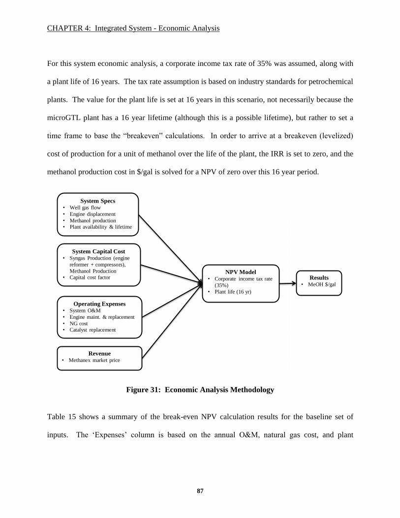
CHAPTER 4: Integrated System - Economic Analysis
87
For this system economic analysis, a corporate income tax rate of 35% was assumed, along with
a plant life of 16 years. The tax rate assumption is based on industry standards for petrochemical
plants. The value for the plant life is set at 16 years in this scenario, not necessarily because the
microGTL plant has a 16 year lifetime (although this is a possible lifetime), but rather to set a
time frame to base the “breakeven” calculations. In order to arrive at a breakeven (levelized)
cost of production for a unit of methanol over the life of the plant, the IRR is set to zero, and the
methanol production cost in $/gal is solved for a NPV of zero over this 16 year period.
Figure 31: Economic Analysis Methodology
Table 15 shows a summary of the break-even NPV calculation results for the baseline set of
inputs. The ‘Expenses’ column is based on the annual O&M, natural gas cost, and plant
System Specs• Well gas flow
• Engine displacement
• Methanol production
• Plant availability & lifetime
System Capital Cost• Syngas Production (engine
reformer + compressors),
Methanol Production
• Capital cost factor
Operating Expenses• System O&M
• Engine maint. & replacement
• NG cost• Catalyst replacement
Revenue• Methanex market price
NPV Model• Corporate income tax rate
(35%)
• Plant life (16 yr)
Results• MeOH $/gal

CHAPTER 4: Integrated System - Economic Analysis
88
refurbishment and is of the form: Annual O&M + Annual Natural Gas Cost + Refurbishment
(every 2 years). For example, in year 3 (Table 15), the ‘Expenses’ calculation is:
($6.03/bbl x 49 bbl/day x 0.8 x 365 day) + ($0.5/Mscf x 333,000 Mscf x 0.8 x 365)
+ ($10,000 catalyst + $53,900 engine) = $198,185.
(18)
The natural gas price in this baseline case is $0.50/Mscf (approx. $0.50/MMBtu).36
This natural
gas price is lower than the pipeline natural gas price (pipeline price at approximately $3/MMBtu
through most of 2015) based on the assumption that the natural gas that would otherwise be
flared at the well site is considered a wasted resource with little value.
The ‘revenue’ value in Table 15 represents the revenue generated from producing methanol at
the breakeven production cost. As mentioned above, this breakeven methanol production cost is
calculated by setting the IRR for the plant to zero and solving the NPV for zero at the end of the
designed plant life (16 years in this case).37
Under these conditions (IRR = 0, NPV solved for 0),
the “revenue” are the proceeds from selling the methanol at the break-even cost.38
The ‘Cash
Flow’ calculation in Table 15 includes the corporate income tax rate to arrive at the annual cash
flow. The equation for ‘Cash Flow’ is of the form: (1 – tax rate) x (Revenue – Expenses). For
example, in year 3 the calculation would be:
(1 – 0.35) x ($309,189 – 198,185) = $72,153 (19)
36 1 Mscf = 1.028 MMBtu. Within industry, these values are used interchangeably.
37 The Excel ‘solver’ function was used in the spreadsheet shown in Table 14 in section 4.4.1
38 The revenue for Year 1 is half that of the subsequent years, accounting for a 6 month period for the initial
production run of the mass-produced microGTL systems. This assumption is likely conservative compared to an n-
th unit economic analysis that likely wouldn’t need to consider a 6 month delay in deployment.

CHAPTER 4: Integrated System - Economic Analysis
89
The NPV values for each year in Table 15 represent the NPV for the system if it was discarded at
the end of that particular year. The NPV is zero for year 16 because that is the design life of the
plant. The NPV calculations prior to year 16 return a negative value because the plant would be
losing money if it were to shut down prior to the design lifetime.
Table 16 shows the methanol production cost results ($ per gallon of methanol) for a range of
natural gas prices for the microGTL system (‘Small Scale’ column). These values were obtained
by modifying the natural gas cost and holding the other system economic parameters constant.
The economic analysis methodology previously described was then applied to arrive at the new
methanol production cost. At a $0.50/Mscf natural gas price, the breakeven (levelized) cost of
production is $0.52/gallon of methanol. The ‘Large Scale’ column in Table 16 is based on
proprietary industry estimates for large-scale methanol production cost.39
At $0.50/Mscf and all
other economic factors at the baseline values as reviewed above for the microGTL system, the
methanol production cost of $0.52/gal compares with large-scale methanol production at
approximately $4.50/Mscf of natural gas (interpolating from Table 16).
39 Large-scale methanol production cost estimate provided by Vikram Rao, RTI.

CHAPTER 4: Integrated System - Economic Analysis
90
Table 15: Summary of NPV Calculations
Table 16: Methanol Production Cost
Year Expenses Revenue Cash Flow NPV
1 $134,285 $154,594 $13,201 ($1,414,568)
2 134,285 309,189 113,688 (1,300,880)
3 198,185 309,189 72,153 (1,228,728)
4 134,285 309,189 113,688 (1,115,040)
5 198,185 309,189 72,153 (1,042,888)
6 134,285 309,189 113,688 (929,200)
7 198,185 309,189 72,153 (857,048)
8 134,285 309,189 113,688 (743,360)
9 198,185 309,189 72,153 (671,208)
10 134,285 309,189 113,688 (557,520)
11 198,185 309,189 72,153 (485,368)
12 134,285 309,189 113,688 (371,680)
13 198,185 309,189 72,153 (299,528)
14 134,285 309,189 113,688 (185,840)
15 198,185 309,189 72,153 (113,688)
16 134,285 309,189 113,688 0
NG Price ($/Mscf) Small Scale Large Scale
$0.00 $0.43 $0.12
$0.50 $0.52 $0.16
$1.00 $0.60 $0.21
$2.00 $0.77 $0.30
$3.00 $0.95 $0.39
$4.00 $1.12 $0.48
$5.00 $1.29 $0.57
$6.00 $1.46 $0.66
Production Cost ($/gal)

CHAPTER 4: Integrated System - Economic Analysis
91
4.4.5 Sensitivity Analysis
A sensitivity study was performed using the economic model reviewed in this chapter. Five
factors from Table 14 (in red) were used for this sensitivity study; however the economic model
is structured to allow for sensitivity analyses for all of the system variables. The economic
factors considered for this sensitivity analysis are:
1. conversion efficiency (‘Methanol production’),
2. time on stream,
3. total plant capital cost,
4. refurbishment cost, and
5. natural gas cost.
For each factor, a range of values was evaluated, holding all other inputs in the economic
constant, to arrive at an alternate methanol production cost. Figure 32, a tornado chart, displays
the results from the sensitivity study for these five factors. The tornado chart allows for
straightforward visual comparisons of the sensitivity of various economic factors on the
methanol production cost on a single chart.
Starting from the baseline system capital cost estimate of $1.43mil, a 50% change to the capital
cost was used for the bounds of the sensitivity analysis. As Figure 32 shows, a 50% reduction in
capital cost reduces the methanol production cost by approximately $0.20/gal (from $0.52/gal to
$0.32/gal) – this is designated by the green bar to the left of the baseline in the tornado chart.
While an upper bound at $2.1mil was included, it is likely that the current capital cost estimate
($1.43mil) is conservative, and the n-th unit commercial scale system will have a lower capital

CHAPTER 4: Integrated System - Economic Analysis
92
cost than the baseline case presented here. One of the keys to lowering the capital cost will be to
lower the cost of the compressor system, whether this comes from a cheaper compressor
technology, or by requiring less compression. Any effort to reduce the compression requirement
will likely include reducing the N2 that is passed through the system, increasing the partial
pressures of the H2 and CO. A scenario with 95% O2 in the inlet feed gas was briefly reviewed
in section 4.3 to provide an estimate of the reduced system capital cost potential of an O2
enriched inlet stream. In a case where the overall mass flow is reduced, such as in the theoretical
95% O2 example, the methanol reactor system could likely be downscaled along with the sub-
components (i.e. heat exchangers, coolers, H2 membrane), further reducing the system size. Any
reductions in capital cost due to downsizing components would need to be considered together
with the increased expense incurred from whatever system is used to provide enriched O2.
Figure 32: Methanol Production Cost Sensitivity (Tornado Chart)

CHAPTER 4: Integrated System - Economic Analysis
93
The impact of natural gas cost on the methanol production cost is included in Figure 32 for a
range of natural gas cost from $0 to $1/Mscf. Table 16 includes a broader range of natural gas
prices related to the methanol production cost for the same set of economic conditions. The
results in Figure 32 show that a reduction in the natural gas cost from $0.50 to $0.00 reduces the
methanol production cost by approximately $0.09/gal. For context, this reduction in natural gas
cost is equivalent to a $300k reduction in system capital cost when comparing these results in the
tornado chart. If this system is successfully deployed, and/or if other groups are successful in
commercializing microGTL technologies aimed at utilizing and monetizing otherwise flared
natural gas, then it is likely that a market will be created for this resource, potentially reducing
the likelihood that “free” natural gas will be an option. It is reasonable to expect that the market
price for the flared gas will still sell at a steep discount to pipeline quality natural gas due to
number of issues, including the raw state of the gas, and the fact that it is delivered locally and at
reduced pressures than that of pipeline gas. Alternately, a zero or negative price for natural gas
could occur in circumstances where environmental regulations exist and using the microGTL
system is the cheapest solution to meeting these regulations.
The methanol reactor system conversion efficiency is 60% for the baseline case. The engine
reformer conversion of CH4 is high (99% of the CH4 is converted, mostly to CO, and some CO2),
so the total system conversion efficiency for CH4 to CH3OH (methanol) is dominated by the
performance of the methanol reactor system in converting the syngas-rich stream from the
engine reformer into methanol. The sensitivity to conversion efficiency is included here, but will
ultimately be determined based on the technical limitations of the system from Casale combined
with an internal economic analysis weighing the cost of the reactor system vs. conversion rate.

CHAPTER 4: Integrated System - Economic Analysis
94
Time on stream will be determined by the specific use cases for this microGTL system. For
example, in the case of associated gas (natural gas from shale oil development), the time on
stream could approach 100% over extended periods of time, with downtime for scheduled
maintenance. Due to the variable nature of associated gas flows in tight oil wells, the time on
stream could end up considerably lower than 100% if, for example, the associated gas flow is at
80% of the microGTL capacity for 80% of the time, resulting in an effective time on stream (or
capacity factor) of 64%. In the well-completion scenario (for shale gas and oil), it’s likely that
the time on stream would also approach 100% during the well-completion (typically 3 to 6
weeks), but may have more significant downtime as the system is moved from well to well.
Refurbishment cost (replacing worn out components of the system) is currently dominated by the
engine reformer replacement ($53,900 out of $63,900 total), with methanol reactor catalyst
replacement contributing approximately 15% to the overall refurbishment cost (the remaining
$10,000). While it is possible that catalyst contamination may require more frequent
replacement, the current economic model includes $90k (6.5% of capital cost) for contaminant
removal prior to the methanol reactor. The trade-off between costs for contaminant removal
systems vs. catalyst replacement will be reviewed in more detail for the commercial scale
system. It is likely that the bulk of the smaller system components will also require
refurbishment or replacement throughout the ‘plant’ lifetime. At this stage of the system design,
it is premature to assign detailed refurbishment costs for many of these components. In lieu of
these cost estimates, it is assumed that the 2x capital cost factor contributes to these
refurbishment costs for a theoretical n-th scale unit.

CHAPTER 4: Integrated System - Economic Analysis
95
The fact that engines are cheap and mass produced results in a low sensitivity of the overall
methanol production cost to the engine replacement schedule. This is visible in Figure 32. The
low cost of engines and engine replacements contributes significantly to the economic viability
of this microGTL system. In the following chapter, a more detailed economic analysis will
dissect the syngas production cost from the engine reformer system and compare this to the
syngas production cost from large-scale systems.

CHAPTER 5: Syngas Production - Economic Analysis
96
CHAPTER 5: Syngas Production - Economic Analysis 40
5.1 Introduction
In the previous chapter, the economic analysis for the commercial scale microGTL system was
reviewed, with the outcome of the analysis focused on the cost of methanol production, and a
comparison to the production cost for large-scale methanol production. Since the engine
reformer system is the novel component of this process and the primary contributor to the
economic viability of this system, this chapter presents a more nuanced economic study focused
on the production cost of the intermediate syngas, and compares this syngas production cost to
the cost of syngas production in large-scale systems. The comparison is made on a per-energy-
content basis to address the fact that the chemical compositions of the product streams are not
identical between the microGTL and large-scale systems. The syngas cost estimates for the
large-scale systems is transparent, unlike the large-scale methanol production cost in the
previous chapter, supporting a more robust comparison between systems. As the results will
show, the syngas production cost for this system compares favorably to large-scale centralized
syngas production. However, it should be noted that in the current design the engine reformer
40 The majority of the discussion and results in this chapter are from the journal submission “Economic analysis of a
non-catalytic, partial-oxidation methane reformer using an internal combustion engine.” This journal article was
authored by myself as 1st author, with John Carpenter (RTI), Raghubir Gupta (RTI), and Klaus Lackner
(ASU/Columbia) as co-authors.

CHAPTER 5: Syngas Production - Economic Analysis
97
produces a syngas that is mixed with a large fraction of nitrogen. This in effect lowers the value
of the product, but it also lowers costs.
5.2 Background
Economical syngas production typically takes place in large chemical processing facilities that
produce methanol, ammonia, and other products with methane as a feedstock. Increased natural
gas discoveries and extraction, mostly due to improvements in hydraulic fracturing and
horizontal drilling technologies, have created a market for distributed natural gas resources,
either as part of dry gas extraction or associated gas from oil extraction. These newfound
discoveries have contributed to an increased interest in small GTL development at varying scales
and with various end products. As mentioned in section 1.4.2, a 2014 report by the World Bank
summarized the status of 24 companies working to commercialize small GTL systems (Fleisch,
2014). Building on the World Bank study, a 2015 report by ADI Analytics, specifically focusing
on small-scale methanol production, identified the market potential for new technologies to take
advantage of recent shale gas discoveries. While this report highlights the economic potential
for small-scale methanol technologies, the report states that “Currently, no process technology
has been commercially proven for small-scale methanol plants” (ADI Analytics LLC, 2015).
The vast majority of the technologies reviewed in both the World Bank and ADI Analytics small
GTL reports assume that the syngas will be provided, and that the “GTL” technology is, in fact,
syngas-to-liquid. Currently, syngas production cannot be straightforwardly scaled down, as is

CHAPTER 5: Syngas Production - Economic Analysis
98
evidenced by the complete lack of small-scale syngas production systems in existence.41
This
detail highlights the difficulty in producing syngas at small and very-small scales. A key
element of this thesis is to address this shortcoming.
5.3 Large-scale Syngas Production Cost Baseline
The production cost for syngas from large-scale chemical processing facilities that use natural
gas as a feedstock was used as the baseline for comparison in this study. Results from four
published economic analyses were used to derive a range of baseline syngas production costs on
a per energy content basis in units of $/MMBtu (Choi, Kramer, Tam, & Fox, 1997; National
Energy Technology Laboratory, 2013; Noureldin, Elbashir, & El-Halwagi, 2014; Pei, Korom,
Ling, & Nasah, 2014). In two of these studies (Choi, et al. and NETL), the syngas production
cost was extracted from the overall cost of large-scale Fischer-Tropsch (F-T) facilities, and in the
other two studies (Noureldin, et al. and Pei, et al.), direct estimates for syngas production cost
were reported.
The system economic parameters of the National Energy Technology Laboratory (NETL) model
were used as the baseline for the cost estimates of the other systems. For the method used in this
economic analysis, small adjustments were made to the economic parameters for the other three
studies to obtain comparable syngas production costs. Ultimately, the small-scale syngas
production (based on the microGTL system) was scaled to the NETL system as well, and will be
discussed in this chapter.
41 Supported by written (email) communication with Vikram Rao, October, 2014.
CHAPTER 5: Syngas Production - Economic Analysis
99
A summary of the baseline economic parameters for each of the four studies in shown in Table
17 and will be reviewed in detail for each study in subsequent sections in this chapter. The
values in Table 17 are for each of the economic studies before adjustments to compare with the
NETL study, and are meant to show the similarities (and differences) between each of the four
studies. The Choi, et al. study is similar in scale to the NETL study, with the only differences
being the overall plant lifetime (33 years vs. 35 years, including construction). A discussion of
the sensitivity to changes in plant life will be discussed in section 5.3.1.1.
For the Pei et al. study, the “production life” of the plant was reported (30 years), but the
construction time was not discussed. For this analysis, the construction time was assumed to be
5 years (same as NETL) based on the fact that the production lifetime was the same as the NETL
study (30 years). The discount rate was also adjusted (from 9.1% to 7.4%). While the scale of
the syngas production in Pei et al. is about one-quarter the scale of the NETL (and Choi, et al.)
study in terms of inlet feedstock volume, it is still considered ‘large scale’ and was left as is for
this analysis. Alternatively, the Pei et al. system could have been scaled up from 102 MMscfd to
410 MMscfd of natural gas using a scaling law, but this would add another layer of assumptions
to the comparison. The production volumes for F-T liquids in these three studies varies based on
the process used for the syngas-to-liquid conversion. It is reported here, but not used in the
analysis.
Unlike the other three studies, Noureldin, et al. instead constructed a syngas production cost
based on the production costs for H2, CO, and O2. While the Noureldin, et al. method to estimate

CHAPTER 5: Syngas Production - Economic Analysis
100
syngas production cost claims to be “independent of operational scale,” the sources for the
feedstocks for the syngas production are taken from large-scale facilities.
Table 17: Baseline Large-Scale System economic parameters
NETL Choi Pei Noureldin
Construction (yr) 5 4 n/a n/a – “large-scale”
Production (yr) 30 29 30 n/a
Discount Rate (%) 7.4 7.4 9.1 n/a
Feedstock Scale (NG – MMscfd) 410 412 102 n/a
Production (bbl/day F-T liquid) 50,000 45,000 7,650 n/a
To obtain comparable syngas production cost between the four large-scale studies, a net present
value (NPV) calculation similar to the method from the previous chapter was used. In each case,
only the discount rate was normalized to the NETL system, with the other system parameters left
as is. The syngas production cost was then determined by solving for a NPV of zero over the
design life of the plant. The discount rate was set equal to the Internal Rate of Return (IRR) to
arrive at a break-even, or levelized cost. This method to determine the break-even cost is the
same method that was used in the previous chapter to arrive at the methanol production cost for
the integrated commercial scale system. In all cases, the costs were adjusted to 2014 dollars.
Figure 33 shows the process flow diagram from the NETL techno-economic analysis of a large-
scale F-T liquid facility. The pre-reformer and reformer inside the oval are included in the

CHAPTER 5: Syngas Production - Economic Analysis
101
subsystem economic analysis used to derive the syngas production cost for the large-scale
systems. In all cases, the cost basis for the system capital cost, fixed O&M, and variable O&M
were scaled to 2014 $ using the U.S. Bureau of Labor Statistics Producer Price Index (PPI) for
processed fuels for intermediate demand (United States Bureau of Labor Statistics, 2015).42
A
fixed natural gas price of $3/MMBtu was used in all cases, including the small-scale case. This
differs from the economic analysis for the microGTL system in the previous chapter due to the
fact that large-scale petrochemical facilities pay market price for industrial scale pipeline natural
gas, and do not have access to stranded natural gas. A syngas production cost with a reduced
natural gas cost is included in a sensitivity study in this chapter.
42 Refer to section 5.5.1 for a brief discussion on the Producer Price Index.

CHAPTER 5: Syngas Production - Economic Analysis
102
Figure 33: Process Flow Diagram for 50,000 bbl/day F-T system
(National Energy Technology Laboratory, 2013)
5.3.1 Large-scale Syngas Production Cost Calculations
Economic analyses from four large-scale Natural-Gas-to-Fischer-Tropsch-Liquids systems were
used to arrive at a range of baseline values for large-scale syngas production cost. A summary of
the methods and results for each of the four large-scale systems is presented here.

CHAPTER 5: Syngas Production - Economic Analysis
103
5.3.1.1 “Design and economics of a Fischer-Tropsch plant for converting natural gas to
liquid transportation fuels,” (Choi et al., 1997)
The Choi, et al. report, funded by the DOE (DE-AC22-91PC90027) and carried out by Bechtel
and Amoco, reviewed the economics for an advanced F-T plant using coal and natural gas as
feedstocks. The economic results from the natural-gas-based system were used to arrive at the
large-scale syngas production cost baseline for this particular study. Table 18, from Choi, et al.,
summarizes the system input and output flows, as well as the cost breakdown of the major
components of the plant and the economic parameters used in the economic analysis used in this
report. The values from Table 18 were used to feed the inputs in Table 19 for the economic
analysis in the syngas cost comparison study. In addition to the unit conversions for the input
and output flows and economic parameters, the percentage of the overall plant capital cost due to
syngas production was taken from Table 18 and used to derive the results presented in Table 19
($707 / $1,842 = 38.38%). Additional economic inputs necessary for the comparison to the other
systems in this study are also included in Table 19 (NG cost, O&M). The cost basis was also
adjusted to 2014$.
The system capital cost ($1,737,436,399), O&M costs (converted from $/bbl to $), and feedstock
(natural gas) cost from the results of the Table 19 calculations were used as inputs into the NPV
model in Table 20. The discount rate (7.4%) was based on the interest rate (8%) as stated in
Choi et al. Recognizing that the discount rate is used to calculate the present value of future cash
flows, the discount rate can be related to the interest rate by the equation:
d = 1 – 1/(1+r) (20)

CHAPTER 5: Syngas Production - Economic Analysis
104
where ‘d’ is the discount rate and ‘r’ is the interest rate. The 8% interest rate is also the value
used in the NETL report. Solving the NPV column for zero over the lifetime of the plant
resulted in the syngas production cost for this system of $5.42/MMBtu.

CHAPTER 5: Syngas Production - Economic Analysis
105
Table 18: Economic factors for Choi, et al.
Source: (Choi et al., 1997)

CHAPTER 5: Syngas Production - Economic Analysis
106
Table 19: Economic Analysis Calculations for Choi, et al.
Estimate Syngas cost
Inlet:
NG 412 MMSCF/day
NG 17,800 MMBTU/hr
NG 427200 MMBTU/day
N-Butane 340 bbl/day
N-Butane 1496 MMBTU/day
Total 428696 MMBTU/day
Outlet:
Gasoline 17,000 bbl/day
Gasoline 86700 MMBTU/day
Diesel 26200 bbl/day
Diesel 150781 MMBTU/day
Propane 1700 bbl/day
Propane 6521.2 MMBTU/day
Electricity 592 MWh/day
Electricity 2019.904 MMBTU/day
Total 246022.104 MMBTU/day
Total 44,900 bbl/day
NETL Syngas eff 83.40%
ideal ATR eff 88.36%
Syngas (est.) 357526.3207 MMBTU/day
Syngas (est.) 2962284331 MMBTU total life of plant
Syngas Cap cost 707000000 $ (1993)
Syngas Cap cost $1,737,436,339 $ (2014)
Syngas % of total 38.38%
NG cost 3 $/MMBTU
NG cost $424,747,872 $/yr
NG Total 3539565600 MMBTU total life of plant
NG Total $10,618,696,800 $
Cap + NG $12,356,133,139 $
Syngas 4.17 $/MMBTU
EIA NG FT Liquids O&M
Fixed 10.37 $/bbl
Variable 48.36 $/bbl includes feedstock
Total 58.73 $/bbl
Total $873,946,917 $
Total minus NG $449,199,045 $
Total for Syngas $172,412,446 $ 2011 $
Total for Syngas $166,981,133 $ 2014 $

CHAPTER 5: Syngas Production - Economic Analysis
107
Table 20: NPV Calculations for Choi, et al.
Total Construction Cost 1,737,436,339$ 2014 $/MMBTU:
Fixed + Variable O&M Cost 166,981,133$ $5.42
Annual Fuel Cost 424,747,872$
Engine Replacement Cost -$
Plant Replacement Cost -$
Total Future Annual Benefits: $762,010,074
Year Annual Cash Flow (Costs) ($) Discount Rate NPV ($)
2015 (434,359,085)$ 7.41% -$434,359,085
2016 (434,359,085)$ 7.41% -$404,403,286
2017 (434,359,085)$ 7.41% -$376,513,404
2018 (434,359,085)$ 7.41% -$350,546,962
2019 170,281,069$ 7.41% $127,946,802
2020 170,281,069$ 7.41% $119,122,884
2021 170,281,069$ 7.41% $110,907,513
2022 170,281,069$ 7.41% $103,258,719
2023 170,281,069$ 7.41% $96,137,428
2024 170,281,069$ 7.41% $89,507,260
2025 170,281,069$ 7.41% $83,334,346
2026 170,281,069$ 7.41% $77,587,150
2027 170,281,069$ 7.41% $72,236,312
2028 170,281,069$ 7.41% $67,254,497
2029 170,281,069$ 7.41% $62,616,256
2030 170,281,069$ 7.41% $58,297,893
2031 170,281,069$ 7.41% $54,277,349
2032 170,281,069$ 7.41% $50,534,084
2033 170,281,069$ 7.41% $47,048,974
2034 170,281,069$ 7.41% $43,804,218
2035 170,281,069$ 7.41% $40,783,237
2036 170,281,069$ 7.41% $37,970,600
2037 170,281,069$ 7.41% $35,351,938
2038 170,281,069$ 7.41% $32,913,873
2039 170,281,069$ 7.41% $30,643,951
2040 170,281,069$ 7.41% $28,530,575
2041 170,281,069$ 7.41% $26,562,949
2042 170,281,069$ 7.41% $24,731,022
2043 170,281,069$ 7.41% $23,025,434
2044 170,281,069$ 7.41% $21,437,473
2,689,871,462$ $0
Costs
Revenue required for breakeven production cost

CHAPTER 5: Syngas Production - Economic Analysis
108
5.3.1.2 “Cost comparison of syngas production from natural gas conversion and
underground coal gasification,” (Pei et al., 2014)
This recent study (Pei et al., 2014) by the University of North Dakota compares syngas
production costs for coal and natural gas systems, similar to the Choi, et al. report discussed in
the previous section. Unlike the NETL and Choi, et al. reports however, the syngas production
cost is explicitly stated in this report based on a set of economic assumptions. The economic
model presented in this economic analysis was dissected and the syngas production cost was
recalculated using the parameters from the NETL system. This study reports a “production
lifetime” for the plant at 30 years (same as the production lifetime for the NETL system), but
does not include construction time. A construction time of 5 years was assumed for this analysis
to allow for a direct comparison to the NETL system. The interest rate (and corresponding
discount rate) was adjusted from 10% to 8% to align with the economics of the NETL system as
well.
Table 21 and Table 22 are taken directly from Pei, et al. The GTL plant assumptions stated in
Table 21were used to calculated the construction cost and O&M for the syngas production. The
‘Total Construction Cost’ used in
Table 23 was based on the capital cost and ‘Fraction of syngas production in capital investment’
from Table 21. The percentage of the overall plant capital cost attributed to syngas production
was then adjusted from 2012 $ to 2014 $ to arrive at the value in
Table 23. The calculation is as follows:
60% x $210,000/m3/d x 1,216 m
3/d x 0.97 = $149,600,000 (21)

CHAPTER 5: Syngas Production - Economic Analysis
109
The Producer Price Index for 2014 was lower than for 2012. A factor of 0.97 was used in
equation (21) to convert the capital cost to 2014 $.
Table 23 shows the results from the economic model used to arrive at the syngas production cost
with the NPV set to zero for the designed plant life. This method was validated first by
reproducing the result from Table 22 for a $3/MMBtu natural gas price ($112.09/TCM), and then
recalculated with the updated (NETL) economic parameters (i.e. change to the discount rate).
Solving the NPV column for zero over the lifetime of the plant resulted in the syngas production
cost for this system of $5.02/MMBtu.
Table 21: GTL Plant Assumptions for Pei et al.
Source: (Pei et al., 2014)

CHAPTER 5: Syngas Production - Economic Analysis
110
Table 22: Syngas Production Cost vs. Natural Gas Price for Pei et al.
‘TCM’: thousand cubic meter
Source: (Pei et al., 2014)

CHAPTER 5: Syngas Production - Economic Analysis
111
Table 23: NPV Calculations for Pei, et al.
$/TCM @ r = 10%:
Total Construction Cost 149,600,919$ $63.03
Fixed + Variable O&M Cost 10,920,867$
Annual Fuel Cost 118,142,860$ $/TCM:
Engine Replacement Cost -$ $60.50
Plant Replacement Cost -$
2014 $/MMBTU:
$5.02
Total Future Annual Benefits: $143,487,178
Year Annual Cash Flow (Costs) ($) Discount Rate NPV ($)
2015 (29,920,184)$ 7.41% -$29,920,184
2016 (29,920,184)$ 7.41% -$27,856,723
2017 (29,920,184)$ 7.41% -$25,935,570
2018 (29,920,184)$ 7.41% -$24,146,910
2019 (29,920,184)$ 7.41% -$22,481,605
2020 14,423,451$ 7.41% $10,090,159
2021 14,423,451$ 7.41% $9,394,286
2022 14,423,451$ 7.41% $8,746,404
2023 14,423,451$ 7.41% $8,143,204
2024 14,423,451$ 7.41% $7,581,604
2025 14,423,451$ 7.41% $7,058,735
2026 14,423,451$ 7.41% $6,571,925
2027 14,423,451$ 7.41% $6,118,689
2028 14,423,451$ 7.41% $5,696,711
2029 14,423,451$ 7.41% $5,303,834
2030 14,423,451$ 7.41% $4,938,052
2031 14,423,451$ 7.41% $4,597,497
2032 14,423,451$ 7.41% $4,280,428
2033 14,423,451$ 7.41% $3,985,226
2034 14,423,451$ 7.41% $3,710,383
2035 14,423,451$ 7.41% $3,454,495
2036 14,423,451$ 7.41% $3,216,254
2037 14,423,451$ 7.41% $2,994,443
2038 14,423,451$ 7.41% $2,787,930
2039 14,423,451$ 7.41% $2,595,659
2040 14,423,451$ 7.41% $2,416,648
2041 14,423,451$ 7.41% $2,249,982
2042 14,423,451$ 7.41% $2,094,811
2043 14,423,451$ 7.41% $1,950,341
2044 14,423,451$ 7.41% $1,815,835
2045 14,423,451$ 7.41% $1,690,605
2046 14,423,451$ 7.41% $1,574,012
2047 14,423,451$ 7.41% $1,465,459
2048 14,423,451$ 7.41% $1,364,393
2049 14,423,451$ 7.41% $1,270,297
2050 14,423,451$ 7.41% $1,182,690
297,526,068$ $0
Costs
Revenue required for breakeven production cost

CHAPTER 5: Syngas Production - Economic Analysis
112
5.3.1.3 “Optimization and selection of reforming approaches for syngas generation from
natural/shale gas.” (Noureldin et al., 2014)
Another recent study, Noureldin et al., 2014, looked at several different reforming approaches
from natural gas. This particular study developed an “economic potential” metric to compare
various methods of syngas production based on revenue, raw material cost, and energy cost.
Noureldin, et al. claimed that this “economic potential” metric was “independent of operation
scale” (Noureldin et al., 2014). However, this method used production costs for H2, CO, and O2
from large-scale sources as raw material inputs to the economic model. While Noureldin et al.
does not offer more detail, they discuss two recently constructed GTL plants, the Shell Pearl
GTL and Sasol Oryx GTL, both located in Qatar, producing 260,000 bbl/day and 34,000 bbl/day
of a range of liquid petroleum products, respectively. The Shell Pearl GTL is the largest in the
world, and produces both petroleum liquids (140,000 bbl/day) and natural gas liquids (NGL,
120,000 bbl/day equivalent).
Table 24 is taken from the Noureldin, et al. study, and Table 25 shows the simple calculations
used to arrive at the syngas production cost of $5.89/MMBtu for the H2:CO ratio used in this
study. Unlike the other large-scale systems evaluated in this study, the Noureldin et al. report
did not provide enough economic information about the overall system to allow for a more
detailed economic analysis. Due to the relatively insufficient data compared to the other large-
scale studies reviewed here, this study should be considered as a complement to the other three
large-scale F-T system economic analyses.

CHAPTER 5: Syngas Production - Economic Analysis
113
Table 24: H2:CO Ratio vs. Syngas Price for Noureldin, et al.
Source: (Noureldin et al., 2014)
Table 25: Syngas cost for H2:CO = 2.0 for Noureldin, et al.
Convert $0.15/kg syngas to $/MMBTU
Based on $3/MMBTU NG
syngas heat of combustion: 285.08 kJ/mol
syngas heat of combustion: 270.21 btu/mol
syngas molar mass: 10.68 g/mol
$0.15/kg: 5.93 $/MMBTU (2013 $)*
5.89 $/MMBTU (2014 $)
* assumed - cost basis not stated in report
L/mol (22.4 vs. 24.789 for 0deg and 25deg, respectively)
Currently using 0deg value (22.4L/mol)

CHAPTER 5: Syngas Production - Economic Analysis
114
5.3.1.4 “Analysis of Natural Gas-to Liquid Transportation Fuels via Fischer-Tropsch.”
(National Energy Technology Laboratory, 2013)
This NETL study was used as the basis for comparison to the other large-scale systems as well as
the small-scale engine reformer system. This recent study transparently presents a thorough
techno-economic analysis of a state-of-the-art F-T system with natural gas as the feedstock.
Table 26 summarizes the pertinent system and economic inputs for the NPV calculations for the
NETL system. The inlet conditions and stream flow data are taken directly from the NETL
report, with units conversions where necessary to align with the format of this economic
analysis. The stream flow outlet is for the intermediate syngas step represented by the ‘Syngas’
stream in Figure 33. Using the economic data from the NETL report, the capital cost for the
syngas production ($1,029.011.000) was extracted from the overall F-T system capital cost. This
capital cost includes the air separation unit ($299,725,000), pre-reformer ($322,704,000), and
reformer ($406,582,000). The pipeline natural gas is delivered at pressure (31 bar), so there is no
compressor unit included in the syngas production cost.
The ratio of the capital cost for the syngas production to the overall F-T plant capital cost was
used to estimate the fraction of the stated overall F-T system fixed and variable O&M to syngas
production fixed and variable O&M. For example, the syngas fixed O&M calculation is:
‘Total System Fixed O&M’ ($/yr) x ‘Ratio of syngas to system cap cost’ / syngas
MMBtu/yr = Syngas Fixed O&M ($/MMBtu)
(22)
Referencing the values in Table 26, the result is:
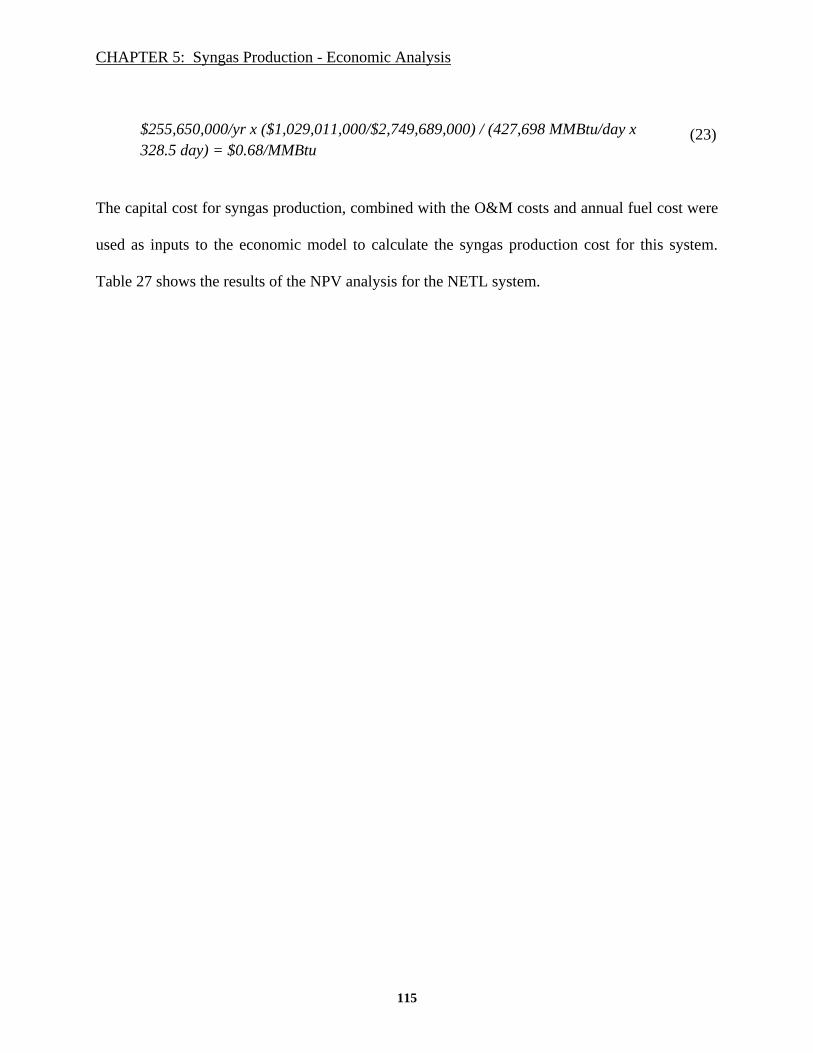
CHAPTER 5: Syngas Production - Economic Analysis
115
$255,650,000/yr x ($1,029,011,000/$2,749,689,000) / (427,698 MMBtu/day x
328.5 day) = $0.68/MMBtu (23)
The capital cost for syngas production, combined with the O&M costs and annual fuel cost were
used as inputs to the economic model to calculate the syngas production cost for this system.
Table 27 shows the results of the NPV analysis for the NETL system.
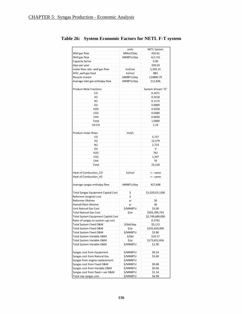
CHAPTER 5: Syngas Production - Economic Analysis
116
Table 26: System Economic Factors for NETL F-T system
units NETL System
Well gas flow MMscf/day 410.61
Well gas flow MMBTU/day 423,745
Capacity factor 0.90
days per year 328.50
molar flow rate -well gas flow mol/sec 5,503.31
HHV_well gas feed kJ/mol 883
Recycle stream MMBTU/day 114890.79
Average inlet gas enthalpy flow MMBTU/day 512,836
Product Mole Fractions System Stream "6"
CO 0.2471
H2 0.5418
N2 0.1173
O2 0.0000
H2O 0.0328
CO2 0.0580
CH4 0.0030
Total 1.0000
H2:CO 2.19
Product molar flows mol/s
CO 5,737
H2 12,579
N2 2,723
O2 0
H2O 762
CO2 1,347
CH4 70
Total 23,218
Heat of Combustion_CO kJ/mol <-- same
Heat of Combustion_H2 <-- same
Average syngas enthalpy flow MMBTU/day 427,698
Total Syngas Equipment Capital Cost $ $1,029,011,000
Reformer (engine) cost $ -
Reformer lifetime yr 30
Overall Plant lifetime yr 30
Unit Natural Gas Cost $/MMBTU $3.00
Total Natural Gas Cost $/yr $505,399,743
Total System Equipment Capital Cost $2,749,689,000
Ratio of syngas to system cap cost 0.3742
Total System Fixed O&M $/bbl/day $5,113
Total System Fixed O&M $/yr $255,650,000
Total System Fixed O&M $/MMBTU $2.80
Total System Variable O&M $/bbl $10.57
Total System Variable O&M $/yr $173,652,656
Total System Variable O&M $/MMBTU $1.90
Syngas cost from Equipment $/MMBTU $0.24
Syngas cost from Natural Gas $/MMBTU $3.60
Syngas from engine replacement $/MMBTU
Syngas cost from Fixed O&M $/MMBTU $0.68
Syngas cost from Variable O&M $/MMBTU $0.46
Syngas cost from fixed + var O&M $/MMBTU $1.14
Total raw syngas cost $/MMBTU $4.98

CHAPTER 5: Syngas Production - Economic Analysis
117
Table 27: NPV Calculations for NETL F-T System
Total Construction Cost 996,595,240$ 2014 $/MMBTU:
Fixed + Variable O&M Cost 155,596,136$ $5.39
Annual Fuel Cost 505,399,743$
Engine Replacement Cost -$
Plant Replacement Cost -$
Total Future Annual Benefits: $757,080,468
Year Annual Cash Flow (Costs) ($) Discount Rate NPV ($)
2015 -$199,319,048 7.41% -$199,319,048
2016 -$199,319,048 7.41% -$185,572,907
2017 -$199,319,048 7.41% -$172,774,775
2018 -$199,319,048 7.41% -$160,859,273
2019 -$199,319,048 7.41% -$149,765,530
2020 $96,084,589 7.41% $67,217,533
2021 $96,084,589 7.41% $62,581,841
2022 $96,084,589 7.41% $58,265,852
2023 $96,084,589 7.41% $54,247,517
2024 $96,084,589 7.41% $50,506,309
2025 $96,084,589 7.41% $47,023,115
2026 $96,084,589 7.41% $43,780,142
2027 $96,084,589 7.41% $40,760,822
2028 $96,084,589 7.41% $37,949,731
2029 $96,084,589 7.41% $35,332,508
2030 $96,084,589 7.41% $32,895,783
2031 $96,084,589 7.41% $30,627,109
2032 $96,084,589 7.41% $28,514,894
2033 $96,084,589 7.41% $26,548,350
2034 $96,084,589 7.41% $24,717,429
2035 $96,084,589 7.41% $23,012,779
2036 $96,084,589 7.41% $21,425,691
2037 $96,084,589 7.41% $19,948,057
2038 $96,084,589 7.41% $18,572,329
2039 $96,084,589 7.41% $17,291,478
2040 $96,084,589 7.41% $16,098,963
2041 $96,084,589 7.41% $14,988,689
2042 $96,084,589 7.41% $13,954,987
2043 $96,084,589 7.41% $12,992,574
2044 $96,084,589 7.41% $12,096,534
2045 $96,084,589 7.41% $11,262,290
2046 $96,084,589 7.41% $10,485,581
2047 $96,084,589 7.41% $9,762,437
2048 $96,084,589 7.41% $9,089,166
2049 $96,084,589 7.41% $8,462,327
2050 $96,084,589 7.41% $7,878,718
$1,982,027,021 $0
Costs
Revenue required for breakeven production cost

CHAPTER 5: Syngas Production - Economic Analysis
118
The results from all four large-scale systems are summarized in Table 28 and collectively
provide a range for the large-scale syngas production cost baseline.
Table 28: Baseline Syngas Production Cost, 2014$/MMBtu
5.4 Small-scale Syngas Production Cost Estimate
5.4.1 Integrated System Overview
Figure 34 shows a block diagram of the integrated microGTL system with the engine reformer.
The focus of this particular economic analysis will be the subsystem containing the engine
reformer and syngas compression steps. Figure 35 provides a more detailed depiction of the
components from the microGTL system that were considered as part of the syngas production
cost reported in this analysis.
Figure 34: Block Diagram for Engine Reformer (Small-Scale) GTL System
Syngas Production Cost - Baseline
Cost Basis - 2014 $
Source $/MMBtu
Pei, et al. $5.02
NETL $5.39
Choi, et al. $5.42
Noureldin, et al. $5.89

CHAPTER 5: Syngas Production - Economic Analysis
119
Figure 35: Aspen Process Flow Diagram
Components within the ovals are included in the syngas production cost estimate
5.4.2 Engine Reformer Syngas Production Cost
To calculate the syngas production cost for the small-scale engine reformer, the methodology
used to determine the large-scale syngas production cost based on the NETL system in Section
5.3 was used for this economic analysis as well. In addition to the economic parameter inputs
for the economic model, two technical factors must be considered as well. First, in the large-
scale production systems, it is assumed that the inlet natural gas feed from the distribution
pipeline is already at increased pressure (the NETL example received natural gas at 31 bar). In
the engine reformer system, it is assumed that the wellhead gas is close to atmospheric pressure,
which requires external gas compression to be included as part of the system process. In many
instances, wellhead natural gas may exit the well at pressures higher than 1 atmosphere, making
this a conservative assumption in some cases. The modular nature of the integrated microGTL
system will allow compression requirements to be modified to accommodate particular wellhead

CHAPTER 5: Syngas Production - Economic Analysis
120
characteristics (i.e. pressure, gas composition). Secondly, the engine lifetime for the mechanical
parts is significantly shorter than the lifetime of stationary reaction vessels and must be explicitly
considered. In the engine reformer system, it is assumed that the engine is replaced every other
year over the 35 year plant lifetime. For this study, it is also assumed that the entire system is
replaced at the half-way point of the 35 year plant life. This total system replacement is included
so that the economic comparison to the 35-year lifetime NETL plant can be performed.
With these economic assumptions considered, a syngas production cost estimate for the engine
reformer system can be calculated. Table 29 shows the economic factors used for the syngas
production cost estimate for the engine reformer system. The values for the NETL system from
Table 26 are included as well to straightforwardly compare the difference in scale between the
two systems in terms of these economic factors. The well gas flow for the small-scale system is
the same as has been discussed throughout this thesis (0.33 MMscfd). The time-on-stream is
adjusted to 0.90 to match the NETL system. The product stream data is taken from the Aspen
model data from Table 4 in section 3.1.3 (stream #12). The value for ‘Total Syngas Equipment
Capital Cost’ ($882,669) is taken from the microGTL system capital cost (Table 13 in section
4.3.1), and includes all of the components in the ‘Pre-conditioning’ step (cooler + water
separator, contaminant removal, and compressor system), and an additional cooler ahead of the
methanol reactor. The engine reformer cost is considered separately from the capital cost in this
analysis, as it is consumed every two years, unlike the remainder of the syngas production
system which is only replaced once over the 35 year plant life.

CHAPTER 5: Syngas Production - Economic Analysis
121
To estimate the O&M for the syngas production for the engine reformer system, the method
described in 4.4.3 for the overall O&M for the microGTL system was applied here, and scaled to
consider only the capital cost for syngas production. Using this method, 6% of the capital cost
for syngas production was used to derive the O&M cost.
Table 30 shows the results for the NPV analysis for this system. With $3/MMBtu as the natural
gas cost (the same as the large-scale systems), the syngas production cost for the small-scale
engine reformer system is $5.32/MMBtu. Figure 36 includes this result along with the range of
large-scale baseline cost estimates from Table 28. These initial results are encouraging and
potentially significant, as the estimated syngas production cost for the engine reformer system is
in-line with large-scale estimates under similar economic conditions. It should be noted that
while this result is on a per-Btu basis for H2 and CO, this comparison is not entirely fair because
the syngas from the microGTL system also contains a large amount of N2 that the large-scale
producers avoid.

CHAPTER 5: Syngas Production - Economic Analysis
122
Table 29: System Economic Factors for Engine Reformer System
units Engine Reformer System NETL System
Well gas flow MMscf/day 0.33 410.61
Well gas flow MMBTU/day 343.66 423,745
Capacity factor 0.90 0.90
days per year 328.50 328.50
molar flow rate -well gas flow mol/sec 4.46 5,503.31
HHV_well gas feed kJ/mol 883 883
Recycle stream MMBTU/day 114890.79
Average inlet gas enthalpy flow MMBTU/day 323 512,836
Product Mole Fractions "SynGas" stream System Stream "6"
CO 0.1116 0.2471
H2 0.2054 0.5418
N2 0.5302 0.1173
O2 0.0025 0.0000
H2O 0.1312 0.0328
CO2 0.0179 0.0580
CH4 0.0012 0.0030
Total 1.0000 1.0000
H2:CO 1.84 2.19
Product molar flows mol/s
CO 3.63 5,737
H2 6.68 12,579
N2 17.24 2,723
O2 0.08 0
H2O 4.26 762
CO2 0.58 1,347
CH4 0.04 70
Total 32.51 23,218
Heat of Combustion_CO kJ/mol 283.25 <-- same
Heat of Combustion_H2 286.00 <-- same
Average syngas enthalpy flow MMBTU/day 241 427,698
Total Syngas Equipment Capital Cost $ $882,669 $1,029,011,000
Reformer (engine) cost $ $53,900 -
Reformer lifetime yr 2 30
Overall Plant lifetime yr 18 30
Unit Natural Gas Cost $/MMBTU $3.00 $3.00
Total Natural Gas Cost $/yr $318,053 $505,399,743
Total System Equipment Capital Cost $1,427,769 $2,749,689,000
Ratio of syngas to system cap cost 0.6560 0.3742
Total System Fixed O&M $/bbl/day $5,113
Total System Fixed O&M $/yr $255,650,000
Total System Fixed O&M $/MMBTU $2.80
Total System Variable O&M $/bbl $10.57
Total System Variable O&M $/yr $173,652,656
Total System Variable O&M $/MMBTU $1.90
Syngas cost from Equipment $/MMBTU $5.59 $0.24
Syngas cost from Natural Gas $/MMBTU $4.02 $3.60
Syngas from engine replacement $/MMBTU $0.34
Syngas cost from Fixed O&M $/MMBTU $0.68
Syngas cost from Variable O&M $/MMBTU $0.46
Syngas cost from fixed + var O&M $/MMBTU $0.71 $1.14
Total raw syngas cost $/MMBTU $10.66 $4.98

CHAPTER 5: Syngas Production - Economic Analysis
123
Table 30: NPV Calculations for Small-Scale Engine Reformer System
Total Construction Cost 882,669$ $/MMBTU:
Fixed + Variable O&M Cost 56,194$ $5.32
Annual Fuel Cost 318,053$
Engine Replacement Cost 53,900$ Replace in odd years
Plant Replacement Cost 882,669$ Replace in year 19
Total Future Annual Benefits: $420,653
Year Annual Cash Flow (Costs) ($) Discount Rate NPV ($)
2015 -$882,669 7.41% -$882,669
2016 -$7,494 7.41% -$6,977
2017 $46,406 7.41% $40,226
2018 -$7,494 7.41% -$6,048
2019 $46,406 7.41% $34,869
2020 -$7,494 7.41% -$5,242
2021 $46,406 7.41% $30,225
2022 -$7,494 7.41% -$4,544
2023 $46,406 7.41% $26,200
2024 -$7,494 7.41% -$3,939
2025 $46,406 7.41% $22,711
2026 -$7,494 7.41% -$3,414
2027 $46,406 7.41% $19,686
2028 -$7,494 7.41% -$2,960
2029 $46,406 7.41% $17,065
2030 -$7,494 7.41% -$2,566
2031 $46,406 7.41% $14,792
2032 -$7,494 7.41% -$2,224
2033 $46,406 7.41% $12,822
2034 -$890,163 7.41% -$228,991
2035 $46,406 7.41% $11,115
2036 -$7,494 7.41% -$1,671
2037 $46,406 7.41% $9,634
2038 -$7,494 7.41% -$1,448
2039 $46,406 7.41% $8,351
2040 -$7,494 7.41% -$1,256
2041 $46,406 7.41% $7,239
2042 -$7,494 7.41% -$1,088
2043 $46,406 7.41% $6,275
2044 -$7,494 7.41% -$943
2045 $46,406 7.41% $5,439
2046 -$7,494 7.41% -$818
2047 $46,406 7.41% $4,715
2048 -$7,494 7.41% -$709
2049 $46,406 7.41% $4,087
2050 -$7,494 7.41% -$614
$0
Costs
Revenue required for breakeven production cost

CHAPTER 5: Syngas Production - Economic Analysis
124
Figure 36: Syngas Production Cost Comparison
5.5 Sensitivity Study
A sensitivity study was performed to understand the impact of three key variables - capital cost,
operating cost, and natural gas cost - on the cost of syngas production for the small-scale engine
reformer. The results from this sensitivity study are displayed in Figure 37.
To study the sensitivity of capital cost on syngas production cost, a range of capital costs
(CAPEX) 50% higher and 50% lower than the baseline were investigated. A lower capital cost
is envisioned by reducing the compressor cost (the dominant component in terms of capital cost
for syngas production) based on the potential to use the engine reformer to contribute to the
overall system compression requirements through inlet supercharging and modifications to the
valve train to utilize part of the high pressures seen within the combustion chamber.

CHAPTER 5: Syngas Production - Economic Analysis
125
Alternatively, compression requirements could be reduced by reducing the N2 that is passed
through the system, as discussed in the section 4.3.5 (95% O2 example). While reducing the
capital cost is always desirable, the results in Figure 37 (and Table 31) show that the syngas
production cost over the lifetime of the plant (35 years) is relatively insensitive to changes to
capital cost when compared to the other factors evaluated in the sensitivity study.
Similarly, the impact of operating cost (OPEX) sensitivity was evaluated by increasing and
decreasing the operating cost by 50%. These adjustments to the operating cost consider
changing the rate of engine replacement from every two years to every year or every third year
respectively over the system lifetime. Due to the relatively inexpensive engine, increasing the
replacement cost from every two years to every year (+50% OPEX in Figure 37) did not have a
significant impact on the overall syngas production cost.
Finally, reduced natural gas feedstock cost was selected as a sensitivity factor. As may have
been expected, these results show that the overall syngas production cost is dominated by the
natural gas feedstock cost. This is compelling, as an intended application for this microGTL
system is to address otherwise flared natural gas at well locations, where the natural gas
feedstock cost may be significantly less than pipeline natural gas. It is tempting to assume that
stranded natural gas has no cost, or that there is even a service charge for taking it away,
however once a market is created for this resource, then it is likely that $0/MMBtu may not be
realistic, but it is reasonable to assume that this resource will sell at a discount to pipeline natural
gas.

CHAPTER 5: Syngas Production - Economic Analysis
126
Figure 37: Syngas Production Cost Sensitivity Study for Engine Reformer System
Baseline case ($5.32 / MMBtu) designated by dashed line; 2014$ cost basis
Table 31: Data for Syngas Production Cost Sensitivity Study
5.5.1 Note on the cost basis used in this study
The United States Department of Labor Producer Price Index was used for the cost basis
calculations, and 2014 was used as the cost basis year. Figure 38 displays the annual PPI data
from 1990 to 2014. Specifically, the monthly data averaged to annual values for the “Processed
fuels and lubricants for intermediate demand” were used (United States Bureau of Labor
+50% OPEX +50% CAPEX -50% CAPEX -50% OPEX $1.50/MMBTU $0.00/MMBTU Baseline
Syngas CAPEX $ $882,669 $1,324,004 $441,335 $882,669 $882,669 $882,669 $882,669
Syngas OPEX $ $165,141 $110,094 $110,094 $55,047 $706,336 $110,094 $110,094
Natural Gas $/MMBTU $3.00 $3.00 $3.00 $3.00 $1.50 $0.00 $3.00
Syngas Cost $/MMBTU $5.86 $5.44 $5.21 $4.79 3.31 $1.30 $5.32

CHAPTER 5: Syngas Production - Economic Analysis
127
Statistics, 2015). As the data in Figure 38 shows, a slight downward trend in the PPI is observed
from 2011 through 2014. While this trend does not change the overall findings in this study, it is
worth mentioning that if/when the PPI regains a positive slope that the results from this study
could change slightly, as several of the economic analyses in this study were based on initial
costs in the 2011-2013 range.
Figure 38: Producer Price Index - Processed Fuels for Intermediate Demand
Source: U.S. Dept. of Labor

CHAPTER 6: Life Cycle Analysis
128
CHAPTER 6: Life Cycle Analysis
6.1 Overview
A life cycle analysis (LCA) was performed to evaluate the greenhouse gas emissions (GHG) for
a unit of methanol produced from the engine reformer microGTL system. The outcome of this
analysis compares the life-cycle GHG emissions from the microGTL system to the emissions
from a large-scale methanol plant. The comparison juxtaposes methanol production from
otherwise flared natural gas at a shale-gas well-site using the microGTL system to methanol
production from a large-scale plant that is delivered pipelined methane. A range of natural gas
system methane leakage values, transport distances, and methanol conversion efficiencies are
included as part of a sensitivity analysis.
6.2 Method
The functional unit for this LCA is 1 MMBtu of methanol produced. The analysis focuses on the
production and transport of liquid methanol from fossil sources, and does not consider the GHG
emissions associated with the system component manufacturing nor the potential release of the
carbon contained within the unit of methanol into the atmosphere (through combustion or
otherwise). The baseline case is defined as large-scale, central production of methanol from
CHAPTER 6: Life Cycle Analysis
129
natural gas, and the small-scale case is based on on-site production of methanol from otherwise
flared natural gas from shale gas and oil wells utilizing the engine-reformer microGTL system.
The Greenhouse Gases, Regulated Emissions, and Energy Use in Transportation (GREET)
Model (version 2014) from the Argonne National Laboratory (ANL) was used for the GHG
emissions calculations (Wang, Wu, & Elgowainy, 2007). GREET is a fuel-cycle analysis tool
used to evaluate the energy and emissions for a wide range of fuels and vehicles, and has been
under continual development since 2001 by ANL with on-going support from the U.S.
Department of Energy’s Energy Efficiency and Renewable Energy (EERE) office. The life-
cycle analysis for this study was based on the methanol fuel pathway in GREET, with
adjustments made to key parameters within the GREET model to estimate the GHG emissions
for the small-scale, on-site methanol production scenario. The modifications made to the
baseline (default) GREET model used for this analysis are listed in Table 32. It should be noted
that the quality of the methanol produced from the microGTL system is lower than methanol
from large-scale methanol production systems. For this analysis, the methanol quality is
assumed to be the same between the systems.

CHAPTER 6: Life Cycle Analysis
130
Table 32: List of adjustments to GREET (version 2014) Excel-based model
Figure 39 and Figure 40 show the process maps for the production of methanol from large-scale,
central sources (baseline) and the microGTL system, respectively. The transportation and
distribution (T&D) pathways are designated by the red blocks. For the large-scale methanol
production scenario (Figure 39), the fuel pathway begins with the extraction of natural gas at the
well (‘NG Field’), through the natural gas pipeline system, with the delivery of natural gas
terminating at the methanol plant. The produced methanol is then transported from the methanol
plant to a bulk terminal for distribution, with an average of transportation pathways (barge,
pipeline, rail, heavy duty truck) based on the GREET default parameters. While the methanol
end-use is as a chemical feedstock instead of a transportation fuel for this analysis, the general
distribution pathway from the source (natural gas) to the distribution terminal is assumed to be
the same between the two pathways.
Parameter Worksheet Section Cell Default Value Units
Share of Conventional Gas for North America NG Supply Inputs 4.2 F104 77 %
Share of Shale Gas for North America NG Supply Inputs 4.2 F105 23 %
Methanol Production from Natural Gas MeOH&FTD 1 B5 100 %
Methanol Production from Flared Gas MeOH&FTD 1 C5 0 %
CH4 leakage rate: Recovery - Completion CH4 Venting Inputs 4.3 H109 12.38 g CH4/mmBtu NG
CH4 leakage rate: Recovery - Workover CH4 Venting Inputs 4.3 H110 2.48 g CH4/mmBtu NG
CH4 leakage rate: Recovery - Liquid Unloading CH4 Venting Inputs 4.3 H111 10.36 g CH4/mmBtu NG
CH4 leakage rate: Well Equipment - CH4 Venting and Leakage Inputs 4.3 H112 51.35 g CH4/mmBtu NG
CH4 leakage rate: Processing - CH4 Venting and Leakage Inputs 4.3 H113 26.71 g CH4/mmBtu NG
CH4 leakage rate: Transmission and Storage - CH4 Venting and Leakage Inputs 5.3 H114 81.19 g CH4/mmBtu NG
CH4 leakage rate: Distribution - CH4 Venting and Leakage Inputs 6.3 H115 63.63 g CH4/mmBtu NG
CH4 leakage rate: Total Inputs 6.3 J116 1.21 %
Natural Gas to Methanol Plant - Pipeline T&D_Flowcharts 18.4 F395 50 mile
Methanol Plant to Bulk Terminal - Barge T&D_Flowcharts 22.1 M693 520 mile
Methanol Plant to Bulk Terminal - Pipeline T&D_Flowcharts 22.1 M697 550 mile
Methanol Plant to Bulk Terminal - Rail T&D_Flowcharts 22.1 M701 650 mile
Methanol Plant to Bulk Terminal - Truck T&D_Flowcharts 22.1 M705 80 mile
Bulk Terminal to Refueling Station - Truck T&D_Flowcharts 22.1 R699 30 mile
Global Warming Potentials of GHGs relative to CO2 Fuel_Specs 2 B86 AR5/100 AR Edition / Time Horizon
NG to Methanol Production Efficiencies Inputs 13.5 G699 64 %
Methanol in FFV (for M100 adjustment) Inputs 12 F638 85 %
Methanol in dedicated vehicle fuel (for M100 adjustment) Inputs 12 F639 90 %
Domestic Plant Methanol Produced from NA NG T&D_Flowcharts 22.1 C694 83 %
Imported from Canada NA for Methanol Production T&D_Flowcharts 22.1 C701 17 %

CHAPTER 6: Life Cycle Analysis
131
For the small-scale methanol production scenario (Figure 40), the natural gas source is from
otherwise flared gas from a shale gas or shale oil well. The natural gas pipeline included in the
baseline large-scale analysis is not applicable for this case as the methanol production is
performed at-or-near the wellhead. For this life-cycle analysis, all of the methanol produced
from the small-scale unit is assumed to be transported via heavy duty truck to the distribution
location.
Figure 39: Process Map for large-scale, central methanol production (baseline)
based on GREET 2014 methodology
Figure 40: Process Map for small-scale, on-site methanol production
utilizing otherwise flared natural gas from shale gas and associated gas from shale oil
NG FieldMethanol
PlantPipeline
Barge
Pipeline
Rail
Truck HD
BulkTerminal
NG(Flare Case)
Small GTL Methanol
Truck HDBulk
Terminal

CHAPTER 6: Life Cycle Analysis
132
The large-scale methanol production case is based on current default parameters in the GREET
2014 model, with an adjustment to the share of conventional and shale gas in the North
American natural gas supply to 100% shale gas. A 100% shale gas scenario was selected so that
the GHG emissions associated with the extraction process could be accurately quantified for
shale gas wells (the emissions during extraction differ between conventional and shale extraction
in GREET). Further, the engine reformer microGTL system is primarily aimed at utilizing
otherwise flared natural gas from shale gas and oil wells. The remainder of the natural gas
system parameters in GREET are identical in most cases between conventional and shale
sources, including transportation and distribution (T&D). While the actual transportation and
distribution pathways will vary from well to well (i.e. location dependent), a system-wide
average for both conventional and shale locations is used for the inputs in GREET.
With input from members of the technical staff at ANL that maintain the GREET program (M.
Wang, H. Cai), adjustments were made to the baseline GREET model to arrive at the emissions
scenario for the engine reformer microGTL system.43
Following a step-by-step parameter
adjustment process, several sensitivity studies were performed, mostly related to T&D pathways.
Specifically, sensitivity of GHG emissions to changes in methane leakage throughout the natural
gas system were evaluated, as well as GHG emissions from the transportation of methanol from
heavy duty trucking. The impact of conversion efficiency of natural gas to methanol was also
evaluated. The results of the LCA and these sensitivity analyses will be reviewed below.
43 Email dialogue from May through August 2015
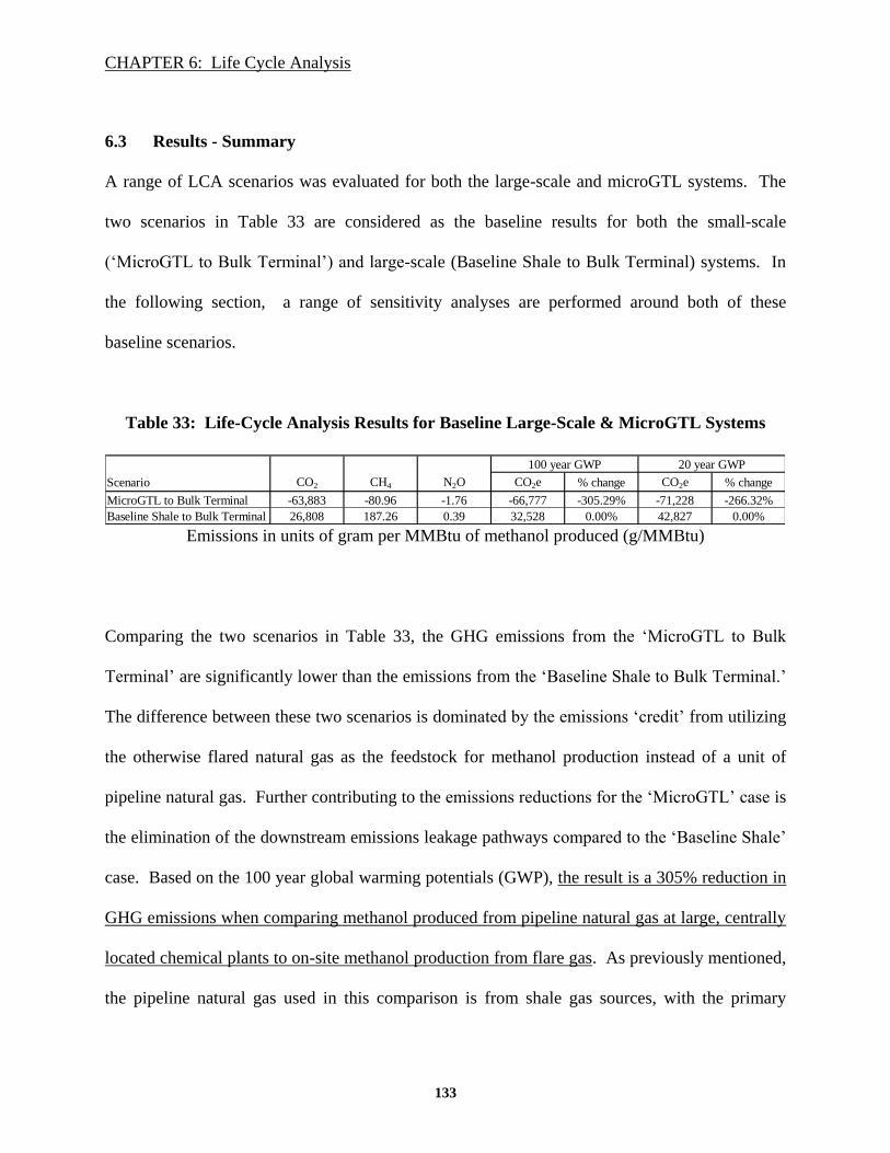
CHAPTER 6: Life Cycle Analysis
133
6.3 Results - Summary
A range of LCA scenarios was evaluated for both the large-scale and microGTL systems. The
two scenarios in Table 33 are considered as the baseline results for both the small-scale
(‘MicroGTL to Bulk Terminal’) and large-scale (Baseline Shale to Bulk Terminal) systems. In
the following section, a range of sensitivity analyses are performed around both of these
baseline scenarios.
Table 33: Life-Cycle Analysis Results for Baseline Large-Scale & MicroGTL Systems
Emissions in units of gram per MMBtu of methanol produced (g/MMBtu)
Comparing the two scenarios in Table 33, the GHG emissions from the ‘MicroGTL to Bulk
Terminal’ are significantly lower than the emissions from the ‘Baseline Shale to Bulk Terminal.’
The difference between these two scenarios is dominated by the emissions ‘credit’ from utilizing
the otherwise flared natural gas as the feedstock for methanol production instead of a unit of
pipeline natural gas. Further contributing to the emissions reductions for the ‘MicroGTL’ case is
the elimination of the downstream emissions leakage pathways compared to the ‘Baseline Shale’
case. Based on the 100 year global warming potentials (GWP), the result is a 305% reduction in
GHG emissions when comparing methanol produced from pipeline natural gas at large, centrally
located chemical plants to on-site methanol production from flare gas. As previously mentioned,
the pipeline natural gas used in this comparison is from shale gas sources, with the primary
100 year GWP 20 year GWP
Scenario CO2 CH4 N2O CO2e % change CO2e % change
MicroGTL to Bulk Terminal -63,883 -80.96 -1.76 -66,777 -305.29% -71,228 -266.32%
Baseline Shale to Bulk Terminal 26,808 187.26 0.39 32,528 0.00% 42,827 0.00%

CHAPTER 6: Life Cycle Analysis
134
difference between shale and conventional natural gas sources due to the higher GHG emissions
during extraction at the wellhead for shale formations. The emissions reduction potential for the
microGTL case is even greater when considering higher natural gas system methane leakage
cases that will be reviewed in section 6.4.1.
It is important to note that while there is a significant difference in emissions between these two
scenarios, it doesn’t necessarily imply that the microGTL system is an ideal abatement solution
for methane. The methane leakage in the current natural gas system, whether at the wellhead in
the form of flare gas, or downstream in the transmission, distribution, and storage infrastructure,
plays a role in reducing the effectiveness of natural gas as a climate change solution. The
methane leakage in the natural gas system will be reviewed in the sensitivity analysis.
6.3.1 A Note on Global Warming Potentials
For this LCA, the most recent values for Global Warming Potentials (GWPs) reported by the
Intergovernmental Panel on Climate Change (IPCC) were used. The IPCC defines the GWP as
“the time-integrated radiative forcing (RF) due to a pulse emission of a given component,
relative to a pulse emission of an equal mass of CO2” (IPCC et al., 2013). The GWP method is
used to compare a range of greenhouse gases to CO2 on an equivalent basis, and results in a
single CO2-equivalent (CO2e) value. Due to the fact that the GWP calculation is based on a
defined time interval, the CO2e result in this analysis is reported for both 100 year and 20 year
time scales.

CHAPTER 6: Life Cycle Analysis
135
In chapter 8 of the IPCC Working Group I (WGI) Fifth Assessment Report (AR5), the GWP for
CH4 (compared to CO2) is 84 and 28 for the 20 year and 100 year GWP, respectively. In other
words, CH4 has 84 times the radiative forcing of CO2 over a 20 year time span, and 28 times the
radiative forcing of CO2 over a 100 year time span. The GWP method contains a measure of
uncertainty, and has been updated during each of the IPCC assessment reports. Recognizing this
uncertainty, the GWP method is still the most widely used metric to compare emissions for life-
cycle analyses, and these values are used in this study. The 100 year GWP value is the most
commonly used metric, but the 20 year GWP value is also reported here to highlight the short-
term radiative forcing impact that CH4 emissions may have on global warming. The decision
about which GWP value to use (100 year vs. 20 year) is context dependent, and is not explored
in greater detail in this study.
6.4 Results – Sensitivity Studies
6.4.1 Methane Leakage Rates
A range of methane leakage for the natural gas system was evaluated for the large-scale system.
The results from this analysis can then be used as a comparison to the microGTL system that, by
definition in this analysis, contains no methane leakage from extraction or
T&D. Inputs for seven pathways for methane leakage are included in the GREET model and are
listed in Table 32 under the ‘CH4 leakage rate’ parameters. Within these parameters, only
‘Recovery – Completion CH4 Venting’ and ‘Recovery – Workover CH4 Venting’ are different
(higher) for shale sources over conventional sources; the remaining parameters are the same
between shale and conventional sources in GREET. The sum of all of the methane leakage
CHAPTER 6: Life Cycle Analysis
136
parameters results in the ‘CH4 leakage rate: total’ percentage in Table 32. This ‘total’ is a
calculated volume percentage of methane leakage over the total natural gas throughput based on
the seven methane leakage pathways. The baseline case uses the most recent EPA estimate for
methane leakage in the natural gas system, which is approximately 1.2% of system throughput.
Recognizing the wide range methane leakage rate estimates in current literature and on-going
field studies, a range of leakage rates was studied. The methane leakage sensitivity range used
for this analysis is from 0% to 7.26% total methane leakage as a function of natural gas
throughput. The individual methane leakage parameters in GREET (Table 32) were each
adjusted to arrive at the total methane leakage percentage. A more detailed discussion of
methane leakage in the natural gas system is included in section 1.2.2.
Table 34 shows the results for the methane leakage sensitivity analysis. Using the 100 year
GWP, the sensitivity to methane leakage is approximately 3,200 gram of CO2e per 1% of
methane leakage (11,000 g CO2e per 1% for the 20 year GWP). Reducing the methane leakage
from the current EPA estimate (1.2%) to 0% results in a 12% reduction in overall GHG
emissions based on the 100 yr GWP (~32% reduction using the 20 yr GWP). These results are
for large-scale methanol production, and the range of emissions results presented here are for
direct comparison to the small-scale, on-site case.
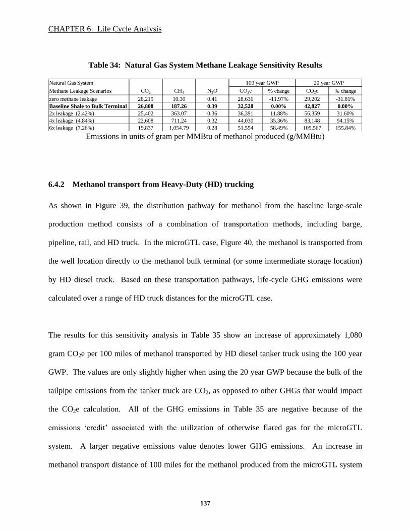
CHAPTER 6: Life Cycle Analysis
137
Table 34: Natural Gas System Methane Leakage Sensitivity Results
Emissions in units of gram per MMBtu of methanol produced (g/MMBtu)
6.4.2 Methanol transport from Heavy-Duty (HD) trucking
As shown in Figure 39, the distribution pathway for methanol from the baseline large-scale
production method consists of a combination of transportation methods, including barge,
pipeline, rail, and HD truck. In the microGTL case, Figure 40, the methanol is transported from
the well location directly to the methanol bulk terminal (or some intermediate storage location)
by HD diesel truck. Based on these transportation pathways, life-cycle GHG emissions were
calculated over a range of HD truck distances for the microGTL case.
The results for this sensitivity analysis in Table 35 show an increase of approximately 1,080
gram CO2e per 100 miles of methanol transported by HD diesel tanker truck using the 100 year
GWP. The values are only slightly higher when using the 20 year GWP because the bulk of the
tailpipe emissions from the tanker truck are CO2, as opposed to other GHGs that would impact
the CO2e calculation. All of the GHG emissions in Table 35 are negative because of the
emissions ‘credit’ associated with the utilization of otherwise flared gas for the microGTL
system. A larger negative emissions value denotes lower GHG emissions. An increase in
methanol transport distance of 100 miles for the methanol produced from the microGTL system
Natural Gas System 100 year GWP 20 year GWP
Methane Leakage Scenarios CO2 CH4 N2O CO2e % change CO2e % change
zero methane leakage 28,219 10.30 0.41 28,636 -11.97% 29,202 -31.81%
Baseline Shale to Bulk Terminal 26,808 187.26 0.39 32,528 0.00% 42,827 0.00%
2x leakage (2.42%) 25,402 363.07 0.36 36,391 11.88% 56,359 31.60%
4x leakage (4.84%) 22,608 711.24 0.32 44,030 35.36% 83,148 94.15%
6x leakage (7.26%) 19,837 1,054.79 0.28 51,554 58.49% 109,567 155.84%

CHAPTER 6: Life Cycle Analysis
138
would result in an increase in emissions (a reduction in the emissions ‘credit’) of ~1.6%, but
would still maintain an emissions advantage of over 300% compared to the baseline large-scale
case.
This emissions result from GREET assumes that the tanker truck makes a roundtrip, returning to
the location of the methanol production with an empty tank. This assumption may be
conservative, and actual GHG emissions from HD trucking could be lower than reported in this
analysis if an optimized tanker truck routing scheme is implemented to minimize the distance
that the tanker truck is required to drive with an empty tank.
Table 35: Results from HD trucking distance sensitivity study
Emissions in units of gram per MMBtu of methanol produced (g/MMBtu)
6.4.3 Small-Scale GTL Conversion Efficiency
It is likely that this microGTL system will have lower overall system conversion efficiency (from
methane to methanol) than a large-scale methanol production facility. Recognizing this
uncertainty, the economic sensitivity to conversion rate was reviewed in section 4.4.5, and the
emissions sensitivity is included here. A range of conversion efficiency around a baseline value
(-15% to +10%) was considered. Table 36 summarizes the results of this sensitivity study.
These results show that the CO2e values are fairly insensitive to changes in conversion
HD Trucking Sensitivity 100 year GWP 20 year GWP
CO2 CH4 N2O CO2e % change CO2e % change
MicroGTL, 0mi -66,449 -69.98 -1.50 -68,947 1.27% -72,794 1.29%
MicroGTL, truck 80mi -65,623 -68.80 -1.49 -68,082 0.00% -71,865 0.00%
MicroGTL, truck 200mi -64,385 -67.02 -1.47 -66,786 -1.90% -70,471 -1.94%
MicroGTL, truck 400mi -62,321 -64.06 -1.44 -64,625 -5.08% -68,147 -5.17%
MicroGTL, truck 600mi -60,258 -61.10 -1.41 -62,465 -8.25% -65,824 -8.41%

CHAPTER 6: Life Cycle Analysis
139
efficiency. The reason for this is that as the conversion efficiency is reduced, more methane is
required to produce a fixed unit of methanol. During this process, more methane is converted to
CO2, increasing the ‘flare’ characteristic of this system. From an economic perspective, using
more methane to produce the same quantity of methanol may not be desirable, but from the
perspective of GHG emissions, changes to the conversion efficiency do not appear to
significantly impact the LCA results. Taking this a step further, under a scenario with a high
penalty for violating a flaring regulation combined with a depressed market for methanol, there
could be a case for reducing the conversion efficiency.
Based on the results of this particular sensitivity study, the scenario with a 10% reduction in
conversion efficiency was used as the baseline case for the MicroGTL system in Table 33,
section 6.3 (in bold in Table 36). A reduced conversion result was used for the baseline for the
MicroGTL system in an attempt to consider the likely reduction in conversion efficiency over
large-scale systems.44
Table 36: Results from Conversion Efficiency Sensitivity Study
Emissions in units of gram per MMBtu of methanol produced (g/MMBtu)
44 The large-scale system baseline was based on the default input in GREET, and referenced in Table 33.
Conversion Efficiency Sensitivity 100 year GWP 20 year GWP
CO2 CH4 N2O CO2e % change CO2e % change
MicroGTL, -15% eff -62,746 -88.894 -1.933 -65,925 -3.17% -70,812 -1.47%
MicroGTL, -10% eff -63,883 -80.955 -1.758 -66,777 -1.92% -71,228 -0.89%
MicroGTL, -5% eff -64,827 -74.362 -1.613 -67,485 -0.88% -71,573 -0.41%
MicroGTL -65,623 -68.799 -1.491 -68,082 0.00% -71,865 0.00%
MicroGTL, +5% eff -66,305 -64.043 -1.386 -68,593 0.75% -72,114 0.35%
MicroGTL, +10% eff -66,894 -59.929 -1.296 -69,035 1.40% -72,330 0.65%

CHAPTER 6: Life Cycle Analysis
140
6.4.4 Engine reformer replacement
The inexpensive engine reformer system is a key driver to support the economic viability of this
microGTL system. In the current economic system model, the engine is replaced every two
years (refer to the system specifications in Table 14 in section 4.4). From an economic
perspective, the frequent replacement of the engine reformer does not negatively impact the
overall economics of the system. However, from a GHG emissions perspective the impact of the
engine reformer replacement should be evaluated. The first step in the LCA for the engine
reformer system is to estimate the GHG emissions attributable to the manufacturing of the
engine. For this analysis, the GREET vehicle-cycle model was used to provide the
manufacturing emissions for the engine (A Burnham, Wang, & Wu, 2006). The GREET
vehicle-cycle model examines the energy and emissions from vehicle production and disposal,
and can provide this information by vehicle sub-section. For this analysis, the emissions from
the ‘Powertrain System’ were used to estimate the engine reformer emissions. The latest version
of the GREET vehicle-cycle model (2015) contains vehicle manufacturing emissions for a large,
light-duty pick-up truck with a 5.3L V-8 engine (Kelly, Burnham, Sullivan, Elgowainy, & Wang,
2015). The emissions attributed to this engine were used for this analysis and scaled to the
engine displacement for the commercial scale engine reformer system. The engine
manufacturing emissions are summarized in Table 37.
Table 37: Engine Manufacturing Emissions
Powertrain system 100 year GWP 20 year GWP
gram per lifetime CO2 CH4 N2O CO2e CO2e
5.3 Liter from GREET 1,007,585 2,718 25.98 1,118,111 1,267,586
49 Liter Engine Reformer 9,315,408 25,130 240.16 10,337,253 11,719,191
CHAPTER 6: Life Cycle Analysis
141
The next step is to consider the engine manufacturing emissions as part of the overall microGTL
system in terms of emissions per MMBtu of methanol produced. First, the MMBtu of methanol
per engine reformer system must be calculated. At 80% time-on-stream and a 2 year lifetime for
the engine reformer system, the MMBtu/engine is:
57,250 btu/gal x 42 gal/bbl x 49 bbl/day x 0.80 x 365 d/yr x 2 yr = 68,807 MMBtu/engine (24)
Using this result and the emissions from Table 37, the emissions from engine manufacturing per
MMBtu of methanol produced can be calculated (for 100 year GWP):
10,337,253 g CO2e / 68,807 MMBtu = 150 g CO2e / MMBtu (25)
This result offsets the baseline life-cycle emissions for the microGTL system from Table 33.
The emissions due to engine manufacturing, 150 g CO2e/MMBtu of methanol produced, are
small by comparison to the overall life-cycle emissions ‘credit’ for the microGTL plant, -66,777
g CO2e/MMBtu of methanol produced (~0.22%). As might be expected, the in-use emissions
dominate the system life-cycle emissions.

CHAPTER 7: Discussion and Future Work
142
CHAPTER 7: Discussion and Future Work
Recent advances in oil and gas extraction technologies have expanded the resource base for
natural gas. These new resources are often in the form of short lifetime, spatially distributed oil
and gas wells. With this resource expansion, there has been an overall increase in natural gas
flaring from oil and gas well sites. The extent of natural gas flaring has created an opportunity to
utilize this otherwise wasted resource to convert it to a useful product, while reducing the
environmental hazard of flaring GHGs into the atmosphere. The distributed nature of this new
resource has motivated development of small-scale GTL systems aimed at monetizing this
‘stranded’ asset. This thesis delivers a techno-economic and environmental analysis of one such
small-scale GTL system to produce methanol using a developed, mass-manufactured internal
combustion engine as a reformer for natural gas to syngas. While this particular technology is
aimed at methanol production, the engine reformer may have broad reaching applications in
areas where syngas is needed but difficult to produce at small scales.
This thesis builds on earlier work by the Lenfest Center for Sustainable Energy. Dahlgren’s
thesis concluded that “small unit scale should be included and properly evaluated in future
technology development” and his work specifically highlighted liquid fuels synthesis using
stranded natural gas as a feedstock as a technology suited for small-unit scale (Dahlgren, 2014).

CHAPTER 7: Discussion and Future Work
143
This thesis advances the findings from Dahlgren, and demonstrates an applied technology
example of a microGTL system. Based on the current status of this system, as it traverses down
the learning curve it may eventually compete against historically large methanol production
units.
The economic analysis presented in this thesis compares the methanol production cost for this
microGTL system against large methanol plants. The results of this analysis show that in order
for the microGTL plant to compete with large unit production, the microGTL plant capital cost
will need to be reduced, and the natural gas feedstock must be received at a discount. It is
reasonable to expect that the natural gas feedstock will indeed be available at a discount over
industrial pipeline quality natural gas, as this microGTL system is designed to utilize otherwise
flared natural gas at the well site. The plant capital cost is dominated by the compressor system,
suggesting that future work should focus on developing small-scale syngas compressor
technologies to support technologies such as the microGTL system reviewed in this thesis.
Taking this a step further, it is possible that the economics of using mass-produced internal
combustion engines could be expanded to other technologies that have historically relied on
large units of operation, including compressors for syngas.
The economic analysis also compares the intermediate syngas production step for the microGTL
system against syngas production from large petrochemical plants. The results of this analysis
suggests that the current syngas production cost for the microGTL system may already be
competitive with large-scale syngas production, driven by the low cost of the engine reformer
system. While this result is preliminary, it contributes to the dialogue on the potential for
CHAPTER 7: Discussion and Future Work
144
existing mass-manufactured systems, in this case internal combustion engines, to enable new
technologies at significantly smaller scales compared to historical norms in the energy and
chemical processing industries.
Expanding the development of small-scale, distributed conversion technologies will likely
contribute to enabling new technologies. A new demand for small-scale air separation and
compressor technologies may develop to support the expanded commercialization of small-scale
GTL systems. If small-scale, economic air separation technologies become deployable in the
future, the impact on this microGTL system and other similar systems where compression costs
dominate capital cost may be significant. Specifically as it pertains to this microGTL system, a
95% O2 configuration would reduce the overall compression requirement to the point that the
engine reformer system may be able to supply most or all of the compression necessary for the
methanol reactor, thus eliminating the need for an external compressor system and providing
potentially significant reductions to the system capital cost.
Balance of plant components pertaining to sensor technology, controls systems, and remote data
analysis will also play key roles towards the path to broad commercialization of this technology.
The ability to remotely monitor individual component and overall system performance will
contribute to reduced labor cost and process optimization. While not specifically reviewed in
this economic analysis, it is expected that this system will take advantage of the rapidly
developing state of the art in the field of remote monitoring and controls systems in support of
distributed energy systems. Future work should focus specifically on advancing the state of the

CHAPTER 7: Discussion and Future Work
145
art to support small-scale conversion technologies such as the microGTL system presented in
this thesis.
Future work should build on the economic analysis in this thesis to include additional economic
drivers unique to small-scale GTL systems. Determining an economic value for the modular,
distributed design of systems such as this to address distributed resources is one such example.
Dahlgren’s work identified the advantage of quicker ‘learning’ inherent to small, short-lived
systems over large scale units, and also identified the increased value from the “option to wait.”
It is the “option to wait” that is particularly applicable to this microGTL system and to
distributed natural gas in general, and should be explored further as it pertains to this technology
and the fossil fuel extraction industry.
The recent, significant decreases in both domestic natural gas and global oil prices highlight an
economic advantage that distributed, short-lived technologies may have over large units designed
to operate for decades. A small, distributed, short-lived system can base its deployment strategy
on short-term market drivers, exploiting the volatility that has permeated the global fossil fuel
industry due to the global expansion of fracking technology, and reducing the risk associated
with long-term capital investments under the increased, sustained volatility. The dynamics of
economic drivers such as these should be incorporated into future work on this subject.
The commercialization and broad implementation of technologies such as the microGTL system
evaluated in this thesis will contribute to the growth of distributed energy infrastructures. From
an environmental perspective, deploying distributed, short-lived units will reduce or eliminate

CHAPTER 7: Discussion and Future Work
146
the relative permanence of large-scale units, and support more rapid transitions away from fossil-
based energy sources. While addressing associated gas from shale oil and gas extraction is a
likely early application of this new technology, it is also possible that new business models
aimed at converting small, remote, sources of methane could be defined, such as biogas from
agricultural and municipal waste. Waste water treatment facilities that utilize methanol in a
denitrification process may be ideally suited as early adopters of this microGTL system.
The life-cycle analysis in this thesis quantifies the net GHG emissions for the microGTL system
from utilizing otherwise flared natural gas to produce methanol. The result highlights the impact
that using a waste stream may have on reducing GHG emissions from a growing fossil fuel
extraction process. While more detailed analysis aimed at specific market cases is necessary,
this LCA result supports the potential for systems such as this to provide an economic solution to
addressing an environmental problem.
Technologies such as this may encourage an expanded use of methanol into the transportation
sector. While the well-to-pump emissions for methanol are less than for gasoline and diesel, and
thus a net reduction in GHG emissions compared to those fuels, the end result would still be the
emission of fossil carbon into the atmosphere. A potentially significant environmental benefit of
expanding methanol into the transport sector could however be a transition away from fossil-
based methanol towards sustainable methanol, as promoted by George Olah in his book, “The
Methanol Economy,” and in more recent publications on the topic (Olah, Goeppert, & Prakash,
2009; Olah, 2013). An important first step towards sustainable methanol will be the expansion

CHAPTER 7: Discussion and Future Work
147
of a methanol infrastructure, supported by small, distributed, short-lived systems such as the
microGTL technology evaluated in this thesis.
In the short-term, a hurdle that exists for this technology is the transition from development and
proof-of-concept to commercialization. Beyond demonstrating the technical feasibility of this
system, a robust economic case must be made to support enough capital investment into this new
field to drive commercialization. Volatility and uncertainty in medium- and long-term oil and
gas markets may create resistance to new investment. Domestic policy drivers aimed at flaring
reduction and downstream methane leakage will impact the relative importance of technologies
like this microGTL system. Changing dynamics in natural gas as an internationally traded fossil
fuel may also present new challenges.

Bibliography
148
Bibliography
ADI Analytics LLC. (2015). Natural Gas Utilization via Small-Scale Methanol Technologies.
Allen, D. T., Torres, V. M., Thomas, J., Sullivan, D. W., Harrison, M., Hendler, A., … Seinfeld,
J. H. (2013). Measurements of methane emissions at natural gas production sites in the
United States, 110(44). doi:10.1073/pnas.1304880110/-
/DCSupplemental.www.pnas.org/cgi/doi/10.1073/pnas.1304880110
Arrhenius, S. (1896). On the Influence of Carbonic Acid in the air upon the Temperature of the
Ground. Philosophical Magazine and Journal of Science, (April 1896), 237–276.
Brandt, A., Heath, G., Kort, E., O’Sullivan, F., Petron, G., Jordaan, M., … Stucky, G. (2014).
Methane Leaks from North American Natural Gas Systems. Science, 343(6172), 733–735.
doi:10.1126/science.1247045
Bromberg, L., Green, W. H., Sappok, A., Cohn, D. R., & Jalan, A. (2014). Engine Reformer
Systems for Lower Cost, Smaller Scale Manufacturing of Liquid Fuels.
Burnham, A., Han, J., Clark, C. E., Wang, M., Dunn, J. B., & Palou-Rivera, I. (2012). Life-cycle
greenhouse gas emissions of shale gas, natural gas, coal, and petroleum. Environmental
Science & Technology, 46(2), 619–27. doi:10.1021/es201942m
Burnham, A., Wang, M., & Wu, Y. (2006). Development and Applications of GREET 2.7 — The
Transportation Vehicle-Cycle Model. doi:10.2172/898530
Camuzeaux, J. R., Alvarez, R. A., Brooks, S. A., Browne, J. B., & Sterner, T. (2015). Influence
of Methane Emissions and Vehicle Efficiency on the Climate Implications of Heavy-Duty
Natural Gas Trucks. Environmental Science & Technology, 49(11), 6402–6410.
doi:10.1021/acs.est.5b00412
Choi, G. N., Kramer, S. J., Tam, S. S., & Fox, J. M. (1997). Design and economics of a Fischer-
Tropsch plant for converting natural gas to liquid transportation fuels. ACS Division of Fuel
Chemistry, Preprints, 42(2), 667–670. doi:10.1016/S0140-6701(97)84578-X
Cuenca, R. M., Gaines, L. L., & Vyas, a D. (1999). Evaluation of Electric Vehicle Production
and Operating Costs. Center for Transportation Research, Energy Systems Division,
Argonne National Laboratory.
Dahlgren, E. (2014). Rescaling Capital: The Potential of Small-Scale and Mass-Produced
Physical Capital in the Energy and Materials Processing Industries. Columbia University.
Retrieved from http://academiccommons.columbia.edu/catalog/ac:166812
Dahlgren, E., Göçmen, C., Lackner, K., & van Ryzin, G. (2013). Small Modular Infrastructure.
The Engineering Economist, 58(4), 231–264. doi:10.1080/0013791X.2013.825038
Fleisch, T. (2014). Associated Gas Monetization via miniGTL Conversion of flared gas into
liquid fuels & chemicals - Update January 2014. World Bank/Global Gas Flare Reduction
Partnership.

Bibliography
149
Fleisch, T. (2015). Associated Gas Monetization via miniGTL Conversion of flared gas into
liquid fuels & chemicals 2015 : GTL is a commercial reality for flaring reduction Report III,
(July), 1–19.
Fleisch, T., & Sills, R. (2014). DME Fundamentals. In 6th International DME Conference.
Gupta, R. (Research T. I. (2015). Conversation with Raghubir Gupta.
Howarth, R. W., Santoro, R., & Ingraffea, A. (2011). Methane and the greenhouse-gas footprint
of natural gas from shale formations. Climatic Change, 106(4), 679–690.
doi:10.1007/s10584-011-0061-5
Index Mundi. (2015). Retrieved from http://www.indexmundi.com/commodities/
International Organization of Motor Vehicle Manufacturers. (2015). Retrieved from
http://www.oica.net/category/production-statistics/2013-statistics/
IPCC, Stocker, T., Qin, D., Plattner, G.-, Tignor, M., Allen, S., … Midgley, P. (2013). The
Physical Science Basis. Contribution of Working Group I to the Fifth Assessment Report of
the Intergovernmental Panel on Climate Change. Retrieved from
http://www.ipcc.ch/report/ar5/wg1/
Karim, G., & Wierzba, I. (2008). The production of hydrogen through the uncatalyzed partial
oxidation of methane in an internal combustion engine. International Journal of Hydrogen
Energy, 33(8), 2105–2110. doi:10.1016/j.ijhydene.2008.01.051
Karim, G., & Zhou, G. (1993). A kinetic investigation of the partial oxidation of methane for the
production of hydrogen. International Journal of Hydrogen Energy, 18(2), 125–129.
doi:10.1016/0360-3199(93)90198-J
Karion, A., Sweeney, C., Pétron, G., Frost, G., Michael Hardesty, R., Kofler, J., … Conley, S.
(2013). Methane emissions estimate from airborne measurements over a western United
States natural gas field. Geophysical Research Letters, 40(16), 4393–4397.
doi:10.1002/grl.50811
Kelly, J., Burnham, A., Sullivan, J., Elgowainy, A., & Wang, M. (2015). Addition of New
Conventional and Lightweight Vehicle Models in the GREET Model.
Kolwich, G. (2012). Light-Duty Vehicle Technology Cost Analysis – European Vehicle Market
(Phase 1).
Kringstad, J. J. (2013). North Dakota Natural Gas - A Detailed Look at Natural Gas Gathering.
North Dakota Pipeline Authority. Retrieved from www.northdakotapipelines.com
Lakshminarayanan, P. A., & Kanase, K. (2013). A Basis for Estimating Mechanical Efficiency
and Life of a Diesel Engine from its Size , Load Factor and Piston Speed. Society of
Automotive Engineers, International. doi:10.4271/2011-01-2211
Lim, E. G., & Cheng, W. K. (2015). The Engine Reformer : Syngas Production in Engines Using
Spark- Ignition and Metallic Foam Catalysts. Massachusetts institute of Technology.
Retrieved from http://dspace.mit.edu/

Bibliography
150
Lutz, M. (2013). A Bakken Producer’s Regional View on Gas & NGL Markets. Retrieved from
http://www.platts.com/IM.Platts.Content/ProductsServices/ConferenceandEvents/2013/pc3
18/presentations/Michael_Lutz.pdf
Moore, C. W., Zielinska, B., Pétron, G., Jackson, R. B., Pe, G., & Jackson, R. B. (2014). Air
Impacts of Increased Natural Gas Acquisition, Processing, and Use: A Critical Review.
Environmental Science & Technology, 48, 8349–8359. doi:10.1021/es4053472
Morsy, M. H. (2014). Modeling study on the production of hydrogen/syngas via partial oxidation
using a homogeneous charge compression ignition engine fueled with natural gas.
International Journal of Hydrogen Energy, 39(2), 1096–1104.
doi:10.1016/j.ijhydene.2013.10.160
Myhre, G., Shindell, D., Bréon, F.-M., Collins, W., Fuglestvedt, J., Huang, J., … Zhan, H.
(2013). 2013: Anthropogenic and Natural Radiative Forcing. Climate Change 2013: The
Physical Science Basis. Contribution of Working Group I to the Fifth Assessment Report of
the Intergovernmental Panel on Climate Change. doi:10.1017/ CBO9781107415324.018
National Academy of Sciences. (2009). Liquid Transportation Fuels from Coal and Biomass:
Technological Status, Costs, and Environmental Impacts. Energy. doi:ISBN-10: 0-309-
13712-8
National Energy Technology Laboratory. (2013). Analysis of Natural Gas-to Liquid
Transportation Fuels via Fischer-Tropsch. National Energy Technology Laboratory, U.S.
Department of Energy, Office of Fossil Energy.
Noureldin, M. M. B., Elbashir, N. O., & El-Halwagi, M. M. (2014). Optimization and selection
of reforming approaches for syngas generation from natural/shale gas. Industrial and
Engineering Chemistry Research, 53(5), 1841–1855. doi:10.1021/ie402382w
Olah, G. a. (2013). Towards oil independence through renewable methanol chemistry.
Angewandte Chemie (International Ed. in English), 52(1), 104–7.
doi:10.1002/anie.201204995
Olah, G. a, Goeppert, A., & Prakash, G. K. S. (2009). Chemical recycling of carbon dioxide to
methanol and dimethyl ether: from greenhouse gas to renewable, environmentally carbon
neutral fuels and synthetic hydrocarbons. The Journal of Organic Chemistry, 74(2), 487–98.
doi:10.1021/jo801260f
Pederstad, A., Gallardo, M., & Saunier, S. (2015). Improving utilization of associated gas in US
tight oil fields.
Pei, P., Korom, S. F., Ling, K., & Nasah, J. (2014). Cost comparison of syngas production from
natural gas conversion and underground coal gasification. Mitigation and Adaptation
Strategies for Global Change. doi:10.1007/s11027-014-9588-x
Peischl, J., Ryerson, T. B., Aikin, K. C., Gouw, J. A., Gilman, J. B., Holloway, J. S., … Parrish,
D. D. (2015). Journal of Geophysical Research : Atmospheres Quantifying atmospheric
methane emissions from the. doi:10.1002/2014JD022697.Received
Pétron, G., Karion, A., Sweeney, C., Miller, B. R., Montzka, S. A., Frost, G. J., … Schnell, R.

Bibliography
151
(2014). A new look at methane and nonmethane hydrocarbon emissions from oil and natural
gas operations in the Colorado Denver-Julesburg Basin. Journal of Geophysical Research :
Atmospheres, 1–17. doi:10.1002/2013JD021272.Received
Rubin, E. S., Chen, C., & Rao, A. B. (2007). Cost and performance of fossil fuel power plants
with CO2 capture and storage. Energy Policy, 35(9), 4444–4454.
doi:10.1016/j.enpol.2007.03.009
Schwietzke, S., Griffin, W. M., Matthews, H. S., & Bruhwiler, L. M. P. (2014). Global natural
gas fugitive emissions rates based on atmospheric methane and ethane constraints. In
preparation.
U.S. EIA. (2012). Petroleum Market Module - Assumptions to the Annual Energy Outlook.
Retrieved from http://www.eia.gov/forecasts/aeo/assumptions/pdf/petroleum.pdf
U.S. Energy Information Administration. (2014). Annual Energy Outlook 2014.
U.S. Energy Information Administration. (2015). Drilling Productivity Report - for key tight oil
and shale gas regions.
U.S. Energy Information Administration. (2016). Carbon dioxide emissions per kilowatthour.
Retrieved from https://www.eia.gov/tools/faqs/faq.cfm?id=74&t=11
U.S. Environmental Protection Agency. (2015). Inventory of U.S. Greenhouse Gas Emissions
and Sinks: 1990 - 2013, 1–564. Retrieved from
http://www.epa.gov/climatechange/Downloads/ghgemissions/US-GHG-Inventory-2015-
Main-Text.pdf
United States Bureau of Labor Statistics. (2015). Producer Price Index by Commodity for
Intermediate Demand By Commodity Type: Processed Fuels and Lubricants for
Intermediate Demand [WPUID613]. Retrieved from
https://research.stlouisfed.org/fred2/series/WPUID613/
United States Environmental Protection Agency. (2012). Light-Duty Vehicle Mass Reduction
and Cost Analysis — Midsize Crossover Utility Vehicle Light, 878. Retrieved from
http://www.epa.gov/otaq/climate/documents/420r12026.pdf
Vyas, A., Santini, D., & Cuenca, R. (2000). Comparison of Indirect Cost Multipliers for vehicle
manufacturing.
Wang, M., Wu, Y., & Elgowainy, A. (2007). Operating Manual for GREET: Version 1.7.
Wigley, T. M. L. (2011). Coal to gas: the influence of methane leakage. Climatic Change,
108(3), 601–608. doi:10.1007/s10584-011-0217-3
Wocken, C. A., Stevens, B. G., Almlie, J. C., & Schlasner, S. M. (2013). End-Use Technology
Study – An Assessment of Alternative Uses for Associated Gas. Retrieved from
http://www.undeerc.org/bakken/pdfs/CW_Tech_Study_April-2013.pdf
Wood, D. a., Nwaoha, C., & Towler, B. F. (2012). Gas-to-liquids (GTL): A review of an
industry offering several routes for monetizing natural gas. Journal of Natural Gas Science
and Engineering, 9, 196–208. doi:10.1016/j.jngse.2012.07.001

Bibliography
152
Yamamoto, T., Kaneko, K., Kuwae, K., & Hiratsuka, K. (1963). Production of Synthesis Gas by
an Internal Combustion Engine. World Petroleum Congress.

Appendix A
153
Appendix A
Preliminary Case Study
NOTE: As part of the ARPA-E project that has funded this research, quarterly reports are
submitted to review and summarize the status of the on-going project development. In the most
recent quarter (ending Dec. 2015), an economic case study aimed at taking an initial look at
utilizing flare gas and associated natural gas liquids in the Bakken oil field was performed. The
results of this case study are presented here.
Overview
This case study reviews the economic model results for the microGTL system aimed at flaring
reduction utilizing associated gas from tight oil production in the Bakken oil field. While the
Bakken formation in North Dakota is used for this analysis, the framework developed for this
case study should be applicable to other associated gas sources as well (i.e. the Eagle Ford
formation in Texas). A recent study commissioned by the Clear Air Task Force and carried out
by Carbon Limits AS, “Improving utilization of associated gas in US tight oil fields,” was used
as a reference throughout this case study as a basis for the economic model inputs specifically
pertaining to the Bakken region (Pederstad et al., 2015).

Appendix A
154
The primary method for utilizing associated gas in the Bakken field is through gathering
pipelines. However, the pipelines are not always economical. In cases of short-lived or
geographically remote wells, gathering pipelines are rarely installed, and the associated gas is
instead flared. Even at well locations where gathering pipelines have been installed, flaring may
occur when the quantity of associate gas is greater than the capacity of the pipeline. In other
cases, the peak production for a well occurs before a gathering pipeline has been installed,
resulting in a large quantity of associated gas flared during a short period of time (typically
during the first few months of production).
The Carbon Limits report evaluates several technologies aimed at addressing flaring under these
well conditions, specifically at the Bakken and Eagle Ford tight oil formations. The associated
gas produced from these formations is considered ‘wet,’ containing not only dry components
(mostly methane and in some cases, ethane), but varying quantities of valuable natural gas
liquids (‘NGLs’: propane, butane, pentane, etc.). The recovery of NGLs, while economical
under a range of conditions, does not significantly contribute to flaring reduction (reduction of 5-
20%). This case study evaluates a scenario that combines NGL recovery with methanol
production using the microGTL system. Combining the NGL recovery with methanol
production improves the flaring reduction (> 90% reduction) and provides a potentially more
profitable revenue stream.

Appendix A
155
Background on associated gas characteristics in the Bakken field
In 2013, 32% of associated gas in the Bakken was flared, with 14% from isolated wells and 18%
from wells connected to gathering pipelines. The remaining 68% of the associated gas was
captured and fed into a natural gas pipeline. Combining the Bakken and Eagle Ford formations,
flaring from associated gas production was estimated at 125 Bcf (billion cubic feet) in 2013.
With the goal of evaluating technologies aimed at reducing this significant quantity of flaring of
associated gas, the Carbon Limits report identified factors unique to these tight oil formations
that should be considered when evaluating possible technical solutions. Among these key factors
are:
Decline rates: overall well production (oil & associated gas) declines 50-60% during the
first year.
Total well production: 30% of total well production occurs during the first year, and 50%
by the end of the second year.
High intraday variability: production volumes can vary by 10x throughout a day.
NGLs: the rich (wet) associated gas contains varying, large quantities of these valuable
components that should be monetized.
Therefore, a successful associated gas utilization technology should be scalable over time,
immediately deployable, able to manage variability, and compliment NGL recovery. These
system characteristics align well with the engine reformer microGTL system under development.

Appendix A
156
Business & Economic Model
For this case study, a service provider model has been defined with the microGTL company as
the primary provider. A system diagram summarizing the expenses and revenue streams is
shown in Figure 41. For this system, in addition to paying its own operating expenses, the
microGTL service provider pays for NGL separation services, as well as a price, if any, for the
associated gas. The revenues are generated from the methanol produced from the microGTL
system and the NGLs it obtains from the associated gas through the external NGL separation
service. Another possible business model, to be evaluated in the next quarter, considers the
microGTL system as part of a service fee model where the Exploration and Production (E&P)
company pays a fee for conversion of its natural gas to methanol.
Figure 41: Service Provider Model
The net-present-value (NPV) model previously developed to estimate the methanol production
cost of the microGTL system was used as a basis to calculate the NPV for this service provider
model. For this economic analysis, several industry sources were used to define the input
assumptions for the NGLs used in this modified economic model (Kringstad, 2013; Lutz, 2013;
Wocken, Stevens, Almlie, & Schlasner, 2013). Table 38 summarizes the input variables used for
the economic model, and includes the NPV result. A tax rate of 35% was used, along with a
MicroGTL
SERVICE PROVIDER
IRR, Plant Life, Tax Rate
Expenses
O&M
Plant Refurbishment
NGL Service Fee
NG Cost
Transportation
Revenue
Methanol ($/gal)
C3+ NGLs ($/gal)

Appendix A
157
plant life of 16 years and a cost of capital (discount rate for the NPV calculation) of 17.5%. The
cost of capital is high relative to mature, large-scale petrochemical facilities (5%-10%). This
conservative initial estimate for the cost of capital is used as a way to capture the risk associated
with this new technology and the inherent variability of this resource. Items highlighted in
yellow are baseline assumptions, however a range of values are likely for these particular inputs.
An initial sensitivity study is included in this analysis for a subset of factors, and will be refined
through the next quarter.
Theoretical supply chain scenarios for both methanol and NGLs were defined by RTI for the
service provider model.45
The methanol supply chain assumes that the methanol is supplied to a
small-to-midsized end user in North Dakota, and is transported by tanker truck. For this
methanol supply chain, a transport distance of 180 miles (via heavy duty truck) is defined based
on a scenario with methanol supplied to a small-to-midsized end user in North Dakota. For the
sensitivity study, a baseline of 90 miles is defined so that a +/- of 90 miles can be evaluated
(encompassing zero miles and 180 miles, the supply chain scenario).
For the NGL supply chain, the propane spot price at Mont Belvieu, TX is used for the NGL sell
price. Assuming that this spot price includes the transport cost for propane, the supply chain
includes the transport cost from Williston, ND to Mont Belvieu, TX (1,600 mile). A baseline
distance of 800 miles is used, and is also evaluated in the sensitivity analysis. The methanol
transport cost was estimated using results from a recent National Academy of Sciences text that
estimated ethanol fuel transport cost by mode (National Academy of Sciences (NAS), 2009).
45 Philip Watson, Emerging Energy Technologies Division, RTI. Dec. 2015.

Appendix A
158
The NGL transport cost was taken from a recent study by Hess Corp. that estimated NGL
transport costs (Lutz, 2013).
For the baseline case study scenario, the methanol and NGLs revenue was based on the average
annual spot prices for the years 2010 to 2014 from Methanex and propane at Mont Belvieu, TX,
respectively. This multi-year average was used due to the relative stability in liquid hydrocarbon
prices during this period (Figure 1 in Section 1.2.1). The recent volatility and downward
pressure on both oil and natural gas prices through 2015 changes the economic viability of this
service provider model; two alternate scenarios are reviewed below as well to highlight these
current market conditions. The first alternate scenario uses average annual methanol and
propane prices for 2015, and the second scenario is based on prices from December 2015. A
range of methanol and propane prices are also included in the sensitivity study so that the impact
of these market conditions can be quantified as part of the broader study.
Figure 42 is a plot of per-year NPV over the plant lifetime comparing the microGTL system
(microGTL-only) to the system with additional revenue from NGLs (microGTL + NGL). With
the baseline economic assumptions (Table 38), the microGTL (MeOH-only) system breaks even
during year 16 with a cost of capital of 17.5%. The additional revenue from NGLs in the
associated gas stream results in an overall system breakeven point prior to year 6, and an overall
NPV of ~$800,000 over the plant lifetime. These results do not consider the value of meeting
regulation or the CO2 abatement cost. A sensitivity study including the factors highlighted in
yellow in Table 38 follows in the next section.
Appendix A
159
Table 38: Economic Model Inputs and NPV result
System Specifications Value Units
Associated gas flow 0.333 MMscfd
Raw NGL Content 8 gal NGL / Mscf
Share C3+ NGL 50%
Methanol production 6.0 MT/day
Plant availability 1.0 days/day
Component cost - GTL
Total plant capital cost 1,427,769$ $
Refurbishment GTL
Plant refurb period 2.0 years
Refurb cost 63,900.00$ $
Operating Costs
Operation and maintenance 4.82 $/bbl
Natural gas cost 0.5 $/Mscf
MeOH Transport $0.0166 $/bbl/mile
MeOH Transport 180 mile
C3+ Transport $0.0062 $/bbl/mile
C3+ Transport 1600 mile
Annual operating costs
O&M GTL 85,666$ $
NGL Separation Service Fee 0.35 $/gal NGL
NGL Separation Service Fee 170,163$ $
Natural gas 60,773$ $
Transportation MeOH 52,028$ $
Transportation C3+ 115,508$ $
Revenue
Methanol price 470 $/ton
Methanol price 1.41 $/gal
Methanol production cost 0.45 $/gal
Methanol Annual Revenue 700,902$
NGL price 1.14 $/gal
NGL Annual Revenue 554,245$
Total Annual revenue 1,255,147$ $
Corporate Income Tax Rate 35.00% %
Cost of Capital (discount rate for NPV calc) 17.5% %
Assumed Plant Life 16 years

Appendix A
160
Figure 42: Per-year NPV for the MicroGTL System Lifetime
Preliminary Sensitivity Analysis
The variables and ranges used for the sensitivity study are summarized in Table 39. The median
values differ slightly from the case study scenario reviewed above, but the ranges are inclusive of
the case study. The results for the sensitivity analysis are plotted in the tornado chart in Figure
43. As might be expected, small changes to methanol and NGL market prices have a significant
impact on the overall system NPV. The difference between NGL separation cost (‘C3+ sep’ in
Figure 43) and NGL cost (‘C3+ $/gal’) dictates the revenue (or lack thereof) from the NGLs.
While these factors are known based on market conditions, other factors such as the cost of
capital, price for associated gas, and actual transport distance are unknown at this time, and will
continue to be refined during the development of the commercialization plan.

Appendix A
161
Table 39: Range of Values for Sensitivity Study
Figure 43: Service Provider Model Sensitivity Analysis
Variable High Middle Low
Capital cost $ $2,141,654 $1,427,769 $1,070,827
Cost of Cap % 20.0% 17.5% 15.0%
C3+ $/gal $1.20 $1.00 $0.80
MeOH $/ton $450 $400 $350
C3+ gal/Mscf 12 8 4
NG Price $1.00 $0.50 $0.00
Transport Dist -50% 90 & 800 mi 50%

Appendix A
162
Current Market Conditions
The values in Table 40 are the spot prices for methanol and propane for the case study (2010-
2014) and the two alternate revenue scenarios (2015 and Dec. 2015). Holding all other input
factors constant, the revised case study results for the alternate price scenarios are shown in
Figure 44 and Figure 45. With a 17.5% cost of capital, the results do not present an
economically viable scenario. However, for the first alternative scenario (2015 average prices),
the microGTL+ NGL system breaks even at 6% cost of capital. The microGTL-only system
breaks even at 10%. The larger percent decrease in propane vs. methanol from the 2010-2014 to
2015 periods results in a more economically viable system for methanol production only. For
the December-2015-only alternate scenario, the microGTL-only system breaks even at a 4% cost
of capital, and is not viable when considering NGLs due to the further drop in price during this
period.
Table 40: Methanol and Propane Spot Prices for Different Time Periods
2010-2014 2015 Dec. 2015
Methanol $1.41 $1.22 $1.05
Propane $1.14 $0.46 $0.39

Appendix A
163
Figure 44: Per-year NPV for Alternate Scenario using 2015 Average Prices
Figure 45: Per-year NPV for Alternate Scenario using Dec. 2015 Average Prices

Appendix B
164
Appendix B
Table 41 contained the material properties for the streams included in the Aspen engine reformer
system.
Table 41: Material properties for stream flows included in Aspen Engine Reformer model
Intake_1 Intake_2 3 6-ATDC 7 9 Exhaust_1 Exhaust_2
Molecular Weight 25.43 25.43 25.43 21.94 21.94 21.65 21.65 21.65
Molar Density [kgmole/m3] 0.04 0.04 0.21 0.37 0.22 0.21 0.04 0.04
Mass Density [kg/m3] 0.98 0.98 5.24 8.16 4.75 4.46 0.87 0.87
Act. Volume Flow [m3/h] 2581.40 2581.40 483.68 310.48 533.70 567.83 2922.85 2922.85
Mass Enthalpy [kJ/kg] -59.81 -59.81 771.36 771.36 405.93 405.93 -523.07 -523.07
Mass Entropy [kJ/kg-C] 7.02 7.02 7.21 8.70 8.76 8.90 9.12 9.12
Heat Capacity [kJ/kgmole-C] 34.67 34.67 40.78 42.55 39.98 39.35 36.20 36.20
Mass Heat Capacity [kJ/kg-C] 1.36 1.36 1.60 1.94 1.82 1.82 1.67 1.67
LHV Molar Basis (Std) [kJ/kgmole] 141202.09 141202.09 141202.09 86936.53 86936.53 82318.10 82318.10 82318.10
HHV Molar Basis (Std) [kJ/kgmole] 156454.41 156454.41 156454.41 100945.65 100945.65 96221.42 96221.42 96221.42
HHV Mass Basis (Std) [kJ/kg] 6151.22 6151.22 6151.22 4600.14 4600.14 4445.03 4445.03 4445.03
LHV Mass Basis (Std) [kJ/kg] 5551.56 5551.56 5551.56 3961.74 3961.74 3802.76 3802.76 3802.76
Mass Exergy [kJ/kg] 202.53 202.53 977.97 2544.78 2160.26 2311.07 1316.38 1316.38
Partial Pressure of CO2 [kPa] 0.00 0.00 0.00 109.26 57.63 62.54 8.93 8.93
Cost Based on Flow [Cost/s] 0.00 0.00 0.00 0.00 0.00 0.00 0.00 0.00
Act. Gas Flow [ACT_m3/h] 2581.40 2581.40 483.68 310.48 533.70 567.83 2922.85 2922.85
Avg. Liq. Density [kgmole/m3] 27.49 27.49 27.49 31.17 31.17 31.53 31.53 31.53
Specific Heat [kJ/kgmole-C] 34.67 34.67 40.78 42.55 39.98 39.35 36.20 36.20
Std. Gas Flow [STD_m3/h] 2354.75 2354.75 2354.75 2729.32 2729.32 2766.78 2766.78 2766.78
Std. Ideal Liq. Mass Density [kg/m3] 699.25 699.25 699.25 683.95 683.95 682.45 682.45 682.45
Cp/(Cp - R) 1.32 1.32 1.26 1.24 1.26 1.27 1.30 1.30
Cp/Cv 1.32 1.32 1.26 1.24 1.26 1.27 1.30 1.30
Heat of Vap. [kJ/kgmole] 10128.20 10128.20 8959.47 27781.08 27347.94 28190.72 27051.36 27051.36
Kinematic Viscosity [cSt] 29.23 29.23 9.47 8.65 14.00 15.23 63.02 63.02
Liq. Mass Density (Std. Cond) [kg/m3] 1.08 1.08 1.08 0.93 0.93 0.92 0.92 0.92
Liq. Vol. Flow (Std. Cond) [m3/h] 2352.85 2352.85 2352.85 2724.19 2724.19 2761.28 2761.28 2761.28
Liquid Fraction 0.00 0.00 0.00 0.00 0.00 0.00 0.00 0.00
Molar Volume [m3/kgmole] 25.92 25.92 4.86 2.69 4.62 4.85 24.98 24.98
Mass Heat of Vap. [kJ/kg] 398.20 398.20 352.25 1266.00 1246.26 1302.30 1249.66 1249.66
Phase Fraction [Molar Basis] 1.00 1.00 1.00 1.00 1.00 1.00 1.00 1.00
Thermal Conductivity [W/m-K] 0.06 0.06 0.10 0.18 0.17 0.18 0.14 0.14
Viscosity [cP] 0.03 0.03 0.05 0.07 0.07 0.07 0.05 0.05
Cv (Semi-Ideal) [kJ/kgmole-C] 26.36 26.36 32.47 34.24 31.66 31.04 27.89 27.89
Mass Cv (Semi-Ideal) [kJ/kg-C] 1.04 1.04 1.28 1.56 1.44 1.43 1.29 1.29
Cv [kJ/kgmole-C] 26.34 26.34 32.45 34.27 31.69 31.06 27.89 27.89
Mass Cv [kJ/kg-C] 1.04 1.04 1.28 1.56 1.44 1.43 1.29 1.29
Liq. Vol. Flow - Sum(Std. Cond) [m3/h] 2352.85 2352.85 2352.85 2724.19 2724.19 2761.28 2761.28 2761.28
Viscosity Index 0.96 0.96 -1.71 2.39 4.37 4.98 9.11 9.11