a tear in the iron curtain: the impact of western ... · a tear in the iron curtain: the impact of...

A Tear in the Iron Curtain:The Impact of Western Television on Consumption Behavior

Leonardo Bursztyn and Davide Cantoni∗

August 2014

Abstract

This paper examines the impact of exposure to foreign media on the economic behaviorof agents in a totalitarian regime. We study private consumption choices focusing on formerEast Germany, where differential access to Western television was determined by geographicfeatures. Using data collected after the transition to a market economy, we find no evidence ofa significant impact of previous exposure to Western television on aggregate consumption lev-els. However, exposure to Western broadcasts affects the composition of consumption, biasingchoices in favor of categories of goods with high intensity of pre-reunification advertisement.The effects vanish by 1998.

Keywords: Consumption, Media, Television, Advertising, East Germany, Communism

JEL Classification: D12, E21, Z10

∗Bursztyn: UCLA Anderson School of Management. Email: [email protected]. Cantoni: University of Mu-nich, CEPR, and CESifo. Email: [email protected]. Previous drafts of this paper have been circulated under the title“Clueless? The Impact of Television on Consumption Behavior.” We are grateful to Philippe Aghion, Alberto Alesina,Stefano DellaVigna, Nicola Fuchs-Schundeln, Matthew Gentzkow, Larry Katz, David Laibson, Yona Rubinstein, AndreiShleifer, Nico Voigtlander, Romain Wacziarg, and Noam Yuchtman for helpful comments, as well as seminar audiencesat the EEA Annual Meeting, the NBER summer institute, and at Harvard, Heidelberg, HU Berlin, Linz, LSE, UCLA, UPenn, and UPF. We thank Tobias Hauck and Maximilian W. Muller for excellent research assistance; Hans-R. Guntherfor letting us access the archives of the IM Leipzig; Jeff Blossom for sharing his GIS expertise with us; and Patrick Rothefor professional support with the German income and expenditure survey data. Parts of this research were completedwhile Davide Cantoni was visiting the University of Heidelberg. We appreciate the financial support of the Paul M.Warburg funds.

1 Introduction

In 1980, over 60% of the countries in the world were ruled by autocratic regimes; as of 2010, this

number has decreased to 27%. Still, this number is sizable, and it includes some of the more popu-

lous countries of the world such as China or Iran (Polity IV, 2010).1 In many of these countries, not

only individuals’ choice sets are restricted, but also their information sets, since non-democratic

regimes often limit access to outside sources of information. Indeed, recent history provides sev-

eral episodes of non-democratic regimes restricting access to foreign, independent media, such

as the current censorship of internet content in China (the “Great Firewall”), as well as instances

in which foreign governments attempt to broadcast news and information to countries where the

free flow of information is controlled, such as Radio Free Europe. Although autocratic regimes

generally attempt to seclude their citizens from this information, oftentimes there are cracks in the

walls–physical or digital—erected. Does the information that passes these cracks matter?

We focus on a particularly important element that is often constrained in totalitarian regimes:

individuals’ ability to fulfill their desires of material consumption. Consumption is not only one

of the most fundamental economic decisions but it is also a defining feature of the Western way

of life.2 The destabilizing effects of the desire for higher levels of material consumption have been

observed across a variety of totalitarian regimes and can, of course together with the wish for

personal freedom and civil liberties, be seen as one of causes of the breakdown of the socialist

system.3

This paper considers how former exposure to foreign television during a communist regime

later translated into differences in private consumption. To study this issue, we exploit a natural

experiment: the differential access to West German television broadcasting in East Germany (the

German Democratic Republic, henceforth GDR) during the communist era. Whereas most East

Germans could (and, according to all available evidence, enthusiastically did) watch West Ger-

1Cf. Marshall et al. (2010). Regimes with a Polity IV score of –10 to –6 are classified as “autocratic.”2Adam Smith famously wrote that “[c]onsumption is the sole end and purpose of all production” (Smith 1776, Bk. IV,

ch. 3, pt. 3).3On the role of consumption shortages in East Germany, see Schneider (1996) and Kaminsky (2001). On (Western)

television stoking consumption desire in former Yugoslavia, see Pusnik and Starc (2008). More recently, increasinglevels of consumerism and craving for capitalistic status symbols have been observed in North Korea: Frank (2010),Frank (2012, pp.40–41), Lankov (2013), Economist (2013).

1

man TV channels, the inhabitants of some regions of the GDR were not reached by West German

broadcasts. Those inhabitants, while equally endowed with TV sets, were only able to watch the

East German TV channels, a drab mixture of political propaganda and Soviet-produced movies.

We look at the individuals with access to West German TV broadcasts in former East Germany

as the treatment group of an “experiment” of having been exposed to Western television for over

three decades.

The regions of GDR without access to Western television broadcasts were located either in the

northeastern or in the southeastern corner of the country (see Figures 1 and 3). These regions,

which together made up for approximately one tenth of the East German population, were either

too distant from the Western border or West Berlin, or located in valleys behind mountains that

would block TV broadcasting signals.4 An example is the large and important district of Dresden,

situated in the Elbe valley, which became popularly known as the “valley of the clueless” (Stiehler,

2001).

Empirically analyzing behavior in totalitarian regimes is notoriously difficult due to data lim-

itations. Both official national statistics and survey data are of questionable quality, and revealed

preferences are difficult to observe given the restrictions citizens are subject to. In order to ex-

amine actual consumption behavior, we look at the period immediately following the German

reunification of 1990. Prior to that event, any differences in desired consumption choices between

individuals exposed or not to Western TV could not be reflected by differences in consumption

behavior, as the goods seen on West German TV were not available in communist East Germany.

Consumption in the GDR was strictly regimented by the central planning operated by the Ministry

of Commerce and Provisioning; consumption patterns would be determined by the day-to-day

availability of goods in store. However, after reunification, this obstacle was no longer impeding

the consumption of desired goods by East Germans; any good that had been previously seen on

TV could now, at least in theory, also be purchased in East Germany.5

We assess the impact of long-term Western television exposure on consumption by analyzing

4A confounding factor that could presumably also affect post-reunification consumption patterns in these regionsis their distance from West Germany, which could conceivably have made some Western products less likely to beavailable for purchase. We address this concern in our analysis, by explicitly taking into account distance to the WestGerman border in some regression specifications.

5Moreover, West German broadcasts were available in all regions of former East Germany already in 1990.

2

the first two waves of the German income and expenditure survey (EVS) collected after 1990. We

find important effects of previous exposure to Western television on consumption behavior. The

effects are subtler than a simple change in total consumption or household savings. Indeed, we

find no evidence of significant and quantitatively meaningful effects of West German TV on those

aggregate variables. Our analysis indicates, instead, that Western television affected the composi-

tion of consumption via one of its key elements: advertisements. If changes in the composition of

consumption are to be attributed to West German television, we should expect larger differences

between regions exposed or not to Western television to occur in the consumption of categories

of products with higher intensity of advertisement on West German television.6 We combine the

EVS data with information about the average intensity of advertising of different categories of

goods on the main West German TV channel during the last decade before reunification.

We find that previous exposure to Western television affects the composition of consumption

shortly after reunification, according to the intensity of pre-reunification West German TV ad-

vertisement in different categories of goods: individuals with access to Western television spent

significantly more on goods with high intensity of pre-reunification advertisement. Spending on

a category of goods that had one more minute of advertising per day during the 1980s was 1.5%

higher in parts of East Germany that had the chance to watch these advertisements, relative to the

“untreated” part of East Germany.

We also provide more than just cross-sectional evidence by analyzing also the second post-

Reunification wave of the EVS survey. Our measured effects vanish through time, and are no

longer visible in 1998. Our results are robust to: (i) variations in the definition of the exposure to

treatment, West German television; (ii) restricting the sample to areas surrounding the threshold

for television signal availability (in the spirit of a regression-discontinuity design); (iii) control-

ling for distance to West Germany and its interaction with intensity of advertisement (to rule out

alternative explanations of our findings based on remoteness factors).

Related to our paper by also exploiting the same, sharp change in regime, is the work by

Alesina and Fuchs-Schundeln (2007), which analyzes the impact of several decades of exposure to

6Other factors associated with access to Western television could also potentially affect the composition of consump-tion, such as exposure of goods in TV shows, movies, etc. We focus on the advertisement mechanism.

3

Communism on former East Germans’ preferences for redistribution and state intervention. Our

paper, however, focuses on comparisons within East Germany, as opposed to comparisons be-

tween East and West Germans. Burchardi and Hassan (2011) show that West German regions that

had a large fraction of households with social ties to the East exhibited higher growth in income

per capita in the early years after German reunification. Friehe and Mechtel (2012) provide evi-

dence indicating that after the German Reunification, individuals in former East Germany spent

more resources on visible goods than former West German individuals did. Finally, similarly to

our research design, the paper by Kern and Hainmueller (2009) uses within-East Germany vari-

ation to analyze the effect of exposure to Western media on reported support for the communist

regime, using survey data on stated preferences.

This paper also relates to the recent empirical literature that studies media effects, and particu-

larly the effect of exposure to television. A series of papers look at political outcomes: Enikolopov

et al. (2011) consider independent TV stations and their effect on the 1999 Russian elections;

DellaVigna and Kaplan (2007) report important effects of Fox News on Republican vote shares.

DellaVigna et al. (2011) focus on effects of exposure to radio, and report the unintended effects

of Serbian radio on the likelihood to vote for extreme nationalist parties in Croatia. Gentzkow

(2006) finds a large impact of the expansion of television between 1940 and 1972 on voter turnout.

Gentzkow and Shapiro (2004) document that television viewership in Muslim countries changes

attitudes towards the West. Another set of research papers considers social outcome variables.

Jensen and Oster (2009) document how access to cable TV changed the perception of women’s

status in India, whereas Olken (2009) tests Putnam’s (2000) hypothesis that television decreases

social capital by studying the effect of exogenous variation in TV signal availability on Indonesian

islands. La Ferrara et al. (2012) report that exposure to television soap operas decreases fertility

in Brazil.7 Our paper adds to this literature by providing evidence of the effect of exposure to

Western television on one of the most fundamental economic decisions: consumption.

Finally, our paper also contributes to the economics literature on advertising.8 First, our unique

7A series of recent papers have also analyzed the effects of other types of media, such as newspapers (e.g., Gerber etal., 2009, Chang and Knight, 2011, and Snyder and Stromberg, 2008) and radio (e.g., Stromberg, 2004 and Yanagizawa-Drott, 2010). For an overview on media effects, see DellaVigna and Gentzkow (2010).

8On the theoretical side, see the different treatments by Dixit and Norman (1978), Becker and Murphy (1993), Nelson(1974), Milgrom and Roberts (1986), Benhabib and Bisin (2002). For an extensive review of the economics literature on

4

empirical setting provides novel insights on the long-run, overall effects of advertising on con-

sumer behavior. This stands in contrast to the existing marketing literature on advertising, which

is usually concerned with marginal effects of small changes in exposure to advertising, e.g. in the

context of cable-split experiments for TV commercials, and usually studies shifts across brands,

rather than broad categories of consumption goods.9 Second, empirical analyses of the effects of

advertising are often made difficult by the scope for reverse causality, as advertising is generally

targeted towards a given kind of audience (see, for example, Avery et al., 2007). Our paper pro-

vides an empirical setting that allows for a well-identified analysis of the causal impact of long-

term exposure to advertising on consumption behavior. This is because the East German that

could watch West German TV were not, by any means, the targeted audience of the advertising,

which reduces concerns regarding endogeneity of the exposure to TV commercials.

Our findings suggest that advertising changes consumption patterns and that its effect is more

than just to induce individuals to switch across brands of the same good. Advertising induces

a recomposition of consumption across broad categories of goods, depending on the amount of

advertising for each category. However, we do not find any evidence in favor of a shift of total lev-

els of consumption expenditures; this runs counter to the argument that advertising may increase

aspirations and consumption desires (Galbraith, 1958; Schor, 1998; Baker and George, 2010).10

The paper proceeds as follows. In the next section, we provide a brief account of the historical

background. In section 3, we introduce our empirical setting, explaining the conditions under

which inference of causal effects is possible. Section 4 turns to the actual analysis of consumption

data in the light of television access and advertising intensity. Section 5 concludes.

advertising, see Bagwell (2007).9See, for example, the meta-analyses by Hu et al. (2007), Wind and Sharp (2009), or Sethuraman et al. (2011).

10The long-run nature of the effects of advertising observed in our data relate this paper to the recent findings byBronnenberg et al. (2011), who provide evidence of long-run persistence of brand preferences in the US.

5

2 History

2.1 East German History

Following World War II, Germany was separated into four different occupation zones, roughly

corresponding to geographical convenience for the allied powers. While the three Western zones

(American, British, and French) united economically and politically to form the Federal Republic

of Germany (FRG) in 1949, the Soviet occupation zone took a separate path, transforming itself

into the German Democratic Republic (GDR), a socialist economy firmly linked with the Soviet

Union and the other countries of the Warsaw Pact. The Western exclave of West Berlin, de facto a

part of the FRG, was surrounded by GDR territory and was separated from it by the Berlin Wall.

Reunification occurred rather quickly and, by most accounts, unexpectedly, following the his-

torical events of the fall of the Berlin Wall in November, 1989. Economic unification was completed

by July, 1990, and the political union of the two halves occurred in October, 1990. The German

Democratic Republic was at the time of its fall the most advanced economy in the Warsaw Pact,

but was nonetheless decrepit by Western standards, with a barely competitive industrial structure,

severe deficiencies in the production and distribution of goods, and burdened with a high level of

external debt, required to keep the living standards of East Germans high (Sinn and Sinn, 1992).

2.2 Television in the GDR

The main public TV networks from West and East Germany, ARD and DFF respectively, began

their broadcasts in the same year, 1952. By that time very few East Germans owned a TV set.

However, television gained popularity rapidly, and by the end of 1958, there were already over

300,000 TV sets in the GDR. Based on reports from surveys (Muller, 2000), by 1989 an estimated

98% of households in East Germany had a TV set, and 46% a color TV. By 1988, 1 out of 6 house-

holds had more than one TV set, leading to an average of 117 TV sets per 100 households. The

two production facilities for TV sets in East Germany were located in Dresden and in Staßfurt (in

the district of Magdeburg).

East German TV (DDR-FS) was severely controlled by the communist party and this explained

its low acceptance in the population. Its broadcasts were not considered a serious news source;

6

where possible, GDR citizens turned to Western media both as a source of information, and to

enjoy the better quality of entertainment programs. There was no advertising on East German

TV until shortly before Reunification. After the events of November 1989, the GDR’s grip on the

state media became weaker. DDR-FS became almost completely separate from the state apparatus,

starting a number of new program strands, including free and open debates. Upon reunification

on 3 October 1990, DDR-FS ceased to be the state broadcaster of the former GDR. Its frequencies

were taken over by Western Germany’s main public TV channel, ARD, on 15 December 1990

(Claus, ed, 1991).

3 Empirical Setting

3.1 Treatment definition

Our definition of the “treatment” area is based on the availability of signal from the West Ger-

man TV stations. West Germany had two main public TV stations at the end of the 1980s, ARD

and ZDF. Those stations were able to reach East German viewers through terrestrial broadcasting

(over-the-air), as a chain of very powerful antennas was located along the FRG–GDR border and

in the exclave of West Berlin. Anecdotal evidence about the availability of Western TV signal (Kern

and Hainmueller, 2009, pp. 382, 392) suggests that the areas with worst coverage were indeed in

the northeast and the southeast of the GDR.11

We improve on this evidence by calculating the actual availability of Western TV signal in the

GDR based on a signal propagation model. In the absence of any obstacles (air, clouds, terrain),

an electromagnetic signal declines in strength with the square of the distance from its source.

In practice, the actual availability of TV signal depends on a variety of factors. Signals can be

refracted by mountains and reach their destination even if no direct line-of-sight exists between

sender and receiver. To obtain a measure of actual TV signal availability, information about the

distance to the signal source has to be combined with information about the Earth’s curvature and

elevation features of the terrain.12 We use the irregular terrain model (ITM, version 1.2.2; Hufford,

11Private television in Germany was in its beginnings around 1990, and was broadcast mainly via cable.12In addition, day-by-day variation in the quality of TV signal is given by atmospheric conditions; a particular phe-

nomenon of extended signal range, known as tropospheric propagation, can occur in concomitance with temperature

7

1995), which was created for the needs of frequency planning in television broadcasting in the

United States in the 1960s. The ITM model is implemented by the ArcGIS Extension CSPT VHF.

To apply the ITM to the case of East Germany, we collected information about all antennas

used to broadcast the main public TV station in West Germany, ARD (Norddeutscher Rundfunk,

ed, 1989).13 Table A.1 in the Supplemental Appendix lists the antennas in use in 1989, with their

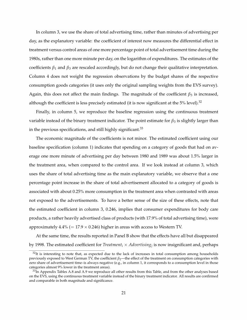
respective heights, power, and frequency of transmission; Figure 1 displays the results of our

analysis. TV signal strength (at 10 m above ground) is calculated for the whole territory of the

former GDR, divided into a raster of 1x1 km. We then calculate the average level of TV signal

strength for each municipality, based on this raster; these values range from −107 dB in Sassnitz

on the island of Rugen (northeast of the GDR) to−10.9 dB in Seeburg, on the border to West Berlin.

[Figure 1 about here]

As discussed above, for a given set of transmitters, the quality of TV signal can still vary

considerably depending on atmospheric conditions and on the power of the receiving antennas.

However, whereas above a certain level of signal strength the quality of reception does not vary

substantially with signal strength, below a certain threshold—when the noise is stronger than the

signal—no reception is possible at all. TV signal quality does not decrease linearly, but discontin-

uously, with the boundary of the discontinuity varying over time, depending among other things

on atmospheric conditions.14 To this extent, the discontinuity of TV signal strength is fuzzy.

We operationalize a definition of the treatment area based on the level of signal strength in

Dresden: existing anecdotal evidence suggests that, with normal atmospheric conditions and stan-

dard TV receiver sets, Dresden was close to the signal strength discontinuity. Only the neighbor-

hoods of Dresden located on hills were able to receive some signal under optimal conditions; the

large majority of the city’s inhabitants were not able to watch Western TV. To confirm this, we draw

on a survey of East German youths conducted in 1985, in which individuals were asked anony-

inversion.13In the overwhelming majority of East German municipalities, the strength of ARD signals was higher than for ZDF,

the second West German public TV station. We therefore focus on ARD availability. We also replicate our analysis usinginstead ZDF availability and minutes of advertising on ZDF, and the results (available upon request) are unchanged.The correlation in advertising intensity for the analyzed categories for ARD and ZDF is extremely high (ρ=0.9889).

14This is analogous to the familiar experience of listening to a radio station while driving a car: sound quality, havingbeen good for a long while, suddenly starts deteriorating, and then fades off completely.

8

mously how often they would watch Western TV stations.15 Even though this survey contains

only a rough regional indicator, referring to the district (Bezirk) of residence, the answers show

clearly the discontinuity in viewership. While in the district of Cottbus (average signal strength:

−75.9dB) only 1.67% of respondents declared that they never watched Western TV broadcasts,

in the district of Dresden (average signal strength: −86.3dB) the corresponding figure is 67.85%

(see Figure 2, top panel). The findings are reversed if one considers the percentage of respondents

watching Western TV daily (Figure 2, bottom panel).


Given that the average signal strength in the city of Dresden was −86.8 dB, we consider all

municipalities with signal strength equal or below that threshold to be in the control area. The

treatment area thus comprises all regions with a positive probability of reception of Western TV

broadcasts; note that a part of the households in the treatment area (especially those in the range

between −75 and −86.8dB) probably had no access to Western TV some or even most of the time.

The control area is thus constructed such as to comprise only individuals who, with certainty,

had no access to Western TV. In doing this, we implicitly hypothesize that all households in the

GDR area tried to watch Western TV whenever it was technically feasible, no matter how bad

the picture quality. While in contrast to studies that take signal strength as a linear predictor of

viewership (Olken, 2009; Enikolopov et al., 2011), this approach is, in our view, justified by the

crucial importance of access to Western media in a communist regime, and consistent with actual

viewership data as in Figure 2.

The resulting partition of the GDR into treatment and control areas is displayed in Figure 3.

This definition of treatment based on the geospatial modeling of signal propagation is very close

to the available anecdotal evidence on TV signal availability (cf. Figures 1 and 3 in Kern and Hain-

mueller, 2009). In our empirical analysis, we show that our results are robust to small variations

of the signal availability threshold.

15Zentralarchiv fur Empirische Sozialforschung ZA 6008. This survey was conducted by the East German Institutefor Youth Research, Zentralinstitut fur Jugendforschung. Due to the comparatively strong anonymity standards that wereapplied in conducting these surveys, they are generally considered valid sources of information—despite their prove-nance from an authoritarian regime—by most social scientists (Friedrich et al., eds, 1999; see also Kern and Hainmueller,2009, p. 381).

9


Alternatively, we also use a continuous measure of treatment, intended to replicate the actual

likelihood of Western TV viewership as a function of signal strength. We construct this measure by

fitting a (logistic) cdf to the observed viewership patterns of Figure 2, upper panel. The resulting,

S-shaped curve (a logistic cdf with parameters µ = −84.6 and σ = 2.3) is the best approximation

for the share of respondents who never watch Western TV, as a function of signal strength. Our

continuous treatment variable, representing the probability of watching any Western TV, is then

constructed by subtracting the fitted curve from unity. Figure 4 compares the binary treatment

indicator, based on the threshold at −86.8dB, and the continuous treatment variable.


3.2 Conditions for identification

For the identification strategy to be valid, we need the following four conditions to hold:

Condition 1 The inhabitants in the treatment and control regions were comparable.

While there were certainly patterns of specialization and regional peculiarities across the re-

gions of the GDR, we contend that, crucially for our identification, no substantial differences ex-

isted between the treatment and control regions as defined for the purposes of our work, neither

before the “treatment” (i.e., the regionally differentiated access to West German media) started,

nor right after reunification.

Both regions contained industrial parts, with a fairly high level of technological development

and cultural sophistication, such as Dresden in the control, Leipzig and Halle in the treatment; as

well as more agricultural and less densely populated parts, such as the control region in the North-

East around Greifswald, and the districts of Schwerin or Potsdam in the treatment. This is reflected

by the social and economic indicators reported in Table 1; these data are drawn from the GDR

Statistical Yearbooks of 1955 (the first one published after the war) and 1990. In the Yearbooks,

data are aggregated at the level of districts (Bezirk). The districts of Dresden, Neubrandenburg

and Rostock coincided partially with the regions lacking TV reception in the southeastern and

10

northeastern corner of the GDR (cf. Figures 1 and 3); we thus consider them as our “control” area,

and define the remaining 11 districts as the “treatment” area.16

As evident from the comparison in Panel A of Table 1, in the 1955 data at hand the two groups

of districts appear virtually indistinguishable with respect to the available variables: population

density, shares of employment by sector, sales and savings. Analogous data for 1990, in the last

year of the GDR’s existence, show a similar picture (Panel B). To check for differential trends be-

tween 1955 and 1990 in the two groups of districts, Panel C looks at the differences in the means of

the variables between the two years for the two groups. Again, we do not observe any significant

differences.17

[Table 1 about here]

Condition 2 No selective spatial sorting across treatment regions occurred.

It is important to exclude spatial sorting across treatment regions. If individuals more inter-

ested in Western broadcasts and/or more susceptible to Western advertising had moved into the

area with better reception, this would mar our identification of causal effects.

Before reunification. In a centrally planned economy such as the GDR, spatial mobility was se-

riously hampered; the allocation of labor as a factor of production had to follow the overarching

social and economic objectives set by the planning committees. Mobility of labor across occupa-

tions and across space was therefore considerably lower than in any free-market economy, and

was additionally reduced by the serious housing shortages that affected the GDR over the whole

40 years of its existence (Kern and Hainmueller, 2009, p. 387; Grunert, 1996).

Data based on population registries in the years 1970–1990 show that every year only 2.5 out of

100 citizens of the GDR would change their residence (or, equivalently, an average of once every

16In our baseline analysis we exclude observations from East Berlin. East Berlin was the capital of the GDR, wherea large fraction of the state bureaucracy was located, giving rise to different types of privileges to its inhabitants. Itwas a commonplace before 1990 that East Berlin’s residents never had to suffer the shortages so common in the rest ofthe GDR. Apart from that, the demographic composition of the East Berlin district is highly divergent from the otherregions, since it was mainly a city-state, seat of the country’s administration, rather than a larger territorial unit. AddingEast Berlin would therefore affect the balancedness of covariates across treatment and control areas. In our robustnessregressions, we add observations from East Berlin, and our results hold.

17In section 4, we will argue that in the context of the dataset used the treatment and control areas are balanced alonga broad array of individual-level observable covariates.

11

40 years)—a rate of spatial mobility three times lower than the corresponding value for the FRG,

a democracy and a free market economy, in the same time interval (Grundmann, 1998, p. 98).

Also, when we compare the treatment and control districts both in 1955 and 1990 (Table 1), we

do not observe any differential trend for the two groups between 1955 (before Western TV was

popular in the treatment area) and 1990 (Panel C). The two regions were very similar along the

observable variables, both before and after Western TV became a popular source of entertainment

in the treatment area.18

Between reunification and the measurement of effects. Migration of random subsets of the

populations in the treatment and control regions would attenuate our findings. However, selective

migration could potentially be a confounding factor with our estimated effects. Unfortunately, we

do not perfectly observe the type of people that migrated out of the control and treatment areas.

However, the available evidence suggests that selective migration does not seem to be of concern

in our setting. We first look at overall migration in Table 2, which shows that migration rates year

by year from treatment and control areas to West Germany were, after a peak immediately after

Reunification, comparatively low and, more importantly, statistically similar across the treatment

and control regions.19 We also provide evidence in Appendix Table A.4 that migration rates from

treatment and control regions to West Germany broken down by age intervals were essentially

identical for all age groups.


Condition 3 The individuals in East Germany that could watch West German TV did actually watch it.

Available evidence suggests that this was indeed the case. Despite the inherent danger it

would have posed to the stability of the autocratic regime, East German authorities mostly closed

18Moreover, there is no evidence for directed migration overall from the control to the treatment area. While pop-ulation declined everywhere in East Germany between 1955 and 1990, the decline was stronger in the treatment area(-9.86%) than in the control area (-6.76%).

19The largest part of East to West migration occurred in 1989 and 1990 (see Hunt, 2006); unfortunately, county-levelmigration statistics are available only for the years 1991 onwards. In Appendix A.3 we provide more detailed evidence,by analyzing total migration rates from treatment and control areas and the breakdown of these rates by destination(Berlin, West Germany, control region, and treatment region), suggesting that total migration rates were low and similarin treatment and control areas.

12

an eye on the installation of antennas suitable for watching West German TV channels. The fre-

quencies of West German TV broadcasts were not jammed, either, even though this was techni-

cally feasible and practiced in the case of radio stations (Hesse, 1988; Beutelschmidt, 1995).20 For

instance, a survey of East German youths in 1985 reported that respondents watched on aver-

age more than two hours of West Germany TV each weekday.21 As we reported in Figure 2 in

section 3.1 above, a related survey found that 66.28% of respondents in districts with access to

Western television declared they watched the Western TV stations daily. In contrast, only 5.72%

of the respondents in the district of Dresden declared so.22 Survey evidence also suggests that

Western media were used in East Germany mainly to watch entertainment shows and their ad-

vertisements (Stiehler, 2001; Buhl, 1990; Hesse, 1988).

Moreover, it was not the case that the limited availability of attractive entertainment options

and news sources in the areas without Western TV reception prompted households living there

to buy fewer TV sets. In fact, classified data from the GDR Ministry of Commerce and Provi-

sioning suggest that, in 1983, the district of Dresden had an above-average density of color TV

sets, whereas the districts of Neubrandenburg and Rostock did not differ significantly from the

country-wide average in that respect.23

Condition 4 The measured treatment effects are driven by product demand differences, and not supply

differences.

It is important that our treatment effects reflect differences in demand from the treatment and

control areas, and not differences in supply conditions. Since the regions previously not exposed

to West German television are also generally far from the border with West German, we need

to be sure that we are not capturing a “remoteness effect” that could affect the availability of

products in these areas. To address this question, we resort to the Establishment History Panel

20In 1961, after the construction of the Berlin Wall, East German authorities initially attempted to tear down roofantennas directed toward West Germany. However, the available historical evidence suggests that due to the unpop-ularity of these measures, the East German regime soon realized that it had no choice but to accept that a very largefraction of East Germans watched West German TV frequently (Kern and Hainmueller, 2009).

21Zentralarchiv fur Empirische Sozialforschung ZA 6073. Refer also to fn. 15.22Zentralarchiv fur Empirische Sozialforschung ZA 6008.23This emerges from a (then classified) report by the Institut fur Marktfortschung to the Ministry of Commerce and Pro-

visioning (Ministerium fur Handel und Versorgung): “Moglichkeiten einer naherungsweise Ermittlung von bezirklichenAusstattungs- bzw. Bestandsgroßen,” Leipzig 1983. A scan of the report is on file with the authors.

13

(Betriebs-Historik-Panel, BHP), a 50% random sample of all businesses in Germany available from

the German Institute for Employment Research (IAB). Table 3 compares the number of food super-

markets, mail order companies and other retail stores (expressed in plants per 1000 inhabitants)

active in the treatment and control areas in 1993, the first year included in our data analysis of

section 4.24 The densities of businesses are extremely similar in the two areas and the differences

are never statistically significant (the lowest p-value across the three categories is greater than

0.54). In addition to that, in subsection 4.5 we provide evidence that our measured effects are not

explained by distance to West Germany.


4 Consumption after reunification

4.1 The German Income and Expenditure Survey (EVS)

Prior to the 1990 German reunification, any differences in desired consumption choices between

individuals exposed or not to Western television could not be reflected by differences in con-

sumption behavior. Goods seen on West German TV were generally not available in communist

East Germany, where consumption was strictly regimented by the central planning operated by

the Ministry of Commerce and Provisioning. However, after reunification, such obstacle was no

longer preventing the consumption of desired goods by East Germans; any good that had been

previously seen on television could now, at least in theory, also be purchased in East Germany.

We therefore focus on the period after reunification to assess the effects of West German tele-

vision on consumption choices. For that purpose, we turn to the results of the German Income

and Expenditure Survey (Einkommens- und Verbrauchsstichprobe, EVS) conducted by the German

federal statistical office. These data can help us understand how exactly access to Western TV

changed the consumption behavior of East German citizens. Conducted every five years on over

70,000 representative households (approximately 10,000 of which are in our East German subsam-

ple), this survey records exact expenditures on a variety of goods over the course of one year.

24Results based on equivalent data for the years before 1993 are qualitatively similar and available upon request.

14

Unfortunately, the Einkommens- und Verbrauchsstichprobe is not conducted as a panel, therefore we

are not able to estimate the within-household variation during the period.25

We use the first two waves conducted after reunification: 1993 and 1998. While 1993 lies al-

ready some years after reunification, this is the first available year with data on East Germany. We

expect any effects stemming from the differential exposure to Western television before 1990 to be,

if anything, still present in 1993, while they might have already faded away by 1998, after eight

years of integration into a capitalist system.26

Table 4 provides some summary descriptive statistics, divided by treatment status (binary

treatment indicator), about the households included in the two waves of the EVS used here. In

our regressions, as well as in these summary statistics, we always use the sampling weights pro-

vided by the German federal statistical office (selection of households included in the EVS occurs

through stratified sampling). The results in Table 4 show how the treatment and control regions

are largely similar across most characteristics.


4.2 West German TV and aggregate consumption behavior

Does long-term exposure to Western television affect aggregate consumption behavior? In partic-

ular, do individuals exposed to Western television change their levels of total private consumption

and savings? Are they more likely to take on consumer credit to finance additional splurges? A

certain strand of the social science literature (Galbraith, 1958; Schor, 1998) would suggest that

advertising is used by corporations to increase households’ aspirations and overall consumption

levels.

We thus start our analysis of the effect of long-term exposure to Western television by first

25For the analyses performed in this section we had to draw on the restricted-use version of the EVS, which recordsthe municipality of residence of each household interviewed. This information is needed to determine the treatmentstatus. Due to confidentiality reasons, this version of the EVS dataset can be accessed only on the premises of theGerman statistical office (Destatis).

26In the context of preferences for redistribution and attitudes about the role of the state in society, Alesina and Fuchs-Schundeln (2007) find remarkable persistence: according to their estimates it will take about one to two generations forformer East Germans and West Germans to converge. Note, however, that, in addition to the difference in outcomevariables between the two papers, the source of divergence in our present paper is a variation within East Germany,and not between East and West.

15

examining the impact of exposure to West German TV on aggregate consumption behavior after

reunification, using the EVS data. For that purpose, we use the following regression setup:

yi = β0 + β1 Treatmenti + x′iγ + ε i, (1)

where yi are variables relating to the aggregate consumption behavior of household i, Treatmenti

is a treatment indicator equal to one for households with access to Western TV, and xi is a set of

household-level covariates, including economic and demographic characteristics (see Table 4 for

a list of covariates used in our regressions). The coefficient of interest is β1. Our main outcome

variables of interest are the log of disposable income, the log of total private consumption, and a

dummy on whether the household has positive levels of savings. We run separate regressions for

1993 and 1998.27

If households in the treatment area (those previously exposed to Western television) wanted to

consume relatively more than those in the control area, we would observe them either supplying

relatively more labor (thus increasing their incomes compared to households in the control area),

saving relatively less, or resorting relatively more to credit to finance their consumption.

Table 5 shows the treatment effects of long-term exposure to Western television on disposable

income, total private consumption, and savings. The results indicate that East German house-

holds with Western TV access before 1990 do not differ from the control group in their aggregate

behavior: the treatment effects on disposable income, total private consumption, and savings are

all statistically insignificant, both in 1993 and 1998. Moreover, all estimates can rule out even mod-

est increases in total private consumption associated with exposure to Western TV: based on the

1993 estimates (Panel A, column 2), we can rule out with 95% confidence an increase of less than

1.5% in total private consumption.


In Table 6, we look at the treatment effects on the use of financial instruments. We analyze

the effect of previous exposure to Western television on the likelihood of reporting to have taken

27Note that since the EVS is conducted as a repeated cross-section (rather than a panel) we are not able to linkhouseholds across waves.

16

consumer credit and to have overdraft payments on a checking account, using a linear probability

model. If households in the treatment area felt a comparatively stronger need to buy the con-

sumption goods seen on Western television after they suddenly became available in 1990, they

could have resorted to consumer credit or overdraft on bank accounts to finance those purchases.

Repayment of these credits would then still be visible in 1993. However, the absence of significant

treatment effects in the regressions of Table 6 does not corroborate this hypothesis. Here, too, the

estimates are precise enough to rule out meaningful quantities: in 1993, we can rule out with 95%

confidence a propensity to resort to consumer credit that is 6% higher in the treated regions, and

a propensity to resort to overdraft that is 1% higher.


The general picture is therefore one of lack of effects on aggregate consumption behavior. Un-

fortunately, we cannot address whether this is due to previous exposure to West German television

truly not affecting post-reunification aggregate consumption, the effects having already vanished

in 1993, or households being constrained in their ability to adjust aggregate consumption behav-

ior. Yet, the absence of effects on aggregate variables does not preclude an alternative kind of

effect: long-term exposure to West German television could have affected the composition of con-

sumption after reunification, shifting consumption towards some particular categories of goods.

4.3 West German TV advertising and the composition of consumption

We expect advertising to be an important channel through which Western television might impact

consumption choices. To study how advertising, present in West German television but not in East

German broadcasts, affected post-reunification composition of consumption, we use data about

the quantity of advertising (measured in minutes) on West German TV stations between 1980

and 1989 (Zentralausschuss der Werbewirtschaft, ed., 1980-1989). Table 7 lists categories of goods

ranked by the percentage of total minutes of advertising on the main West German TV channel,

ARD. Food and drinks as well as body care products make up the largest part of advertising on

television, whereas other categories of goods, such as clothing or tourism, make up for a much

17

smaller share of total advertising time.28


The effects of advertising on consumption patterns could conceivably take different forms. Ex-

posed households could consume more of the more heavily advertised brands of a given product,

preferring them to “no-name” items. This would correspond to having a higher brand-recognition

factor for advertised goods among East German citizens who had watched Western television pre-

viously. With the data available to us, we are not able to test this hypothesis; both the advertising

figures in Table 7 and the categories of consumption goods in the EVS are not detailed up to the

level of brands. Here, rather than focusing on shifts across brands, we examine whether house-

holds spend more on categories of goods that, according to the figures of Table 7, were more heavily

advertised on television to the detriment of those categories of consumption goods that were less

advertised.29 We matched the items recorded in the EVS surveys to the categories of Table 7.

Other types of consumption goods present in the exhaustive catalog of the EVS are not present at

all among the goods advertised on television: e.g., expenditures for house rental, utilities, bicycles,

or telephones. For those goods, we created an eleventh category corresponding to all goods with

zero share of advertising time.

To first visualize the effects of Western television advertising on consumption choices, we ex-

amine Figures 5 and 6, which display the logarithm of raw differences between treatment and

control regions in average yearly consumption levels by categories of consumption. The cate-

gories of consumption goods are sorted along the horizontal axis according to their shares of total

advertising time averaged over the period 1980-1989, as in Table 7. Each figure also plots a lin-

ear fit of the raw data, weighting categories of consumption by their budget share. We choose

to weight regressions according to the budget shares of the goods categories in order not to give

28Note that the overall amount of advertising on the state television broadcasting stations was low, totaling less than20 minutes per day on average. These amounts, as well as the times of the day in which advertising was allowed, wereregulated by law (Rundfunkstaatsvertrag of 1987, §3). Most of the advertising occurred in the “prime time” between 7and 8pm.

29The question whether advertising is, within categories of goods, “predatory” (i.e., one brand advertises at thedetriment of the other brands) or “cooperative” (advertising increases overall sales) has been discussed in the industrialorganization literature. See, for example, Rojas and Peterson (2008) for the beer industry. In the context of our study,we would find any effects only if advertising was cooperative within goods categories.

18

undue weight to categories that are considered separately in the (arguably arbitrary) classification

of the German advertising statistics, but have little importance in most households’ budgets: e.g.,

the category “Photo, optics, watches, jewelry,” which makes up for only 1.1% of the budget of the

average household in 1993 (see Table 7, third column).



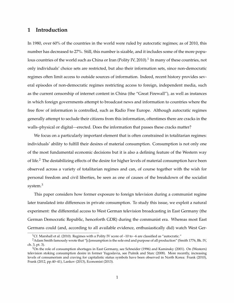
The figures suggest that in 1993 (Figure 5), higher intensity of advertising was associated with

(significantly) larger consumption in the treatment areas compared to the control areas. The slope

of the line is 0.0024 with an associated t-statistic of 2.20. On average, most categories of consump-

tion goods display a negative difference between treatment and control area; this is consistent with

the negative (but not significant) effect of treatment status on total private consumption (Table 5,

Panel A, column 2). In 1998 (Figure 6), the effects seem to have vanished, with a slope of 0.0003

(and a t-statistic of 0.25).

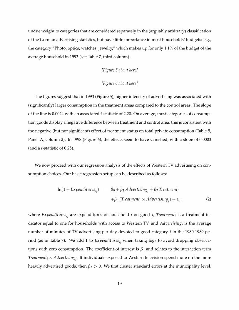
We now proceed with our regression analysis of the effects of Western TV advertising on con-

sumption choices. Our basic regression setup can be described as follows:

ln(1 + Expendituresij) = β0 + β1 Advertisingj + β2 Treatmenti

+β3 (Treatmenti × Advertisingj) + ε ij, (2)

where Expendituresij are expenditures of household i on good j, Treatmenti is a treatment in-

dicator equal to one for households with access to Western TV, and Advertisingj is the average

number of minutes of TV advertising per day devoted to good category j in the 1980-1989 pe-

riod (as in Table 7). We add 1 to Expendituresij when taking logs to avoid dropping observa-

tions with zero consumption. The coefficient of interest is β3 and relates to the interaction term

Treatmenti × Advertisingj. If individuals exposed to Western television spend more on the more

heavily advertised goods, then β3 > 0. We first cluster standard errors at the municipality level.

19

In our baseline specification, regressions are weighted both by the EVS sampling weights and by

the budget share of each category of consumption goods.

Alternatively, we can add a set of household-level covariates xi (as in the previous section of

the paper):

ln(1 + Expendituresij) = β0 + β1 Advertisingj + β2 Treatmenti

+β3 (Treatmenti × Advertisingj) + x′iγ + ε ij, (3)

The inclusion of household-level covariates does not affect the point estimates β1 or β3 since

Advertisingj does not vary at the household level, and the effect of Treatmenti at the household

level is captured by β2. Conditional on Advertisingj and Treatmenti, the interaction term of these

variables is orthogonal to covariates xi that vary only at the household level.

Table 8 presents the results of estimating our regression model (2), once for the 1993 EVS survey

(Panel A) and once with the 1998 data (Panel B). In column 1, we present the results following the

setup in equation 2, and in column 2 we show the results associated with the baseline specification

adding household-level covariates, as in equation 3. The coefficient on intensity of advertisement,

β1 shows that, in the control region, categories of goods with more advertising are associated with

higher expenditures.30 The direct effect of a household’s location in the treatment area, β2, is neg-

ative but not significant; note that this corresponds to the direct effect in the case of a category of

goods with zero advertising. As one moves to goods categories with a higher intensity of adver-

tising, households in the treatment group consume more than those in the control region. This

can be derived from the fact that the coefficient on the interaction term Treatmenti × Advertisingj,

β3, is positive and significant at the 1% level. Note that, as predicted, the inclusion of household

covariates in column 2 only affects the point estimate of β2.31

[Table 8 about here]30This is expected, since some categories with high intensity of advertising (e.g., food) are large items in household

budgets. The coefficient β1 cannot be interpreted as a (causal) effect of advertising on consumption.31Analogously, including a full set of interaction terms between the treatment dummy and household covariates

would not affect the point estimate of the interaction term, β3.

20

In column 3, we use the share of total advertising time, rather than minutes of advertising per

day, as the explanatory variable: the coefficient of interest now measures the differential effect in

treatment versus control areas of one more percentage point of total advertisement time during the

1980s, rather than one more minute per day, on the logarithm of expenditures. The estimates of the

coefficients β1 and β3 are rescaled accordingly, but do not change their qualitative interpretation.

Column 4 does not weight the regression observations by the budget shares of the respective

consumption goods categories (it uses only the original sampling weights from the EVS survey).

Again, this does not affect the main findings. The magnitude of the coefficient β3 is increased,

although the coefficient is less precisely estimated (it is now significant at the 5% level).32

Finally, in column 5, we reproduce the baseline regression using the continuous treatment

variable instead of the binary treatment indicator. The point estimate for β3 is slightly larger than

in the previous specifications, and still highly significant.33

The economic magnitude of the coefficients is not minor. The estimated coefficient using our

baseline specification (column 1) indicates that spending on a category of goods that had on av-

erage one more minute of advertising per day between 1980 and 1989 was about 1.5% larger in

the treatment area, when compared to the control area. If we look instead at column 3, which

uses the share of total advertising time as the main explanatory variable, we observe that a one

percentage point increase in the share of total advertisement allocated to a category of goods is

associated with about 0.25% more consumption in the treatment area when contrasted with areas

not exposed to the advertisements. To have a better sense of the size of these effects, note that

the estimated coefficient in column 3, 0.246, implies that consumer expenditures for body care

products, a rather heavily advertised class of products (with 17.9% of total advertising time), were

approximately 4.4% (= 17.9× 0.246) higher in areas with access to Western TV.

At the same time, the results reported in Panel B show that the effects have all but disappeared

by 1998. The estimated coefficient for Treatmenti × Advertisingj is now insignificant and, perhaps

32It is interesting to note that, as expected due to the lack of increases in total consumption among householdspreviously exposed to West German TV, the coefficient β2—the effect of the treatment on consumption categories withzero share of advertisement time–is always negative (e.g., in column 1, it corresponds to a consumption level in thosecategories almost 9% lower in the treatment areas).

33In Appendix Tables A.8 and A.9 we reproduce all other results from this Table, and from the other analyses basedon the EVS, using the continuous treatment variable instead of the binary treatment indicator. All results are confirmedand comparable in both magnitude and significance.

21

more importantly, clearly smaller in magnitude across all specifications. For example, in our base-

line specification of column 1, the effect declines to about one seventh of the size measured for

1993.

Another way to appreciate the magnitudes of the estimated effects is to gauge how large the

likely effect was just after reunification; recall that the results of Panel A stem from the survey

conducted in 1993, three years after the East was integrated into the West German economy and

all households in the former GDR were exposed to the same TV stations and had access to the

same types of goods. As a back-of-the envelope calculation, assume that the treatment effect of

exposure to Western television and its advertising content declines linearly over time. In that

case, the decline witnessed between 1993 and 1998 for the specification of column (1) corresponds

to a hypothetical effect of 2.341 in 1990, the year of German reunification: that is, an effect of

approximately 2.3% more consumption expenditures for every additional minute of television

advertising time on average between 1980 and 1989 spent on a given category of goods.34

It is important to note that our results are robust to dropping single categories of consumption

goods one at a time, as displayed in Appendix Table A.7. The only case in which our coefficient

of interest (β3) is no longer significant in 1993 is when we drop the Food, drinks category. The

point estimate for β3 is actually 25% larger when we drop that category (compared to our baseline

specification), indicating that the category is not an outlier. We lose precision when dropping that

category since it is the most important category in in terms of its budget share in 1993 (accounting

for 23.7% of the budget). Since we weigh regressions by the budget share of each category, drop-

ping the Food, drinks category implies a large reduction in our effective sample size, thus reducing

the precision of our estimates.

As a whole, the regression results draw a picture in which East German households in the

treatment areas (i.e., with access to Western television until 1990) are particularly susceptible to

pre-reunification advertising when making the choice between different categories of consump-

tion goods in the early post-reunification period.

34The persistence of the effect of advertising of the 1980s into the 1990s is even more remarkable if one considers thatthe marketing literature (Lodish et al., 1995) finds that the carryover effect of advertising is about 6 to 9 months, and iseven weaker in absence of reinforcement through actual purchases (Givon and Horsky, 1990).

22

4.4 Robustness checks: Changing samples, clustering, treatment definition

Table 9 presents further robustness checks, departing from the baseline regression of Table 8, col-

umn 1 (budget shares weights, binary treatment indicator, no household covariates). In column 1,

we reproduce the regressions clustering at the household level, rather than at the municipality

level, as in Table 8. All standard errors are now smaller than before, suggesting that clustering

at the municipality level, by taking into account the correlation across households in the same

municipality, is the more conservative approach.35

In column 2, we include observations from East Berlin, which were originally dropped in Table

8. Again, all findings are virtually unchanged. In columns 3–5, we vary our definition of thresh-

old for availability of West German TV broadcasts (by 2dB each time to −84.8dB, −82.8dB, and

−80.8dB) to see if our findings are robust to variations on the level of signal strength that defines

treatment and control.36 The coefficients of interest in columns 3–5 are similar to the baseline

coefficients from column 1 in Table 8 and are also significant at the 1% level.

Just as before, the effects are much smaller and no longer significant in 1998, as observed in

Panel B of Table 9.


In Table 10, we proceed with a different set of robustness checks. Instead of varying the defi-

nition of our threshold of signal availability, as in Table 9, we now restrict our areas of analysis to

regions with West German TV signal strength sufficiently close to our original threshold of signal

availability. This approach is in the spirit of a regression-discontinuity design, although we do

not have a clear discontinuity in signal availability. We restrict the analysis to regions in which

the signal strength is within 30dB (column 1), 20dB (column 2), or 10dB (column 3) of the original

−86.8dB threshold..37 In the first two settings, our results hold and are quantitatively very similar

to the baseline results from Table 8 In Table 10, Panel B, we observe that the results have either

decreased or disappeared by 1998.35In Appendix Table A.6, we show that our results are robust to aggregating households into larger clusters.36We do not change the threshold in the other direction, since that would assign the entire municipality of Dresden—

which was known to have virtually no access to Western television broadcasts—to the treatment area.37See the Supplemental Appendix, Tables A.10–A.12, for a comparison of household covariates in the treatment and

control areas under the three different sample restrictions criteria of Table 10.

23

If we further restrict our sample to regions in which the signal strength is within 10dB of the

original threshold, our results no longer hold, as observed in column 3 of Table 10. This is not

surprising in the light of the survey evidence presented in Figure 2, which suggests that the dis-

continuity threshold lay approximately between−75 and−86dB. Since the discontinuity in access

to West German TV signals is not sharp, many individuals in the “treatment” area within 10 dB

of the original threshold would most likely not have access to the broadcasts on a everyday basis,

either. In practice, in the sample restricted to −86.8± 10dB one would be comparing individuals

with no exposure to West German TV with individuals with very little exposure to West German

TV, thus attenuating our findings.


4.5 The effect of distance to West Germany

An alternative explanation for the findings of the previous subsection could be that such results

are simply the product of the control areas’ distance from the West German border. Such longer

distance could make the access to Western goods more difficult, increase the time that Western

goods take to penetrate the local market, among other plausible factors that could affect consump-

tion choices. Although we have no reason to think that the goods that were less likely to penetrate

the local market in the control areas were also the ones with higher intensity of advertising, it is

important to address that alternative explanation. To examine that, in Table 11, we reproduce our

main analysis adding as a covariate the minimum driving distance (in kilometers) between any

household’s municipality of residence in our data set and the closest point in former West Ger-

many (including the exclave of West Berlin). To compute this variable, we used the actual East

German road and highways network as of 1990.

Having the explanatory variable “availability of West German TV broadcasts” compete with

the shortest distance to either the West German border or West Berlin makes for a strong test of

our hypotheses: the effects will thus only be identified from those cases where geographic features

of the landscape do not reduce travel distance but prevent TV signals to reach the households

in the survey. The empirical setup chosen corresponds to equation (2); however, in addition to

24

the interaction of interest Treatmenti × Advertisingj, we include a further variable representing

the interaction between the intensity of advertising and distance to West Germany: Distancei ×

Advertisingj.38


The results in column 1 show that the main coefficient of interest is entirely unaffected by the

inclusion of the distance measure. This makes us confident that the estimated effects stem, in fact,

from differential access to West German broadcasts before 1990, and not merely from distance to

West German markets.

An alternative way to assess the potentially confounding effect of distance is to run placebo

regressions restricting our sample to the treatment region only, where Western TV signal was

available before 1990. If distance, and not access to Western TV, explained the difference of con-

sumption patterns, this effect should be visible also when considering the variation within the

treatment region only, i.e. among those households that had access to Western TV throughout.

Here we use interaction of distance to West Germany with advertising time as the explanatory

variable of interest. As shown in column 2 of Table 11, distance to West Germany does not explain

the differences in consumption choices within the region with access to Western broadcasts.

5 Conclusion

We study the impact of long-term exposure to Western television on consumption behavior ex-

ploiting a setting with plausibly exogenous variation of the explanatory variable: differential ac-

cess to Western television in former East Germany, a variation that was mainly determined by

geographic features.

While our data do not support the hypothesis that Western television shifts aggregate con-

sumption patterns (total private consumption, savings), we provide evidence consistent with

Western television affecting the composition of consumption through advertising. Expenditures

38We also reproduce tables 5 and 6 (i.e., the regressions relating to aggregate consumption behavior from section4.2) adding our distance to West Germany variable, and the coefficient of interest (on the treatment indicator) alwayscontinues to be insignificant. Results are available from the authors upon request.

25

on categories of goods with higher shares of advertising time on pre-reunification Western tele-

vision were, after 1990, higher in the areas reached by Western broadcasts. Our unique setting

allows for a well-identified analysis of the causal impact of long-term exposure to advertising on

consumption behavior, since the East Germans that could watch West German broadcasts were

not the targeted audience of the advertising.

Our findings also suggest that television advertising changes consumption patterns in a way

that is more than just to induce individuals to switch across brands of the same good. Advertising

may induce a recomposition of consumption across broad categories of goods, depending on the

amount of advertising for each category.

26

References

Alesina, Alberto and Nicola Fuchs-Schundeln, “Good Bye Lenin (or Not?): The Effect of Com-munism on People’s Preferences,” American Economic Review, 2007, 97 (4), 1507–1528.

Avery, Rosemary, Donald Kenkel, Dean Lillard, and Alan Mathios, “Private Profits and PublicHealth: Does DTC Advertising of Smoking Cessation Products Encourage Smokers to Quit?,”Journal of Political Economy, 2007, 115 (3), 447–481.

Bagwell, Kyle, “The Economic Analysis of Advertising,” in Mark Armstrong and Rob Porter, eds.,Handbook of Industrial Organization, Vol. 3, Amsterdam: North-Holland, 2007, pp. 1701–1844.

Baker, Matthew J. and Lisa M. George, “The Role of Television in Household Debt: Evidencefrom the 1950’s,” The BE Journal of Economic Analysis & Policy, 2010, 10 (1), 1–36.

Becker, Gary S. and Kevin M. Murphy, “A Simple Theory of Advertising as a Good or Bad,”Quarterly Journal of Economics, November 1993, 108 (4), 941–964.

Benhabib, Jess and Alberto Bisin, “Advertising, Mass Consumption and Capitalism,” February2002. Unpublished manuscript, NYU.

Beutelschmidt, Thomas, Sozialistische Audiovision, Vol. 3 of Veroffentlichungen des Deutschen Rund-funkarchivs, Potsdam: Verlag fur Berlin-Brandenburg, 1995.

Bronnenberg, Bart, Jean-Pierre Dube, and Matthew Gentzkow, “The Evolution of Brand Prefer-ences: Evidence from Consumer Migration,” February 2011. Unpublished manuscript, Univer-sity of Chicago.

Buhl, Dieter, “Window to the West: How Television from the Federal Republic Influenced Eventsin East Germany,” 1990. Discussion paper D-5, Joan Shorenstein Barone Center, Harvard Uni-versity.

Burchardi, Konrad B. and Tarek A. Hassan, “The Economic Impact of Social Ties: Evidence fromGerman Reunification,” NBER Working Paper, June 2011, 17186.

Cameron, A. Colin, Jonah B. Gelbach, and Douglas L. Miller, “Bootstrap-based Improvementsfor Inference with Clustered Errors,” Review of Economics and Statistics, August 2008, 90 (3), 414–427.

Chang, Chun-Fang and Brian Knight, “Media Bias and Influence: Evidence from NewspaperEndorsements,” 2011. Forthcoming, Review of Economic Studies.

Claus, Werner, ed., Medien-Wende, Wende-Medien? Dokumentation des Wandels im DDR- Journalis-mus, Berlin: Vistas, 1991.

DellaVigna, Stefano and Ethan Kaplan, “The Fox News Effect: Media Bias and Voting,” QuarterlyJournal of Economics, August 2007, 122 (3), 1187–1234.

and Matthew Gentzkow, “Persuasion: Empirical Evidence,” Annual Review of Economics, 2010,2, 643–669.

27

, Ruben Enikopolov, Vera Mironova, Maria Petrova, and Ekaterina Zhuravskaya, “Unin-tended Media Effects in a Conflict Environment: Serbian Radio and Croatian Nationalism,”NBER Working Paper, May 2011, 16989.

Dixit, Avinash K. and Victor Norman, “Advertising and Welfare,” Bell Journal of Economics, Spring1978, 9 (1), 1–17.

Economist, “North Korea: Rumblings from below,” 2013. Feb 9.

Enikolopov, Ruben, Maria Petrova, and Ekaterina Zhuravskaya, “Media and Political Persua-sion: Evidence from Russia,” American Economic Review, 2011, 111 (7), 3253–3285.

Frank, Rudiger, “Money in Socialist Economies: The Case of North Korea,” The Asia-Pacific Jour-nal, February 22, 2010, 8-2-10.

, “North Korea in 2011: Domestic Developments and the Economy,” in Rudiger Frank, James E.Hoare, Patrick Kollner, and Susan Pares, eds., Korea 2012: Politics, Economy and Society, Leiden:Brill, 2012, pp. 39–64.

Friedrich, Walter, Peter Forster, and Kurt Starke, eds, Das Zentralinstitut fur JugendforschungLeipzig 1966–1990, Berlin: Edition Ost, 1999.

Friehe, Tim and Mario Mechtel, “Conspicuous Consumption and Communism: Evidence fromEast and West Germany,” CESifo Working Paper Series, 2012, 3922.

Galbraith, John Kenneth, The Affluent Society, Boston: Houghton Mifflin, 1958.

Gentzkow, Matthew, “Television and Voter Turnout,” Quarterly Journal of Economics, 2006, 121,931–972.

and Jesse Shapiro, “Media, Education and Anti Americanism in the Muslim World,” Journal ofEconomic Perspectives, 2004, 18 (3), 117–133.

Gerber, Alan S., Dean Karlan, and Daniel Bergan, “Does the Media Matter? A Field ExperimentMeasuring the Effect of Newspapers on Voting Behavior and Political Opinions,” American Eco-nomic Journal: Applied Economics, 2009, 1 (2), 35–52.

Givon, Moshe and Dan Horsky, “Untangling the effects of purchase reinforcement and advertis-ing carryover,” Marketing Science, 1990, 9 (2), 171–187.

Grundmann, Siegfried, Bev”olkerungsentwicklung in Ostdeutschland, Opladen: Leske+Budrich,1998.

Grunert, Holle, “Das Beschaftigungssystem der DDR,” in Burkart Lutz, Hildegard M. Nickel,Rudi Schmidt, and Arndt Sorge, eds., Arbeit, Arbeitsmarkt und Betriebe, Opladen: Leske+Budrich,1996.

Hesse, Kurt R., Westmedien in der DDR, Koln: Verlag Wissenschaft und Politik, 1988.

Hu, Ye, Leonard M. Lodish, and Abba M. Krieger, “An analysis of real world TV advertisingtests: A 15-year update,” Journal of Advertising Research, 2007, 47 (3), 341.

28

Hufford, George A., “The ITS Irregular Terrain Model, version 1.2.2.: The Algorith,” 1995. mimeo,National Telecommunications and Information Administration, Institute for Telecommunica-tion Sciences, Boulder, Colo.

Hunt, Jennifer, “Staunching Emigration from East Germany: Age and the Determinants of Mi-gration,” Journal of the European Economic Association, 2006, 4 (5), 1014–1037.

Jensen, Robert and Emily Oster, “The Power of TV: Cable Television and Women’s Status inIndia,” Quarterly Journal of Economics, 2009, 143 (3), 1057–1094.

Kaminsky, Annette, Wohlstand, Schonheit, Gluck: Kleine Konsumgeschichte der DDR, Munchen: C.H.Beck, 2001.

Kern, Holger Lutz and Jens Hainmueller, “Opium for the Masses: How Foreign Media CanOpium for the Masses: How Foreign Media Can Stabilize Authoritarian Regimes,” PoliticalAnalysis, 2009, 17, 377–399.

La Ferrara, Eliana, Alberto Chong, and Suzanne Duryea, “Soap Operas and Fertility: Evidencefrom Brazil,” American Economic Journal: Applied Economics, 2012, forthcoming.

Lankov, Andrei, “Low-Profile Capitalism: The Emergence of the New Merchant/EntrepreneurialClass in Post-Famine North Korea,” in Kyung-Ae Park and Scott Snyder, eds., North Korea inTransition, Lanham, Md.: Rowman & Littlefield, 2013, chapter 8, pp. 197–194.

Lodish, Leonard M., Moshe M. Abraham, Jeanne Livelsberger, Beth Lubetkin, B. Richardson,and Mary Ellen Stevens, “A summary of fifty-five in-market experimental estimates of thelong-term effect of TV advertising,” Marketing Science, 1995, 14 (3 supplement), G133–G140.

Marshall, Monty G., Keith Jaggers, and Ted Robert Gurr, “Polity IV Project: Political RegimeCharacteristics and Transitions, 1800–2010,” 2010. Center for Systemic Peace.

Milgrom, Paul and John Roberts, “Price and Advertising Signals of Product Quality,” Journal ofPolitical Economy, 1986, 94 (4), 796–821.

Muller, Susanne, Von der Mangel- zur Marktwirtschaft, Leipzig: mimeo, IM Leipzig, 2000.

Nelson, Phillip, “Advertising as Information,” Journal of Political Economy, 1974, 82 (4), 729–754.

Norddeutscher Rundfunk, ed., Horfunk und Fernsehsender in der Bundesrepublik Deutschland ein-schließlich Berlin (West) nach dem Stand vom 1. Januar 1989, Wedel (Holstein): NorddeutscherRundfunk, 1989.

Olken, Benjamin A., “Do TV and Radio Destroy Social Capital? Evidence from Indonesian Vil-lages,” American Economic Journal: Applied Economics, 2009, 1 (4), 1–33.

Pusnik, Marusa and Gregor Starc, “An entertaining (r)evolution: the rise of television in socialistSlovenia,” Media, Culture & Society, 2008, 30 (6), 777–793.

Putman, Robert D., Bowling alone: the collapse and revival of American community, New York: Simon& Schuster, 2000.

29

Rojas, Christian and Everett B. Peterson, “Demand for differentiated products: Price and adver-tising evidence from the US beer market,” International Journal of Industrial Organization, 2008,26 (1), 288–307.

Schneider, Gernot, “Lebensstandard und Versorgungslage,” in Eberhart Kuhrt, Hannsjorg F.Buck, and Gunter Holzweißig, eds., Die wirtschaftliche und okologische Situation der DDR in den80er Jahren, Vol. 2 of Am Ende des realen Sozialismus, Opladen: Leske+Budrich, 1996, pp. 111–136.

Schor, Juliet B., The Overspent American: Upscaling, Downshifting, and the New Consumer, New York:Basic Books, 1998.

Sethuraman, Raj, Gerard J. Tellis, and Richard A. Briesch, “How well does advertising work?generalizations from meta-analysis of brand advertising elasticities,” Journal of Marketing Re-search, 2011, 48 (3), 457–471.

Sinn, Gerlinde and Hans-Werner Sinn, Jumpstart: The Economic Unification of Germany, Cam-bridge, Mass.: MIT Press, 1992.

Smith, Adam, An Inquiry into the Nature and Causes of the Wealth of Nations, New York: ModernLibrary, 1776/2000.

Snyder, Jim and David Stromberg, “Press Coverage and Political Accountability,” Journal of Po-litical Economy, 2008, 118 (2), 355–408.

Statistisches Amt der DDR, ed., Statistisches Jahrbuch der Deutschen Demokratischen Republik,Berlin: VEB Deutscher Zentralverlag, (various years).

Stiehler, Hans-Jurgen, Leben ohne Westfernsehen, Leipzig: Leipziger Universitatsverlag, 2001.

Stromberg, David, “Radio’s Impact on Public Spending,” Quarterly Journal of Economics, 2004, 119(1), 189–221.

Wind, Yoram and Byron Sharp, “Advertising Empirical Generalizations: Implications for Re-search and Action,” Journal of Advertising Research, 2009, 49 (2), 246.

Yanagizawa-Drott, David, “Propaganda and Conflict: Theory and Evidence From the RwandanGenocide,” 2010. Unpublished, Harvard Kennedy School.

Zentralausschuss der Werbewirtschaft, ed., Werbung in Deutschland, Bonn: Zentralausschuss derWerbewirtschaft, (various years).

30

Figures and Tables

Figure 1: Signal strength (ARD) in East Germany, 1989. Dark: weak signal. (Yellow) dots representmajor cities. District borders (Bezirke) superimposed as white lines.

31

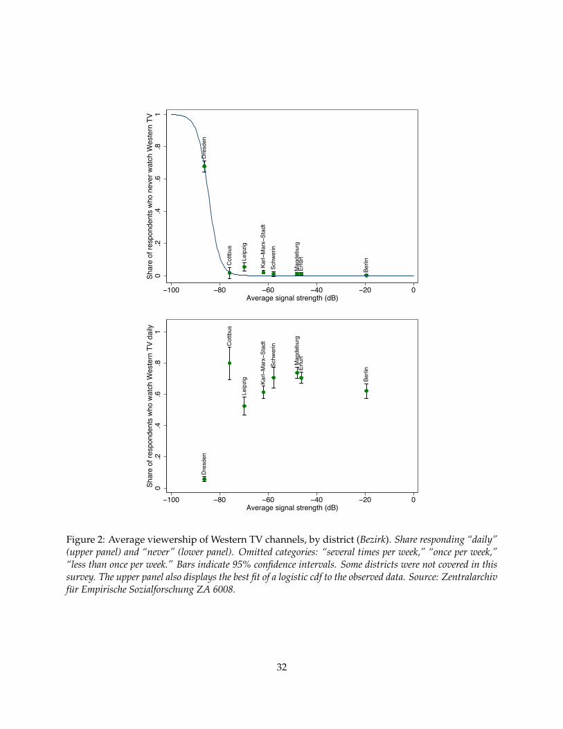
Sch

wer

in

Mag

debu

rg

Berli

n

C

ottb

us

Lei

pzig

D

resd

en

Kar

lM

arx

Stad

t

Erfu

rt

0.2

.4.6

.81

Shar

e of

resp

onde

nts

who

nev

er w

atch

Wes

tern

TV

100 80 60 40 20 0Average signal strength (dB)

S

chw

erin

M

agde

burg

B

erlin

C

ottb

us

L

eipz

ig

Dre

sden

Ka

rlM

arx

Stad

t

Er

furt

0.2

.4.6

.81

Shar

e of

resp

onde

nts

who

wat

ch W

este

rn T

V da

ily

100 80 60 40 20 0Average signal strength (dB)

Figure 2: Average viewership of Western TV channels, by district (Bezirk). Share responding “daily”(upper panel) and “never” (lower panel). Omitted categories: “several times per week,” “once per week,”“less than once per week.” Bars indicate 95% confidence intervals. Some districts were not covered in thissurvey. The upper panel also displays the best fit of a logistic cdf to the observed data. Source: Zentralarchivfur Empirische Sozialforschung ZA 6008.

32

Figure 3: Signal strength (ARD) in East Germany, 1989. Dark: Signal strength below –86.7dB (thresh-old based on signal availability in Dresden). (Yellow) dots represent major cities. District borders (Bezirke)superimposed as white lines.

33

0.2

.4.6

.81

Trea

tmen

t

100 80 60 40 20ARD signal strength (dB)

Figure 4: Treatment definitions. The figure compares the binary treatment definition, based on the thresh-old of –86.7dB, and the continuous treatment definition, based on the fit of actual viewership data as inFigure 2, upper panel.

34

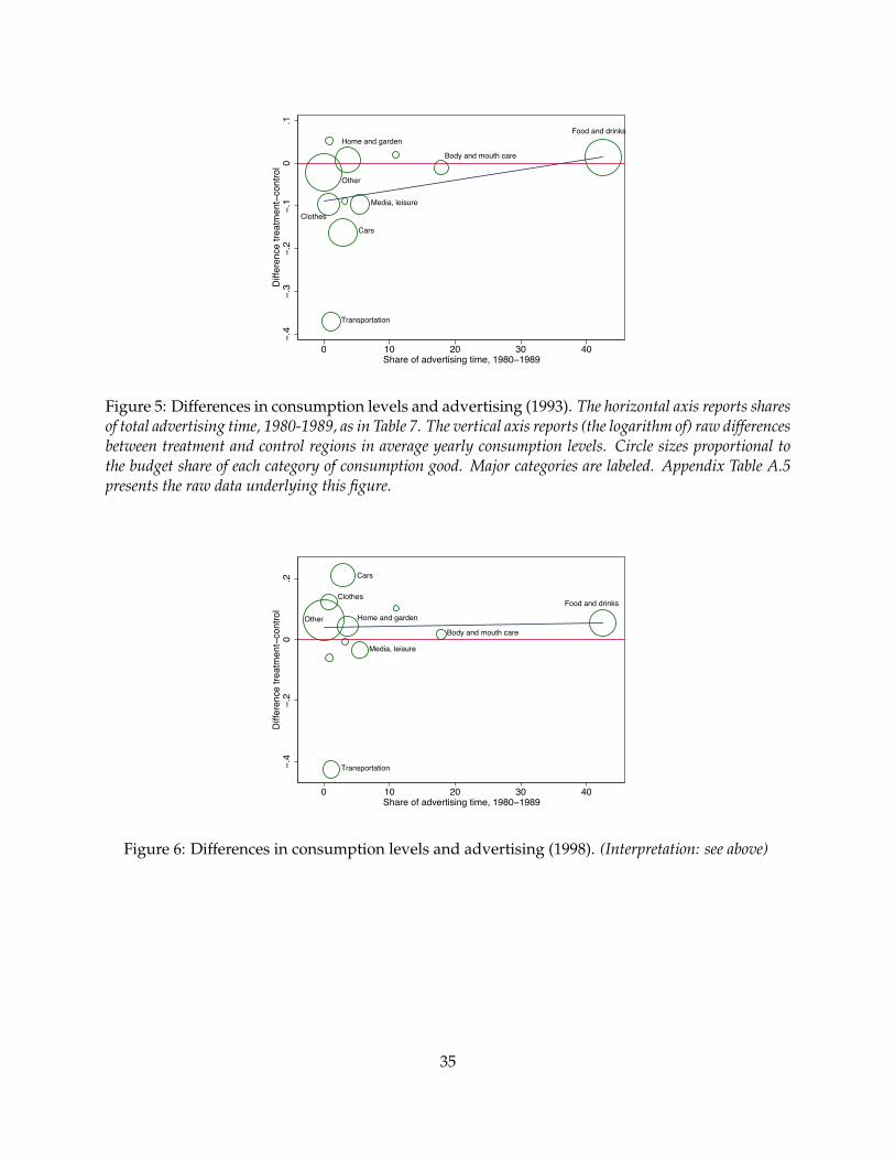
Food and drinks

Transportation

Cars

Other

Home and garden

Body and mouth care

Media, leisure

Clothes

−.4

−.3

−.2

−.1

0.1

Diffe

renc

e tre

atm

ent−

cont

rol

0 10 20 30 40Share of advertising time, 1980−1989

Figure 5: Differences in consumption levels and advertising (1993). The horizontal axis reports sharesof total advertising time, 1980-1989, as in Table 7. The vertical axis reports (the logarithm of) raw differencesbetween treatment and control regions in average yearly consumption levels. Circle sizes proportional tothe budget share of each category of consumption good. Major categories are labeled. Appendix Table A.5presents the raw data underlying this figure.

Food and drinks

Body and mouth care

Media, leisure

Home and garden

Cars

Clothes

Other

Transportation−.4

−.2

0.2

Diffe

renc

e tre

atm

ent−

cont

rol

0 10 20 30 40Share of advertising time, 1980−1989

Figure 6: Differences in consumption levels and advertising (1998). (Interpretation: see above)

35

Table 1: Regional characteristics 1955 and 1990 (district level), by treatment status

Treatment Control Diff. Std. err. p-value

Panel A: 1955 (district level data)

Population density (inhab./km2) 206 202 4 77 0.959Share of employed in agriculture (%) 23.7 27.8 -4.1 11.1 0.744Share of employed in industry (%) 34.1 28.7 5.4 10.0 0.635Retail sales per capita (Mark) 1691 1694 -3 102 0.979Savings per capita (Mark) 277 297 -20 28 0.544

Panel B: 1990

Population density (inhab./km2) 181 176 5 62 0.941Share empl. in agriculture (%) 13.5 11.3 2.2 5.1 0.706Share empl. in industry (%) 33.2 39.5 -6.3 7.5 0.479Retail sales p.c. (Mark) 7577 7250 327 188 0.190Savings p.c. (Mark) 9312 9381 -69 928 0.946Cars per 1000 inhab. 237.4 237.6 -0.2 12.1 0.992

Panel C: Difference 1990–1955

Population density (inhab./km2) -18 -26.2 8.2 15.4 0.626Share empl. in agriculture (%) -14.5 -12.6 -1.9 6.0 0.778Share empl. in industry (%) 5 5.5 -0.5 3.0 0.870Retail sales p.c. (Mark) 5862 5557 305 157 0.142Savings p.c. (Mark) 8946 8994 -48 770 0.954

Population-weighted averages, excluding the district of East Berlin. P-values based onweighted Welch’s t-tests of difference in means (two-sided, allowing for unequal variances).Total number of districts: 14 (11 treatment, 3 control). Source: Statistisches Amt, ed, Statis-tisches Jahrbuch der DDR, 1955 and 1990.

Table 2: Migration rates 1991–1993 (county level), by treatment status

Variable Treatment Control Diff. Std. err. p-value

Migration rate to West Germany (%), 1991 0.368 0.343 0.024 0.034 0.480Migration rate to West Germany (%), 1992 0.572 0.566 0.006 0.028 0.845Migration rate to West Germany (%), 1993 0.596 0.607 -0.011 0.029 0.704

Total number of counties (Kreise): 215 (192 treatment, 23 control). P-values based on t-tests ofdifference in means, allowing for unequal variances. Source: own analysis based on migrationmatrices (by Kreis), German Federal Statistical Office.

36

Table 3: Supply side: Differences across treatment regions, 1993 (county level)

Variable Treatment Control Diff. Std. err. p-value

Food supermarkets 0.075 0.070 0.004 0.015 0.782Mail order companies 0.011 0.011 -0.001 0.002 0.844Other retail stores 1.767 1.715 0.052 0.083 0.544

Variables are expressed as number of plants per 1000 inhabitants. Total num-ber of counties (Kreise): 86 (75 treatment, 11 control). P-values based on t-testsof difference in means, allowing for unequal variances. Source: own analysisbased on the IAB Establishment History Panel (Betriebs-Historik-Panel, BHP)

Table 4: Balancedness of covariates, EVS

Variable Treatment Control Diff. Std. Err. p-value

Panel A: EVS 1993

Disposable Income 41268.8 41676.4 -407.6 1028.6 0.692Age 50.1 47.9 -2.2 1 0.028N. of Children 0.659 0.787 -0.127 0.045 0.005Single 0.282 0.246 0.036 0.023 0.125Female 0.422 0.43 -0.008 0.025 0.759German 0.997 0.998 -0.002 0.002 0.332Employed 0.517 0.498 0.019 0.025 0.446Retired 0.274 0.248 0.026 0.024 0.282On Welfare 0.025 0.027 -0.003 0.009 0.752Small City (< 5000 inh.) 0.214 0.19 0.025 0.021 0.230

Panel B: EVS 1998

Disposable Income 49807.8 48201 1606.8 1106.6 0.147Age 51.7 52.7 -1.1 0.8 0.161N. of Children 0.409 0.347 0.062 0.021 0.004Single 0.303 0.358 -0.055 0.021 0.008Female 0.425 0.438 -0.014 0.019 0.486German 0.995 0.999 -0.003 0.001 0.007Employed 0.552 0.530 0.023 0.019 0.247Retired 0.346 0.363 -0.018 0.02 0.366On Welfare 0.016 0.009 0.006 0.004 0.065Small City (< 5000 inh.) 0.237 0.174 0.063 0.013 0.000

Total number of observations: 9305 in 1993 (8035 treatment, 1270 control), 11794in 1998 (10147 treatment, 1647 control). P-values based on t-tests of difference inweighted means (survey weights used).

37

Table 5: Regression results, EVS (Income and Expenditure Survey) — Aggregate consumptionbehavior: Disposable Income, Total Private Consumption, and Savings

Dependent Variable log Disposable log Total Private Savings> 0(×100) Income Consumption (0/1)

(1) (2) (3)

Panel A: EVS 1993

Treatment -1.0067 -0.8300 0.9368[1.8651] [1.3612] [2.2795]

Households with positive savings (treat/control) 7161 (6164/997)Hh. with negative or zero savings (treat/control) 2144 (1871/273)

N. of observations 9305 9305 9305

Panel B: EVS 1998

Treatment -2.1699 0.6180 -1.5009[1.9600] [1.1698] [1.4089]

Households with positive savings (treat/control) 9086 (7804/1282)Hh. with negative or zero savings (treat/control) 2708 (2343/365)

N. of observations 11794 11794 11794*** significant at 1%, ** at 5%, * at 10%. Robust standard errors in brackets, clustered by municipality. Sam-pling weights used. All dependent variables multiplied by 100. All regressions include a full set of statedummies and household covariates as in Table 4, except column (1), where log disposable income is excludedfrom the set of regressors. Column (3) corresponds to a linear probability model. The dependent variable isdefined as 1 if savings are positive, 0 otherwise. Number of municipalities: 1359 (1993), 1896 (1998).

38

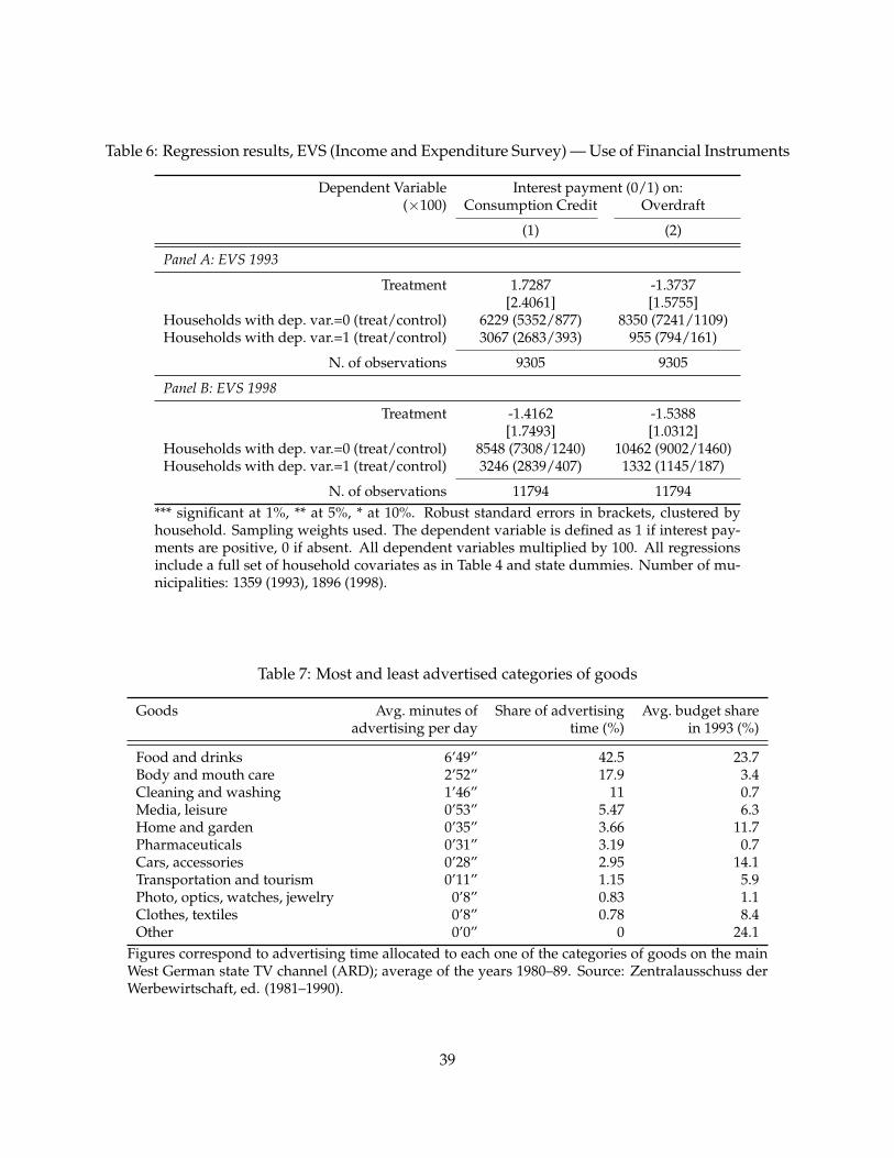
Table 6: Regression results, EVS (Income and Expenditure Survey) — Use of Financial Instruments

Dependent Variable Interest payment (0/1) on:(×100) Consumption Credit Overdraft

(1) (2)

Panel A: EVS 1993

Treatment 1.7287 -1.3737[2.4061] [1.5755]

Households with dep. var.=0 (treat/control) 6229 (5352/877) 8350 (7241/1109)Households with dep. var.=1 (treat/control) 3067 (2683/393) 955 (794/161)

N. of observations 9305 9305

Panel B: EVS 1998

Treatment -1.4162 -1.5388[1.7493] [1.0312]

Households with dep. var.=0 (treat/control) 8548 (7308/1240) 10462 (9002/1460)Households with dep. var.=1 (treat/control) 3246 (2839/407) 1332 (1145/187)

N. of observations 11794 11794*** significant at 1%, ** at 5%, * at 10%. Robust standard errors in brackets, clustered byhousehold. Sampling weights used. The dependent variable is defined as 1 if interest pay-ments are positive, 0 if absent. All dependent variables multiplied by 100. All regressionsinclude a full set of household covariates as in Table 4 and state dummies. Number of mu-nicipalities: 1359 (1993), 1896 (1998).

Table 7: Most and least advertised categories of goods

Goods Avg. minutes of Share of advertising Avg. budget shareadvertising per day time (%) in 1993 (%)

Food and drinks 6’49” 42.5 23.7Body and mouth care 2’52” 17.9 3.4Cleaning and washing 1’46” 11 0.7Media, leisure 0’53” 5.47 6.3Home and garden 0’35” 3.66 11.7Pharmaceuticals 0’31” 3.19 0.7Cars, accessories 0’28” 2.95 14.1Transportation and tourism 0’11” 1.15 5.9Photo, optics, watches, jewelry 0’8” 0.83 1.1Clothes, textiles 0’8” 0.78 8.4Other 0’0” 0 24.1

Figures correspond to advertising time allocated to each one of the categories of goods on the mainWest German state TV channel (ARD); average of the years 1980–89. Source: Zentralausschuss derWerbewirtschaft, ed. (1981–1990).

39

Table 8: Regression results, EVS (Income and Expenditure Survey) — Recomposition of consump-tion

Dependent variable: 100 × log(1+expenditures)

Treatment definition: Binary Continuous

(1) (2) (3) (4) (5)

Panel A: EVS 1993

Advertising 16.549*** 16.549*** 2.653*** 29.142*** 16.071***[0.388] [0.388] [0.062] [0.824] [0.495]

Treatment -8.96 -4.569 -8.96 -9.382 -14.267*[5.951] [2.899] [5.951] [5.802] [7.472]

Treatment × Advertising 1.537*** 1.537*** 0.246*** 1.979** 2.132***[0.547] [0.547] [0.088] [1.000] [0.714]

N. of observations 102355 102355 102355 102355 102355N. of households 9305 9305 9305 9305 9305

Panel B: EVS 1998

Advertising 3.398*** 3.398*** 0.545*** 21.637*** 3.518***[0.239] [0.239] [0.038] [0.759] [0.296]

Treatment 3.989 -1.068 3.989 -0.833 2.155[4.656] [1.607] [4.657] [3.254] [5.039]

Treatment × Advertising 0.197 0.197 0.032 1.234 0.059[0.284] [0.284] [0.046] [0.815] [0.355]


Household covariates N Y N N NAdvertising definition min p.d. min p.d. share min p.d. min p.d.

Regression weights S × B S × B S × B S S × B*** significant at 1%, ** at 5%, * at 10%. Robust standard errors in brackets, clusteredby municipality. Sampling weights used. Regressions are weighted either by the EVSsampling weights (S), or additionally also by the budget share of each category of con-sumption goods (S× B). The regression in column (3) uses the share of advertising time,rather than minutes of advertising per day, as explanatory variable (cf. Table 7). House-hold covariates included in column (2) are listed in Table 4. Number of municipalities:1359 (1993), 1896 (1998).

40

Table 9: Regression results, EVS — Recomposition of consumption: Robustness

Dependent Variable: 100 × log(1+expenditures)

Household Including “Treatment” threshold:clustering East Berlin -84.8dB -82.8dB -80.8dB

(1) (2) (3) (4) (5)

Panel A: EVS 1993

Advertising 16.549*** 16.549*** 16.605*** 16.532*** 16.663***[0.512] [0.388] [0.369] [0.349] [0.339]

Treatment -8.960* -10.559* -8.846 -10.664* -10.845**[5.327] [5.901] [5.718] [5.714] [5.526]

Treatment × Advertising 1.537*** 1.583*** 1.530*** 1.641*** 1.531***[0.571] [0.522] [0.544] [0.535] [0.537]


N. of households in treatment region 8035 9826 7752 7639 7404

Panel B: EVS 1998

Advertising 3.398*** 3.398*** 3.610*** 3.592*** 3.484***[0.355] [0.239] [0.257] [0.243] [0.249]

Treatment 3.989 3.808 3.197 2.486 1.189[3.593] [4.586] [4.208] [4.101] [4.020]

Treatment × Advertising 0.197 0.052 -0.049 -0.028 0.106[0.381] [0.305] [0.301] [0.291] [0.296]


N. of households in treatment region 10147 11259 9787 9598 9317

*** significant at 1%, ** at 5%, * at 10%. Robust standard errors in brackets, clustered by municipality(by household in column (1)). All regressions use the binary treatment definition and are weightedby EVS sampling weights and budget shares. Advertising defined as minutes per day (cf. Table 7).Number of municipalities: 1359 (1993), 1896 (1998).

41

Table 10: Regression results, EVS — Recomposition of consumption: Subsamples


Sample: -86.8dB -86.8dB -86.8dB±30dB ±20dB ±10dB

(1) (2) (3)

Panel A: EVS 1993

Advertising 16.699*** 16.596*** 16.870***[0.389] [0.390] [0.401]

Treatment -11.872** -10.164 5.496[6.045] [6.779] [7.814]

Treatment × Advertising 1.662*** 1.510** -0.326[0.584] [0.698] [0.791]

N. of observations 72842 53405 26081N. of households 6622 4855 2371

N. of municipalities 912 664 391

Panel B: EVS 1998

Advertising 3.565*** 3.434*** 3.112***[0.230] [0.222] [0.229]

Treatment 1.037 0.157 6.901[5.029] [5.171] [5.552]

Treatment × Advertising 0.368 0.646** 0.144[0.309] [0.328] [0.433]

N. of observations 87571 65626 34078N. of households 7961 5966 3098

N. of municipalities 1158 829 488*** significant at 1%, ** at 5%, * at 10%. Robust standard errorsin brackets, clustered by municipality. All regressions use thebinary treatment definition and are weighted by EVS samplingweights and budget shares. Advertising defined as minutes perday (cf. Table 7).

42

Table 11: Regression results, EVS — Recomposition: Robustness to Distance

Dependent Variable 100 × log(1+expenditures)

Whole Treatmentsample region

(1) (2)

Panel A: EVS 1993

Advertising 16.907*** 18.237***[1.388] [0.906]

Treatment -9.763 ·[7.718]

Treatment × Advertising 1.357* ·[0.762]

Distance -0.914 -1.702[7.364] [7.831]

Distance × Advertising -0.205 -0.173[0.765] [0.815]

N. of observations 102355 88385N. of households 9305 8035

N. of municipalities 1359 1194

Panel B: EVS 1998

Advertising 3.184*** 3.432***[0.576] [0.315]

Treatment 0.159 ·[5.582]

Treatment × Advertising 0.307 ·[0.385]

Distance -4.309 -4.928[3.240] [3.390]

Distance × Advertising 0.123 0.193[0.300] [0.313]

N. of observations 129734 111617N. of households 11794 10147

N. of municipalities 1896 1682*** significant at 1%, ** at 5%, * at 10%. Robust standarderrors in brackets, clustered by household. All regressionsuse the binary treatment definition and are weighted byEVS sampling weights and budget shares. Advertisingdefined as minutes per day (cf. Table 7). Distance to WestGermany measured in km.

43

A Supplemental Appendix: Additional tables (NOT FOR PUBLICA-TION)

A.1 Construction of the treatment indicator

Table A.1: West German Antennas (ARD)

Location Coordinates Altitude Height Power Frequency

Bungsberg, NDR-Mast 54◦13’0”N, 10◦43’8”E 136 154 260 703.25Neumunster 53◦58’46”N, 9◦50’59”E 27 141 500 527.25Hamburg-Moorfleet 53◦31’9”N, 10◦6’10”E 1 264 500 751.25Hamburg-Moorfleet 53◦31’9”N, 10◦6’10”E 1 264 100 203.25Dannenberg/Zernien 53◦3’56”N, 10◦53’50”E 102 234 250 647.25Scholzplatz, Berlin (West) 52◦30’22”N, 13◦13’10”E 66 220 100 189.25Tofhaus/Harz-West 51◦48’6”N, 10◦31’56”E 820 243 100 210.25Rimberg 50◦47’51”N, 9◦27’41”E 572 155 400 759.25Hoher Meißner 51◦13’42”N, 9◦51’50”E 705 155 100 189.25Kreuzberg (Rhon) 50◦22’12”N, 9◦58’48”E 927 182 100 55.25Ochsenkopf 50◦1’50”N, 11◦48’29”E 990 160 100 62.25Hoher Bogen 49◦14’57”N, 12◦53’27”E 976 70 500 743.25

Source: Norddeutscher Rundfunk, ed. (1989). Altitude and height of the antenna mast in meters.Power in kW. Frequency in MHz.

A.2 Definition of treatment area

Based on the antenna data above, we calculate average signal strength of the main West GermanTV broadcaster, ARD, in each one of the municipalities in East Germany (7529 municipalities in1993, 5793 municipalities in 1998). These data are then used to define the treatment region in theEVS (Income and Expenditure Survey): municipalities with an average signal strength higher than−86.8dB (the average level in Dresden) are defined as “treated”.

In other data sets observations may not be coded at the municipality level. Official data fromthe Statistical Yearbooks of the GDR is mostly available at the level of Bezirke (districts; 15 inEast Germany as of 1990). Figures 1 and 3 show the boundaries of these districts (a list of thedistricts can be found in Table A.2). The analysis in Table 1 is based on district-level data. Wedefine the districts of Dresden (south-east), Neubrandenburg and Rostock (north-east) as treated(cf. Figure 3).

Official migration statistics (as used in Tables 2 and A.3) are defined at the level of Kreise (coun-ties). In the years until 1994, there were 215 Kreise in East Germany. We consider a Kreis as treatedif average signal strength is higher than −86.8dB. This yields the following 23 Kreise in the con-trol area (listed in descending order of signal strength): Dresden Stadt, Altentreptow, Niesky,Anklam, Ribnitz-Damgarten, Malchin, Bautzen, Neubrandenburg Stadt, Ueckermunde, Teterow,Lobau, Pirna, Greifswald Land, Demmin, Gorlitz Land, Grimmen, Wolgast, Greifswald Stadt, Zit-tau, Gorlitz Stadt, Stralsund Land, Stralsund Stadt, Rugen.

44

The IAB’s census of plants (Establishment History Panel, BHP) used in Table 3 has a variableindicating in which Kreis each plant/establishment is located. However, the county borders usedin this context are the ones as of 2008. Due to several waves of county redistricting which oc-curred after 1994, there were only 86 Kreise left in East Germany as of 2008. Applying the samecriteria as above, we obtain the following list of 11 Kreise in the control region: Dresden Stadt,Neubrandenburg Stadt, Greifswald Stadt, Stralsund Stadt, Rugen, Demmin, Nordvorpommern,Ostvorpommern, Uecker-Randow, Gorlitz, Sachsische Schweiz-Osterzgebirge.

Table A.2: States and districts in East Germany

State (Bundesland) District (Bezirk)

Mecklenburg-Vorpommern Neubrandenburg*Rostock*Schwerin

Sachsen-Anhalt HalleMagdeburg

Brandenburg CottbusFrankfurt/OderPotsdam

Thuringen ErfurtGeraSuhl

Sachsen Dresden*Karl-Marx-Stadt (Chemnitz)Leipzig

Berlin Berlin (East)Districts were the administrative units of the GDR before1990, states are the administrative divisions of the FRG (EastGermany after 1990). The correspondence between districtsand states is only approximate. Asterisks (*) denote districtsin the control area (i.e., not covered by West German TV).

45

A.3 Migration data, 1991–1993

Table A.3 displays total migration rates between 1991 and 1993 from treatment and control areasand the breakdown of these rates by destination (Berlin, West Germany, control region, and treat-ment region). The numbers capture the moves of people that move out of their Kreis (district) ofresidence to another Kreis (they do not capture moves within the same Kreis).

The table suggests that total migration rates were low and similar in treatment and control ar-eas (considerably higher rates were recorded in the years 1989 and 1990; see Hunt, 2006. However,there is no breakdown of migration by place of origin available for those years, so that one cannotcompare migration rates by treatment region). The migration rates to areas outside of East Ger-many (i.e., Berlin and West Germany) were again similar when comparing control and treatmentregions. We observe that migration rates from control to treatment areas were higher than fromtreatment to control areas, since the treatment area is much larger than the control area (about 10%of the population in East Germany lived in the control area).

Table A.3: Migration matrix, 1991–1993

Origin Total by destination: Population

Berlin East Germany, East Germany, WestTreatment Control Germany

East Germany, 821,873 43,106 546,684 30,981 201,102 12,873,985Treatment (6.38%) (0.33%) (4.25%) (0.24%) (1.56%)East Germany, 100,934 4,141 32,421 36,640 27,732 1,634,665Control (6.17%) (0.25%) (1.98%) (2.24%) (1.7%)

Population figures refer to 1991. Figures in italics express the total number of people movingacross county borders from 1991 to 1993, relatively to original population size in 1991. Source:own analysis based on migration matrices (by Kreis), German Federal Statistical Office.

In Table A.4 we show how total outmigration rates from East Germany to West Germany dif-fered by treatment region and age category. Differential outmigration by age could be problematicif the response to “treatment” through West German media varies by age. The analysis belowshows, however, that outmigration rates were similar in treatment and control regions across allage categories.

46

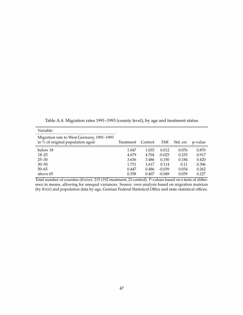
Table A.4: Migration rates 1991–1993 (county level), by age and treatment status

Variable:

Migration rate to West Germany, 1991–1993in % of original population aged: Treatment Control Diff. Std. err. p-value

below 18 1.047 1.035 0.012 0.076 0.87018–25 4.679 4.704 -0.025 0.235 0.91725–30 3.636 3.486 0.150 0.184 0.42030–50 1.731 1.617 0.114 0.11 0.30650–65 0.447 0.486 -0.039 0.034 0.262above 65 0.358 0.407 -0.049 0.039 0.227

Total number of counties (Kreise): 215 (192 treatment, 23 control). P-values based on t-tests of differ-ence in means, allowing for unequal variances. Source: own analysis based on migration matrices(by Kreis) and population data by age, German Federal Statistical Office and state statistical offices.

47

A.4 Differences in consumption levels and advertising

Table A.5 presents the data underlying Figures 5 and 6.

Table A.5: Differences in consumption levels and advertising: Raw data

Share of Avg.advertising budget

Goods Treatment Control Difference Std.err. time (%) share (%)

Panel A: EVS 1993

Food and drinks 8.826 8.812 0.014 0.031 42.5 23.7Body and mouth care 6.558 6.568 -0.010 0.067 17.89 3.4Cleaning and washing 4.774 4.754 0.020 0.097 11 0.7Media, leisure 7.248 7.345 -0.096 0.044 5.47 6.3Home and garden 7.645 7.636 0.008 0.065 3.66 11.7Pharmaceuticals 3.125 3.213 -0.088 0.131 3.19 0.7Cras, accessories 5.960 6.122 -0.162 0.182 2.95 14.1Transportation and tourism 6.347 6.717 -0.370 0.107 1.15 5.9Photo, optics, watches, and jewelry 4.165 4.112 0.053 0.127 0.83 1.1Clothes and textiles 7.505 7.601 -0.096 0.048 0.78 8.4All other 8.908 8.930 -0.022 0.022 0 24.1

Panel B: EVS 1998

Food and drinks 7.231 7.178 0.053 0.024 42.5 15.5Body and mouth care 4.953 4.935 0.017 0.049 17.89 2.3Cleaning and washing 3.532 3.430 0.103 0.060 11 0.6Media, leisure 6.082 6.117 -0.035 0.036 5.47 6.2Home and garden 5.940 5.896 0.043 0.059 3.66 9.4Pharmaceuticals 3.681 3.688 -0.007 0.072 3.19 0.9Cars, accessories 4.939 4.728 0.211 0.136 2.95 12.9Transportation and tourism 4.206 4.632 -0.426 0.092 1.15 6.3Photo, optics, watches, jewelry 3.254 3.313 -0.060 0.087 0.83 1.2Clothes, textiles 5.838 5.715 0.123 0.067 0.78 6.1Other 8.173 8.110 0.063 0.021 0 38.6

Figures correspond to the logarithm of average consumption expenditures of all households in the respectiveregions. Refer also to the notes to Figures 5 and 6 and Table 7.

48

A.5 Additional robustness checks

A.5.1 Clustering levels

Consumption patterns could be correlated even across households located in different, neighbor-ing municipalities. That is why our default level of clustering in the regressions (clustering at themunicipality level) could be missing some patterns of correlation in the error terms.

Unfortunately, due to confidentiality reasons we do not know the exact coordinates of the mu-nicipalities of the households in the dataset and thus we cannot group neighboring municipalitiestogether. As an alternative approach, we divide each of the five post-Reunification states (Lander)of East Germany into cells corresponding to 1, 3, 5 or 10 dB of signal strength. For example, in thelast case, we would divide Saxony into 9 cells corresponding to signal strengths of (−106.8;−96.8],(−96.8;−86.8], (−86.8;−76.8], (−76.8;−66.8] dB etc. Even though some households in the samecell may lie in disjoint regions, in most cases one cell would consist of adjacent municipalities.

This method results in a number of clusters varying between approximately 300 (1dB cells) and40 (10dB cells). Results in Table A.6 below, based on our baseline regression of Table 8, column1, show that the aggregation of households into larger clusters does not affect the precision ofour estimates. In all cases (with the possible exception of the case of 10dB cells) the number ofresulting clusters is safely above the threshold suggested by Cameron et al. (2008), allaying fearsof overrejection of null hypotheses.

A.5.2 Omitting selected categories of consumption goods

Another concern could be the role of single categories of goods in our analysis. As evident inFigures 5 and 6, some categories of goods are responsible for a large share of the advertisingtime (most notably, food and drinks, body and mouth care, and cleaning and washing products),whereas other categories have almost no advertising. In table A.7, we replicate the baseline regres-sion of Table 8, column 1, omitting each one of the categories of consumption goods: starting incolumn (1) with the goods with zero advertising and ending in column (11), which leaves out foodand drinks (columns are sorted in increasing intensity of advertising for the omitted category).

The results are reassuring: point estimates on the interaction term of interest (Treatment ×Advertising) are mostly unchanged in magnitude and significance. In column (11) we drop thecategory with the highest intensity of advertising (42.5% of advertising time) and with the second-largest budget share (15.46%), food and drinks. Even in this case, the magnitude of the pointestimate is preserved at 1.927 (compared to the baseline estimate of 1.537), even though the largerstandard error reduces the p-value to 0.32.

A.5.3 Use of the continuous treatment definition

Tables A.8 and A.9 replicate all the results of the main paper using, where applicable, the contin-uous treatment definition instead of the threshold-based one. This alternative definition confirmsall results of the analysis in both magnitude and significance.

49

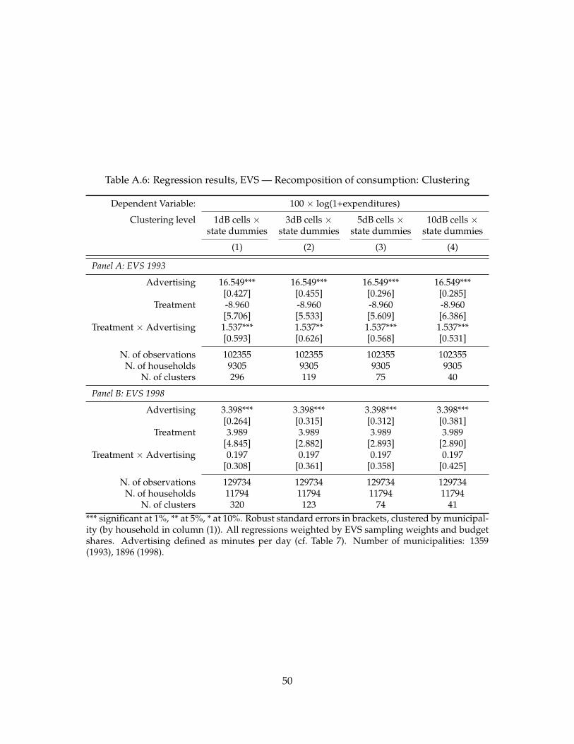
Table A.6: Regression results, EVS — Recomposition of consumption: Clustering


Clustering level 1dB cells × 3dB cells × 5dB cells × 10dB cells ×state dummies state dummies state dummies state dummies

(1) (2) (3) (4)

Panel A: EVS 1993

Advertising 16.549*** 16.549*** 16.549*** 16.549***[0.427] [0.455] [0.296] [0.285]

Treatment -8.960 -8.960 -8.960 -8.960[5.706] [5.533] [5.609] [6.386]

Treatment × Advertising 1.537*** 1.537** 1.537*** 1.537***[0.593] [0.626] [0.568] [0.531]

N. of observations 102355 102355 102355 102355N. of households 9305 9305 9305 9305

N. of clusters 296 119 75 40

Panel B: EVS 1998

Advertising 3.398*** 3.398*** 3.398*** 3.398***[0.264] [0.315] [0.312] [0.381]

Treatment 3.989 3.989 3.989 3.989[4.845] [2.882] [2.893] [2.890]

Treatment × Advertising 0.197 0.197 0.197 0.197[0.308] [0.361] [0.358] [0.425]

N. of observations 129734 129734 129734 129734N. of households 11794 11794 11794 11794

N. of clusters 320 123 74 41*** significant at 1%, ** at 5%, * at 10%. Robust standard errors in brackets, clustered by municipal-ity (by household in column (1)). All regressions weighted by EVS sampling weights and budgetshares. Advertising defined as minutes per day (cf. Table 7). Number of municipalities: 1359(1993), 1896 (1998).

50

Tabl

eA

.7:R

egre

ssio

nre

sult

s,EV

S—

Rec

ompo

siti

onof

cons

umpt

ion:

Om

itti

ngca

tego

ries

Dep

ende

ntV

aria

ble:

100×

log(

1+ex

pend

itur

es)

Om

itte

dca

tego

ry:

Oth

erC

loth

es,

Phot

o,Tr

ansp

.,C

ars

Phar

ma-

Hom

e,M

edia

,C

lean

ing,

Body

Food

,(n

oad

v.)

text

iles

opti

csto

uris

mce

utic

als

gard

enle

isur

ew

ashi

ngca

redr

inks

(1)

(2)

(3)

(4)

(5)

(6)

(7)

(8)

(9)

(10)

(11)

Pane

lA:E

VS

1993

Adv

erti

sing

30.2

61**

*16

.749

***

15.6

63**

*15

.371

***

11.7

80**

*15

.993

***

16.6

62**

*16

.273

***

16.4

98**

*17

.138

***

-85.

601*

**[0

.649

][0

.401

][0

.383

][0

.403

][0

.696

][0

.388

][0

.381

][0

.401

][0

.389

][0

.392

][1

.669

]Tr

eatm

ent

-12.

759

-8.8

45-9

.187

-6.3

45-7

.083

*-8

.954

-10.

588*

-8.7

87-9

.023

-9.0

55-9

.104

[8.2

74]

[6.3

88]

[5.9

47]

[6.7

82]

[3.9

05]

[6.0

18]

[6.3

68]

[6.2

60]

[5.9

68]

[6.0

79]

[5.8

28]

Trea

tmen

t×A

dver

tisi

ng2.

182*

*1.

518*

**1.

573*

**1.

122*

*1.

275*

1.53

6***

1.75

1***

1.51

8***

1.53

8***

1.52

2***

1.92

7[0

.909

][0

.580

][0

.545

][0

.566

][0

.762

][0

.548

][0

.564

][0

.565

][0

.548

][0

.546

][1

.936

]

N.o

fobs

erva

tion

s93

050

9305

093

050

9305

093

050

9305

093

050

9305

093

050

9305

093

050

N.o

fhou

seho

lds

9305

9305

9305

9305

9305

9305

9305

9305

9305

9305

9305

Pane

lB:E

VS

1998

Adv

erti

sing

30.7

62**

*2.

191*

**2.

556*

**0.

722

-0.8

013.

018*

**2.

434*

**3.

138*

**3.

549*

**4.

500*

**-1

51.2

11**

*[0

.451

][0

.258

][0

.235

][0

.441

][0

.568

][0

.238

][0

.249

][0

.235

][0

.239

][0

.260

][1

.612

]Tr

eatm

ent

1.62

33.

295

4.14

68.

026

0.91

44.

042

3.96

24.

553

3.95

64.

031

3.99

4Tr

eatm

ent×

Adv

erti

sing

[5.2

83]

[4.5

30]

[4.7

75]

[7.5

56]

[2.1

82]

[4.6

95]

[4.6

42]

[4.9

37]

[4.6

68]

[4.7

36]

[4.4

04]

0.61

50.

311

0.17

1-0

.439

0.57

90.

191

0.2

0.15

70.

194

0.21

50.

18[0

.526

][0

.302

][0

.280

][0

.481

][0

.610

][0

.283

][0

.296

][0

.280

][0

.284

][0

.301

][1

.825

]

N.o

fobs

erva

tion

s11

7940

1179

4011

7940

1179

4011

7940

1179

4011

7940

1179

4011

7940

1179

4011

7940

N.o

fhou

seho

lds

1179

411

794

1179

411

794

1179

411

794

1179

411

794

1179

411

794

1179

4**

*si

gnifi

cant

at1%

,**

at5%

,*at

10%

.R

obus

tsta

ndar

der

rors

inbr

acke

ts,c

lust

ered

bym

unic

ipal

ity

(by

hous

ehol

din

colu

mn

(1))

.A

llre

gres

sion

sw

eigh

ted

byEV

Ssa

mpl

ing

wei

ghts

and

budg

etsh

ares

.Adv

erti

sing

defin

edas

min

utes

per

day

(cf.

Tabl

e7)

.Num

ber

ofm

unic

ipal

itie

s:13

59(1

993)

,189

6(1

998)

.

51

Tabl

eA

.8:R

egre

ssio

nre

sult

s,EV

S—

Agg

rega

teco

nsum

ptio

nbe

havi

oran

dfin

anci

alin

stru

men

ts:C

onti

nuou

str

eatm

entd

efini

tion

Dep

ende

ntV

aria

ble

log

Dis

posa

ble

log

Tota

lPri

vate

Savi

ngs>

0In

tere

stpa

ymen

t(0/

1)on

:(×

100)

Inco

me

Con

sum

ptio

n(0

/1)

Con

sum

ptio

nC

redi

tO

verd

raft

Equi

vale

ntto

:Ta

ble

5,Ta

ble

5,Ta

ble

5,Ta

ble

6,Ta

ble

6,co

lum

n(1

)co

lum

n(2

)co

lum

n(3

)co

lum

n(1

)co

lum

n(2

)

(1)

(2)

(3)

(4)

(5)

Pane

lA:E

VS

1993

Trea

tmen

t(co

ntin

uous

)-0

.626

0.44

4-0

.623

2.63

8-0

.789

[2.3

26]

[1.6

05]

[2.5

93]

[2.9

06]

[1.8

75]

N.o

fobs

erva

tion

s93

0593

0593

0593

0593

05

Pane

lB:E

VS

1998

Trea

tmen

t(co

ntin

uous

)-1

.092

-0.1

470.

047

-0.6

67-0

.899

[2.1

68]

[1.4

93]

[1.7

98]

[1.8

94]

[1.2

39]

N.o

fobs

erva

tion

s11

794

1179

411

794

1179

411

794

***

sign

ifica

ntat

1%,*

*at

5%,*

at10

%.

Rob

ust

stan

dard

erro

rsin

brac

kets

,clu

ster

edby

mun

icip

alit

y.Sa

mpl

ing

wei

ghts

used

.A

llde

pend

entv

aria

bles

mul

tipl

ied

by10

0.A

llre

gres

sion

sin

clud

ea

full

seto

fst

ate

dum

mie

san

dho

useh

old

cova

riat

esas

inTa

ble

4,ex

cept

colu

mn

(1),

whe

relo

gdi

spos

able

inco

me

isex

clud

edfr

omth

ese

tof

regr

esso

rs.C

olum

n(3

)cor

resp

onds

toa

linea

rpr

obab

ility

mod

el.T

hede

pend

entv

aria

ble

isde

fined

as1

ifsa

ving

sar

epo

siti

ve,

0ot

herw

ise.

Col

umns

(4)

and

(5):

the

depe

nden

tva

riab

leis

defin

edas

1if

inte

rest

paym

ents

are

posi

tive

,0if

abse

nt.N

umbe

rof

mun

icip

alit

ies:

1359

(199

3),1

896

(199

8).

52

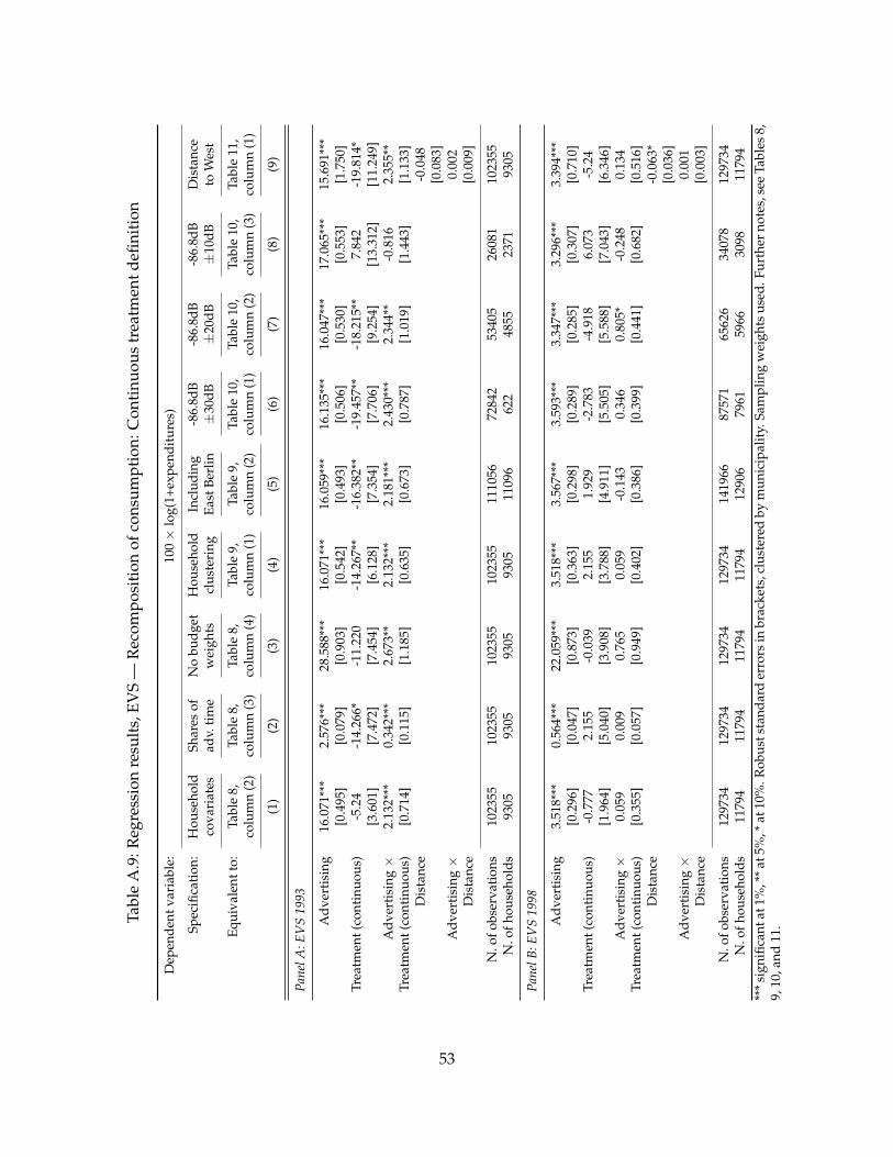
Tabl

eA

.9:R

egre

ssio

nre

sult

s,EV

S—

Rec

ompo

siti

onof

cons

umpt

ion:

Con

tinu

ous

trea

tmen

tdefi

niti

on

Dep

ende

ntva

riab

le:

100×

log(

1+ex

pend

itur

es)

Spec

ifica

tion

:H

ouse

hold

Shar

esof

No

budg

etH

ouse

hold

Incl

udin

g-8

6.8d

B-8

6.8d

B-8

6.8d

BD

ista

nce

cova

riat

esad

v.ti

me

wei

ghts

clus

teri

ngEa

stBe

rlin

±30

dB±

20dB

±10

dBto

Wes

t

Equi

vale

ntto

:Ta

ble

8,Ta

ble

8,Ta

ble

8,Ta

ble

9,Ta

ble

9,Ta

ble

10,

Tabl

e10

,Ta

ble

10,

Tabl

e11

,co

lum

n(2

)co

lum

n(3

)co

lum

n(4

)co

lum

n(1

)co

lum

n(2

)co

lum

n(1

)co

lum

n(2

)co

lum

n(3

)co

lum

n(1

)

(1)

(2)

(3)

(4)

(5)

(6)

(7)

(8)

(9)

Pane

lA:E

VS

1993

Adv

erti

sing

16.0

71**

*2.

576*

**28

.588

***

16.0

71**

*16

.059

***

16.1

35**

*16

.047

***

17.0

65**

*15

.691

***

[0.4

95]

[0.0

79]

[0.9

03]

[0.5

42]

[0.4

93]

[0.5

06]

[0.5

30]

[0.5

53]

[1.7

50]

Trea

tmen

t(co

ntin

uous

)-5

.24

-14.

266*

-11.

220

-14.

267*

*-1

6.38

2**

-19.

457*

*-1

8.21

5**

7.84

2-1

9.81

4*[3

.601

][7

.472

][7

.454

][6

.128

][7

.354

][7

.706

][9

.254

][1

3.31

2][1

1.24

9]A

dver

tisi

ng×

2.13

2***

0.34

2***

2.67

3**

2.13

2***

2.18

1***

2.43

0***

2.34

4**

-0.8

162.

355*

*Tr

eatm

ent(

cont

inuo

us)

[0.7

14]

[0.1

15]

[1.1

85]

[0.6

35]

[0.6

73]

[0.7

87]

[1.0

19]

[1.4

43]

[1.1

33]

Dis

tanc

e-0

.048

[0.0

83]

Adv

erti

sing×

0.00

2D

ista

nce

[0.0

09]

N.o

fobs

erva

tion

s10

2355

1023

5510

2355

1023

5511

1056

7284

253

405

2608

110

2355

N.o

fhou

seho

lds

9305

9305

9305

9305

1109

662

248

5523

7193

05

Pane

lB:E

VS

1998

Adv

erti

sing

3.51

8***

0.56

4***

22.0

59**

*3.

518*

**3.

567*

**3.

593*

**3.

347*

**3.

296*

**3.

394*

**[0

.296

][0

.047

][0

.873

][0

.363

][0

.298

][0

.289

][0

.285

][0

.307

][0

.710

]Tr

eatm

ent(

cont

inuo

us)

-0.7

772.

155

-0.0

392.

155

1.92

9-2

.783

-4.9

186.

073

-5.2

4[1

.964

][5

.040

][3

.908

][3

.788

][4

.911

][5

.505

][5

.588

][7

.043

][6

.346

]A

dver

tisi

ng×

0.05

90.

009

0.76

50.

059

-0.1

430.

346

0.80

5*-0

.248

0.13

4Tr

eatm

ent(

cont

inuo

us)

[0.3

55]

[0.0

57]

[0.9

49]

[0.4

02]

[0.3

86]

[0.3

99]

[0.4

41]

[0.6

82]

[0.5

16]

Dis

tanc

e-0

.063

*[0

.036

]A

dver

tisi

ng×

0.00

1D

ista

nce

[0.0

03]

N.o

fobs

erva

tion

s12

9734

1297

3412

9734

1297

3414

1966

8757

165

626

3407

812

9734

N.o

fhou

seho

lds

1179

411

794

1179

411

794

1290

679

6159

6630

9811

794

***s

igni

fican

tat1

%,*

*at5

%,*

at10

%.R

obus

tsta

ndar

der

rors

inbr

acke

ts,c

lust

ered

bym

unic

ipal

ity.

Sam

plin

gw

eigh

tsus

ed.F

urth

erno

tes,

see

Tabl

es8,

9,10

,and

11.

53

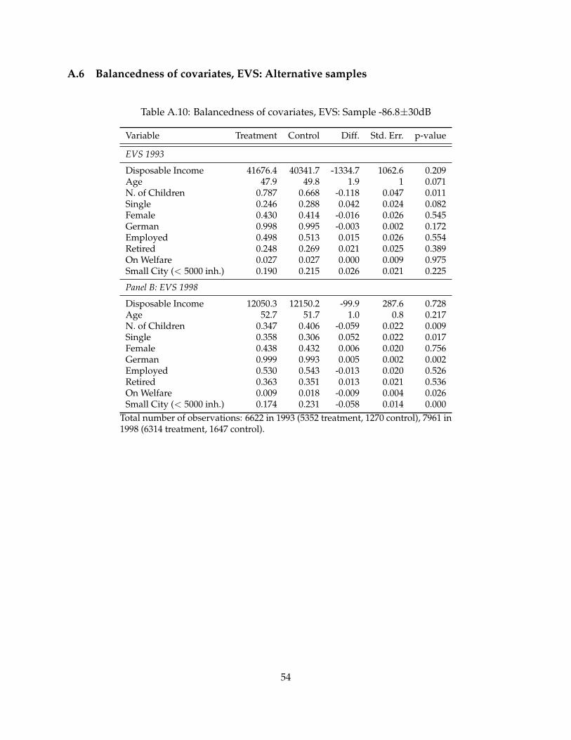
A.6 Balancedness of covariates, EVS: Alternative samples

Table A.10: Balancedness of covariates, EVS: Sample -86.8±30dB


EVS 1993

Disposable Income 41676.4 40341.7 -1334.7 1062.6 0.209Age 47.9 49.8 1.9 1 0.071N. of Children 0.787 0.668 -0.118 0.047 0.011Single 0.246 0.288 0.042 0.024 0.082Female 0.430 0.414 -0.016 0.026 0.545German 0.998 0.995 -0.003 0.002 0.172Employed 0.498 0.513 0.015 0.026 0.554Retired 0.248 0.269 0.021 0.025 0.389On Welfare 0.027 0.027 0.000 0.009 0.975Small City (< 5000 inh.) 0.190 0.215 0.026 0.021 0.225

Panel B: EVS 1998

Disposable Income 12050.3 12150.2 -99.9 287.6 0.728Age 52.7 51.7 1.0 0.8 0.217N. of Children 0.347 0.406 -0.059 0.022 0.009Single 0.358 0.306 0.052 0.022 0.017Female 0.438 0.432 0.006 0.020 0.756German 0.999 0.993 0.005 0.002 0.002Employed 0.530 0.543 -0.013 0.020 0.526Retired 0.363 0.351 0.013 0.021 0.536On Welfare 0.009 0.018 -0.009 0.004 0.026Small City (< 5000 inh.) 0.174 0.231 -0.058 0.014 0.000

Total number of observations: 6622 in 1993 (5352 treatment, 1270 control), 7961 in1998 (6314 treatment, 1647 control).

54

Table A.11: Balancedness of covariates, EVS: Sample −86.8± 20dB


Panel A: EVS 1993

Disposable Income 40821.8 41747.6 -925.8 1122.1 0.409Age 49.4 48 1.4 1.1 0.191N. of Children 0.691 0.780 -0.089 0.049 0.067Single 0.275 0.248 0.027 0.026 0.299Female 0.401 0.431 -0.030 0.027 0.276German 0.995 0.998 -0.004 0.003 0.218Employed 0.534 0.501 0.033 0.028 0.232Retired 0.251 0.250 0.001 0.026 0.984On Welfare 0.025 0.028 -0.003 0.009 0.773Small City (< 5000 inh.) 0.228 0.192 0.037 0.022 0.103

Panel B: EVS 1998

Disposable Income 48627 48313.8 313.2 1204.3 0.795Age 51.4 52.7 -1.3 1.3 0.113N. of Children 0.422 0.346 0.076 0.059 0.001Single 0.296 0.359 -0.064 0.032 0.005Female 0.433 0.439 -0.006 0.034 0.777German 0.990 0.999 -0.008 0.002 0.000Employed 0.553 0.530 0.023 0.034 0.278Retired 0.338 0.363 -0.024 0.034 0.262On Welfare 0.017 0.009 0.008 0.010 0.052Small City (< 5000 inh.) 0.236 0.176 0.060 0.029 0.000

Total number of observations: 4855 in 1993 (3597 treatment, 1258 control), 5966in 1998 (4331 treatment, 1635 control).

55

Table A.12: Balancedness of covariates, EVS: Sample −86.8± 10dB


Panel A: EVS 1993

Disposable Income 42974.5 41764 1210.5 1380.8 0.381Age 49.4 47.8 1.6 1.3 0.227N. of Children 0.754 0.782 -0.028 0.059 0.637Single 0.229 0.249 -0.020 0.032 0.537Female 0.369 0.434 -0.065 0.034 0.052German 0.997 0.998 -0.001 0.002 0.547Employed 0.561 0.502 0.059 0.034 0.083Retired 0.265 0.248 0.017 0.034 0.614On Welfare 0.014 0.027 -0.013 0.010 0.165Small City (< 5000 inh.) 0.315 0.190 0.126 0.029 0.000

Panel B: EVS 1998

Disposable Income 51056.8 48249.6 2807.1 1497.9 0.061Age 51.6 52.6 -1.0 1.3 0.357N. of Children 0.433 0.347 0.086 0.059 0.005Single 0.283 0.360 -0.077 0.032 0.007Female 0.419 0.438 -0.018 0.034 0.483German 0.998 0.999 0 0.002 0.850Employed 0.570 0.532 0.037 0.034 0.157Retired 0.343 0.358 -0.015 0.034 0.582On Welfare 0.006 0.009 -0.003 0.010 0.412Small City (< 5000 inh.) 0.319 0.172 0.147 0.029 0.000

Total number of observations: 2371 in 1993 (1216 treatment, 1155 control), 3098in 1998 (1518 treatment, 1580 control).

56

a tear in the iron curtain: the impact of western ... · a tear in the iron curtain: the impact of...

Documents