a taylor method for numerical solution of generalized pantograph equations with linear functional...

Journal of Computational and Applied Mathematics 200 (2007) 217–225www.elsevier.com/locate/cam

A Taylor method for numerical solution of generalized pantographequations with linear functional argument

Mehmet Sezera, Aysegül Akyüz-Dascıoglub,∗aDepartment of Mathematics, Faculty of Science, Mugla University, Mugla, Turkey

bDepartment of Mathematics, Faculty of Science, Pamukkale University, Denizli, Turkey

Received 16 June 2005; received in revised form 18 December 2005

Abstract

This paper is concerned with a generalization of a functional differential equation known as the pantograph equation whichcontains a linear functional argument. In this paper, we introduce a numerical method based on the Taylor polynomials for theapproximate solution of the pantograph equation with retarded case or advanced case. The method is illustrated by studying theinitial value problems. The results obtained are compared by the known results.© 2006 Elsevier B.V. All rights reserved.

MSC: 34K06; 34K28

Keywords: Pantograph equations; Functional equations; Taylor method

1. Introduction

Taylor methods have been given to solve linear differential, integral and integro-differential equations with approx-imate and exact solutions [15,18,21,24]. In recent years, many papers have been devoted to problem of approximatesolution of difference, differential-difference and integro-difference equations [10–12,22]. Our purpose in this study isto develop and to apply mentioned methods to the generalized pantograph equation

y(m)(t) =J∑

j=0

m−1∑k=0

Pjk(t)y(k)(�j t + �j ) + f (t) (1)

which is a generalization of the pantograph equations given in [4,8,16,17] with the initial conditions

m−1∑k=0

ciky(k)(0) = �i , i = 0, 1, . . . , m − 1 (2)

∗ Corresponding author.E-mail addresses: [email protected] (M. Sezer), [email protected] (A. Akyüz-Dascıoglu).

0377-0427/$ - see front matter © 2006 Elsevier B.V. All rights reserved.doi:10.1016/j.cam.2005.12.015

http://www.elsevier.com/locate/cam

mailto:[email protected]

mailto:[email protected]

218 M. Sezer, A. Akyüz-Dascıoglu / Journal of Computational and Applied Mathematics 200 (2007) 217–225

and to find the solution in terms of the Taylor polynomial form, in the origin,

y(t) =N∑

n=0

yntn, yn = y(n)(0)

n! . (3)

Here Pjk(t) and f (t) are analytical functions; cik , �i , �j and �j are real or complex constants; the coefficients yn,n = 0, 1, . . . , N are Taylor coefficients to be determined.

In recent years, there has been a growing interest in the numerical treatment of pantograph equations of the retardedand advanced type.A special feature of this type is the existence of compactly supported solutions [4]. This phenomenonwas studied in [3] and has direct applications to approximation theory and to wavelets [5].

Pantograph equations are characterized by the presence of a linear functional argument and play an important role inexplaining many different phenomena. In particular they turn out to be fundamental when ODEs-based model fail. Theseequations arise in industrial applications [9,19] and in studies based on biology, economy, control and electrodynamics[1,2].

2. Fundamental relations

Let us convert expressions defined in (1)–(3) to the matrix forms. Let us first assume that the functions y(t) and itsderivative y(k)(t) can be expanded to Taylor series about t = 0 in the form

y(k)(t) =∞∑

n=0

y(k)n tn, (4)

where for k = 0, y(0)(t) = y(t) and y(0)n = yn.

Now, let us differentiate expression (4) with respect to t and then put n → n + 1

y(k+1)(t) =∞∑

n=1

ny(k)n tn−1 =

∞∑n=0

(n + 1)y(k)n+1t

n. (5)

It is clear, from (4), that

y(k+1)(t) =∞∑

n=0

y(k+1)n tn. (6)

Using relations (5) and (6), we have the recurrence relation between the Taylor coefficients of y(k)(t) and y(k+1)(t)

y(k+1)n = (n + 1)y

(k)n+1, n, k = 0, 1, 2, . . . . (7)

If we take n = 0, 1, . . . , N and assume y(k)n = 0 for n > N , then we can transform system (7) into the matrix form

Y(k+1) = MY(k), k = 0, 1, 2, . . . , (8)

where

Y(k) =

⎡⎢⎢⎢⎣

y(k)0

y(k)1...

y(k)N

⎤⎥⎥⎥⎦ , M =

⎡⎢⎢⎢⎢⎣

0 1 0 · · · 00 0 2 · · · 0...

......

. . ....

0 0 0 · · · N

0 0 0 · · · 0

⎤⎥⎥⎥⎥⎦ .

For k = 0, 1, 2, . . ., it follows from relation (8) that

Y(k) = MkY, (9)

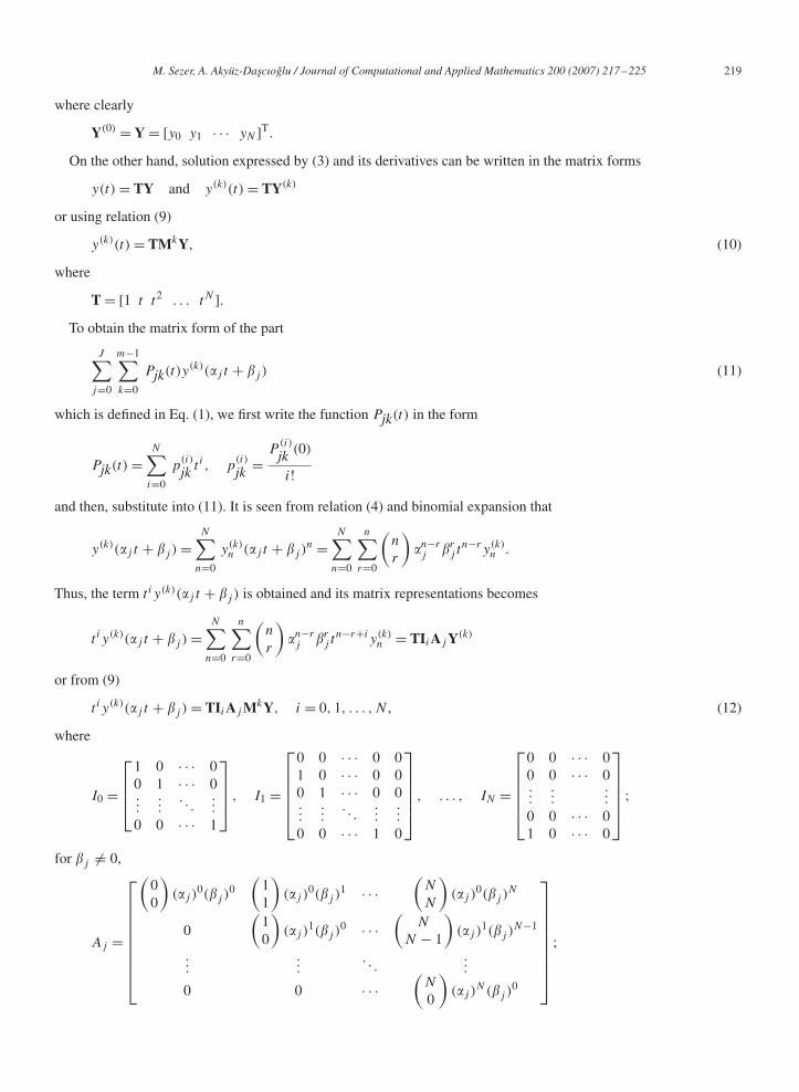
M. Sezer, A. Akyüz-Dascıoglu / Journal of Computational and Applied Mathematics 200 (2007) 217–225 219

where clearly

Y(0) = Y = [y0 y1 · · · yN ]T.

On the other hand, solution expressed by (3) and its derivatives can be written in the matrix forms

y(t) = TY and y(k)(t) = TY(k)

or using relation (9)

y(k)(t) = TMkY, (10)

where

T = [1 t t2 . . . tN ].To obtain the matrix form of the part

J∑j=0

m−1∑k=0

Pjk(t)y(k)(�j t + �j ) (11)

which is defined in Eq. (1), we first write the function Pjk(t) in the form

Pjk(t) =N∑

i=0

p(i)

jk t i , p(i)

jk =P

(i)

jk (0)

i!and then, substitute into (11). It is seen from relation (4) and binomial expansion that

y(k)(�j t + �j ) =N∑

n=0

y(k)n (�j t + �j )

n =N∑

n=0

n∑r=0

(n

r

)�n−rj �r

j tn−ry(k)

n .

Thus, the term t iy(k)(�j t + �j ) is obtained and its matrix representations becomes

t iy(k)(�j t + �j ) =N∑

n=0

n∑r=0

(n

r

)�n−rj �r

j tn−r+iy(k)

n = TIiAj Y(k)

or from (9)

t iy(k)(�j t + �j ) = TIiAj MkY, i = 0, 1, . . . , N , (12)

where

I0 =

⎡⎢⎢⎣

1 0 · · · 00 1 · · · 0...

.... . .

...

0 0 · · · 1

⎤⎥⎥⎦ , I1 =

⎡⎢⎢⎢⎢⎣

0 0 · · · 0 01 0 · · · 0 00 1 · · · 0 0...

.... . .

......

0 0 · · · 1 0

⎤⎥⎥⎥⎥⎦ , . . . , IN =

⎡⎢⎢⎢⎢⎣

0 0 · · · 00 0 · · · 0...

......

0 0 · · · 01 0 · · · 0

⎤⎥⎥⎥⎥⎦ ;

for �j �= 0,

Aj =

⎡⎢⎢⎢⎢⎢⎢⎢⎢⎣

(00

)(�j )

0(�j )0

(11

)(�j )

0(�j )1 · · ·

(N

N

)(�j )

0(�j )N

0

(10

)(�j )

1(�j )0 · · ·

(N

N − 1

)(�j )

1(�j )N−1

......

. . ....

0 0 · · ·(

N

0

)(�j )

N (�j )0

⎤⎥⎥⎥⎥⎥⎥⎥⎥⎦

;


and for �j = 0,

Aj =

⎡⎢⎢⎣

(�j )0 0 · · · 0

0 (�j )1 · · · 0

......

. . ....

0 0 · · · (�j )N

⎤⎥⎥⎦ .

Utilizing expression (12), we obtain the matrix form of the part (11) as

J∑j=0

m−1∑k=0

N∑i=0

p(i)

jk TIiAj MkY. (13)

We now assume that the function f (t) can be expanded as

f (t) =N∑

n=0

fntn, fn = f (n)(0)

n!or written in the matrix form

f (t) = TF, (14)

where F = [f0 f1 . . . fN ]T.Next, by means of relation (10), we can obtain the corresponding matrix form for the initial conditions (2) as

m−1∑k=0

cikT(0)MkY = �i , i = 0, 1, . . . , m − 1, (15)

where

T(0) = [1 0 0 · · · 0].

3. Method of solution

We are now ready to construct the fundamental matrix equation corresponding to Eq. (1). For this purpose, substitutingmatrix relations (10), (13) and (14) into Eq. (1) and then simplifying, we obtain the fundamental matrix equation⎧⎨

⎩Mm −J∑

j=0

m−1∑k=0

N∑i=0

p(i)

jk IiAj Mk

⎫⎬⎭Y = F (16)

which corresponds to a system of (N + 1) algebraic equations for the (N + 1) unknown coefficients y0, y1, . . . , yN .Briefly, we can write Eq. (16) in the form

WY = F or [W; F],where

W = [wnh], n, h = 0, 1, . . . , N .

Also, the matrix form (15) for conditions (2) can be written as

UiY = �i or [Ui; �i], i = 0, 1, . . . , m − 1,

where

Ui =m−1∑k=0

cikT(0)Mk = [ui0 ui1 · · · uiN ].


To obtain solution of Eq. (1) under conditions (2), by replacing the m rows matrices [Ui; �i] by the last m rows ofthe matrix [W; F], we have the augmented matrix

[W; F] =

⎡⎢⎢⎢⎢⎢⎢⎢⎢⎢⎢⎢⎣

w00 w01 . . . w0N ; f0w10 w11 . . . w1N ; f1...

......

......

wN−m,0 wN−m,1 . . . wN−m,N ; fN−m

u00 u01 . . . u0N ; �0u10 u11 . . . u1N ; �1...

......

......

um−1,0 um−1,1 . . . um−1,N ; �m−1

⎤⎥⎥⎥⎥⎥⎥⎥⎥⎥⎥⎥⎦

.

If det W �= 0, then we can write

Y = (W)−1F.

Thus the coefficients yn, n = 0, 1, . . . , N are uniquely determined by this equation.We can easily check the accuracy of the solutions as follows. Since the obtained polynomial solution is an approximate

solution of Eq. (1), it must be satisfied approximately; that is, for t = tr , r = 0, 1, . . .

E(tr ) =∣∣∣∣∣∣y(m)(tr ) −

J∑j=0

m−1∑k=0

Pjk(tr )y(k)(�j tr + �j ) − f (tr )

∣∣∣∣∣∣�0 (17)

or E(tr )�10−kr (kr any positive integer) is prescribed, then the truncation limit N is increased until the differenceE(tr ) at each of the points tr becomes smaller than the prescribed 10−k .

4. Illustrative examples

In this section, several numerical examples are given to illustrate the properties of the method and all of them wereperformed on the computer using a program written in Mathcad 2001 Professional. The absolute errors in Tables 2–4are the values of |y(x) − yN(x)| at selected points.

Example 1. Consider the linear delay differential equation of first order

y′(t) = −y(0.8t) − y(t), y(0) = 1. (18)

From Eq. (16), the fundamental matrix equation of the problem is

(M + I0 + A1)Y = F,

where I0 is unit matrix, M and A1 for �1 = 0.8, �1 = 0 are defined in relations (8) and (12), respectively.

Table 1 shows solutions of Eq. (18) with N = 8, 11 and 19 by presented method. The previous results of Rao andPalanisamy by Walsh series approach [20], Hwang by delayed unit step function (DUSF) series approach [13], andHwang and Shih by Laguerre series approach [14] are also given in Table 1 for comparison. The Taylor method seemsmore rapidly convergent than Laguerre series, and with errors more under control than for the Walsh or DUSF series.

Example 2. Consider the following problem:

y′(t) = 1

2et/2y

(t

2

)+ 1

2y(t), y(0) = 1, 0� t �1 (19)

which has the exact solution y(t) = et .


Table 1Comparison of the solutions of Eq. (18)

t Walsh series DUSF series Laguerre series Taylor series methodmethod method method

m = 100, h = 0.01 n = 20 n = 30 N = 8 N = 11 N = 19, y(t) N = 19, E(t)

0 1.000000 1.000000 0.999971 1.000000 1.000000 1.000000 1.000000000000000 8.44 E − 150.2 0.665621 0.664677 0.664703 0.664691 0.664691 0.664691 0.664691000828909 1.38 E − 140.4 0.432426 0.433540 0.433555 0.433561 0.433561 0.433561 0.433560778776339 3.22 E − 140.6 0.275140 0.276460 0.276471 0.276482 0.276483 0.276482 0.276482330222267 1.25 E − 140.8 0.170320 0.171464 0.171482 0.171484 0.171494 0.171484 0.171484111976062 7.38 E − 151 0.100856 0.102652 0.102679 0.102670 0.102744 0.102670 0.102670126574418 1.55 E − 14

Table 2Comparison of the absolute errors for Eq. (19)

t Spline method, h = 0.001 Adomian method Present methodwith 13 terms [8]

m = 2 [6] m = 3 [23] m = 4 [7] N = 8 N = 12 N = 15 N = 16

0.2 0.198 E − 7 1.37 E − 11 3.10 E − 15 0.00 1.440 E − 12 2.220 E − 16 2.220 E − 16 2.22 E − 160.4 0.473 E − 7 3.27 E − 11 7.54 E − 15 2.22 E − 16 7.524 E − 10 1.332 E − 15 2.220 E − 16 2.22 E − 160.6 0.847 E − 7 5.86 E − 11 1.39 E − 14 2.22 E − 16 2.953 E − 8 2.189 E − 13 2.220 E − 16 2.22 E − 160.8 0.135 E − 6 9.54 E − 11 2.13 E − 14 1.33 E − 15 4.018 E − 7 9.361 E − 12 1.332 E − 15 0.001 0.201 E − 6 1.43 E − 10 3.19 E − 14 4.88 E − 15 3.059 E − 6 1.729 E − 10 5.018 E − 14 2.22 E − 15

When the presented method is applying to Eq. (19), the fundamental matrix equation becomes(M − 1

2I0 −

N∑i=0

p(i)IiA1

)Y = F,

where p(i) is the Taylor coefficients of 1/2et/2, A1 for �1 = 0.5, �1 = 0 and Ii are defined in relation (12). Hence, thecomputed results are compared with other methods [6–8,23] in Table 2. The Taylor method has better results than thespline methods for different N . However, the absolute errors of Adomian and the Taylor methods seem like each other.

Example 3. Consider the pantograph equation of first order

y′(t) = −y(t) + q

2y(qt) − q

2e−qt , y(0) = 1, (20)

where y(t)= e−t . Table 3 compares the results of the present method and the collocation method [17] for this problem.Note that q = 1 is not a pantograph equation, is a linear differential equation. In any case, the Taylor method has farbetter results than collocation method.

Example 4. Consider the pantograph equation with variable coefficients

y′(t) = −y(t) + �1(t)y(t/2) + �2(t)y(t/4), y(0) = 1.

Here �1(t) = −e−0.5t sin(0.5t), �2(t) = −2e−0.75t cos(0.5t) sin(0.25t). It can be seen that the exact solution of thisproblem is y(t) = e−t cos(t) [16]. Using the method with N = 7, we obtain the approximate solution

y(t) = 1 − t + 1

3t3 − 1

6t4 + 3333333333333

99999999999991t5 − 6105006105

3846153846149t7.

Note that the coefficients y0, y1, y2, y3, y4, y6 are the same as the exact solution and others are the same till the 15decimal place.


Table 3Comparison of the absolute errors for Eq. (20)

t q = 1 q = 0.2

Collocation M. Present method Collocation M. Present method

m = 2 N = 6 N = 13 m = 2 N = 6 N = 13

2−1 5.005 E − 06 1.458 E − 06 7.772 E − 16 2.719 E − 05 1.458 E − 06 7.772 E − 162−2 1.877 E − 07 1.174 E − 08 1.110 E − 16 1.080 E − 06 1.174 E − 08 1.110 E − 162−3 6.434 E − 09 9.315 E − 11 2.220 E − 16 3.817 E − 08 9.315 E − 11 2.220 E − 162−4 2.106 E − 10 7.334 E − 13 0.000 1.269 E − 09 7.334 E − 13 0.0002−5 6.700 E − 12 5.662 E − 15 1.110 E − 16 4.090 E − 11 5.662 E − 15 1.110 E − 162−6 2.100 E − 13 0.000 0.000 1.200 E − 12 0.000 0.000

Example 5 (Evans and Raslan, [8]). Consider the pantograph equation of second order

y′′(t) = 3

4y(t) + y

(t

2

)− t2 + 2, y(0) = 0, y′(0) = 0, 0� t �1.

The fundamental matrix equation of this problem is

(M2 − 34 I0 − A1)Y = F.

Here I0 is unit matrix and for N = 4 others

M =

⎡⎢⎢⎢⎣

0 1 0 0 00 0 2 0 00 0 0 3 00 0 0 0 40 0 0 0 0

⎤⎥⎥⎥⎦ , A1 =

⎡⎢⎢⎢⎣

1 0 0 0 00 1/2 0 0 00 0 1/4 0 00 0 0 1/8 00 0 0 0 1/16

⎤⎥⎥⎥⎦ , F =

⎡⎢⎢⎢⎣

20

−100

⎤⎥⎥⎥⎦ .

After the ordinary operations and following the method in Section 3, the augmented matrix for the problem is gainedas

[W; F] =

⎡⎢⎢⎢⎣

−7/4 0 2 0 0 ; 20 −5/4 0 6 0 ; 00 0 −1 0 12 ; −11 0 0 0 0 ; 00 1 0 0 0 ; 0

⎤⎥⎥⎥⎦ ,

where the last two rows indicates the augmented matrix of the conditions [Ui; �i]. Solving this system, we get y(t)= t2

and this is the exact solution. If we take more terms of the Taylor series, we also obtain the same result.

Example 6. Consider the pantograph equation of third order

y′′′(t) = −y(t) − y(t − 0.3) + e−t+0.3, 0� t �1

y(0) = 1, y′(0) = −1, y′′(0) = 1, y(t) = e−t , t �0. (21)

In Table 4, we make a comparison between Adomian series [8] and present Taylor series methods, and also we giveaccuracy of the solution in Eq. (17). The Table seems that the Taylor method is not as good as Adomian method forsmall N , but increasing N , the Taylor method is better than Adomian method.

Example 7. Considering the pantograph equation of third order

y′′′(t) = ty′′(2t) − y′(t) − y

(t

2

)+ t cos(2t) + cos

(t

2

), y(0) = 1, y′(0) = 0, y′′(0) = −1


Table 4Numerical analysis of Eq. (21)

t Absolute errors Accuracy of the solution

Adomian method Present method Present method E(t)

with six terms

N = 5 N = 17 N = 5 N = 17

0 8.52 E − 14 0.00 0.00 4.76 E − 10 1.83 E − 90.2 3.83 E − 14 8.54 E − 8 0.00 1.27 E − 3 9.22 E − 100.4 1.68 E − 13 5.36 E − 6 2.22 E − 16 9.66 E − 3 8.97 E − 110.6 6.00 E − 14 5.95 E − 5 1.11 E − 16 3.12 E − 2 8.90 E − 110.8 6.66 E − 15 3.26 E − 4 0.00 7.09 E − 2 4.01 E − 111 4.57 E − 14 1.21 E − 3 5.55 E − 17 0.13 1.32 E − 11

as in Section 3, we get the fundamental matrix equation

(M3 − I1A2M2 + M + A1)Y = F,

where A1 and A2 are defined in relation (12) for �1 = 1/2, �1 = 0 and �2 = 2, �2 = 0, respectively.

If we take N = 6 and follow the Taylor series method in Section 3, the augmented matrix becomes

[W; F] =

⎡⎢⎢⎢⎢⎢⎢⎢⎢⎢⎢⎣

1 1 0 6 0 0 0 ; 1

0 1/2 0 0 24 0 0 ; 1

0 0 1/4 −9 0 60 0 ; −1/8

0 0 0 1/8 −44 0 120 ; −2

1 0 0 0 0 0 0 ; 1

0 1 0 0 0 0 0 ; 0

0 0 2 0 0 0 0 ; −1

⎤⎥⎥⎥⎥⎥⎥⎥⎥⎥⎥⎦

.

And also by choosing N = 8, we obtain the Taylor coefficient matrix

Y =[

1 0 −1

20

1

240 − 17361111111

124999999999190

1490480

60096153599

].

However the exact solution of this problem is y(t) = cos(t).

5. Conclusions

A new technique, using the Taylor series, to numerically solve the pantograph equations is presented. It is observedthat the method has the best advantage when the known functions in equation can be expanded to Taylor series withconverge rapidly. To get the best approximation, we take more terms from the Taylor expansion of functions; that is,the truncation limit N must be chosen large enough.

On the other hand, from Table 1, it may be observed that the solutions found for different N show close agreement forvarious values of t . In particular, our results in tables are usually better than the other methods. Moreover, approximatesolutions of Example 4 and Example 7 show very good agreement with the exact solution, and also in Example 5 weget the exact solution. Besides, tables generally show that closer the zero, better results are obtained. However, moreterm of the Taylor series is required for accurate calculation for large t .

Another considerable advantage of the method is that Taylor coefficients of the solution are found very easily byusing the computer programs.


References

[1] W.G. Ajello, H.I. Freedman, J. Wu, A model of stage structured population growth with density depended time delay, SIAM J. Appl. Math. 52(1992) 855–869.

[2] M.D. Buhmann, A. Iserles, Stability of the discretized pantograph differential equation, Math. Comput. 60 (1993) 575–589.[3] G. Derfel, On compactly supported solutions of a class of functional-differential equations, in: Modern Problems of Function Theory and

Functional Analysis, Karaganda University Press. 1980 (in Russian).[4] G. Derfel, A. Iserles, The pantograph equation in the complex plane, J. Math. Anal. Appl. 213 (1997) 117–132.[5] G. Derfel, N. Dyn, D. Levin, Generalized refinement equation and subdivision process, J. Approx. Theory 80 (1995) 272–297.[6] A. El-Safty, S.M. Abo-Hasha, On the application of spline functions to initial value problems with retarded argument, Int. J. Comput. Math. 32

(1990) 173–179.[7] A. El-Safty, M.S. Salim, M.A. El-Khatib, Convergence of the spline function for delay dynamic system, Int. J. Comput. Math. 80 (4) (2003)

509–518.[8] D.J. Evans, K.R. Raslan, The Adomian decomposition method for solving delay differential equation, Int. J. Comput. Math. 82 (1) (2005)

49–54.[9] L. Fox, D.F. Mayers, J.A. Ockendon, A.B. Tayler, On a functional differential equation, J. Inst. Math. Appl. 8 (1971) 271–307.

[10] M. Gülsu, M. Sezer, The approximate solution of high-order linear difference equation with variable coefficients in terms of Taylor polynomials,Appl. Math. Comput. 168 (1) (2005) 76–88.

[11] M. Gülsu, M. Sezer, A method for the approximate solution of the high-order linear difference equations in terms of Taylor polynomials, Int.J. Comput. Math. 82 (5) (2005) 629–642.

[12] M. Gülsu, M. Sezer, A Taylor polynomial approach for solving differential-difference equations, J. Comput. Appl. Math. 186 (2) (2006)349–364.

[13] C. Hwang, Solution of a functional differential equation via delayed unit step functions, Int. J. Syst. Sci. 14 (9) (1983) 1065–1073.[14] C. Hwang, Y.-P. Shih, Laguerre series solution of a functional differential equation, Int. J. Syst. Sci. 13 (7) (1982) 783–788.[15] R.P. Kanwal, K.C. Liu, A Taylor expansion approach for solving integral equations, Int. J. Math. Educ. Sci. Technol. 20 (3) (1989) 411–414.[16] M.Z. Liu, D. Li, Properties of analytic solution and numerical solution of multi-pantograph equation, Appl. Math. Comput. 155 (2004)

853–871.[17] Y. Muroya, E. Ishiwata, H. Brunner, On the attainable order of collocation methods for pantograph integro-differential equations, J. Comput.

Appl. Math. 152 (2003) 347–366.[18] S. Nas, S. Yalçınbas, M. Sezer, A Taylor polynomial approach for solving high-order linear Fredholm integro-differential equations, Int. J.

Math. Educ. Sci. Technol. 31 (2) (2000) 213–225.[19] J.R. Ockendon, A.B. Tayler, The dynamics of a current collection system for an electric locomotive, Proc. Roy. Soc. London, Ser. A 322 (1971)

447–468.[20] G.P. Rao, K.R. Palanisamy, Walsh stretch matrices and functional differential equations, IEEE Trans. Autom. Control 27 (1982) 272–276.[21] M. Sezer, A method for the approximate solution of the second order linear differential equations in terms of Taylor polynomials, Int. J. Math.

Educ. Sci. Technol. 27 (6) (1996) 821–834.[22] M. Sezer, M. Gülsu, A new polynomial approach for solving difference and Fredholm integro-difference equation with mixed argument, Appl.

Math. Comput. 171 (1) (2005) 332–344.[23] M. Shadia, Numerical solution of delay differential and neutral differential equations using spline methods, Ph.D. Thesis, Assuit University,

1992.[24] S. Yalçinbas, M. Sezer, The approximate solution of high-order linear Volterra–Fredholm integro-differential equations in terms of Taylor

polynomials, Appl. Math. Comput. 112 (2000) 291–308.

a taylor method for numerical solution of generalized pantograph equations with linear functional...

Documents