a tale of two stimulus payments: 2001 vs 2008 · a tale of two stimulus payments: 2001 vs 2008...

A Tale of Two Stimulus Payments:2001 vs 2008

American Economic Associa-on Annual Mee-ng January 5, 2013

Greg Kaplan Princeton University & NBER

Gianluca Violante New York University, CEPR & NBER

Greg Kaplan & Gianluca Violante, 2013

Fiscal stimulus payments

•  Small, anticipated, temporary, (almost) lump-sum payments

•  Frequently used instrument to stimulate spending during recessions

Two recent episodes:

•  2001 (EGTRRA): $38b total payout, 1.7% quarterly GDP

•  2008 (ESA): $79b total payout, 2.2% quarterly GDP

Two objectives:

1.  Alleviate household economic hardship 2.  First-round impulse to fiscal multiplier


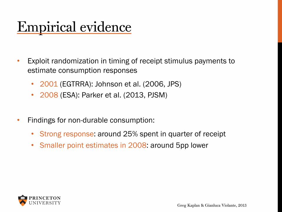
Empirical evidence

•  Exploit randomization in timing of receipt stimulus payments to estimate consumption responses

•  2001 (EGTRRA): Johnson et al. (2006, JPS) •  2008 (ESA): Parker et al. (2013, PJSM)

•  Findings for non-durable consumption:

•  Strong response: around 25% spent in quarter of receipt •  Smaller point estimates in 2008: around 5pp lower


Challenge for standard theory Permanent Income Hypothesis (PIH) •  Zero response to anticipated transitory windfall



Standard Incomplete Markets Model (SIM) •  Consumption response from liquidity constrained households •  Disciplined by data on net worth •  <10% households constrained èrebate coefficient < 5%



Standard Incomplete Markets Model (SIM) •  Consumption response from liquidity constrained households •  Disciplined by data on net worth •  <10% households constrained èrebate coefficient < 5%

Kaplan and Violante (2013) (KV13) •  2 asset model with transaction costs •  Generates wealthy hand-to-mouth households •  Disciplined by data on liquid and illiquid assets •  Parameterized to match 2001 SCF data èrebate coefficients

closer to empirical estimates of JPS


Our objective

Use KV13 framework to shed light on the difference between the consumption responses to the fiscal stimulus policies of 2001 and 2008, as measured by JPS and PJSM


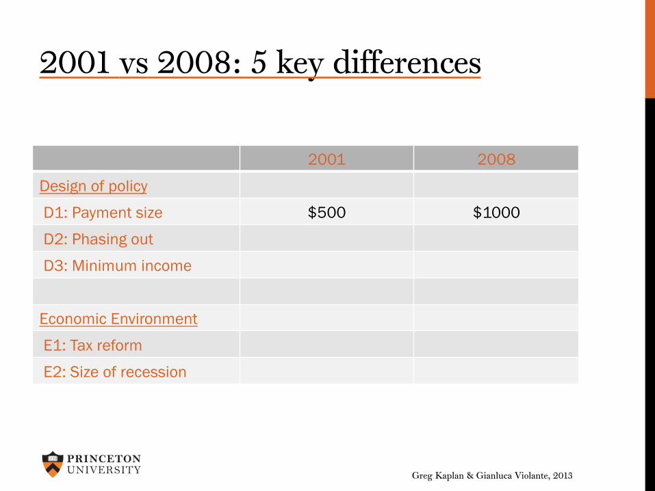
2001 vs 2008: 5 key differences

2001 2008

Design of policy

D1: Payment size $500 $1000

D2: Phasing out

D3: Minimum income

Economic Environment

E1: Tax reform

E2: Size of recession



2001 2008

Design of policy


D2: Phasing out none starting at $75K

D3: Minimum income


E1: Tax reform




2001 2008

Design of policy



D3: Minimum income none at least $3K


E1: Tax reform




2001 2008

Design of policy





E1: Tax reform Bush tax cuts none




2001 2008

Design of policy





E1: Tax reform Bush tax cuts none

E2: Size of recession short and shallow long and deep


Model •  Baumol-Tobin model of money demand integrated into a partial

equilibrium, life-cycle, incomplete markets economy

•  Finite horizon

•  Idiosyncratic fluctuating labor income while working •  Social security benefits when retired

•  Epstein-Zin-Weil preferences defined over

•  Non-durable consumption •  Housing services

•  Two assets:

•  Liquid asset with low return (rm) •  Illiquid with higher return (ra) and housing service flow (³)

•  Depositing or withdrawing from illiquid asset requires paying a fixed transaction cost (·)

•  Unsecured borrowing in liquid asset at rate rb > rm


Parameterization

Preference and risk parameters as in KV13 (2001 steady-state):

•  CRRA = 4 •  IES = 1.5 •  Discount factor (¯) to match median illiquid wealth •  Earnings risk is unit-root


Parameterization

Real asset returns (after tax, annual) as in KV13:

•  Liquid assets: cash; money market, checking, savings and call accounts; directly held mutual funds, stocks, bonds, T-bills; net of revolving debt on credit card balances: –1.48%

•  Illiquid assets: net housing wealth, retirement accounts, life

insurance, CDs and savings bonds: 2.29%

•  Housing service flow: maintenance, insurance, property taxes, interest; imputed rent, tax deductability: 4% of stock


Parameterization

Transaction cost (·) and borrowing rate (rb)

•  Match fraction of wealthy and poor hand-to-mouth (2001 SCF)

•  In KV13 outline strategy for identifying a lower bound:

•  20% - 40% of US households are hand-to-mouth •  1/3 of these are poor, 2/3 are wealthy

•  Target upper end of range: · = $1000 and rb=15.5%

•  In KV13 we target middle of range: · = $1000 and rb=10%


Experiment

•  Replicate 2001 tax rebate episode in model

•  Economy is in steady-state when hit with three pieces of news:

1.  Recession of depth and length of 2001 downturn 2.  Tax reform that mimics EGTRRA 3.  $500 tax rebate to half the population immediately, and to

half the population in the following quarter

•  Compute transition and run JPS/PJSM regressions on model-generated panel data to compute rebate coefficients

•  Repeat experiment with 5 differences for 2008


Model rebate coefficients: 2001 vs 2008

Baseline calibration · = $1000 rm = 15.5%

KV13 calibration · = $1000 rm = 10%

2001 0.271

Design of policy

D1: Payment size

D2: Phasing out

D3: Minimum income


E1: Tax reform


2008: D1+D2+D3 + E1+E2





2001 0.271

Design of policy

D1: Payment size 0.178

D2: Phasing out

D3: Minimum income


E1: Tax reform


2008: D1+D2+D3 + E1+E2





2001 0.271

Design of policy


D2: Phasing out 0.271

D3: Minimum income


E1: Tax reform


2008: D1+D2+D3 + E1+E2





2001 0.271

Design of policy



D3: Minimum income 0.265


E1: Tax reform


2008: D1+D2+D3 + E1+E2





2001 0.271

Design of policy





E1: Tax reform 0.241


2008: D1+D2+D3 + E1+E2





2001 0.271

Design of policy






E2: Size of recession 0.309

2008: D1+D2+D3 + E1+E2





2001 0.271

Design of policy






E2: Size of recession 0.309

2008: D1+D2+D3 + E1+E2 0.187





2001 0.271 0.150

Design of policy

D1: Payment size 0.178 0.119

D2: Phasing out 0.271 0.150

D3: Minimum income 0.265 0.136


E1: Tax reform 0.241 0.163

E2: Size of recession 0.309 0.184

2008: D1+D2+D3 + E1+E2 0.187 0.108


Conclusions

•  Use KV13 framework to shed light on differences in consumption responses to the fiscal stimulus policies of 2001 and 2008

•  3 differences in policy design •  2 difference in economic environment

•  Combined effect: consumption response lower in 2008 by 1/3

•  Most important effect is the larger average payments in 2008

a tale of two stimulus payments: 2001 vs 2008 · a tale of two stimulus payments: 2001 vs 2008...

Documents