A Systems Engineering Approach to Electro-Mechanical Reconfiguration

for High Mobility Autonomy

R. Craig Coulter CMU-RI-TI-94-27

The Robotics Institute Carnegie Mellon University

Pittsburgh, Pennsylvania 15213

August 15,1994

0 1994 Carnegie Mellon University

This research was sponsored by ARPA. under contracts “Perception for Outdoor Navigation” (contract number DACA76-89-C-0014, monitored by the US Army TEC) and “Unmanned Ground Vehicle System” (contract number DAAEO7-90-C-R059. monitored by TACOM). Views and conclusions contained in this document are those of the author and should not be interpreted as representing oficial policies. either expressed or implied. of ARPL4 or the United States Government.

Abstract

The performance of n system is a function of the performance of each of its individual componenls. This wurk explores the relationship between system performance and subcomponent performance in the electru-mechanical configuration of a mobile robot, under the premise that the performance of the mobile robot can be greatly improved through the systematic analysis and design of an efficient electro-mechanical configuration. This work further presumes that the concept of mobiliv adequately encompasses the memcs by which complete mobile robotic systems may be. measured: the purpose of building a mobile robot is assumed to be the creation of a maximally mobile autonomous machine.’ The performance cost of converting an existing machine into an autonomous machine is then measured by its mobility degredation.

This paper develops a methodology that helps the design engineer to reduce one mobility performance cost, and illustrates this method with its application to the NavLab U mobile robot. The conclusion of this work is that the state of the art in mobile robotics is not accurately reflected in the performance capabilities of mobile robots developed primarily to support software research programs. Even a rudimentary first cut at the systematic engineering of performance has yielded a power to weight ratio change on the order of 10%. This study predicts changes on the order of 20% through the implementation of robust low-technology solutions. The development of robust Geld and mobile nbo t s calls for such an engineering approach.

1. In fact. autonomy is considered to be simply another form of mobility - a cognitive form

Table of ContenY

1 .0 1.1 I .2 I 3 I .4 I .5 I .6 I .7 I .8 I .9 1.10 2.0 2.1 2.2 2.3 2.4 2.5 3.0 3.1 3.2 3.3 3.4 4.0 4. I 4.2 4.3 4.4 4.5 4.6 4.7

4.9

5.1 5.2 5.3 5.4 5.5 5.h 5.7 5.8 5.9 5.10 6.0 6.1 6.2 6.3 6.4 7.0 7. I

4.8

5.0

Introduction Acknowledgements Historical Perspcctive A Definition of Mobility Reconfiguration for Autonomy Autonomy Cost of Autonomy Motivation and Goal The Approach and Research Content of the Work The Results of the Work Overview of Conclusions Cost Functions and Performance Metrics for Reconfiguration Cost Functions Configuration Capability Configuration Efficiencies Component Addition and Il The Power Weight Spiral Explained Design for Recontiguration Design Philosophy Goals of Design for Reconfiguration Principles of Design for Reconfiguration n - Based System Analysis n . Rased System Analysis of the NavLab I1 The Functional Design Work;lbility Cost Metric Measure of Workability Measure of Weakness The A, Cost Function Primary Group Cost Functions Cost Function Qualitative Analysis Cost Function Quantitative Analysis Identification of Relevant Technologies Principles of Thermodynamics and Heat Transfer First Law and the Cognitive Thermal Load Partitioning a Thermal Space and the Claussius Statement Thermal Sources Thermal Sink Forms of Heat Transfer Conduction Convection Radiation Thermal Space Heat Transfer Design Goals Convection Cooled Electronics Rack Original Configuration Component Elimination and Substitution Component Addition Heat Transfer Air Conditioned Electronics Rack Original Configuration

3 3 3 4 5 5 5 5 6 7 7 8 8 9 IO 11 12 15 15 15 16 16 17 17 18 18 18 19 19 20 22 23 24 24 23 24 25 25 25 25 26 26 27

28 28 28 28 29 29

28

7.2 7.3 1.4 7.5 7.h 8.0 8.1 8.2 8.3 8.4 8.5 8.6 9.0 9.1 9.2 9.3 9.4 10.0 10.1 10.2 11.0 12.0

Design Goals Specification Assumptions Heat Load Analysis Cost Sensitivity Experimental Validation Summnry of Savings fmm Reconfiguration Air Crinditioning Power System Stager Change Out Structural Changes Summary Comments Concept Configuration Designs Conce.pt # I : Off-load Passengers and Data Displays Concept #2 Eliminate Air Condilioning Concept #3: Production Computing and Sensing Summary of Concepts Summary and Conclusions Summary Conclusions Future Work Ref e I en c e s

29 29 30 31 32 34 34 34 34 34 34 35 36 3h 37 38 39 41 41 41 42 43

List of Fieures

I NavLab I1 2. Elcctr(lnic5 Racks 3. Autonomy Hardware Schelndlic 4 The HMMWV Thermal Space 5 . Convection Cooled Electronics Rack 6. Air Conditioned Electronics Rack 7. Experimental Air Conditioning Apparatus

17 17 19 26 28 29 32

List of Tables

1. Total Heat Load 2. Current Design Weight and Power Savings by Sub-System 3. Current Design Power and Weight Change 4. Component Power and Weight Reductions 5 . Power and Weight Change - Concept # I 6. Air Conditioning Power and Weight Reductions 7. Power and Weight Change - Concept #2 8. Production Computing and Sensing Contiguration 9. Power and Weight Change - Concept #3 10. Design Performance Comparison

31 35 35 36 36 37 31 38 38 39

3

1 .O Introduction

This work adopts an engineering perspec.tive on a topic that has generally been considered to be science - the development of competent mobile robots. The purpose of the work is to determine the degree to which mobile robot performance is affected by the addition of computing, sensors, and support equipment to an existing machine - a process called reconfiguration. It will be shown that the reconfiguration process can have great impact on the performance of the machine, and thus the overall performance of the mobile robot system.

The work's most fundamental premise is that the concept of mobility adequately encompasses the metrics by which complete mobile rohotic systems may he measured. The purpose of building a mobile robot is assumed to he the creation of a maximally mobile autonumous machine.' The performance cost of converting an existing machine into an autonomous machine can then be measured by its mobility degredation. This paper devrlops a methodology that helps the design engineer to reduce this performance cost, and illustrates this method with its application to the NavLab 11 mobile robot. Th is work will stress process refinement over conceptual innovation - the steps necessary to equip a machine for autonomy are nearly self evident. however, the process by which a high performance mobile robot is produced are more obscure.

1.1 Acknowledgements

This academic work grew out of an engineering effort sumunding the NavLab 11 mobile robot. The [ram that perfmned the electro-mechanical reconfiguration included George Mueller, Jeremy Amstrong, Alex MacDonald, Joe.d Haddad, Jim Fmzier, Jim Moody, Bill Ross, Joe Oliver? Travis Schluessler. Bob Shush . Henein Simon and random people from around the FRC and VASC who donated their time and energy. They are all appreciated.

Chuck Thorpe. Tony Stentz, Marrial Hebert and Dean Pomerleau recognized the need to improve the hardware configuration for many reasons; each offered many practical suggestions and the support necessary to form and fund the reconfiguration team.

Many of the practical ideas for restructuring the power system and eliminating components were first suggested by George Mueller. Alex MacDonald and Joed Haddad produced the detailed component redesigns, and performed the fabrication and integration of much of the power generation and contml electronics.

Jim Frazier deserves special mention for his unceasing loyalty to the improvement of the NavLab 11. Jim was one of the last remaining members of the original NavLab team and was key in explaining the reasoning behind the original design as well as methods for improving it. Jim also contributed heavily to the design and development of the latest NavLab 11 - h e was the huh for all of our activity.

This paper benefitted from many long, tiresome and abstract conversations with Alonzo Kelly. He belped me to formulate the engineering bent and suggested long ago that there were probably only one or two fundamental ideas behind all of this reconfiguration stuff, the rest being mere detail. I have to thank AI for his usual detached view.

1.2 Historical Perspective

Mobile robotics Enjoys a relatively youthful existence in the history of science. finding its conc.eption in the artificial intelligence movement in the late 1960's. The earliest forms of mobile robots were machines whose sole puTose in life was to provide the physical means for testing the concepts of vision and reasuning algorithms. About a decade later, another group of mobile robots came along. Decidedly less intelligent than their AI lab cousins, field robots were typically teleoperated, but they proved far more capable of performing useful work. These early mobile robots spurred interest among both military and civilian research agencies. The military saw intelligent unmanned systems as an effective tool for reconnaissance, resupply, medical evacuation and ordnance delivery that lowered the exposure uf human pcrsonnel. A variety of civilian agencies took interest in mobile robots for applications ranging from

I. In fact. autonomy is considered to be simply another form of mobility - a cognitive form

4

NASA's hopes of autonomous planetary exploration to the desires of some transportation agencies to make more efficient use of the current highway infrastructure through high-speed highway autonomy. To each of these agencies. mobile autonomy offered either more efficient use of an expensive resource or the reduction of risk to humans.

Research i n the mid 1 Y 8 O s moved toward a hybrid robot - one possessing the intelligence of the A I lab robots and the physical hardiness of the field robots. Depending upon me's point of vieni the goal was either to make smart robots mure capable ur to make capable robots smarter. Regardless of the viewpoint. the result was the same. A more intelligent version of the field or mobile robot evolved, capable of lengthened excursions on roadways and some limited ahility to challcnge off-road terrain. The first complete mobile robot systems. Shakey and Flake?. (Nilson(91) w'ere developed at the Stanford Research Institute (SRI) in the late 60's. Early mobile robots were characterized by mobile wheeled platforms operating in a fairly benign environment (flat, solid floors peppered with obstacles) and at low speeds - 5 hours to move 20 meters for the Stanford Cart (Moravec[X]). After these initial successes, Carnegie Mellon launched an outdoor navigation effort to test vision algorithms developed for road following - the road being the first logical outdoor testing ground. The experiments were first performed on a six-wheel. skid-steer cart called the Terragator (Kanadel41, Whittaker[l6]), and later on the NavLab (Shafer[llI. Thorpe[lS]h a computer controlled van. In Germany. Dickmanns and Zapp[3] developed a real-time driving system, based on simple line detectiun algorithms, capable of fullowing roads at up to 100 k.p.h. More recently, Pomerleau[lO] demonstrated neural hosed road following at speeds of up to 60 m.p.h. on the NavLab U. The NavLab program moved into natural terrain i n thc FastNav propram (Singh(l2lj. The vehicle operated off-road on essentially flat terrain at speeds up to 30 m.p.h. In 1987 a software team at Hughes developed a cross country navigation system for use on Martin Marietta's Autonomous Land Vehicle, This system was the first cross country system developed explicitly for usc i n rugged natural terrain. The Hughes system. operating at Martin's Denver test site, managed to detect and avoid natural obstacles such as gullies, ditches and bushes in runs of up to 100 meters (DailyrZ]). The NavLab I1 program's Cross Country Team concentrates fully on rough terrain cross country navigation. In the program's first year, they posted unprecedented 5 and 6 kilometer continuous autonomous runs on a Pittsburgh slag heap.' (Stentz[l3]) During subsequent years, performance improved through increased robustness (Kelly[5][6][7]) and through improved global planning (Stentz[ 141).

Software systems have now improved to the point where it is important to consider how to engineer the electro- mechanics of the vehicle in order to improve overall performance. Previous systems were primarily mobile laboratories - equipment placed in racks in the back of a truck, or mobile bases built up to carry the weight of the system. Now that the software has reached a certain level ofmaturity, it has become important to determine how to configure a vehicle so that it supports the needs of the mission at the lowest possible cost to performance.

1.3 A Definition of Mobility

Mobility is a concept that is used to describe the efficacy with which a powered machine traverses ground. Mobility has many measurements; the mobility metric is often an indication of the mobility characteristics of interest. Characteristics of mobility include, but are not limited to:

Distance range or time range of the machine. -Geometry of the machine and its amenability to terrain traversal

-Ability to climb or to surmount obstacles. *Ability to maneuver. * Speed and I or acceleration of the machine..

* Climatic range of the machine, as measured by temperature, pressure. etc.

This study conccntrates on improving mobility through increased speed and acceleration, by improving power efficiency.

1, The NavLab I1 itself is unprecedented in that it is the first cross country mobile robot to remain cssentially mechanically unchanged from its original configuration.

5

1.4 Reconfiguration for Autonomy

Reconfiguration for autonomyl in the sense of mobile robotics. refers to the alteration of an existing machine with the physical hardware and software routines necessary to produce autonomous motion. The assumption is that the robotics designer is construined to incorporate his or her hardware design into an existing machine. .i\lter;itions to the

2 machine‘ are, at best, minimal; fundamental redesigns of the machine are not possible. Should a fundamental redesign he required in order to automate the machine, the design and development process is no longer considered to he a reconfiguration of an extant design; it is the production of a new design.

1.5 Autonomy

Autonomy may be interpreted to mean either physical uuionumy or cognitive uutunomy. Mobile robots are typically considercd to he machines that are capable of some degree of cognitive independence. Autunomous mobile robots are those that exhibit the highest degree of cognitive independence - at the time of this writing, cognitive autonomy typically includes behaviors such as path and motion planning, object recognition. and rudimentary forms of reasnning. Physical autonomy, within the scope of this paper, refers to the machine’s degree of physical dependence on the world. Mobile robots (autonomous or otherwise) may be divided into two classes of physical dependence.Free mobile robots arc self-contained, self-reliant machines that lack any power infusing connection. Free mobility requires that the machine carry its own source of energy, such as a combustible fuel or a bank of batteries. Mobile robots that are nut freely mobile are usually supplied power through a reiher. Tefhered mobile robots are constrained in their mobility by the length of the tether and its effects on maneuverability. Free mobile robots are the subject of this paper, and so the word autonomous will refer to both physical and cognitive autonomy.

3

1.6 Cost of Autonomy

The support of autonomy requires the emplacement of actuators. sensors and support computing. From the point of view of the host machine, these components present an additional burden. Because the host machine is freely mobile, the components must he transported, powered and cooled using host resources. The cost of autonomy refers to the additional weight and the additional power draw required for autonomy.

1.7 Motivation and Goal

This work is motivated by a study of the electromechanical configuration of the NavLab I1 mobile robot, (Coulter and Mueller[ I]). which indicated that appreciable weight savings and power savings could be achieved with minimal changes to the robot’s configuration. The study determined that:

* 33% of the retrofit weight4 was due to power-generation equipment. * 43.4% (if the average power draw was due to the vehicle is air-conditioning.

Coulter and Mueller’s work was precipitated by the poor acceleration performance of the NavLab I1 mobile robot. Excessive vehicle weight retarded the vehicle’s top acceleration. Terrainability was reduced by both the lack of power and alterations made to the vehicle body5 Reduced weight, and changes in the vehicle geometry were seen as the most efficient route to increasing the overall performance of the vehicle. The authors reasoned that if the air-

1 . Permissible alterations include the emplacement of sensors and mounting brackets. generation of small quantities of additional power, and other such small changes. 2. Fundamental redesign implies that the machine itself would require redesign. examples include alteration of steering method, suspension redesign, redesign of the entire powertrain. 3. Wireless electronic connections are not included, as they are not physically constraining. 4. Retrofit weight includes only the weight of equipment added to the mobile robot. The weight of the original vehicle is not included in this measurement. 5. Externally mounted generators collided with the ground when the vehicle climbed slopes in excess of 22“

6

conditioning requirements for the configuration could be sufficiently reduced, then the power generation equipment might be scaled down, resulting in both power and weight savings.

1.8

The approach of this work is to take afurrctional design and extend its performance through syrems engineering for perforriiunce. Systems engineering is the practice of:

The Approach and Research Content of the Work

Examining the input - output relationships of a system’. - Identifying the contributions of the system’s suhcumponents to this output. a Understanding the intra-system links between the system subcomponents. -Examining the sensitivity of the performance of the output to changes in the performance of system subcompo- nents. * Understanding how the optimization of the system is related to the optimization of the subcomponents. - Forinulating a plan that brings about the greatest change in system output performance.

1.8.1 Using the Engineering Approach in Research

The scientific approach has, for centuries, been the accepted cornerstone of resexch. The scientific approach serves to prove or disprove a hypothesis through experimentation, A concept, the hypothesis, is put forth or asserted. The validity of this hypothesis is tested through experimentation. The result is binary - either an assertion or rejection of the hypothesis. The focus of the scientific approach is on the concepf, specifically on its truth.

The engineering approach seeks to constmcl a system thai meets a set ojspecifirations. A system o f interest is chosen and a set of specifications is put forth as a goal. The relationship between the achievement of a specification and the cost of so doing is knuwn or deduced. Tolerance to specifications are traded off against the cost of meeting the specification as the system is built. The result of the engineering approach is two-fold: a system, optimized to specifications and resources, is produced, as well as an understanding of the relationship between cost and performance. Note that the focus of the engineering approach is on theproduct, speci&ally on its performance.

One further distinction remains. While the scientific approach is almost wholly the product of the research venue, the engineering approach is shared by researchers, developers and engineers. The product of the engineering approach in resedrch is not the product itself, but the insighf into the process of producing a higher-performance product. Research using the engineering method asks the question, “in what way might we improve the performance of this existing concept, such that it meets these needs?” Having made these distinctions. the resedrch content of this work surrounds an investigation of the process by which performance may be designed into an existing concept - namely an autonomous mobile robot.

1.8.2 Justification tor the use of the Engineering Approach

This approach is seen to be appropriate to this workbecause: An engineering approach is systematic. An engineering approach concentrates on the apparatus, not the concept.

The subject of the work is performance, which is inherently linked to engineering practice. * The engineering approach allows for requirement traceability.

- The results of an engineering approach lend themselves ta efficient, repeatable and logically alterable sequences. * The result is both an improved product and a r e swch contribution.

I . In this case; an electromechanical system

7

1.9

The rcsults of this work include an improved product, the NavLab n, as well as a better understanding of the process o f engineering performance in an autonomous mobile robot. First, consider the product results. The NavLab 11 remains unchanged in terms of itsfirnctiun; namely, it serves as a research testbed for both on-road and off-road navigation, providing general support for perception, planning and control software. and general autonomous navigation research. However, the vehicle now exhibits faster acceleration, improved climbing capability, and an improved ability to surmount obstacles.

The following engineering research results have also been produced:

The Results of the Work

1

A set of cost funcIIbns andperformance rnetrics. useful for comparing reconfiguration designs. A model of the rela6r)nships hetween configuration performance parameters, and mobile ruhot performance

* Two models of the so-calledpower-wsigh~ spiral a Positive Feedback model and a Chain Reaction model. - A design met/zodalogy ba?ed on performance analysis.

1.10 Overview of Conclusions

This document will demonstrate the following: - Substantial performance improvements are possible, at low cost. through the systematic application of basic engineering principles. * Simple modelling and analysis of the relationship between system performance and component requirements leads to the qualitative insight necessary to make high-level engineering trade-off decisions. - Current mobile robot designs are not representative of the technological state of the art, as they were built for generalization of function. rather than performance.

1. The specifics of these improvements will be discussed in subsequent serrtions.

8

2.0 Cost Functions and Performance Metrics for Reconfiguration

The performance of a niobile machine can be quantified by the ratio of the generated locomotive powrr to the weight of the machine - this ratio is called the power to weight ratio The power to weight ratio is a good first order approximation. It does not account for changes in power output with such variables as vehicle speed and gear ratios: however. within the scope of this work. it adequately serves the purpose ofqualilatively indicating the appropriateness of design changes. 01- the relative merits of competing designs. In this section, the power to weight ratio of a reconfigured machine will be derived as a function of the power to weight ratio of the original machine altcred by the cost of autonomy.

2.1 Cost Functions

The cost of autonomy can be predicted during the design phase using two cost functions. one for power and a second for weight. In the fkllowing sections. these cost functions are derived; the relationship between weight and power draw is found to be non-linear and possessive of an interesting step like behavior.

2.1.1 Power Cost

The total power cost is the sum of the power cost of those components powered from the vehicle’s main engine and those components powered from an auxiliary on-board power source.

2.1.2 Locomotive Power Cost

The locomotive power Cost is equal to the summation of the power loads of the components that are to be powered by the vehicle’s main engine, pro-rated by the etficiency of the machine’s power generation system.

2.1.3 Auxiliary Power Cost

The auxiliary power cost is equal to the summation of the power loads of the individual components that require auxiliarv Dower. oro-rated by the efficiency of the on-board auxiliary power generation System:

2.1.4 Weight Cost

The total weight cost is comprised of two components, the first is the sum of the weights of the individual components which require power. The second is the weight of the auxiliary power generation system. which is found by sizing the system against the auxiliary power requirement. Because power generation components are available in

9

discrete sizes? the weight of the power generation system is the weight of the. smallest system capable of supplying the auxiliarv power. This relationship is represented bv the floor function.

I J

2.1.5 Cost Duality

Consider the power cost of an individual component i. in the power cost suinmation above. Each component contributes its power cost to the total power cost; however. the power cost of some components is a function of the power costs of other compone.nts. If raising the powerdraw of component A affects the powerdraw of component B, then component A exhibits power cost duality. An example of such a component is a computing card. As the powerdraw of the computing card increases, 50 does its need for air conditioning. Raising the powerdraw of the card may require. i n turn, raising the powerdraw of the air conditioner. The overall effect on the system is inore than just the card’s powerdraw increase.

2.1.6 Generality of the Floor Function

The tlaor function is of general importance in calculating the power and weight costs of a configuration. The floor function, as used in this work, is adapted from the concept of the integer floor function. The integer Door function takes as its input a real number, and returns the smallest integer that is larger than that real number. The selection of a component h l lows a similar vein, and can be expressed with a similar floor function. Let the input to the floor function be called the demand vector, D. The demand vector i s a vector of performance specifications pi, each of which must be met by the component. Let the capability of the component be described by a s imi la capacity vector. C. Le1 the cost of using each component be represented by a cost vector K, whose mciiibers include at least the

I componenl weight.

Weighr D = 11 C = F! K = [Power]

Volrtme ... ...

The general floor function takes as its input a single demand vector, D. and a number of component capacity vectors C,. It returns the smallest cost vector K that corresponds to a capacity vector C whose every member meets or exceeds the corresponding demand (c, > pJ).

2.2 Configuration Capability

The capability ofthe configuration’ is defined by the configuration power to weight ratio. which is found as tollows.

2.2.1 Configuration Power

The configuration power C, is the power generation capability of the original machine. M,. depleted by the locomotive uower cost:

I . I n this work, weight and powerdraw. 2. The cunfipuratiori is the machine after alteration for autonomy.

10

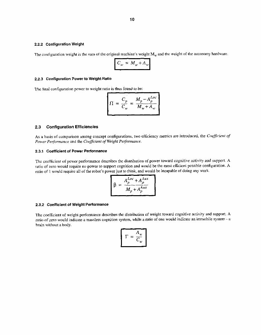
2.2.2 Configuration Weight

The configuration weisht is the sum of the original machine's weight M,v and the weight of the autonomy hardware.

2.2.3 Configuration Power to Weight Ratio

The final configuration power to weight ratio is thus found to be:

2.3 Configuration Efficiencies

As a basis of comparison among concept configurations, two efficiency metrics are introduced, the Crieflcienr of Power Pe&rlonce and the Coejjicienr of Weigh1 Performance.

2.3.1 Coefficient of Power Performance

The coefficient of power performance describes the distribution of power toward cognitive activity and support. 4 ratio o f zero would require no power to support cognition and would be. the most efficient possible configuration. A ratio of I would require all of the robot's power just to think, and would be incapable of doing any work.

M p + A i u x

2.3.2 Coefficient ot Weight Performance

The coefficient of weight performance describes the distribution of weight toward cognitive activity and support. A ratio of zero would indicate a massless cognition system. while a ratio of one would indicate an immobile system - a brain without a bods.

11

2.4 Component Addition and n Consider an expanded form of the configuration power to weight ratio equation.

M , - ( (,)xf'pr:) 1

n =

The form of this equation provides some insights into the nature of n deration as components are added to the configuration. First, note that in the numerator, the configuration power is derated discretely, in an amount proportional to the powerdraw of the individual vehicle-powered components. Second. note that, in the denominator, the weight of the configuration is increased discretely by the weight of the individual components. Finally. note that, in the denominator? the presence of the floor function indicates that the addition of an auxiliary puwered component may or may not further increase the weight of the vehicle configuration.

To summarize, adding a component can have the following effect:

If Dowered b y the vehicle: *Reduces the configuration power.

Adds its own weight to the configuration weight.

If the cumuonent is Dowered bv an auxiliarv source: *Adds its own weipht to the configuration weight. - Increase the auxiliary power load, which MAY force a power and I or weight size up of the power generation system.

If the commnent exhibits cost dualitv it also: - MAY force a power and / or weight size up in a second component.

2.4.1 Cost Duality and Hidden Floor Functions

lf a component exhibits cost duality, it may farce a power and I or weight size up in a second component. Cost duality exists when il second component must be sized to meet the specifications of a group of subcomponents. The given example in this work has been air conditioning. Because the second component is being sized, its power draw and weight ure alsopoorfunctions. The significance of this statement is that in the expanded n equation, fhe individual weighfs )Vi andpower draws Pi may themselves beJhor functions. lending an increasingly complex behavior to the configuration process.

2.4.2 The Significance of the Floor Function -The Straw that Broke the Camel's Back.

The floor function exhibits a step like behavior at its threshold. In practical terms. this means that whether a component addition results in a significant change in n is often more a matter of how close the configuration is to the threshold than on the component itself, This behavior is an instantiation of the straw fhat broke the carne['s back principle.

12

2.5

The power-weight spiral is an effect commonly noted by systems integrators. Occasionally. the addition of component A results in the need to upsize one or more additional cumponents. It is also possible that the upsizing of these additional components will. in turn, cause the performance of componentA to be insufficient. requiring it to be upsized; this results in a positive feedback situation. There are two fundamental types of power-weight spirals. The first i s truly a spiral, and is called the Positive Feedbuk Power-Weight Spiral, The second i s not truly a spiral, i n thc sensc lhat it is not a closed loop response; but merely a chain reaction - this reaction i s called the Chain Reaction Power- W'eighl Sp i rul.

2.5.1 Positive Feedback Power-Weight Spiral - the Power Weight Density

A positive feedback power-weight spiral occurs as a result of internal coupling in t h e n equation. Consider the fullowing simplified version of t h e n equation.

The Power Weight Spiral Explained

I.;] M~ - A,"O~ M w + Aw

Assume now the that value of Il is too low for the needs of the mobile robot; the designer wishes to increase II Further assume that he or she chooses to increase ll by increasing M,,.' Because there is no such thing as a massless power source, increasing Mp necessady affects M , as welt. ?v$ and M, are function;illy coupled. The changc i n Il for a given change in M, can be calculated as follows:

I I

Taking the partial derivatives and noting that there is nu functional dependence of 4, or Ap on M,:

( M , + A,)

The condition for increasing n is found when this partial derivative is greater than zero:'

1. Kote that increasing the auxiliary power c.an only reduce Il as it increases weight without supplying addi- tional locomotive power. 2 . I have omitted some algebraic steps here by noting that the denominator is always positive; I can thus con- sider only the numerator in the inequality.

13

Noting that (M," + 4,) and (hip - AP) are both always positive quantities, the partial derivative may be isolated wifhoul loss of generality:

( M , -A:')

This equation may be inverted to yield the following condition for increasing n with two caveats that will be explored in a moment.

This condition may be interpreted as follows. The ratio of thechange inpowerpmduction to the change in weight must be greater than the current configuration power to weight ratio in order for the addition of the component to increase n An intuitive way to think about this relationship is through adensity analogy. Think ofn as the power Io weight density of the system. Increasing Il means increasing the system density. A density can only be increased by adding something that is more dense to the system. The ratio of change in power to change in weight is the den& of a difffrential quantity The condition requires the density of the differential to be greater than the density of the system,

The positive feedbuck power weight spiral occurs when a power producing component that does not meet the condition is added to the configuration. Instead of raising IJ. as expected, the additional power producing element derates n Positive feedback can OCCUJ if the designers mistakenly continue to add more power producing elements - effectively wonening the situation.

2.5.2 Two Caveats to the Power Weight Density Condition

When the differential quantity was inverted to yield the last equation, there was no consideration given to the possibility that the differential itself could be a negative number, or undefined. I t could be the case that the replacement of a power source with a new power source (such as the replacement of a gasoline engine with a jet- engine) could result in a net power increase and a weight decrease. The case where the partial derivative is strictly negative is therefore an equally acceptable condition, QS h g a the power is increasing. In the case where the ratio is undefined, due to a zero change in weight, the condition i s governed by the sign of the change in power. A positive power change raises n a negative power change lowers The following conditions also lead to an increase in n - Neeative Ratio: due to increasing power, decrease in weight:

L 1

~~ ~~

Undefined Ratio: due to zero weight change. with increase in power.

14

2.5.3 Chain Reaction Power-Weight Spiral - the Floor Function

R chain-reaction type power-weight spiral DCCUIS when one or more cust duality linked components are near their thresholds when a component is added. What appears to he a closed loop effect is actually the result of exceeding severlrl component thresholds one after the other. It is significant to note that small changes in variables (power draw) can result i n large changes in n (power to weight ratio). Note also that the effect (and lhus the spirol) is reversible. If the requirements of a functional design can be reduced by a sniall amount, it i s possible to increase the power to weight ratio by il large amount. Intuitively, this means edging the design under the limits of the next smaller series (thus lighter) of power components. This point will turn out to be key to the application example in this paper.

15

3.0 Design for Reconfiguration

The methodology applied to reconfiguration design is an extension of systems design theory. I t places the fundamental design burden on undersfanding the relalionship between component performance und system pcrforniaace. Once this relationship is understood, it is easier to identify and bolster the weak links i n the reconfigurntion design. The cost phcnornen;i identified io the previous section are useful for quantifying the overall system performance. csrablishing a quantitative relationship between component and syntcm, and for exploiting the non-linear nature of component based designs as exhibited in the floor functions. This section will identify the key issues that arc relevant to producing a performance reconfiguration design. The discussion is necessarily general, however, this section will he followed by a detailed account of the implementation of the method to the NavLab I1 mobile robot.

3.1 Design Philosophy

The design philosophy of this work is to use a systems theoretic approach to alter a functional configuration into a performance configuration in the most efficacious manner possible. The principle components of the philosophy are outlined below.

3.1.1 Functional vs. Performance Design

Afiincrionul design is one whose success criteria are binary - the final design either pertorms a function or does not. A functional design may embody the proof of concept for a new idea, in the form of a prototype. A performance de.rigrr is 1me whose success criteria are measured against a thresholded requirement. Performance design is less concerned with conceptual innovation and more concerned with conceptual refinement. A performance design seeks to push the performance envelop of the functional design. Io see how far the concept can go. Mobile robots have traditionally been functional designs. They halve been built as laboratory test-beds, o r field machines used for software proofs-of-concept. By contrast. this work is not about conceptual innovation, but rather about process refinement.

3.1.2 Relevant Sys tems Design Principles

The design philosophy embodied in this work borrows heavily fmrn and elaborates upon systems design theoy. The examination o f input-output performance relationships and the understanding of intra-system links are basic tenants of systems theory. Informal performance sensitivity analysis techniques are used to decide among potential design changes.

3.1.3 Reworking the Weakest. Workable Link

The performance optimization method used to make design alteration decisions essentially identifies and reworks :he weakest, worknble link. The optimization is a cost-benefit trade-off between weakness and worknbilin;. Weakness is a measure of the degradation with which a component emburdens the system. Workability is a measure of the costs of redesigning the component and of implementing the new design. The output of this process is the component whose cost of redesign is most justified by system performance improvement, essentially the gradient of the weakness - workability space.

3.2

The design philosophy outlined above is without reference to the area of application - reconfigurntion design. In this section. we wish to establish as goals thuse aspects of the design process that are specific or useful to the area of application. The goals of reconfiguration design are to:

Goals of Design for Reconfiguration

-Produce a performance design that minimizes the change to the machine’s original power to weight mtio, while meeting the needs of [he functional specifications.

16

*Provide a method of predicting the cost of adding a component. or the benefit of doing without a component. - Provide a traceable account of the reconfiguration decisions that is useful tix streamlining the design process

3.3

The following rules of thumb hold true across the arena of application. and are useful for the designer to keep in mind:

*The performance of the machine will necessarily deteriorate as a result of the addition of autonomy hardware. * Jt is important to understand the links among component specifications and to identify components that exhibit performance cost duality. * Identify the components with the highest performance sensitivity. *Identify the components that constitute the largest weight and power portions of the autonomy hardware. * Identifj components whose power and weight requirements are dictated by floor functions.

Principles of Design for Reconfiguration

3.4

The primary goal of the design approach is to produce a performance design that minimizes the change to the machine’s original power to weight ratio. Using the following equation of the performance metric n the high-level decision of how best to go about altering Il can be made. Recall that:

n - Based System Analysis

M -ALoc

M,,? +A,

This analysis assumes that there is a cost metric for workability (dollar cost, time cost, etc.) and a benefit metric that describes change in system performance as a function of the change in sub-component performance.

*Write a cost metric for workability in terms of money, time. and other relevant quantities Measure the workability of the components [Mp, M,, Ap, pk), using the cost metric.

*Measure the relative weakness of the components {M,, M, A,, &I.’ * Write A, and 4, components? What is the sensitivity of n to subcomponent changes? * Identify cross-component dependencies? * Identiij the technologies and the risks associated with m&ng a change in each component.’

cost functions and examine the qualitative dependencies. Are there floor functions, cost dual

This systematic procedur-e will help the designer to understand the system and the intra-system dependencies. and provides a traceable account of the performance dependencies. useful for altering future design decisions. One can consider the output of this analysis to be a “big-picture” of the system performance that quantitatively puints out the local improvements most likely to bring about better system-level performance.

I . Which contributes the most to the configuration weight, M, or qV? Is Ap significant compared to M,? 2. For instance, does increasing M, necessarily increase M,? 3. Are the technological upgrades proven and off-the-shelf. are they untested and basic researchq

17

4.0 n - Based System Analysis of the NavLab II

The NavLab 11 is a reconfigured HMMWV military truck that is used as a testbed for both on-road and off-rciad navigational software testing. In this section, a n-based system analysis will be performed o n the NavLab 11, resulting i n the information necessary for a redesign of the system configuration. This chapter will begin with an overview of the original configuration of the NavLab 11.

4.1 The Functional Design h functional design is any design that achieves the design goals, but not necessarily in an optimal fashion. In this section, thc original configuration of the NavLab II mobile robot is assumed as the functional design. The following figure describes the functional layout of the NavLdb IL In this design. the cognitive power is generated by two 5KW I eeneraturs mounted at the rear of the vehicle. Each generator distributes its power to an Uninterruptable Power Supply (UPS) which performs power conditioning and supplies battery backup. The UPS distributes power to the mi-ious electronic components found within the vehicle, including power supplies, mimitors, camera controllers. commter boards. etc.

NavLab I1 Side View NavLab I1 - Rear View

Figure 1: NavLab Il

The electronics components are housed in one of two component racks. The driver's side rack is encloscd and air conditioned. It contains the vehicle computing. disk drives, amplifiers, power supplies and an inertial measurement uni t . The passenger side rack contains video switching equipment, camera controllers, and pan tilt control devices.

Air Conditioned Rack Open Air Rack

Control L Computing i:

............ g

z : ' a :4 . i : airflow: m

............. DiskDrives INS

Figure 2 Electronics Racks

18

4.2 Workability Cost Metric

The workability cost metric for the NavLah I1 mobile robot has three elements. Cost is measured as the linear combination of expected dullarcost. expected timeexpenditure, and the non-relevance to research.' The programmatic goals of the project provided some ahsolute dollar cost and time cos1 ceilings. I n general dollars were found to be more costly than time. while research content was considered more important than bolh dollars and time.

4.3 Measure of Workability

4.3.1 M, and M, Changes to the power production of the vehicle's engine and the original weight of the vehicle were ruled out as too costly for the following reasons. First and foremost, there is little or no mobile robotics reseach content in redesigning the vehicle itself. Secondly, both the dollar and time costs were expected to be high due ti) the mismatch between the orynization and the task - the university is not organized to perform custom automotive redesign. Costs for such a venture are expected to he high due to the steep learning curve and possible required capital equipment investments.

4.3.2 Apand& Changes to the engine power draw were led out because the original configuration drew no power from the vehicle engine, except for three small actuators. The power draw of these actuators is minimized for the application and practically insignificant to the engine. Coulter and Mueller[ll identified in their configuration study likely sources of weight reduction in the autonomy hardware. As as result of process of elimination (there was no less costly alternative) and due to the high likelihood of a performance improvement, 4, was chosen as the single component fiir redesign study.'

4.4 Measure of Weakness

4.4.1 Coefficient of Power Performance

Tl1z cnefficient of power performance is calculated as follows:

This indicdtes that about 3.5% of the power ofthe entire vehicle is dedicated to cognition and cognitive support

4.4.2 Coefficient of Weight Performance

The coefficient of weight performance is calculated as follows:

This indicates that approximately 25% of the total vehicle vreight is dedicated to cognitive support

I , Research non-relevance is a measure of the nature of the work to be undemken. As a university. it is pref- crable to spend time doing work that has mobile robotics research content. It is acost to undertake work that has no research content. 2. Note that in general, more than one component can he chosen for redesign. The selection ot'a singlc coin- ponent is specific to this application.

19

P,,, = 2 6 . CameraController+ 54 . VideoEncoder+ 15 VideoSwitcher

WCcE = 10 CameraController + 8 VideoEncoder+9 . VideoSwitcher -

4.5 The A, Cost Function

Consider the following schematic of the autonomy hardware. This drawing represents the power flow frclm the generator through the U P S , to the electrical components. Components are subdivided into tive primary groups. The 4, cost function can be written as the summation of the weight cost functiuns of each of these five primary groups.

A,, = W CCE + ~ v . 4 4 ~ ~ ~ ~ ~ ~ r ~ 4- + wSemom + wACE+ wUPS + W C r n r r u t o i s ~

Figure 3 Autonomy Hardware Schematic

4.6 Primary Group Cost Functions

In this section. the power and weight cost functions for each of the five primary groups will be given. Some simplifications have been made, usually to prevent a summation from extending beyond a few terms. None-the-less the basic form of each of the cost functions has not been altered in any way. Powers are reported in watts; weights are reported in pounds-force. The cost functions are written to represent the original orfunclional configuration. In later sections, the redesign will be presented a a way of altering these cost functions.

4.6.1 Convection Cooled Electronics The convection cooled electronics rack contains video processing and video control electronics. The cost functions for the convcction cooled electronics x e found to be linear combinations of the individual components. J

I ~

IVMonirors = 55 . Monitor, + 3 0 . Monitor2 + 17 Monitor3 PMOnilorr = 132. Monitor, + 14 . Monitor2 + 33 Monitor3

1, Note that CamcraContruller. VideoEncoder and similar words are variables that denote the number of such components.

20

4.6.3 Sensor s The sensors’ cost functions are also found to be linear summations.

PSCnJ.IjrE = 26 - Camera + 300 Laserscanner + 336 . Staget

W,,,,,,, = 10. Camera + 7 5 . LaserScanner i 317. Staget

4.6.4 Air Conditioned Electronics

The air conditioned electronics’ cost functions are found to be linear summations

I = 20. VMECards + 520 INS + 20 . Sparc t 25 . PowerSuppIies

WAC, = 1 . VMECards + 40. INS + 2 Spare + 7 PowerSupp1ie.s

4.6.5 Air Conditioning The cost functions for the air conditioning are floor functions of a single variable - the power cost of the air conditioned electronics. The air conditioner must be sized according to heat loading requirements. which are functions of the power dissipated by the air conditioned electronics.

4.6.6 UPS and Generator Sizing The UPS and the generators are each sized according to the total power draw of the vehicle system. Their weight cost functions are multi-variable floor functions. The U P S power draw is proportional to the power drawn through the UPS.‘ The generator consumes no power. and so has no power cost function.

4.7 Cost Function Qualitative Analysis Consider the cost functions derived in the previous section. Some qualitative statements can he made concerning the mathematical behavior of the cost functions. These qualitative statement lead to insight into the form of the problem. and thence to appropriate solutions.

I , Due, almost solely, to inefficiencies in the power transformation process.

21

4.7.1 Floor Functions The presence (if floor functions indicates the capacity for sharp changes in the value of the corresponding cost function. There arc two groups that exhibit this behavior:

-The weight and pnwer draw of the air conditioner are both floor functions of the powcr draw of the air-condi- ti oned e lectrci n ics .

machine. The weight of both the generator and the IJPS are floor functions uf the power draw of every component in the

4.7.2 Cost Dual Components The arguments of floor functions exhibit cost dual behavior. Therefore the air conditioned electronics are cost duul with respect to the air conditioner. Every component in the vehicle is cost dual with respect to the generator and the U P S . Note that fhe QW conditimed electronics aclual1.v have two cos1 dual behaviors - once for the air conditioner, and once again for the power generation and conditioning equipment.

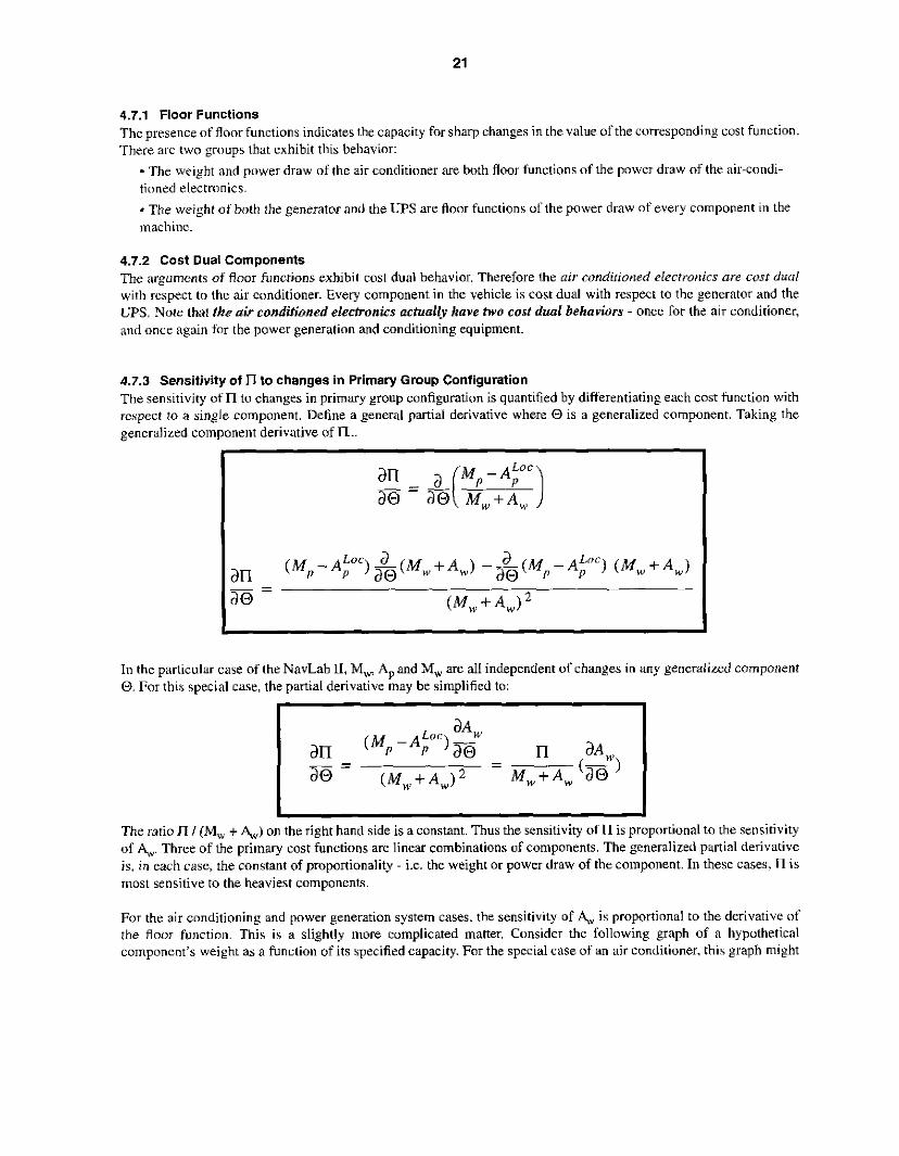
4.7.3 Sensitivity of Il lo changes in Primary Group Configuration The sensitivity of n to changes in primary group configuration is quantified by differentiating each cost function with rcspect to a single. component. Define a general partial derivative where 0 is a generalized component. Taking the generalized component derivative of n..

In the particular case of the NavLab II. M,, A,, and M, are all independent of changes in any generalized component 0. For this special case, the partial derivative may be simplified to:

I 1 The r a t i o n I (M, + &) on the right hand side is a constant. Thus the sensitivity of n is proportional to the sensitivity of .A,v Three of the primary cost functions are linear combinations of components. The generalized pzrtial derivative is; in each case, the constant of proportionality - i.e. the weight or power draw of the component. In these cases. n is most sensitive to the heaviest components.

For the air cnnditioning and power generation system cases, the sensitivity of A,v is proportional to the derivative of the flour function. This is a slightly more cumplicated matter, Consider the following graph of a hyputhetical component's weight as a function of its specified capacity. For the special case of an air conditioner. this graph might

22

relate the weight oftherequired air conditioning unit to the heat generated by the components that it is required to cool.

A Weight

4

b Capacity

The graph shows that the slope of the function is zero, except at discrete points, where it is infinite. The jump in magnitude at these points is given as A and B in this particular graph. This behavior indicates that Il is insensitive to changes in the argument of the floor function, except at these discrete locations. Technically, the deriv-ative is infinite, at the point, however, if a finite capacity difference i s substituted a finite sensitivity may be obtained.

4.8 Cost Function Quantitative Analysis

For the particular case of the NavLah 11, the quantitative values necessruy to make use of the qualitative analysis are available from Coulter and Mueller[l]. But first, consider what was learned from the fortn of the equations. The power generation equipment are rated by floor functions - this indicates that, if the argument of the floor function is near a discontinuity, then it may be possible to drop the number or size of the components. The savings is given by the magnitude at the discontinuity of interest. The air conditioner was also found to be rated by a floor function, where the argument of that function is given by a linear combination of components. Recall also that the air conditioner power draw, (a floor function) is itself an argument of the power generation floor functions. The cost dual components are idcntified as the air conditioned electronics and the air conditioner. This system exhibits the behavior afthe chrrin reuctiori power to weigh? spiral due lo the chninedfloorjimctions.

From Coulter and Mueller[l]. it was found that the weight of the power generation components constitutes 33% of the retrofit weight', and that 43.4% of the average power draw was due to the vehicle is air-conditioning. The current configuration includes two UPS units and two generators. Thus, $ 2 is the case that the power generation floor function is near its discontinuity, then the number of components may be halved, resulting i n a 50% savings. Since the air Conditioning Constitutes a large yonion of the load on the power generation system, it is a likely target for optimization. Recall that the air conditioning rating is itself a floor function, whose argument displays the most significant cost dual nature in the system. The quantitative information also suggests that other cost savings may be accomplished throughout the system. Specifically, the replacement of the Staget (which draws more than 400W) with a lower pow'er functional equivalent could result in a significant power savings.

4.8.1 Design Change Selections

From this quantitative information, specific design changes may now be selected. The first is to redesign the air conditioned electronics package such that a smaller air conditioner will do the job. The second is to identify and perhaps exchange high power draw and I or high weight components throughout the system for more efticient components.

I . Retrofit weight includes only the weight ofequipment added to the mobile robot. The weight of the original vehicle is not included in this measurement.

23

4.9 Identification of Relevant Technologies

At this point. the Il based analysis has completed its function. It has identified the components whose redesign will eflect the most significant change in the system petformance relative lo the workabilily cost metric. Now, the reconfiguration process requires more fundamental engineering analyses. Because this study identified the air conditioner as the principal component requiring redesign, the next sections of this document consider heat transfer and thermodynamic principles as they apply to the minimization of the air conditioning requirement.

24

5.0 Principles of Thermodynamics and Heat Transfer

Thcrrnodynamics conccrns itself with the transfer of energy from one form to another. This transfer of energy is accomplished through two means: work and heat, each of which can be considered a transient form of energy. Wc tend to think of work as an energy transformation that occurs a5 the result of the application of a furce through a distance - or we might also think of it in its contrary form, an energy transformation that occurs without the exchange of mass, or across a temperature difference. Heur. by contrast, is a transient energy form that exists by virtue of a difference in tempcrature hetwcen two system.

5.1 The first law of thermodynamics relates the change of energy of a system to the production of work and I or heat. In the case of a process, the energy E added to a system is balanced by the difference of the heat Q and work W,'

First Law and the Cognitive Thermal Load

[ E = Q - W I

Electronic components do no work on the environment. Specifically, the electronic components do not accelerate any mass through a distance. Thus all of the energy that is consumed by the electronic hardwae is converted to and dissipated as heat. Therefore, the rate of the cugnirive t h e m ! load is the hear equivalent of the cognitivepower lo&.

5.2

The first law requires that the cognitive power load be exhausted as heat. The design is further constrained hy the need to maintain the temperature of the electronic components within the manufacturer's specified range. The components may be partitioned into a small set of thermally separate spaces2 such that these temperature constraints are met. Edch thermal space may either he actively cooled, or exhausted to the environment. If it is necessary to actively cool a thermal space, then we should note that an additional input ofpower i s required; this is formally expressed in the second law of thermodynamics.

There are two classical statements of the second law of thermodynamics, the Kelvin-Planck statement and the Claussius statement, The latter, which is more relevant to refrigeration cycles states: I t is impossible ru construct a device rhar operates in a cycle and produces no efect other than the rmnsfer of heat from a cooler body ro a hotter body. The refrigeration cycle cools by transferring heat from a cool body (the evaporator coil) to a warm body (the condenser coil). The second law is resmctive. requiring the input of work to achieve the heat transfer. Taking the Claussius statement into account, the design goal becomes: arrange the components such that !hey meet the [emperdure constraints while minimizing the active cooling requirement.

Partitioning a Thermal Space and the Claussius Statement

5.3 Thermal Sources

Including the cognitive thermal load (listed as the first two bullets below). there are five general heat sources applied to the vehicle. They include:

* Elcctronics hardware * Power generation and distribution hardware * Solar radiation * Engine I transmission

People

I . The equation is Q - \I' because of the sign conventlon for work. Work done on the environment by thc sys- tem is considered to he negative. 2. It is possible to meet the thermal requirements with a single thermal space.

25

5.4 Thermal Sink The thermal sinks for the vehicle system are free and forced convection to the atmosphere, and conduction through the vehicle body.’ The magnitude of the latter is small compared to the former and is hereafter discounted as a viable sink.

5.5 Forms of Heat Transfer

Heat may be transferred from one system to another through three basic mechanisms: * Conduction: An energy transfer that occurs through the exchange of internal energy between systems. either thrnugh direct contact, or the kinetic energy of molecular motion. or through free electron drift (in t h e c a e of met- als). * Convection: An energy transfer that occurs in Ruids through the mixture of one portion of the fluid with another due to gross fluid m a s motion. Convection may he either free, or forced. In free convection, the fluid motion is caused by means internal to the system. Motion in forced convection occurs due to the application of an cxternal force. such as a fan. -Radiation: An energy transfer that occurs due to the exchange of electromagnetic radiation.

5.6 Conduction

Conductive heat transfer occurs primarily as the result of a temperature difference across a material. If you think about holding an iron bar in a fire, the heat of the fire will flow through the bar to your hand. The rate of this heat flow is dependant upon things like the length of the bar, the temperature of the fire. and the material properties of iron. The law nf thermal conduction is stated as follows:

The heat q, transferred through the cross sectional area A, is proportional to the temperature gradient normal to this area. The constant of proportionality k is called the thermal conductii’iry of the conducting material: i t is the heat transter coefficient for conductive heat transfer.

5.7 Convection Convective heat transfer occurs in fluids (in this context fluid means both liquids and gases) as the result of conduction within the fluid and fluid motion. Heat manifests itself as molecular motion in a nuid - the molecules gain kinetic energy as a result o f heat addition. The motion of the fluid, either due to molecular motion. or gross macroscopic motion, results in the transfer of energy from one portion of the fluid to another. You can think of the Ruid molecules as picking up the heat energy and carrying it through the fluid. If you think about being cooled off hy the wind. the rate of heat flow from your body is dependant upon things like your body temperature, the temperature of the wind, the wind velocity, the angle that the wind makes with respect to your body. your body’s shape, etc.

The transfer of heat through convection is expressed through Newton’s law of cooling:

The heat transfer rate q. per area A is proportional to the difference in temperature between the fluid and the surface across which it flows. The constant of proportionality h is sometimes called thefilm coeficienr or the unit thrrnial cnnducrutice - more commonly it is just referred to as the convective heat trarrsfer coeflicient. h is dependant upon a

I . The vehicle body may act as a thermal capacitor.

26

complex relationship among fluid properties, surface geometries and the hydrodynamics of fluid motion. It is curnnionly found through the results of empirical study and expressed in terms of dimensionless quantities.

5.8 Radiation Radiative heat transfer occurs as the result of the exchange of electromagnetic radiation between bodies. The most common example is the warmth that you feel while standing in the sun. there is no direct contact between you and the sun, but there is an energy transfer taking place across those 92 inillion miles. The hasic law of thermal radiation emission' is the Stephan-Boltzman law:

3 = E d L a This states that the heat transfer rate q per area A is proportional to the fourth power of the absolute temperature of the emitting body. The constant of proportionality 0, is a universal physical constant called the Stephan-Boltzman constant. The constant of proportionality E , is a type of efficiency constant that is dependant upon material and geometric properties; it is called the emissivity.

5.9 Thermal Space Each one of the components in the NavLab 11 uses that power to operate and. in the process. dissipates that power in the form of thermal energy: heat. I n order to cool the interior of the vehicle there IS a cabin air conditioner; in order to cool the interior of the cold cage there is another air conditioner. In addition tu the internal heat generation from the power system (and from people), the vehicle also gains heat through solar radiation and loses heat to convection along the exterior surfaces.

I

t Convectiont

Electronics People I

Figure 4 The HMMWV Thermal Space

I . for ideal blackbody radiation.

27

5.10 Heat Transfer Design Goals

The n-based analysis has indicated that one of the keys to reducing the weight of the vehicle is reducing the power draw of the air Conditioning unit. The air conditioning power draw is a function of the power d r m of the air conditioned electronics (which i s equal to their heat dissipation) and the heat lransfered into the cold cage. The following section will analyze the convection cooled components and the AIC cooled component in order to try to reduce both the internal heat loads and the heat transfer loads that the air conditioning unit s e e s .

20

6.0 Convection Cooled Electronics Rack

Electronic devices that d o not require air conditioning are housed i n the convection cooled electronics rack. Convection may be either free or forced. In the original configuration, fiee convection was chosen. Forced convection is the method preferred in the new configuration.

6.1 Original Configuration

The original configuration consisted of an open aluminum-frame rack, with two 19". 30U compartments sitting side hy side. The left-hand compartment housed a set of 4 video switching unjts, camera controllers, and a 5et of three power supplies. The right hand compartment held two electronic controller boxes for the Staget stabilized sensor platform mounted on the vehicle's roof.

Figure 5: Convection Cooled Electronics Rack

6.2 Component Elimination and Substitution

In the original contiguration, the electronics rack was just over half full of equipment. Through substitution c i f

components, and some rearrangement, the required volume was reduced to a single 1 9 " 30U compartment. The Staget inertially stabilized platform was replaced with a smaller and more energy efficient pan and tilt. This resulted in the replacement of the two Staget electronics boxes u,ith a much smaller (3U) pan and tilt controller. A change out of cameras allowed the elimination of the 3U camera controller, whose space i s now taken up by the addition of a rack mount VCR. The original electronics rack was also eliminated in favor of a lighter, NEMA- 12 enclosed cabinet.

6.3 Component Addition

Some components originally housed in the air conditioned rack have been moved to the convection cooled rack. because they do not require air conditioning. These include arack of three motion control amplifier cards, and power supplies. for the computing and other electronics.

6.4 Heat Transfer

The power consumption of the cage electronics was measured to be on the order of 400 \V, which is exhausted to the exterior of the vehicle, to avoid raising the passenger compartment temperature. A rack-blower system draws air from the top of the rack and exhausts it to the exterior of the vehicle. There was a choice to he made between drawing the intake from the vehicle interior or exterior. The advantage of drawing the air in from the interior is that it is probably cleaner and cooler; however, the cost is that i t puts an additional burden on the passenger compartment air conditioning hy drawing the cool air to the outside.

29

7.0 Air Conditioned Electronics Rack

Electronic devices whose temperature must be regulated are housed in the air conditioned electronics rack.

7.1 Original Configuration

The following d iagam shows the original configuration of the air conditioned cage. The cage was made of structural aluminum with aluminuln panelled sides. The small third level holds power supplies and power switching circuitry. The air conditioning system's evaporator is mounted to the left side of the cage. and bluws cool air out at the top.

L 0 a & F W

Disk Drives INS

Control Compuung

i f a i r Row ~

............

........... ,

I Figure 6: Air Conditioned Electronics Rack

This design suffered from a number of problems: - The cage i s not insulated, presenting an additional thermal load to the air conditioning system. * The air Row pattern is contrary; i.e. warm and cool air Rows collide. *The tnobt temperature sensitive components (the computing cards) are sitting on top of heat producing elements - the INS and the disk drives. - T h e cage contains components that do not require air conditioning, i.e. power supplies.

7.2 Design Goals To improve the condition of the cage, the following changes were made:

* Remove all components that do not require cooling. - Stack components such that the more temperature sensitive components are closer to the air conditioner outflow. *Reduce the width of the cage to a single rack, to improve the airflow and reduce the surface area of the cage.

Insulate the cage.

7.3 Specification Assumptions

To specify the air Conditioning unit, some assumptions were made about the environment: The air temperature inside the vehicle will not exceed 95" E

* The maximum allowed operating ternperature inside the enclosure is 75" E * The convective heat transfer coefficient outside of the cage is 1.6 BTU I hr ft2 'E This is an approximation for still air. * The convective heat transfer coefficient inside the cage is 3.0 BTU / hr f? "F. This is an approximation for air moving at 8 ft/sec. This is probably high since the entire inside area will not see high air movement. * T h e conductive heat transfer coefficient for the insulation is 0.3 BTU I in hr ft' "F. This is a heat transfer coeffi- cient for a commercial insulation called polyimide. There are other products available with both higher and lower coeficients. -The exposed area of the cage is approximated at 32 square feet. Four sides of 6 square feet plus a top and bottom with 4 square feet each.

30

7.4 Heat Load Analysis

Air conditioning units are specified by heat load. Heat loads originate from two sources: internal and external. External loads are also called heat transfer loads. The internal load for this system comes from the contained electruoics. From a previous report, it is estimated to be a maximum of 24UO W. The heat transfer process is a combination of convection (both free and forced) and conduction and can be estimated by:

where: - A is the transfer flux area. * 4 T is the temperature difference. * L the conduction length - I; i s the conductiun coefficient. * h i is the interior convection coefficient.

h, is the exterior convection coefficient

7.4.1 Case # 1: Uninsulated Cage For this case, assume the thermal conductivity k goes to infinity, simplifying the formula as follows:

From the assumed values of the variables. the heat transfer q is found to be 668 BTU I hr

BTU = 668- AAT (32) (20)

h' h, 1.6 3.0

- 4 = - - 1 1 h r -+ - -+ -

7.4.2 Case # 2 Completely Insulated Cage For this case, assume that the cage is lined with first a half inch. and then an inch of insulating material. Returning lo the general formula and substituting the given values of the variables. the heat transfer for a half an inch of material is found to be 244 BTU I hr. For an inch of insulating material, the heat transfer is 149 BTU I hr.

BTU = 244- - ( 3 2 ) (20) - AAT

1 0.5 1 k r + - + - - + - + - - hi k h, 1.6 0.3 3.0

q = 1 L 1

BTU = 149- - (32) ( 2 0 ) - AAT Y = l L 1 1 1.0 1 hr - + - + - -+-+-

hi k h, 1.6 0.3 3.0

31

Completely Insulated Cage

Uninsulated Door

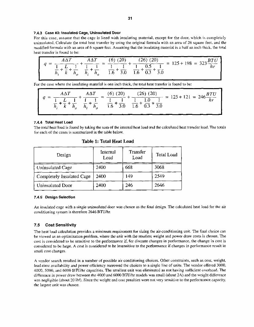
7.4.3 Case #3: Insulated Cage, Uninsulated Door For this case, assume that the cage is lined with insulating material, except for the door. which is completely uninsulnted. Calculate the total heat transfer by using the original formula with an area of 26 square feet, and the mudified foimula w,ith an area of 6 square feet. Assuming that the insulating material is a half an inch thick, the total heat transfer is found to be:

2400 149 2549

2400 246 2646

BTU = 125+ 198 = 323- ( 2 6 ) (20)

1 0.5 1 I I r + - (6) (20 ) - AAT

1 1 + AAT

4 = 1 L 1 1 1 - + - + - - + - - + - - + - + - h, k h, hi h , 1.6 3.0 1.6 0.3 3.0

I I For the cabe where the insulating material is one inch thick, the total heat transfer is found to be:

7.4.4 Total Heat Load The total hear load is found by taking the sum of the internal heat load and the calculated heat transfer load. The totals h r each of the cases is summarized in the table below.

Table 1: Total Heat Load

Design Transfer Total Load Internal I Load 1 Load I I I

Uninsulated Cage 1 2400 I 6 6 8 I 3068 I I I

I I I I I

7.4.5 Design Selection

An insulated cage with a single uninsulated door was chosen as the final design. The calculated heat load for the air conditioning system is therefore 2646 BTUhr.

7.5 Cost Sensitivity The heat load calculation provides a minimum requirement for sizing the air-conditioning unit. The final choice can be vicwed as an optirnization problem, where the unit with the. smallest weight and power draw costs is chosen. The cost is considered to be sensitive to the performance if. for discrete changes in performance, the change in cost is considered ro be large. A cost is considered to be insensitive to the performance if changes in performance result in small cost changes.

A vendor search resulted in a number of possible air conditioning choices. Other constraints. such as cost. weight, lead-time availability and power etficiency narrowed the choices to a single line of units. The vendor offered 3000, 4000. 5n(H), and 6000 BTU/hr capacities. The smallest unit was eliminated as not having sufficient overhead. The difference in power draw between the 4000 and 6000 B T U h models was small (about 2.4) and the weight difference was negligible (aboul20 Ibf). Since the weight and cost penalties were not ver?; sensitive to the performance capacity the largest unit was chuseo.

32

-

33

7.6.2 Experiment # 2 1200 Watts, 78" Ambient Temperature

In this experiment, at an ambient temperature of 78", the heat load was raised to 12OOW and a similar experiment oerfrmned. First, the test enclosure was cooled to a maximum low, and then the heat sourcc was turned on.

7.6.3 Experiment #3: 120* Ambient Temperature

I n this experiment, the ambient temperature was raised to 120" and the air conditioner turned on. When the cage temperature dropped to about 7S", a 67SW heat load was applied

I

7.6.4 On-Vehicle Use

The air conditioning system has been used successfully over a 6 month period. During high humidity days when the temperature reached over 98°F. the inside of the cage remained below 65°F. The power draw inside the cage i s currently at about 65% of the expected maximum.

34

8.0 Summary of Savings from Reconfiguration

8.1 Air Conditioning

The original air conditioning system was a 13,200 BTUlhr system with a separate roof-mounted compressor1 evaporator and side-of-rack-mounted condenser. The new air conditioner is an a l l -bone side-of-rack-mounted 6000 BTUhr uni t , which saves upproximutely IW lbfover the old system. The new air conditioning system draws 1200W compared to the 18(1oW drawn by the former system; however, this i s not a very accurate power comparison. The Components i n the new cage has been arranged in such a manner as to make air-conditioning virtually unnecessdry, The air conditioner runs only when the vehicle is taken out in very hot and dirty environment. When the vehicle is operating while inside the garage, or outside during on-road runs, or when the ambient temperature is in the upper l o ' s or below. the air conditioner is unused.

8.2 Power System

The power system components of interest are the generators and UPS'S. From an earlier study (Coulter & MuellerllJ)l it was found that the total power draw of the original configuration was 4.1 KVA, technically under the limit of the 5 KVA air conditioning unit; however, the power could not be split into two 2.5 KVA legs because of the excessive consumption of the air conditioning unit. This power draw, combined with a design plulosophy oriented more toward expendability that performance. led to the dual generatorRiPS configuration. The new power draw is an average of 3150 KVA. resulting in an average savings of 950 KVA. The total mass loss due to the loss of the generator and UPS is approximately 500 Ibf. An additional 100 - 125 Ibf in structure was also removed for a total savings of about 600 Ibf. This constitutes approximately 40% of the total weight savings.

8.3 Staget Change Out

The Staget pan and tilt system was replaced by a small, light weight, low power system. The Staget offered inertial sensor stabilization. which was found to be unnecessary. The weight savings between systems is approximately 400 Ibf, which constitutes approximately 28% of the total weight loss. The power savings is approximately 340 W.

8.4 Structural Changes

Structural modifications including new cages, the elimination of one passenger station, the elimination of unneeded bracketry and other minor modifications resulted in a weight savings of approximately 300 Ibf - approximately 20% of the total weight savings.

8.5 Summary

The original mobile robot total weight was 10,200 Ibf. The after-reconfiguration tomi weight is 8800 Ibf, resulting in a net loss of approximately 14UO Ibf. The total power draw reduction was only about 950 KVA; however transient

Percentage

Weight Loss weight Of Total Sub-System

Air Conditioning 100 lbf 7.14%

Power 600 lbf 42.86%

Percentage

Reduction PowerDraw Reduction

PowerDraw of Total

600 W 63.0%

-0 0

The effects o f the reconfiguration are summarized below. Aut. Power stands for the power draw of the on-hoard autonomy hardware. Aut. weight is the weight of the autonomy hardware. Vehicle power is the power rating of the vehicle's engine. Weight is the total system weight.

Table 3: Current Design Power and Weight Change

~~ ~

Staget 390 Ibf 27.86% 336 W 35.0%

Structure 3 IO Ibf 22.14% 0 0

Totals I14001bf II 100% I936 W 198.0%

Aut. Power

Aut. Weight I I

Original Modified Percent Total Total Change

4100 W 3150 W -23.17%

2500 Ibf 1100 Ibf -56.0%

Power I I5OHP I 150HP 1 Vehicle

I I I

Weieht 1 10.200 Ibf 1 8800 Ibf 1-13.73% - I I I

n II 0.015 11 0.017 )I +12.0%

8.6 Comments

The change in n is significant, Qualitatively the vehicle feels far more powerful than in i t s previous state. Recall that horsepower is proportional to the product of the vehicle speed and vehicle acceleration. An increase of 12% indicates that the vehicle has, at a given speed, roughly 12% more acceleration. I would also like to note that the redesign changes that brought about this savings were relatively trivial. They required component rearrangement, and a few component substitutions. It is important to note that these changes were low tech improvements to the mobile robot.

36

Weight

9.0 Concept Configuration Designs

The rcconfiguration design that was performed on the NavIab II has, inherently, a number of assumptions about the mission of the vehicle. and its support requirements. Broadly stated, the NavLah series of mobile robots were designed as software development tools - a mobile NAVigational LABoratory for mobile robotics research. As such, this required the emplacement of seats, monitors, computing stations and other equipment for the researcher’s use. The current design still reflects the philosophy of supporting research at the expense of performance. I n this section; we will consider a series of conceptual configurations that undo some of the major assumptions in this philosophy. The perfomance cost of each assumption can then be calculated in several ways. The cost of the assumption in t e n s of the change in n from the original vehicle will be considered, as well as the change in n from the last concept configuration in the series. The conclusion of this section is that the current implementation of nulonomy does not nccurutely refled its currentperfomnce CQpQbi~iikS.

Power

Video Switchers & VCR

Resize UPS

I I

Original I 11OOibf I3150W

-46 Ibf -75 W

-50 Ibf -0

- I I

Monitors I -157 lbf 1-371 W

Resize Generators

I I I I

-30 lbf -0

I Seats and Structure I -1501bf 1-0 I

Modified Total

Aut. Power 3 150 W

I I I I

Concept #I Percent Total Change

2704 W -14.16%

Aut. Weight

Vehicle Power

I I

1100 Ibf 667 lbf -39.36%

150 HP 150 HP 0%

Weight 1 8800 Ibf 1 8367 Ibf I -4.9276 1 n 1) 0.0170 ) I 0.0179 I I +5.3%

37

Aut. Power

Aut. Weight

Vehicle Power

From Table 5 , i t I\ seen that a performance increase of 5 % over the new (here called the modified) cunfiguration results directly froin removing the human h m the environment.

Modified Concept #2 Percent Total Total Change

3150 W 1504 w -52.25%

1100 Ibf 3491bf -68.27%

150 HP 150 HP 0%

9.2

The current configuriltion does not require air conditioning to cool the computing. if adequate air circulation is maintained. The computing is capable of running on 100" days, as long as the heat is properly ducted away from thc electronics. Air conditioning is required only when the computing environment must be sealed from the ambient environment. This is not necessary. as ambient air could be adequately filtered for cooling purposes. The following tables consider the savings incurred by eliminating the air conditioner.

Table 6: Air Conditioning Power and Weight Reductions

Concept #2 Eliminate Air Conditioning

Weight

n

Power

-1200w

8800 lbf 8049 lbf -8.53%

0.0170 0.0186 +9.41%

Resize UPS -120 Ibf

Resize Generators -68 lbf

Total 349 Ibf 1504W

Table 7: Power and Weight Change - Concept #2

9.3

The sensing equipment aboard the NavLab 11 is research grade, which means that it is larger, heavier and most power hungry than would be seen on a production line system. The following power and weight improvements are based on the latest, compatible laser scanning devices and video cameras.

Concept #3: Production Computing and Sensing

Table 8: Production Computing and Sensing Configuration

Generator

Total

Power Weight

28 lbf

Sensing 20 lbf

50 Ibf

0 51

I416 W I 149 lbf

- ~

Modified Concept #3 Percent Total Total Change

Aut. Power 3150 W 416 W -86.79%

Table 9: Power and Weight Change - Concept #3

Weight 8800 lbf 7849 lbf -10.81%

I Aut. Weight I 1100lbf I 149 lbf I -86.45% I

n I / 0.0170

I I I

Vehicle I 150HP I 150HP I O %

Io.0191 I +12.35%

I Power I

39

9.4 Summary of Concepts

The following table compares the six design variation across a number of parameters. An and the percent changc in ll from the original state of the vehicle are all given. In addition, the power performance coefficient B, and the weight performance coefficient r, are all calculated for each design.

Table 10: Design Performance Comparison

Concept #3

Unaltered Vehicle

0

Concept Concept Modified Original #2 #1 Design Design

1504 W 2704 W 3150 W 4100 W

349 Ibf 667 Ibf I100 Ibf 2500 Ibf

416 W Aut. Power

Aut. Weight 0 149 Ibf

Vehicle Power

150 HP 150 HP 150 HP 150 HP 150 HP 150 HP

8049 Ibf 8367 Ibf 8800 Ibf 10,200 Ibf

0.01864 0.01793 0.01705 0.01 47 1

7700 lbf 7849 Ibf Total Weight

n 0.01948 0.01911

0 -0.00037 -0.00047 -0.00071 -0.00088 -0.00234

95.69% 92.04% 87.53% 75,51% 100% 98.10%

0 0.00370 0.01326 I 0.02359 10.02738 I 0.03534

r 0 0.01898 0.04336 0.07972 0.12500 0.24510

9.4.1 Graphical Comparsions

The relationships among power, weight and system perfomance are more readily seen in the following graphs. The p and r plots below show that the weight increase does not follow that same rate as the power increase. Notice that the slopes of the curves do not correlate. Sharp increases in weight coefficient do not necessarily follow from sharp increases in power coefficient.

Power and Welg’lt Zccfficien7,s of Performance

- - - 2 0.10

I- ,>.%- ,An &;- -,

40

The following graphs compare the system performance, n against the total system weight and the total system power draw Note that the performance drop follows precisely from the weight increase , howcver neither Il nor the system w,eight follow the change in power draw.

1

Configuration Comparison

- I % original power to weight r-

Weight (hundreds of pounds)

9.4.2 Comments

These graphs illustrate that, in this case, the relationshp between the system weight and the system power is clearly non-linear. Changes in weight increase in a manner prescribed by the floor functions. Large weight changes correlate to resizing of power components and the elimination of supporting structure. The largest change, between the modified and original designs, corresponds to the doubling of the number of required power components, because physical upsizing of a single component was no longer practical.

I . This is a special case, as no power is being drawn from the engine, the power to weight change is only dependent upon the system weight change.

41

10.0 Summary and Conclusions

10.1 Summary

System performance is inherently an engineering concept and must be designed into an application. The goal of this work was to develop an understanding of the relationship between mobile robot performance (here measured by rl the power to weight ratio) and the support requirements of its sub-components (weight and power draw). The use of a consistent, disciplined, systematic engineering approach provided the framework for developing a high performance design. The following results ensued:

-It was shown that the relationship between system performance and subcomponent support requirements is coin- plicated, nonlinear, and non-intuitive, but rather easily captured in a system performance model. * It was further shown that the system performance model, together with some simple coefficients of performance, are useful for targetting the sub-components whose performance improvement i s critical to system petiormancc improvment.

The performance metrics proved useful in objectively analyzing the costs and merits of concept designs, which gives the designer a foundation for confidently predicting the likely effect of implementing a sub-component rede- sign.

10.2 Conclusions

The foremost conclusion of this work is that the state of the art is mobile robotics is not accurately reflected in the performance capabilities of mobile robots developed primarily to support software research programs. Even a rudimentary first cut at the systematic engineering of performance has yielded power to weight ratio change on the order of 10%. This study predicts changes on the order of 20%, through the implementation of robust low-technology solutions. The development of robust field and mobile robots calls for such an engineering approach.

The application of n-based analysis. or similar systematic analyses, can be done at low cost, with enormous benefit. Simply understanding the qualitiative functional form of system performance enables the engineer to predict the general performance capabilities of a proposed system before committing to the development costs of construction and testing. This is the critical difference between theapplication of the scientific method and theengineering method to this problem. The engineering method is critical to the achievement of capable and robust performance through the application of current mobile robotics technology.

The application of the II-based analysis method to the HMMWV demonstrated that the so-called straw' thar bmke the camel'r back pr inc ip le was responsible for significant performance costs. Simply understanding that such relationships exist and altering the integration accordingly can result in significant performance improvements. the analysis also showed how the performance of the NavLab I1 was effected by a chain reaction pwer to weight spiral. The concept designs showed how such a spiral could be effectively reversed, resulting in large performance improvements at relatively small costs.

42

11.0 Future Work

This method was presented as appropriate to reconfiguration for existing designs. and for the analysis of conceptual designs. It appears to be amenable for original design, where the performance requirements of the mission may be used to constrain the space of candidate mobile robot designs. I would like to apply the method to just such a problenl. I am also curious as to its generality. It was formulated with wheeled and tracked mobile robots in mind, though i t does not appear to he necessarily restrictive. I would like to apply the method ti) the analysis of walking machine configurations to determine the degree of commonality. Finally. 1 would like to extend the approach from power to weight performance to a more general system wide metric or set of metrics. Such an analysis tool wuuld allow the designer to trade-off the requirements of vision sensors, software algorithms, mechanical confizurations. and control systems to arrive at the lowest cost integration that achieves a specified level of system performance.

43

12.0 References

[ I ] Coulter, R. and Mueller, G . “A Reconfiguration Study of the NavLab I1 Mobile Robot.” Robotics Institute technical repurt CMU-RI-TR-94-01.

[2] Daily. M. et al. “Autonomous Cross-Countq Navigation with the ALV”, Proceedings of the 11188 IEEE International Conference on Robotics and Automation.

[3] Dicknranns and Zapp “A Curvature-based Scheme for Improving Road Vehicle Guidance by Coniputer Vision.”> SPIE‘s Cambridge Symposium on Optical and Optoelectronic Engineering, October 1986.

141 Kanade, T. and Thorpe. C. “CMU Strategic Computing Vision Project Report”, CMU-RI-TR-86-2. 1986.

(51 Kelly, A. “A Partial Analysis of the High Speed Autonomous Navigation Problem”. CMU-RI-TR-94- 16. Robotics Institute. CMU, May 2, 1994.

16) Kelly. A. “Adaptive Perception for Autonomous Vehicles”, CMU-R-TR-94-18, Robotics Institute. CMU. May 2, 1994.

[71 Kelly, A. “A Feedforward Control Approach to the Local Navigation Problem for Autonomous Vehicles“, CMU-RI-TR-94- I7,Robotics Institute. CMU May 2, 1994.

[ X I Moravec, H. “The Stanford Cart and the CMU Rover.”, Proceedings of the IEEE, Vol. 71, No. 7, July 1983.

[9] Nilson, N. “A Mobile Automaton: An Application of Artificial Intelligence Techniques.”, Proceedings of IJCAI-69. May 1969.

I IO] Pomerleau, D.A. “Neural Network Perception for Mobile Robot Guidance.” Ph.D Dissertation, Dept. of Computer Science, tech report CMU-CS-92-115.

[ 111 Shafer, S . and Whittaker, W. “Development of an Integrated Mobile Robot System at Carnegie Mellon University: June 1988 Annual Report”, Technical Report CMU-RI-TR-89-22. Robotics Institute, CMU. 19811.

[ 121 Singh; S. et al. “A System for Fast Navigation of Autonomous Vehicles.”. Technical Report CMU-RI-TR- 91-20. Robotics Institute, CMU. 1991.

[ I31 Stentz, A., Brumitt, B.. Coulter, R., Kelly, A., “An Autonomous System for Cross-Country Navjgatjon“. Proceedings of SPIE Symposium on Mobile Robots, 1992.

[ 141 Stentz, A. “Optimal and Efficient Path Planning for Unknown and Dynamic Environment%”. CMU-RJ-TR- 93-20, Robotics Institute. CMU, August 1993.

11 51 Thorpe, C. and Kanade, T. “1987 Year End Report for Road Following at Carnegie Mellon”. Technical Report CMU-RI-TR-88-4, Robotics Institute, Carnegie Mellon, 1988.

[ 161 Whittaker, W. ’Terragator - Terrestrial Navigator” Technical Report, Carnegie Mellon 1984.