a system for acoustic chord transcription and key extraction from audio using hidden markov
TRANSCRIPT

A SYSTEM FOR ACOUSTIC CHORD TRANSCRIPTION AND
KEY EXTRACTION FROM AUDIO USING HIDDEN MARKOV
MODELS TRAINED ON SYNTHESIZED AUDIO
A DISSERTATION
SUBMITTED TO THE DEPARTMENT OF MUSIC
AND THE COMMITTEE ON GRADUATE STUDIES
OF STANFORD UNIVERSITY
IN PARTIAL FULFILLMENT OF THE REQUIREMENTS
FOR THE DEGREE OF
DOCTOR OF PHILOSOPHY
Kyogu Lee
March 2008

c© Copyright by Kyogu Lee 2008
All Rights Reserved
ii

I certify that I have read this dissertation and that, in my opinion, it
is fully adequate in scope and quality as a dissertation for the degree
of Doctor of Philosophy.
(Julius Smith, III) Principal Adviser
I certify that I have read this dissertation and that, in my opinion, it
is fully adequate in scope and quality as a dissertation for the degree
of Doctor of Philosophy.
(Jonathan Berger)
I certify that I have read this dissertation and that, in my opinion, it
is fully adequate in scope and quality as a dissertation for the degree
of Doctor of Philosophy.
(Chris Chafe)
I certify that I have read this dissertation and that, in my opinion, it
is fully adequate in scope and quality as a dissertation for the degree
of Doctor of Philosophy.
(Malcolm Slaney)
Approved for the University Committee on Graduate Studies.
iii

Abstract
Extracting high-level information of musical attributes such as melody, harmony,
key, or rhythm from the raw waveform is a critical process in Music Information
Retrieval (MIR) systems. Using one or more of such features in a front end, one
can efficiently and effectively search, retrieve, and navigate through a large collection
of musical audio. Among those musical attributes, harmony is a key element in
Western tonal music. Harmony can be characterized by a set of rules stating how
simultaneously sounding (or inferred) tones create a single entity (commonly known as
a chord), how the elements of adjacent chords interact melodically, and how sequences
of chords relate to one another in a functional hierarchy. Patterns of chord changes
over time allow for the delineation of structural features such as phrases, sections and
movements. In addition to structural segmentation, harmony often plays a crucial
role in projecting emotion and mood. This dissertation focuses on two aspects of
harmony, chord labeling and chord progressions in diatonic functional tonal music.
Recognizing the musical chords from the raw audio is a challenging task. In this
dissertation, a system that accomplishes this goal using hidden Markov models is
described. In order to avoid the enormously time-consuming and laborious process of
manual annotation, which must be done in advance to provide the ground-truth to the
supervised learning models, symbolic data like MIDI files are used to obtain a large
amount of labeled training data. To this end, harmonic analysis is first performed on
noise-free symbolic data to obtain chord labels with precise time boundaries. In par-
allel, a sample-based synthesizer is used to create audio files from the same symbolic
files. The feature vectors extracted from synthesized audio are in perfect alignment
with the chord labels, and are used to train the models.
iv

Sufficient training data allows for key- or genre-specific models, where each model
is trained on music of specific key or genre to estimate key- or genre-dependent model
parameters. In other words, music of a certain key or genre reveals its own charac-
teristics reflected by chord progression, which result in the unique model parameters
represented by the transition probability matrix. In order to extract key or identify
genre, when the observation input sequence is given, the forward-backward or Baum-
Welch algorithm is used to efficiently compute the likelihood of the models, and the
model with the maximum likelihood gives key or genre information. Then the Viterbi
decoder is applied to the corresponding model to extract the optimal state path in a
maximum likelihood sense, which is identical to the frame-level chord sequence.
The experimental results show that the proposed system not only yields chord
recognition performance comparable to or better than other previously published
systems, but also provides additional information of key and/or genre without using
any other algorithms or feature sets for such tasks. It is also demonstrated that the
chord sequence with precise timing information can be successfully used to find cover
songs from audio and to detect musical phrase boundaries by recognizing the cadences
or harmonic closures.
This dissertation makes a substantial contribution to the music information re-
trieval community in many aspects. First, it presents a probabilistic framework that
combines two closely related musical tasks — chord recognition and key extraction
from audio — and achieves state-of-the-art performance in both applications. Sec-
ond, it suggests a solution to a bottleneck problem in machine learning approaches
by demonstrating the method of automatically generating a large amount of labeled
training data from symbolic music documents. This will help free researchers of la-
borious task of manual annotation. Third, it makes use of more efficient and robust
feature vector called tonal centroid and proves, via a thorough quantitative evalu-
ation, that it consistently outperforms the conventional chroma feature, which was
almost exclusively used by other algorithms. Fourth, it demonstrates that the basic
model can easily be extended to key- or genre-specific models, not only to improve
chord recognition but also to estimate key or genre. Lastly, it demonstrates the use-
fulness of recognized chord sequence in several practical applications such as cover
v

song finding and structural music segmentation.
vi

Acknowledgments
I would like to begin by thanking Julius O. Smith, my principal adviser, who gave
me constant support and all kinds of research ideas throughout the development of
this dissertation work. The enthusiasm and encouragement he has shown through
his courses, seminars, individual studies and a number of meetings inspired me to
accomplish my academic goals. I would also like to thank the other two professors
at CCRMA — Jonathan Berger and Chris Chafe — for their invaluable help and
friendship for these many years through their courses, seminars and research projects.
I would like to thank Malcolm Slaney at Yahoo! Research for his support, supply
of ideas and friendship, which were indispensable in finishing this dissertation work.
My research benefited greatly from a number of project meetings we had together and
from the Hearing Seminar where he invited many expert speakers from all around the
world.
The CCRMA community has always provided me with an excellent research en-
vironment. Especially, I would like to thank my research colleagues and friends in
the DSP group: Ed Berdahl, Ryan Cassidy, Pamornpol Jinachitra (Tak), Nelson Lee,
Yiwen Liu, Aaron Master, Gautham Mysore, Greg Sell and David Yeh for their sup-
port and friendship. Not only their friendship but also research ideas we exchanged
at the regular meetings were invaluable. I am also grateful to my other friends at
the CCRMA, including Juan Pablo Caceres, Michael Gurevich, Patty Huang, Randal
Leistikow, Craig Sapp, Hiroko Terasawa and Matthew Wright.
My thank also extends to the Korean community at the CCRMA: Song Hui Chon,
Changhyun Kim, Mingjong Kim, Moonseok Kim, Dongin Lee, Jungsuk Lee, Zune
Lee, Juhan Nam, and Sookyoung Won. My special thanks go to Woonseung Yeo,
vii

who shared the past five years at the CCRMA as a research colleague, a classmate,
and most importantly, as a true friend.
I would like to thank Lawrence Rabiner at Rutgers University and Juan Pablo
Bello at New York University for their fruitful comments through which my work
could make an improvement. I would also like to thank Markus Cremer at Gracenote
and Veronique Larcher at Sennheiser for giving me opportunities to have real-world
experience via their internships. The internships I did at these places helped me
understand how academic research is actually applied in the industries.
My special thanks go to my parents and my wife’s parents. Their endless love
and support made it possible to complete my dissertation work. My thanks extend
to my two brothers who have been very supportive and encouraging all the time. My
adorable two sons, although they were not always helpful, deserve my gratitude for
just being there with me and for calling me “dad”. Last, but most of all with no doubt,
I would like to thank my lovely wife, Jungah, for her endless support, encouragement,
patience, and love she has never failed to show me during the completion of my work.
It would have been impossible without her. I dedicate this dissertation to her.
viii

Contents
Abstract iv
Acknowledgments vii
1 Introduction 1
1.1 Music Information Retrieval . . . . . . . . . . . . . . . . . . . . . . . 1
1.2 Motivation . . . . . . . . . . . . . . . . . . . . . . . . . . . . . . . . . 2
1.2.1 Content-based Approach . . . . . . . . . . . . . . . . . . . . . 4
1.2.2 Harmonic Description of Tonal Music . . . . . . . . . . . . . . 5
1.2.3 Machine Learning in Music Applications . . . . . . . . . . . . 6
1.2.4 Symbolic Music Documents . . . . . . . . . . . . . . . . . . . 7
1.3 Goals . . . . . . . . . . . . . . . . . . . . . . . . . . . . . . . . . . . . 9
1.4 Potential Applications . . . . . . . . . . . . . . . . . . . . . . . . . . 10
1.5 Organization . . . . . . . . . . . . . . . . . . . . . . . . . . . . . . . 11
2 Background 12
2.1 Introduction . . . . . . . . . . . . . . . . . . . . . . . . . . . . . . . . 12
2.2 Tonality . . . . . . . . . . . . . . . . . . . . . . . . . . . . . . . . . . 12
2.2.1 Perception/Cognition of Tonality . . . . . . . . . . . . . . . . 14
2.3 Computer Systems . . . . . . . . . . . . . . . . . . . . . . . . . . . . 19
2.3.1 Key Estimation . . . . . . . . . . . . . . . . . . . . . . . . . . 21
2.3.2 Chord Transcription . . . . . . . . . . . . . . . . . . . . . . . 27
2.4 Summary . . . . . . . . . . . . . . . . . . . . . . . . . . . . . . . . . 37
ix

3 System Description 39
3.1 Introduction . . . . . . . . . . . . . . . . . . . . . . . . . . . . . . . . 39
3.2 Feature Vector . . . . . . . . . . . . . . . . . . . . . . . . . . . . . . 41
3.2.1 Chroma Vector . . . . . . . . . . . . . . . . . . . . . . . . . . 42
3.2.2 Quantized Chromagram . . . . . . . . . . . . . . . . . . . . . 45
3.2.3 Tonal Centroid . . . . . . . . . . . . . . . . . . . . . . . . . . 46
3.3 Chord Recognition System . . . . . . . . . . . . . . . . . . . . . . . . 49
3.3.1 Obtaining Labeled Training Data . . . . . . . . . . . . . . . . 50
3.3.2 Hidden Markov Model . . . . . . . . . . . . . . . . . . . . . . 54
3.3.3 Parameter Estimates . . . . . . . . . . . . . . . . . . . . . . . 55
3.4 Experimental Results and Analysis . . . . . . . . . . . . . . . . . . . 58
3.4.1 Evaluation . . . . . . . . . . . . . . . . . . . . . . . . . . . . . 58
3.4.2 Results and Discussion . . . . . . . . . . . . . . . . . . . . . . 59
3.5 Summary . . . . . . . . . . . . . . . . . . . . . . . . . . . . . . . . . 62
4 Extension 65
4.1 Introduction . . . . . . . . . . . . . . . . . . . . . . . . . . . . . . . . 65
4.2 Key-dependent HMMs . . . . . . . . . . . . . . . . . . . . . . . . . . 66
4.2.1 System . . . . . . . . . . . . . . . . . . . . . . . . . . . . . . . 66
4.2.2 Parameter Estimates . . . . . . . . . . . . . . . . . . . . . . . 67
4.2.3 Results and Discussion . . . . . . . . . . . . . . . . . . . . . . 70
4.3 Genre-Specific HMMs . . . . . . . . . . . . . . . . . . . . . . . . . . . 73
4.3.1 System . . . . . . . . . . . . . . . . . . . . . . . . . . . . . . . 73
4.3.2 Parameter Estimates . . . . . . . . . . . . . . . . . . . . . . . 74
4.3.3 Experimental Results and Analysis . . . . . . . . . . . . . . . 76
4.4 Summary . . . . . . . . . . . . . . . . . . . . . . . . . . . . . . . . . 80
5 Advanced Model 82
5.1 Introduction . . . . . . . . . . . . . . . . . . . . . . . . . . . . . . . . 82
5.2 Discriminative HMM . . . . . . . . . . . . . . . . . . . . . . . . . . . 82
5.2.1 Experiments and Discussions . . . . . . . . . . . . . . . . . . 84
5.3 Summary . . . . . . . . . . . . . . . . . . . . . . . . . . . . . . . . . 86
x

6 Applications 87
6.1 Introduction . . . . . . . . . . . . . . . . . . . . . . . . . . . . . . . . 87
6.2 Audio Cover Song Identification . . . . . . . . . . . . . . . . . . . . . 87
6.2.1 Related Work . . . . . . . . . . . . . . . . . . . . . . . . . . . 88
6.2.2 Proposed System . . . . . . . . . . . . . . . . . . . . . . . . . 90
6.2.3 Experimental Results . . . . . . . . . . . . . . . . . . . . . . . 91
6.3 Structural Analysis . . . . . . . . . . . . . . . . . . . . . . . . . . . . 96
6.3.1 Related Work . . . . . . . . . . . . . . . . . . . . . . . . . . . 97
6.3.2 Proposed System . . . . . . . . . . . . . . . . . . . . . . . . . 100
6.3.3 Experimental Results . . . . . . . . . . . . . . . . . . . . . . . 103
6.4 Miscellaneous Applications . . . . . . . . . . . . . . . . . . . . . . . . 110
6.5 Summary . . . . . . . . . . . . . . . . . . . . . . . . . . . . . . . . . 111
7 Conclusions and Future Directions 113
7.1 Summary of Contributions . . . . . . . . . . . . . . . . . . . . . . . . 113
7.2 Higher-Order HMM . . . . . . . . . . . . . . . . . . . . . . . . . . . . 117
7.2.1 Introduction . . . . . . . . . . . . . . . . . . . . . . . . . . . . 117
7.2.2 Preliminary Results and Discussions . . . . . . . . . . . . . . 119
7.3 Musical Expectation . . . . . . . . . . . . . . . . . . . . . . . . . . . 121
7.3.1 Introduction . . . . . . . . . . . . . . . . . . . . . . . . . . . . 121
7.3.2 Modeling Musical Expectation . . . . . . . . . . . . . . . . . . 122
7.4 Final Remarks . . . . . . . . . . . . . . . . . . . . . . . . . . . . . . . 123
A Hidden Markov Model 124
A.1 Discrete Markov Process . . . . . . . . . . . . . . . . . . . . . . . . . 124
A.2 Extension to Hidden Markov Models . . . . . . . . . . . . . . . . . . 126
A.3 Elements of an HMM . . . . . . . . . . . . . . . . . . . . . . . . . . . 128
A.4 The Three Fundamental Problems of an HMM . . . . . . . . . . . . . 129
A.4.1 Solution to Problem 1 . . . . . . . . . . . . . . . . . . . . . . 130
A.4.2 Solution to Problem 2 . . . . . . . . . . . . . . . . . . . . . . 133
A.4.3 Solution to Problem 3 . . . . . . . . . . . . . . . . . . . . . . 134
xi

Bibliography 137
xii
List of Tables
3.1 Test results for various model parameters (% correct) . . . . . . . . . 61
4.1 Test results for various model parameters (% correct). In parenthesis
are accuracies of key-dependent models. . . . . . . . . . . . . . . . . . 70
4.2 Transition probabilities from G major to D major and D minor chord
in each model . . . . . . . . . . . . . . . . . . . . . . . . . . . . . . . 73
4.3 Online sources for MIDI files . . . . . . . . . . . . . . . . . . . . . . . 74
4.4 Training data sets for each genre model . . . . . . . . . . . . . . . . . 75
4.5 Test results for each model with major/minor/diminished chords (36
states, % accuracy) . . . . . . . . . . . . . . . . . . . . . . . . . . . . 78
4.6 Test results for each model with major/minor chords only (24 states,
% accuracy) . . . . . . . . . . . . . . . . . . . . . . . . . . . . . . . . 78
5.1 Comparison of SVMs and Gaussian models trained on the same amount
of training data (% accuracy) . . . . . . . . . . . . . . . . . . . . . . 85
6.1 Test Material for Coversong Identification . . . . . . . . . . . . . . . 92
6.2 Summary results of eight algorithms. . . . . . . . . . . . . . . . . . . 95
7.1 Test results on 2nd-order HMM (% correct) . . . . . . . . . . . . . . 120
xiii
List of Figures
1.1 Training the chord transcription system. Labels obtained through har-
mony analysis on symbolic music files and feature vectors extracted
from audio synthesized from the same symbolic data are used to train
HMMs. . . . . . . . . . . . . . . . . . . . . . . . . . . . . . . . . . . . 8
2.1 C major and C minor key-profiles obtained from the probe tone rating
experiments (from Krumhansl and Kessler [50]). . . . . . . . . . . . . 16
2.2 Correlations between C major and all other key-profiles (top) and cor-
relations between C minor and all other key-profiles (bottom) calcu-
lated from the probe tone ratings by Krumhansl and Kessler [50]. . . 17
2.3 The relations between the C major, A minor and B diminished chords
and the 24 keys displayed in a 2-dimensional map of keys (from Krumhansl
and Kessler [50]). . . . . . . . . . . . . . . . . . . . . . . . . . . . . . 18
2.4 General overview of key estimation and chord recognition system. . . 20
2.5 Diagram of key detection method (from Zhu et al. [102]). . . . . . . . 22
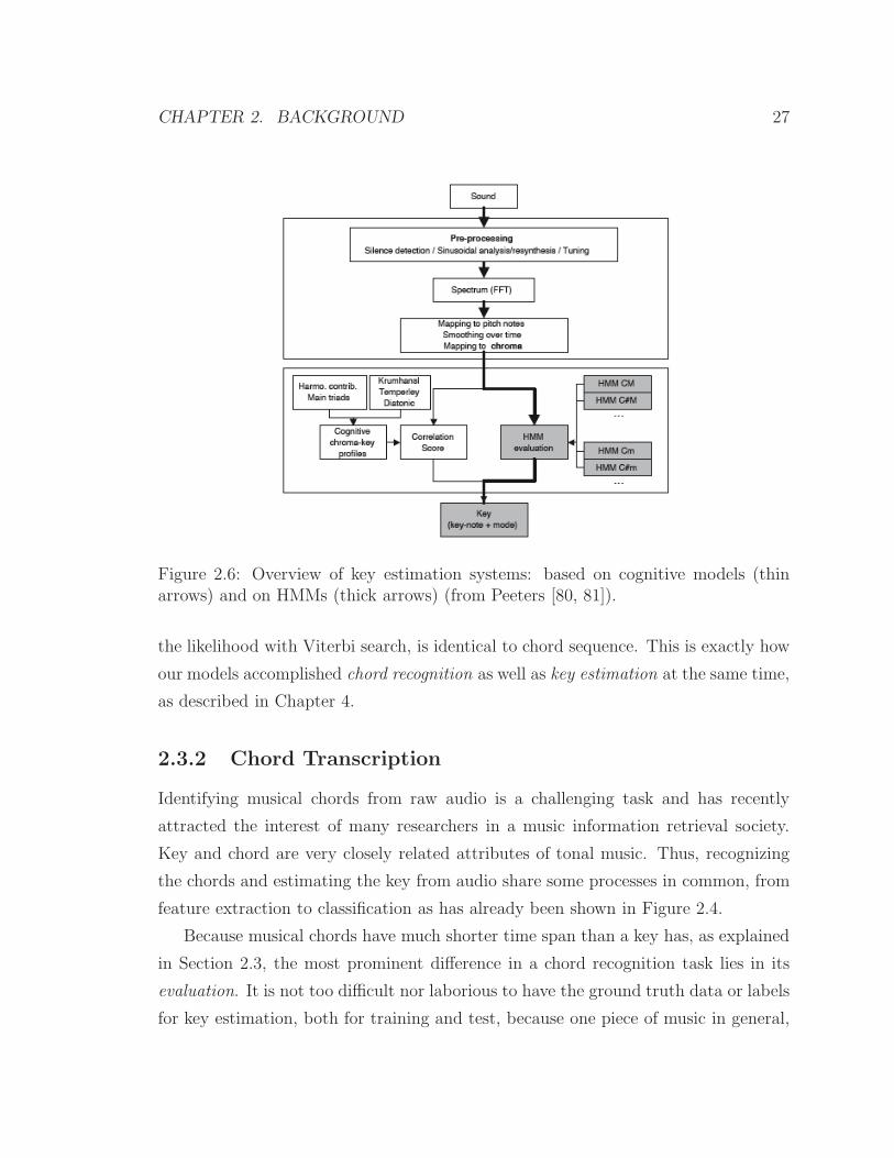
2.6 Overview of key estimation systems: based on cognitive models (thin
arrows) and on HMMs (thick arrows) (from Peeters [80, 81]). . . . . . 27
2.7 Flow diagram of the chord recognition system using a quantized chro-
magram (from Harte and Sandler [36]). . . . . . . . . . . . . . . . . . 30
2.8 State-transition distribution A: (a) initialization of A using the circle
of fifths, (b) trained on Another Crossroads (M. Chapman), (c) trained
on Eight days a week (The Beatles), and (d) trained on Love me do
(The Beatles). All axes represent the 24 lexical chords (C→B then
c→b). Adapted from Bello and Pickens [8]. . . . . . . . . . . . . . . . 33
xiv

2.9 Two-layer hierarchical representation of a musical chord (from Maddage
et al. [64]). . . . . . . . . . . . . . . . . . . . . . . . . . . . . . . . . 34
2.10 Overview of the automatic chord transcription system based on hy-
pothesis search (from Yoshioka et al. [101]). . . . . . . . . . . . . . . 35
2.11 Network structure of Kansei model (from Onishi et al. [75]). . . . . . 36
3.1 Two main stages in chord recognition systems. . . . . . . . . . . . . . 40
3.2 The pitch helix and chroma representation. Note Bn+1 is an octave
above note Bn (from Harte and Sandler [36]). . . . . . . . . . . . . . 43
3.3 12-bin chromagram of an excerpt from Bach’s Prelude in C major
performed by Glenn Gould. Each chroma vector is computed every
185 millisecond. . . . . . . . . . . . . . . . . . . . . . . . . . . . . . . 44
3.4 Computing the quantized chromagram (from Harte and Sandler [36]). 45
3.5 Tuning of Another Crossroads by Michael Chapman. (a) 36-bin chro-
magram (b) Peak distribution (c) Peak histogram and (d) 12-bin tuned
chromagram . . . . . . . . . . . . . . . . . . . . . . . . . . . . . . . . 46
3.6 The Harmonic Network or Tonnetz. Arrows show the three circularities
inherent in the network assuming enharmonic and octave equivalence
(from Harte et. al [37]). . . . . . . . . . . . . . . . . . . . . . . . . . 47
3.7 A projection showing how the 2-D Tonnetz wraps around the surface
of a 3-D Hypertorus. Spiral of fifths with pitch classes is shown as a
helical line (from Harte et. al [37]). . . . . . . . . . . . . . . . . . . . 47
3.8 Visualizing the 6-D Tonal Space as three circles: fifths, minor thirds,
and major thirds from left to right. Numbers on the circles correspond
to pitch classes and represent nearest neighbors in each circle. Tonal
Centroid for A major triad (pitch class 9,1, and 4) is shown at point
A (from Harte et. al [37]). . . . . . . . . . . . . . . . . . . . . . . . . 48
3.9 Training the chord transcription system. Labels obtained through har-
mony analysis on symbolic music files and feature vectors extracted
from audio synthesized from the same symbolic data are used to train
HMMs. . . . . . . . . . . . . . . . . . . . . . . . . . . . . . . . . . . . 51
xv

3.10 Chord and key distribution of classical (left) and Beatles (right) train-
ing data. . . . . . . . . . . . . . . . . . . . . . . . . . . . . . . . . . . 53
3.11 36x36 transition probability matrices obtained from 765 pieces of clas-
sical music and from 158 pieces of Beatles’ music. For viewing purpose,
logarithm is taken of the original matrices. Axes are labeled in the or-
der of major, minor and diminished chords. The right third of these
matrices are mostly zero because these musical pieces are unlikely to
transition from a major or minor chord to a diminished chord, and
once in a diminished chord, the music is likely to transition to a major
or minor chord again. . . . . . . . . . . . . . . . . . . . . . . . . . . . 55
3.12 Transition probabilities from C major chord estimated from classical
and from Beatles’ data. The X axis is labeled in the order of major,
minor and diminished chords. . . . . . . . . . . . . . . . . . . . . . . 56
3.13 Mean chroma vector and covariances for C major chord estimated from
classical and from Beatles’ data. Because we use diagonal covariance,
the variances are shown with “error” bars on each dimension. . . . . . 57
3.14 Mean tonal centroid vector and covariances for C major chord esti-
mated from classical and from Beatles’ data. Because we use diagonal
covariance, the variances are shown with “error” bars on each dimension. 58
3.15 Cross-evaluation between data-based and knowledge-based model. . . 59
3.16 Frame-rate recognition results for Bach’s Prelude in C Major performed
by Glenn Gould. Below 12-bin chromagram are the ground truth and
the recognition result using a C major key HMM trained on classical
symbolic music. . . . . . . . . . . . . . . . . . . . . . . . . . . . . . . 60
4.1 System for key estimation and chord recognition using key-dependent
models (K = 24). . . . . . . . . . . . . . . . . . . . . . . . . . . . . . 67
4.2 Key distribution of the training data (classical and the Beatles). . . . 68
xvi

4.3 Transition probabilities from a C major chord in C major key and in C
minor key HMM from classical data. The X axis is labeled in the order
of major, minor and diminished chords. Compare this to the generic
model shown in Figure 3.12. . . . . . . . . . . . . . . . . . . . . . . . 69
4.4 Comparison of a generic model with a key-dependent model. Model
numbers on the x-axis denote: 1) chroma, trained on Beatles; 2) tonal
centroid, trained on Beatles; 3) chroma, trained on classical; 4) tonal
centroid, trained on classical. . . . . . . . . . . . . . . . . . . . . . . 71
4.5 Frame-rate recognition results from Beatles’ Eight Days A Week. In
circles are the results of D major key model and in x’s are those of uni-
versal, key-independent model. Ground-truth labels and boundaries
are also shown. . . . . . . . . . . . . . . . . . . . . . . . . . . . . . . 72
4.6 Chord recognition system using genre-specific HMMs (G = 6). . . . . 74
4.7 36×36 transition probability matrices of rock (left), jazz (center), and
blues (right) model. For viewing purpose, logarithm was taken of the
original matrices. Axes are labeled in the order of major, minor, and
diminished chords. . . . . . . . . . . . . . . . . . . . . . . . . . . . . 76
4.8 Mean tonal centroid vectors and variances of C major chord in key-
board, chamber, and orchestral model. . . . . . . . . . . . . . . . . . 77
4.9 Chord recognition performance of a 36-state universal model with the
number of mixtures as a variable (solid) overlaid with a 24-state rock
model with one mixture (dash-dot). . . . . . . . . . . . . . . . . . . . 79
6.1 Overview of the coversong identification system. . . . . . . . . . . . . 90
6.2 Similarity matrix and minimum alignment cost of (a) cover pair and
(b) non-cover pair. . . . . . . . . . . . . . . . . . . . . . . . . . . . . 93
6.3 Averaged recall-precision graph. . . . . . . . . . . . . . . . . . . . . . 94
6.4 Self-similarity matrix of the first seconds from Bach’s Prelude No. 1
in C major performed by Gould (from Foote [28]). . . . . . . . . . . . 98
xvii

6.5 In dynamic programming, clustering in feature-space is done by finding
the optimal state-path based on a transition cost and a local cost. The
dotted diagonal is the nominal feature path. A candidate cluster path
is shown in solid line (from Goodwin and Laroche [35]). . . . . . . . . 100
6.6 The overview of structural segmentation system . . . . . . . . . . . . 102
6.7 Frame-level chord recognition results (The Beatles’ “No Reply”). . . . 104
6.8 Normalized autocorrelation of an impulse train obtained from the chord
sequence shown in Figure 6.7. . . . . . . . . . . . . . . . . . . . . . . 104
6.9 24 × 24 distance matrix between 12 major/minor chords in tonal cen-
troid space. Related chords are indicated by off-diagonals in lighter
colors (e.g. C-F, C-G, C-Cm, C-Am). . . . . . . . . . . . . . . . . . . 105
6.10 Tonal tension curve overlaid with the chord sequence (The Beatles’
“No Reply”). . . . . . . . . . . . . . . . . . . . . . . . . . . . . . . . 107
6.11 Final segmentation result. Estimated boundaries are shown in vertical
solid lines and true boundaries in dashed-dot lines (The Beatles’ “No
Reply”). . . . . . . . . . . . . . . . . . . . . . . . . . . . . . . . . . . 108
6.12 Distance matrix between segment pairs (The Beatles’ “No Reply”). . 109
6.13 Structural analysis: segmentation, clustering and summarization. . . 110
A.1 A Markov chain with 4 states (labeled S1 to S4) with all possible state
transitions. . . . . . . . . . . . . . . . . . . . . . . . . . . . . . . . . 125
A.2 An N -state urn and ball model of a discrete symbol HMM (adapted
from Rabiner [86]). . . . . . . . . . . . . . . . . . . . . . . . . . . . . 127
xviii

Chapter 1
Introduction
This dissertation discusses automatically extracting harmonic content — musical key
and chords — from the raw audio waveform. This work proposes a novel approach
that performs simultaneously two tasks — i.e., chord recognition and key estimation
— from real recordings using a machine learning model trained on synthesized audio.
This work also demonstrates several potential applications that use as a front end
harmonic descriptions derived from the system. This chapter serves as an introduc-
tion presenting the fundamental ideas on which this thesis was based and written,
which include the current research efforts in the field of music information retrieval,
the motivation and goals of this work, potential applications, and how this thesis is
organized.
1.1 Music Information Retrieval
Information retrieval (IR) is a field of science that deals with the representation, stor-
age, organization of, and access to information items [2]. Likewise, music information
retrieval (MIR) deals with the representation, storage, organization of, and access to
music information items. This is best described with an example by Downie [21]:
Imagine a world where you walk up to a computer and sing the
song fragment that has been plaguing you since breakfast. The
1
CHAPTER 1. INTRODUCTION 2
computer accepts your off-key singing, corrects your request, and
promptly suggests to you that “Camptown Races” is the cause of
your irritation. You confirm the computer’s suggestion by listen-
ing to one of the many MP3 files it has found. Satisfied, you
kindly decline the offer to retrieve all extant versions of the song,
including a recently released Italian rap rendition and an orches-
tral score featuring a bagpipe duet.
Music information retrieval is an interdisciplinary science, whose disciplines in-
clude information science, library science, computer science, electrical and computer
engineering, musicology, music theory, psychology, cognitive science, to name a few.
The problems in MIR are also multifaceted, due to the intricacies inherent in the
representation of music information. Downie defines seven facets which play a variety
of roles in defining the MIR domain — pitch, temporal, harmonic, timbral, editorial,
textual, and bibliographic facets [21]. These facets are not mutually exclusive but
interact with each other, making the problems more perplexing.
Finding more efficient and effective ways to search and retrieve music is attracting
increasing number of researchers both from academia and industries as it becomes
possible to have thousands of audio files in a hand-held device such as portable music
players or even in cellular phones. Furthermore, the distribution of music is also
changing from offline to online: more and more people are now buying music from
the web1, where more than tens of millions of songs are available. Therefore, users
need to manage and organize their large collection of music in a more sophisticated
way, and the content providers need to provide the users with an efficient way to find
music they want.
1.2 Motivation
People have been using the meta-data, almost exclusively, as a front end to search,
retrieve and organize through a large collection of music in their computer or on the
1As of 2/23/2006, more than 1,000,000,000 songs were downloaded from iTunes only,which is an online music store by Apple Computer [67].

CHAPTER 1. INTRODUCTION 3
Internet. Meta-data, sometimes called tags, are textual representations that describe
data, to facilitate the understanding, organization and management. In the music do-
main, meta-data may include the title of a piece, the name of an artist or a composer,
the name of a performer, or the musical genre. An example is “Eight Days A Week
(song title)” by “Beatles (artist, composer)”, which belongs to “rock (genre)” music.
Another example is “Piano Sonata No. 14 in C♯ minor, Op. 27 (title)” by “Beethoven
(composer)”, performed by “Glenn Gould (performer),” which is “classical (genre)”
music.
These textual descriptions of music are very compact and therefore extremely
efficient for search and retrieval, especially when there are a great number of items
to be searched. However, the textual meta-data is far from being ideal in many
situations. First of all, their usage is limited in that all the required information must
be previously prepared — i.e., someone has to manually enter the corresponding
information — or the search is bound to fail. This is likely to happen especially
when new songs are released.2 Second, the user must know exactly what the query
is, which might not be always the case: he/she might not be able to recall the name
of a song or an artist. Third, they might not be as effective in particular tasks. For
instance, imagine a situation where a user wants to find musically similar songs to
his/her favorite ones using the meta-data only. Chances are the returned items may
not be similar at all because there is very little correspondence between the distance
in a meta-data space and the distance in a musical space.
It is not too difficult to infer the cause of the problems described above: a piece
of music is a whole entity, and music listening is an experience that requires a set of
hierarchical processes from low-level, auditory perception to high-level cognition, of-
ten including emotional processes. Therefore, it is almost impossible to fully describe
music with just a few words, although they may convey important and/or relevant
information about music. Meta-data may help us guess what it’s like but we can
truly comprehend the actual content only through listening experiences. This is why
content-based approaches in MIR attract researchers from diverse disciplines.
210,000 new albums are released and 100,000 works registered for copyright every yearas of 1999 [97].

CHAPTER 1. INTRODUCTION 4
1.2.1 Content-based Approach
Recently, due to limitations and problems of the meta-data-driven approaches in mu-
sic information retrieval, a number of researchers are actively working on developing
systems based on content description of musical audio. Cambridge Online Dictionary
defines the word content as: the ideas that are contained in a piece of writing, a
speech or a film.3 Therefore, instead of describing music with only a few words such
as its title, composer, or artist, content-based methods try to find more meaningful
information implicitly conveyed in a piece of music by analyzing the audio itself.
It is nearly impossible to figure out from the raw audio the high-level ideas that the
composers tried to express via musical pieces. However, music is not written based on
random processes. There are rules and attributes in music to which most composers
conform when writing their music. This is especially true in Western tonal music.
Therefore, if we can extract these musical rules and/or attributes from audio that
the composers used in writing music, it is possible to correlate them with higher-level
semantic description of music — i.e., the ideas, thoughts or even emotional states
which the composers had in mind and tried to reflect through music they wrote. We
are not trying to say that the conventional meta-data like song title or genre are
useless; they are very useful and efficient in some tasks. However, these high-level
semantic descriptions obtained through content analysis give information far more
relevant to music itself, which can be obtained only through listening experience.
There are several attributes in Western tonal music, including melody, harmony,
key, rhythm or tempo. Each of these attributes has its unique role, and yet still
interacts with the others in a very controlled and sophisticated way. In the next
section, we explain why we believe harmony and key, among many attributes, are
particularly important in representing musical audio signals of tonal music where the
tonal organization is primarily diatonic.
3http://dictionary.cambridge.org
CHAPTER 1. INTRODUCTION 5
1.2.2 Harmonic Description of Tonal Music
Harmony is one of the most important attributes of Western tonal music. The im-
portance of harmony in tonal music is emphasized by a number of treatises written
over the centuries. Ratner explains harmony in three different and yet closely related
contexts: harmonic sonorities, harmonic action and harmonic color [88].
Harmonic sonorities are about the stability/instability embodied in a set of simul-
taneously sounding notes (intervals, chords) and their contributions to the sense of
a key and to musical movement and arrival. Mutual relationships of tones and their
qualities and effects expressed by various intervals and chords constitute the basis of
harmony in Western tonal music.
Changes over time in these harmonic relationships — intervals, the sense of key,
stability/instability, chords — ensure the power, or harmonic action, to carry musical
movement forward. Like all action, harmonic action proceeds through a cycle of
departure, movement and arrival. Among a number of characteristic patterns and
formulas that realize this cycle, including melodic elaboration, rhythmic patterns of
chord change, voice leading and modulation, the cadential formula is by far the most
important. Two basic aspects of harmony embodied in the cadential formula — i.e.,
the movement-instability and the arrival-stability represented by the tritone4 and the
tonal center, respectively — create a clear sense of key, from which a small segment
of musical structure has taken.
While it was the most important role of harmony to create the organic, structurally
firm embodiment of key in the eighteenth century and in the early nineteenth century,
the element of color in harmony was exploited and became increasingly important as
composers sought to develop and enrich their sounds and textures, especially in the
late nineteenth century and in the twentieth century.
Among the three aspects of harmony described above, the description of harmonic
action in particular clearly suggests that we can infer a musical structure from har-
mony by detecting changes in local key or by finding the cadential formula. Further-
more, because a strong sense of key is created by some specific harmonic movement
4A tritone is also called an augmented fourth and is an interval that is composed of threewhole tones, e.g., C-F♯.
CHAPTER 1. INTRODUCTION 6
or the cadential formula, it shouldn’t be difficult to infer a key once we figure out
how harmony progresses over time.
Other than analyzing the structure of music, harmonic description of tonal music
can be used as an efficient, robust front end in practical applications. For example,
when finding different versions of the same song (or so-called cover songs), harmonic
content remains largely preserved under severe acoustical variations due to changes
in tempo, dynamics and/or instrumentation, and therefore it can be a robust front
end in such application. Another potential application is recommendation or playlist
generation; i.e., use harmonic content to compute (dis)similarity between songs and
recommend only those that are harmonically similar to the user’s existing collection
of music.
1.2.3 Machine Learning in Music Applications
Machine learning is the study of computer algorithms that improve automatically
through experience [68]. There are a number of real-world applications that benefit
greatly from the machine learning techniques, including data mining, speech recogni-
tion, hand-writing recognition, and computer vision, to name a few. In MIR, many
systems also use machine learning algorithms to solve problems such as genre classi-
fication [96, 4, 5], instrument identification [99, 24] and key estimation [14, 73].
Speech recognition is one of many application areas for which machine learning
methods have made significant contributions. Research for the last 20 years shows
that among many machine learning models, HMMs are very successful for speech
recognition. A hidden Markov model [86] is an extension of a discrete Markov model,
in which the states are hidden in the sense that we can not directly observe the
underlying stochastic process, but can only observe it through another set of stochastic
processes. The more details about the HMMs are found in Appendix A.
Much progress in speech recognition has been made with gigantic databases of
labeled speech. Such a huge database not only enables researchers to build richer
models, but also allows them to estimate the model parameters precisely, resulting
in improved performance. However, there are very few such databases available for
CHAPTER 1. INTRODUCTION 7
music. Furthermore, the acoustical variance in music is far greater than that in speech,
in terms of its frequency range, timbre due to different instrumentations, dynamics
and/or duration. Consider the huge acoustical differences among: a C major chord
in root position played by a piano, the same chord in first inversion played by a rock
band, and the same chord in second inversion played by a full orchestra. All of these
sounds must be transcribed as the same C major chord; this in turn means even more
data are needed to train the models so they generalize.5
However, it is very difficult to obtain a large set of training data for music, par-
ticularly for chord recognition. First of all, acquiring a large collection of music is
expensive. In addition, in order to obtain the ground-truth annotation, we need a
certain level of expertise in music theory or musicology to perform harmony analy-
sis. Furthermore, hand-labeling the chord boundaries in a number of recordings is
not only an extremely time consuming and tedious task, but also is subject to errors
made by humans. In the next section, we describe how we solve this bottleneck prob-
lem of acquiring a large amount of training data with minimal human labor by using
symbolic music documents.
1.2.4 Symbolic Music Documents
In this dissertation, we propose a method of automating the daunting task of pro-
viding the machine-learning models with labeled training data. To this end, we use
symbolic music documents, such as MIDI files, to generate chord names and precise
corresponding boundaries, as well as to create audio. Instead of a digitized audio
signal like a PCM waveform, MIDI files contain a set of event messages such as pitch,
velocity and note duration, along with clock signals from which we can synthesize
audio. Audio and chord-boundary information generated this way are in perfect
alignment, and we can use them to directly estimate the model parameters. The
overall process of training is illustrated in Figure 3.9.
The rationale behind the idea of using symbolic music files for automatic harmony
5A model is called generalized when it performs equally well on various kinds of inputs.On the other hand, it is called overfitted if it performs well only on a particular input.

CHAPTER 1. INTRODUCTION 8
time: 0 1.5 3.2 6.0 ...
(MIDI)
(.lab)
Label
MIDI synthesis
Audio
(.wav)
HMMs
Training
Feature vectors
Key
chord name: C G D7 Em ...
Harmonic analysis
Symbolic data
Feature extraction
Figure 1.1: Training the chord transcription system. Labels obtained through har-mony analysis on symbolic music files and feature vectors extracted from audio syn-thesized from the same symbolic data are used to train HMMs.
CHAPTER 1. INTRODUCTION 9
analysis is that they contain noise-free pitch and on/offset time information of ev-
ery single note, from which musical chords are transcribed with more accuracy and
easiness than from real acoustic recordings. In addition, other information included
in symbolic music files, such as key, allow us to build richer models, like key-specific
models.
There are several advantages to this approach. First, a great number of symbolic
music files are freely available. Second, we do not need to manually annotate chord
boundaries with chord names to obtain training data. Third, we can generate as much
data as needed with the same symbolic files but with different musical attributes by
changing instrumentation, tempo or dynamics when synthesizing audio. This helps
avoid overfitting the models to a specific type of sound. Fourth, sufficient training
data enables us to build richer models so that we can include more chord types
such as a 7th, augmented or diminished. Lastly, by using a sample-based synthesis
technique, we can generate harmonically rich audio as in real acoustic recordings.
Although there may be noticeable differences in sonic quality between real acoustic
recording and synthesized audio, we do not believe that the lack of human touch,
which makes a typical MIDI performance dry, affects our training program. The fact
that our models trained on synthesized audio perform very well on real recordings
supports this hypothesis. In the next section we present the goals of the current work.
1.3 Goals
We present here the goals of this dissertation work.
1. Review and analyze related work on chord transcription and key finding. Present
not only technical perspectives such as audio signal processing and machine
learning algorithms, but also music theoretical/cognitive studies, which provide
fundamental background to current work.
2. Describe the system in complete detail, which includes: 1) feature extraction
from the raw audio; 2) building and training of the machine learning-models;

CHAPTER 1. INTRODUCTION 10
3) recognition of chords and key from an unknown input; 4) and the further
extensions of the models.
3. Provide quantitative evaluation methods to measure the performance of the
system.
4. Perform thorough analysis of the experimental results and prove the state-of-
the-art performance, including robustness of our system using various types of
test audio.
5. Validate our main hypothesis — i.e., harmony is a very compact and robust mid-
level representation of musical audio — by using it as a front end to practical
applications.
6. Discuss the strength and weakness of the system and suggest the directions for
improvement.
In the next section, we describe several potential applications in which we use
harmonic content automatically extracted from audio.
1.4 Potential Applications
As aforementioned in Section 1.2.2, in Western tonal music, once we know musical
key and chord progression of a piece over time, it is possible to perform structural
analysis from which we can define themes, phrases or forms. Although other musical
properties like melody or rhythm are not irrelevant, harmonic progression has the
closest relationships with the musical structure. Finding structural boundaries in
musical audio is often referred to as structural music segmentation.
Once we find the structural boundaries, we can also group similar segments into a
cluster, such as a verse or chorus in popular music, by computing the (dis)similarity
between the segments. Then it is also possible to do music summarization by
finding the most repetitive segment, which in general is the most representative part
in most popular music.

CHAPTER 1. INTRODUCTION 11
A sequence of chords and the timing of chord boundaries are also a compact and
robust mid-level representation of musical signals that can be used to find the cover
version(s) of the original recording, or cover song identification, as shown by Lee
[56] and by Bello [7]. Another similar application where chord sequence might be
useful is music similarity finding because a original-cover pair is an extreme case
of similar music.
We describe these applications in more detail and demonstrate the possibilities of
our approach with real-world examples in Chapter 6.
1.5 Organization
This dissertation continues with a scientific background in Chapter 2, where related
works are reviewed. In Chapter 3, we fully describe our chord recognition system,
including the feature set we use as a front end to the system, and the method of
obtaining the labeled training data. We also describe the procedure of building the
model, and present the experimental results. In Chapter 4, we propose the method
of extending our chord recognition model to key or genre-specific models to estimate
key or genre as well as to improve the chord recognition performance. In Chapter 5,
we present a more advanced model — discriminative HMMs — that uses a powerful
discriminative algorithm to compute the posterior distributions. In Chapter 6, we
demonstrate that we can use the chord sequence as a front end in applications such as
audio cover song identification, structural segmentation/clustering of musical audio,
and music summarization. Finally, in Chapter 7, we summarize our work and draw
conclusions, followed by directions for future work.

Chapter 2
Background
2.1 Introduction
In this chapter, we review previous research efforts on key extraction and chord recog-
nition, and on tonal description of musical audio, which are very closely related with
each other. In doing so, we first present related studies from the perspective of music
theory and cognition that serve as fundamental background to most computational
algorithms, including ours.
2.2 Tonality
Hyer explains the term tonality as:
A term first used by Choron in 1810 to describe the arrangement
of the dominant and subdominant above and below the tonic and
thus to differentiate the harmonic organization of modern mu-
sic (tonalite moderne) from that of earlier music (tonalite an-
tique). One of the main conceptual categories in Western musical
thought, the term most often refers to the orientation of melodies
and harmonies towards a referential (or tonic) pitch class. In the
12
CHAPTER 2. BACKGROUND 13
broadest possible sense, however, it refers to systematic arrange-
ments of pitch phenomena and relations between them [40].
According to Hyer, there are two main historical traditions of theoretical concep-
tualization about tonal music: the function theories of Rameau and Riemann on the
one hand and the scale-degree theories of Gottfried Weber and Schenker on the other.
The first tradition corresponds to the definition of tonality by Choron and the second
corresponds to that by Fetis, who places more emphasis on the order and the position
of pitches within a scale. However, in both traditions, tonal theories tend to concen-
trate on harmonic matter, virtually excluding all other musical phenomena such as
register, texture, instrumentation, dynamics etc. These features are considered only
to the extent that they articulate or bring out relations between harmonies.
We can describe tonality using two musical properties — key and harmony. A
key is a tonal center or a referential point upon which other musical phenomena such
as melody or harmony are arranged. Ratner states that the key is a comprehensive
and logical plan coordinated from the interplay of harmonic stability and instability
of intervals, which leads to a practical working relationship between tones [88]. There
are two basic modes in the key: major and minor mode. Therefore, key and mode
together define the relative spacing between pitch classes, centered on a specific pitch
class (tonic). When the two keys share the same tonal center (such as in C major and
C minor key), they have parallel major-minor relationship. On the other hand, if a
sequence of notes in the two keys have the same relative spacing but have different
tonal centers (such as in C major and A minor key), we refer to them as relative keys.
If a key is a tonal center that functions as a point of departure, reference en route
and arrival, it is harmony that carries musical movement forward and at the same
time control and focus movement [88]. A phase of harmonic movement or action
is created through a cycle of departure, movement and arrival, and each point of
arrival becomes in turn a new point of departure. This series of phases of harmonic
movement shape musical structure. Among many rules and patterns in realizing a
phase of harmonic movement, the cadential formula is the most important one. The
cadence or cadential formula is defined as:

CHAPTER 2. BACKGROUND 14
The conclusion to a phrase, movement or piece based on a rec-
ognizable melodic formula, harmonic progression or dissonance
resolution; the formula on which such a conclusion is based. The
cadence is the most effective way of establishing or affirming the
tonality — or, in its broadest sense, modality — of an entire
work or the smallest section thereof; it may be said to contain the
essence of the melodic (including rhythmic) and harmonic move-
ment, hence of the musical language, that characterizes the style
to which it belongs [89].
As is defined above, a cadence concludes a phrase or movement and is recognized
by a specific harmonic progression or melodic formula. Therefore, if we know key and
harmonic progression in tonal music, then we can identify cadences which indicate
phrase boundaries.
2.2.1 Perception/Cognition of Tonality
The scope of the current dissertation is bounded by recognition of chords/key of simple
diatonic music like pop or rock music. Furthermore, it does not include any sort of
music cognitive or music theoretical experiments/studies, which cover more general
and a broader range of Western tonal music. However, many computer algorithms
make use of findings by such music cognitive/theoretical studies to infer tonality
in Western tonal music, and we believe that presenting some landmark studies in
perception/cognition of tonal music will help better understand the computer models
as well.
There are many approaches to understand and model how humans perceive tonal
music from the perspectives of cognitive science and psychology. We describe some of
them here, but interested readers are advised to see Gomez [32] for a more complete
summary.
Krumhansl and her colleagues did extensive research to investigate and model the
relationship between musical attributes that are perceived and psychological experi-
ences corresponding musical attributes through empirical studies [49, 50, 52].

CHAPTER 2. BACKGROUND 15
Krumhansl and Shepard introduced the probe tone method to quantify the hi-
erarchy of stability within a major key context [52]. In this study, they observed
that when an “incomplete” scale is sounded, such as the successive tones C, D, E, F,
G, A, B, this creates strong expectations about the tone that is to follow. In their
experiments, they presented to the subjects two sequence of notes in a C major scale
— the ascending scale of C, D, E, F, G, A, B and the descending scale of C, B, A,
G, F, E, D — followed by the probe tone. The task of the subjects was to rate the
degree of how well the given probe tone completes a sequence of notes from 1 (very
bad) to 7 (very good). The probe tones were the equal-tempered semitones in the
chromatic scale ranging from middle C to the C an octave above (thus the 13 probe
tones total). From the results of the experiments, they found three distinct patterns
depending on the level of prior musical experience.
Based on the initial study, Krumhansl and Kessler extended their experiments to
minor-key contexts, resulting in two probe tone ratings, one for each key context [50].
Figure 2.1 shows the key profiles for a major and a minor key obtained from these
probetone ratings.
Using these key-profiles obtained from the probe-tone experiments, they calculated
the key-distances between the two arbitrary keys following the steps: 1) perform
circulative permutation on the two key-profiles (major and minor) to obtain 12 major
and 12 minor key-profiles, one for each pitch class; 2) compute correlations between
a pair of key-profiles for every possible pair. Figure 2.2 shows correlations between
a C major key-profile and all other major and minor key-profiles, and correlations
between a C minor key-profile and all other major and minor key-profiles.
They further extended their studies to investigate how the relation between a
chord and its abstract tonal center, or key, may be represented in a two-dimensional
map of the multidimensional scaling solution of the 24 major and minor keys. Figure
2.3 illustrates how the C major, A minor, and B diminished chords appear in the
spatial map of musical keys.
Krumhansl proposed a key-finding algorithm using the key-profiles and the max-
imum correlation analysis. She first computed the input vector I = d1, d2, · · · , d12,

CHAPTER 2. BACKGROUND 16
Figure 2.1: C major and C minor key-profiles obtained from the probe tone ratingexperiments (from Krumhansl and Kessler [50]).
each dimension representing the tone duration in musical selection. She then com-
puted correlations between the input vector I and the probe tone profiles Ki, k =
1, 2, · · · , 24 for 24 keys. The output is a 24-dimensional vector, where each element
represents correlation between the input vector and each key. Using the 48 fugues of
Bach’s, Krumhansl and Schmuckler showed that their algorithm needs fewer number
of tones to find the correct key [51].
A series of studies and experiments done by Krumhansl and her collaborators
made significant contributions to understanding how listeners encode, organize, and

CHAPTER 2. BACKGROUND 17
C Db D Eb E F Gb G Ab A Bb B−1
−0.5
0
0.5
1C
orrle
atio
n
C C# D Eb E F F# G G# A Bb B−1
−0.5
0
0.5
1
C major
C Db D Eb E F Gb G Ab A Bb B−1
−0.5
0
0.5
1
MajorC C# D Eb E F F# G G# A Bb B
−1
−0.5
0
0.5
1
C minor
Minor
Figure 2.2: Correlations between C major and all other key-profiles (top) and correla-tions between C minor and all other key-profiles (bottom) calculated from the probetone ratings by Krumhansl and Kessler [50].
remember pitch patterns in music. Furthermore, although they approached the prob-
lems from the perspectives of cognitive science and psychology, they had a giant
impact on a number of computer algorithms that try to infer tonality from music,
both from symbolic music and from musical audio.
In the next section, we review computer systems that automatically identify mu-
sical key and/or chords from the real recordings.

CHAPTER 2. BACKGROUND 18
Figure 2.3: The relations between the C major, A minor and B diminished chords andthe 24 keys displayed in a 2-dimensional map of keys (from Krumhansl and Kessler[50]).
CHAPTER 2. BACKGROUND 19
2.3 Computer Systems
In Western tonal music, key and chord are two closely-related attributes, as mentioned
above. Musical key defines a set of rules that harmony, as well as melody, abide by
in the course of musical development. Therefore, if a piece of Western tonal music is
in a certain key, we can predict not only the kind of chords that are most likely to
appear but also how they are going to progress over time. Conversely, analyzing the
chords and their pattern of progression also suggests key information.
Because musical key and chords have such close relatioships, computer systems for
key estimation and those for chord recognition are also alike. The biggest difference
lies in the scope of temporal dynamics — key is more a global attribute while chords
are much more local. That is, while key seldom changes (or never for many popular
music), chords changes even more frequently. This difference in temporal dynamics
has a great impact on building systems, particularly in machine learning approaches,
because it is much more difficult to obtain the training data for chord recognition
systems.
Most algorithms for key-finding and chord recognition from audio are divided into
two main stages: feature extraction and classification, as illustrated in Figure 2.4. In
the feature extraction stage, the computer system extracts appropriate feature vectors
from the raw audio because raw audio samples are redundant and not robust. The
feature vectors must satisfy the following conditions. First, the feature must be low
in dimension or the system will be computationally expensive. This is unacceptable
for real-time applications. Furthermore, high dimensionality is likely to cause a data
sparsity problem in statistical classifiers.
Second, the feature must be robust to the kinds of acoustical variations present
in music. That is to say, it must remain largely invariant no matter how the musical
acoustics vary unless the key or chord should change. For example, the features from
Bach’s Prelude in C major and The Beatles’ No Reply, which is also in the key of
C major, should be closer to each other in distance than to other keys. A similar
argument holds for chord recognition as well. Once suitable features are extracted
from the raw audio, the classification algorithms classify the given feature to the

CHAPTER 2. BACKGROUND 20
Key (Chord)
Feature
Extraction
Audio
Feature vector
Classifier
Tonal CentroidChroma
HMM
Template Matching
Tuning DetectionCQTFFT
Figure 2.4: General overview of key estimation and chord recognition system.
correct chord or key.
While there is an almost unanimous agreement in the choice of the feature for
both key estimation and chord recognition, the classifiers are mainly divided into two
groups: some use a simple pattern matching algorithm based on pre-defined key or
chord templates, and others depend on more complex, sophisticated statistical learn-
ing algorithms. Therefore, in the following two sections, we sub-divide systems for
each task into two categories — template matching algorithms and machine learning
algorithms — and describe each algorithm in more detail.
CHAPTER 2. BACKGROUND 21
2.3.1 Key Estimation
Template Matching Approaches
Template matching techniques for key estimation use pre-defined key templates (e.g.,
Krumhansl’s key-profiles) for each key, and correlate them with the feature vector
computed from audio to find the key template that yields the maximum correlation
coefficient.
Pauws proposed a key extraction algorithm from audio based on human auditory
perception and music cognition, and evaluated his algorithm using 237 classical piano
sonatas [79]. He first computed a non-overlapping chromagram1 over six octaves from
A0 to A6 (27.5 Hz to 1760 Hz), and used it as input to the maximum-key profile corre-
lation (MKC) algorithm to estimate musical key. Chroma vector is a 12-dimensional
vector, each dimension representing the spectral energy in a chromatic scale. Because
it is not only based on the actual musical scale (i.e., equal-tempered scale2), but also
because of its computational efficiency and low dimensionality, chroma feature is a
common choice for key extraction and/or chord recognition.
In computing a chromagram, however, he went through several pre-processing
stages to obtain the harmonically compressed spectrum, including low-pass filtering,
enhancing spectral components to cancel out spurious peaks, logarithmic frequency
scaling, and the use of weighting function to model the human auditory sensitiv-
ity. After adding and normalizing the chromagrams over all frames, he applied the
maximum-key profile correlation (MKC) algorithm based on key profiles derived by
Krumhansl and Kessler [50]. The key profile yielding the maximum correlation value
out of 24 possible keys was recognized as the key of input musical audio. Using
237 classical piano sonatas as test data, his algorithm gave an accuracy of 75.1% by
counting only exact matches as correct. Including related keys — relative, dominant,
sub-dominant and parallel — as correct matches, the accuracy went up to 94.1%.
Based on the observation that the scale root note plays the foremost role in tonal
1A chromagram is a two-dimensional representation of chroma vectors, similar to a spec-trogram.
2In the 12-tone equal-tempered scale, an octave is divided into 12 logarithmically equalsteps.

CHAPTER 2. BACKGROUND 22
Figure 2.5: Diagram of key detection method (from Zhu et al. [102]).
music, Zhu et al. proposed an approach to detect the scale root and the key from
audio [102]. They first extracted the pitch profile feature, similar to the chroma
feature, which characterizes the probability of the presence of particular tones in the
audio signal. In doing so, they performed four steps: (1) constant-Q transform of
the signal (CQT) to represent the signal in frequency domain; (2) the tuning pitch is
determined to correct mis-tuning of the music signal; (3) note partials are extracted
based on the energy of the CQT spectrum; (4) with the extracted note partial tracks, a
pitch profile feature is generated by a consonance filtering and pitch profiling process.
An overview of the system is shown in Figure 2.5.
A novel part of their algorithm is the key detection stage. From the pitch profile
feature generated using the processes described above, they first estimated the root
of the diatonic scale, whose structure they argued is much more salient and robust
than the structure of the key. They then conducted the key detection using both
the pitch profile feature and the estimated diatonic scale root. Using 60 pieces of
pop music and 12 pieces of classical music, the accuracy they obtained was 90% and
83.3%, respectively, arguing most errors were due to key modulation.
Most errors in these key-finding algorithms come from the confusion between
closely-related keys such as relative, dominant, sub-dominant or parallel. After careful

CHAPTER 2. BACKGROUND 23
examination of the source of most errors, Chuan and Chew proposed a fuzzy analysis
technique to extract more correct pitch classes, which improves the accuracy of key
finding [16, 17]. They also found that the source of this confusion was caused by noisy
detection of lower pitches, and by the biased raw frequency data.
Chuan and Chew’s fuzzy analysis technique to clarify pitch information from the
FFT has three steps: 1) clarify membership in the lower frequency range using knowl-
edge of the overtone series; 2) scale the FFT in pre-defined range to acknowledge the
presence of important pitches, or so called adaptive level weighting ; 3) refine pitch class
distribution by setting all normalized pitch class values 0.2 and below to zero, and 0.8
and above to one. They then applied Spiral Array Center of Effect Generator (CEG)
algorithm to determine the key. In the CEG algorithm, the key selection is done by a
nearest neighbor search in the Spiral Array space, which is a three-dimensional helical
representation of pitch relations [15].
Their evaluation with 410 classical music pieces shows an increase in accuracy
with their fuzzy analysis technique compared to a simple peak detection technique,
achieving a maximum correct rate of 75.25%. The test audio was all synthesized from
the MIDI files, and thus they failed to provide the results with real recordings.
While the previous algorithms used pre-defined key-profiles against which the
extracted feature was correlated, Van de Par et al. [98] used chromagrams extracted
from a collection of musical audio to train three key profiles for major and another
three for minor keys, respectively. The three trained key profiles are different in their
temporal weighting of information across the duration of each song. In other words,
one profile uses uniform weighing, another weighs more on the beginning, and the
third puts emphasis on the end of the song, respectively.
Once the key profiles have been trained, three chromagrams are extracted from
the test audio as well using the three temporal weighting functions. Each of these
extracted chromagrams is correlated with their respective key profiles, yielding three
correlation values that relate to the beginning, ending, and totality of the song.
Although an evaluation with the same database used by Pauws [79] (237 classical
piano pieces by Bach, Shostakovich, Brahms and Chopin) yields a very high rate of
98% correct classification, the test set was very small (2% or 5 pieces) compared with

CHAPTER 2. BACKGROUND 24
a large training data set (98% or 232 pieces). For a more reliable and complete test, a
k-fold cross validation with k = 10 or so would be more desirable. Furthermore, the
method of combining the results from the three different key profiles was empirical,
failing to provide logical grounds.
All key-finding algorithms described above find a single, global key from an entire
song, which is not true when there is key modulation. Furthermore, key modulation
is often the source of errors. Izmirli proposed a model for localized key finding from
audio using non-negative factorization for segmentation [76, 77]. He used the con-
ventional chroma vector as a feature. To compensate for possible mis-tuning present
in recordings, however, he applied an adaptive tuning algorithm before computing
a chromagram. He then performed non-negative factorization on the tuned chroma-
gram for segmentation based on tonal features to reveal the additive contributions of
tonal elements in a piece.
After segmenting the whole chromagram into sections with localized keys using
the NMF algorithm, he used a correlation method over the first segment to obtain the
global key of a piece. Using three different sets of test data (17 pop, 152 classical from
the Naxos set3 and 17 classical excerpts from Kostka and Payne [46]), he obtained
a performance of 87.0%, 84.1% and 97.1%, respectively for each test data set. His
algorithm also ranked first in the Audio Key Finding task in the MIREX 2005.4
Machine Learning Approaches
The key finding systems described so far use pre-defined key templates with which
the extracted feature from audio is correlated to find the closest key template. There-
fore, their performance is dependent on the choice of the templates, which are either
heuristically defined or based on the experimental data.
While these algorithms work fairly well, the pre-defined templates fail to represent
the actual organization of pitch classes in real music. Furthermore, it is very diffi-
cult to directly relate the low-level acoustical features such as chroma vector to the
3http://www.naxos.com4Music Information Retrieval Evaluation eXchange (http://www.music-ir.org/
mirexwiki/index.php/Main Page).

CHAPTER 2. BACKGROUND 25
high-level feature obtained from cognitive studies. Therefore, researchers turn their
attentions to alternative approaches, where they learn the rules that may define the
key from the actual musical audio.
Chai and Vercoe presented a hidden Markov model-based approach to detect the
segmental boundaries determined by key changes in musical audio, and identified the
key in each segment [14]. They used the 24-dimensional chromagram as a front end
instead of the conventional 12-dimensional one. Key detection is composed of two
sequential stages. First, they estimate the key without differentiating by mode. For
instance, C major and A minor key are regarded as the same key without considering
its mode. This results in only 12 different keys for each pitch class. Second, after the
key is identified, they determine the mode. This two-stage approach is based on the
assumptions that they use diatonic scales, and relative modes share the same diatonic
scale.
Chai and Vercoe then built hidden Markov models (HMMs) for each task: 12-state
HMMs for key detection and 2-state HMMs for mode detection. In estimating the
model parameters, i.e., the initial state distribution, the state transition probability
distribution and the observation probability distribution, they used empirical values
based on music-theoretical knowledge, instead of learning from the training data.
Using 10 pieces of classical piano music, Chai and Vercoe evaluated their system
with three different measures, including recall, precision and label accuracy, with
promising results. Instead of using a simple pattern-matching algorithm, they chose
to use a more sophisticated, statistical approach to detect the key modulation as
well as extract the key. However, their estimation of model parameters, which is
the most important step in all statistical learning models, was 100% heuristic and
therefore fails to make a full use of powerful machine-learning algorithms. This is
probably due to lack of sufficient training data, which is usually obtained through a
extremely laborious process of manual annotation, and again supports our method of
using symbolic music files to generate a large amount of training data for free.
While the abovementioned model is in part knowledge-based, i.e., the model pa-
rameters are initialized based on music-theoretical knowledge, Peeters proposed a
key-finding system that is purely data-based [81, 80]: that is, no prior knowledge is

CHAPTER 2. BACKGROUND 26
encoded and the model parameters are learned from the data only. The advantages of
a machine-learning approach are, he argues: 1) it does not make assumptions about
the presence of harmonics of the pitch notes in chroma vectors; 2) it does not require
the choice of a specific key-profile such as Krumhansl, Temperley or Diatonic, etc.; 3)
it allows possible key modulation over time through the transition probabilities. He
also used HMMs with chroma features as a front end, and compared his model with
the ones based on cognitive models
Based on the chroma feature vectors and corresponding key labels, Peeters built
24 HMMs, one for each key. Due to different number of instances for each key, he
first trained only two models, a major and a minor mode model, and mapped the two
trained models to the various other key-note models, resulting in 24 major/minor key
models. This mapping is performed by circular permutation of observation distribu-
tion parameters, i.e., mean vectors and covariance matrices. The final key estimation
is done by computing the likelihood of each key model given an unknown chroma
sequence, and selecting a model with the maximum likelihood. Figure 2.6 shows an
overview of his key estimation system.
A comparison with the cognitive models based on Krumhansl’s key-profiles using
302 classical music excerpts shows that his model is outperformed in several different
measures, although the difference in performance is not significant. Particularly, the
confusion with closely-related keys was larger than the one in the cognitive model-
based approach. Counting the related keys as correct matches, the accuracy between
the two models is similar (94.9% for HMMs and 95.0% for cognitive models).
Although Peeters’ data-driven approach achieves lower scores than the template-
matching methods based on cognitive models, it is noteworthy that no prior musical
knowledge was used in his model, proving that the system could successfully learn
the characteristics of keys from the data. In his models, he used three to nine hidden
states and the meaning of the state remains unspecified. This is because he is not
interested in decoding the state path, but only interested in finding the key model
giving the maximum likelihood. If the states had musical meanings, such as chords,
however, the results might have been better because musical keys and chords are very
closely related. In addition, the optimal state path, which comes free when computing
CHAPTER 2. BACKGROUND 27
Figure 2.6: Overview of key estimation systems: based on cognitive models (thinarrows) and on HMMs (thick arrows) (from Peeters [80, 81]).
the likelihood with Viterbi search, is identical to chord sequence. This is exactly how
our models accomplished chord recognition as well as key estimation at the same time,
as described in Chapter 4.
2.3.2 Chord Transcription
Identifying musical chords from raw audio is a challenging task and has recently
attracted the interest of many researchers in a music information retrieval society.
Key and chord are very closely related attributes of tonal music. Thus, recognizing
the chords and estimating the key from audio share some processes in common, from
feature extraction to classification as has already been shown in Figure 2.4.
Because musical chords have much shorter time span than a key has, as explained
in Section 2.3, the most prominent difference in a chord recognition task lies in its
evaluation. It is not too difficult nor laborious to have the ground truth data or labels
for key estimation, both for training and test, because one piece of music in general,

CHAPTER 2. BACKGROUND 28
especially in popular music, has only one key or a few at best, considering modula-
tion. On the other hand, chord progression, as the name suggests, is a very dynamic
property, and thus chord usually keeps changing over time. Therefore, in order to
evaluate the chord-recognition systems, we need ground truth which must have not
only the correct chord labels, but also have precise, corresponding boundaries. This
is why very few systems were systematically evaluated using a fairly large amount of
real recordings as test data.
Similar to key estimation systems, the chroma vector has been almost exclusively
used as a front end feature for chord recognition systems as well. What makes each
system unique is mostly dependent on the decision mechanism, or classifier, which
is divided into two main groups, similar to key estimation: template matching tech-
niques and machine learning techniques. In the following sections, both techniques
for chord recognition are reviewed in detail.
Template Matching Approaches
In template matching or pattern matching techniques, as in key estimation, chord
templates are first defined, either heuristically or based on cognitive studies. For
example, some systems use binary chord templates in which only pitch classes corre-
sponding to chord tones are set to ones and the others are set to zeros. Therefore,
if we denote 12 pitch classes from C, C♯, · · · , to B, the template for C major triad
is [1 0 0 0 1 0 0 1 0 0 0 0]. Other systems use the chord templates derived from the
cognitive studies.
Chord classification also follows the similar steps as in key estimation. That is,
the feature vector is first computed from audio, and then is correlated with the pre-
defined chord templates. Finally, the template yielding the maximum correlation is
recognized as the chord of an given input vector. However, because chords are more
locally defined than a key, the analysis must be more granular; i.e., chords must be
recognized every frame or every beat in order to detect when they change, which is
important in the course of musical development.
Fujishima proposed a real-time chord recognition system using a pitch class pro-
file (PCP) vector, which is almost identical to a chroma vector, as a front end [31].

CHAPTER 2. BACKGROUND 29
Fujishima described the technique of computing a 12-dimensional chroma vector from
the discrete Fourier transform (DFT) of the audio signal. He then used a correlation
method with pre-defined binary chord templates to identify a chord type. For exam-
ple, C major triad template is [1 0 0 0 1 0 0 1 0 0 0 0] and A minor triad template is [1
0 0 0 1 0 0 0 0 1 0 0], where the first bin corresponds to C, the second bin corresponds
to C♯, and so on. His system performed well on musical audio containing a single
instrument.
It is possible that musical instruments are slightly mis-tuned when they are
recorded. This mis-tuning may cause mis-recognition of chords. Harte and San-
dler used a quantized chromagram for automatic chord recognition to compensate for
possible mis-tuning which may be present in musical audio [36]. To this end, they first
computed a 36-bin chromagram, instead of a conventional 12-bin chromagram, which
has a resolution higher than a quarter-tone. They then applied the peak-picking al-
gorithm with interpolation to a 36-bin chromagram, and computed a histogram of
chroma peaks over the entire piece of music. From the peak histogram, they selected
a global tuning center, and used it to convert a 36-bin chromagram to a 12-bin chro-
magram by merging three chroma bins into one. For the task of chord identification,
each frame of the quantized chromagram is compared with a set of chord templates
and the closest match is then recorded as the chord estimate for that frame. The flow
diagram of the system is shown in Figure 2.7.
They defined 48 chord templates — triads of major, minor, diminished and aug-
mented for each pitch class — and used two full albums of Beatles (28 songs total)
for evaluation. The average frame-level accuracy they achieved was 62.4%.
Machine Learning Approaches
As in key estimation using the templates, chord recognition systems using the pre-
defined chord templates also are limited because the templates — either binary or
cognitive-based — don’t reflect appropriately the distributions of chroma vectors in
real music. For instance, the binary templates are far from the actual distribution
of pitch classes because almost all musical instruments produce harmonics of the
fundamental notes. Binary templates are only possible when pure sinusoids are used.

CHAPTER 2. BACKGROUND 30
Figure 2.7: Flow diagram of the chord recognition system using a quantized chroma-gram (from Harte and Sandler [36]).
Using machine learning methods, however, we can understand the real-world char-
acteristics of chords — their progression and observation distribution — and therefore
can build the appropriate model from which we can infer chords for an unknown input.
Sheh and Ellis proposed a statistical learning method for chord segmentation and
recognition using the 24-bin pitch-class profile features as a front end [93]. They
used HMMs trained by the Expectation-Maximization (EM) algorithm, and treated
the chord labels as hidden values within the EM framework. This idea was a major
breakthrough in HMM-based chord recognition systems because by treating the chord
names as hidden states in HMMs, state transitions are identical to chord transitions or
chord progression. Furthermore, the optimal state path found by the Viterbi decoder
is the same as chord sequence.
When training the models, they used only the sequence of chord names, with-
out chord boundaries, as an input to the models, and applied the forward-backward
algorithm to estimate the model parameters. After estimating the model parame-
ters, Sheh and Ellis applied the Viterbi algorithm to either forcibly align or recognize

CHAPTER 2. BACKGROUND 31
these labels. In forced alignment observations are aligned to a composed HMM whose
transitions are dictated by a specific chord sequence, as in training i.e.; only the chord-
change times are being recovered, since the chord sequence is known. In recognition,
the HMM is unconstrained, in that any chord may follow any other, subject only to
the Markov constraints in the trained transition matrix.
Using 18 songs and 2 songs of Beatles’ as training and test data, respectively, the
frame-level accuracy they obtained is about 76% for segmentation and about 22% for
recognition. The poor performance for recognition may be due to insufficient training
data for a large set of classes (20 songs for 147 chord types). It is also possible that
the flat-start initialization of training data yields incorrect chord boundaries resulting
in poor parameter estimates.
Although the performance is no longer state-of-the-art, their work made signifi-
cant contributions in several aspects. First, no music theoretical or music cognitive
knowledge such as key-profiles is encoded in their system; it is purely data-based.
Second, they applied much of the speech recognition framework with minimal modifi-
cation, by making a direct analogy between the sequence of discrete, non-overlapping
chord symbols used to describe a piece of music, and the word sequence used to de-
scribe recorded speech. Third, they avoided the extremely time-consuming processes
of labeling the times of chord changes. Lastly, they showed quantitatively that the
chroma feature is superior to Mel-frequency cepstral coefficients (MFCCs), supporting
the hypothesis that chroma representation is ideal in chord recognition.
Paiement et al. proposed a probabilistic model for chord progression based on
graphical models [78]. In their model they designed a distributed representation for
chords such that Euclidean distances roughly correspond to psychoacoustic dissimi-
larities. They then derived estimated probabilities of chord substitutions from this
representation and used them to introduce smoothing in graphical models observing
chord progressions. Parameters in the graphical models are learned with the EM
algorithm and the classical Junction Tree algorithm is used for inference.
They used excerpts of 52 jazz standard to train the model and evaluated the model
on the same dataset to show that the tree models are slightly better than the HMM,
which was used as a benchmark. Although their model is not intended to recognize
CHAPTER 2. BACKGROUND 32
chords but to generate them, it is believed that the same model can be used as an
analysis tool for chord recognition as well.
Based on the observations that the initialization is critical when estimating the
model parameters, Bello and Pickens proposed a chord recognition system in which
some music theoretical knowledge is encoded [8]. They also use an HMM with chroma
features as a front end, which in essence is similar to what Sheh and Ellis presented
[93]. What is interesting in their approach is that they don’t use any training database
to train their model. Instead, their approach is knowledge-based ; that is, they incor-
porate musical knowledge into the models by defining a state transition matrix based
on the key distance in a circle of fifths, and avoid random initialization of a mean
vector and a covariance matrix of observation distribution. In addition, in train-
ing the model’s parameters, they selectively update the parameters of interest on
the assumption that a chord template or distribution is almost universal regardless
of the type of music, thus disallowing adjustment of distribution parameters. The
only parameter that is updated and estimated is a transition probability matrix —
they use EM algorithm to find the crude transition probability matrix for each input,
and use adaptation for final recognition. For example, Figure 2.8 shows the initial
state-transition distribution and those trained on specific inputs.
Bello and Pickens tested their system on Beatles’ two full albums that Harte
and Sandler used [36]. The frame-level accuracy is about 67%, and it increases up
to about 75% with beat-synchronous segmentation, which we believe is the state-
of-the-art performance. They focus on extracting from the raw waveform a robust
mid-level representation, however, and thus use a much smaller set of chord types (24
major/minor triads only) compared with 147 chord types defined by Sheh and Ellis
[93] or 48 chord types used by Harte and Sandler [36].
Their main contribution, they argue, is the creation of an effective mid-level repre-
sentation of musical audio, which in fact is the sequence of major/minor chords on the
beat level. They have shown that by incorporating the inherent musical knowledge
into machine learning models, the performance increases significantly.
Cabral et al. presented a chord recognition system using an extractor discovery
system (EDS) [12, 13]. EDS is a heuristic-based generic approach for automatically

CHAPTER 2. BACKGROUND 33
Figure 2.8: State-transition distribution A: (a) initialization of A using the circle offifths, (b) trained on Another Crossroads (M. Chapman), (c) trained on Eight days aweek (The Beatles), and (d) trained on Love me do (The Beatles). All axes representthe 24 lexical chords (C→B then c→b). Adapted from Bello and Pickens [8].
extracting high-level musical descriptors from acoustic signals, based on genetic pro-
gramming. Given a database of audio signals with their associated perceptive values,
EDS is capable to generalize a descriptor. Such descriptor is built by running a genetic
search to find relevant signal processing features to match the description problem,
and then machine learning algorithms to combine those features into a general de-
scriptor model.
Although they avoid using the conventional chroma feature and try instead to se-
lect the optimal feature set for chord recognition using genetic algorithm and machine
learning techniques, the experiments with 1885 samples and 60 chord types shows the
EDS algorithm is outperformed by traditional approaches such as a PCP template
matching method or kNN (k-nearest neighbors) classifier.
In a musical chord detection system Maddage et al. presented a hierarchical
approach based on the analysis of tonal characteristics of musical audio [64]. They

CHAPTER 2. BACKGROUND 34
Figure 2.9: Two-layer hierarchical representation of a musical chord (from Maddageet al. [64]).
first examined two different methods of representing tonal characteristics of musical
audio, i.e., pitch class profile (PCP) method and psycho-acoustical method, to find
out not only the fundamental frequency of music note but also its harmonics and sub-
harmonics contribute for detecting related chords. Then they modeled each chord
using a hierarchical approach, which is composed of two layers. In the first layer,
they build individual tonal characteristic model for each octave. The responses of
the individual models in the first layer are fed to the model in the second layer
to detect the chord. The models in the 1st layer are trained using 12-dimensional
PCP feature vectors which are constructed from individual octaves. The 2nd layer
model is trained with the vector representation of the 1st layer model responses. The
hierarchical model is illustrated in Figure 2.9.
For the dataset for training and test, they used more than 2000 synthesized sam-
ples for each chord as well as real-world samples extracted from 40 pieces of pop mu-
sic, and compared three different chord models — pitch class profile (PCP), psycho-
acoustical profile (PAP) and two-layer hierarchical model. The experimental results
show that the proposed two-layer hierarchical model consistently outperforms the
other two in both datasets — synthesized and real. The contribution of their work
is the demonstration that a hierarchical model based on the PCP from each octave
increases the performance in chord recognition.

CHAPTER 2. BACKGROUND 35
Figure 2.10: Overview of the automatic chord transcription system based on hypoth-esis search (from Yoshioka et al. [101]).
Other Approaches
Yoshioka et al. presented an automatic chord-transcription system by first generating
hypotheses about tuples of chord symbols and chord boundaries, and evaluating the
hypotheses based on three cues: acoustic features, chord progression patterns and
bass sounds [101]. To this end, they first performed beat-analysis on raw audio to
detect the eighth-note level beat times of an input musical piece. Then, the hypothesis
searcher searches the most plausible hypothesis about a chord sequence and a key.
The search progresses every eighth-note level beat time from the beginning of the
input. Finally, the searcher outputs the obtained most plausible hypothesis. Figure
2.10 shows an overview of the system.
A conventional 12-dimensional chroma feature is used as a front end to the sys-
tem. Pre-defined chord progression patterns reduce the ambiguities of chord symbol-
identification results. Finally, using the bass sounds, they argue, improves the per-
formance of automatic chord transcription, because bass sounds are closely related to

CHAPTER 2. BACKGROUND 36
Figure 2.11: Network structure of Kansei model (from Onishi et al. [75]).
musical chords, especially in popular music. They tested their system on one-minute
excerpts from seven popular songs, and achieved 77% average accuracy.
Onishi et al. presented an interesting approach to map different chords to different
“Kansei” or emotion values using a neural network model that simulates a human
auditory system [75]. They used 19 frequency units in the input layer of the neural
network, each frequency corresponding to a musical tone between C and f♯, put
eight units in the hidden layer, and defined three Kansei values — “cheerfulness-
gloominess”, “thickness-thinness” and “stability-instability” — in the output layer as
illustrated in Figure 2.11.
Using 326 chords for training and 40 for testing, all synthesized using pure si-
nusoids, they could successfully map the chords to the corresponding Kansei values
or emotions. Although the purpose of the algorithm is not recognizing the chords,
and their experiment is limited in a sense they didn’t analyze the real recording but
used synthesized chords as an input, it is noteworthy in that they tried to extract
high-level emotional attributes from the audio.

CHAPTER 2. BACKGROUND 37
2.4 Summary
In this chapter, we have presented the scientific background on which this dissertation
work is largely based. We first presented music theoretical/cognitive studies that
address the relation between the perceived musical attributes and the corresponding
responses from the subjects in the context of tonal music. The findings from these
studies provide a fundamental background to a number of computational algorithms
for both key estimation and chord recognition. We then reviewed many different
approaches to tackle these challenging tasks, concentrating on those that deal with the
raw audio. With all the differences in background and implementation, we have found
that most algorithms are largely divided into two groups for both key estimation and
chord recognition — template matching algorithms and machine learning algorithms.
In template matching algorithms, the key/chord templates are first defined based
on music cognitive studies (or simple binary-types are used), and the features ex-
tracted from audio are compared against these templates to find the closest one in
distance. These methods are very efficient and don’t require the training data that
machine learning algorithms do. However, their performance is very much dependent
on the pre-defined templates or profiles, which may not be universal; they may vary
from genre to genre, for example. Furthermore, they don’t take into account one of
very important characteristics inherent in music — its temporal dynamics — which
makes music distinct from other forms of art like visual art. A template matching
approach doesn’t care about the progression of music over time. For example, in
case of chord recognition, when classifying the current feature frame, they make a
decision based on that frame only, not considering what preceded or will follow. Or
in key-finding algorithms, the chroma features are usually averaged to give a global
chroma vector, which is matched against the key profiles. This in turn means that
these algorithms will perform exactly the same even if a musical piece is in reverse
order or even randomized, which will probably not be defined as music any more.
We can take great advantage of this time-dependent attribute of music in analyzing
music.
On the other hand, machine-learning algorithms such as hidden Markov models

CHAPTER 2. BACKGROUND 38
depend on what happened previously in determining what is happening now. This
is crucial, in chord recognition in particular, because in Western tonal music, chords
progress based on a set of rules, and thus knowing the current chord significantly
helps decide what will follow. In addition, using machine-learning approaches, we
don’t need any prior knowledge such as key profiles. The model learns all the rules
from the data, if we build the model appropriately.
However, the biggest bottleneck problem in machine learning models is the prepa-
ration of the training data, on which the performance is heavily dependent. This
is even more problematic in supervised learning, where the training data must have
ground truth, which is provided by humans, involving a great amount of time and
labor. For instance, in order to train a chord-recognition model, we must hand-label
all the chords for a number of songs. This implies that we should perform harmony
analysis first to obtain chord names and find precise timing boundaries. This manual
annotation process can be extremely difficult and time-consuming even for experi-
enced musicians.
In the next chapter, we propose a novel and almost labor-free method of obtaining
a large amount of labeled training data to train hidden Markov models using symbolic
music files.

Chapter 3
System Description
3.1 Introduction
A system for automatically recognizing musical chords from raw waveforms involves
two stages, as shown in Figure 3.1. It must first extract the appropriate feature
vector from the raw audio samples. The extracted feature for the chord-recognition
task must satisfy these requirements: first, it must be low in dimension, particularly
when used in real-time applications or when there is not enough training data in
machine learning approaches; second, it must be robust to noise-like signals such
as percussive sounds or distorted guitar sounds because they don’t constitute chord
tones; finally, it must remain largely invariant under acoustical differences caused by
changes in tempo, melody, instrumentation, dynamics, and so on. This is because, for
example, a C major chord in root position played by a piano, the same chord in first
inversion played by a rock band, and the same chord in second inversion played by a
full orchestra, however their acoustical properties may vary, must all be transcribed
as the same C major chord.
Once the appropriate feature vector is extracted from the raw audio, it becomes
an input to the recognition system, where each feature vector is classified as a certain
chord. Some systems use a simple pattern matching algorithm for classification [31,
36, 55] while others use more sophisticated machine learning approaches [93, 8, 69,
59, 58, 60, 61, 57]. We use HMMs for chord classification because they represent a
39

CHAPTER 3. SYSTEM DESCRIPTION 40
Figure 3.1: Two main stages in chord recognition systems.
probabilistic framework that not only provides the observation distribution of chords
for the given input vector, but also explains the progression of chords over time
through a Markov process.
A hidden Markov model [86] is an extension of a discrete Markov model, in which
the states are hidden in the sense that we can not directly observe the underlying
stochastic process, but can only observe it through another set of stochastic processes.
The three parameters that define an HMM are the observation probability distribu-
tion, the state transition probability distribution and the initial state distribution;
we can accurately estimate these parameters from the labeled training data. More

CHAPTER 3. SYSTEM DESCRIPTION 41
details about an HMM are found in Appendix A.
Our system is based on the work of Sheh and Ellis and Bello and Pickens, in
that the states in the HMM represent chord types, and the optimal path, i.e., the
most probable chord sequence, is found in a maximum-likelihood sense. The most
prominent difference in our approach is, however, that we use labeled training data
from which model parameters can be directly estimated without using an EM algo-
rithm because each state in the HMM is treated as a single chord and therefore we
can learn the observation distribution for each chord and the chord-to-chord or state-
transition probabilities. In addition, we propose a method to automatically obtain
a large set of labeled training data, removing the problematic and time-consuming
task of manual annotation of precise chord boundaries with chord names. Finally, we
train our models on the data sets of different musical genres and investigate the effect
of each parameter set when various types of input are given. We also demonstrate
the robustness of the tonal centroid feature because it yields better performance than
the chroma feature when tested on different kinds of input.
In the following section, the procedure for obtaining the feature set from the raw
waveform will be described in more detail.
3.2 Feature Vector
As has been mentioned above, the raw audio samples are not appropriate to be used
as an input to the chord recognition system, which must make a decision as to which
chord type a given feature vector should be classified as. The feature should not
only be able to represent musical chords properly but also have low dimensionality.
The requirement for low dimensionality and computational efficiency is especially
important when a real-time implementation is needed, or when the number of training
samples is small in statistical learning methods. Furthermore, it must be robust to
non-harmonic noisy signals caused by sharp attacks or percussive sounds since they
don’t tell us about the chord tones.
We use two different types of feature vectors in our chord recognition system.
The first we use is the conventional 12-dimensional chroma feature. We use chroma

CHAPTER 3. SYSTEM DESCRIPTION 42
feature not only because it is widely accepted for chord recognition, but also because
we try to compare our system with others just based on the classification algorithm.
As a second feature vector, we use tonal centroid which is a 6-dimensional vector
derived from a 12-dimensional chroma vector. In the following sections, we describe
each feature in more detail.
3.2.1 Chroma Vector
A chroma vector or a Pitch Class Profile (PCP) is the feature of choice in automatic
chord recognition or key extraction ever since it was introduced by Fujishima [31].
Perception of musical pitch involves two dimensions — height and chroma — often
described as the Pitch Helix. This is illustrated in Figure 3.2. Pitch height moves
vertically in octaves telling which octave a note belongs to. On the other hand,
chroma tells where a note stands in relation to others within an octave. A chroma or
a PCP feature is a 12-dimensional vector representation of a chroma, which represents
the relative intensity in each of twelve semitones in a chromatic scale. Since a chord
is composed of a set of tones, and its label is only determined by the position of
those tones in a chroma, regardless of their heights, chroma vectors appear to be
an ideal feature to represent a musical chord or a musical key. Fujishima developed
a real-time chord-recognition system, where he derived a 12-dimensional pitch class
profile from the discrete Fourier transform (DFT) of the audio signal, and performed
pattern matching using binary chord type templates [31].
There are some variations when computing a 12-bin chroma feature, but it usually
follows these steps. First, the DFT of the input signal X(k) is computed, and the
constant-Q transform XCQ is calculated from X(k), using a logarithmically spaced
frequencies to reflect the way a human perceives sound [11]. The frequency resolution
of the constant-Q transform follows that of the equal-tempered scale, which is also
logarithmically based, and the kth spectral component is defined as
fk = (21/B)kfmin, (3.1)

CHAPTER 3. SYSTEM DESCRIPTION 43
Figure 3.2: The pitch helix and chroma representation. Note Bn+1 is an octave abovenote Bn (from Harte and Sandler [36]).
where fk varies from fmin to an upper frequency, both of which are set by the user,
and B is the number of bins in an octave in the constant-Q transform.
Once XCQ(k) is computed, a chroma vector CH can be easily obtained as:
CH(b) =M−1∑
m=0
∣
∣XCQ(b+mB)∣
∣, (3.2)
where b = 1, 2, · · · , B is the chroma bin index, and M is the number of octaves
spanned in the constant-Q spectrum. That is, all DFT bins are collapsed to create
a 12-dimensional vector without absolute frequency height, each bin representing
the spectral energy in each pitch class in a chromatic scale. Although a chromatic
scale has only 12 pitch classes (B = 12), B = 24 or B = 36 can also be used
to deal with finer tuning than a semitone. This fine tuning is especially useful when
compensating for possible mistuning present in audio. Figure 3.3 shows a chromagram

CHAPTER 3. SYSTEM DESCRIPTION 44
Figure 3.3: 12-bin chromagram of an excerpt from Bach’s Prelude in C major per-formed by Glenn Gould. Each chroma vector is computed every 185 millisecond.
example, where each chroma vector is horizontally concatenated over time to form a
2-dimensional representation like a spectrogram.
While the chroma feature not only appears to be ideal for both chord recognition
and key extraction but also is efficient because of its low dimensionality, the semitone
resolution might not be sufficient to fully describe the tonality present in musical
audio. Furthermore, a constant-Q transform assumes a fixed tuning frequency (e.g.
A4 = 440Hz), which is not always the case for all recordings.
Researchers therefore proposed various algorithms to compute different features
as an alternative to the conventional chroma feature. Gomez proposed a Harmonic
Pitch Class Profile (HPCP) with a few modifications on the pitch class profile (PCP)
[32]. First, she introduces a weight function in the feature computation. Second, she
considers the harmonics. Third, she uses a higher resolution in the HPCP bins, result-
ing in 36-dimensional feature vectors. She and her colleagues applied the proposed
HPCP vector successfully in applications such as audio cover song finding [33, 92] and
structural segmentation [74]. Lee used a summary autocorrelation function (SACF)
based on the human auditory model as a front end to template matching classifier to
recognize chords from audio [54]. Lee also proposed an enhanced pitch class profile or
EPCP vector for chord recognition [55], where he used a harmonic product spectrum
(HPS) computed from the STFT, before collapsing it down to a 12-dimensional vec-
tor, in order to suppress the effect of the harmonics of non-chord tones, which might

CHAPTER 3. SYSTEM DESCRIPTION 45
cause confusion to the classifier.
3.2.2 Quantized Chromagram
The conventional chroma feature explained above can be problematic when a possible
mistuning is present in acoustic recordings. For instance, instruments may have been
slightly mis-tuned (e.g. A4 = 445 Hz) when recording a rock band. In such cases,
the resulting chroma feature obtained using the above formulas will not be precise,
and may cause mis-classification in the recognition system.
In order to avoid the mis-tuning problem, Harte and Sandler proposed a 12-bin
Quantized chromagram [36]. They first derived a 36-bin chromagram instead of a 12-
bin chromagram, which can detect a quartertone difference in the signal. They then
obtained the sinusoidal peak distribution from the Short-Time Fourier Transform
(STFT) frames for the whole piece of music, and determined how to group three
contiguous bins into one to generate a 12-bin quantized chromagram based on the
peak distribution. The overall flow of these processes is shown in Figure 3.4.
Figure 3.4: Computing the quantized chromagram (from Harte and Sandler [36]).
Figure 3.5 illustrates the tuning algorithm with an actual example. Figure 3.5(a) is
an original 36-bin chromagram. Figure 3.5(b) and Figure 3.5(c) show the distribution
and the histogram of peaks obtained from the 36-bin chromagram. Finally, Figure

CHAPTER 3. SYSTEM DESCRIPTION 46
Time (s)
Pitch
Cla
ss
0 2 4 6 8 10 12 14 16
G
G#
A
A#
B
C
C#
D
D#
E
F
F#
0.1
0.2
0.3
0.4
0.5
0.6
0.7
0.8
0.9
1
(a) 36-bin chromagram
0 500 1000 1500 2000 2500 3000 3500 40000
0.5
1
1.5
2
2.5
3
Lo
ca
tio
n o
f p
ea
ks
Time (frame)
(b) Peak distribution
0 0.5 1 1.5 2 2.5 30
500
1000
1500
2000
2500
Peak location
Nu
mb
er
of p
ea
ks
(c) Peak histogram
Time (s)
Pitch
Cla
ss
0 2 4 6 8 10 12 14 16
G
G#
A
A#
B
C
C#
D
D#
E
F
F#
0.1
0.2
0.3
0.4
0.5
0.6
0.7
0.8
0.9
(d) 12-bin tuned chromagram
Figure 3.5: Tuning of Another Crossroads by Michael Chapman. (a) 36-bin chroma-gram (b) Peak distribution (c) Peak histogram and (d) 12-bin tuned chromagram
3.5(d) shows a tuned, semitone-quantized chromagram.
3.2.3 Tonal Centroid
Based on the observation that close harmonic relations such as fifths and thirds appear
as small Euclidean distances in an interior space mapped from the 12-bin chroma
space, Harte et al. proposed a 6-dimensional feature vector called Tonal Centroid, and
used it to detect harmonic changes in musical audio [37]. It is based on the Harmonic
Network or Tonnetz, which is a planar representation of pitch relations where pitch
classes having close harmonic relations such as fifths, major/minor thirds have smaller
Euclidean distances on the plane as shown in Figure 3.6. The Harmonic Network is

CHAPTER 3. SYSTEM DESCRIPTION 47
a theoretically infinite plane, but is wrapped to create a 3-D Hypertorus assuming
enharmonic and octave equivalence, and therefore there are just 12 chromatic pitch
classes. The Hypertorus is illustrated in Figure 3.7.
Figure 3.6: The Harmonic Network or Tonnetz. Arrows show the three circularitiesinherent in the network assuming enharmonic and octave equivalence (from Harte et.al [37]).
Figure 3.7: A projection showing how the 2-D Tonnetz wraps around the surface ofa 3-D Hypertorus. Spiral of fifths with pitch classes is shown as a helical line (fromHarte et. al [37]).
If we reference C as a pitch class 0, then we have 12 distinct points on the circle
of fifths from 0-7-2-9-· · · -10-5, and it wraps back to 0 or C (shown as a spiral line in
Figure 3.7). If we travel on the circle of minor thirds, however, we come back to a
referential point only after three steps as in 0-3-6-9-0. The circle of major thirds is
defined in a similar way. This is visualized in Figure 3.8. As shown in Figure 3.8, the
six dimensions are viewed as three coordinate pairs (x1, y1), (x2, y2), and (x3, y3).

CHAPTER 3. SYSTEM DESCRIPTION 48
Figure 3.8: Visualizing the 6-D Tonal Space as three circles: fifths, minor thirds, andmajor thirds from left to right. Numbers on the circles correspond to pitch classes andrepresent nearest neighbors in each circle. Tonal Centroid for A major triad (pitchclass 9,1, and 4) is shown at point A (from Harte et. al [37]).
Using the aforementioned representation, a collection of pitches like chords is
described as a single point in the 6-D space. Harte et. al obtained a 6-D Tonal
Centroid vector by projecting a 12-bin tuned chroma vector onto the three circles in
the equal tempered Tonnetz described above. Mathematically, this is equivalent to
multiplying a a 12×1 chroma vector by a 6×12 linear transformation matrix Φ to
obtain a 6×1 tonal centroid vector. The 6×12 transformation matrix Φ represents
the basis in the 6-D tonal centroid space and is given as:
Φ = [φ0, φ1, · · · , φ11], (3.3)
where

CHAPTER 3. SYSTEM DESCRIPTION 49
φb =
Φ(0, b)
Φ(1, b)
Φ(2, b)
Φ(3, b)
Φ(4, b)
Φ(5, b)
=
r1 sin b7π6
r1 cos b7π6
r2 sin b3π2
r2 cos b3π2
r3 sin b2π3
r3 cos b2π3
, b = 0, 1, · · · , 11. (3.4)
The values of r1, r2 and r3 are the radii of the three circles in Figure 3.8. Harte et.
al set these values to 1, 1 and 0.5, respectively to ensure that the distances between
pitch classes in the 6-D space correspond to our perception of harmonic relations
between pitches (i.e. that the fifth is the closest relation followed by the major third
then the minor third and so on)
By calculating the Euclidean distance between successive analysis frames of tonal
centroid vectors, they successfully detect harmonic changes such as chord boundaries
from musical audio.
We used the tonal centroid feature as well as the conventional 12-dimensional
chroma vector, and compared their performance. We hypothesize the tonal centroid
vector is more efficient because it has only 6 dimensions, and more robust because it
puts emphasis on the interval relations such as fifths, major/minor thirds, which are
key intervals that comprise most of musical chords in Western tonal music.
In the next section, we present a chord-recognition system using hidden Markov
models trained on synthesized audio.
3.3 Chord Recognition System
Our chord transcription system performs both symbolic and acoustic analysis of the
symbolic music files. We perform harmony analysis on symbolic data to automatically
obtain label files with chord names and precise time boundaries. In parallel, we
synthesize audio files from the same symbolic files using a sample-based synthesizer.
The audio files and the label files are in perfect synchronization, and we can use them

CHAPTER 3. SYSTEM DESCRIPTION 50
to train our models. The overview of the training process is shown in Figure 3.9.
3.3.1 Obtaining Labeled Training Data
In order to estimate the model parameters in supervised learning, we need train-
ing data; namely, for chord recognition, audio files with corresponding labels that
annotate chord boundaries and chord names. As the amount of the training data
increases, the model can better generalize to various types of unseen input, result-
ing in better performance. The high performance in automatic speech recognition
is due to a gigantic amount of speech corpora accumulated over decades. However,
manual annotation of chord names and boundaries is very difficult and extremely
time-consuming. Previous work by Sheh and Ellis has just 0.72 hours of audio for
training their model, and the poor performance is probably explained by insufficient
training data.
We tackle this bottleneck problem using symbolic music documents like MIDI
files. That is, in order to automate the laborious process of manual annotation,
we use symbolic data to generate label files as well as to create audio data. We
hypothesize that this will produce adequate training data. Although there may be
noticeable differences in sonic quality between real acoustic recording and synthesized
audio, we do not believe that the lack of human touch, which makes a typical MIDI
performance dry, affects our training program.
To this end, we first convert a symbolic file to a format which can be used as an
input to a chord-analysis tool. The chord analyzer then performs harmony analysis
and outputs a file with root note information and note names from which we obtain
complete chord information (i.e., root and its sonority–major, minor or diminished
triad/seventh). We use sequence of chords as ground truth, or labels, when training
the HMMs.
To examine the model’s dependency on the training data, we choose two different
training data sets with different types of music. For the first parameter set, we use
765 classical symbolic music files as a training data set, which comprise 406 pieces
of solo keyboard music and 359 string quartets by J. S. Bach, Beethoven, Haydn,
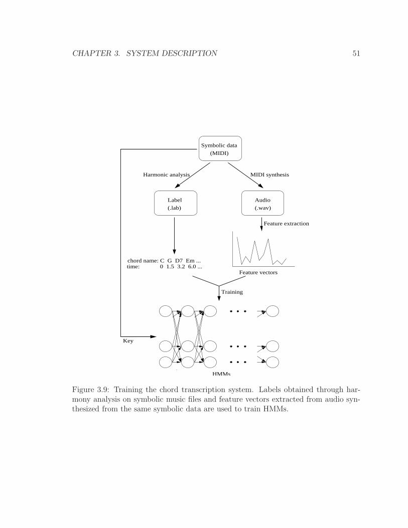
CHAPTER 3. SYSTEM DESCRIPTION 51
time: 0 1.5 3.2 6.0 ...
(MIDI)
(.lab)
Label
MIDI synthesis
Audio
(.wav)
HMMs
Training
Feature vectors
Key
chord name: C G D7 Em ...
Harmonic analysis
Symbolic data
Feature extraction
Figure 3.9: Training the chord transcription system. Labels obtained through har-mony analysis on symbolic music files and feature vectors extracted from audio syn-thesized from the same symbolic data are used to train HMMs.

CHAPTER 3. SYSTEM DESCRIPTION 52
Mozart and other composers. All classical symbolic music files are in a Humdrum
data format from the Center for Computer Assisted Research in the Humanities at
Stanford University. Humdrum is a general-purpose software system intended to help
music researchers encode, manipulate and output a wide variety of musically-pertinent
representations [39]. These files are converted to a format that can be used in the
Melisma Music Analyzer, as well as to a MIDI format using the tools developed by
Craig Sapp.1
For the second training set, we use 158 MIDI files of Beatles available from http:
//www.mididb.com.
The audio data synthesized from these symbolic music files of the classical and
Beatles data set are 26.73 hours long or 517,945 feature frames, and 5.73 hours long
or 111,108 feature frames, respectively.
We perform harmony analysis to obtain chord labels using the Melisma Music
Analyzer developed by Sleator and Temperley [94]. Melisma performs harmony anal-
ysis on a piece of music represented by an event list and extracts information about
meter, harmony and key, and so on. We configure Melisma so that it outputs a chord
name every beat and use its output as ground truth. When building key-dependent
models, we take the beginning key as a home key for an entire piece.
Temperley tests the symbolic harmony-analysis program on a corpus of excerpts
and the 48 fugue subjects from the Well-Tempered Clavier ; Melisma harmony analysis
and key extraction yields an accuracy of 83.7% and 87.4%, respectively [95].
Figure 3.10 shows the normalized distributions of chords and keys extracted from
Melisma for each training set.
We synthesize the audio files using Timidity++ (Timidity++ is a free software
synthesizer and converts MIDI files into audio files in a WAVE format.2 It uses a
sample-based synthesis technique to create harmonically rich audio as in real record-
ings.) We use the GUS (Gravis Ultra Sound) sound font, which is used by Timidity,
to synthesize the MIDI files.3 The set of instruments we use to synthesize classical
music are piano, violin, viola and cello. When rendering Beatles’ MIDI files we use
1http://extras.humdrum.net2http://timidity.sourceforge.net/3http://www.gravis.com
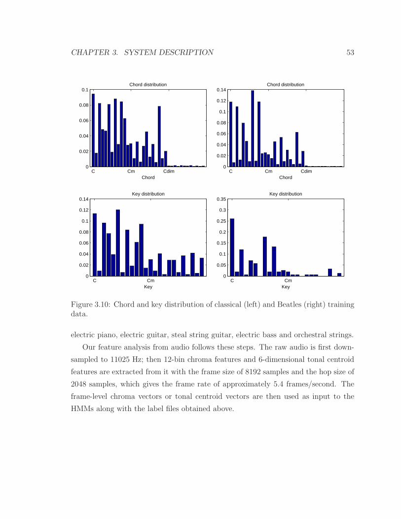
CHAPTER 3. SYSTEM DESCRIPTION 53
C Cm Cdim0
0.02
0.04
0.06
0.08
0.1Chord distribution
Chord
C Cm0
0.02
0.04
0.06
0.08
0.1
0.12
0.14Key distribution
KeyC Cm
0
0.05
0.1
0.15
0.2
0.25
0.3
0.35Key distribution
Key
C Cm Cdim0
0.02
0.04
0.06
0.08
0.1
0.12
0.14Chord distribution
Chord
Figure 3.10: Chord and key distribution of classical (left) and Beatles (right) trainingdata.
electric piano, electric guitar, steal string guitar, electric bass and orchestral strings.
Our feature analysis from audio follows these steps. The raw audio is first down-
sampled to 11025 Hz; then 12-bin chroma features and 6-dimensional tonal centroid
features are extracted from it with the frame size of 8192 samples and the hop size of
2048 samples, which gives the frame rate of approximately 5.4 frames/second. The
frame-level chroma vectors or tonal centroid vectors are then used as input to the
HMMs along with the label files obtained above.

CHAPTER 3. SYSTEM DESCRIPTION 54
3.3.2 Hidden Markov Model
We recognize chords using either 24-state (trained on Beatles music) or 36-state
HMMs (trained on classical music). Each state in our model represents a single
chord. The observation distribution is modeled by a single multivariate Gaussian—
in 12 dimensions for the chroma feature or in six dimensions for the tonal centroid
feature—defined by its mean vector µi and covariance matrix Σi, where i denotes ith
state. We assume the dimensions of the features are uncorrelated with each other, and
thus use a diagonal-covariance matrix.4 State transitions obey a first-order Markov
property; i.e., the future is independent of the past given the present state. In addi-
tion, we use an ergodic model since we allow every possible transition from chord to
chord, and yet the transition probabilities are learned.
In our model, we define 36 classes or chord types according to their sonorities
only—major, minor and diminished chords for each pitch class. We ignore the aug-
mented chords since they rarely appear in Western tonal music. We group triads and
seventh chords with the same sonority into the same category. For instance, we treat
E minor triad and E minor seventh chord as just E minor chord without differenti-
ating the triad and the seventh. Most pop or rock music, as in the Beatles, makes
use of only 24 major/minor chords, so for our experiments with popular music we
recognized only 24 chords, as done by Bello and Pickens [8].
With the labeled training data we obtain from the symbolic files, we first train our
models to estimate the model parameters. Once we learn the model parameters—
initial state probabilities, state transition probability matrix, and mean vector and
covariance matrix for each state—we recognize chords for an unknown input by ex-
tracting the feature vectors from the raw audio and applying the Viterbi [100, 30]
algorithm to the appropriate model to find the optimal path, i.e., chord sequence, in
a maximum likelihood sense.
4We tried full-covariance observation matrices, but our recognition was lower, suggestingthat we don’t have enough data.

CHAPTER 3. SYSTEM DESCRIPTION 55
Next chord
Classical Data
Cur
rent
cho
rd
C Cm Cdim
CC#D
D#EF
F#G
G#A
A#B
CmC#m
DmD#m
EmFm
F#mGm
G#mAm
A#mBm
CdimC#dim
DdimD#dim
EdimFdim
F#dimGdim
G#dimAdim
A#dimBdim
Beatles DataC
urre
nt c
hord
Next chord
C Cm Cdim
CC#D
D#EF
F#G
G#A
A#B
CmC#m
DmD#m
EmFm
F#mGm
G#mAm
A#mBm
CdimC#dim
DdimD#dim
EdimFdim
F#dimGdim
G#dimAdim
A#dimBdim 0
0.2
0.4
0.6
0.8
1.0
0
0.2
0.4
0.6
0.8
Figure 3.11: 36x36 transition probability matrices obtained from 765 pieces of classicalmusic and from 158 pieces of Beatles’ music. For viewing purpose, logarithm is takenof the original matrices. Axes are labeled in the order of major, minor and diminishedchords. The right third of these matrices are mostly zero because these musical piecesare unlikely to transition from a major or minor chord to a diminished chord, andonce in a diminished chord, the music is likely to transition to a major or minor chordagain.
3.3.3 Parameter Estimates
Figure 3.11 shows chord-to-chord transition probability matrices estimated from each
training data set. The transition matrices are strongly diagonal since a chord’s du-
ration is usually longer than the frame rate, and thus the state does not change for
several frames, which makes a transition probability to itself highest.
As further illustrated in Figure 3.12, however, the chord progressions observed in
the transition probabilities are rooted in music theory. The C major chord has the
largest probability of staying within the same state, i.e., within a C major chord,
because of faster frame rate than the rate of chord changes. But it has comparably
higher probabilities for making a transition to specific chords such as an F major,
G major, F minor or A minor chord than to others. F major and G major have
subdominant-tonic and dominant-tonic relationships with C major, respectively, and
transitions between them happen very often in Western tonal music. A C major

CHAPTER 3. SYSTEM DESCRIPTION 56
C F G Fm0
0.02
0.04
0.06
0.08
0.8
0.82
0.84
0.86Transition Probabilities
Classical DataC F G Am
0
0.02
0.04
0.06
0.88
0.9
0.92Transition Probabilities
Beatles Data
Figure 3.12: Transition probabilities from C major chord estimated from classical andfrom Beatles’ data. The X axis is labeled in the order of major, minor and diminishedchords.
chord is also a dominant chord of an F minor, and therefore a C major to F minor
transition is frequent as well. Finally, an A minor chord is a relative minor of the C
major chord, and a C-to-Am transition also occurs quite often. This tonic-dominant-
subdominant relationship is also shown in Figure 3.11 as off-diagonal lines with five
and seven semitone offsets with respect to their tonics.
Figure 3.13 shows the observation distribution parameters for chroma feature es-
timated from each training data set for a C major chord. On the left are the mean
chroma vector and diagonal covariance vector for an HMM trained on classical music,
and those for Beatles’ music are on the right. It is obvious, as expected, that they
both have three large peaks at chord tones or at C, E and G. In addition, we can also
see relatively large peaks at D and B, which come from the third harmonics of chord
tones G and E. Mean vectors and covariance matrices of tonal centroid feature are
also shown in Figure 3.14 for each data set.
Although we can estimate the model parameters for observation distribution for
each chord, the number of feature samples in training data not only varies to a
great degree from chord to chord but also is limited for some chords, as shown in

CHAPTER 3. SYSTEM DESCRIPTION 57
C C# D D# E F F# G G# A A# B0
0.05
0.1
0.15
0.2Mean Chroma Vector and Covariances for C Major Chord
Pitch ClassClassical Data
C C# D D# E F F# G G# A A# B0
0.05
0.1
0.15
0.2
Pitch ClassBeatles Data
Figure 3.13: Mean chroma vector and covariances for C major chord estimated fromclassical and from Beatles’ data. Because we use diagonal covariance, the variancesare shown with “error” bars on each dimension.
the chord distributions in Figure 3.10. This is likely to cause class statistical errors
when estimating the mean vectors and covariance matrices from the available training
samples, which may lead to overfitting. We therefore transpose all the major chords
to a single major chord no tonal center or root information, and then estimate its
probability distribution.
For example, if we wish to estimate the parameters for the C major chord, we
downshift the chroma vectors of C♯ major chord by 1, those of D major chord by
2, · · · and those of B major chord by 11, respectively. We now have more feature
samples than we had for the original C major chord. Such a transposition method
is valid because in a 12-dimensional chroma representation, only the relative spacing
between pitch classes is important, not the absolute location. Similarly, we estimate
the distribution parameters for 12 minor and 12 diminished chords. This simple
transposition method increases the number of feature samples per class to give more
accurate parameter estimates. We use this method to obtain the distribution param-
eter estimates shown in Figure 3.13 and in Figure 3.14.

CHAPTER 3. SYSTEM DESCRIPTION 58
x1 y1 x2 y2 x3 y3−0.05
0
0.05
0.1
0.15
0.2
Classical Data
Mean Tonal Centroid Vector and Covariances for C Major Chord
x1 y1 x2 y2 x3 y3−0.05
0
0.05
0.1
0.15
0.2
Beatles Data
Figure 3.14: Mean tonal centroid vector and covariances for C major chord esti-mated from classical and from Beatles’ data. Because we use diagonal covariance,the variances are shown with “error” bars on each dimension.
3.4 Experimental Results and Analysis
3.4.1 Evaluation
We test our models’ performance on two types of musical audio. First, we used Bach’s
keyboard piece (Prelude in C Major) and Haydn’s string quartet (Op.3, No.5: An-
dante, mm.1–46) as a test set of classical music. For these test data, the authors
perform harmony analysis to obtain the ground-truth annotation. For a more com-
plete test, we then test our models on the two whole albums of Beatles (CD1: Please
Please Me, CD2: Beatles For Sale) as done by Bello and Pickens [8]. Ground-truth
annotations are provided by Harte and Sandler at the Digital Music Center at the
University of London in Queen Mary.5 We reduce the class size from 36 to 24 by dis-
carding the 12 diminished chords for the Beatles’ test set since they rarely appear in
rock music. In computing frame-level scores, we only count exact matches as correct
recognition.
5http://www.elec.qmul.ac.uk/digitalmusic/
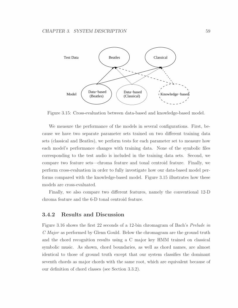
CHAPTER 3. SYSTEM DESCRIPTION 59
Knowledge−based
ClassicalBeatlesTest Data
Model (Classical)Data−based
(Beatles)Data−based
Figure 3.15: Cross-evaluation between data-based and knowledge-based model.
We measure the performance of the models in several configurations. First, be-
cause we have two separate parameter sets trained on two different training data
sets (classical and Beatles), we perform tests for each parameter set to measure how
each model’s performance changes with training data. None of the symbolic files
corresponding to the test audio is included in the training data sets. Second, we
compare two feature sets—chroma feature and tonal centroid feature. Finally, we
perform cross-evaluation in order to fully investigate how our data-based model per-
forms compared with the knowledge-based model. Figure 3.15 illustrates how these
models are cross-evaluated.
Finally, we also compare two different features, namely the conventional 12-D
chroma feature and the 6-D tonal centroid feature.
3.4.2 Results and Discussion
Figure 3.16 shows the first 22 seconds of a 12-bin chromagram of Bach’s Prelude in
C Major as performed by Glenn Gould. Below the chromagram are the ground truth
and the chord recognition results using a C major key HMM trained on classical
symbolic music. As shown, chord boundaries, as well as chord names, are almost
identical to those of ground truth except that our system classifies the dominant
seventh chords as major chords with the same root, which are equivalent because of
our definition of chord classes (see Section 3.3.2).

CHAPTER 3. SYSTEM DESCRIPTION 60
Pitc
h C
lass
12−bin Chromagram
0 2 4 6 8 10 12 14 16 18 20 22
C
C#
D
D#
E
F
F#
G
G#
A
A#
B
0 2 4 6 8 10 12 14 16 18 20 22
Tru
e
C:maj D:minsev G:domsev C:maj A:min D:domsev
D:domsev
0 2 4 6 8 10 12 14 16 18 20 22Time (seconds)
Rec
og.
C:maj D:min G:maj C:maj A:min D:maj
Figure 3.16: Frame-rate recognition results for Bach’s Prelude in C Major performedby Glenn Gould. Below 12-bin chromagram are the ground truth and the recognitionresult using a C major key HMM trained on classical symbolic music.
Table 3.1 shows the frame-level accuracy in percentage for all the test data for
various model parameters. In order to show that the data-based model performs
better than, or comparably to, the knowledge-based model, we include the frame-
rate results6 on the same Beatles’ test set by Bello and Pickens [8]. Because the
results of the knowledge-based model on the classical test data are not available,
however, we simulate them by combining the knowledge-based output distribution
parameters with the transition probabilities learned from our training data without
adaptation. We test this method on the Beatles’ test data; the difference in results
is less than 1% compared with the results of the original model [8], which uses fixed
output distribution parameters and adapts the transition probabilities for each input.
We therefore believe that the results on the classical data too are not significantly
different from what would be obtained with the original knowledge-based model.
The best result for each test material is in boldface. All the best results use a tonal
centroid vector and the model trained on the same kind of music. This is encouraging
in that the results are consistent with our expectations. If we take a closer look at
the numbers, however, we find a few items worthy of further discussions.
6Although they show higher accuracy with beat-synchronous analysis, we present hereframe-level accuracy for apple-to-apple comparison.

CHAPTER 3. SYSTEM DESCRIPTION 61
Table 3.1: Test results for various model parameters (% correct)Test Set
Model Training Set Feature Beatles ClassicalCD1 CD2 Bach Haydn
Beatles Chroma 58.56 78.21 70.92 56.20Data-based Tonal Centroid 66.89 83.87 75.03 69.07
Classical Chroma 51.82 78.77 88.31 67.69Tonal Centroid 63.81 81.73 94.56 71.98
Knowledge-based N/A Chroma 58.96 74.78 83.40 69.37
First of all, we observe a strong dependence on the training set, especially with
classical test data. This is because the model parameters, i.e., observation distri-
bution and transition characteristics are different for the two distinct musical styles.
We noticed such a genre dependency in our earlier work [57]. We also find that the
model trained on classical data is more robust to the change in musical genre of the
test input. That is, the classical model performs equally well on both test sets while
the performance of the Beatles’ model drops sharply when a different style of music is
used as an input. We believe this is because the model trained only on Beatles’ music
fails to generalize; it fails because it is only trained on music by one specific artist and
the training data set is small. On the other hand, the classical model is trained on
a larger training data set by more than eight composers, and thus performs equally
well on both test data sets.
Second, we can see that the tonal centroid feature performs better than the chroma
feature. As we mentioned earlier, a possible explanation for this is because the tonal
centroid vector is obtained by projecting the 12-bin chroma vector only on specific
interval relations, like fifths and major/minor thirds; thus, it is more suitable and
robust for identifying musical chords since these interval relations define most chords
in Western tonal music.
Our results compare favorably with other state-of-the-art systems by Harte and
Sandler [36] and by Bello and Pickens [8]. Using the same Beatles’ test data set,
Harte and Sandler obtain frame-level accuracy of 53.9% and 70.8% for CD1 and
CD2, respectively. They define 48 different triads including augmented triads, and

CHAPTER 3. SYSTEM DESCRIPTION 62
use a pattern matching algorithm for chord identification, followed by median filtering
for smoothing. Using the HMMs with 24 states for just major/minor chords, Bello
and Pickens’ knowledge-based system yields the performance of 68.55% and 81.54%
for CD1 and CD2, respectively, after they go through a pre-processing stage of beat
detection to perform a tactus-based analysis. Without a beat-synchronous analysis,
their accuracy drops down to 58.96% and 74.78% for each CD, as is shown in Table
3.1.
In computing the frame-level accuracy shown in Table 3.1, we count only exact
matches as correct. However, we believe it is more accurate to measure performance
with a tolerance of one frame. In other words, if a detected frame boundary or
its neighbor is equal to the ground truth, we classify it as a correct match. This
assumption is fair since the segment boundaries are generated by humans listening
to audio, and thus they are not razor sharp. Using this error metric, the accuracy
of our key-dependent tonal centroid models rises to 69.15% and 86.66% for Beatles’
CD1 and CD2, respectively.
3.5 Summary
In this chapter, we have described a HMM-based chord recognition system, and we
have demonstrated that symbolic music data, such as MIDI files, can be used to
train machine-learning models like HMMs, with a performance that matches the best
knowledge-based approach. The key idea behind our data-based approach was to use
automatic generation of labeled training data to free researchers from the laborious
task of manual annotation.
In order to accomplish this goal, we used symbolic data to generate label files,
as well as to synthesize audio files. The rationale behind this idea was that it is
far easier and more robust to perform harmony analysis on the symbolic data than
on the raw audio data since symbolic music files, such as MIDI, contain noise-free
pitch information. In addition, by using a sample-based synthesizer, we created audio
files that have harmonically rich spectra as in real acoustic recordings. This nearly
labor-free procedure to obtain labeled training data enabled us to build a generalized

CHAPTER 3. SYSTEM DESCRIPTION 63
model, resulting in improved performance.
As feature vectors, we first used conventional 12-bin chroma vectors, which have
been successfully used by others in chord recognition. In addition, we tried another
feature vector called tonal centroid which yielded better performance.
Each state in our HMM was modeled by a multi-variate, single Gaussian com-
pletely represented by its mean vector and a diagonal covariance matrix. We defined
36 classes or chord types in our models, which include for each pitch class three dis-
tinct sonorities—major, minor and diminished. We treated seventh chords as their
corresponding root triads and disregarded augmented chords since they very rarely
appear in Western tonal music.
In order to examine the generality of our approach, we obtained two different
model parameters trained on two musically distinct data sets. Experiments with
various kinds of unseen test input, all real acoustic recordings, showed that there is
positive correlation between the test and the training data. In other words, the results
were better when the test and training data are of the same kind. This dependency
on the training set, however, was less significant when the size of the training set
was larger. This in turn suggests that we can generalize our model with even larger
amount of training data.
Bello and Pickens showed approximately an 8% performance increase using beat-
synchronous analysis. While there is some chance for increased errors if beat-tracking
is done incorrectly, we believe that this result is orthogonal to the arguments pre-
sented in this paper. Thus a state-of-the-art system for chord recognition should
combine the data-driven approach described here with tonal centroid features and
beat-synchronous analysis.
The one and only goal of the system described so far was chord recognition.
However, musical chord is closely related to a key in tonal music. Therefore, if we
know the key of a musical piece, we expect that certain chords will more likely appear
than the others, or we can infer a musical key by observing the progression of chords
over time. Furthermore, musical genre is also dependent on the use of chords and
their progression. For instance, rock music makes extensive use of I, IV and V chords,
and the most typical chord progression found in blues music is I-VI-I-V-I.

CHAPTER 3. SYSTEM DESCRIPTION 64
In the next chapter, we present how we can extend the chord recognition system
described above to identify or provide information as to other musical attributes such
as key or genre and to improve chord recognition

Chapter 4
Extension
4.1 Introduction
In this chapter, we present two extensions of the HMM-based chord recognition system
described in Chapter 3 that increase chord recognition performance and provide other
useful information such as key or genre. The rationale behind these extensions —
key-dependent and genre-specific HMMs — is that musical chords are closely related
to key or genre, and therefore a priori information as to key or genre makes chord
recognition easier, especially when the feature vectors appear similar as in the related
chords such as a major-minor pair sharing the root note (C major and C minor) or
relative major-minor chords (C major and A minor). However, we don’t need to have
such prior information beforehand. In fact, by building key- or genre-specific models
and computing the likelihood of each model, we can estimate the key or identify the
genre of the input audio. Furthermore, we show that the selected key or genre model
outperforms the generic model described in the previous chapter.
65

CHAPTER 4. EXTENSION 66
4.2 Key-dependent HMMs
4.2.1 System
In Western tonal music, a song’s key and chords are closely related; thus, knowing the
key of a piece provides valuable information about the chords as well. For instance, if
a musical piece is in the key of C major, then we can expect frequent appearances of
chords such as C major, F major and G major, which correspond to the tonic, sub-
dominant and dominant chord, respectively. On the other hand, F♯minor or A♭ major
chord will seldom appear, since neither has any harmonic function in a C major key.
Based on this close relationship between musical key and chords inherent in Western
tonal music, this thesis proposes key-dependent HMMs trained on synthesized audio
for chord recognition and key estimation [60, 61].
An important advantage of using symbolic music files is that other information,
such as the key or the tempo, comes for free. We therefore build key-dependent
models using the key information already contained in the symbolic data. We define
major/minor keys for each pitch class, resulting in 24 different HMMs. After building
24 key models, λk, 1 ≤ k ≤ 24, we simultaneously perform key estimation and chord
recognition of an unknown input as follows. First, given an acoustic input, we extract
the observation sequence O = {O1O2 · · ·OT} of appropriate feature. Then, we calcu-
late the model likelihoods for all 24 key-dependent models, P (O,Q|λk), 1 ≤ k ≤ 241. We then estimate the key by selecting the key model whose likelihood is highest,
i.e.,
k∗ = argmax1≤k≤24
P (O,Q|λk). (4.1)
By using the Viterbi algorithm in Equation 4.1, however, we not only estimate
the key k∗, but we also obtain the optimal state path Q∗ = {Q1Q2 · · ·QT}, which is
an estimate of the frame-level chord sequence. This process is illustrated in Figure
1An algorithm for efficient computation of P (O,Q|λk), also known as Viterbi decoding,is described in Appendix A.

CHAPTER 4. EXTENSION 67
= optimal state path= chord sequence
Observation:Acousticinput
Featureanalysis
HMM 1
HMM 2
HMM K(λK)
O = O1O2 · · ·OT Q∗ = Q1Q2 · · ·QT
k∗ = argmaxk Pr(O, Q|λk)
Pr(O, Q|λK)
Pr(O, Q|λ2)
...
Pr(O, Q|λ1)
(λ1)
(λ2)
Figure 4.1: System for key estimation and chord recognition using key-dependentmodels (K = 24).
4.1.
Although similar systems for key estimation were previously proposed by others
using the HMMs with chroma features as observation [81, 80], the one and only goal of
these systems was key estimation; the states in the HMMs had no musical meanings.
However, in our system, we treat the hidden states as chords, and therefore we also
identify the chord sequence by finding the optimal state path using a Viterbi decoder
when computing the likelihood of the key model.
4.2.2 Parameter Estimates
We use the same sets of training data we used in Chapter 3 (classical and the Beatles).
Figure 4.2 shows the distribution of 24 keys of the whole training data set. Because
we assume there is no key modulation within a piece, each musical piece is assigned
a single key. Therefore, it is not impossible that there are keys without any instances
or very few, if any, which might result in poor models. For example, there is only one
instance of A♭ minor key, while there are 174 pieces of music in the key of C major.
Such a discrepancy in the class size will result in statistical errors when estimating
the model parameters.
Therefore, in the same manner we estimate observation distribution parameters
for each chord, by transposing all the major[minor] chords to C major[minor] chord
and transposing back to all the other major (minor) chords, we also perform circular
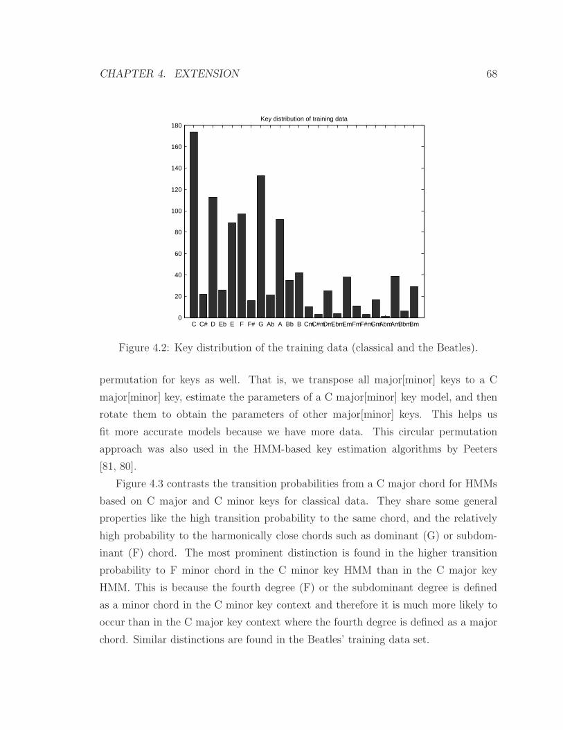
CHAPTER 4. EXTENSION 68
C C# D Eb E F F# G Ab A Bb B CmC#mDmEbmEmFmF#mGmAbmAmBbmBm0
20
40
60
80
100
120
140
160
180Key distribution of training data
Figure 4.2: Key distribution of the training data (classical and the Beatles).
permutation for keys as well. That is, we transpose all major[minor] keys to a C
major[minor] key, estimate the parameters of a C major[minor] key model, and then
rotate them to obtain the parameters of other major[minor] keys. This helps us
fit more accurate models because we have more data. This circular permutation
approach was also used in the HMM-based key estimation algorithms by Peeters
[81, 80].
Figure 4.3 contrasts the transition probabilities from a C major chord for HMMs
based on C major and C minor keys for classical data. They share some general
properties like the high transition probability to the same chord, and the relatively
high probability to the harmonically close chords such as dominant (G) or subdom-
inant (F) chord. The most prominent distinction is found in the higher transition
probability to F minor chord in the C minor key HMM than in the C major key
HMM. This is because the fourth degree (F) or the subdominant degree is defined
as a minor chord in the C minor key context and therefore it is much more likely to
occur than in the C major key context where the fourth degree is defined as a major
chord. Similar distinctions are found in the Beatles’ training data set.

CHAPTER 4. EXTENSION 69
C F G Fm0
0.02
0.04
0.06
0.08
0.85
0.87
0.89
C Major HMMC F G Fm
0
0.02
0.04
0.06
0.08
0.8
0.82
0.84Transition Probabilities from C Major Chord
C Minor HMM
Figure 4.3: Transition probabilities from a C major chord in C major key and in Cminor key HMM from classical data. The X axis is labeled in the order of major,minor and diminished chords. Compare this to the generic model shown in Figure3.12.
Such key-specific transition probability matrices help us make a correct decision,
particularly in situations where the observation feature vectors are ambiguous. For
example, those chords in relations such as relative major/minor pairs share two notes
in common, and thus their observation vectors look quite similar, which may cause
great confusion. Discriminating the transition probabilities even from the same chord
by using key-specific HMMs helps avoid mis-recognition caused by the confusion
described above.
Even with key-dependent HMMs, however, we use mean feature vectors and co-
variance matrices that are obtained from the universal, key-independent HMM be-
cause we believe the chord quality remains the same, independent of key context. For
instance, the sonic quality of a C major chord in C major key will be the same as
that of a C major chord in A minor key. What differs in each key is the distribution
of chords, as well as their transition probabilities.
Although changes in key within a piece of music, or modulations, are not rare

CHAPTER 4. EXTENSION 70
in Western tonal music, we did not take them into account in building the models
because modulations occur mostly between harmonically closely-related keys such as
parallel, relative major/minor keys or those in fifth relation, and therefore don’t cause
significant alterations in chord distribution or progression characteristics.
4.2.3 Results and Discussion
We used the same evaluation setup as we did in Chapter 3, and made comparison with
the knowledge-based model. Table 4.1 shows the frame-level accuracy in percentage
for the Beatles test data for various model parameters. Results in parenthesis are
obtained using a key-dependent model; the best result for each test material is in
boldface. Comparison between a genric and a key-dependent model is also illustrated
in Figure 4.4.
Table 4.1: Test results for various model parameters (% correct). In parenthesis areaccuracies of key-dependent models.
Test SetModel Training Set Feature Beatles
CD1 CD2Beatles Chroma 58.56 (57.89) 78.21 (78.38)
Data-based Tonal Centroid 66.89 (67.50) 83.87 (85.24)Classical Chroma 51.82 (52.46) 78.77 (79.35)
Tonal Centroid 63.81 (64.79) 81.73 (83.19)Knowledge-based N/A Chroma 58.96 74.78
We observe the overall effect that a key-dependent model has on the performance.
Except for one case (chroma feature; Beatles CD1), we find that a key-dependent
model always increases performance. As mentioned in Section 4.2.1, chord progression
is based on the musical key; therefore, knowing the key helps determine which chord
is more likely to follow. Such an example is illustrated in Figure 4.5.
This Figure shows an excerpt of frame-level recognition results of the Beatles’ song
Eight Days A Week, which is in the key of D major. The results of the D major key
model are shown with circles, and those of a key-independent model are indicated
with x’s. We observe that a key-independent model makes a wrong transition from

CHAPTER 4. EXTENSION 71
1 2 3 450
55
60
65
70Results on CD1
Acc
urac
y (%
)
Model1 2 3 4
76
78
80
82
84
86Results on CD2
Acc
urac
y (%
)
Model
generickey−dependent
generickey−dependent
Figure 4.4: Comparison of a generic model with a key-dependent model. Modelnumbers on the x-axis denote: 1) chroma, trained on Beatles; 2) tonal centroid,trained on Beatles; 3) chroma, trained on classical; 4) tonal centroid, trained onclassical.
G major to D minor chord near 158 seconds while the D major key model correctly
switches to D major chord. As mentioned, D major and D minor chord have a parallel
major/minor relation. They share two chord tones—tonic and dominant or D and
A—which make the observation vector of those chords look similar, and thus causes
similar output probabilities. In the D major key, however, scale degree 1 or D is
a tonic center and is defined as a major chord, although it is possible to use a D
minor chord. Therefore, a D major chord occurs more often in D major key than
for example, in the C major or in the D minor key, resulting in higher transition
probability to it than to other chords. For the same reason, since a D minor chord
is rarely used in the D major key, it is less probable. This is clearly indicated in
Table 4.2, which shows transition probabilities learned from the data. As shown, a
transition from G major to D major chord is almost three times more likely in the
key-specific model than in the key-independent model, while a G major to D minor
chord transition is three times less likely.
We performed a quantitative evaluation on the key estimation algorithm. We
compared our results to manually-labeled ground truth for the Beatles’ test set [84].

CHAPTER 4. EXTENSION 72
152 153 154 155 156 157 158 159 160 161 162 163C
C#
D
D#
E
F
F#
G
G#
A
A#
B
Cm
C#m
Dm
D#m
D:maj
Frame−rate recognition results
Time (seconds)
Cho
rd
D:maj G:maj
D major key model
Universal model
Figure 4.5: Frame-rate recognition results from Beatles’ Eight Days A Week. In circlesare the results of D major key model and in x’s are those of universal, key-independentmodel. Ground-truth labels and boundaries are also shown.
Of all the 30 pieces (28 Beatles and 2 classical) in the test set, our system correctly
estimated 29 of them, achieving an accuracy of 97%. The only song our system mis-
recognized was A Taste of Honey, which is in the key of F♯ minor. Our algorithm
recognized it as a E major key instead, which is not a related key. One possible
explanation is that the extensive use of E, A and B major chords strongly implies the
key of E major because those chords form the most important functions in tonal har-
mony, namely tonic, subdominant and dominant of E major key. The 97% accuracy
for finding key from audio is very encouraging, although the test set was small.
We also tested our key estimation system on Bach’s Well Tempered Clavier I,
which consists of 24 preludes and fugues in each key. Using our algorithm, 41 out
of total 48 pieces were correctly identified, corresponding to 85.42% of accuracy. Six
of seven mis-recognized keys were related keys (five relative major-minor and one

CHAPTER 4. EXTENSION 73
Table 4.2: Transition probabilities from G major to D major and D minor chord ineach model
Model Transition ProbabilityG:maj→D:maj G:maj→D:min
D major key (A) 0.0892 0.0018Key-independent (B) 0.0332 0.0053
Ratio (A/B) 2.67 0.34
parallel major-minor). MIREX 2 scoring system assigns 1 point for correct keys, 0.5
for perfect fifth, 0.3 for relative keys and 0.2 for parallel keys. Using these scores,
our system achieves 88.96% for key estimation. Although the test set is small to
provide more complete results, these accuracies are similar to other state-of-the-art
key-finding systems.3
4.3 Genre-Specific HMMs
4.3.1 System
When our previous systems [60] were tested with various kinds of input, the chord
recognition performance was greatest when the input audio was of the same kind
as the training data set, suggesting the need to build genre-specific models. This
is because not only different instrumentations cause the feature vector to vary, but
also the chord progression, and thus the transition probabilities, are very different
from genre to genre. For example, blues music makes extensive use of I (tonic),
V (dominant) and IV (subdominant) chords, and therefore the transitions between
these chords are very frequent. Thus the state-transition probability matrix trained
on blues music will be different from those trained on other types of music.
The overall system shown in Figure 4.6 is almost identical to key-dependent HMMs
shown in Figure 4.1, except that key models are replaced with genre models. In
addition, while there are 24 fixed number of key models, the number of genres may
2Music Information Retrieval Evaluation eXchange. http://www.music-ir.org3The best system in MIREX 2005 Audio Key Finding achieved 89.55% accuracy using
1,252 MIDI-synthesized audio files as a test set.

CHAPTER 4. EXTENSION 74
= optimal state path= chord sequence
Observation:Acousticinput
Featureanalysis
HMM 1
HMM 2
HMM G
O = O1O2 · · ·OT Q∗ = Q1Q2 · · ·QT
Pr(O, Q|λG)
Pr(O, Q|λ2)
...
Pr(O, Q|λ1)
(λ1)
(λ2)
(λG)
g∗ = argmaxg Pr(O, Q|λg)
Figure 4.6: Chord recognition system using genre-specific HMMs (G = 6).
Table 4.3: Online sources for MIDI filesGenre Online source
Keyboard http://www.classicalarchives.com
Chamber http://www.classicalarchives.com
Orchestral http://www.classicalarchives.com
Rock http://www.mididb.com
Jazz http://www.thejazzpage.de
Blues http://www.davebluesybrown.com
vary according to the training data.
4.3.2 Parameter Estimates
As has been described in Section 4.3.1, we build an HMM for each genre. While
the genre information is not explicitly contained in the symbolic music files, as is
the key information, most MIDI files are categorized by their genres, and we can use
them to obtain different training data sets by genres. We define six musical genres
including keyboard, chamber, orchestral, rock, jazz, and blues. Table 4.3 shows the
online sources where we acquired the MIDI files.
The total number of MIDI files and synthesized audio files used for training is
4,212, which correspond to 348.73 hours of audio or 6,758,416 feature vector frames.
Table 4.4 shows in more detail the data sets used to train each genre model.
Figure 4.7 shows the 36×36 transition probability matrices for rock, jazz, and

CHAPTER 4. EXTENSION 75
Table 4.4: Training data sets for each genre modelGenre # of MIDI/Audio files # of frames Audio length (hours)
Keyboard 393 1,517,064 78.28Chamber 702 1,224,209 63.17Orchestral 319 1,528,796 78.89
Rock 1,046 1,070,752 55.25Jazz 1,037 846,006 43.65Blues 715 571,589 29.49All 4,212 6,758,416 348.73
blues model after training. Although they are all strongly diagonal because the rate
at which chord changes is usually longer than the frame rate, we still can observe
the differences among them. For example, the blues model shows higher transition
probabilities between the tonic (I) and the dominant (V) or subdominant (IV) chord
than the other two models, which are the three chords almost exclusively used in
blues music. This is indicated by darker off-diagonal lines 5 or 7 semitones apart
from the main diagonal line. In addition, compared with the rock or blues model, we
find that the jazz model reveals more frequent transitions to the diminished chords,
as indicated by darker last third region, which are rarely found in rock or blues music
in general.
We also see the difference in the observation distribution for each genre, as shown
in Figure 4.8. Figure 4.8 displays the mean tonal centroid vectors and covariances of
C major chord in the keyboard, chamber, and in the orchestral model, respectively,
where the observation distribution of the chord was modeled by a single Gaussian.
We believe that using model parameters specific to each genre will increase the
chord recognition accuracy when the correct genre model is selected. The success of
this hypothesis will be described in Section 4.3.3.

CHAPTER 4. EXTENSION 76
Rock model
Cho
rd N
ame
12 24 36
CC#DD#EFF#GG#AA#BCmC#mDmD#mEmFmF#mGmG#mAmA#mBmCdimC#dimDdimD#dimEdimFdimF#dimGdimG#dimAdimA#dimBdim
Jazz model
12 24 36
12
24
36
Blues model
12 24 36
12
24
36
Figure 4.7: 36×36 transition probability matrices of rock (left), jazz (center), andblues (right) model. For viewing purpose, logarithm was taken of the original matri-ces. Axes are labeled in the order of major, minor, and diminished chords.
4.3.3 Experimental Results and Analysis
Evaluation
We tested our models’ performance on the two whole albums of Beatles (CD1: Please
Please Me, CD2: Beatles For Sale) as done by Bello and Pickens [8], each of which
contains 14 tracks. Ground-truth annotations were provided by Harte and Sandler
at the Digital Music Center at University of London in Queen Mary.4
In computing scores, we only counted exact matches as correct recognition. We
tolerated the errors at the chord boundaries by having a time margin of one frame,
which corresponds approximately to 0.19 second. This assumption is fair since the
segment boundaries were generated by human by listening to audio, which cannot be
razor sharp.
To examine the dependency of the test input on genres, we first compared the
each genre model’s performance on the same input material. In addition to 6 genre
models described in Table 4.4, we built a universal model without genre dependency
where all the data were used for training. This universal, genre-independent model
4http://www.elec.qmul.ac.uk/digitalmusic/
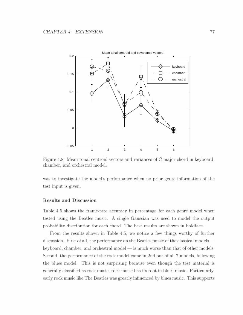
CHAPTER 4. EXTENSION 77
1 2 3 4 5 6−0.05
0
0.05
0.1
0.15
0.2Mean tonal centroid and covariance vectors
keyboard
chamber
orchestral
Figure 4.8: Mean tonal centroid vectors and variances of C major chord in keyboard,chamber, and orchestral model.
was to investigate the model’s performance when no prior genre information of the
test input is given.
Results and Discussion
Table 4.5 shows the frame-rate accuracy in percentage for each genre model when
tested using the Beatles music. A single Gaussian was used to model the output
probability distribution for each chord. The best results are shown in boldface.
From the results shown in Table 4.5, we notice a few things worthy of further
discussion. First of all, the performance on the Beatles music of the classical models —
keyboard, chamber, and orchestral model — is much worse than that of other models.
Second, the performance of the rock model came in 2nd out of all 7 models, following
the blues model. This is not surprising because even though the test material is
generally classified as rock music, rock music has its root in blues music. Particularly,
early rock music like The Beatles was greatly influenced by blues music. This supports

CHAPTER 4. EXTENSION 78
Table 4.5: Test results for each model with major/minor/diminished chords (36 states,% accuracy)
Model Beatles CD1 Beatles CD2 TotalKeyboard 38.674 73.106 55.890Chamber 30.557 73.382 51.970Orchestral 18.193 57.109 37.651
Rock 45.937 77.294 61.616Jazz 43.523 76.220 59.872Blues 48.483 79.598 64.041All 24.837 68.804 46.821
Table 4.6: Test results for each model with major/minor chords only (24 states, %accuracy)
Model Beatles CD1 Beatles CD2 TotalKeyboard 43.945 73.414 58.680Chamber 43.094 79.593 61.344Orchestral 37.238 77.133 57.186
Rock 60.041 84.289 72.165Jazz 44.324 76.107 60.216Blues 52.244 80.042 66.143All 51.443 80.013 65.728
our hypothesis that the corresponding or similar genre model will increase the chord
recognition accuracy.
Knowing that the test material does not contain any diminished chords, we did
another experiment with the class size reduced down to just 24 major/minor chords
instead of full 36 chord types. The results are shown in Table 4.6.
With fewer chord types, we can observe that the recognition accuracy increased
by as much as 20% for some model. Furthermore, the rock model outperformed
all other models, again verifying our hypothesis on genre-dependency. This in turn
suggests that if the type of the input audio is given, we can adjust the class size of
the corresponding model to increase the accuracy. For example, we may use 36-state
HMMs for classical or jazz music where diminished chords are frequently used, but
use only 24 major/minor chord classes in case of rock or blues music, which rarely
uses diminished chords.
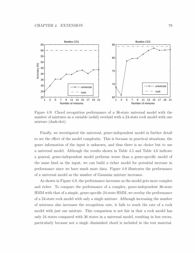
CHAPTER 4. EXTENSION 79
1 3 5 7 9 11 13 15 17 19 2120
25
30
35
40
45
50
55
60
65
Number of mixtures
Acc
urac
y (%
)
Beatles CD1
1 3 5 7 9 11 13 15 17 19 2165
70
75
80
85
Number of mixtures
Beatles CD2
universal
rock
universal
rock
Figure 4.9: Chord recognition performance of a 36-state universal model with thenumber of mixtures as a variable (solid) overlaid with a 24-state rock model with onemixture (dash-dot).
Finally, we investigated the universal, genre-independent model in further detail
to see the effect of the model complexity. This is because in practical situations, the
genre information of the input is unknown, and thus there is no choice but to use
a universal model. Although the results shown in Table 4.5 and Table 4.6 indicate
a general, genre-independent model performs worse than a genre-specific model of
the same kind as the input, we can build a richer model for potential increase in
performance since we have much more data. Figure 4.9 illustrates the performance
of a universal model as the number of Gaussian mixture increases.
As shown in Figure 4.9, the performance increases as the model gets more complex
and richer. To compare the performance of a complex, genre-independent 36-state
HMM with that of a simple, genre-specific 24-state HMM, we overlay the performance
of a 24-state rock model with only a single mixture. Although increasing the number
of mixtures also increases the recognition rate, it fails to reach the rate of a rock
model with just one mixture. This comparison is not fair in that a rock model has
only 24 states compared with 36 states in a universal model, resulting in less errors,
particularly because not a single diminished chord is included in the test material.

CHAPTER 4. EXTENSION 80
As stated above, however, given no prior information regarding the kind of input
audio, we can’t take the risk of using a 24-state HMM with only major/minor chords
because the input may be classical or jazz music in which diminished chords appear
quite often.
The above statements therefore suggest that genre identification on the input
audio must be done in advance in order to be able to use genre-specific HMMs for
better performance. It turns out, however, that we don’t need any other sophisticated
genre classification algorithms or different feature vectors like MFCC, which is almost
exclusively used for genre classification. Given the observation sequence from the
input, when there are several competing models, we can select the correct model
by choosing one with the maximum likelihood using a forward algorithm or Viterbi
decoder. It is exactly the same algorithm as one used in isolated word recognition
systems described by Rabiner [86]. Once the model is selected, we can apply the
Viterbi decoder to find the most probable state path, which is identical to the most
probable chord sequence. Using this method, our system successfully identified 24
tracks as rock music out of total 28 tracks, which is 85.71% accuracy. What is
noticeable and interesting is that the other four mis-classified songs are all classified
as blues music in which rock music is known to have its root. In fact, they all are
very blues-like music, and some are even categorized as “bluesy”. This suggests that
perhaps rock and blues should be merged into one genre — blues and rock.
4.4 Summary
In this chapter, we have demonstrated that we can extend the basic chord recognition
system using an HMM described in Chapter 3 to build key- or genre-specific HMMs
and train them with synthesized audio. Easily generating a large amount of labeled
training data from symbolic music files allows us to build such richer models.
Based on the close relationship between key and chord in Western tonal music,
we built 24 key-dependent HMMs, one for each key, using key information derived
from the symbolic music files. Given an acoustic input, our system performs feature
analysis and a sequence of observation is input to the key-dependent HMMs. Using
CHAPTER 4. EXTENSION 81
a Viterbi decoder, we estimate the key by selecting the model with the maximum
likelihood; at the same time, we recognize frame-level chord sequence because it is
the same as the optimal state path in a selected key model. Experimental results
on real acoustic recordings show that a key-dependent model not only gives the key
information of an input, but also increases the chord recognition accuracy, yielding
very promising results on both musical tasks.
Although genre information is not explicitly encoded in symbolic music files as key
is, it is not difficult to find symbolic music files categorized by genres. We therefore
build genre-specific HMMs, similar to key-dependent HMMs, resulting in improved
performance with much simpler models than a more complex, genre-independent
model.
Using synthesized audio to train the models successfully capture genre-specific
musical characteristics seen in real acoustic recordings, and experimental results show
that the performance is best when the model and the input are of the same kind, which
supports our hypothesis on the need for building genre-specific models. Another
great advantage of the present approach is that we can also predict the genre — even
though the identification rate is not that of other state-of-the-art systems whose only
purpose is genre identification — of the input audio by computing the likelihoods
of different genre models as is done in isolated word recognizers. This way, we not
only extract chord sequence but also identify musical genre at the same time, without
using any other algorithms or feature vectors. This is important because we integrate
two distinct musical tasks—i.e. chord recognition and genre classification—into one
framework.
In the next chapter, we introduce an enhanced model for chord recognition —
discriminative HMM.

Chapter 5
Advanced Model
5.1 Introduction
In this chapter, we present an advanced approach that combines a powerful discrim-
inative algorithm for chord classification with the HMM smoothing for finding the
optimal state path. This model is not finalized yet and we haven’t had enough ex-
periments to provide complete quantitative evaluations. However, we believe this
model is based on more advanced statistical learning algorithms and therefore will
outperform the basic models.
5.2 Discriminative HMM
In our HMM described in Chapter 3, we modeled each state (i.e., chord) using a
multivariate Gaussian, which is a generative approach; that is, we try to build each
chord model first, based on the labeled training data. Then we compute the poste-
rior probabilities that the observation is generated by each model, given the input
observation, using Bayes’ rule [90]. Mathematically, we compute for each chord model
p(y|x) =p(x|y)p(y)
p(x), (5.1)
82

CHAPTER 5. ADVANCED MODEL 83
where x is an input observation and y is a class or chord. In a generative model, we
learn p(x|y) and p(y) from the data. p(y) is called class priors and is given by
p(y) =∑
y
p(x|y). (5.2)
In fact, we don’t even need to know the marginal likelihood p(x) to compute the
posterior p(y|x) since from Equation 5.1, we have
argmaxy
p(y|x) = argmaxy
p(x|y)p(y)
p(x)
= argmaxy
p(x|y)p(y). (5.3)
A generative model such as a Gaussian model is based on assumptions about
how the data is generated. For example, if the distribution of the data is indeed
Gaussian, the Gaussian model is asymptotically efficient, especially for a large amount
of training data [72].
On the other hand, in a discriminative model no such assumptions are made
and therefore it is more robust and less sensitive to incorrect modeling assumptions.
Instead of computing the posterior distributions p(y|x) from the model likelihood
p(x|y) and the prior p(y) as in a generative model, the discriminative model tries to
learn the boundary that discriminates p(y|x) directly from the training data.
Support vector machines (SVMs) are among the most popular discriminative mod-
els and have recently been used with a great success in a number of applications,
including music applications such as genre classification [5], chord recognition [69],
mood classification [53] and instrument identification [44] and so on.
A hybrid model has been used in speech recognition to combine the discrimina-
tive power of SVMs with the ability of HMMs to efficiently represent the temporal
dynamics of speech [47, 48]. However, the output of an SVM is a distance measure
between the observation and the optimal decision boundary, which is not suitable
for an HMM which requires posterior probabilities. Platt proposed an algorithm to

CHAPTER 5. ADVANCED MODEL 84
estimate these emission probabilities from the SVM output f(x) using Gaussians of
equal variance and then computing the probability of the class given the output by
using Bayes’ rule, yielding [83]
p(y = 1|x) = g(f(x), A,B)
≡1
1 + exp(Af(x) +B). (5.4)
Platt also proposed an algorithm to estimate the parameters A,B in Equation 5.4
using maximum likelihood estimation. Interested readers are encouraged to see [83].
Finally, since SVMs are binary classifiers, we need to find a method to classify
more than two classes as in our chord recognition (we have 36 classes). There are two
widely used approaches for multi-class SVMs: one-vs-rest approach and one-vs-one
approach [38, 91]. Although the one-vs-one approach requires N(N −1)/2 number of
SVMs for N -class classification (e.g., 630 SVMs for our application), it takes much
less time to train them all since the time to train one SVM depends super-linearly on
the number of training samples.
Using the hybrid model described above, Kruger et al. achieved better results on
phoneme recognition, even with less training samples than the HMM with Gaussian
mixture models, which was trained on the full training set [47, 48].
We believe that this hybrid SVM/HMM approach, which has the best of both
worlds, will help increase our chord recognition performance because recognizing the
sequence of chords also does benefit from temporal modeling represented by an HMM
through state-transition probabilities, and yet the powerful discriminative algorithms
like SVMs are likely to help compute the posterior probabilities more accurately.
5.2.1 Experiments and Discussions
We performed an initial experiment on the discriminative HMMs for chord recogni-
tion. We used the same classical data for training and the Beatles’ two albums for
testing, which were also used in Chapter 3. The average % accuracy was 57.68% for

CHAPTER 5. ADVANCED MODEL 85
the CD1 (Please Please Me) and 76.72% for the CD2 (Beatles For Sale). These num-
bers are low compared to those by the basic models, which are 63.81% and 81.73%
for each album, respectively.
However, we used only 1000 training samples for each class (chord) due to the
extensive amount of time it takes to train 630 SVMs (we used one-versus-one approach
for multi-class classification as explained in Section 5.2). This diluted training data set
is just 7% of the full training set used in the original HMMs with Gaussian modeling.
We hope that the performance of the discriminative HMMs increases as we increase
the size of the training data.
One interesting observation worthy of further discussion is that the classification
without HMM smoothing is better with the SVMs than with the Gaussian models;
that is, the SVMs outperform the Gaussian models in classifying the given obser-
vations to correct classes (chords), using only the posterior probabilities. However,
when we integrate the posterior distribution into an HMM framework with the state-
transition probabilities and compute the optimal state path using a Viterbi decoder,
the HMM with the Gaussian models yields the better results. We haven’t fully investi-
gated this yet, but a possible explanation is that the posterior probabilities estimated
from the distance measures from the SVMs aren’t accurate. We plan to try different
estimation algorithms in the future.
For more complete and fair comparison, we built the Gaussian models using only
7% of the full training set as we did with the SVMs, and performed the experiments
on the same test set. Table 5.1 shows the results.
Table 5.1: Comparison of SVMs and Gaussian models trained on the same amountof training data (% accuracy)
Model Test dataCD1 CD2 Average
SVMs (diluted, 1/15) 57.68 76.72 67.20Gaussian models (diluted, 1/15) 46.24 78.63 62.44
Gaussian models (full set) 63.81 81.73 72.77
As is shown in Table 5.1, SVMs outperform the Gaussian models by 5% under
the same condition; i.e., when the amount of training data to train both models is

CHAPTER 5. ADVANCED MODEL 86
the same. The sharp drop in accuracy (from 72.77% to 62.44%) with the Gaussian
models trained on fewer data indicates the weakness of Gaussian model when the data
is insufficient because in generative models, the less data we have, the more difficult
it becomes to correctly estimate the model parameters.
5.3 Summary
In this chapter, we presented a hybrid model for chord recognition based on the
original HMM. The hybrid model uses powerful discriminative algorithms to compute
the posterior probabilities that the given observation vector belongs to each chord.
To this end, we use SVMs which have proved to be very successful in many other
classification problems, including several music applications. In order to estimate the
emission probability distribution required in the HMM smoothing stage, we use a one-
versus-one approach, which requires 36 × (36 − 1)/2 = 630 support vector machines
to be trained. The experiments show promising results: when we train the SVMs and
the Gaussian models with the same amount of diluted training data (approximately
1/15 of the full data), the SVMs outperform the Gaussian models by 5%.
In the following chapter, we demonstrate several practical applications where the
key and the chord sequence recognized by the system are directly or indirectly used.

Chapter 6
Applications
6.1 Introduction
There are a number of practical applications where content-based music information
retrieval becomes very useful. These applications include audio coversong finding,
structural analysis, music segmentation/clustering, audio thumbnailing, query-by-
humming (QBH), query-by-example (QBE), music recommendation, playlist genera-
tion, to name a few.
In this chapter, we demonstrate that we can use a sequence of chords, which is
extracted using the models described in Chapter 3 and Chapter 4, in some of the
applications stated above.
6.2 Audio Cover Song Identification
A cover song is defined as a song performed by an artist different from the origi-
nal artist.1 Identifying cover songs given an original as a seed/query or finding the
original given a cover version from the raw audio is a challenging task, and it has
recently drawn attention in the Music Information Retrieval community. A cover
song is different from its original in terms of many musical attributes such as tempo,
dynamics, melody, key, timbre, and/or instrumentation, and thus the raw waveform
1http://www.secondhandsongs.com/wiki/Guidelines/Cover
87
CHAPTER 6. APPLICATIONS 88
or its frequency-domain representation like spectrogram is very different from each
other. Therefore, identifying cover songs requires a robust feature set that remains
largely unchanged under various acoustical changes caused by various musical prop-
erties mentioned above.
Harmonic progression or chord sequence is a robust mid-level representation that
is largely preserved under such musical variations. While other musical details such
as melody, tempo, and/or timbre may vary from one to another, their harmonic
progression over time undergoes minor changes compared with the others because it
was built by conforming to fundamental rules found in Western tonal music. Using
harmonic progression or chord sequence as a feature set has more advantages: first,
once the chord sequence is extracted from the raw audio, it is just a uni-dimensional
string, and thus is computationally very efficient to process. Second, in computing
the distance between two chord sequences, we can also define the transition cost from
a chord to another as well as the cost of being in aligned states since, for example,
a transition from a G major chord to a C major chord is much more probable than
a transition from a G major to a A♯ minor in Western tonal harmony. Defining
such transition cost would not be possible or meaningful unless we use explicit chord
names. Experiments show that adding a transition cost to an alignment cost improves
performance of the proposed system.
In the next section, we review other related works on cover song finding.
6.2.1 Related Work
Pickens and Crawford proposed a system for polyphonic music retrieval using the har-
monic description[82]. It was also based on the assumption that the underlying har-
monies remain similar in variations on a piece of music. They chose 24 major/minor
lexical chords, but used the distribution of chords rather than selecting a single chord
to describe harmonic content. They then used this harmonic description to build a
Markov model, and computed the Kullback-Lieber (KL) measure to create a ranked
list between a query and the documents in a search collection. Even though they
used the symbolic data to evaluate their system, their approach was unique in that

CHAPTER 6. APPLICATIONS 89
they used several important methods in combination such as harmonic description,
statistical Markov modeling, and transposition invariant modeling.
Gomez and Herrera used tonal descriptors to identify cover versions from the au-
dio [33]. They chose the Harmonic Pitch Class Profile (HPCP) as the feature set,
which is similar to the chromagram. From the tonal descriptors, they obtained two
types of similarity measures. First was a global similarity obtained by the correlation
coefficient between two averaged HPCP vectors. The other was the instantaneous
tonal similarity represented by diagonals in the similarity matrix from tonal descrip-
tors. They also used the dynamic time warping (DTW) algorithm to compute the
second measure. Using a transposed version of the HPCP and the DTW algorithm,
they could obtain the accuracy of 55% at a recall level of 30%.
Ellis proposed a cover song identification system using a beat-synchronous chroma
feature as a front end [25]. He first detects the beat of an input audio signal, and then
averages the chroma frames within a beat to create a beat-synchronous chromagram.
The main argument for using a beat-based representation is that variations in tempo
in different cover versions are normalized, in addition to computational efficiencies.
Given a beat-synchronous, normalized chromagram pair, he then performs cross-
correlation between the two matrices to find the matches. Using a small set of test
songs (15 cover song pairs), his best system successfully identified 10 out of 15 tracks.
Our system is similar to the aforementioned systems in that harmonic content is
used as the feature set and the DTW algorithm is applied to compute the distance
between a pair of songs. However, instead of using the raw PCP vectors, we extract
from them more efficient and musically meaningful chord sequence, and use them as
a front end to the DTW algorithm to compute the minimum alignment cost between
a pair of chord sequences. This not only decreases the computation time by far
but also allows the inclusion of a transition cost in computing the similarity matrix
required by the DTW algorithm. Adding the transition cost turns out to increase the
performance of the system.

CHAPTER 6. APPLICATIONS 90
Chord Chord
Song 2
DTW
Featureextraction
Featureextraction
recognition recognition
Chord sequenceChord sequence
Distance measure
Song 1
6−D Tonal Centroid 6−D Tonal Centroid
Figure 6.1: Overview of the coversong identification system.
6.2.2 Proposed System
Our system is composed of two main stages. First, we recognize musical chords at
the frame rate using hidden Markov models (HMMs), as explained in Chapter 3
and Chapter 4. We then take the chord sequences as a front end to the distance
computing algorithm, where we use the dynamic time warping (DTW) algorithm
to find the minimum alignment cost between the two chord sequences. Figure 6.1
illustrates the system architecture.
In order to use the DTW algorithm, we first need to obtain two-dimensional cost
matrix from the two inputs. We defined a cost of being in aligned states by computing

CHAPTER 6. APPLICATIONS 91
the chord-to-chord distance from the HMM parameters obtained above. In addition,
we also defined a transition cost from the transition probability matrix in the HMM.
Therefore, a combined cost at time step k for input ak and bk is given by
d(ak, bk) = dS(ak, bk) + dT (ak, bk|ak−1, bk−1), (6.1)
where dS is a cost of being in aligned states, and dT is a transition cost from the
previous states to the current states. The total cost of alignment between the two
sequences a and b is then given by
D(a, b) =
K∑
k=1
d(ak, bk). (6.2)
Transposition from one key to another is not rare in cover songs, and it may
cause a serious problem in computing the distance because chord-to-chord distance
becomes larger even though relative chord progression between the two sequences
might be alike. To avoid this problem, key identification must precede the distance
computation. Instead of designing a sophisticated key identification algorithm, we
simply estimated the key of a song to be the most frequent chord in the chord se-
quence, and transposed every song to a C major chord before sending it to a distance
computing algorithm.
6.2.3 Experimental Results
Test material
In order to evaluate the proposed system, our test material consisted of 19 cover
songs and five originals. Five original songs were Come Together by John Lennon,
Knockin’ on Heaven’s door by Bob Dylan, Can’t Explain by The Who, Eight Days
a Week by The Beatles, and Live and Let Die by Wings. Three to five cover songs
were included for each original and we could obtain only cover songs for the last set.
Cover songs vary from their original in tempo, duration, performance style (live or

CHAPTER 6. APPLICATIONS 92
Table 6.1: Test Material for Coversong IdentificationTitle Original Cover
Come Together John LennonAerosmith
Tina TurnerTribute Band
Knockin’ on Heaven’s Door Bob DylanEric Clapton
Guns ’N’ Roses
Can’t Explain The Who
The Who (live)David Bowie
ScorpionsThe Flammin Groovies
Eight Days a Week The BeatlesThe Premier String Quartet
TheTribute (live)
Live and Let Die WingsaGuns’N’ Roses
Mig Ayesa (live)Starlite Orchestra
aDoesn’t exist in the test collection because we couldn’t obtain the original.
studio recording), and/or instrumentation. Table 6.1 shows the test material in more
detail.
In addition to the original and cover songs, we added 19 non-cover songs to the
search collection to verify the robustness of the algorithm in the presence of non-
related, noisy items. Figure 6.2 displays the examples of the DTW for a cover-pair
(on the left) and for a non-cover pair (on the right). As shown, the similarity matrix of
a cover-pair is very symmetric and the lowest-cost path is almost diagonal, resulting in
low alignment cost. On the other hand, the cost matrix of a non-cover pair appears
very irregular and the minimum alignment path is also ziggy-zaggy, and therefore
alignment cost is very high. We normalized the minimum alignment cost by dividing
it by the sum length of the pair to compensate for the longer cover songs.
Evaluation
We evaluated the performance of our algorithm using a Cranfield-style recall-precision
test. Given a query/seed, its cover songs are marked as relevant items, and all the

CHAPTER 6. APPLICATIONS 93
Time (frames)
Tim
e (f
ram
es)
Cost matrix and lowest−cost path
100 200 300 400 500 600 700 800 900
100
200
300
400
500
600
700
800
900
0.1
0.2
0.3
0.4
0.5
0.6
0.7
0.8
0.9
(a) Cover pair
Time (frames)
Tim
e (f
ram
es)
Cost matrix and lowest−cost path
100 200 300 400 500 600 700 800 900
100
200
300
400
500
600
700
800
900
0.1
0.2
0.3
0.4
0.5
0.6
0.7
0.8
0.9
(b) Non-cover pair
Figure 6.2: Similarity matrix and minimum alignment cost of (a) cover pair and (b)non-cover pair.

CHAPTER 6. APPLICATIONS 94
0 0.1 0.2 0.3 0.4 0.5 0.6 0.7 0.8 0.9 10
0.1
0.2
0.3
0.4
0.5
0.6
0.7
0.8
0.9
111−point recall−precision graph
Recall
Pre
cisi
on
distance onlydist.+trans. costrandom precision
Figure 6.3: Averaged recall-precision graph.
others non-relevant. We then computed the distances between the query and all the
other songs, and a ranked list was generated for this query. We included the original
song in the query set as well since users may want to find its cover songs using the
original as a seed just as they want to find the original using its covers. The query
is then inserted into a search collection, and another relevant song is used as a query
to generate another ranked list. We repeated this process for the remaining relevant
items or cover songs, and the whole process is then repeated for all other query sets.
We performed a recall-precision test on each ranked list for each query, and obtained
an averaged 11-point interpolated recall-precision graph for 19 queries. This is shown
in Figure 6.3.
Results
In Figure 6.3, two different results were displayed over the baseline (random precision).
First of all, they both are way above the baseline, which is just the probability of
randomly choosing a relevant item to a query. Secondly, the solid line with squares
is the result obtained using a transition cost as well as a cost of being in aligned
states (chord-to-chord distance) when computing the distance between the two chord

CHAPTER 6. APPLICATIONS 95
Table 6.2: Summary results of eight algorithms.Measure Total number of Mean number of Mean of maxima MRR of first correctly
covers identified covers identified identified cover
1 D.P.W. Ellis (761) D.P.W. Ellis (2.31) D.P.W. Ellis (4.53) D.P.W. Ellis (0.49)2 K. Lee [1] (365) K. Lee [1] (1.11) K. Lee [1] (2.50) K. Lee [1] (0.22)3 K. Lee [2] (314) K. Lee [2] (0.95) K. Lee [2] (2.27) K. Lee [2] (0.22)4 Sailer & Dressler Sailer & Dressler Sailer & Dressler Sailer & Dressler
(211) (0.64) (2.13) (0.21)5 Lidy & Rauber Lidy & Rauber Lidy & Rauber Lidy & Rauber
(149) (0.45) (1.57) (0.12)6 K. West [1] (117) K. West [1] (0.35) T. Pohle (1.50) K. West [1] (0.10)7 T. Pohle (116) T. Pohle (0.35) K. West [1] (1.30) K. West [1] (0.10)8 K. West [2] (102) K. West [2] (0.31) K. West [2] (1.23) T. Pohle (0.09)
sequences whereas a dashed line with X’s is the result of using just the cost of being
in aligned states. As can be seen, the precision rate is 5 to 7% higher in the case of
using both costs up to a recall rate of 0.4.
This is because even if two different chords have the same distance from a refer-
ence chord, if transition costs from the previous chords are different, then the chord
sequence with more similar harmonic progression will have the shorter distance, and
therefore will appear higher in a ranked list than the other.
For more complete and objective evaluation, we submitted our algorithm to Audio
Cover Song Identification competition in MIREX 2006.2 In the competition, test data
consisted of 30 queries with each query having 11 different cover versions including
themselves, resulting in 30×11 = 330 songs. In addition, 670 non-relevant songs were
added to a collection to make the task more challenging. The collection includes a
wide range of music from classical to hard rock.
Eight algorithms including these two by the author were evaluated. Four measures
were used to evaluate the performance of the algorithms — (1) total number of cover
songs identified; (2) mean number of cover songs identified; (3) mean of maxima; and
(4) Mean reciprocal rank (MRR) of first correctly identified cover. Table 6.2 shows
the results using these measures.
As shown in Table 6.2, the two algorithms described in this paper are ranked at 2nd
and 3rd places, respectively, using all four measures. Raw results reveal that some
2http://www.music-ir.org/mirex2006/index.php/Audio Cover Song

CHAPTER 6. APPLICATIONS 96
songs are difficult to identify for all systems while other songs are system-specific.
In addition, the top four algorithms were specifically designed only for cover song
identification whereas the bottom four were originally used in the similarity finding
task as well. This proves that the two tasks are quite different from each other.
However, although we used our system only to recognize the cover songs, we
believe it can also be used to find musical similarity since cover songs are extreme
examples of similar music. Therefore, those items having small distance to a query
by the coversong identification system, even if they are not the cover versions, might
be evaluated similar to the query by human subjects, especially harmonic content is
one of key criteria when evaluating musical similarity.
6.3 Structural Analysis
As mentioned in Section 1.2.2, in Western tonal music, once we know harmonic con-
tent — musical key and chord progression — of a piece over time, it is possible to
perform higher-level structural analysis from which we can define themes, phrases or
forms. Although other musical properties like melody or rhythm are relevant, har-
monic progression has the closest relationships with the musical structure. Finding
structural boundaries automatically, or so-called structural music segmentation, can
be very useful when, for example, shopping for items in large archives as in online
music stores or navigating through a large collection of musical audio. It saves a great
amount of time by allowing the users to skip to the next section without having to
listen to the whole song from the beginning to the end.
Music segmentation is directly related to two other applications: music clustering
and music summarization. Music clustering is referred to as grouping similar seg-
ments into a cluster. Then we can summarize a musical piece by finding the most
repeating cluster, which in general is the most representative part and thus is likely
to be remembered. Music summarization is also called music thumbnailing, where
thumbnailing is a term used in the visual domain to describe a process to create
a scaled-down image from the larger original, while preserving the overall content.
For example, most popular music in general, although it may vary in detail, has a
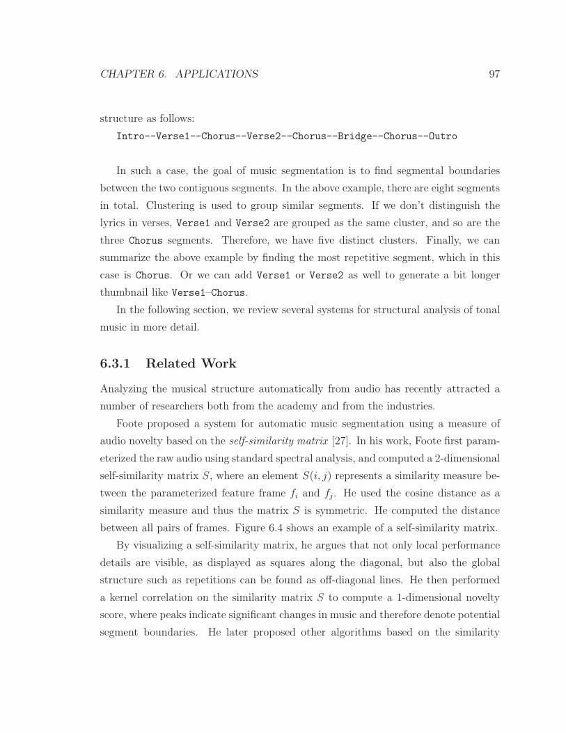
CHAPTER 6. APPLICATIONS 97
structure as follows:
Intro--Verse1--Chorus--Verse2--Chorus--Bridge--Chorus--Outro
In such a case, the goal of music segmentation is to find segmental boundaries
between the two contiguous segments. In the above example, there are eight segments
in total. Clustering is used to group similar segments. If we don’t distinguish the
lyrics in verses, Verse1 and Verse2 are grouped as the same cluster, and so are the
three Chorus segments. Therefore, we have five distinct clusters. Finally, we can
summarize the above example by finding the most repetitive segment, which in this
case is Chorus. Or we can add Verse1 or Verse2 as well to generate a bit longer
thumbnail like Verse1–Chorus.
In the following section, we review several systems for structural analysis of tonal
music in more detail.
6.3.1 Related Work
Analyzing the musical structure automatically from audio has recently attracted a
number of researchers both from the academy and from the industries.
Foote proposed a system for automatic music segmentation using a measure of
audio novelty based on the self-similarity matrix [27]. In his work, Foote first param-
eterized the raw audio using standard spectral analysis, and computed a 2-dimensional
self-similarity matrix S, where an element S(i, j) represents a similarity measure be-
tween the parameterized feature frame fi and fj. He used the cosine distance as a
similarity measure and thus the matrix S is symmetric. He computed the distance
between all pairs of frames. Figure 6.4 shows an example of a self-similarity matrix.
By visualizing a self-similarity matrix, he argues that not only local performance
details are visible, as displayed as squares along the diagonal, but also the global
structure such as repetitions can be found as off-diagonal lines. He then performed
a kernel correlation on the similarity matrix S to compute a 1-dimensional novelty
score, where peaks indicate significant changes in music and therefore denote potential
segment boundaries. He later proposed other algorithms based on the similarity

CHAPTER 6. APPLICATIONS 98
Figure 6.4: Self-similarity matrix of the first seconds from Bach’s Prelude No. 1 inC major performed by Gould (from Foote [28]).
matrix to automatically find musical structures using MFCCs [28]. Foote and Cooper
also used a self-similarity matrix to cluster the segments and then summarize music
[29, 19, 20].
Although their work made significant contributions to visualizing the musical
structure and to finding the segments, it is entirely dependent on the distance be-
tween individual low-level feature frames and thus fails to provide the relationships
between the musical structure and high-level musical attributes such as melody or
harmony, which is highly correlated with the structure.
Aucouturier and Sandler used a three-state HMM for music segmentation, where
each state corresponds to {silence}, {voice + accordion + accompaniment} and
{accordion + accompaniment} [1]. They trained the model on the sequence of fea-
ture vectors using the classic Baum-Welch algorithm to estimate the states’ output
distributions and state-transition probabilities. They then used Viterbi decoding to

CHAPTER 6. APPLICATIONS 99
find the most probable state path, which also unveils the musical structure.
Even though they use a statistical model to learn from the actual data the struc-
ture of music, it is based on the assumption that the “texture” or “polyphonic timbre”
represented by low-level features of one segment are different from those of other seg-
ments, which may not be always true. For example, in music with very homogeneous
instrumentation, such as piano solo, it is not likely that each section reveals distinct
texture. Furthermore, they also assumed the fixed number of states or clusters, which
is unknown.
Levy and Sandler addressed the problems of such unsupervised learning model
and proposed a semi-supervised approach to segmentation [63]. They argue a simple
division of a piece into two regions by a user — therefore called semi -supervising —
helps initialize the states of the HMMs.
Goodwin and Laroche proposed a dynamic programming (DP) approach to audio
segmentation and speech/music discrimination [35]. To this end, they first performed
linear discriminant analysis (LDA) to condition feature space in a way that the classes
— speech and music classes in their application — are maximally separable from each
other, and apply dynamic programming to identify data clusters. The strength in
their approach is that no prior information as to the number of clusters or states is
required: DP finds it automatically as it computes the minimum cost path in feature
space as shown in Figure 6.5.
All the aforementioned systems for structural analysis of music, whether they
use a novelty measure between feature frames or a machine learning model to find
the statistical properties within the clusters, depend on the (dis)similarity of low-level
features, which barely have anything to do with more musically meaningful properties.
In the next section, we present a novel approach to finding structural boundaries
in tonal music based on the sequence of chords and their time boundaries.

CHAPTER 6. APPLICATIONS 100
Figure 6.5: In dynamic programming, clustering in feature-space is done by findingthe optimal state-path based on a transition cost and a local cost. The dotted diagonalis the nominal feature path. A candidate cluster path is shown in solid line (fromGoodwin and Laroche [35]).
6.3.2 Proposed System
In tonal music, the tonality of a piece is very closely related with the cadence. Grove
Music Online3 defines cadence as follows:
Cadence: The conclusion to a phrase, movement or piece based on a recognizable
melodic formula, harmonic progression or dissonance resolution; the formula
on which such a conclusion is based. The cadence is the most effective way of
establishing or affirming the tonality of an entire work or the smallest section
thereof; it may be said to contain the essence of the melodic (including rhythmic)
and harmonic movement, hence of the musical language, that characterizes the
style to which it belongs.
As is defined above, if we can identify the cadences in tonal music, we can also
recognize the phrase or section boundaries since a cadence concludes a musical seg-
ment such as a phrase or movement. Furthermore, among many musical attributes,
analyzing harmonic progression is the most definitive and effective way of identifying
such cadences in tonal music. Therefore, we propose a system for finding structural
3http://www.grovemusic.com

CHAPTER 6. APPLICATIONS 101
boundaries in tonal music by recognizing the cadences from the key and chord pro-
gression. Figure 6.6 shows the overall procedure of the proposed system using the
HMMs described in Chapter 3 and in Chapter 4. Each step is explained in more
detail as follows:
1) Feature extraction: Tonal centroid feature is extracted from audio as de-
scribed in Section 3.2.3.
2) Key & Chord recognition: Using key-dependent HMMs described in Section
4.2, key and the chord sequence with time boundaries are estimated from the
feature vectors.
3) Harmonic-Beat detection: Most dominant length of the chord duration is
computed by performing an autocorrelation analysis on the chord sequence.
Because we are not interested in how but when the chord changes, we convert
the chord sequence to an impulse train and the autocorrelation analysis is done
on this impulse train. This process is explained in more detail in Section 6.3.3.
Computation of harmonic beat is important in computing the tonal tension
curve because it is impossible to define the length of cadential formulas without
knowing the duration.
4) Tonal tension curve generation: Based on the harmonic-beat and key in-
formation, one or more cadential formulas are first created. We can use, for
example, only a perfect authentic cadence (V-I), or a combination of a perfect
authentic cadence and a half cadence such as IV-V. Once we have defined a ca-
dential formula, we slide it through the estimated chord sequence and compute
the distance between the cadential formula and the chord sequence at the frame
level. For instance, assume that the estimated key was C major. Then if the
harmonic beat was 10-frames long and if we used a V-I cadence, then we have
a 20-frame long cadential formula whose first 10 frames are in G major chord
and the last 10 frames are in C major chord. Therefore, if there are phrases
that end with a V-I cadence, we’ll have very low distance at those locations,
indicating the potential phrase boundaries.

CHAPTER 6. APPLICATIONS 102
Musical Audio
Key & Chord
Recognition
Detection
Harmonic−Beat
Feature Extraction
Curve Generation
Tonal Tension
Cadence
Recognition
Boundary Selection
Strurtural Boundaries
Figure 6.6: The overview of structural segmentation system

CHAPTER 6. APPLICATIONS 103
5) Cadence recognition: Once we compute the tonal tension curve, we can
recognize potential cadences by finding the local minima in the curve. We can
do this either by setting some threshold value heuristically or by finding the
local valleys significantly lower than the neighboring points.
6) Boundary selection: Since step 5 can give false cadences as well, we need a
pruning technique to select only true cadences. We prune such false cadences
by finding the most dominant segment length as we did to detect the harmonic
beat in step 3. This pruning is based on the assumption that most tonal music,
particularly most pop music, has a fairly regular structure, and therefore most
segments or phrases in a piece of music have a length that are related to the
length of such a dominant, fundamental segment. Therefore, once we figure out
the length of the most dominant segment, we can get rid of false boundaries
using a simple correlation analysis.
6.3.3 Experimental Results
Segmentation
Figure 6.7 shows the frame-level chord recognition results obtained using key-dependent
HMMs. The model correctly estimated the key, which is the key of C major.
The frame-level recognition accuracy was about 88.06%. We can observe in Figure
6.7 that the chord changes at a very regular rate most of the times. We can find
the length of the most dominant chord duration, or harmonic beat, using a simple
autocorrelation analysis. In doing so, we first generate an impulse train that has ones
whenever chord changes and zeros otherwise. This is because we are not interested
in how but when the chord changes. Then we compute the autocorrelation of this
impulse train, which is shown in Figure 6.8.
We can see in Figure 6.8 that the peaks can be found at about every 11 frames.
We can choose the first significant peak as the fundamental period of the harmonic
beat. The next step is to generate a cadential formula. Among several cadential
formulas, we use the perfect cadence or V-I movement since it is the most frequently
used cadence in tonal music. In addition, we also use the half-cadence in IV-V motion

CHAPTER 6. APPLICATIONS 104
0 20 40 60 80 100 120 140
CC#D
EbEF
F#G
AbA
BbB
CmC#mDm
EbmEmFm
F#mGm
AbmAm
BbmBm
Time (seconds)
Cho
rd
Chord recognition results
recognitionground truth
Figure 6.7: Frame-level chord recognition results (The Beatles’ “No Reply”).
0 10 20 30 40 50 60 70 80 90 1000
0.2
0.4
0.6
0.8
1
Time lag (frames)
Autocorrelation
Figure 6.8: Normalized autocorrelation of an impulse train obtained from the chordsequence shown in Figure 6.7.

CHAPTER 6. APPLICATIONS 105
Chord
Cho
rd
Chord−to−chord distance matrix
C C#D D# E F F# GG# A A# BCmC#mDmD#mEmFmF#mGmG#mAmA#mBmC
C#D
D#EF
F#G
G#A
A#B
CmC#mDm
D#mEmFm
F#mGm
G#mAm
A#mBm
0
0.05
0.1
0.15
0.2
0.25
0.3
0.35
0.4
Figure 6.9: 24×24 distance matrix between 12 major/minor chords in tonal centroidspace. Related chords are indicated by off-diagonals in lighter colors (e.g. C-F, C-G,C-Cm, C-Am).
as an additional cadential formula since it is also frequently used, especially in rock
music.
We then compute the Euclidean distance between the pre-defined cadential for-
mula and the chord sequence, for each cadential formula, and multiply them to obtain
a combined tonal tension curve. In computing the distance, we use a lookup table of
24×24 matrix which contains every possible chord-to-chord distance for 24 chords–12
major and 12 minor chords. This table is pre-computed using the observation distri-
bution parameters learned from the data. Figure 6.9 shows a 24 × 24 chord distance
matrix.
Using such a matrix to compute the tonal tension curve has several advantages.
First of all, it is meaningless to use the chord names in computing the distance

CHAPTER 6. APPLICATIONS 106
because the distance in the chord name space does not necessarily correspond to the
distance between the chords in a perceptual or musical sense. We may use a circle of
fifths to put related chords to close to each other, but computing the distance would
still be completely heuristic. However, using the observation probability distribution
of a feature vector such as tonal centroid, which is learned from the data, we can
appropriately represent the chords in the feature space, and therefore can estimate
the more meaningful distance between the chords.
A second advantage of this approach is that related chords such as tonic-dominant
or relative major-minor are close to each other in the feature space, resulting in
small distance, as shown in Figure 6.9 by off-diagonal lines in lighter colors. This is
important because even when the chord recognition is incorrect, it is highly likely that
the mis-recognized chord is related and thus the actual distance would still remain
small. This adds more robustness to the segmentation algorithm.
Lastly, since all possible chord-to-chord distance is pre-computed, it is computa-
tionally very efficient using a table lookup method.
Using the distance matrix described above, we compute the tonal tension curve
by sliding the cadential formula through the chord sequence, computing the distance
at the frame rate. When we encounter a chord transition same as or similar to
one defined in cadential formulas, we have very low tension or dissonance resolution,
indicating a potential phrase boundary. Figure 6.10 shows the tonal tension curve
overlaid with the chord recognition results.
From Figure 6.10, we observe several notches where tonal tension is minimal,
indicating the potential cadences or boundaries. As mentioned above, however, it is
possible that some of them are false cadences, and therefore we need to select only
true ones by pruning. We prune false cadences by finding the most significant segment
length, in a manner similar to how we find the harmonic beat. Once we find the most
dominant segment length, we generate a periodic impulse train whose fundamental
period is equal to the dominant segment length. We then slide this impulse train
through the tonal tension curve and compute the inner product. The final structural
boundaries are defined where the inner product is the smallest, namely the total
tonal tension is minimal. Estimated boundaries shown in Figure 6.11 are close to
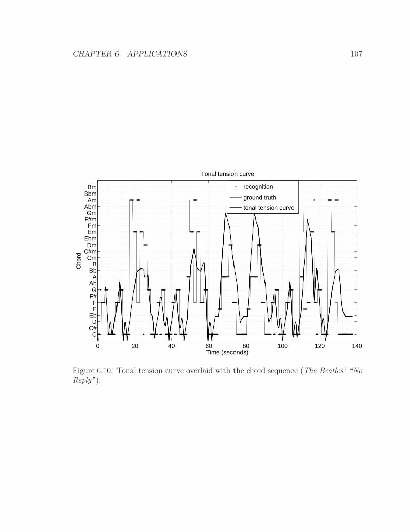
CHAPTER 6. APPLICATIONS 107
0 20 40 60 80 100 120 140
CC#D
EbEF
F#G
AbA
BbB
CmC#mDm
EbmEmFm
F#mGm
AbmAm
BbmBm
Time (seconds)
Cho
rd
Tonal tension curve
recognition
ground truth
tonal tension curve
Figure 6.10: Tonal tension curve overlaid with the chord sequence (The Beatles’ “NoReply”).

CHAPTER 6. APPLICATIONS 108
0 20 40 60 80 100 120 140
CC#D
EbEF
F#G
AbA
BbB
CmC#mDm
EbmEmFm
F#mGm
AbmAm
BbmBm
Time (seconds)
Cho
rdSegmentation result
recognized chordtonal tension curve
Figure 6.11: Final segmentation result. Estimated boundaries are shown in verticalsolid lines and true boundaries in dashed-dot lines (The Beatles’ “No Reply”).
true boundaries, except that there is another estimated boundary around 80 seconds
in the middle of the bridge section. We can eliminate this in the clustering stage, as
will be described shortly.
Clustering
Once we have found the structural boundaries, we can group the similar segments
into a cluster by computing the distance between a pair of segments for all possible
pairs. For example, we have nine segments in total in the above example. Since they
are of the same length, we can directly compute the frame-level distance between
a segment pair in the feature using the chord sequence. Figure 6.12 shows a 9×9
distance matrix of all segment pairs.
As is shown in Figure 6.12, the similar segments have smaller distance to each

CHAPTER 6. APPLICATIONS 109
Segment number
Seg
men
t num
ber
Segment−to−segment distance matrix
1 2 3 4 5 6 7 8 9
1
2
3
4
5
6
7
8
90.05
0.1
0.15
0.2
0.25
0.3
0.35
0.4
0.45
Figure 6.12: Distance matrix between segment pairs (The Beatles’ “No Reply”).
other and appear as lighter color in the distance matrix. We then normalize the
matrix and use a threshold value to determine if a segment pair is close enough
to be grouped as a cluster. The final clustering result is as follows: Cluster A:
{1,3,7}; Cluster B: {2,4,8}; Cluster C: {5,6}; Cluster D: {9}. If there are contiguous
segments in the same cluster, such as segments 5 and 6 in the example, it implies a
continuously repeating segment and thus we can group them into one segment. This
will remove an extra boundary in Figure 6.11 and will result in segmentation closer
to true segmentation,
Music Summarization
As has been described earlier, the most representative part in an entire piece of music
is often the most frequently repeating part, such as a chorus section. Therefore, once
we have found out the clustering information, we can easily summarize music simply
by finding the cluster with the largest number of segments, because the segments in
a cluster are similar to each other, or repetitive. So, in the above example, we can
choose either a segment in Cluster A or one in Cluster B, or both since the number
of repetitions is the same. Figure 6.13 illustrates the overall process of structural

CHAPTER 6. APPLICATIONS 110
Summarization oror
Segmentation
Clustering
Figure 6.13: Structural analysis: segmentation, clustering and summarization.
analysis.
6.4 Miscellaneous Applications
The applications described in the previous sections — cover song identification and
music segmentation/clustering/summarization — use the chord sequences as a front
end to the systems to perform these tasks. However, a sequence of chords and cor-
responding boundaries by themselves, although not 100% correct, provide invaluable
information to perform harmonic analysis of music. In addition, with the combination
of musical key, which is estimated using key-dependent models as explained in Chap-
ter 4, one can derive functional harmony in which each chord has a specific function
with regard to its tonal center such as tonic, dominant or subdominant and so on.
This will help many non-musicians or students without any formal music education
understand the harmonic structure of music.
Chords can also be used in melody extraction to reduce the search space when
estimating the pitch. This is because melody and chord are very closely related in
tonal music, and therefore a melody tone is usually one of the chord tones, assuming
enharmonic and octave equivalence. For example, if we know, at a certain time, that
the current chord is a C major triad, then we can have more confidence in pitch
classes such as C, E or G. Such melody-chord relationships can also be learned from
the data to build a statistical model.
CHAPTER 6. APPLICATIONS 111
In applications like music recommendation or playlist generation, a mood is one
of important criteria to find similarity or categorize in a collection of music. Mood is
a complex state of mind and in music, several attributes such as melody, key, tempo
or timbre contribute to defining the mood. We can infer simple relations like (fast
tempo, major key ↔ happy) or (slow tempo, minor key ↔ sad), for instance. We
believe harmonic progression also contributes significantly to building the mood in
music. For example, even when a piece is in a major key, a frequent usage of minor
chords can make it sound sad. The similar argument holds for a piece with a number
of major chords but in a minor key. Therefore, knowing the harmonic content and
its progression over time will help classify the mood in tonal music. Mood-specific
HMMs, where each HMM is trained on a specific mood as in key-dependent or genre-
specific HMMs, showed promising results in the Audio Music Mood Classification
competition in MIREX 2007.4
Audio mixing is another interesting and practical application where a chord se-
quence is very useful. When mixing several or more clips from different musical
sources, the process can’t be arbitrary: it is very important to preserve consistency
through a mixing process and placing the right chord at the right time is one of crit-
ical requirements to maintain such consistency. Furthermore, harmonic progression
tells the degree of closure or cadence via specific sequence of chord functions such
as dominant-tonic. Therefore, if we know the chord progression characteristic in the
clips to be mixed, it is possible to edit and arrange them in a harmonically pleasing
way.
6.5 Summary
In this chapter, we have demonstrated that a sequence of chords and chord time
boundaries provide useful information in applications such as cover song identification
and structural analysis.
In cover song finding, we use a pair of one-dimensional chord sequence as input
4http://www.music-ir.org/mirex2007/index.php/Audio Music MoodClassification

CHAPTER 6. APPLICATIONS 112
to the dynamic time warping algorithm to score an alignment between the two songs
abstracted through chord sequences. The rationale behind this idea was that har-
monic content would remain largely intact under various acoustical changes found
in different versions of cover songs. In computing the total cost, we not only used
optimal state alignment but also a transition cost from chord to chord to reflect the
theory of harmonic progression in Western tonal music. This increased the precision
of the system evaluated using a recall-precision test. The evaluations performed by
the author and by MIREX 2006 prove that the chord sequence is an efficient and
robust feature in cover song identification
We have presented a novel approach to structural analysis by recognizing cadences
in chord sequences. The hypothesis was, in tonal music, that a section such as a
phrase, chorus or verse ends on some sort of cadential movement in general. Therefore,
finding the cadences leads to finding the phrase boundaries. In doing so, we first detect
the harmonic beat or the rate at which the chord is most likely to change, and define
the cadential templates based on the key. We then slide these cadential templates
through the recognized chord sequence and compute the distance, resulting in the
tonal tension curve. When there are chord transitions the same as or similar to one
defined in cadential templates, tonal tension will be low, which indicates potential
phrase boundaries. False boundaries are removed using the dominant phrase length
to give final segmentation results.
After segmentation, we compute the distance between each pair of segments and
group those which are close to each other into a cluster. Finally, we summarize music
by selecting the segment(s) that are most often repeated.
We have also described several potential applications, including analysis of func-
tional harmony, melody extraction, mood classification and audio mixing, where har-
monic content can be directly or indirectly used.

Chapter 7
Conclusions and Future Directions
7.1 Summary of Contributions
In this dissertation, we have presented a unified system for chord transcription and
key extraction from audio. The main contribution of this work is its presentation of
a framework for acquiring a large amount of training data, via a nearly labor-free
process, that enables us to use a powerful supervised learning algorithm, leading to
state-of-the-art performance in both musical tasks.
The key idea in this approach is using symbolic music data. Symbolic music files
such as MIDI files contain noise-free information about pitch and duration of the
notes and therefore it is much easier and more robust to perform harmony analysis to
obtain the ground-truth data. In parallel, we synthesize the symbolic files to create
audio from which we extract the feature vectors. The acoustic feature vectors and the
chord labels are then in perfect alignment and we can use them to train the models
in a supervised way.
The labeled training data allow us to directly estimate the model parameters;
that is, we avoid the process of model initialization which is critical to accurately
estimate the parameters in unsupervised learning. We also avoid incorporating any
heuristics or musical knowledge that are required in many other key-finding or chord
recognition systems for parameter estimation; we just give the data and the models
will learn all the parameters.
113

CHAPTER 7. CONCLUSIONS AND FUTURE DIRECTIONS 114
We chose a first-order hidden Markov model for chord recognition and key es-
timation because of its abilities to describe temporal dynamics in observations, via
transition probabilities, which are very important in music in general, and in chord
progression in particular. The hidden state in the HMM represents a chord and is
modeled by a single, multivariate Gaussian (12-dimensional for chroma feature or
6-dimensional for tonal centroid feature). We defined 36 states or chords in an HMM,
including major, minor and diminished chords for each pitch class in a chromatic
scale. We treated seventh chords as their corresponding root triads and disregarded
augmented chords since they very rarely appear in Western tonal music. We allowed
all possible transitions from chord to chord, resulting in an ergodic HMM.
As feature vectors, we compared the conventional 12-dimensional chroma vectors
to the 6-dimensional tonal centroid vector. Chroma has been successfully used by
others in chord recognition and in key finding. Tonal centroid is computed by a linear
transformation from the chroma vector, and puts emphasis on important interval
relations such as fifths, major and minor thirds. The experiments showed that the
tonal centroid feature significantly outperformed the chroma feature.
After training the model with synthesized audio, we evaluated our system using
various kinds of musical audio and demonstrated that the models trained just on
synthesized audio perform very well on real recordings as well, in both musical tasks.
We also compared our data-driven model with a state-of-the-art knowledge-based
model to show that our model performs better than or comparable to the knowledge-
based model.
A large training data set enabled us to build richer models, and we extended our
HMM to be key-dependent as described in Section 4.2. The rational behind this idea
was a close relationship between key and chord in tonal music. If we know what
key a piece is in, recognizing chords is easier. We therefore built 24 key-dependent
HMMs, one for each key, using key information derived from the symbolic music files.
Given an acoustic input, our system performed feature analysis and a sequence of
observation became an input to the key-dependent HMMs. Using a Viterbi decoder,
we estimated the key by selecting the model with the maximum likelihood; at the
same time, we recognized frame-level chord sequence because it is the same as the

CHAPTER 7. CONCLUSIONS AND FUTURE DIRECTIONS 115
optimal state path in a selected key model. Experiments on real acoustic recordings
showed that a key-dependent model not only estimated the key of an input, but
also increased the chord recognition accuracy, yielding very promising results on both
musical tasks.
Based on the fact that each musical genre has chord progression characteristics of
its own, we also extended our basic model to build genre-specific models in Section
4.3. Although genre information is not explicitly encoded in symbolic music files,
it is not difficult to find symbolic music files categorized by genres. We therefore
built genre-specific HMMs, similar to key-dependent HMMs, resulting in improved
performance with much simpler models than a more complex, genre-independent
model. Experimental results showed that the performance is best when the model
and the unknown input are of the same kind, which supports our hypothesis on the
need for building genre-specific models. Furthermore, a selected genre model using
a maximum likelihood often gave a correct genre, suggesting the possibility of using
the model as a genre classifier.
We also introduced a hybrid model for chord recognition in Chapter 5. In the
hybrid model, we used powerful discriminative classifiers to compute the posterior
probabilities given the observation feature vector. To this end, we used support vector
machines (SVMs) which are widely used successfully in many other classification
problems, including several music applications. Experiments showed the proposed
discriminative approach using SVMs achieved the better performance when the same
amount of data (1/15 of the full set) is used to train both SVMs and Gaussian models.
Another principal contribution of this dissertation is the demonstration that a
harmonic description of music can be a compact, robust mid-level representation in
several potential applications as described in Chapter 6. These applications are very
important in music information retrieval because they allow efficient and effective
methods in search/retrieval. One such application is finding cover versions of an orig-
inal using the chord sequence as a front end to the system, as explained in Section
6.2. In order to identity cover songs, which can be acoustically very different from
the original because of changes in instrumentation, tempo, key and/or dynamics, we
need a robust representation that must remain largely invariant under such acoustical
CHAPTER 7. CONCLUSIONS AND FUTURE DIRECTIONS 116
transformations. Our hypothesis was that chord sequence is a robust mid-level repre-
sentation that undergoes only minor changes under such musical variations. We then
computed the optimal alignment of the original and cover song chord sequences using
dynamic time warping algorithm. The results showed that the chord sequence can
be successfully used to identify cover songs, proving our hypothesis. We also believe
that it is usable in finding musical similarity as well.
Harmonic description of tonal music, as represented by key and chords, is a fun-
damental attribute for music analysis as described in a number of treatises. Music
analysis often leads to finding a structure —i.e., searching for smaller building blocks
which all together form a whole piece. Therefore, we can use key and chords to
perform structural analysis of music, which leads to three closely related practical
applications, namely music segmentation, clustering and summarization.
In music segmentation, we tried to identify structural boundaries in musical audio.
We presented a novel approach to this problem in Section 6.3 by recognizing cadences
based on the fact that, in tonal music, a section usually ends with a cadence, which
is a specific harmonic motion (e.g., V-I movement in perfect cadence) characterized
by its key. To this end, we first extracted key and frame-level chords and defined
cadential templates based on the estimated key. We then located the positions where
such cadential movements are found by computing the tonal tension curve using the
pre-defined cadential templates and chord sequence. The valleys in the tonal tension
curve indicated potential cadences, namely structural boundaries. We then used a
pruning technique to remove false boundaries by finding the most dominant phrase
length.
Some sections in tonal music, particularly in popular music, share the same har-
monic content. For instance, the harmonic content of the first and the second verse
or that of chorus sections seldom changes. Therefore, we can group similar segments
into a cluster by finding harmonically similar segments. We computed segment-to-
segment distances at the chord level and grouped segments that are close enough to
each other to find a cluster. This clustering is useful in identifying repeating segments
such as chorus or verse, which also leads to another immediate application of music
summarization. Often the times, the most repeating section in music is also the most
CHAPTER 7. CONCLUSIONS AND FUTURE DIRECTIONS 117
remembered or representative section. Therefore, we could find a summary of mu-
sic, sometimes called an audio thumbnail, by recognizing the most repeating section
based on clustering information.
We also described other potential applications where harmonic descriptions are
valuable such as melody extraction, music recommendation, playlist generation, mood
classification or audio mixing.
We believe that the proposed system for chord recognition and key extraction
achieves state-of-the-art performance in both musical tasks. Although the proposed
hidden Markov models could successfully learn the first-order (i.e., from the current
to the next) chord transition probability distributions from the data, most tonal music
employs higher-order chord progressions, which leads to a direction for further work.
7.2 Higher-Order HMM
7.2.1 Introduction
The HMMs described in Chapter 3 and in Chapter 4 are based on the first-order
Markov process; that is, the current state qt (chord) is only dependent on the prede-
cessor state qt−1 (chord), namely
P (qt = Sj |qt−1 = Si, qt−2 = Sk, · · · ) = P (qt = Sj|qt−1 = Si). (7.1)
Therefore, given the predecessor state qt−1 (chord), knowing the previous state(s)
qt−2, qt−3, · · · (chords) has no effect in predicting the current state qt (chord). How-
ever, this first-order property does not hold in music or in chord progression in partic-
ular. For example, a popular 12-bar blues1 has a chord progression of {I-I-I-I-IV-IV-
I-I-V-V(IV)-I-I} [43]. Such higher-order progression is also common in tonal music
in general. For instance, {ii-V-I} or {iv-V-i} movement are most common cadential
formulas [46].
1Although it is originated in blues music, the 12-bar blues progression is one of the mostwidely used chord progressions in popular music in general.

CHAPTER 7. CONCLUSIONS AND FUTURE DIRECTIONS 118
Therefore, if we know two or more preceding chords in tonal music, it is very likely
that we can decide which chord to follow with more confidence. In fact, high-order
HMMs perform better and thus have been successfully used in Natural Language
Processing (NLP) [65, 22, 10, 34]. It is straightforward to solve the three basic
problems of a high-order HMM2 based on the first-order HMM. Interested readers
are encouraged to read du Preez [23].
When applying high-order HMMs to chord recognition, however, we encounter a
few problems. First, we can’t recognize chords at the frame-rate any more because
high-order chord transitions are not likely to happen at the frame rate; in other words,
it is very unlikely that the chord changes at one frame and changes again at the very
next frame. This in turn means that we can never model high-order chord transition
characteristics like {ii-V-I}, for example, at the frame-level. Therefore, in order to
use higher-order HMMs, we need to perform higher-level segmentation analysis than
at the frame-level.
One possible solution to this problem is to use beat-synchronous analysis as
done by Bello and Pickens in chord recognition [8]. Although they didn’t do beat-
synchronous analysis for modeling high-order chord progressions, we may be able to
learn high-order chord transitions at the beat-level. In order to be more precise, how-
ever, we need to find out the harmonic beat rather than the rhythmic beat since the
two can be different in general. We proposed an algorithm to compute the harmonic
beat in Section 6.3.2 which can be used for harmonic beat-level analysis.
Another problem in high-order modeling is data sparsity. Because we increase the
order of state transitions, the possible number of transitions increases exponentially,
assuming an ergodic model3 Therefore, if we had 36 × 36 = 1, 296 possible chord-to-
chord transitions with 36 different chords, in a 2nd-order HMM, we have 36×36×36 =
46, 656 possible transitions. This means we need even more data to appropriately fill
this 3-dimensional matrix; in fact, even with a lot more data, most elements in the
matrix will be zero. This leads to a serious overfitting problem since the model
can never generalize to unseen input sequences. And yet this is in the case of only
2Refer to Section A.4 in Appendix A3In an ergodic model, every state-to-state transition is possible.
CHAPTER 7. CONCLUSIONS AND FUTURE DIRECTIONS 119
2nd-order model.
This sparse-data problem becomes even more serious when we analyze audio at
a higher level than at the frame-level such as beat-synchronous level, because the
number of training samples becomes much less. To make this more concrete, we
could train the 2nd-order model to learn the 2nd-order transition probabilities using
the beat-level training data which contain more than 223,000 samples. The result
was less than 20% of the matrix elements were nonzero; in other words, more than
80% of all possible chord-to-chord-to-chord transitions never happened!
The data sparsity is a central issue in language modeling as well. Researchers
therefore proposed several smoothing algorithms to alleviate the sparsity problem
[41, 42, 18, 45]. In smoothing algorithms, some probability is taken away from some
occurrences because occurrences which appear only one time are usually greatly over-
estimated [34]. By taking some probability from some words and redistributing it to
other words, zero probabilities can be avoided.
We believe we can apply these smoothing techniques widely used in language
modeling to our application although the language context and the musical context
are different from each other.
7.2.2 Preliminary Results and Discussions
We experimented with the 2nd-order HMM which was trained on beat-synchronous
data. For training data, we didn’t perform beat-analysis on audio because Temper-
ley’s Melisma Music Analyzer also gives beat information [95]. For test audio. we
used the beat-detection algorithm by Ellis [26]. The feature frames in a beat seg-
ment was averaged to give one feature vector per beat. Table 7.1 shows the chord
recognition results with the song No Reply by the Beatles.
As shown in Table 7.1, the accuracy is highest with the 1st-order HMM trained on
the frame-level data, followed by the 1st-order HMM trained on the beat-synchronous
data. The proposed 2nd-order model trained on the beat-level data performed worse
than the 1st-order models. One thing that is noticeable is a significant performance
increase in the 2nd-order HMM when the data is smoothed (from 67% to 84%). This

CHAPTER 7. CONCLUSIONS AND FUTURE DIRECTIONS 120
Table 7.1: Test results on 2nd-order HMM (% correct)Analysis level
Model Frame Beat-synchronous1st-order 86.45 84.49
2nd-order (w/o smoothing) N/A 66.992nd-order (w/ smoothing) N/A 83.51
supports the idea that the smoothing techniques for language modeling are applicable
to music application.
There are a few possible explanations why the 2nd-order model performs no better
than the 1st-order models. First, the beat-analysis algorithm must be consistent
between the training and the test data, which isn’t the case in our experiments.
While beat information in the training data is directly extracted from the symbolic
data, not from the synthesized audio, we detect the beat from audio for the test data.
We plan to perform beat-analysis on the synthesize training audio using the same
beat-detection algorithm used for the test data.
Secondly, we may need more data to estimate the model parameters more accu-
rately. As mentioned earlier, the number of parameters to be estimated grows expo-
nentially as the order of Markov process in HMMs increases, although a smoothing
technique helps avoid overfitting problems.
Finally, we are not sure of the applicability of the smoothing techniques used in
language modeling to music application, especially in chord recognition. Although
the fundamental idea in smoothing —i.e. redistributing the probabilities from rare
occurrences to others to avoid zero probabilities — may also hold in chord progression
modeling, the word space is far bigger than the chord space (thousands of words vs.
36 chords), and thus the same smoothing techniques may not be appropriate. This
may require modifying the smoothing techniques to make them more suitable for
chord progression modeling.

CHAPTER 7. CONCLUSIONS AND FUTURE DIRECTIONS 121
7.3 Musical Expectation
7.3.1 Introduction
As has been pointed out several times in this dissertation, harmonic description of
tonal music, represented by key and chord names (and their onset/offset time), is a
powerful attribute to describe musical semantics (e.g., expectation, emotion/mood,
storytelling, etc.). In particular, as we listen to music, we constantly build some
sort of expectations — consciously or unconsciously — and our emotions, to a great
degree, are governed by their realizations or violations.
Music listening involves continuous interactions between the stimulus, namely the
listener’s perception, and mental processes. In doing so, the listener builds “tenden-
cies” to respond to the musical stimuli. According to Meyer,
. . . The tendency to respond becomes more conscious where in-
hibition of some sort is present, when the normal course of the
reaction pattern is disturbed or its final completion is inhibited.
Such conscious and self-conscious tendencies are often thought of
and referred to as “expectations” [66].
The musical expectations can be formed by melody, harmony, rhythm or by a
combination of such attributes. However, in Western tonal music, expectations are
particularly pronounced in the use of harmony as the most pervasive forms of music
employ a small set of chords in highly constrained ways [9]. Bharucha and Stoeckig
explored the cognitive processes underlying musical expectation by reaction time in
a priming paradigm, and observed that a harmonic context primes the processing of
chords related to the context, relative to chords unrelated to the context. They also
proposed a spreading activation network model of the representation and processing
of harmony, and proved the hypotheses using a set of experiments for chord priming.
Povel also investigated on musical expectations evoked by a sequence of chords in
exploring the elementary harmonic force present in tonal music, based on the similar
experiments done by Bharucha and Stoeckig [85].

CHAPTER 7. CONCLUSIONS AND FUTURE DIRECTIONS 122
7.3.2 Modeling Musical Expectation
These close relationships between harmony and musical expectations found in the
literature suggest that we can induce the level and the type of expectations from
chord progression or a sequence of chords. For example, if our chord recognition
system tells a chord sequence like {C-d-G}, then we can say there is a very strong
expectation that a C major chord will follow. If a C major chord follows, as expected,
then our expectation is realized. If the next chord is instead a B♭ major for example,
however, then we can say that our expectation is violated. This concept of implication-
realization model in the context of melody expectation was studied by Narmour
[70, 71].
Leistikow proposed a probabilistic framework to model musical expectations [62].
In his thesis, he presented a dynamic Bayesian inference engine to model an array of
cognitive tasks performed by a listener when presented with musical sounds. He used
a set of musical rules learned from musical corpora to predict upcoming notes and
measured the surprise associated with the observed realizations.
As Leistikow suggested that his expectation models can be seamlessly integrated
into probabilistic models that use audio signal features as input, we hope in the fu-
ture to develop such a framework for modeling musical expectations from audio using
our model to provide higher-level symbolic attributes — musical key and chords —
extracted from audio. In addition, we can build a hierarchical model such as one de-
scribed by Leistikow in which several musical attributes are mutually informative [62].
Although there are many more variables defined in his model, including meter, beat,
duration, bar, harmony, and the observation is a (symbolic) musical note, we can
build a similar hierarchical model with a reduced set of variables — that is, key, har-
mony and beat — and with the chroma or tonal centroid feature as observations. Our
system doesn’t have a beat-detection algorithm, but we believe it is needed because
beat information is directly or indirectly related to many other musical properties.
Once we build such a hierarchical model, the evaluation of expectation realiza-
tion/violation can be performed following these steps:
1. Estimate the prior distributions and the transition distributions from the labeled

CHAPTER 7. CONCLUSIONS AND FUTURE DIRECTIONS 123
training data as we do in our proposed system (assuming we perform beat-
synchronous analysis).
2. Perform chord recognition and key extraction given an input audio. We may also
consider local key-finding to examine more localized key-harmony relationships.
3. Compute a one-step observation prediction given as
P (Xi+1|x1:i) =∑
KCBi,KCBi+1
P (KCBi, KCBi+1, Xi+1|x1:i), (7.2)
where Ki, Ci, Bi, Xi denote key, chord, beat and observation at time i.
4. Compute the violation or surprisal of that observation by evaluating
Surprisal(xi+1|xi) = − log2 P (Xi+1 = xi+1|x1:i). (7.3)
We can compute the quantities in Step 3 and 4 using the directed acyclic graph
(DAG) for a hierarchical model proposed by Leistikow [62].
7.4 Final Remarks
It is our hope that the framework for extracting harmonic content from musical audio
will make a significant contribution to the music information retrieval community in
general and to those who try to apply machine learning techniques to solve music-
related problems in particular. With our initial phase of research concluded, we wish
to continue to work on more difficult, but even more interesting problems, such as
those suggested in the previous sections, in the future.

Appendix A
Hidden Markov Model 1
A.1 Discrete Markov Process
Figure A.1 illustrates a Markov chain with four states that may be described at any
time as being in one of N distinct states, S1, S2, · · · , SN (N = 4 in this example). If
we denote the time instants associated with state changes as t = 1, 2, · · · , and the
actual state at time t as qt, we can fully describe the behavior of such system by
specifying the current state at time t and the previous states at time t− 1, t− 2, · · · .
For the special case of a discrete, first-order, Markov chain, this probabilistic
description simplifies to just the current and the preceding state, i.e.,
P (qt = Sj |qt−1 = Si, qt−2 = Sk, · · · ) = P (qt = Sj|qt−1 = Si). (A.1)
Furthermore, only considering those process where the right-hand side of Equation
A.1 is independent of time leads to a set of state transition probabilities aij of the
form
aij = P (qt = Sj|qt−1 = Si), 1 ≤ i, j ≤ N (A.2)
1This appendix is based on Rabiner [86] and Rabiner and Juang [87]
124

APPENDIX A. HIDDEN MARKOV MODEL 125
S4
S1 S2
S3
Figure A.1: A Markov chain with 4 states (labeled S1 to S4) with all possible statetransitions.
with the following properties:
aij ≥ 0 (A.3a)N
∑
j=1
aij = 1. (A.3b)
The above Markov process may be called an observable Markov model since the
output of the process is the set of states at each time, where each state corresponds
to a physical (and thus observable) event.
For example, let’s consider a simple three-state Markov model of the weather,
where the weather is observed, once a day, as being one of the following:
State 1 (S1): rain
State 2 (S2): cloudy
State 3 (S3): sunny.
We assume that the weather on day t undergoes a change of a state based on the

APPENDIX A. HIDDEN MARKOV MODEL 126
state transition probability matrix A given by
A = {aij} =
0.4 0.3 0.3
0.2 0.6 0.2
0.1 0.1 0.8
. (A.4)
We can then ask a question such as: given that the weather on day 1 (t = 1)
is sunny (S3 = 3), what is the probability that the weather for the next three days
will be “sun-sun-cloudy-rain-rain”? Stated more formally, we define the observation
sequence O as O = {S3, S3, S2, S1, S1} at t = 1, 2, · · · , 5, respectively, and we wish
to compute the probability of O, given the above model. This probability can be
expressed and evaluated as
P (O|Model) = P (S3, S3, S2, S1, S1|Model)
= P (S3)P (S3|S3)P (S2|S3)P (S1|S2)P (S1|S1)
= π3 · a33 · a32 · a21 · a11
= 1 · 0.8 · 0.1 · 0.2 · 0.4
= 0.0064 (A.5)
where we use the notation
πi = P (q1 = Si), 1 ≤ i ≤ N (A.6)
to denote the initial state probabilities.
A.2 Extension to Hidden Markov Models
In the Markov model described above, each state (weather on a day) corresponds to
an observable (physical) event (rain, cloudy or sunny). This model is too restrictive
to be applicable to many problems since we may not be able to directly observe the
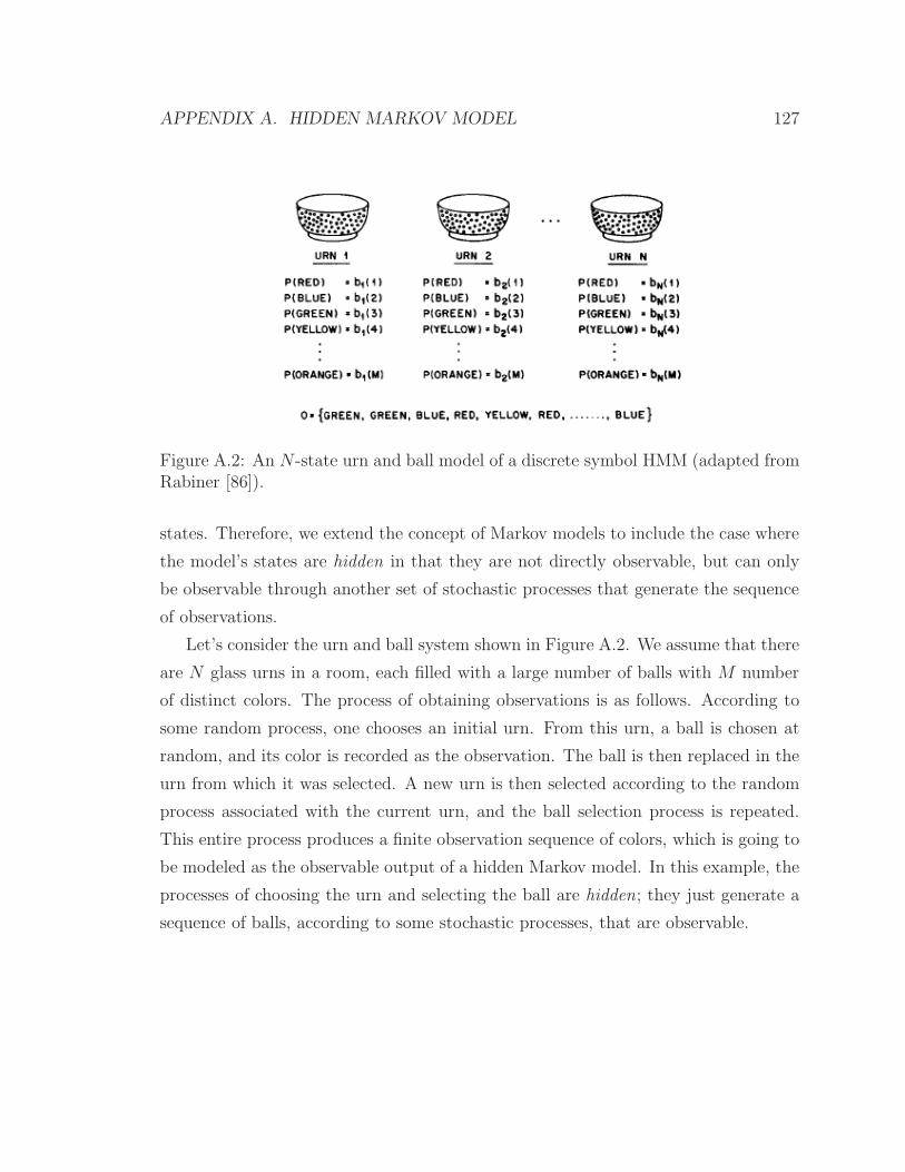
APPENDIX A. HIDDEN MARKOV MODEL 127
Figure A.2: An N -state urn and ball model of a discrete symbol HMM (adapted fromRabiner [86]).
states. Therefore, we extend the concept of Markov models to include the case where
the model’s states are hidden in that they are not directly observable, but can only
be observable through another set of stochastic processes that generate the sequence
of observations.
Let’s consider the urn and ball system shown in Figure A.2. We assume that there
are N glass urns in a room, each filled with a large number of balls with M number
of distinct colors. The process of obtaining observations is as follows. According to
some random process, one chooses an initial urn. From this urn, a ball is chosen at
random, and its color is recorded as the observation. The ball is then replaced in the
urn from which it was selected. A new urn is then selected according to the random
process associated with the current urn, and the ball selection process is repeated.
This entire process produces a finite observation sequence of colors, which is going to
be modeled as the observable output of a hidden Markov model. In this example, the
processes of choosing the urn and selecting the ball are hidden; they just generate a
sequence of balls, according to some stochastic processes, that are observable.

APPENDIX A. HIDDEN MARKOV MODEL 128
A.3 Elements of an HMM
From the above example, we now formally define the elements of an HMM. An HMM
is characterized by the following:
1) N , the number of states in the model. Although the states are hidden in HMMs,
there is often physical significance in the states of the model. In the above urn
and ball example, the states corresponded to the urns. The states in general are
interconnected in such a way that any state can be reached from any other state;
however, it is sometimes more practical and appropriate to put some restrictions
on state transitions. We denote the individual states as S = {S1, S2, · · · , SN},
and the state at time t as qt.
2) M , the number of distinct observation symbols per state. The observation
symbols correspond to the physical output of the system to be modeled. In
the ball and urn example, they were the colors of the balls. We denote the
individual symbols as V = {v1, v2, · · · , vM}.
3) The state transition probability distribution A = {aij} where
aij = P (qt+1 = Sj |qt = Si), 1 ≤ i, j ≤ N, (A.7)
with the properties given in Equation A.3.
4) The observation probability distribution in state j, B = {bj(k)}, where
bj(k) = P (vk at t|qt = Sj), 1 ≤ j ≤ N, 1 ≤ k ≤M. (A.8)
5) The initial state distribution π = {πi} where
πi = P (q1 = Si), 1 ≤ i ≤ N. (A.9)
Given appropriate values of N,M,A,B, and π, the HMM can be used to generate
an observation sequence
APPENDIX A. HIDDEN MARKOV MODEL 129
O = O1O2 · · ·OT , (A.10)
where each observation Ot is one of the symbols from V , and T is the number of
observations in the sequence, as follows:
1) Choose an initial state q1 = Si according to the initial state distribution π.
2) Set t = 1.
3) Choose Ot = vk according to the symbol probability distribution in state Si,
i.e., bi(k).
4) Transit to a new state qt+1 = Sj according to the state transition probability
distribution for state Si, i.e., aij .
5) Set t = t+ 1; return to step 3) if t < T ; otherwise terminate the procedure.
We can see from the above discussion that an HMM is completely characterized
by the specification of two model parameters (N and M), observation symbols and
the three probability measures A,B, and π. For convenience, we use the compact
notation
λ = (A,B, π) (A.11)
to indicate the complete parameter set of the model.
A.4 The Three Fundamental Problems of an HMM
Given the form of HMM described in the previous section, there are three basic
problems that must be solved for the model to be useful in real-world applications.
These problems are:

APPENDIX A. HIDDEN MARKOV MODEL 130
Problem 1: Given the observation sequence O = O1O2 · · ·OT and a model
λ = (A,B, π), how do we efficiently compute P (O|λ), the probability of the
observation sequence, given the model?
Problem 2: Given the observation sequence O = O1O2 · · ·OT and a model
λ, how do we choose a corresponding state sequence Q = q1q2 · · · qT which is
optimal in some meaningful sense (i.e., best “explains” the observations)?
Problem 3: How do we adjust the model parameters λ = (A,B, π) to maximize
P (O|λ)?
Problem 1 is the evaluation problem; i.e., given the observation sequence and a
model, how do we compute the probability that the model produced the observation
sequence. This is extremely useful when we try to choose among several competing
models by allowing us to select the model with the highest probability.
Problem 2 is the one where we try to uncover the hidden part of the model, namely
the “correct” state path. However, there is no “correct” state sequence except for
the degenerate models, and therefore in practical applications, we usually use an
optimality criterion to solve the problem as best as possible.
Problem 3 is the one in which we attempt to optimize the model parameters in
order to best explain how a given observation sequence is generated. We refer to this
procedure as “training” the HMM and call the observation sequence used to adjust
the model parameters a training sequence. The training problem is very important for
most applications because it allows us to build best models for real-world phenomena.
A.4.1 Solution to Problem 1
We wish to compute P (O|λ), the probability of the observation sequence O = O1O2 · · ·OT ,
given the model λ. Let’s consider a state sequence
Q = q1q2 · · · qT (A.12)

APPENDIX A. HIDDEN MARKOV MODEL 131
then the probability of the observation sequence O for the state sequence Q of Equa-
tion A.12 is
P (O|Q, λ) =
T∏
t=1
P (Ot|qt, λ) (A.13a)
= bq1(O1)bq2
(O2) · · · bqT(OT ), (A.13b)
where we have assumed statistical independence of observations.
The probability of such a state sequence Q can be written as
P (Q|λ) = πq1aq1q2
aq2q3· · ·aqT−1qT
. (A.14)
The joint probability of O and Q is simply the product of the above two terms,
i.e.,
P (O,Q|λ) = P (O|Q, λ)P (Q|λ). (A.15)
Therefore, the probability of O given the model λ is obtained by summing this joint
probability over all possible state sequences q giving
P (O|λ) =∑
all Q
P (O|Q, λ)P (Q|λ) (A.16a)
=∑
q1,q2,··· ,qT
πq1bq1
(O1)aq1q2bq2
(O2) · · ·aqT−1qTbqT
(OT ). (A.16b)
The direct calculation of P (O|λ) following Equation A.16, however, involves on
the order of 2T · NT calculations and is computationally infeasible, even for small
values of N and T ; e.g., for N = 5 (states), T = 100 (observations), there are on the
order of 2 · 100 · 5100 ≈ 1072 computations! We can more efficiently solve this problem
using a procedure called a Forward-Backward algorithm.

APPENDIX A. HIDDEN MARKOV MODEL 132
Let’s consider the forward variable αt(i) defined as
αt(i) = P (O1O2 · · ·Ot, qt = Si|λ), (A.17)
i.e., the probability of the partial observation sequence O1O2 · · ·Ot until time t and
state Si at time t, given the model λ. We then can solve for αt(i) inductively, following
these steps:
1) Initialization:
α1(i) = πibi(O1), 1 ≤ i ≤ N. (A.18)
2) Induction:
αt+1(j) =
[
N∑
i=1
αt(i)aij
]
bj(Ot+1), 1 ≤ t ≤ T − 1, 1 ≤ j ≤ N. (A.19)
3) Termination:
P (O|λ) =
N∑
i=1
αT (i). (A.20)
In a similar manner, we can define a backward variable βt(i) as
βt(i) = P (Ot+1Ot+2 · · ·OT |qt = Si, λ), (A.21)
i.e., the probability of the partial observation sequence from t+1 to the end, given
state Si at time t and the model λ. Using this Forward-Backward algorithm2, we see
that the calculation of P (O|λ) requires on the order of N2T calculations, compared
with 2TNT as required by the direct calculation. For N = 5 and T = 100, this is
about 3000 computations versus 1072, a savings of about 69 orders of magnitude.
2In order to solve Problem 1, we only need the forward or backward part of the forward-backward procedure, but both procedures are required to solve Problem 3.

APPENDIX A. HIDDEN MARKOV MODEL 133
A.4.2 Solution to Problem 2
While there exists an exact solution to Problem 1, there are several possible ways to
solve Problem 2, i.e., finding the “optimal” state sequence associated with the given
observation sequence. Therefore, the solution may vary according to what optimality
criterion is used. One of such optimality criteria that are mostly widely used is to
find the single best state sequence or path to maximize P (Q|O, λ) which is equivalent
to maximizing P (Q,O|λ). A formal technique for finding this single optimal state
sequence exists, based on dynamic programming methods, and is called the Viterbi
algorithm.
We wish to find the single best state sequence, Q = q1q2 · · · qT , given the observa-
tion sequence O = O1O2 · · ·OT and the model λ. Let’s define the quantity
δt(i) = maxq1,q2,···qT
P (q1q2 · · · qt = i, O1O2 · · ·Ot|λ); (A.22)
i.e., δt(i) is the best score (highest probability) along a single path, at time t, which
accounts for the first t observations and ends in state Si. By induction we have
δt+1(j) =[
maxiδt(i)aij
]
· bj(Ot+1). (A.23)
In order to retrieve the state sequence, we need to keep track of the argument
which maximize Equation A.23, for each t and j. We do this via the array ψt(j)
which holds state information. The complete procedure can be explained as follows:
1) Initialization:
δ1(i) = πibi(O1), 1 ≤ i ≤ N (A.24a)
ψ1(i) = 0. (A.24b)
2) Recursion:
δt(j) = max1≤i≤N
[δt−1(i)aij ] bj(Ot), 2 ≤ t ≤ T, 1 ≤ j ≤ N (A.25a)
ψt(j) = argmax1≤i≤N
δt−1(i)aij , 2 ≤ t ≤ T, 1 ≤ j ≤ N (A.25b)

APPENDIX A. HIDDEN MARKOV MODEL 134
3) Termination:
p∗ = max1≤i≤N
δT (i) (A.26a)
q∗T = argmax1≤i≤N
δT (i). (A.26b)
4) Path (state sequence) backtracking:
q∗t = ψt+1(q∗t+1), t = T − 1, T − 2, · · · , 1. (A.27)
As can be shown in the above procedure, the Viterbi algorithm is similar in imple-
mentation, except for the backtracking step, to the forward calculation of Equation
A.18–A.20.
A.4.3 Solution to Problem 3
The third, and by far the most difficult, problem of HMMs is to adjust the model
parameters (A,B, π) to maximize the probability of the observation sequence given
the model, and there is no analytical solution to this problem. In fact, given any
finite training sequence, there is no optimal way of estimating the model parame-
ters. However, we can choose λ = (A,B, π) such that P (O|λ) is locally maximized
using an iterative approach such as the Baum-Welch method, also known as the EM
(Expectation-Modification) algorithm.
Let’s first define ξt(i, j), the probability of being in state Si at time t and in state
Sj at time t+ 1, given the model and the observation sequence, i.e.,
ξt(i, j) = P (qt = Si, qt+1 = Sj|O, λ). (A.28)
Using the definitions of the forward and backward variables in Equation A.17 and

APPENDIX A. HIDDEN MARKOV MODEL 135
A.21, respectively, we can rewrite ξt(i, j), using Bayes’ rule, in the form
ξ =αt(i)aijbj(Ot+1)βt+1(j)
P (O|λ)
=αt(i)aijbj(Ot+1)βt+1(j)
N∑
i=1
N∑
j=1
αt(i)aijbj(Ot+1)βt+1(j)
. (A.29)
If we define another variable γt(i), the probability of being in state Si at time t,
given the model and the observation sequence, as
γt(i) =αt(i)βt(i)
P (O|λ)=
αt(i)βt(i)N
∑
i=1
αt(i)βt(i)
(A.30)
we can relate γt(i) to ξt(i, j) by summing over j, giving
γt(i) =N
∑
j=1
ξt(i, j). (A.31)
If we sum this quantity over time t, we obtain the expected number of times that
state Si is visited, or equivalently, the expected number of transitions made from
state Si, excluding t = T for termination. Similarly, summation of ξt(i, j) over t
(from t = 1 to t = T − 1) gives the expected number of transitions from state Si to
state Sj, i.e.,
T−1∑
t=1
γt(i) = expected number of transitions from Si (A.32a)
T−1∑
t=1
ξt(i) = expected number of transitions from Si to Sj (A.32b)
Using the above formulas and definitions, we can give a method of re-estimating
the parameters of an HMM. A set of reasonable re-estimation formulas for π,A and

APPENDIX A. HIDDEN MARKOV MODEL 136
B are
πi = expected frequency (number of times) in state Si at time (t = 1)
= γ1(i) (A.33a)
aij =expected number of transitions from state Si to state Sj
expected number of transitions from state Si
=
T−1∑
t=1
ξt(i, j)
T−1∑
t=1
γt(i)
(A.33b)
bj(k) =expected number of times in state Sj and observing symbol vk
expected number of times in state Sj
=
T∑
t=1
s.t.Ot=vk
γt(j)
T∑
t=1
γt(j)
. (A.33c)
The above formulas allow us to recursively re-estimate the model parameters λ =
(A,B, π), as determined from the left-hand sides of Equation A.33 using the current
model λ = (A,B, π) on the right-hand sides. Baum and his colleagues [6, 3] have
proven that the re-estimated model λ is always equally likely as or more likely than
the current model λ in the sense that P (O|λ) ≥ P (O|λ); i.e., a new model λ is more
likely to have produced the observation sequence.
Therefore, if we iteratively use λ in place of λ to estimate new model parameters,
we can improve the likelihood of the observation sequence being generated by the
model until convergence. The final result of this re-estimation procedure is called
a maximum likelihood estimate of the HMM. It should be noted, however, that the
forward-backward algorithm leads to local maxima only, and thus the initialization
of the model is crucial in many real-world applications.

Bibliography
[1] Jean-Julien Aucouturier and Mark Sandler. Segmentation of musical signals
using hidden markov models. In Proceedings of the Audio Engineering Society,
2001.
[2] Ricard Baeza-Yates and Berthier Ribeiro-Neto. Modern Information Retrieval.
Addison-Wesley, New York, 1999.
[3] J. K. Baker. The dragon system — an overview. IEEE Transactions on Acous-
tics and Speech Signal Processing, 23(1):24–29, 1975.
[4] Roberto Basili, Alfredo Serafini, and Armando Stellato. Classification of mu-
sical genre: a machine learning approach. In Proceedings of the International
Conference on Music Information Retrieval, 2004.
[5] Roberto Basili, Alfredo Serafini, and Armando Stellato. An investigation of
feature models for music genre classification using the support vector classifier.
In Proceedings of the International Conference on Music Information Retrieval,
2005.
[6] L. E. Baum and G. R. Sell. Growth functions for transformations on manifolds.
Pacific Journal of Math, 27(2):211–227, 1968.
[7] Juan P. Bello. Audio-based cover song retrieval using approximate chord se-
quences: Testing shifts, gaps, swaps and beats. In Proceedings of the Interna-
tional Conference on Music Information Retrieval, Vienna, Austria, 2007.
137

BIBLIOGRAPHY 138
[8] Juan P. Bello and Jeremy Pickens. A robust mid-level representation for har-
monic content in music signals. In Proceedings of the International Conference
on Music Information Retrieval, London, UK, 2005.
[9] Jamshed Jay Bharucha and Keiko Stoeckig. Reaction time and musical ex-
pectancy: Priming of chords. Journal of Experimental Psychology: Human
Perception and Performance, 12(4):403–410, 1986.
[10] Thorsten Brants. TnT — a statistical part-of-speech tagger. In Proceedings of
the 6th Applied Natural Language Processing Conference, Seattle, WA, 2000.
[11] Judith C. Brown. Calculation of a constant-Q spectral transform. Journal of
the Acoustical Society of America, 89(1):425–434, 1990.
[12] Giordano Cabral, Francois Pachet, and Jean-Pierre Briot. Automatic x tra-
ditional descriptor extraction: The case of chord recognition. In Proceedings
of the International Conference on Music Information Retrieval, London, UK,
2005.
[13] Giordano Cabral, Francois Pachet, and Jean-Pierre Briot. Recognizing chords
with EDS: Part one. In Computer Music Modeling and Retrieval (CMMR
2005), Lecture Notes in Computer Science Series, pages 185–195. Springer-
Verlag, 2006.
[14] Wei Chai and Barry Vercoe. Detection of key change in classical piano music.
In Proceedings of the International Conference on Music Information Retrieval,
2005.
[15] Elaine Chew and Yun-Ching Chen. Real-time pitch spelling using the spiral
array. Computer Music Journal, 29(2):61–76, 2005.
[16] Ching-Hua Chuan and Elaine Chew. Fuzzy analysis in pitch class determination
for polyphonic audio key finding. In Proceedings of the International Conference
on Music Information Retrieval, London, UK, 2005.

BIBLIOGRAPHY 139
[17] Ching-Hua Chuan and Elaine Chew. Polyphonic audio key finding using the
spiral array ceg algorithm. In Proceedings of IEEE International Conference on
Multimedia and Expo, 2005.
[18] Kenneth W. Church and William A. Gale. A comparison of the enhanced good-
turing and deleted estimation methods for estimating probabilities of english
bigrams. Computer Speech and Language, 5:19–54, 1991.
[19] Matthew Cooper and Jonathan Foote. Automatic music summarization via
similarity analysis. In Proceedings of the International Conference on Music
Information Retrieval, Paris, France, 2002.
[20] Matthew Cooper and Jonathan Foote. Summarizing popular music via struc-
tural similarity analysis. In Proceedings of IEEE Workshop on Applications of
Signal Processing to Audio and Acoustics, New Paltz, NY, 2003.
[21] Stephen Downie. Music information retrieval. Annual Review of Information
Science and Technology, 37:295–340, 2003.
[22] J A. du Preez and D. M. Weber. Automatic language recognition using high-
order HMMs. In Proceedings of the 1998 International Conference on Spoken
Language Processing, Sydney, Australia, 1998.
[23] Johan A. du Preez. Efficient high-order hidden Markov modeling. Ph.D. thesis,
1997.
[24] Matthias Eichner, Matticas Wolff, and Rudiger. Instrument classification using
hmm. In Proceedings of the International Conference on Music Information
Retrieval, 2006.
[25] Daniel P. W. Ellis. Identifying ‘cover songs’ with beat-synchronous chroma fea-
tures. In Extended abstract submitted to Music Information Retrieval eXchange
task, BC, Canada, 2006.
[26] Daniel P. W. Ellis. Beat tracking by dynamic programming. Journal of New
Music Research, 36(1):51–60, 2007.

BIBLIOGRAPHY 140
[27] Jonathan Foote. Visualizing music and audio using self-similarity. In Proceed-
ings of ACM International Conference on Multimedia, Orlando, Florida, 1999.
[28] Jonathan Foote. Automatic audio segmentation using a measure of audio nov-
elty. In Proceedings of International Conference on Multimedia and Expo, New
York, NY, 2000.
[29] Jonathan Foote and Matthew Cooper. Visualizing musical structure and
rhythm via self-similarity. In Proceedings of International Conference on Com-
puter Music, Habana, Cuba, 2001.
[30] G. D. Forney. The viterbi algorithm. Proceedings of the IEEE, 61:268–278,
1973.
[31] Takuya Fujishima. Realtime chord recognition of musical sound: A system
using Common Lisp Music. In Proceedings of the International Computer Music
Conference, Beijing, 1999. International Computer Music Association.
[32] Emilia Gomez. Tonal Description of Music Audio Signals. 2006. Ph.D. thesis.
[33] Emilia Gomez and Perfecto Herrera. The song remains the same: identifying
versions of the same piece using tonal descriptors. In Proceedings of the Inter-
national Conference on Music Information Retrieval, Victoria, Canada, 2006.
[34] Joshua T. Goodman. A bit of progress in language modeling. Microsoft Research
Technical Report, 2001.
[35] Michael M. Goodwin and Jean Laroche. A dynamic programming approach to
audio segmentation and speech / music discrimination. In Proceedings of the In-
ternational Conference on Acoustics, Speech, and Signal Processing, Montreal,
Canada, 2004.
[36] Christopher A. Harte and Mark B. Sandler. Automatic chord identification
using a quantised chromagram. In Proceedings of the Audio Engineering Society,
Spain, 2005. Audio Engineering Society.

BIBLIOGRAPHY 141
[37] Christopher A. Harte, Mark B. Sandler, and Martin Gasser. Detecting harmonic
change in musical audio. In Proceedings of Audio and Music Computing for
Multimedia Workshop, Santa Barbara, CA, 2006.
[38] T. Hastie and R. Tibshirani. Classification by pairwise coupling. Technical
Report, 1996. Stanford University and University of Toronto.
[39] David Huron. The Humdrum Toolkit: Software for Music Research. http:
//musiccog.ohio-state.edu/Humdrum/.
[40] Brian Hyer. Tonality. In Grove Music Online. ed. L. Macy, http://www.
grovemusic.com.
[41] Frederick Jelinek and Robert L. Mercer. Interpolated estimation of markov
source parameters from sparse data. In Proceedings of the Workshop on Pattern
Recognition in Practice, Amsterdam, The Netherlands, May, 1980.
[42] Slava M. Katz. Estimation of probabilities from sparse data for the language
model component of a speech recognizer. IEEE Transactions on Acoustics,
Speech and Signal Processing, 35(3):400–401, 1987.
[43] Barry Kernfeld and Allan F. Moore. Blues progression. Grove Music Online.
ed. L. Macy, http://www.grovemusic.com.
[44] Tetsuro Kitahara, Masataka Goto, Kazunori Komatani, Tetsuya Ogata, and Hi-
roshi G. Okuno. Instrument identification in polyphonic music: feature weight-
ing to minimize influence of sound overlaps. EURASIP Journal on Applied
Signal Processing, 2007(1), 2007.
[45] R. Kneser and H. Ney. Improved backing-off for m-gram language modeling. In
Proceedings of the International Conference on Acoustics, Speech, and Signal
Processing, pages 181–184, 1995.
[46] Stefan Kostka and Dorothy Payne. Tonal harmony with an introduction to
20th-century music. McGraw-Hill, 2004.

BIBLIOGRAPHY 142
[47] Sven E. Kruger, Martin Schaffoner, Marcel Katz, Edin Andelic, and Andreas
Wendemuth. Speech recognition with support vector machines in a hybrid
system. In Proceedings of INTERSPEECH, pages 993–996, 2005.
[48] Sven E. Kruger, Martin Schaffoner, Marcel Katz, Edin Andelic, and Andreas
Wendemuth. Mixture of support vector machines for hmm based speech recog-
nition. In Proceedings of 18th International Conference on Pattern Recognition,
2006.
[49] Carol L. Krumhansl. Cognitive Foundations of Musical Pitch. Oxford University
Press, 1990.
[50] Carol L. Krumhansl and Edward J. Kessler. Tracing the dynamic changes in
perceived tonal organization in a spatial representation of musical keys. Psy-
chological Review, 89(4):334–368, 1982.
[51] Carol L. Krumhansl and Mark A. Schmuckler. The petroushka chord. Music
Perception, 4:153–184, 1986.
[52] Carol L. Krumhansl and Roger N. Shepard. Quantification of the hierarchy of
tonal functions within a diatonic context. Journal of Experimental Psychology:
Human Perception and Performance, 29:579–594, 1979.
[53] Cyril Laurier and Perfecto Herrera. Audio music mood classification using
support vector machine. In Proceedings of the International Conference on
Music Information Retrieval, Vienna, Austria, 2007.
[54] Kyogu Lee. Automatic chord recognition using a summary autocorrelation
function. Stanford EE391 Special Report, 2005.
[55] Kyogu Lee. Automatic chord recognition using enhanced pitch class profile.
In Proceedings of the International Computer Music Conference, New Orleans,
USA, 2006.
BIBLIOGRAPHY 143
[56] Kyogu Lee. Identifying cover songs from audio using harmonic representation.
In Extended abstract submitted to Music Information Retrieval eXchange task,
BC, Canada, 2006.
[57] Kyogu Lee. A system for automatic chord recognition from audio using genre-
specific hidden Markov models. In Adaptive Multimedia Retrieval (AMR 2007),
Lecture Notes in Computer Science Series. Springer-Verlag, 2007. to appear.
[58] Kyogu Lee and Malcolm Slaney. Automatic chord recognition from audio using
a supervised HMM trained with audio-from-symbolic data. In Proceedings of
Audio and Music Computing for Multimedia Workshop, Santa Barbar, CA,
2006.
[59] Kyogu Lee and Malcolm Slaney. Automatic chord recognition using an HMM
with supervised learning. In Proceedings of the International Conference on
Music Information Retrieval, Victoria, Canada, 2006.
[60] Kyogu Lee and Malcolm Slaney. Acoustic chord transcription and key extraction
from audio using key-dependent HMMs trained on syntheisze audio. IEEE
Transactions on Speech, Audio, and Language Processing, 2007. to appear.
[61] Kyogu Lee and Malcolm Slaney. A unified system for chord transcription and
key extraction using Hidden Markov Models. In Proceedings of the International
Conference on Music Information Retrieval, Vienna, Austria, 2007.
[62] Nadal J. Leistikow. Bayesian modeling of musical expectations via maximum
entropy stochastic grammars. Ph.D. thesis, 2006.
[63] Mark Levy and Mark Sandler. New methods in structural segmentation of mu-
sical audio. In Proceedings of European Signal Processing Conference, Florence,
Italy, 2006.
[64] Namunu C. Maddage, Mohan S. Kankanhalli, and Haizhou Li. A hierarchical
approach for music chord modeling based on the analysis of tonal characteris-
tics. In Proceedings of IEEE International Conference on Multimedia and Expo,
2006.
BIBLIOGRAPHY 144
[65] Jean-Francois Mari, Jean-Paul Haton, and Abdelaziz Kriouile. Automatic word
recognition based on second-order hidden Markov models. IEEE Transacstions
on Speech and Audio Processing, 5(1):22–25, 1997.
[66] Leonard B. Meyer. Emotion and Meaning in Music. The University of Chicago
Press, Chicago, 1956.
[67] Constantinos Michael. Apple iTunes sales statistics. Online Blog.
[68] Tom M. Mitchell. Maching Learning. WCB/McGraw-Hill, 1997.
[69] Joshua Morman and Lawrence Rabiner. A system for the automatic segmenta-
tion and classification of chord sequences. In Proceedings of Audio and Music
Computing for Multimedia Workshop, Santa Barbar, CA, 2006.
[70] Eugene Narmour. Beyond Schenkerism: The Need for Alternatives in Music
Analysis. The University of Chicago Press, Chicago, 1977.
[71] Eugene Narmour. The Analysis and Cognition of Melodic Complexity: The
Implication-Realization Model. The University of Chicago Press, Chicago, 1992.
[72] Andrew Ng. Machine Learning. Stanford CS229 Lecture Notes, 2005.
[73] Katy Noland and Mark Sandler. Key estimation using a hidden markov model.
In Proceedings of the International Conference on Music Information Retrieval,
2006.
[74] Bee Suan Ong, Emilia Gomez, and Sebastian Streich. Automatic extraction of
musical structure using pitch class distribution features. In Proceedings of 1st
Workshop on Learning the Semantics of Audio Signals, Athens, Greece, 2006.
[75] Gen Onishi, Masatoshi NIIZEKI, Ichiro KIMURA, and Hidemi YAMADA. A
kansei model for musical chords based on the structure of the human auditory
system. In Proceedings of International Joint Conference on Neural Networks,
Washington, USA, 2001.
BIBLIOGRAPHY 145
[76] Ozgur Izmirli. Audio key finding using low-dimensional spaces. In Proceedings of
the International Conference on Music Information Retrieval, Victoria, Canada,
2006.
[77] Ozgur Izmirli. Negative matrix factorization for segmentation. In Proceedings of
the International Conference on Music Information Retrieval, Vienna, Austria,
2007.
[78] Jean-Francois Paiement, Douglas Eck, and Samy Bengio. A probabilistic model
for chord progressions. In Proceedings of the International Conference on Music
Information Retrieval, London, UK, 2005.
[79] Steffen Pauws. Musical key extraction from audio. In Proceedings of the Inter-
national Conference on Music Information Retrieval, Barcelona, Spain, 2004.
[80] Geoffroy Peeters. Chroma-based estimation of musical key from audio-signal
analysis. In Proceedings of the International Conference on Music Information
Retrieval, Victoria, Canada, 2006.
[81] Geoffroy Peeters. Musical key estimation of audio signal based on hidden
markov modeling of chroma vectors. In Proceedings of the 9th International
Conference on Digital Audio Effects, Montreal, Canada, 2006.
[82] Jeremy Pickens and Tim Crawford. Harmonic models for polyphonic music
retrieval. In Proceedings of the International Conference on Information and
Knowledge Management, Virginia, USA, 2002.
[83] John C. Platt. Probabilistic outputs for support vector machines and compar-
isons to regularized likeliehood methods. In Advances in Large Margin Classi-
fiers. MIT Press, 1999. Alexander J. Smola, Peter Bartlett, Bernhard Scholkopf,
Dale Shuurmans (eds.).
[84] Alan W. Pollack. Notes on ... series. In soundscapes.info, 2000. Available
at: http://www.icce.rug.nl/∼soundscapes/DATABASES/AWP/awp-notes
on.shtml.
BIBLIOGRAPHY 146
[85] Dirk-Jan Povel. Exploring the elementary harmonic forces in the tonal system.
Psychological Research, 58(4):274–283, 1996.
[86] Lawrence R. Rabiner. A tutorial on hidden Markov models and selected appli-
cations in speech recognition. Proceedings of the IEEE, 77(2):257–286, 1989.
[87] Lawrence R. Rabiner and Biing-Hwang Juang. Fundamentals of speech recog-
nition. Prentice Hall, 1993.
[88] Leonard G. Ratner. Harmony: Structure and Style. McGraw-Hill, 1962.
[89] W. S. Rockstro, George Dyson/William Drabkin, and Harold S. Powers/Julian
Rushton. Cadence. Grove Music Online. ed. L. Macy, http://www.
grovemusic.com.
[90] Sheldon Ross. A First Course in Probability. Prentice Hall, 2001.
[91] B. Scholkopf and A. J. Smola. Learning with Kernels. MIT Press, 2002.
[92] Joan Serra. A qualitative assessment of measures for the evaluation of a cover
song identification system. In Proceedings of the International Conference on
Music Information Retrieval, Vienna, Austria, 2007.
[93] Alexander Sheh and Daniel P.W. Ellis. Chord segmentation and recognition
using EM-trained hidden Markov models. In Proceedings of the International
Conference on Music Information Retrieval, Baltimore, MD, 2003.
[94] Daniel Sleator and Davy Temperley. The Melisma Music Analyzer.
http://www.link.cs.cmu.edu/music-analysis/, 2001.
[95] David Temperley. The cognition of basic musical structures. The MIT Press,
2001.
[96] George Tzanetakis, Georg Essl, and Perry Cook. Automatic musical genre
classification of audio signals. In Proceedings of the International Conference
on Music Information Retrieval, 2001.

BIBLIOGRAPHY 147
[97] A.L. Uitdenbogerd and J. Zobel. Matching techniques for large music databases.
Proceedings of the 7th ACM International Multimedia Conference, pages 57–66,
1999.
[98] Steven van de Par, Martin McKinney, and Andre Redert. Musical key extraction
from audio using pro le training. In Proceedings of the International Conference
on Music Information Retrieval, Victoria, Canada, 2006.
[99] Emmanuel Vincent and Xavier Rodet. Instrument identification in solo and
ensemble music using independent subspace analysis. In Proceedings of the
International Conference on Music Information Retrieval, 2004.
[100] A. J. Viterbi. Error bounds for convolutional codes and an asymptotically op-
timal decoding algorithm. IEEE Transactions on Information Theory, 13:260–
269, 1967.
[101] Takuya Yoshioka, Tetsuro Kitahara, Kazunori Komatani, Tetsuya Ogata, and
Hiroshi G. Okuno. Automatic chord transcription with concurrent recognition
of chord symbols and boundaries. In Proceedings of the International Conference
on Music Information Retrieval, Barcelona, Spain, 2004.
[102] Youngwei Zhu, Mohan S. Kankanhalli, and Sheng Gao. Music key detection for
musical audio. In Proceedings of the 11th International Multimedia Modelling
Conference, 2005.