a survey of systemic risk analytics - front page · a survey of systemic risk analytics ... nellie...
TRANSCRIPT

OFFICE OFFINANCIAL RESEARCHU.S. DEPARTMENT OF THE TREASURY
Office of Financial Research Working Paper #0001
January 5, 2012
A Survey of Systemic Risk Analytics
Dimitrios Bisias1 Mark Flood2
Andrew W. Lo3 Stavros Valavanis4
1 MIT Operations Research Center 2 Senior Policy Advisor, OFR, [email protected] 3 MIT Sloan School of Management, [email protected] 4 MIT Laboratory for Financial Engineering
The Office of Financial Research (OFR) Working Paper Series allows staff and their co-authors to disseminate preliminary research findings in a format intended to generate discussion and critical comments. Papers in the OFR Working Paper Series are works in progress and subject to revision. Views and opinions expressed are those of the authors and do not necessarily represent official OFR or Treasury positions or policy. Comments are welcome as are suggestions for improvements, and should be directed to the authors. OFR Working Papers may be quoted without additional permission.
www.treasury.gov/ofr

A Survey of
Systemic Risk Analytics∗
Dimitrios Bisias†, Mark Flood‡, Andrew W. Lo§, Stavros Valavanis¶
This Draft: January 5, 2012
We provide a survey of 31 quantitative measures of systemic risk in the economics and financeliterature, chosen to span key themes and issues in systemic risk measurement and manage-ment. We motivate these measures from the supervisory, research, and data perspectivesin the main text, and present concise definitions of each risk measure—including requiredinputs, expected outputs, and data requirements—in an extensive appendix. To encourageexperimentation and innovation among as broad an audience as possible, we have developedopen-source Matlab code for most of the analytics surveyed, which can be accessed throughthe Office of Financial Research (OFR) at http://www.treasury.gov/ofr.
Keywords: Systemic Risk; Financial Institutions; Liquidity; Financial Crises; Risk Man-agement
JEL Classification: G12, G29, C51
∗We thank Tobias Adrian, Lewis Alexander, Dick Berner, Markus Brunnermeier, Jayna Cummings, Dar-rell Duffie, Doyne Farmer, Michael Gibson, Jeff King, Nellie Lang, Adam LaVier, Bob Merton, Bill Nichols,Wayne Passmore, Patrick Pinschmidt, John Schindler, Jonathan Sokobin, Hao Zhou, and participants atthe 2011 OFR/FSOC Macroprudential Toolkit Conference for helpful comments and discussion, and AlexWang for excellent research assistance. Research support from the Office of Financial Research is grate-fully acknowledged. The views and opinions expressed in this article are those of the authors only, and donot necessarily represent the views and opinions of AlphaSimplex Group, MIT, any of their affiliates andemployees, or any of the individuals acknowledged above.
†MIT Operations Research Center.‡Office of Financial Research.§MIT Sloan School of Management, MIT Laboratory for Financial Engineering, and AlphaSimplex Group,
LLC.¶MIT Laboratory for Financial Engineering.

Contents
1 Introduction 1
2 Supervisory Perspective 62.1 Trends in the Financial System . . . . . . . . . . . . . . . . . . . . . . . . . 72.2 Policy Applications . . . . . . . . . . . . . . . . . . . . . . . . . . . . . . . . 102.3 The Lucas Critique and Systemic Risk Supervision . . . . . . . . . . . . . . 142.4 Supervisory Taxonomy . . . . . . . . . . . . . . . . . . . . . . . . . . . . . . 152.5 Event/Decision Horizon Taxonomy . . . . . . . . . . . . . . . . . . . . . . . 21
3 Research Perspective 273.1 Conceptual Framework and Econometric Issues . . . . . . . . . . . . . . . . 273.2 Nonstationarity . . . . . . . . . . . . . . . . . . . . . . . . . . . . . . . . . . 293.3 Other Research Directions . . . . . . . . . . . . . . . . . . . . . . . . . . . . 303.4 Research Taxonomy . . . . . . . . . . . . . . . . . . . . . . . . . . . . . . . . 33
4 Data Issues 384.1 Data Requirements . . . . . . . . . . . . . . . . . . . . . . . . . . . . . . . . 394.2 Legal Entity Identifier Standards . . . . . . . . . . . . . . . . . . . . . . . . 394.3 Privacy vs. Transparency . . . . . . . . . . . . . . . . . . . . . . . . . . . . . 45
5 Conclusions 46
Appendix 48
A Macroeconomic Measures 48A.1 Costly Asset-Price Boom/Bust Cycles . . . . . . . . . . . . . . . . . . . . . . 49A.2 Property-Price, Equity-Price, and Credit-Gap Indicators . . . . . . . . . . . 53A.3 Macroprudential Regulation . . . . . . . . . . . . . . . . . . . . . . . . . . . 55
B Granular Foundations and Network Measures 57B.1 The Default Intensity Model . . . . . . . . . . . . . . . . . . . . . . . . . . . 60B.2 Network Analysis and Systemic Financial Linkages . . . . . . . . . . . . . . 63B.3 Simulating a Credit Scenario . . . . . . . . . . . . . . . . . . . . . . . . . . . 63B.4 Simulating a Credit-and-Funding-Shock Scenario . . . . . . . . . . . . . . . . 64B.5 Granger-Causality Networks . . . . . . . . . . . . . . . . . . . . . . . . . . . 65B.6 Bank Funding Risk and Shock Transmission . . . . . . . . . . . . . . . . . . 69B.7 Mark-to-Market Accounting and Liquidity Pricing . . . . . . . . . . . . . . . 73
C Forward-Looking Risk Measurement 74C.1 Contingent Claims Analysis . . . . . . . . . . . . . . . . . . . . . . . . . . . 77C.2 Mahalanobis Distance . . . . . . . . . . . . . . . . . . . . . . . . . . . . . . 80C.3 The Option iPoD . . . . . . . . . . . . . . . . . . . . . . . . . . . . . . . . . 81C.4 Multivariate Density Estimators . . . . . . . . . . . . . . . . . . . . . . . . . 85C.5 Simulating the Housing Sector . . . . . . . . . . . . . . . . . . . . . . . . . . 89C.6 Consumer Credit . . . . . . . . . . . . . . . . . . . . . . . . . . . . . . . . . 94
i

C.7 Principal Components Analysis . . . . . . . . . . . . . . . . . . . . . . . . . 98
D Stress Tests 100D.1 GDP Stress Tests . . . . . . . . . . . . . . . . . . . . . . . . . . . . . . . . . 100D.2 Lessons from the SCAP . . . . . . . . . . . . . . . . . . . . . . . . . . . . . 102D.3 A 10-by-10-by-10 Approach . . . . . . . . . . . . . . . . . . . . . . . . . . . 102
E Cross-Sectional Measures 104E.1 CoVaR . . . . . . . . . . . . . . . . . . . . . . . . . . . . . . . . . . . . . . . 105E.2 Distressed Insurance Premium . . . . . . . . . . . . . . . . . . . . . . . . . . 108E.3 Co-Risk . . . . . . . . . . . . . . . . . . . . . . . . . . . . . . . . . . . . . . 112E.4 Marginal and Systemic Expected Shortfall . . . . . . . . . . . . . . . . . . . 114
F Measures of Illiquidity and Insolvency 116F.1 Risk Topography . . . . . . . . . . . . . . . . . . . . . . . . . . . . . . . . . 120F.2 The Leverage Cycle . . . . . . . . . . . . . . . . . . . . . . . . . . . . . . . . 122F.3 Noise as Information for Illiquidity . . . . . . . . . . . . . . . . . . . . . . . 123F.4 Crowded Trades in Currency Funds . . . . . . . . . . . . . . . . . . . . . . . 125F.5 Equity Market Illiquidity . . . . . . . . . . . . . . . . . . . . . . . . . . . . . 127F.6 Serial Correlation and Illiquidity in Hedge Fund Returns . . . . . . . . . . . 129F.7 Broader Hedge-Fund-Based Systemic Risk Measures . . . . . . . . . . . . . . 133
G Matlab Program Headers 137G.1 Function delta co var . . . . . . . . . . . . . . . . . . . . . . . . . . . . . . 137G.2 Function quantile regression . . . . . . . . . . . . . . . . . . . . . . . . . 138G.3 Function co risk . . . . . . . . . . . . . . . . . . . . . . . . . . . . . . . . . 138G.4 Function turbulence . . . . . . . . . . . . . . . . . . . . . . . . . . . . . . . 138G.5 Function turbulence var . . . . . . . . . . . . . . . . . . . . . . . . . . . . 139G.6 Function marginal expected shortfall . . . . . . . . . . . . . . . . . . . . 139G.7 Function leverage . . . . . . . . . . . . . . . . . . . . . . . . . . . . . . . . 139G.8 Function systemic expected shortfall . . . . . . . . . . . . . . . . . . . . 139G.9 Function contrarian trading strategy . . . . . . . . . . . . . . . . . . . . 140G.10 Function kyles lambda . . . . . . . . . . . . . . . . . . . . . . . . . . . . . . 140G.11 Function systemic liquidity indicator . . . . . . . . . . . . . . . . . . . 140G.12 Function probability liquidation model . . . . . . . . . . . . . . . . . . 141G.13 Function crowded trades . . . . . . . . . . . . . . . . . . . . . . . . . . . . 141G.14 Function cca . . . . . . . . . . . . . . . . . . . . . . . . . . . . . . . . . . . 141G.15 Function distressed insurance premium . . . . . . . . . . . . . . . . . . . 142G.16 Function credit funding shock . . . . . . . . . . . . . . . . . . . . . . . . 142G.17 Function pca . . . . . . . . . . . . . . . . . . . . . . . . . . . . . . . . . . . 143G.18 Function linear granger causality . . . . . . . . . . . . . . . . . . . . . . 143G.19 Function hac regression . . . . . . . . . . . . . . . . . . . . . . . . . . . . 143G.20 Function dynamic causality index . . . . . . . . . . . . . . . . . . . . . . 144G.21 Function dijkstra . . . . . . . . . . . . . . . . . . . . . . . . . . . . . . . . 144G.22 Function calc closeness . . . . . . . . . . . . . . . . . . . . . . . . . . . . 145G.23 Function network measures . . . . . . . . . . . . . . . . . . . . . . . . . . . 145
ii

G.24 Function absorption ratio . . . . . . . . . . . . . . . . . . . . . . . . . . . 146G.25 Function dar . . . . . . . . . . . . . . . . . . . . . . . . . . . . . . . . . . . 146G.26 Function undirected banking linkages . . . . . . . . . . . . . . . . . . . . 146G.27 Function directed banking linkages . . . . . . . . . . . . . . . . . . . . . 146G.28 Function optimal gap thresholds . . . . . . . . . . . . . . . . . . . . . . . 147G.29 Function joint gap indicators . . . . . . . . . . . . . . . . . . . . . . . . 147G.30 Function stress scenario selection . . . . . . . . . . . . . . . . . . . . . 148G.31 Function fit ar model . . . . . . . . . . . . . . . . . . . . . . . . . . . . . . 148G.32 Function systemic risk exposures . . . . . . . . . . . . . . . . . . . . . . 148
iii
1 Introduction
In July 2010, the U.S. Congress enacted the Dodd Frank Wall Street Reform and Consumer
Protection Act (Dodd Frank Act), the most comprehensive financial reform bill since the
1930s. Among other things, the Dodd Frank Act created the Financial Stability Oversight
Council (FSOC) and Office of Financial Research (OFR). The FSOC has three broad man-
dates: (1) to identify risks to financial stability arising from events or activities of large
financial firms or elsewhere; (2) to promote market discipline by eliminating participants’
expectations of possible government bailouts; and (3) to respond to emerging threats to the
stability of the financial system.1 The starting point for all of these directives is the accurate
and timely measurement of systemic risk. The truism that “one cannot manage what one
does not measure” is especially compelling for financial stability since policymakers, regula-
tors, academics, and practitioners have yet to reach a consensus on how to define “systemic
risk”. While regulators sometimes apply Justice Potter Stewart’s definition of pornography,
i.e., systemic risk may be hard to define but they know it when they see it, such a vague and
subjective approach is not particularly useful for measurement and analysis, a pre-requisite
for addressing threats to financial stability.
One definition of systemic risk is “any set of circumstances that threatens the stability
of or public confidence in the financial system” (Billio, Getmansky, Lo, and Pelizzon, 2010).
The European Central Bank (ECB) (2010) defines it as a risk of financial instability “so
widespread that it impairs the functioning of a financial system to the point where economic
growth and welfare suffer materially”. Others have focused on more specific mechanisms,
including imbalances (Caballero, 2009), correlated exposures (Acharya, Pedersen, Philippon,
and Richardson, 2010), spillovers to the real economy (Group of Ten, 2001), information
disruptions (Mishkin, 2007), feedback behavior (Kapadia, Drehmann, Elliott, and Sterne,
2009), asset bubbles (Rosengren, 2010), contagion (Moussa, 2011), and negative externalities
(Financial Stability Board, 2009).
This partial listing of possible definitions suggests that more than one risk measure will
be needed to capture the complex and adaptive nature of the financial system. Because
systemic risk is not yet fully understood, measurement is obviously challenging, with many
competing—and sometimes contradictory—definitions of threats to financial stability. More-
1See Section §112(a)(1) (Pub.L. 111-203, H.R. 4173). The full range of detailed mandates, constraints,and authorities for the FSOC and OFR are covered in Sections §112–156 of the Act.
1
over, a single consensus measure of systemic risk may neither be possible nor desirable, as
such a “Maginot” strategy invites a blindsided surprise from some unforeseen or newly
emerging crisis mechanism. Instead, a robust framework for monitoring and managing fi-
nancial stability must incorporate both a diversity of perspectives and a continuous process
for re-evaluating the evolving structure of the financial system and adapting systemic risk
measures to these changes. At the same time, to be useful in measuring systemic risk,
a practical implementation must translate economic concepts into very particular choices:
one must decide which attributes of which entities will be measured, how frequently and
over what observation interval, and with what levels of granularity and accuracy. Summary
measures involve further choices on how to filter, transform, and aggregate the raw inputs.
In this paper, we take on this challenge by surveying the systemic risk measures and
conceptual frameworks that have been developed over the past several years, and providing
open-source software implementation (in Matlab) of each of the analytics we include in our
survey. These measures are listed in Table 1, loosely grouped by the type of data they
require, and described in detail in Appendixes A–F. The taxonomy of Table 1 lists the
analytics roughly in increasing order of the level of detail for the data required to implement
them. This categorization is obviously most relevant for the regulatory agencies that will be
using these analytics, but is also relevant to industry participants who will need to supply
such data.2 For each of these analytics, Appendixes A–F contain a concise description of its
definition, its motivation, the required inputs, the outputs, and a brief summary of empirical
findings if any. For convenience, in Appendix G we list the program headers for all the Matlab
functions provided.
Thanks to the overwhelming academic and regulatory response to the Financial Crisis
of 2007–2009, we face an embarrassment of riches with respect to systemic risk analytics.
The size and complexity of the financial system imply a diversity of legal and institutional
constraints, market practices, participant characteristics, and exogenous factors driving the
system at any given time. Accordingly, there is a corresponding diversity of models and
measures that emphasize different aspects of systemic risk. These differences matter. For
2An obvious alternate taxonomy is the venerable Journal of Economic Literature (JEL) classificationsystem or the closely related EconLit taxonomy. However, these groupings do not provide sufficient resolu-tion within the narrow subdomain of systemic risk measurement to be useful for our purposes. Borio andDrehmann (2009b) suggest a three-dimensional taxonomy, involving forecasting effectiveness, endogeneityof risks, and the level of structural detail involved. Those three aspects are reflected in the taxonomies wepropose in this paper.
2

Systemic Risk Measure Section
Macroeconomic Measures:
Costly Asset-Price Boom/Bust Cycles A.1Property-Price, Equity-Price, and Credit-Gap Indicators A.2Macroprudential Regulation A.3
Granular Foundations and Network Measures:
The Default Intensity Model B.1Network Analysis and Systemic Financial Linkages B.2Simulating a Credit Scenario B.3Simulating a Credit-and-Funding-Shock Scenario B.4Granger-Causality Networks B.5Bank Funding Risk and Shock Transmission B.6Mark-to-Market Accounting and Liquidity Pricing B.7
Forward-Looking Risk Measures:
Contingent Claims Analysis C.1Mahalanobis Distance C.2The Option iPoD C.3Multivariate Density Estimators C.4Simulating the Housing Sector C.5Consumer Credit C.6Principal Components Analysis C.7
Stress-Test Measures:
GDP Stress Tests D.1Lessons from the SCAP D.2A 10-by-10-by-10 Approach D.3
Cross-Sectional Measures:
CoVaR E.1Distressed Insurance Premium E.2Co-Risk E.3Marginal and Systemic Expected Shortfall E.4
Measures of Illiquidity and Insolvency:
Risk Topography F.1The Leverage Cycle F.2Noise as Information for Illiquidity F.3Crowded Trades in Currency Funds F.4Equity Market Illiquidity F.5Serial Correlation and Illiquidity in Hedge Fund Returns F.6Broader Hedge-Fund-Based Systemic Risk Measures F.7
Table 1: Taxonomy of systemic risk measures by data requirements.
3
example, many of the approaches surveyed in this article assume that systemic risk arises
endogenously within the financial system. If correct, this implies that there should be mea-
surable intertemporal patterns in systemic stability that might form the basis for early
detection and remediation. In contrast, if the financial system is simply vulnerable to ex-
ogenous shocks that arrive unpredictably, then other types of policy responses are called for.
The relative infrequency with which systemic shocks occur make it all the more challenging
to develop useful empirical and statistical intuition for financial crises.3
Unlike typical academic surveys, we do not attempt to be exhaustive in our breadth.4
Instead, our focus is squarely on the needs of regulators and policymakers, who, for a variety
of reasons—including the public-goods aspects of financial stability and the requirement
that certain data be kept confidential—are solely charged with the responsibility of ensuring
financial stability from day to day. We recognize that the most useful measures of systemic
risk may be ones that have yet to be tried because they require proprietary data only
regulators can obtain. Nevertheless, since most academics do not have access to such data,
we chose to start with those analytics that could be most easily estimated so as to quicken
the pace of experimentation and innovation.
While each of the approaches surveyed in this paper is meant to capture a specific chal-
lenge to financial stability, we remain agnostic at this stage about what is knowable. The
system to be measured is highly complex, and so far, no systemic risk measure has been
tested “out of sample”, i.e., outside the recent crisis. Indeed, some of the conceptual frame-
works that we review are still in their infancy and have yet to be applied. Moreover, even
if an exhaustive overview of the systemic risk literature were possible, it would likely be out
of date as soon as it was written.
Instead, our intention is to present a diverse range of methodologies, data sources, levels
of data frequency and granularity, and industrial coverage. We wish to span the space of
what has already been developed, to provide the broadest possible audience with a sense
of where the boundaries of the field lie today, and without clouding the judgments of that
3Borio and Drehmann (2009a) observe that there is as yet no single consensus explanation for the behaviorof the financial system during crises, and because they are infrequent events in the most developed financialcenters, the identification of stable and reliable patterns across episodes is virtually impossible in one lifetime.Caruana (2010a) notes two studies indicating that, worldwide, there are roughly 3 or 4 financial crises peryear on average. Most of these have occurred in developing economies, perhaps only because smaller countriesare more numerous.
4Other surveys are provided by Acharya, Pedersen, Philippon, and Richardson (2010), De Bandt andHartmann (2000) and International Monetary Fund (2011, Ch. 3)
4

audience with our own preconceptions and opinions. Therefore, we have largely refrained
from any editorial commentary regarding the advantages and disadvantages of the measures
contained in this survey, and our inclusion of a particular approach should not be construed as
an endorsement or recommendation, just as omissions should not be interpreted conversely.
We prefer to let the users, and experience, be the ultimate judges of which measures are
most useful.
Our motivation for providing open-source software for these measures is similar: we wish
to encourage more research and development in this area by researchers from all agencies,
disciplines, and industries. Having access to working code for each measure should lower
the entry cost to the field. We have witnessed the enormous leverage that the “wisdom
of crowds” can provide to even the most daunting intellectual challenges—for example, the
Netflix Prize, the DARPA Network Challenge, and Amazon’s Mechanical Turk—and hope
that this survey may spark the same kind of interest, excitement, and broad engagement
in the field of systemic risk analytics. Accordingly, this survey is intended to be a living
document, and we hope that users will not only benefit from these efforts, but will also
contribute new analytics, corrections and revisions of existing analytics, and help expand
our understanding of financial stability and its converse. In the long term, we hope this
survey will evolve into a comprehensive library of systemic risk research, a knowledge base
that includes structured descriptions of each measurement methodology, identification of the
necessary data inputs, source code, and formal taxonomies for keyword tagging to facilitate
efficient online indexing, searching, and filtering.
Although the individual models and methods we review were not created with any clas-
sification scheme in mind, nonetheless, certain commonalities across these analytics allow us
to cluster the techniques into clearly defined categories, e.g., based on the types of inputs re-
quired, analysis performed, and outputs produced. Therefore, we devote a significant amount
of attention in this paper to organizing systemic risk analytics into several taxonomies that
will allow specific audiences such as policymakers, data and information-technology staff,
and researchers to quickly identify those analytics that are most relevant to their unique
concerns and interests.
However, the classifications we propose in this paper are necessarily approximate. Each
risk measure should be judged on its own merits, including the data required and available,
the sensitivities of the model, and its general suitability for capturing a particular aspect
5
of financial stability. Because our goal for each taxonomy is to assist users in their search
for a particular risk measure, creating a single all-inclusive classification scheme is neither
possible nor desirable. A number of papers we survey are internally diverse, defying unique
categorization. Moreover, the boundaries of the discipline are fuzzy in many places and
expanding everywhere. An organizational scheme that is adequate today is sure to become
obsolete tomorrow. Not only will new approaches emerge over time, but innovative ideas
will reveal blind spots and inadequacies in the current schemas, hence our taxonomies must
also evolve over time.
For our current purposes, the most important perspective is that of policymakers and
regulators since they are the ones using systemic risk models day-to-day. Therefore, we begin
in Section 2 with a discussion of systemic risk analytics from the supervisory perspective,
in which we review the financial trends that motivate the need for greater disclosure by
systemically important financial institutions, how regulators might make use of the data and
analytics produced by the OFR, and propose a different taxonomy focused on supervisory
scope. In Section 3, we turn to the research perspective and describe a broader analytical
framework in which to compare and contrast various systemic risk measures. This frame-
work naturally suggests a different taxonomy, one organized around methodology. We also
include a discussion of non-stationarity, which is particularly relevant for the rapidly chang-
ing financial industry. While there are no easy fixes to time-varying and state-dependent
risk parameters, awareness is perhaps the first line of defense against this problem. For
completeness, we also provide a discussion of various data issues in Section 4, which includes
a summary of all the data required by the systemic risk analytics covered in this survey, a
review of the OFR’s ongoing effort to standardize legal entity identifers, and a discussion
of the trade-offs between transparency and privacy and how recent advances in computer
science may allow us to achieve both simultaneously. We conclude in Section 5.
2 Supervisory Perspective
The Financial Crisis of 2007–2009 was a deeply painful episode to millions of people; hence,
there is significant interest in reducing the likelihood of similar events in the future. The
Dodd Frank Act clearly acknowledges the need for fuller disclosure by systemically impor-
tant financial institutions (SIFIs), and has endowed the OFR with the statutory authority to
compel such entities to provide the necessary information (including subpeona power). Nev-
6
ertheless, it may be worthwhile to consider the changes that have occurred in our financial
system which justify significant new disclosure requirements and macroprudential supervi-
sory practices. A number of interrelated long-term trends in the financial services industry
suggest that there is more to the story than a capricious, one-off “black-swan” event that will
not recur for decades. These trends include the gradual deregulation of markets and insti-
tutions, disintermediation away from traditional depositories, and the ongoing phenomenon
of financial innovation.
2.1 Trends in the Financial System
Innovation is endemic to financial markets, in large part because competition tends to drive
down profit margins on established products. A significant aspect of recent innovation has
been the broad-based movement of financial activity into new domains, exemplified by the
growth in mortgage securitization and “shadow banking” activities. For example, Gorton
and Metrick (2010) document the strong growth since the 1980s in repo and money-fund
assets, and Loutskina and Strahan (2009) demonstrate that the widespread availability of
securitization channels has improved liquidity in mortgage markets, reducing the sensitivity
of credit supply to the idiosyncratic financial conditions of individual banks. Facilitating
these institutional changes are underlying advances in modeling portfolio credit risk, legal
and technical developments to support electronic mortgage registration, and the expansion
of markets for credit derivatives. Another factor is the burden of supervision and regulation,
which falls more heavily on established institution types such as traditional banks and broker-
dealers, and relatively lightly on hedge funds and private equity firms.
As innovation and alternative investments become more significant, the complexity of
the financial system grows in tandem—and size matters. In many cases, financial innovation
has effectively coincided with deregulation, as new activities have tended to expand most
among less regulated, non-traditional institutions. For example, in the 1980s, the hedge-fund
industry was well established but small enough that its activities had little effect on the rest
of the system. By the late 1990s, hedge-fund assets and activities had become so inter-
twined with global fixed-income markets that the demise of a single hedge fund—Long Term
Capital Management (LTCM)—was deemed potentially so disruptive to financial stability
that the Federal Reserve Bank of New York felt compelled to broker a bailout. Securitiza-
tion is particularly important in this context: it effectively disintermediates and deregulates
7

simultaneously by moving assets off the balance sheets of highly regulated, traditional de-
positories, and into less regulated special purpose vehicles. Adrian and Shin (2009) connect
the growth in shadow banking to securitization, arguing that the latter has enabled increases
in leverage by reducing idiosyncratic credit risk at originating institutions. As securitization
activity expanded, the balance sheets of securities firms such as Lehman Brothers ballooned,
potentially increasing the fragility of the system as a whole. Adrian and Shin (2009) demon-
strate the procyclicality of this (de-)leveraging effect through the recent boom and crisis.
The collapse in the asset-backed securitization market that followed the crisis was, in effect,
a re-intermediation, and re-regulation has emerged in the form of the Dodd Frank Act in
the U.S. and similar legislation in the United Kingdom and the European Union. Even
innovation has taken a holiday, with structured products falling out of favor and investors
moving closer to cash and its equivalents.
Over the longer term, however, broader trends have also involved disintermediation. Feld-
man and Lueck (2007) update an earlier study of long-term structural trends in financial
markets by Boyd and Gertler (1994), and using adjusted flow-of-funds data, they show that
banks have employed a variety of techniques, including securitization, to recover market
share lost in the 1980s and 1990s. However, their statistics also show dramatic growth in
market share for “other financial intermediaries”, which increases from less than 10% in
1980 to roughly 45% in 2005 (see Feldman and Lueck (2007, Figure 3)). Even this is a gross
underestimate because “other financial intermediaries” does not include the hedge fund in-
dustry. Accompanying this broader trend of disintermediation is the secular growth in the
finance and insurance industries as a share of the U.S. and global economies. There is con-
siderable anecdotal evidence for this growth in recent years—in numbers, assets, employees,
and diversity—and more objective measures such as per capita value-added and salary levels
confirm this informal impression. Total employment of the finance and insurance sectors has
continued to rise, even in recent decades as the spread of automation has eliminated many
back-office jobs. This pattern is part of a larger trend in the U.S. economy where, according
to nominal U.S. GDP data from 1947 to 2009, service industries have become an increasingly
larger proportion of the U.S. economy than goods-producing industries since the post-war
period. The finance and insurance have grown almost monotonically during that period, in
contrast to many other goods-producing sectors such as manufacturing. One implication of
these trends is that the repercussions of sector-wide shocks to the financial system are likely
8

to be larger now than in the past.
Closely related to the growth of the financial sector is the intensity of activity in that
sector. This is partly the result of innovations in telecommunications and computer tech-
nology, and partly due to financial innovations that encourage rapid portfolio rebalancing,
such as dynamic hedging, portfolio insurance, and tracking indexes.5 Whether measured by
trading volume, number of transactions, the total assets deployed, or the speed with which
transactions are consummated, the pace of financial activity has increased dramatically, even
over the last decade. Improvements in computation, connectivity, trading, social and finan-
cial networking, and globalization have facilitated ever faster and more complex portfolio
strategies and investment policies. The co-location of high-frequency trading algorithms at
securities exchanges is perhaps the most extreme example, but the “paperwork crisis” of the
late 1960s was an early indication of this trend. The implication for regulatory supervision is
that the relatively leisurely pace of quarterly financial reporting and annual examinations is
becoming increasingly inadequate. Moreover, legacy supervisory accounting systems some-
times fail to convey adequately the risk exposures from new complex contingent contracts,
and from lightly regulated markets with little or no reporting requirements. In fact, super-
visors do not even have consistent and regularly updated data on some of the most basic
facts about the industry, such as the relative sizes of all significant market segments.
A related concern is whether the systemic consequences of shocks to these sectors might
be more or less severe than among the more traditional institutional segments. This is largely
an open question because so little is known about systemic exposures in the shadow banking
sector. Feldman and Lueck (2007, pp. 48–49) conclude with a plea for more detailed informa-
tion, since “good policy on banking requires a solid sense of banks’ market share.” In a world
of interconnected and leveraged institutions, shocks can propagate rapidly throughout the
financial network, creating a self-reinforcing dynamic of forced liquidations and downward
pressure on prices.
Lack of transparency also hampers the ability of firms to protect themselves. Market
5Even the simplest measure, such as the average daily trading volume in the S&P 500 index exhibits anincrease of three orders of magnitude over the last half century, from 3 million shares in 1960 to just over 4billion shares as of September 1, 2011. The growth in equity market trading is only a lower bound for thegrowth in total financial-market activity. It does not include the explosive growth in the many exchange-traded and over-the-counter derivatives since the 1970s, including the introduction of S&P 500 index futurescontracts. It also ignores the broad expansion of securitization techniques, which have converted large swathsof previously illiquid loan contracts into bonds that trade actively in secondary markets.
9

participants may know their own counterparties, but no individual firm can peer more deeply
into the counterparty network to see all of the interconnections through which it can be
affected. Two familiar examples illustrate this more general problem. Participants who
had purchased CDS protection from AIG Financial Products were unknowingly exposed to
wrong-way risk because they could not see the full extent of AIG’s guarantee exposures to
others, and Lehman Brothers disguised the full extent of its leverage from other participants
via its “Repo 105” transactions. Because trading firms must maintain secrecy around their
portfolio exposures to remain profitable, the opaqueness of the financial network will never
resolve itself solely through market mechanisms.
2.2 Policy Applications
Having made the case for additional disclosure by SIFIs, a natural response by industry
stakeholders is to ask how such disclosure and systemic risk analytics be used and why the
financial industry should be a willing participant? While the details of macroprudential and
systemic risk policy decisions are beyond the scope of this paper, a few general observations
about uses and abuses may be appropriate. Alexander (2010) provides a useful perspective
on this issue in his outline of four distinct policy applications of systemic risk measures:
(a) by identifying individual institutions posing outsized threats to financial stability (i.e.,
SIFIs), metrics can help in targeting heightened supervisory standards; (b) by identifying
specific structural aspects of the financial system that are particularly vulnerable, metrics
can help policymakers identify where regulations need to be changed; (c) by identifying
potential shocks to the financial system posing outsized threats to stability (e.g., asset price
misalignments), metrics may help guide policy to address those threats; and (d) by indicating
that the potential for financial instability is rising (i.e., providing early warning signals),
metrics can signal to policymakers a need to tighten so-called macroprudential policies.
The benefits of systemic risk measures in ex post forensic analysis of market performance
and behavior in the wake of systemic events should not be underestimated. Such analyses
are routinely performed in other industries such as transportation, and may help identify in-
stitutional weaknesses, regulatory lapses, and other shortcomings that lead to much-needed
reforms.6 In fact, apart from occasional Inspector General’s reports and presidential commis-
6See Fielding, Lo, and Yang (2011) for a detailed description of how the National Transportation SafetyBoard has played a critical role in improving safety in the transportation industry despite having no regu-latory responsibility or authority.
10
sions, we have not institutionalized regular and direct feedback loops between policymaking
and their outcomes in the financial sector. The ability to identify underperforming policies
and unintended consequences quickly and definitively is one of the most effective ways of
improving regulation, and measurement is the starting point.
With respect to early warning indicators of impending threats to financial stability, three
important caveats apply. First, reliable forecast power alone will not solve the supervisory
decision problem because there is no single “pressure gauge” that captures the full state
of an intricate, multifaceted financial system. There will always be noise and conflicting
signals, particularly during periods of financial distress. Moreover, since many of the metrics
described here can be used with different time periods, firms, countries, asset classes, market
sectors, and portfolios, the “curse of dimensionality” applies. In a real decision environment,
techniques will be needed for sifting through such conflicting signals.
Second, there is the problem of statistical regime shifts, which are particularly relevant for
systemic events. Adding model structure can improve conditional forecasts, especially in a
shifting environment, but even if we know the correct structural model—a heroic assumption,
particularly ex ante—obtaining a reliable statistical fit is a nontrivial matter. Of course, in
practice, we can never be sure about the underlying structure generating the data. For
example, in the run-up to the recent crisis, knowledgeable and credible experts were found
on both sides of the debate surrounding the over- or under-valuation of U.S. residential real
estate.
Third, to the extent that the Lucas critique applies (see Section 2.3), early warning
indicators may become less effective if individuals change their behavior in response to such
signals. Apart from the question of whether or not such indicators are meant for regulators’
eyes only or for the public, this possibility implies an ongoing need to evaluate the efficacy
of existing risk analytics and to develop new analytics as old measures become obsolete and
new systemic threats emerge. This is one of the primary reasons for the establishment of
the OFR.
As to why the financial industry should willingly participate in the OFR’s research
agenda, perhaps the most obvious and compelling reason is that all financial institutions
benefit from financial stability, and most institutions are hurt by its absence. For example,
the breakdown in stability and liquidity, and the collapse of asset prices in the fall and winter
of 2008–2009 were an enormous negative-sum event that imposed losses on most participants.
11
In the aftermath of this crisis, there is near unanimity that firm-level risk management and
supervision have limitations, and that the fallacy of composition applies: patterns exist in
market dynamics at the system level that are distinct from the simple aggregation of the
behavior of the individual participants.7
Moreover, while all firms share the benefits of financial stability, market mechanisms do
not exist to force firms to internalize the full cost of threats to stability created by their own
activities. To address these externalities, systemic risk measures may be used to provide
more objective and equitable methods for calibrating a Pigouvian tax on individual SIFIs,
as proposed by Acharya and Richardson (2009), or the Basel Committee’s (2011) capital
surcharge on global systemically important banks (G-SIBs). These proposals are controver-
sial. The Clearing House—a trade association of 17 of the world’s largest commercial banks
responded that, “there are significant open questions regarding the purported theoretical
and policy foundations, as well as the appropriate calibration, for a G-SIB surcharge”. As
with any policy intervention, we should always be prepared to address the possibility of
unintended consequences.
Another reason firms are not always penalized for their risky behavior is the existence
of a safety net, created by government policy either explicitly (e.g., deposit insurance) or
implicitly (e.g., too-big-to-fail policies). It has long been recognized that both deposit insur-
ance and the discount window can encourage banks to take risks that might endanger their
solvency.8 In hindsight, it is clear that, throughout the recent crisis, both regulators and
market participants failed to act in a timely fashion to curtail excessive leverage and credit
expansion.
It is tempting to attribute such supervisory forbearance to some form of regulatory cap-
ture.9 However, forbearance might also be motivated by indecisiveness, which can be ex-
7See Danielsson and Shin (2003) for an evocative example of the fallacy of composition. This basicprinciple is reflected in many of the measures here.
8Acharya and Richardson (2009) discuss the general role of government mispricing of risk in encouragingrisky behavior, and the papers in Lucas (2010) propose better pricing models for government guarantees. Fora recent analysis of the moral hazard inherent in deposit insurance, see Demirguc-Kunt, Kane, and Laeven(2008). On the historical understanding of the moral hazard issues at the time of the FDIC’s creation, seeFlood (1992). Regarding the moral hazard inherent in the lender of last resort function, see Rochet andVives (2004). For an analysis of the historical understanding, see Bordo (1990) or Bignon, Flandreau, andUgolini (2009).
9There is an extensive literature on forbearance and regulatory capture, well beyond the scope of thispaper. For examples dating from the aftermath of the 1980s S&L crisis, see Kane (1989) and Boot andThakor (1993). Two recent studies consider these arguments in the context of the recent crisis: Huizingaand Laeven (2010) and Brown and Din (2011).
12

acerbated by limited information and penalties regulators may face for making mistakes.
Regulatory action in the face of unsafe or unsound practices typically involves formal inter-
ruptions of ongoing business activities, e.g., via cease-and-desist orders or the closure of an
institution. Such decisions are not lightly made because they are fraught with uncertainty
and the stakes are high. Waiting for unequivocal evidence of trouble can allow losses to
accumulate, especially if the state of the institution is observed infrequently and measured
with error, and managers and regulators are gambling on a significant reversal (Benston and
Kaufman, 1997).
In fact, the loss function for supervisory mistakes is highly asymmetric between Type-I
(premature closure) and Type-II (forbearance) errors. Regulators expect to be punished,
e.g., reprimanded or sued, for acting too soon by closing a solvent firm. The opposite
mistake—waiting until after a firm defaults on its obligations—puts the regulator in the role
of cleaning up a mess created by others, but the perceived penalty is much smaller. At any
point in time, this asymmetry creates strong incentives for supervisors to wait one more day,
either for the arrival of unequivocal information to support a particular choice, or for the
decision to become moot through the failure of the institution.10 In these circumstances,
improved techniques for measuring threats can significantly reduce the likelihood of policy
mistakes.
While economic incentives alone can create a bias toward forbearance, these tendencies
are likely to be exacerbated by well-known behavioral tendencies. “Prompt corrective action”
can avert large accumulated losses, but such prophylactic responses always introduce the
possibility of errors in supervisory decisions, with negative short- and long-term consequences
to the regulator. Hardwired behavioral responses to “double down” and become more risk-
tolerant when faced with sure losses only make matters worse in these situations.11
More generally, accurate systemic risk metrics can foster better ex post accountability
for regulators: if they knew, or should have known, of systemic dangers ex ante, but failed
10In the words of Shakespeare’s Hamlet (Act III, Scene 1), “Thus conscience does make cowards of us all.”Boot and Thakor (1993) present a similar argument in the context of a detailed model, in which regulatorsact to preserve their valued reputations, which would be damaged by the revelation of a premature closure.The result is a pooling equilibrium in which the asymmetric reputational costs of a premature closurevs. forbearance lead all regulators to mimic each other’s closure policies. However, their model allows nopossibility for regulators to improve their monitoring technology. Incentives are also supported in the modelby a second period after the close/wait decision that allows bankers to “gamble for resurrection”.
11See Kahneman and Tversky (1979) for the loss aversion phenomenon, and Lo (2011, Section 5) for adiscussion of its relevance for risk managers, policymakers, and rogue traders.
13

to act, systemic risk metrics can provide the basis for remedial action. However, once again,
there may be an unintended consequence in that silence from an informed regulator might
be construed as tacit consent. Therefore, systemic risk monitoring must be structured so as
not to absolve market participants of responsibility for managing their own risks.
2.3 The Lucas Critique and Systemic Risk Supervision
No policy discussion would be complete without addressing the potential impact of feedback
effects on human behavior and expectations, i.e., the Lucas (1976, p. 41) critique, that “any
change in policy will systematically alter the structure of econometric models”. Of course,
we have little to add to the enormous literature in macroeconomics on this topic, and refer
readers instead to the excellent recent essay by Kocherlakota (2010) in which he reviews this
important idea and its influence on modern macroeconomics and monetary policy.
As a starting point, we presume that the Lucas critique applies to systemic risk supervi-
sion. Measurement inevitably plays a central role in regulatory oversight and in influencing
expectations. Imagine conducting monetary policy without some measure of inflation, GDP
growth, and the natural rate of unemployment. Given that systemic risk monitoring will
provoke institutional and behavioral reactions, the relevant questions revolve around the
nature and magnitude of the impact. The first observation to be made about the Lucas
critique is that it has little bearing on the importance of accurate metrics for systemic risk.
By yielding more accurate inputs to policy decisions, these measures should have important
first-order benefits for systemic stability, regardless of whether and how fully individual and
institutional expectations might discount the impact of such policies.
The second observation regarding the Lucas critique is related to the fact that many
of the analytics contained in this survey are partial-equilibrium measures. Therefore, by
definition they are subject to the Lucas critique to the extent that they do not incorporate
general-equilibrium effects arising from their becoming more widely used by policymakers.
The same can be said for enterprise-wide risk management measures—once portfolio man-
agers and chief risk officers are aware of the risks in their portfolios and organizations, they
may revise their investment policies, changing the overall level of risk in the financial sys-
tem. This may not be an undesirable outcome. After all, one of the main purposes of
early warning signals is to encourage individuals to take action themselves instead of relying
solely on government intervention. However, this thought experiment does not necessarily
14
correspond to a dynamic general equilibrium process, but may involve a “phase transition”
from one equilibrium to another, where the disequilibrium dynamics takes weeks, months,
or years, depending on the frictions in the system. The Lucas critique implies that the
general-equilibrium implications of systemic risk policies must be studied, which is hardly
controversial. Nevertheless, partial-equilibrium measures may still serve a useful purpose in
addressing short-term dynamics, especially in the presence of market imperfections such as
transactions costs, non-traded assets, incomplete markets, asymmetric information, exter-
nalities, and limited human cognitive abilities.
Finally, rational expectations is a powerful idea for deducing the economic implications
of market dynamics in the limiting case of agents with infinite and instantaneous cognitive
resources. However, recent research in the cognitive neurosciences and in the emerging field
of neuroeconomics suggest that this limiting case is contradicted by empirical, experimental,
and evolutionary evidence. This is not particularly surprising in and of itself, but the more
informative insights of this literature have to do with the specific neural mechanisms that
are involved in expectations, rational and otherwise.12 This literature implies that rational
expectations may only be one of many possible modes of economic interactions between
Homo sapiens, and the failure of dynamic stochastic general equilibrium models to identify
the recent financial crisis seems to support this conclusion.
For these reasons, we believe the Lucas critique does not vitiate the need for measures
of systemic risk; on the contrary, it buttresses the decision to create the OFR as a research-
centric institution. We are still in the earliest days of understanding the elusive and multi-
faceted concept of systemic risk, and the fact that markets and individuals adapt and evolve
in response to systemic measurement only reinforces the need for ongoing research.
2.4 Supervisory Taxonomy
A second taxonomy for the analytics reviewed in this survey is along the lines of supervisory
scope, which is of particular interest to policymakers. Institutionally, individual regulators’
responsibilities and activities are typically segregated by industry subsector. The jurisdic-
tional boundaries that separate the regulatory purview of the individual agencies provide
clarity for regulated entities, and allow supervisors to develop focused expertise in particular
12For example, Lo (2011) provides a review of the most relevant research in the cognitive neurosciences forfinancial crises, in which recent studies have shown that the regions of the brain responsible for mathematicalreasoning and logical deduction are forced to shut down in the face of strong emotional stimuli.
15

areas of the financial system. A given systemic risk metric may be more or less relevant for
a particular regulator depending on the regulator’s supervisory jurisdiction. Because it is
likely that a given crisis will be triggered by events at a specific institution with a clearly
identified primary regulator, e.g., LTCM or Lehman, having metrics that are tailored to spe-
cific institutional types and business models may help pinpoint dangers in those institutions
and sound the alarm for the relevant regulator. For example, measures of equity market
liquidity will likely interest the securities market supervisors more than housing regulators.
However, by definition, threats to financial stability involve many institutions simulta-
neously and typically affect the system as a whole. Among others, Brunnermeier, Crockett,
Goodhart, Persaud, and Shin (2009, pp. 6–10) emphasize the distinction between micro-
prudential regulation (especially the capital-focused Basel system), and macroprudential
regulation. The former is focused on prudential controls at the firm level, while the latter
considers the system as a whole.13 Although the impact of systemic events is a macropruden-
tial concern, particular metrics of threats to financial stability may by applicable at either a
microprudential or a macroprudential level (or sometimes both).
To this end, grouping systemic risk analytics by supervisory scope will yield two broad
categories, microprudential and macroprudential analytics, and within the former category,
we can further categorize them by institutional focus: securities and commodities, bank-
ing and housing, insurance and pensions, and general applications. This new taxonomy is
summarized in Table 2, and we describe each of these categories in more detail below.
2.4.1 Microprudential Measures: Securities and Commodities
Securities and commodities market regulators have jurisdiction over a broad range of sec-
ondary market and inter-institution trading. For example, the U.S. Securities and Exchange
Commission (SEC) and Commodities Futures Trading Commission (CFTC) together reg-
ulate a range of markets, including equities, commodities, and currencies, along with the
securities firms active in those markets such as investment managers, mutual funds, bro-
ker/dealers, and, post-Dodd Frank, hedge funds. Similar supervisors exist in other countries,
although the details of regulatory authority naturally vary across geopolitical boundaries.
Several of the measures of fragility surveyed here focus on this market segment. Pojarliev
and Levich (2011) look for patterns of coordinated behavior, i.e., “crowded trades”, in high-
13See also Hanson, Kashyap, and Stein (2011), and Bank of England (2009).
16

Systemic Risk Measure Section
Microprudential Measures—Securities and Commodities:
Crowded Trades in Currency Funds F.4Equity Market Illiquidity F.5Serial Correlation and Illiquidity in Hedge Fund Returns F.6Broader Hedge-Fund-Based Systemic Risk Measures F.7
Microprudential Measures—Banking and Housing:
Network Analysis and Systemic Financial Linkages B.2Simulating a Credit Scenario B.3Simulating a Credit-and-Funding-Shock Scenario B.4Bank Funding Risk and Shock Transmission B.6The Option iPoD C.3Multivariate Density Estimators C.4Simulating the Housing Sector C.5Consumer Credit C.6Lessons from the SCAP D.2A 10-by-10-by-10 Approach D.3Distressed Insurance Premium E.2
Microprudential Measures—Insurance and Pensions:
Granger-Causality Networks B.5Mark-to-Market Accounting and Liquidity Pricing B.7
Microprudential Measures—General Applications:
The Default Intensity Model B.1Contingent Claims Analysis C.1Mahalanobis Distance C.2CoVaR E.1Co-Risk E.3Marginal and Systemic Expected Shortfall E.4Risk Topography F.1The Leverage Cycle F.2
Macroprudential Measures:
Costly Asset-Price Boom/Bust Cycles A.1Property-Price, Equity-Price, and Credit-Gap Indicators A.2Macroprudential Regulation A.3Principal Components Analysis C.7GDP Stress Tests D.1Noise as Information for Illiquidity F.3
Table 2: Taxonomy of systemic risk measures by supervisory scope.
17

frequency trading data for currency funds. Khandani and Lo (2011) consider two distinct
measures of liquidity in equity markets. Getmansky, Lo, and Makarov (2004) and Chan,
Getmansky, Haas, and Lo (2006b, 2006b) also focus on liquidity, in this case for hedge
funds, where serial correlation in reported returns can appear as an artifact of reporting
conventions in illiquid markets.
2.4.2 Microprudential Measures: Banking and Housing
Depository institutions form the core constituency for the cluster of banking regulators,
including central banks, deposit insurers, and bank chartering agencies. Residential mortgage
originators, such as thrifts, building and loan societies, and mortgage banks also fall into
this grouping, along with housing GSEs such as Fannie Mae, Freddie Mac, and the Federal
Home Loan (FHL) banks in the U.S. Within this class, Fender and McGuire (2010a) look
for binding funding constraints in aggregate balance sheet data for international banking
groups. Merton and Bodie (1993) focus on the corporate financing, especially leverage, of
insured depositories. Khandani, Kim, and Lo (2010) consider aggregate patterns in consumer
lending via credit-risk forecasts estimated from detailed credit-card data. Huang, Zhou, and
Zhu (2009a) calculate a hypothetical insurance premium based on firms’ equity prices and
CDS spreads; they apply this to a sample of banks. Khandani, Lo, and Merton (2009)
examine coordinated increases in homeowner leverage, due to a one-way “ratchet” effect in
refinancing behavior. Capuano (2008) and Segoviano and Goodhart (2009) use techniques
from information theory to extract implied probabilities of default (iPoD) from equity and
equity option prices, applying this technique to samples of commercial and investment banks.
Chan-Lau, Espinosa, and Sole (2009) and Duffie (2011) construct financial network models,
and take banking firms as the primary sample of interest.
2.4.3 Microprudential Measures: Insurance and Pensions
Pension and insurance regulators, such as the European Insurance and Occupational Pen-
sions Authority (EIOPA) in Europe and the Pension Benefit Guaranty Corporation (PBGC)
and state insurance departments in the U.S., are the focus of the third microprudential cate-
gory in our taxonomy. Relatively few of the studies in our sample deal directly with pension
funds or insurance companies, despite the fact that the recent crisis actively involved these
institutions. An exception is Billio, Getmansky, Lo, and Pelizzon (2010), who include in-
18

surance as one of four industry sectors in a latent factor model used to identify patterns of
risk concentration and causation. An insurance company subsidiary, AIG Financial Prod-
ucts, played a prominent role in the recent crisis as a seller of credit protection on subprime
mortgage securitizations, and pension funds were among the buyers of the same.14 The
lack of easily accessible data in these industries is a significant factor: pension-fund and
insurance-company portfolio holdings are not widely available, unlike equity and bond mar-
ket benchmark indexes that would broadly track their performance. Sapra (2008) considers
issues arising from historical and mark-to-market accounting for both insurance companies
and banks.
2.4.4 Microprudential Measures: General Applications
On the other hand, accounting and market price data for large financial firms are widely
available, and a number of fragility measures based on stock-market data could be applied
to any or all of the microprudential categories just listed. Like Merton and Bodie (1993),
Geanakoplos (2010) similarly focuses on institutional leverage, but he envisions a much
broader scope of applicability than just banks. Gray and Jobst (2010) use CDS spreads
in a contingent claims analysis of financial firm risk. Adrian and Brunnermeier’s (2010)
conditional value at risk (CoVaR) and the International Monetary Fund’s (2009b) related
“Co-Risk” models of shared exposures similarly rely on firm-level market prices.15 The
Mahalonobis distance metric of Kritzman and Li (2010) is a statistical model that could, in
principle, be applied to any time series.
2.4.5 Macroprudential Measures
Although the boundaries that support efficient institutional specialization among regulators
serve many practical purposes, nevertheless they sometimes create the jurisdictional gaps
within which risky activities are most likely to go undetected. These gaps are covered by
14AIG Financial Products (AIGFP) is an example of a firm that does not fit neatly into the microprudentialregulatory framework. Although it was an insurance company subsidiary, it was supervised by a domestichousing regulator, the Office of Thrift Supervision (OTS), without deep expertise in the credit derivativesthat were AIGFP’s specialty. Moreover, AIGFP was headquartered in London, adding a geographic obstacle.Ashcraft and Schuermann (2008) describe subprime securitizations with the example of a pension fundinvestor.
15The default intensity model of Giesecke and Kim (2009), the distressed insurance premium (DIP) ofHuang, Zhou, and Zhu (2009a), and the systemic expected shortfall (SES) of Acharya, Pedersen, Philippon,and Richardson (2010) also satisfy this general description.
19

macroprudential regulation, which is, of course, not new.16 Two of the oldest elements of the
U.S. regulatory safety net are motivated by macroprudential concerns. The discount window,
which provides emergency liquidity support to “innocent bystander” banks in a systemic
crisis, was created with the founding of the Federal Reserve in 1913. Deposit insurance—
created at the federal level in 1933 with the Federal Deposit Insurance Corporation (FDIC)—
discourages bank runs and provides for orderly resolution of failing depositories.
However, it has been almost eighty years since the creation of the FDIC, and nearly
a century since the founding of the Fed, and the intervening decades have witnessed a
steady disintermediation away from traditional depository institutions. Recent decades have
shown strong growth in direct capital-market access by large borrowers, derivatives markets,
managed investment portfolios (including mutual funds, ETFs, and hedge funds), and various
forms of collateralized borrowing (including asset-backed and mortgage-backed securitization
and repurchase agreements). As a result, when the crisis struck in force in the Fall of 2008,
large segments of the financial system did not have immediate access to orderly resolution
(FDIC) or lender-of-last-resort (Fed) facilities.
Macro-level metrics tend to concentrate on aggregate imbalances. As a result, they are
frequently intended to serve as early-warning signals, tracking the buildup of unsustainable
tensions in the system. For the same reason, there is also a tendency to use macroeconomic
time series and official statistics in these measures. For example, Borio and Drehmann
(2009b) look for simultaneous imbalances in broad indicators of equity, property, and credit
markets. Alfaro and Drehmann (2009) examine the time series of GDP for signs of weakening
in advance of a crisis. Hu, Pan, and Wang (2010) extract an indicator of market illiquidity
from the noise in Treasury prices. The absorption ratio of Kritzman, Li, Page, and Rigobon
(2010) measures the tendency of markets to move in unison, suggesting tight coupling. Alessi
and Detken (2009) track anomalous levels in macroeconomic time series as possible indicators
of boom/bust cycles.
16Clement (2010) traces the usage of the term “macroprudential” back to the 1970s, citing (p. 61) inparticular a Bank of England background paper from 1979, “This ‘macroprudential’ approach considersproblems that bear upon the market as a whole as distinct from an individual bank, and which may not beobvious at the micro-prudential level.” Etymology aside, macroprudential supervision has a longer history.
20
2.5 Event/Decision Horizon Taxonomy
Decision-making is a critical activity for policymakers, who must choose whether, when,
and how to intervene in the markets. In this context, the informativeness of a systemic risk
metric over time—especially relative to a decision horizon or the onset of a systemic event—is
significant. Accordingly, we can classify risk analytics into three temporal categories: pre-
event, contemporaneous, and post-event analytics. There is obvious benefit from measures
that provide early warning of growing imbalances or impending dangers; forewarned is often
forearmed. However, even strictly contemporaneous signals of market turmoil can be useful
in allocating staff and other supervisory infrastructure during an emerging crisis; reaction
time matters, particularly as events are unfolding. And there is also a role for ex-post
analysis in maintaining accountability for regulators (see the discussion in Section 2.2 and
Borio (2010)) and generating forensic reports of systemic events. This event- and decision-
horizon classification scheme is summarized in Table 3.
2.5.1 Ex Ante Measures: Early Warning
In an ideal world, systemic monitoring would work like the National Weather Service, provid-
ing sufficiently advance notice of hurricanes for authorities and participants to intervene by
pre-positioning staff and resources, minimizing exposures, and planning for the impending
event and immediate aftermath. This may be too much to hope for in the case of financial
stability. Systemic shocks can arrive from many directions, such as the sovereign default that
triggered the LTCM crisis, the algorithmic feedback loop of the May 6, 2010 “Flash Crash”,
or the speculative attacks that have repeatedly plagued small-country financial systems.
Moreover, unlike hurricanes, many significant threats involve active subterfuge and evasive
behavior. For example, institutions vulnerable to contagious runs, like Lehman Brothers
in the run-up to its 2008 collapse, have strong incentives to avoid revealing information
that could trigger a self-reinforcing attack.17 Therefore, tracking a multitude of threats will
require a diversity of monitoring techniques.
We define “early warning” models as measures aspiring to a significant degree of forecast
power. Several of the macroprudential measures mentioned above are intended to identify
17Per the bankruptcy court report, Valukas (2010, p. 732),“Lehman employed off-balance sheet devices,known within Lehman as ‘Repo 105’ and ‘Repo 108’ transactions, to temporarily remove securities inventoryfrom its balance sheet, usually for a period of seven to ten days, and to create a materially misleading pictureof the firm’s financial condition in late 2007 and 2008.”
21

Systemic Risk Measure Section
Ex Ante Measures—Early Warning:
Costly Asset-Price Boom/Bust Cycles A.1Property-Price, Equity-Price, and Credit-Gap Indicators A.2The Default Intensity Model B.1Network Analysis and Systemic Financial Linkages B.2Simulating the Housing Sector C.5Consumer Credit C.6GDP Stress Tests D.1Distressed Insurance Premium E.2The Leverage Cycle F.2Serial Correlation and Illiquidity in Hedge Fund Returns F.6Broader Hedge-Fund-Based Systemic Risk Measures F.7
Ex Ante Measures—Counterfactual Simulation and Stress Tests:
Simulating a Credit Scenario B.3Simulating a Credit-and-Funding-Shock Scenario B.4Lessons from the SCAP D.2A 10-by-10-by-10 Approach D.3Marginal and Systemic Expected Shortfall E.4
Contemporaneous Measures—Fragility:
Granger-Causality Networks B.5Contingent Claims Analysis C.1The Option iPoD C.3Multivariate Density Estimators C.4CoVaR E.1Co-Risk E.3
Contemporaneous Measures—Crisis Monitoring:
Bank Funding Risk and Shock Transmission B.6Mahalanobis Distance C.2Principal Components Analysis C.7Noise as Information for Illiquidity F.3Crowded Trades in Currency Funds F.4Equity Market Illiquidity F.5
Ex Post Measures—Forensic Analysis:
Macroprudential Regulation A.3Mark-to-Market Accounting and Liquidity Pricing B.7
Ex Post Measures—Orderly Resolution:
Risk Topography F.1
Table 3: Taxonomy of systemic risk measures by event/decision time horizon.
22

accumulating imbalances, and thereby to have some forecast power for systemic events while
using an observation or update interval longer than daily or weekly. These include Borio and
Drehmann (2009b) and Alessi and Detken (2009), who use quarterly data, and Alfaro and
Drehmann (2009), whose model is updated only annually. Higher-frequency measures with
some potential forecast power include Khandani, Kim, and Lo’s (2010) model of consumer
credit risk, the default intensity model of Giesecke and Kim (2009), Huang, Zhou, and Zhu’s
(2009a) DIP metric, the hedge fund measures of Chan, Getmansky, Haas, and Lo (2006b,
2006b), the mortgage ratcheting model of Khandani, Lo, and Merton (2009), the cross-
funding network analysis of Chan-Lau, Espinosa, and Sole (2009), and Getmansky, Lo, and
Makarov’s (2004) model of serial correlation and illiquidity in hedge fund returns.
2.5.2 Ex Ante Measures: Counterfactual Simulation and Stress Tests
Predictive models assign probabilities to possible future events, conditional on current and
past observations of the system. Another prospective approach to assessing the vulnerabil-
ity of a system is to examine its behavior under counterfactual conditions. Stress testing is
codified in regulation and international standards, including the Basel accord. It is applied,
for example, in the Federal Reserve’s (2009) SCAP study. As a matter both of regulatory
policy and traditional risk management, the process can be viewed as a means to identify
vulnerabilities in the portfolio—i.e., combinations of external factor outcomes causing un-
acceptably large losses—and ways to defend against those influences. A related approach
is reverse stress testing, in which a portfolio outcome (typically insolvency) is fixed, and a
search is undertaken for scenarios that could provoke this level of distress. A stress test typ-
ically draws its scenarios either from actual historical stress episodes or hypothesizes them
via expert opinion or other techniques. Breuer, Jandacka, Rheinberger, and Summer (2009),
for example, emphasize three characteristics of well designed stress scenarios—plausibility,
severity, and suggestiveness of risk-reducing action—and present an algorithm for searching
within a “plausible” subset of the space of external factor outcomes for the scenario that
generates the largest portfolio loss. Simultaneously targeting both severity and plausibility
introduces a natural tension, since outlandish scenarios are likely to have painful ramifica-
tions. As a policy matter, if the goal of the exercise is simply to explore portfolio sensitivities
(i.e., not to calibrate required capital or other regulatory constraints), then this trade-off is
less immediate.
23
Stress scenarios are frequently stated in terms of possible values for macroeconomic fun-
damentals. A straightforward example is Alfaro and Drehmann (2009), who consider the
behavior of GDP around 43 post-1974 crises identified by the Reinhart and Rogoff (2009)
methodology. This is a high-level analysis that does not break out the detailed composition
of GDP or institutional portfolio holdings. Although GDP growth often weakened ahead
of banking crises, there is nonetheless a large fraction of banking crises not preceded by
weakening GDP, suggesting additional forces are at play, such as macroeconomic feedback
effects. Output drops substantially in nearly all of the observed crises once stress emerges.
They next use a univariate autoregressive forecasting model of GDP growth in each country,
and use its worst negative forecast error as a stress scenario to be compared with the his-
torical sample. In two-thirds of cases, the real crises were more severe than their forecasts,
suggesting that care should be taken in balancing the severity-vs.-plausibility trade-off.
Another policy application of stress testing is the identification of risky or vulnerable
institutions. The Supervisory Capital Assessment Program (SCAP) described by Hirtle,
Schuermann, and Stiroh (2009) also applies macroeconomic scenarios—GDP growth, un-
employment, and housing prices—but is more sophisticated in several important respects.
First, the SCAP was a regulatory exercise to determine capital adequacy of 19 large financial
institutions in the spring of 2009; the results had immediate implications for the calibration
of required capital. Second, the SCAP was applied to each participating institution individ-
ually, assembling the macroprudential outcome from its microprudential parts. Third, the
process included a detailed “bottom-up” analysis of the risk profile of individual portfolios
and positions, using the firms’ own data, models, and estimation techniques. This implies
mapping from scenarios defined in terms of macroeconomic variables to the concrete inputs
required by the analytics packages.
Duffie’s (2011) “10-by-10-by-10” policy proposal goes a step further. Here, a regulator
would analyze the exposures of N important institutions to M scenarios. For each stress
scenario, each institution would report its total gain or loss against its K largest counterparty
exposures for that scenario (as a rule of thumb, he suggests setting N=M=K=10). This
would help clarify the joint exposure of the system to specific shocks, and could help identify
additional important institutions via counterparty relationships to the original set of N firms.
He recommends considering severe but plausible stress scenarios that are not covered by
delta-based hedging and are conjectured to have potential systemic importance. He offers the
24

following examples, chosen to highlight broad-scope scenarios that would likely incorporate:
default of a large counterparty; a 4% shift in the yield curve or credit spreads; a 25% shift
in currency values or housing prices; or a 50% change in a commodities or equity-market
index. As a caveat, note that many financial exposures are hedged to basis risk, which have
nonlinear and non-monotonic sensitivities to risk factors, so that the magnitude of the shocks
may not correlate simply with the severity of losses for a particular firm. A shortcoming of a
focus on a handful of “important” institutions is the possibility of missing widely dispersed
events, such as the U.S. savings and loan crisis of the 1980s.
Systemic fragility metrics supporting stress testing include Acharya, Pedersen, Philippon,
and Richardson’s (2010) systemic expected shortfall (SES) measure and Duffie’s (2011) 10×10 × 10 model. Chan-Lau, Espinosa, and Sole (2009) simulate their model, due to the lack
of firm-level data.
2.5.3 Contemporaneous Measures: Fragility
Measuring financial fragility is not simply a matter of obtaining advance warning of im-
pending dangers; crisis response is an important role for policymakers charged with systemic
risk monitoring. Supervisory responsibilities intensify when a systemic event occurs. These
tasks include ongoing monitoring of the state of the system, identification of fragile or failing
institutions, markets, or sectors, the development and implementation of regulatory inter-
ventions, and clear and regular communication with the media and the public. All of this
will likely need to occur within compressed time frames.
Forecasting measures that are updated on a daily or intradaily basis can be valuable
as real-time signals of fragility in an emerging crisis. For example, they may clarify the
possible ramifications and side effects of various interventions. A number of the models we
consider can be updated frequently, including the contingent claims analysis of Gray and
Jobst (2010), Adrian and Brunnermeier’s (2010) CoVaR model, Adrian and Brunnermeier’s
(2010) and the International Monetary Fund’s (2009a) related Co-Risk measures, the SES
measure of Acharya, Pedersen, Philippon, and Richardson (2010), and the iPoD measures
of Capuano (2008) and Segoviano and Goodhart (2009).
25

2.5.4 Contemporaneous Measures: Crisis Monitoring
Regardless of forecast power, some measures may still be useful in tracking a crisis as it
unfolds, to aid in the allocation of staff and other resources and in the crafting of policy
responses. These include the liquidity measures of Khandani and Lo (2011) and Hu, Pan,
and Wang (2010), the Mahalanobis distance metric of Kritzman and Li (2010), and the
absorption ratio of Kritzman, Li, Page, and Rigobon (2010). In addition, a number of the
models cited above as short-horizon forecasting or fragility measures might also be deployed
as contemporaneous monitoring tools; these include Adrian and Brunnermeier (2010), In-
ternational Monetary Fund (2009b), Segoviano and Goodhart (2009), Capuano (2008), and
Duffie (2011).
2.5.5 Ex Post Measures: Forensic Analysis
For policy purposes, measurement of the system continues to occur even after a systemic
event or regulatory intervention. Publication of “flash” reports in the immediate aftermath
(i.e., within hours or days) can help inform and coordinate the responses of other regulators
and market participants. Such “immediate” transparency may have special significance in
situations where panic or herd behavior is a factor. For example, the CFTC and SEC (2010a,
2010b) published a detailed analysis of the May 6, 2010 Flash Crash on September 30, 2010,
which largely resolved the fear and uncertainty created by the unusual events surrounding
that market dislocation. Imagine the market reaction if the report had been a half-hearted
effort with inconsistent and inconclusive findings.
Understanding what went wrong can help in the redesign of market and regulatory prac-
tices and institutions. Borio (2010) emphasizes the critical role that measurement plays in
maintaining accountability. Regulation is a repeated game, and monitoring performance
can help enforce diligent behavior. In some cases, civil and/or criminal legal remedies may
require thorough and unbiased explication of the sequence of events. Any of the models
described above as tools for ex ante or contemporaneous analysis would have value as tools
for ex post analysis. For example, Khandani, Lo, and Merton (2009) use their risk-ratcheting
methodology in a historical analysis of the housing market; Getmansky, Lo, and Makarov
(2004) is an ex post analysis of serial correlation and illiquidity in hedge fund returns.
26
2.5.6 Ex Post Measures: Orderly Resolution
Systemic risk analytics also have a role to play in the orderly resolution of failed institutions.
This is particularly true of network models, such as Duffie (2011) or Brunnermeier, Gor-
ton, and Krishnamurthy (2010), where a detailed understanding of the web of contractual
connections can assist in the unwinding of a complex portfolio.
3 Research Perspective
In contrast to the supervisory perspective of Section 2 that involves practical challenges of
implementation and policy issues, the research perspective is focused primarily on theoretical
underpinnings and econometric methods. We define researchers as those skilled in developing
and applying analytical techniques to economic and financial questions. As a result, the
researcher’s taxonomy of the systemic risk analytics surveyed in this paper is quite different
from those in Tables 1–3. However, before describing this new taxonomy in more detail,
we first propose a simple conceptual framework for organizing our measures of systemic risk
in Section 3.1, and raise the important econometric issue of nonstationarity in Section 3.2
which is particularly relevant to systemic risk measurement. In Section 3.3, we provide a
brief discussion of other research directions that are not included in this survey, but which
may prove useful and bear further investigation. We then present the research taxonomy in
Section 3.4.
3.1 Conceptual Framework and Econometric Issues
Denote by Rt the vector of asset returns of all systemically relevant entities and/or securities
at date t, and let Xt denote the vector of state variables that capture the date-t economic and
business conditions. If we define Et to be a 0/1 indicator variable indicating the occurrence
of a systemic event at date t, then the objective of any systemic risk measure is to shed light
on one or more of the following three probability distributions:
Prob (Et |Rt−1,Xt−1,Rt−2,Xt−2, . . .) ≡ Pre-Event Distribution (1)
Prob (Rt,Xt |Et−1 ) ≡ Post-Event Distribution (2)
Prob (Rt,Xt, Et ) ≡ Contemporaneous Disbribution . (3)
27

The first distribution is the most relevant from the regulatory perspective: what can we
say about the likelihood of a future systemic event given current and past conditions? The
second is critical for determining the appropriate responses to systemic shocks. And the
third is relevant for evaluating and refining our understanding of what a systemic event is.18
At this level of generality, (1)–(3) is nearly vacuous, but it does serve the useful purpose
of motivating the need for additional structure—theoretical and econometric specifications
and constraints—to narrow the parameter space of these highly nonlinear high-dimensional
multivariate distributions. In particular, we must first identify the relevant institutions and
securities to study (Rt), then narrow our field of vision to a specific set of state variables
(Xt) that are relevant to the particular notion of systemic risk we wish to capture (Et),
decide on the appropriate time horizon and sampling frequency for these variables, and then
formulate a suitable parametrization of the appropriate probability distribution in (1)–(3)—
presumably guided by theory and practice—that is amenable to parameter estimation and
statistical inference.
When described in this formulaic way, it becomes obvious that we are unlikely to ever
develop a single measure of systemic risk; the dimensionality and complexity of (1)–(3)
imply that multiple measures must be used to piece together a coherent, albeit incomplete,
view of possible threats to financial stability. For example, if we specify the returns of
publicly traded financial institutions for Rt, and define a systemic event as simultaneous
losses among multiple financial institutions, then Adrian and Brunnermeier’s (2010) CoVaR,
the International Monetary Fund’s (2009b) Co-Risk, and Acharya, Pedersen, Philippon, and
Richardson’s (2010) systemic expected shortfall measures are the result. However, if our
focus is on the network topology of the asset returns of the financial system, then the
Granger-causality network measure of Billio, Getmansky, Lo, and Pelizzon (2010) and the
absorption ratio of Kritzman, Li, Page, and Rigobon (2010) are more relevant. By narrowing
18We note two key assumptions implicit in this framework. First, since the expectations and conditioningrevolve around past asset returns, we implicitly restrict attention away from data and methodologies thatare not traditional financial econometrics. While financial econometrics should predominate, there are othersources of information and other techniques may warrant attention. For example, there are accountingmeasures (including the flow of funds data), surveys of experts and industry insiders, visual analytics,linguistic analyses (e.g., sentiment analyses of news reports), etc. Second, there is the reification of a“systemic event”, which occurs at a point in time, t, since that is how systemic threats typically manifesttheir damage. Such a focus may discourage the analysis of threats that do not play out abruptly in calendartime. Although abrupt discontinuities are important, these are not the only outcomes to worry about. Forexample, Reinhart and Rogoff (2009) point to “post-event” episodes that play out in historical time (i.e.,over months and years).
28

the set of possible free parameters for the distributions in (1)–(3), we are able to infer more
precise information regarding specific aspects of systemic risk.
3.2 Nonstationarity
Even after doing the hard work of narrowing down the parameter space in (1)–(3) to yield
a tractable specification that can be estimated, there is still the remaining question of how
to conduct the estimation and statistical inference. Virtually all methods of estimation and
inference rely on the assumption of stationarity:
∀ t1, t2, t3, k : Prob (Rt1 ,Xt2, Et3 ) = Prob (Rt1+k,Xt2+k, Et3+k ) . (4)
In other words, the joint distribution of the relevant variables is stable over time. The
motivation for such an assumption is clear: we are attempting to use historical data to infer
something about the structure of systemic risk, and if that structure is not stable over time,
historical data may not be an accurate guide to what the future holds. The well-known
mutual-fund disclaimer that “past performance is no guarantee of future returns” can take
hold with a vengeance in such circumstances.
Nonstationarity is not a new challenge to econometrics, and a large literature has de-
veloped to address specific types of nonstationarities such as deterministic and stochastic
trends, and cointegration relationships.19 However, these are very specific types of nonsta-
tionarity, whereas the kind of nonstationarity that affects systemic risk may be less easily
parametrized, e.g., political, institutional, and cultural changes. In fact, the very notion of
systemic risk is a good illustration of nonstationarity. Two decades ago, credit default swaps,
collateralized debt obligations, ETFs, strategic mortgage defaults, and high-frequency trad-
ing would not have been part of any theoretical or empirical analysis of systemic risk. Today,
they are systemically relevant markets and activities that must be carefully monitored.
The very nature of systemic risk implies a certain degree of nonstationarity that may
not always be consistent with the econometric framework in which risk measures are typi-
cally estimated. While financial innovation can be useful in facing immediate challenges, it
can have unintended consequences by reducing transparency and increasing complexity in
the system. Significant innovations can disrupt empirical relationships, rendering reliable
19See, for example, Hamilton (1994).
29

statistical estimation difficult or impossible. Accordingly, the amount of data available for
addressing systemic risk may be intrinsically more limited than other areas of econometric
analysis. One concrete illustration of this limitation is the default probability estimates of
mortgage-backed securities during the years immediately preceding the recent problems in
the U.S. subprime mortgage market. A key parameter of those default probability estimates
was the correlation of defaults of individual mortgages in a geographically diversified pool.
Because there had been no significant national decline in the value of residential real estate
in the trailing 20-year history of U.S. housing prices, the estimated default correlations were
extremely low, leading to even lower default-probability estimates for the diversified pool of
mortgages and higher credit ratings.
However, spotting the danger of nonstationarity is considerably easier than addressing
it satisfactorily. Because nonstationarity is a vastly broader set of outcomes than its com-
plement, the curse of dimensionality suggests that there are no easy fixes. One common
approach among financial industry practitioners is to use rolling windows of data in esti-
mating models and parameters, in some cases with exponentially declining weights to give
more emphasis to current observations and less to older ones. While this practice does cap-
ture simple nonstationarities, it does so in a very crude manner that can yield other types
of misleading inferences. For example, Lo and Newey (2011) show that if a time series is
indeed stationary, then an exponentially weighted mean is an inconsistent estimator of the
population expectation, implying that even as the sample size increases without bound, the
estimator will not converge in probability but will continue fluctuating randomly. This sug-
gests that even when economic conditions are stable, systemic risk measures estimated with
exponential weights can yield “false positives” on a regular basis.
These considerations underscore the importance of incorporating realistic institutional
features and constraints in modeling and measuring systemic risk, and also highlights the
need for new econometric methods that are able to address nonstationarity in more sophis-
ticated ways.
3.3 Other Research Directions
Several other research directions that we did not include in this survey may yield additional
insights into systemic risk, and bear further investigation. One of the most intriguing of these
“non-standard” approaches is agent-based modeling (ABM) techniques, in which economic
30
agents with relatively simple behavioral rules are allowed to interact freely in a computer
simulation, with the objective of studying the dynamic properties of these interactions over
the course of the simulation. ABM has deep intellectual roots that go back to the 1940s
with John von Neumann’s creation of “cellular automata”.20 The motivation is compelling:
because the dynamics of realistic interactions between a large population of economic agents
are far too complicated to compute analytically, simulation is a natural and efficient alterna-
tive, especially given the tremendous increase in computing power in recent years. Axelrod
(1997) provides a useful introduction to this literature, and there are many online resources
to help the uninitiated get started.21 Farmer and Foley (2009) have made a compelling
case for using ABM techniques in studying the financial crisis, and Farmer and colleagues
have received several large grants to develop new computational models for this purpose. In
addition, ABM is a topic that has engaged the interest of FSOC and OFR staff.
Another potentially relevant research area is the empirical properties of extreme returns
of financial assets, i.e., “tail probabilities”. Although a number of techniques in this survey
do involve tail probabilities and extreme events (see, for example, Sections C.2, C.4, E.1, E.3,
and E.4 of the Appendix), the “econophysics” literature—a discipline that, curiously, has
been defined not so much by its focus but more by the techniques (scaling arguments, power
laws, and statistical mechanics) and occupations (physicists) of its practitioners—has taken a
very different tack. By carefully measuring the mathematical properties of tail probabilities
of financial data, econophysicists have documented power laws that provide more accurate
descriptions of how these non-Gaussian probabilities decay for more extreme scenarios. These
findings have important implications for traditional risk measures such as value-at-risk and
expected-loss statistics, but also imply slowly decaying autocorrelations, long-range depen-
dence, and non-normal asymptotic distributions for most standard econometric estimators.
Mantegna and Stanley (2000, 2009) provide an excellent summary of this literature, and
Bouchaud, Farmer, and Lillo (2009) present a fascinating market-microstructure application
of these techniques that may be particularly relevant for high-frequency trading contexts.
A third research direction that may be useful is behavioral economics and finance. This
may seem contrary to the quantitative focus of systemic risk measurement, but two con-
20Cellular automata are mathematical constructions involving a simple grid of “cells” that have two states,“on” and “off”, with rules for how these states evolve over time. From a relatively spare set of assumptions,these cellular automata can generate a surprisingly rich spectrum of patterns.
21See, in particular, http://www2.econ.iastate.edu/tesfatsi/abmread.htm.
31

siderations should give even the most skeptical readers pause in dismissing this literature.
The first is the observation that among the many nonstationarities that characterize fi-
nancial markets and their regulatory environment, the one constant throughout is human
behavior—Homo sapiens has changed relatively little over the past 60,000 years. In fact, it
can be argued that the ultimate source of systemic risk is the inherent incompatibility of
human behavior (which has been adapted to the environment of the Neolithic ice age) with
the many technological innovations of modern civilization. For example, for the first time
in human history, at the click of a mouse button, we are now able to wipe out a substantial
portion of our life savings with one bad trade.
The second observation is that the behavioral literature has progressed far beyond the
less analytical and more phenomenological approach of the early experimental studies of be-
havioral biases and anomalies. Recent advances in the cognitive neurosciences have provided
more formal and specific underpinnings of human behavior and their implications for finan-
cial decisionmaking,22 and the implications for systemic risk measurement may be significant.
For example, in reviewing the financial crisis from a cognitive neurosciences perspective, Lo
(2011) observes that risk perception may differ from risk reality, and because the former
drives behavior, not the latter, financial crises may be an inevitable outcome of free enter-
prise. In particular, he cites the example of the so-called “Peltzman effect” (Peltzman, 1975)
in which regulations mandating the installation of various automobile safety devices may
have the unintended consequence of encouraging people to drive more recklessly because
they feel safer. While this effect has been challenged by a number of subsequent studies that
control for various confounding factors such as enforcement practices, driver age, rural vs.
urban roads, and vehicle weight, in the more narrowly defined context of NASCAR drivers,
the Peltzman effect has been confirmed. This behavioral version of the Lucas critique is an
ironic twist of fate in which the cognitive neurosciences are now providing neurophysiological
micro-foundations for economic ideas such as rational expectations.23 By developing a better
understanding of the cognitive foundations of such patterns of behavior—including the sub-
tleties of their context dependence—we may be able to construct more informative measures
of systemic risk, as well as more responsive policies for promoting financial stability.
22See, for example, Bossaerts (2009).23In fact, the “theory of mind” literature in psychology is intimately related to the formation of expecta-
tions and what economists consider to be rational behavior. See Lo (2011) for further discussion.
32

3.4 Research Taxonomy
Although no single classification scheme can encompass all of the relevant characteristics
of all of our systemic risk measures, and there is inevitable overlap among them, from
the research perspective, the taxonomy proposed in Table 4 may be more user-friendly to
researchers in allowing them to identify common themes, algorithms, and data structures
quickly within each category. The main differences between this taxonomy and those of
Tables 1–3 stem from the fact that the origin of systemic events throughout history seem to
be the four “L’s” of financial crisis: liquidity, leverage, losses, and linkages. When leverage
is used to boost returns, losses are also magnified, and when too much leverage is applied,
a small loss can easily turn into a broader liquidity crunch via the negative feedback loop
of forced liquidations of illiquid positions cascading through the network of linkages within
the financial system. From this stylized narrative of financial crisis, we can categorize our
systemic risk measures into five groups organized by the particular aspect of the four L’s
they capture and the techniques used: probabilities of loss, default likelihood, illiquidity,
network effects, and macroeconomic conditions.
3.4.1 Probability Distribution Measures
Perhaps the most direct measure of systemic risk is simply the joint distribution of negative
outcomes of a collection of systemically important financial institutions. The financial turbu-
lence model of Kritzman and Li (2010), the banking system’s multivariate density (BSMD)
function of Segoviano and Goodhart (2009), and the co-dependence measures of Adrian
and Brunnermeier (2010) (CoVaR), International Monetary Fund (2009a) (Co-Risk), and
Acharya, Pedersen, Philippon, and Richardson (2010) (SES) are all examples based on the
joint distribution of asset returns. These measures are largely atheoretical, but some may
interpret this as a virtue rather than a vice; regardless of one’s theoretical priors, these mea-
sures can still provide informative estimates of correlated losses. Moreover, the probability
distributions on which these measures are based often serve as inputs to other measures with
more structure. For example, Segoviano and Goodhart’s (2009) BSMD is used to produce
the joint probability of default (JPoD); banking stability index (BSI); distress dependence
matrix (DDM); and the probability of cascade effects (PCE).
33
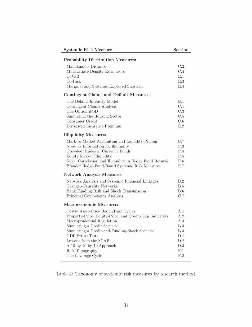
Systemic Risk Measure Section
Probability Distribution Measures:
Mahalanobis Distance C.2Multivariate Density Estimators C.4CoVaR E.1Co-Risk E.3Marginal and Systemic Expected Shortfall E.4
Contingent-Claims and Default Measures:
The Default Intensity Model B.1Contingent Claims Analysis C.1The Option iPoD C.3Simulating the Housing Sector C.5Consumer Credit C.6Distressed Insurance Premium E.2
Illiquidity Measures:
Mark-to-Market Accounting and Liquidity Pricing B.7Noise as Information for Illiquidity F.3Crowded Trades in Currency Funds F.4Equity Market Illiquidity F.5Serial Correlation and Illiquidity in Hedge Fund Returns F.6Broader Hedge-Fund-Based Systemic Risk Measures F.7
Network Analysis Measures:
Network Analysis and Systemic Financial Linkages B.2Granger-Causality Networks B.5Bank Funding Risk and Shock Transmission B.6Principal Components Analysis C.7
Macroeconomic Measures:
Costly Asset-Price Boom/Bust Cycles A.1Property-Price, Equity-Price, and Credit-Gap Indicators A.2Macroprudential Regulation A.3Simulating a Credit Scenario B.3Simulating a Credit-and-Funding-Shock Scenario B.4GDP Stress Tests D.1Lessons from the SCAP D.2A 10-by-10-by-10 Approach D.3Risk Topography F.1The Leverage Cycle F.2
Table 4: Taxonomy of systemic risk measures by research method.
34

3.4.2 Contingent-Claims and Default Measures
With additional structure regarding an institution’s assets and liabilities, it is possible to
construct measures of default likelihood for each institution and then link them either directly
or indirectly through their joint distribution, as in the International Monetary Fund (2009b)
default intensity model. Using a nonparametric estimation technique known as “machine
learning” applied to bank transactions and credit-bureau data for customers of a major U.S.
commercial bank, Khandani, Kim, and Lo (2010) construct nonlinear, non-parametric, out-
of-sample forecasts of consumer credit risk that significantly improve the classification rates
of credit-card delinquencies and defaults.
For a more structural approach to modeling default, Merton (1973) shows that equity
can be viewed as a call option on a firm’s assets, and once a stochastic process for the asset’s
value is chosen, equity and debt contracts on those assets, and implied default probabilities,
can easily be valued using contingent-claims analysis (i.e., derivatives pricing models). This
is the approach taken by Capuano (2008), Gray and Jobst (2010), and Huang, Zhou, and
Zhu (2009a).
Contingent claims analysis can also be applied to measuring the implicit cost of guaran-
tees, as in Khandani, Lo, and Merton’s (2009) simulation of the magnitude of cumulative
losses borne by mortgage lenders through the implicit put option in non-recourse mortgages.
3.4.3 Illiquidity Measures
Illiquidity is an example of a highly specific measure of systemic risk that often requires con-
siderable structure. Because of their role in providing maturity transformation as a valuable
service, banks are vulnerable to funding illiquidity. This fragility forms the rationale for
some of the main weapons in the macroprudential arsenal, including deposit insurance and
the lender of last resort. These issues appear repeatedly in the literature, including recent
papers by Kapadia, Drehmann, Elliott, and Sterne (2009) and Brunnermeier and Pedersen
(2009). The Bank of England has developed its risk assessment model for systemic insti-
tutions (RAMSI) to simulate the possibilities (Aikman, Alessandri, Eklund, Gai, Kapadia,
Martin, Mora, Sterne, and Willison, 2010). Ricks (2010) and Pozsar, Adrian, Ashcraft, and
Boesky (2010) point out that funding troubles can apply to both traditional intermediaries
as well as shadow banks.
Liquidity also affects the other side of the ledger. A key aspect of asset liquidity is
35

the valuation methods used to mark positions, either to model or to market. Sapra (2008)
considers the trade-offs in the choice between these two valuation regimes, and shows benefits
and costs to both. Hu, Pan, and Wang (2010) propose a measure of illiquidity by computing
the deviation of observed market yields on Treasury bonds from their model-based yields
derived from a daily estimate of the zero-coupon curve, and find that deviations are typically
quite low (and liquidity correspondingly high), but spike during crises as arbitrage capital
exits the marketplace. Pojarliev and Levich (2011) use a proprietary high-frequency dataset
of currency funds’ returns to capture the “crowded trade” phenomenon in currency markets.
From a systemic perspective, the most interesting results arise when funding illiquidity and
asset illiquidity interact to generate self-reinforcing feedback of funding shortfalls and asset
fire sales, which propagate to additional funding shortfalls elsewhere. Examples include
Kapadia, Drehmann, Elliott, and Sterne (2009) and Brunnermeier and Pedersen (2009).
Among the approaches described below, Khandani and Lo (2011) propose two distinct
measures of equity market liquidity, one of which is the profitability of an equity mean-
reversion strategy, and the other is a more direct measure of price impact based on Kyle
(1985). For assets that are not publicly traded such as hedge-fund and private-equity re-
turns, Getmansky, Lo, and Makarov (2004) propose using serial correlation as a proxy for
illiquidity. By definition, current prices in illiquid markets are frequently unavailable or unre-
liable, forcing funds to report mark-to-model estimates that often rely on linear extrapolation
pricing methods. Serial correlation in observed returns is an artifact of this autoregressive
smoothing, thus providing an indication of illiquidity.
3.4.4 Network Analysis Measures
Like probability distribution measures, measures of connectedness are largely atheoretical,
but they do offer more direct indications of linkages between firms, and are easily aggre-
gated to produce overall measures of “tight coupling”. One approach is to use principal
components analysis to gauge the degree of commonality among a vector of asset returns.
When the asset returns of a collection of entities are jointly driven by a small number of
highly significant factors, fewer principal components are needed to explain the variation in
the vector of returns, hence sharp increases in the proportion of variability explained by the
first n principal components is a natural indication of systemic risk. The absorption ratio of
Kritzman, Li, Page, and Rigobon (2010) and the PCAS measure of Billio, Getmansky, Lo,
36

and Pelizzon (2010) are based on this property.
More explicit measures of financial networks may be derived from graph theory, a branch
of discrete mathematics in which abstract “nodes” are connected to each other by “edges”
that represent a particular type of relationship. Such networks have been popularized
through social networking websites and degree-of-separation games, but there is a rich set
of analytics that have been developed for networks which can be drawn upon to measure
systemic risk. Chan-Lau, Espinosa, and Sole (2009) and the International Monetary Fund
(2009b) contain two network models of interbank exposures to assess the network external-
ities of a bank failure using institutional data. Using Granger-causality test statistics for
asset returns to define the edges of a network of hedge funds, banks, broker/dealers, and in-
surance companies, Billio, Getmansky, Lo, and Pelizzon (2010) show that Granger-causality
networks are highly dynamic and become densely interconnected prior to systemic shocks.
And the funding gap model of Fender and McGuire (2010a) reveals important linkages
within multinational banks that have many geographically dispersed offices. While aggregate
balance sheet data at the banking-group level may not show much risk, a network map of
the exposures between offices within a banking group may yield a very different picture,
especially for large banking organizations that fund their local foreign currency (especially
USD) positions through their internal (i.e., within the banking group) and external networks.
3.4.5 Macroeconomic Measures
The diametric opposite of the atheoretical probability-distribution measures of Section 3.4.1
are the macroeconomic models of systemic risk. Because the macroeconomy is so complex,
it is virtually impossible to derive useful information from basic macro data without signifi-
cant structural hypotheses. Accordingly, there are a multitude of macroeconomic measures
of systemic risk, corresponding to the many macro models of business and credit cycles,
unemployment, inflation, and growth.
The comprehensive volume by Reinhart and Rogoff (2009) provides useful comparisons
of broad macroeconomic aggregates such as asset price indices (equities, housing, etc.), GDP
growth rates, and public debt over many financial crises, and find a number of common
patterns. Alfaro and Drehmann (2009) use the Reinhart and Rogoff episodes as their starting
point for generating GDP stress tests.
A natural complement to systemic risk measurment is macroprudential regulation, which
37

Borio (2010) defines as calibrating supervision from the top down, rather than building it
up from supervision of individual institutions. Caruana (2010b) makes the case for coun-
tercyclical regulation, arguing that if Basel III had existed at the time of the crisis, banks
would have had much stronger capital bases so that the negative feedback from credit losses
to credit supply—i.e., procyclical aggravation of the business cycle from financial distress—
would have been milder, and the required bailouts much smaller.
Alessi and Detken (2009) construct simple early-warning indicators from a broad range
of real and financial indicators—including GDP and its components, inflation, interest rates,
and monetary aggregates—for 18 OECD countries between 1970 and 2007. Extreme values
of these aggregates are taken as indications of pending booms or busts over the following 6-
quarter horizon. Borio and Drehmann (2009b) propose a related approach, but with signals
defined by simultaneous extreme values for pairs of property prices, equity prices, and credit
spreads, again drawn from 18 industrialized countries between 1970 and 2007.
4 Data Issues
While this survey covers a diverse range of models of threats to financial stability, they all
have one feature in common: significant new data requirements. Although there is still con-
siderable controversy over the root causes of the Financial Crisis of 2007–2009, there is little
dispute that regulators, policymakers, and the financial industry did not have ready access
to information to generate early warning signals or implement rapid resolution plans. For
example, prior to the Dodd Frank Act, even systemically important financial institutions
such as AIG and Lehman Brothers were not obligated to report their amount of financial
leverage, asset illiquidity, counterparty risk exposures, market share, and other critical risk
data to any regulatory agency. If aggregated over the entire financial industry, such data
could have played a crucial role in providing regulators with advance notice of AIG’s unusu-
ally concentrated position in credit default swaps, and the broad exposure of money market
funds to Lehman bonds.
The Dodd Frank Act mandates central reporting of large swaths of the over-the-counter
(OTC) derivatives market, and has assigned to the OFR and FSOC the responsibility for co-
ordinating data collection, data sharing, and supervision of financial firms. Similar efforts are
underway in Europe, with the creation of the European Systemic Risk Board (ESRB). The
Financial Stability Board (FSB) and International Monetary Fund (IMF) are spearheading
38

an effort for the G-20 finance ministers and central bank governors to address information
gaps at the international level (see Financial Stability Board and International Monetary
Fund (2010)). These efforts will undoubtedly raise many new issues surrounding data ac-
quisition, archiving, and management. In this section, we provide a brief introduction to
some of these issues by summarizing in Section 4.1 the data required by the risk analytics
in this survey, reviewing the issues surrounding the standardization of legal entity identi-
fiers (LEIs) in Section 4.2, and discussing recent advances in computer science that have
significant implications for the trade-off between transparency and privacy in Section 4.3.
4.1 Data Requirements
To be able to implement the statistical models and algorithms for calculating various systemic
risk measures described in this paper, risk regulators will have to collect, archive, and access
data on a regular basis, while addressing security and privacy concerns of all stakeholders.
To provide a concrete illustration of the scope of this effort, we provide in Table 5 a detailed
list of the data sources used by the measures in this survey.
4.2 Legal Entity Identifier Standards
Separately, the OFR and FSB are coordinating the development of a standardized legal
entity identifier (LEI) registry, which would, for the first time, provide consistent global
identification of obligors in financial transactions. The LEI has special significance for sys-
temic risk measurement because it facilitates the implementation of many of the network
measures described in this survey.
The need for a standardized method of identification is easiest to see within—but not
limited to—the context of network or graph-theoretic measures such as Chan-Lau, Espinosa,
and Sole (2009) and Duffie (2011), where the nodes in the graph represent legal entities, and
edges represent individual or aggregated contractual relationships. In practical implementa-
tions of such models, especially with systemic scope, both entities and relationships will be
first-class objects with persistent state. This fact implies a need for an efficient, consistent,
globally unique identification scheme for both entities and relationships. An LEI is simply
a systematically maintained tag or code that uniquely identifies an entity in the system.
Bottega and Powell (2010) describe LEIs in detail, noting that they are “a critical compo-
nent in measuring and monitoring systemic risk”, because they enable the construction of
39

Table 5: Data RequirementsReplicable Studies Covered in this Document
Source Asset Type Frequency Start Stop
Asset Price Boom/Bust CycleAlessi and Detken (2009)IMF International Financial Statistics Credit Price Quarterly Q1:1970 Q4:2007OECD Econ Outlook, Main Econ Indicators Macro Macro Annual Q1:1970 Q4:2007OECD Econ Outlook, Main Econ Indicators Macro Macro Quarterly Q1:1970 Q4:2007BIS and ECB sources Money Market Return Quarterly Q1:1970 Q4:2007BIS Real Estate Price Quarterly Q1:1970 Q4:2007
Bank Funding Risk and Shock TransmissionFender and McGuire (2010b)BIS locational banking statistics by nationality Bank Accounting Quarterly Q1:2000 Q1:2010BIS locational statistics by residency Bank Accounting Quarterly Q1:2000 Q1:2010
Consumer CreditKhandani, Kim, and Lo (2010)Proprietary Commercial Bank data Bank Miscellaneous Monthly January 2005 April 2009
Contingent Claims AnalysisGray and Jobst (2010)Moody’s KMV creditEdge Bond Price Quarterly January 1, 2007 January 1, 2010Bloomberg Option Price Daily January 1, 2007 January 1, 2010MarkIt Swap Spread Daily January 1, 2007 January 1, 2010
Co-RiskInternational Monetary Fund (2009a)FRB H15 Release Bond Return Daily July 1, 2003 September 12, 2008CRSP Equity Return Daily July 1, 2003 September 12, 2008Bloomberg Money Market Return Daily July 1, 2003 September 12, 2008FRBNY Website Money Market Return Daily July 1, 2003 September 12, 2008CBOE Website Option Return Daily July 1, 2003 September 12, 2008Bloomberg and Primark Datastream Swap Price Daily July 1, 2003 September 12, 2008
40

Data Requirements (cont.)CoVARAdrian and Brunnermeier (2010)FRBNY Website Bond Return Weekly Q1: 1986 Q1: 2010CRSP Equity Price Weekly Q1: 1986 Q1: 2010COMPUSTAT Equity Accounting Quarterly Q1: 1986 Q1: 2010Bloomberg Money Market Return Weekly Q1: 1986 Q1: 2010FRB H15 Release Money Market Return Weekly Q1: 1986 Q1: 2010CBOE Website Option Return Weekly Q1: 1986 Q1: 2010CRSP Real Estate Return Weekly Q1: 1986 Q1: 2010
Crowded Currency TradesPojarliev and Levich (2011)DB Currency Harvest G10 Index Currency Return Weekly April 2005 June 2010AFX Currency Mgmt. Index Currency Return Weekly April 2005 June 2010DB Currency Volatility Index Currency Return Weekly April 2005 June 2010DB G10 Valuation Index Equity Return Weekly April 2005 June 2010Proprietary Private Partnership Return Weekly April 2005 June 2010
Default IntensityGiesecke and Kim (2009)Moody’s Defaults Risk Services Bond Ratio Static January 1, 1970 December 31, 2008
Distressed Insurance PremiumHuang, Zhou, and Zhu (2009a)Market Participants Bond Probability Weekly January 2001 December 2008Moody’s KMV Bond Probability Weekly January 2001 December 2008FRB H15 Release Bond Spread Weekly January 2001 December 2008TAQ Database Equity Price Tick January 2001 December 2008Bloomberg Equity Return Quarterly January 2001 December 2008FRB H15 Release Money Market Return Weekly January 2001 December 2008Bloomberg Option Implied Vol Weekly January 2001 December 2008MarkIt Swap Spread Daily January 2001 December 2008
Early Warning Macro IndicatorsBorio and Drehmann (2009b)BIS Macro Price Annual 1970 2007BIS Macro Miscellaneous Static 1970 2007
Equity Market LiquidityKhandani and Lo (2011)NYSE Trade and Quote (TAQ) Equity Price Tick July 2, 2007 September 28, 2007
41

Data Requirements (cont.)GDP Stress TestsAlfaro and Drehmann (2009)Authors’ Estimates Macro Miscellaneous Static 1970:Q1 2007:Q4BIS Macro Return Quarterly 1970:Q1 2007:Q4
Granger Causality Networks and PCABillio, Getmansky, Lo, and Pelizzon (2010)CRSP Equity Return Monthly January 1994 December 2008CRSP/Compustat Merged Equity Accounting Quarterly January 1994 December 2008CS/Tremont hedge fund index Private Partnership Return Monthly January 1994 December 2008TASS Database Private Partnership Return Monthly January 1994 December 2008TASS Database Private Partnership Ratio Monthly January 1994 December 2008
Hedge Fund Based Systemic Risk MeasuresChan, Getmansky, Haas, and Lo (2006b, 2006b)TASS Database Private Partnership Return Monthly January 1977 August 2004TASS Database Private Partnership Return Mixed January 1994 August 2004CSFB/Tremont Hedge Fund category indices Private Partnership Return Monthly January 1994 August 2004
Housing SectorKhandani, Lo, and Merton (2009)CRSP Bond Return Monthly February 1977 December 2008Robert Shiller Website Bond Return Annual January 1919 January 1977SandP/Case-Shiller Home Price Composite Real Estate Return Monthly January 1987 December 2008FHFA national house price index Real Estate Return Quarterly Q1: 1975 Q4: 1986Nominal home price index collected by R. Shiller Real Estate Return Annual 1919 1974U.S. Census Bureau Real Estate Number Monthly January 1963 December 2008U.S. Census Bureau Real Estate Number Quarterly 1974 December 2008U.S. Census Bureau Real Estate Price Monthly January 1963 December 2008Freddie Mac Real Estate Return Monthly April 1971 December 2008
Mahalanobis DistanceKritzman and Li (2010)Not Specified by Authors Bond Return Monthly January 1973 December 2009Not Specified by Authors Commodities Return Monthly January 1973 December 2009S&P 500 Equity Return Monthly January 1973 December 2009MSCI non-U.S. Index Equity Return Monthly January 1973 December 2009Not Specified by Authors Real Estate Return Monthly January 1973 December 2009
42

Data Requirements (cont.)Marginal and Systemic Expected ShortfallAcharya, Pedersen, Philippon, and Richardson (2010)CRSP Equity Return Daily June 2006 June 2007CRSP/Compustat Merged Equity Accounting Static June 2007 June 2007MarkIt Swap Spread Daily June 2006 June 2007
Multivariate Density EstimatorSegoviano and Goodhart (2009)MarkIt Swap Spread Daily January 2005 October 2008
Network Analysis of LinkagesInternational Monetary Fund (2009b)BIS Intl. Banking Statistics Mixed Price Static March 2008 March 2008
Noise as Information for IlliquidityHu, Pan, and Wang (2010)CRSP Daily Treasury Database Bond Price, Return Daily January 1987 December 2009
Option iPoDCapuano (2008)Bloomberg Option Price Daily February 12, 2008 June 21, 2008
Principal ComponentsKritzman, Li, Page, and Rigobon (2010)MSCI U.S. Index and 51 Subindices Equity Return Daily January 1, 1998 January 31, 2010For each country, the MSCI Index and all subindices Equity Return Daily January 1, 1998 January 31, 2010Case-Shiller U.S. Housing Price Index Real Estate Return Monthly January 1987 December 2009
Serial Correlation and Illiquidity in Hedge Fund ReturnsGetmansky, Lo, and Makarov (2004)CRSP Equity Price, Return Monthly November 1977 January 2001TASS Database Private Partnership Return Monthly November 1977 January 2001CSFB/Tremont Hedge Fund category indices Private Partnership Price, Return Monthly November 1977 January 2001
10-by-10-by-10Duffie (2011)Bank Executive Survey Mixed Text Quarterly N/A N/A
43

the counterparty network graph of linkages and interrelationships in the system. This is
the foundation of network analysis, as described in Section B, and allows for efficient and
accurate aggregation when searching for concentrated exposures and patterns of activity.
A move toward a globally standardized LEI is already underway, and the OFR is helping
to coordinate an international agreement around a standardized global registry of LEIs.24
A registry of globally unique LEIs has ancillary benefits for the financial industry, which
currently replicates this costly function at each firm to support internal trading, compliance,
and risk management functions.25
The set of instrument types defines the available contractual relationships within the
system—the attributes of the edges between nodes in a counterparty network graph. By
extension, the full set of instrument types establishes the universe of possible portfolios for
market participants. Because there are so many possible contracts, this universe is very
large indeed. The portfolio for a given participant at a particular point in time can be
represented by a vector of numbers, namely the amounts of each contract type contained
in the portfolio. This vector will have many elements, i.e., it will be very high-dimensional.
Moreover, for most participants, it will be very sparsely populated, i.e., it will have zeroes
in most elements, since most participants have relatively specialized activities. Measuring
financial contracts will require the capture of much more detail about those contracts than
is the case under traditional firm-centric accounting systems.
To implement forward-looking risk metrics, the goals should be to capture and understand
each contract’s implied cashflow commitments between the counterparties to the contract,
noting that, in many cases, these cashflows are contingent on other factors. The ability
to work directly with the cashflows is crucial because, in practice, it is possible for two
contracts or portfolios to generate substantially identical cashflow patterns, even when their
24See Office of Financial Research (2011, 2010) for further details.25In November 2010, the Office of Financial Research (2010) issued a policy statement to promote the
development of a global LEI system. This included requirements for attributes of an LEI standard andassociated reference data, as well as operational attributes for a system to issue and maintain LEIs. Simul-taneously, the SEC and CFTC issued “Notices of Proposed Rulemaking” for reporting swap transactions totrade repositories, and expressed a preference for using an LEI for swap reporting. In January 2011, theInternational Organization for Standardization (ISO) launched a process to establish an LEI standard. Itdeveloped a draft specification for the standard and selected a registration authority to oversee assignmentof LEIs: SWIFT, which is partnering with DTCC and its subsidiary Avox as facilities managers. The initialvote on the LEI standard (17442) being developed by ISO closed at the end of June. In September 2011,the Financial Stability Board (FSB) met in Basel to consider options for coordination around governance ofa global LEI infrastructure.
44
legal or accounting representations differ widely. Much of financial engineering is devoted to
repackaging a fixed set of cashflow commitments into a different contractual configuration,
perhaps to manage or lay off risk, avoid taxable events, reduce the market impact of a trade,
or simply to obfuscate the activity.26
4.3 Privacy vs. Transparency
Historically, government policy has tread carefully on the financial industry’s disclosure re-
quirements because much of the industry’s data are considered highly proprietary. Apart
from the obvious privacy issues surrounding customer financial data, the majority of intel-
lectual property in the financial industry consists of trade secrets. Unlike other industries in
which intellectual property is protected by patents, the financial industry consists primarily
of “business processes” that the U.S. Patent Office deems unpatentable, at least until re-
cently.27 Accordingly, trade secrecy is the preferred method by which financial institutions
protect the vast majority of their intellectual property, hence their desire to limit disclosure
of their business processes, methods, and data. Forcing a financial institution to publicly
disclose its proprietary information—and without the quid pro quo of 17-year exclusivity
that a patent affords—will obviously discourage innovation.
Nevertheless, the recent crisis, as well as the skepticism with which the financial industry
has greeted current proposals for systemic-risk surcharges, provide even greater motivation
for the OFR’s mandate to collect data from SIFIs and conduct thorough empirical analysis
on the efficacy of various analytics for capturing systemic risk.
These two seemingly irreconcilable objectives—protecting trade secrets while providing
regulators with systemic risk transparency—are not as difficult to reconcile as they may ap-
pear. In particular, the banking industry already provides a significant amount of proprietary
data to its regulator (the Office of the Comptroller of the Currency) without jeopardizing
its intellectual property, hence some of these procedures may be applied to SIFIs not cur-
rently regulated as banks. However, an even more significant development for systemic
risk management is the recent breakthroughs in cryptography that enable individuals to
26Note that the Dodd Frank Act (see especially section 153(c)(2)) mandates that the FSOC standardizedata types and formats for reporting. Separately, the Committee on Payment and Settlement Systems(CPSS) and International Organization of Securities Commission (IOSCO), at the direction of the FinancialStability Board (FSB), established a task force to define requirements for reporting and aggregation ofover-the-counter (OTC) derivative information.
27See, for example, Lerner (2002).
45
maintain the privacy of their data through encryption algorithms that allow third parties
to compute aggregate statistics across multiple individuals while preserving the privacy of
each individual.28 These algorithms will permit regulators to compute systemic risk expo-
sures without ever requiring individual institutions to reveal their proprietary data; only
encrypted information is used by the regulators. Although still in experimental stages of
development, these so-called “secure multi-party computational” and “fully homomorphic
encryption” algorithms will likely revolutionize the way in which systemic risk is measured
and managed.
5 Conclusions
Regulators have been given a mandate by the Dodd Frank Act to measure and monitor
systemic risk. Market participants have a complementary and immediate interest in better
measurement and management of systemic risk. Although the impact of systemic events is
widely felt, the burden for measuring and monitoring financial stability falls first and foremost
on government regulators, given the unavoidable conflicts of interest faced the private sector.
Because systemic risk is a multifaceted problem in an ever-changing financial environment,
any single definition is likely to fall short, and may create a false sense of security as financial
markets evolve in ways that escape the scrutiny of any one-dimensional perspective.
The scholarly literature is instructive in this regard. A wide variety of measurement
techniques have been proposed and implemented, attempting to capture systemic risk from
diverse perspectives. Ultimately, the specific measures regulators choose to deploy will be-
come the effective operational definition of systemic risk, and these metrics should be chosen
to tackle the problem from many different directions.
The data requirements to support these metrics are correspondingly wide-ranging. In
many cases, academic researchers have made do with publicly available data, adjusting their
modeling approaches accordingly. This is a constraint that regulators will not necessarily
face, given the mandates and authorities granted to them by recent legislation. While the
scholarly literature serves as a useful introduction to the scope of possible measurement
approaches, it should be regarded only as a starting point, not a conclusion. We hope this
survey will expedite the process of discovery and innovation in systemic risk measurement,
28See, for example, Abbe, Khandani, and Lo (2011).
46

and look forward to future editions as more stakeholders engage in this important research
endeavor.
47

Appendix
Note On Attribution: The main goal of this appendix is to present—faithfully—in oneplace and in a consistent format the models and methods developed by other researchers. Tothis end, in the descriptions below we frequently excerpt language from the original publica-tions. While we explicitly cite all excerpted works, we do not typically insert quotation marksor specific footnotes to avoid cluttering the text.
A Macroeconomic Measures
The momentousness of threats to financial stability implies that genuine systemic eventsshould be apparent even at the highest levels of aggregation. The recent book by Reinhartand Rogoff (2009) examines broad macroeconomic aggregates, such as asset price indices(equities, housing, etc.), GDP growth rates, and public debt. They spotlight the irony ofcommon patterns of empirical dynamics of crisis episodes, repeated reliably across countriesand over time. Others exploit the same set of crises; for example, Alfaro and Drehmann(2009) use the Reinhart and Rogoff episodes as their starting point for generating GDP stresstests, described in more detail below. As a matter of regulatory policy, aggregate measuresmay help to identify large-scale imbalances, and suggest strategic policy adjustments toaddress them. Reinhart and Rogoff’s approach also underscores the usefulness of purelyhistorical analyses for guiding regulatory policy.
From a policy perspective, a natural counterpart to macroeconomic risk monitoring ismacroprudential regulation. Borio (2010) defines a macroprudential framework as calibrat-ing supervision from the top down, rather than building it up from supervision of individualinstitutions. This perspective can help resolve a fallacy of composition, if risk is endogenousto the system while nonetheless appearing exogenous to individual firms. It is helpful tothink of both the evolution of risk in a time dimension (e.g., procyclicality) and the alloca-tion of risk in a cross-sectional dimension (e.g., common exposures and interlinkages). PerBorio (2010), the most appropriate risk measures differ for these two dimensions. Earlywarning systems or leading indicators are best for addressing the time dimension, whilesome robust measure of each institution’s contribution to systemic risk is appropriate forthe cross-sectional dimension. Currently, no single measure can do both simultaneously, andin fact, many extant measures can be misleading. He argues that policy implementationshould push rules as far as possible, to counteract the pressures of political economy and thetemptation to discount risks. However, rules should be simple to understand and tolerate adegree of discretion.
Caruana (2010b) argues that if Basel III had existed at the time, banks would havefaced the crisis with much stronger capital bases, so that the negative feedback from creditlosses to credit supply—i.e., procyclical aggravation of the business cycle from financialdistress—would have been milder, and burden on taxpayers smaller. One aspect of BaselIII is a countercyclical capital buffer based on the observation that extraordinary privatecredit growth often ends in widespread defaults.29 In an earlier version, Basel Committee on
29Such a buffer can also serve as a signal for further action. For example, the widening credit and housingprice gaps in the U.S., U.K. and Spain during the 2000s would have pushed a countercyclical buffer against
48

Banking Supervision (2010) emphasized the ratio of credit to GDP as a system-wide bench-mark for accumulating buffers, which would be encouraged through restrictions on capitaldistributions. The virtue of this variable is mainly the fact that it can be computed in nearlyevery country, making cross-country comparisons and coordination easier. However, thereis significant skepticism, especially among central bankers and regulators, around measuresthat may be too esoteric for policymakers charged with making politically unpopular deci-sions. If systemic threats cannot be credibly communicated to political representatives ofthe general population, preemptive action becomes much harder to justify.
More recently, emphasis has shifted instead on an “expected impact” approach basedon a firm’s “systemic footprint,” which proponents argue is more amenable to internationalnegotiation; see Basel Committee on Banking Supervision (2011). At the same time, itis noteworthy that the BIS continues to overload capital requirements with a multitude ofrisk-exposure limits, including market, credit, and operational risk—and now systemic too.Given that both capital and the relevant risks are all measured with error—indeed errorswith potentially procyclical correlation—there is a danger of unintended consequences anda false sense of security arising from this process.
Applying macroeconomic data for early-warning models, Alessi and Detken (2009) con-sider a broad range of real and financial indicators—including GDP and its components,inflation, interest rates, and monetary aggregates—for 18 OECD countries between 1970and 2007. The model emits a yes/no warning when the given indicator exceeds a specificpercentile of its own distribution, forecasting an incipient boom/bust cycle (or lack thereof)over an upcoming 6-quarter horizon. An inaccurate forecast implies either a Type I or TypeII error, and a simple linear mixing variable parameterizes regulators’ choice of preferred (i.e.,least-loss) error. This affects the outcome of “best” indicator, which the authors conclude isthe “global gap”—i.e., the deviation from GDP, after accounting for trends—of either narrowmoney (M1) or private credit.30 Borio and Drehmann (2009b) propose a related approach,but with signals defined by simultaneous extreme values for bivariate pairs of indicators. Thepairings are the three possible combinations of a property price gap, an equity price gap,and a credit gap, again drawn from 18 industrialized countries between 1970 and 2007.31
The authors conclude that best performance occurs for a credit gap exceeding 6%, combinedwith either an equity gap over 60% or a property gap exceeding 15-25%.
A.1 Costly Asset-Price Boom/Bust Cycles
Alessi and Detken (2009) use a signaling methodology to predict costly aggregate asset priceboom/bust cycles. The performance of a host of real and financial variables as early warningindicators for costly aggregate asset price boom/bust cycles are examined, using data for 18
its upper bound for several years. Allowable loan-to-value ratios might have been lowered, or mortgage-interest deductions could have been limited. In the denouement of a boom, the release of the countercyclicalbuffer may further ease financial strains, although the timing of release is not as critical as the timing ofaccumulation, since the latter directly affects the amplitude of the boom and bust.
30Specifically, they define the gap as the detrended ratio of the variable of interest (M1, private credit,etc.) relative to GDP.
31They define “extreme” values as threshold exceedances, and calibrate the model for the most informativethresholds. Specifically, the signaling thresholds for triggering a warning are chosen by a grid search thatoptimizes a signal-to-noise ratio calculated from Type I and Type II errors.
49

OECD countries between 1970 and 2007. A signaling approach is used to predict asset pricebooms that have relatively serious real economy consequences. The authors propose a lossfunction to rank the tested indicators given policymakers’ relative preferences with respectto missed crises and false alarms. The paper analyzes the suitability of various indicators aswell as the relative performance of financial-versus-real, global-versus-domestic, and money-versus-credit-based-liquidity indicators.
A.1.1 Definition
With respect to deciding on what is an acceptable performance for an indicator, the authorsdecide to take into account the regulator’s relative aversion with respect to Type-I and Type-II errors. A warning signal is issued when an indicator exceeds a threshold, here defined bya particular percentile of an indicator’s own distribution. Each quarter of the evaluationsample for each indicator falls into one of the following quadrants of Table A.1 below:
Costly Boom/Bust Cycle No Costly Boom/Bust CycleWithin 6 Quarters Within 6 Quarters
Signal Issued A BNo Signal Issued C D
Table A.1: The “confusion” matrix for the signals.
The loss function used to analyze the usefulness of the indicators is:
L = θC
A+ C+ (1− θ)
B
B +D(A.1)
where θ is the parameter revealing the policymaker’s relative risk aversion between Type-Iand Type-II errors. The usefulness of an indicator can then be defined as:
min[θ; 1− θ]− L . (A.2)
Note that a regulator can always realize a loss of min[θ; 1− θ] by disregarding the indicator.Thus, an indicator is useful to the extent that it produces a loss lower than min[θ; 1− θ] fora given θ.
In order to test their signals, the boom/bust cycles need to be defined. The authorsuse data for 18 OECD countries between 1970:Q1 and 2007:Q4.32 The real aggregate assetprice indexes have been provided by the BIS and are weighted averages of equity prices andresidential and commercial real estate prices, and are deflated by the appropriate nationalconsumption deflators.
An aggregate asset price boom is defined as a period of at least three consecutive quarters,in which the real value of the index exceeds the recursive trend plus 1.75 times the recursivestandard deviation of the series. The recursive trend is calculated with a very slowly adjusting
32The countries are Australia, Belgium, Canada, Switzerland, Germany, Denmark, Spain, Finland, France,the United Kingdom, Ireland, Japan, the Netherlands, Norway, New Zealand, Sweden, the United States.
50

Hodrick-Prescott filter (λ = 100,000) taking into account only data up to the respectivequarter. The authors then differentiate between aggregate asset price booms, which havelittle consequences for the real economy and those that have significant effects. A high-costboom (HCB) is a boom, which is followed by a three year period in which overall real GDPgrowth has been at least three percentage points lower than potential growth. In this way,their sample of 45 classifiable booms is split into 29 high-cost and 16 low-cost booms.
They test a set of 18 real and financial variables and up to 6 different transformationsof these variables, resulting in a total of 89 indicators, on their suitability as early warningindicators for high-cost asset price boom/bust cycles within a 6-quarter forecasting horizon(see Table A.2 for the list of variables).
Variable Category VariableEconomic Variables GDP, consumption, investment, housing investment, CPIFinancial Variables CPI deflated equity, housing prices, the term spread
real exchange rates, real & nominal 3-month interest ratesreal & nominal 10-year bond yields, real M1, real M3real private and domestic credit
GDP (PPP) weighted private credit to GDP, M1/GDP, M3/GDP, nominal short ratesglobal variables VAR shocks for M1, M3, private credit growth
Table A.2: The categories of variables tested as signals.
Note that the real money and credit growth rates have been corrected from endogenousbusiness-cycle and asset-price components by means of recursive vector-autoregression (VAR)models.33 Furthermore, all other variables, except aggregate asset prices, equity prices,exchange rates, and interest rates, are seasonally adjusted.
The evaluation period the authors used was 1979:Q1 to 2002:Q1. They start evaluating in1979 because some starting window is required to compute reasonable initial trend estimates.They do not evaluate the last boom wave because they did not have three years of post-boomGDP data.
There are two main algorithms that the authors apply:
• Individual Country Case: For this case, optimizing the objective function in (A.2)is as follows: for a given θ, for a given indicator, and for a given country, a grid searchis done to find the best percentile in the range [0.05, 0.95] which maximizes (A.2).Note that although this optimal percentile is derived ex post by using all availablehigh-cost booms per country, the threshold varies over time as the percentile is appliedto quarterly updated distributions of the indicator as time passes.
• Individual Indicator Case: For this case, optimizing the objective function in (A.2)is as follows: for a given indicator and a given θ, a grid search is done to find thebest common percentile in the range [0.05, 0.95] across countries; that is, the commonpercentile chosen is the one that minimizes the aggregate loss over all countries.
33Note the subtle but important distinction between the acronym “VAR”, which denotes “vector autore-gression”, and “VaR”, which denotes “value-at-risk”.
51

When computing the resulting figures for A–D of the matrix shown in Table A.1, theauthors exclude boom periods as of the fourth consecutive quarter of which a signal is presentbecause by then, a warning signal is no longer useful.
Apart from the usefulness metric in (A.2), one can also compute the true positives (tp)and the true negatives (tn) for each signal:
tp =A
A +B(A.3)
tn =D
C +D(A.4)
Furthermore, one can compute the difference between the conditional (on a signal beingissued) and unconditional probabilities of the event:
dp =A
A +B− A+ C
A+B + C +D. (A.5)
The larger dp is, the more valuable an indicator it is. Another useful statistic is the averagelead time (ALT) of an indicator, which is defined as the average number of leading quarterswhich an indicator has been signaling an event for the first time.
A.1.2 Inputs and Outputs
• Input: The quarterly time series for the candidate indicators (presented in Table A.2)between 1970:Q1–2007:Q4. All time series except those for asset prices are seasonallyadjusted. Furthermore, the real money and credit growth rates have been correctedfrom endogenous business cycle and asset price components by means of recursive VARmodels.34
Furthermore, a publication lag of 1 quarter is assumed, meaning that an indicator iscalculated for each quarter with variables lagged by 1 quarter.
With respect to the sources of their data, the authors are not too specific as someof it is not public. According to them, the main data source is the OECD EconomicOutlook and Main Economic Indicators. Domestic and private credit are obtained fromthe IMF International Financial Statistics, lines 32 and 32D, respectively. Asset priceindexes were provided by the BIS. Narrow monetary aggregates are from BIS and ECBsources.
• Input: The regulator’s θ. The authors run their analysis for the following: θ =(0.2, 0.3, 0.4, 0.5, 0.6, 0.8).
• Output: The true positives and true negatives (equations (A.3) and (A.4), respec-tively).
34See Adalid and Detken (2007) for a description of the methodology to derive the shocks used to correctthese variables. The VARs are estimated recursively to mimic real-time data availability and 6 quarters ofmoving averages of the derived shocks are used.
52

• Output: The usefulness of each indicator as defined in (A.2).
• Output: The dp as defined in (A.5).
• Output: The average lead time (ALT) of an indicator, defined as the average numberof leading quarters which an indicator has been signaling an event for the first time.
A.1.3 Empirical Findings
The authors find that the global M1 gap and the global private credit gap are the best earlywarning indicators for costly boom/bust cycles. Interestingly, these indicators are globalvariables, which can be explained by the fact that asset price boom/bust cycles are largelyinternational phenomena. However, the “goodness” of an indicator depends on the θ of thepolicymaker; the usefulness of the approach is not breathtaking when policymakers havea clear preference for either Type-I or Type-II errors. In the case of relatively balancedpreferences, the best indicator reduces the preference-weighted sum of Type-I and Type-IIerrors by as much as 25% compared to a situation in which the indicator is ignored.
The best indicator for a policymaker who is only slightly more averse to false alarms thanmissed crises is the global private credit gap. In terms of the absolute performance, usingthe estimated optimal 70% common percentile across countries had a true positive rate of82%. Moreover, the average lead time for the first warning signal was 5.5 quarters.
Overall, the authors find that financial variables contain more information for predictingcostly asset price booms than real indicators, that global financial indicators perform betterthan domestic ones, and that global credit outperforms global money.
The signaling approach as described in their paper is presented in Kaminsky, Lizondo,and Reinhart (1998), and used to predict foreign exchange and banking crises in Borio andLowe (2004) and Borio and Drehmann (2008); these other authors use the signal-to-noiseratio to determine the usefulness of a signal as opposed to the “usefulness” index in equation(A.2).
A.2 Property-Price, Equity-Price, and Credit-Gap Indicators
Borio (2009) construct macroeconomic early warning indicators to predict banking sectorcrises by extending the framework of Borio and Lowe (2004). The three indicators usedare the property price gap, the (real) equity price gap, and the credit gap. This approachis grounded in the endogenous-cycle view of financial instability. The authors argue thatthe coexistence of unusually rapid credit growth and asset prices indicate the build-up offinancial imbalances that raise the likelihood of subsequent financial distress. This approachis similar to that of Alessi and Detken (2009) which is summarized in Section A.1.
A.2.1 Definition
To define the equity-price, property-price, and credit-gap indicators, trends need to be esti-mated. For all three time series, the authors use one-sided Hodrick-Prescott (HP) filters withλ = 1,600, which employ information available only up to the time when the predictions aremade. Using the gaps of the three variables as indicators, the authors try to predict crises
53
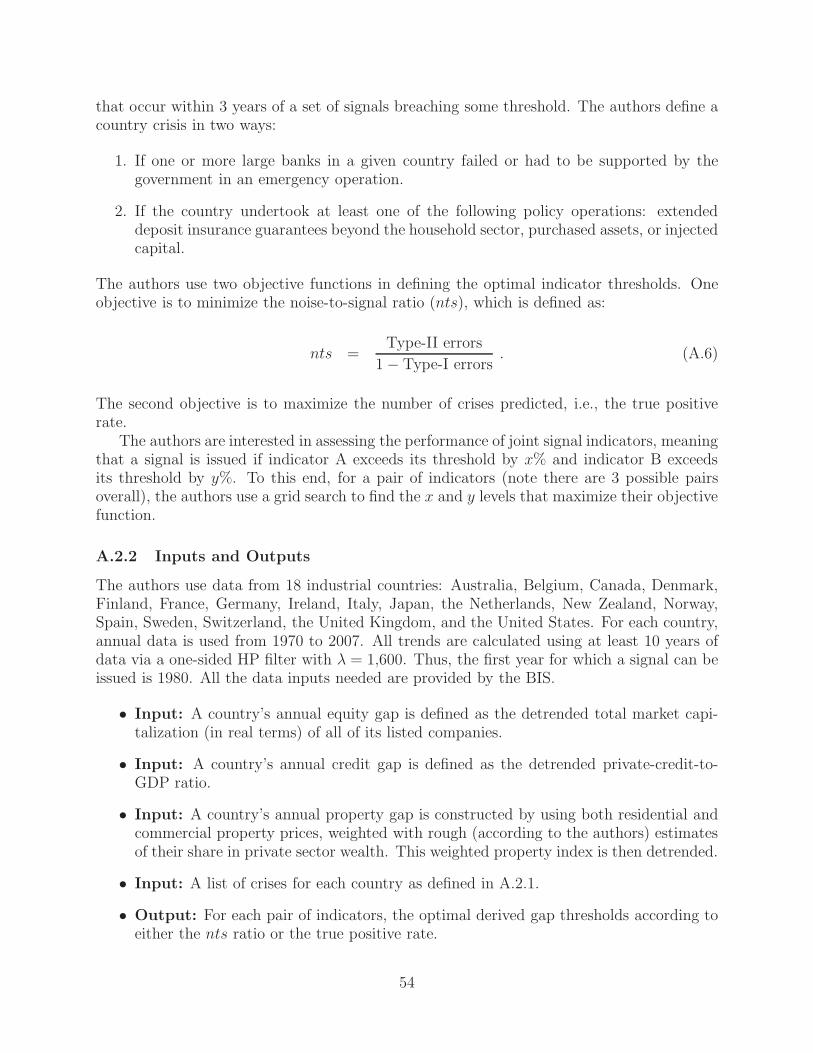
that occur within 3 years of a set of signals breaching some threshold. The authors define acountry crisis in two ways:
1. If one or more large banks in a given country failed or had to be supported by thegovernment in an emergency operation.
2. If the country undertook at least one of the following policy operations: extendeddeposit insurance guarantees beyond the household sector, purchased assets, or injectedcapital.
The authors use two objective functions in defining the optimal indicator thresholds. Oneobjective is to minimize the noise-to-signal ratio (nts), which is defined as:
nts =Type-II errors
1− Type-I errors. (A.6)
The second objective is to maximize the number of crises predicted, i.e., the true positiverate.
The authors are interested in assessing the performance of joint signal indicators, meaningthat a signal is issued if indicator A exceeds its threshold by x% and indicator B exceedsits threshold by y%. To this end, for a pair of indicators (note there are 3 possible pairsoverall), the authors use a grid search to find the x and y levels that maximize their objectivefunction.
A.2.2 Inputs and Outputs
The authors use data from 18 industrial countries: Australia, Belgium, Canada, Denmark,Finland, France, Germany, Ireland, Italy, Japan, the Netherlands, New Zealand, Norway,Spain, Sweden, Switzerland, the United Kingdom, and the United States. For each country,annual data is used from 1970 to 2007. All trends are calculated using at least 10 years ofdata via a one-sided HP filter with λ = 1,600. Thus, the first year for which a signal can beissued is 1980. All the data inputs needed are provided by the BIS.
• Input: A country’s annual equity gap is defined as the detrended total market capi-talization (in real terms) of all of its listed companies.
• Input: A country’s annual credit gap is defined as the detrended private-credit-to-GDP ratio.
• Input: A country’s annual property gap is constructed by using both residential andcommercial property prices, weighted with rough (according to the authors) estimatesof their share in private sector wealth. This weighted property index is then detrended.
• Input: A list of crises for each country as defined in A.2.1.
• Output: For each pair of indicators, the optimal derived gap thresholds according toeither the nts ratio or the true positive rate.
54

A.2.3 Empirical Findings
The authors find that the best performance is achieved if the credit gap exceeds 6% andeither the equity gap exceeds 60% or the property gap exceeds a threshold that rangesfrom 15% to 25%. Especially for horizons of up to 2 years, a property-gap threshold of15% is relatively attractive, as it predicts a high proportion of crises (some 70%), albeit itproduces a higher percentage of false alarms. For a horizon of up to three years, a higherthreshold is preferable, as financial distress does eventually emerge and the nts ratio islower. As expected, the predictive power increases and the nts ratio decreases as the horizonis lengthened, confirming that the timing of the reversal of the financial imbalance is veryhard to predict.
In terms of predicting the recent crisis in the U.S. (this is categorized as a crisis accord-ing to both definitions the authors use), the credit gap was above 6% since 2002, steadilyincreasing to a peak of 12.5% in 2007; furthermore, the property gap was above 15% since2001 and reached a peak of 32% in 2005. Thus, the authors argue that the current crisiswould have been predicted using the methodology described in this section.
A.3 Macroprudential Regulation
According to Borio (2010), a macroprudential framework involves calibrating supervisionfrom a system-wide perspective, rather than from the individual institution basis. It alsomeans taking explicitly into account the fact that drivers of risk depend endogenously on thecollective behavior of financial institutions. The proximate objective of a macroprudentialapproach to regulation is to limit the risk of episodes of system-wide financial distress; itsultimate goal is to contain the costs they generate for the real economy, e.g., output loss.
For analytical convenience, it is helpful to think of the approach as having two dimensions.There is a time dimension, dealing with how aggregate risk in the financial system evolvesover time. There is also a cross-sectional dimension, dealing with how risk is allocatedwithin the financial system at a point in time. To each dimension corresponds a sourceof system-wide financial distress. In the time dimension, the source is the procyclicalityof the financial system; in the cross-sectional dimension, the source is common exposuresand interlinkages in the financial system. To address procyclicality, the principle is to buildcountercyclical buffers. To address common exposures and interlinkages, the principle is tocalibrate prudential tools with respect to the contribution of each institution to systemic risk.This calibration can help ensure that each institution pays for the externality it imposes onthe system.
The time and cross-sectional dimensions also differ on the measures used to assess theircorresponding risks. In the time dimension, the ideal measure would be a fool-proof leadingindicator of financial distress, with a lead sufficient to take remedial action. In the limit, onecould envisage a framework analogous to inflation targeting: instruments would be adjustedso as to maintain the gauge within an acceptable range. In the cross-sectional dimension, theideal measure would allow for a robust quantification of the contribution of each institutionto systemic risk. However, given our state of knowledge, no single measure can performthe two functions simultaneously. In fact, measures that work well in the time dimensionoffer no guidance in the cross-section; and those that work in the cross-section can providethe wrong signals in the time dimension. If one tried to use these market-based measures
55

of systemic risk to address the time dimension, two problems would arise. The measureswould provide the wrong signal: systemic risk would look low when, in fact, it was high.And adjustments for individual institutions’ contributions to systemic risk would actuallyexacerbate procyclicality. This means that market-based measures, unless used as contrarianindicators of risk after suitable normalization, should not be part of leading indicators ofaggregate risk.
With respect to implementing macroprudential regulatory policy, Borio (2010) arguesfor a bold approach in seeking to develop rules as far as possible. Especially in the timedimension, the political economy pressures and the temptation to discount risks can be toopowerful. However, rules should be simple and understandable and a degree of discretionshould be tolerated.
In Caruana’s (2010b) speech on the macroprudential policies of Basel III given in October2010 in China, he argues that if Basel III had existed prior to the crisis, banks would havefaced it with much stronger capital bases, and would have been better able to draw on them.The financial system would have been much better prepared to withstand the shock of fallinghousing prices and losses on securitized assets. As a result, the negative feedback from lossesto credit supply would have been milder, and governments would have had to provide lesssupport. The aggravation of the business cycle (procyclicality) due to the financial systemdistress would have been significantly reduced.
One element of Basel III is the adoption of a countercyclical buffer for banks that issystem-wide in its design. 35 This is based on the fact that private sector credit growth thatis out of line with historical experience often ultimately imposes losses on the lenders. Thusthe ratio of credit to GDP would serve as a common reference for the build-up phase of thebuffer, which would be encouraged through restrictions on capital distributions.
Caruana (2010b) argues that in the U.S., since the early 2000s, the ratio of private creditto GDP and property prices both started going above their trends; a similar phenomenonhappened in the U.K. and Spain during the same period. If the authorities in these threecountries had responded to these observations in a manner consistent with the new counter-cyclical buffer, then the countercyclical capital requirement would have remained at more orless its maximum for some years and the authorities would have been well-advised to considerdoing more. For example, loan-to-value ratios could have been lowered or tax deductions formortgage interest rates on second homes could have been limited. In short, a countercyclicalbuffer at its maximum should be taken as a signal for further action. In all three economies,the countercyclical buffer could have been released some time after mid-2007 in response tofinancial strains and accumulating losses.
However, it should be noted that a late release of the countercyclical buffer would nothave the same unwelcome consequences as a late requirement for it to be accumulated. Ifthe authorities mandate the buffer too late, banks are left vulnerable to losses resulting fromasset price declines; if the authorities release the buffer late, banks can still draw on it, butat the much lower cost of constrained distributions to shareholders.
35Under more recent iterations of Basel III—see Basel Committee on Banking Supervision (2011)—thecountercyclical buffer is overshadowed by the “expected impact” approach.
56
B Granular Foundations and Network Measures
Aggregate measurement of risks and imbalances does not capture everything. For example,aggregation typically tends to average away risk or dispersion in a data set. The financialsector and broader economy are complicated, noisy, and continuously evolving and simpleaggregate metrics cannot transmit enough information to describe the full state of the system.To wit, the extant supervisory framework failed to prevent the 2007–09 crisis, despite anelaborate combination of measurement of aggregates, institution-level capital regulation andon-site examination. The systemic risk measures described in this section exploit a finer-grained instrumentation of the financial system and a more detailed understanding of themodalities of institutional stress and failure. In short, they explore more specifically howsystemic events unfold.36
A discussion of some of the basic building blocks of financial risk measurement is a usefulfoundation for the subsequent discussion of specific approaches. Any measure of financialrisk must involve payment obligations in some way.37 Unless an event or episode provokessome form of default by participants on their promised cashflows, it is unlikely to createa systemic issue. Because of the central role of obligations, legal entities and the financialcontracts between them are basic building blocks for understanding and modeling systemicrisk.38 This appears clearly in a network graph of the financial system, described in moredetail below. By focusing attention on nodes (legal entities) and edges (contracts) the net-work graph emphasizes the role of contractual relationships, as well as a basic distinctionbetween the individual legal entities (the focus of micro-prudential supervision) versus thefinancial system as a whole, which is the subject of macroprudential supervision. In thisconception, each entity (i.e., obligor) is viewed as a “bundle of contracts” with other entitiesin the system, and measuring and modeling contracts becomes a central task for systemicsupervision. Contracts define cashflow obligations, including contingent claims. Contractsare enforceable in court, so there are strong incentives for entities to be diligent in creating anew contract; there is reason to expect that each is reasonably complete and accurate decla-ration of commitments. One should anticipate that data used internally by financial firms foractive business purposes will be more reliable than data created solely for regulatory report-ing. Lastly, contracts serve as an atomistic input for most valuation and risk-managementsoftware packages; as a practical matter contracts are a basic unit of analysis.
Organizing risk measurement around the interacting concepts of contracts and entitiescreates an important requirement for two very basic types of identification data: legal entityidentifiers (LEIs), and instrument types. We discuss this in more detail in Section 4.2, and
36A good example is Duffie (2010).37Many financial contracts (or clauses within a contract) take the form of options or other contingent
claims. Options confer a right, not an obligation, for one of the parties to the transaction. We use the term“obligation” here as shorthand that includes both traditional payment promises as well as option clausesand other contingent claims. If the option-holder exercises its right, the possibility of a payout commitmentbecomes an actual obligation. Similarly, for payouts that depend on an external contingency, these toobecome obligations when the identified contingency occurs.
38It is naive to expect that participants will never make payments unless they are legal obligated. This isnot always the case, even when financial distress looms. For example, in Dec. 2007, Citigroup voluntarilybrought onto its balance sheet $49B in “bankruptcy-remote” assets held in a structured investment vehicle(SIV). As a result of this unilateral move, Citigroup began making payments that had not previously beenlegal obligations of the firm.
57

assume for the remainder of this section that identification has been addressed, though weacknowledge that this is still a work in progress.
One key construct used for modeling granular interlinkages in the financial system isthe counterparty network graph, described, for example, in International Monetary Fund(2009a). A graph is a mathematical formalism—popularized in social networking tools anddegrees-of-separation games—consisting of a set of nodes (legal entities in this case) con-nected by a set of edges (contractual financial relationships). A fully detailed network modelshould make use of the legal entity and instrument type identifiers described above. Someof the natural applications of network tools include measuring the degree of connectivityof particular nodes to determine systemic importance, forecasting or simulating the likelycontagion channels of institutional default or distress, and visualizing an overall “risk map”of exposure concentrations and imbalances in the system. For example, while an individualparticipant concerned about wrong-way risk exposures has only limited visibility into itsguarantor’s other commitments that could be diluting the guarantee, a systemic monitorwith a view of the full counterparty network can see the accumulation of those other ex-posures. While a high-resolution (i.e., granular) examination of the graph at the level ofindividual contracts may be of interest, so too may be the larger imbalances revealed by anaggregation to the level of gross or net exposures between institutions, market sectors, orcountries. Billio, Getmansky, Lo, and Pelizzon (2010) use observable stock market data toimpute estimates of a latent network structure for four classes of institutions: banks, brokers,hedge funds, and insurance companies.39
The data requirements for a fully detailed counterparty network graph are potentiallyextensive. In addition to identifying each legal entity and contractual relationship, detailedattributes for each contract are also desirable because concentrated exposures may be con-tingent on future state and time through specific contractual terms and conditions. Thestatus quo network graph might also be augmented with a conjectural set of possible newexposures, based on institutional rules (e.g., access to the discount window) or historicaltransaction data that expose pre-established counterparty relationships. All this additionaldetail should be helpful in observing concentrated exposures, or in tracing potential channelsof crisis propagation through the system. Simulations of participants’ portfolio adjustmentsas they ramify through the network from a systemic shock, such as the failure of a largedealer, can then reveal the likely systemic significance of such an event, as well as whichentities are most vulnerable. On the other hand, several studies have attempted to infer theunderlying interconnections in the system without directly observing them. For example,the default intensity model described in International Monetary Fund (2009a) focuses on di-rect and indirect systemic linkages among financial institutions. The default intensity modelspecifies a dynamic structure in which defaults occur at random, but tend to be clusteredin time via an event intensity that both builds upon itself and is subject to abrupt ran-dom jumps. The funding gap model of Fender and McGuire (2010b) uses aggregate balancesheet data from the BIS on the banking-group level and the office-location level to infer theconstraints faced by large banking organizations as they attempt to fund their local foreign
39Specifically, they construct a stock market index for each of the four sectors, and extract the four principalcomponents for the returns series. As with the absorption ratio described below, the idea is that systemicrisk will be indicated by a high concentration of the variance on the first principal component. They alsoexamine various network measures of “directional causation” and Granger causality among returns for 100large financial firms (25 chosen from each of their four sectors).
58

currency (especially USD) positions through their internal (i.e., within the banking group)and external networks.
In any financial interlinkage model, it is important to have the correct metric for thevalue of a contract or a portfolio. GAAP accounting provides the most familiar instance,whereby individual contracts are recorded on the general ledger at either historical cost or“fair value.” Under GAAP, fair value is typically implemented as a mark-to-market valua-tion, or a mark-to-model when markets for a particular contractual position are illiquid orinactive.40 Valuation technologies imply some fundamental requirements for risk measure-ment and monitoring, systemic and otherwise. Mark-to-market valuations require up-to-dateprices on comparable securities (or replicating portfolios) traded in active markets. Mark-to-model valuations typically require projections of cashflows for futures dates and contin-gencies, which can be calculated from the detailed terms and conditions of the contract. Inaddition, marks to model require term structures of discount factors for converting thosecashflows to present values. Note that valuation-based metrics are useful both at a systemiclevel as well as at the level of an individual firm; in particular, any measure implicitly orexplicitly involving leverage is intrinsically valuation-based.
An important policy application of models of interconnectedness is the resolution plansnow required for large financial firms. Section 165(d) of the Dodd Frank Act requires non-bank financial companies to report their ownership structure, assets, liabilities, contractualobligations, cross-guarantees, collateral pledges, major counterparties, and significant creditexposures. In essence, each reporting institutions is asked to provide the data to model itsown node and connecting edges for the counterparty network graph. The goal is to facilitatean orderly resolution of the firm in the event of insolvency. In the event of the firm’sinsolvency, this information will make it possible to “cut” the connections that enmesh thefailing firm with the financial network, thus insulating its counterparties from the knock-on effects that might otherwise propagate through the system. Equity-holders would bewiped out, and bondholders would get a “haircut” as conservators stepped in. Over time,an important balance to strike will be giving regulatory authorities sufficient informationto implement their orderly resolution authority without making them responsible for theday-to-day operations of the firm.
The data requirements outlined above for orderly resolution authority are intense, butfeasible (see the discussion in Section 4). In addition to the contractual details that estab-lish the counterparty connections, analysis of the credit exposure report will require creditratings, CDS spreads, and option prices to model the creditworthiness of the identifiedcounterparties. To enable timeliness, this information set should be available—even if notcollected—on a daily basis. To ensure operational capability in the heat of a crisis, a res-olution plan might be subjected to occasional “fire drills” as a matter of course. Indeed,
40Sapra (2008) considers the trade-offs in the choice between these two valuation regimes, concluding thathistorical-cost treatment can lead to inefficient regulatory forbearance if asset values ignore current pricesignals, while mark-to-market treatment can lead to inefficient financial contagion if assets trade in illiquidmarkets with a propensity for significant short-lived price swings (especially in stressful episodes). In eitherregime, such scalar valuations have the important convenience that aggregation across positions is achieved asa simple sum, a fact that carries significant implications for a number of risk monitoring techniques, includingBasel leverage calculations, asset-liability management (ALM), economic value of equity (EVE), etc. In asense, a mark-to-market can be viewed as “crowd-sourcing” across many mark-to-model valuations, since theproviders of market quotes typically arrive at their bids after some sort of modeling, even if unsophisticated.
59
if data formats could be sufficiently standardized to make data ingestion reliably seamless,regulators might even wait and collect the portfolio information from a troubled institutionon an ex post schedule. This should allay some concerns of regulatory micro-management.Regulators have long had resolution authority, but have lacked the operational capability toresolve large, complex institutions in a timely way. The fall-back policy has essentially beenone of “too big/complex to fail”, which has the undesirable side effect of creating a moralhazard. Although a big job, the implementation of living wills has the potential to changethat.
B.1 The Default Intensity Model
Giesecke and Kim (see International Monetary Fund (2009a)) propose a reduced-form statis-tical model for the timing of banking defaults which is designed to capture the effects of di-rect and indirect systemic linkages among financial institutions, as well as regime-dependentbehavior of their default rates. The model is formulated in terms of a default rate, or “in-tensity”, hence the term “default intensity model” (DIM). The default rate jumps at failureevents, reflecting the increased likelihood of further events due to spillover effects. The mag-nitude of the jump is a function of the value of the default rate just before the event. Themodel specification guarantees that the impact of an event increases with the default rateprevailing at the event, a property that is supported by empirical observation. Indeed, theimpact of an event tends to be “regime-dependent”: it is often higher during a default clus-tering episode, when many firms are in a weak condition. However, the impact of an eventdissipates over time.
B.1.1 Definition
Let Tn denote the sequence of economy-wide default times for the universe of Moody’s-ratedcompanies. Let Nt denote the number of defaults that have occurred by time t. Let λt
denote the conditional default intensity, measured in defaults per year, and assume that itevolves through time according to the continuous time equation:
dλt = Kt(ct − λt)dt + dJt (A.7)
where λ0 > 0 is the value of the intensity at the beginning of the sample period, Kt = KλTNt
is the decay rate with which the intensity reverts to the level ct = cλTNtat t, and J is a
response jump process given by:
Jt =∑
n≥1
max(γ, δλT−n)I(Tn ≤ t) (A.8)
where I(Tn ≤ t) = 1 if Tn ≤ t and 0 otherwise. The quantities K > 0, c ∈ (0, 1), δ > 0, andγ > 0 are constant proportional factors, satisfying c(1 + δ) < 1, to be estimated. Equation(A.7) states that the default rate jumps whenever there is a default, reflecting the increasein the likelihood of further events. This specification incorporates the impact of a default onthe surviving firms, which is channeled through direct and indirect systemic linkages. The
60

magnitude of the jump depends on the intensity “just before” the event, which guaranteesthat the impact of an event increases with the default rate prevailing at the time of the event.The parameter γ governs the minimum impact of an event. After the intensity is ramped upat an event, it decays exponentially to the level cλTNt
with rate KλTNt. Since the reversion
rate and level are proportional to the value of the intensity at the previous event, theydepend on the times T1, . . . , Tn and change adaptively at each default. For Tn ≤ t < Tn+1,the behavior of the intensity is described by:
λt = cλTn+ (1− c)λTn
exp (−KλTn(t− Tn)) . (A.9)
The vector parameter to estimate is denoted by θ = (K, c, δ, γ, λ0). The data consist ofobservations of economy-wide default times, Tn during the sample period [0, τ ], which rep-resents daily data from the time period January 1970 to December 2008. The maximumlikelihood problem for the default rate λ = λθ is given by:
maxθ∈Θ
∫ τ
0
(
logλθs−dNs − λθ
s−ds)
(A.10)
where Θ is the set of admissible parameter vectors. The optimization in (A.10) is done viathe Nelder-Mead algorithm, which uses only function values. The algorithm is initializedat a set of random parameter values, which are drawn from a uniform distribution on theparameter space Θ = (0, 2) × (0, 1) × (0, 2)2 × (0, 40). The authors rerun the algorithmfor 100 different initial parameter combinations to check the robustness of the estimates.An alternative brute force way of optimizing (A.10) is to perform a grid search over the 5parameter values on the Θ space defined above.
The authors obtain the following estimates (we have included this as a guide to what
“reasonable” numbers should look like): θ = (0.11, 0.018, 0.13, 0.59, 32.56).Having estimated the model for the economy-wide defaults, one can estimate the distri-
bution of the number of economy-wide defaults during any future time period via a MonteCarlo simulation. Generating the future distribution of defaults is equivalent to generating asequence of inter-arrival times which, in turn, can be generated sequentially by acceptance-rejection sampling from a dominating counting process with intensity λTN
t−≥ λt− . Denote
by τ the current time and H the end of the horizon of interest where H > τ : thus, we seekto generate arrivals in [τ ,H ]. The Monte Carlo steps are:
1. Initialize the time τ parameters (Nτ , TNτ, λTNτ
) according to the model in (A.9).2. Set n = Nτ , S = τ , and λS = cλTn
+ (1− c)λTnexp (−KλTn
(S − Tn)).3. Begin loop.4. Draw ε ∼ exp(λS) and set T = S + ε.5. If T > H then exit loop.6. Else, if T ≤ H : Set λT = cλTn
+ (λS − cλTn) exp (−KλTn
(T − S)).7. Draw u ∼ U(0, 1).8. If u ≤ λT/λS then,9. Set λT = λT +max(γ, δλT ),10. Set T = Tn+1 and update n = n + 1,
61

11. End if.12. Set S = T and λS = λT .13. End loop.
One can run the above simulation multiple times and generate the distribution of economy-wide defaults over the period [τ ,H ]. The last step in estimating the distribution of defaultsin the financial sector is to assign each simulated default to a sector. A sector s ∈ S =
1, 2, . . . , 12 is selected with probability Z(s)∑s∈S Z(s)
, where:
Z(s) =
Nτ∑
n=1
1
1 + τ − Tn
I(Sn = s) (A.11)
where Nτ is the number of defaults observed during the sample period and Sn ∈ S is theobserved sector of the nth defaulter. More weight is assigned to recent observations, i.e.,events that occur closer to the end of the sample period.
Given the estimated distribution of economy-wide events, the systemic risk measure is its95% VaR, i.e., the number of defaults that would occur with a 5% probability, normalizedby the number of firms at the beginning of the period. This measure of systemic risk is nicebecause it is not limited to financial sector defaults. Of course, one can capture the financialsector VaR specifics as well.
B.1.2 Inputs and Outputs
• Input: All corporate defaults from the period January 1, 1970 to December 31, 2008.The data were obtained fromMoody’s Defaults Risk Services. A default event is definedas either (1) a missed or delayed disbursement of interest or principal, including delayedpayments made within a grace period; (2) bankruptcy (as defined by Chapters 7, 10,and 11 of the U.S. commercial code), administration, legal receivership, or other legalblocks to the timely payment of interest or principal; or (3) a distressed exchange thatoccurs when (i) the issuer offers debt-holders a new security or package of securitiesthat amount to a diminished financial obligation; or (ii) the exchange had the apparentpurpose of helping the borrower avoid default.
• Output: The default intensity model parameters θ = (k, c, δ, γ, λ0).
• Output: The distribution of future economy-wide and financial-sector defaults.
• Output: The 95% VaR of the distribution of economy-wide future defaults and the95% VaR of the distribution of financial-system defaults as indicators of systemic risk.
B.1.3 Empirical Findings
The authors find that the DIM quite accurately captures the clustering of the economy-widedefault events, thus suggesting the reliability of the model’s out-of-sample forecasts. Theauthors also generate 1-year predictions of defaults over rolling quarters and find that thetail of the predicted 1-year distribution became quite fat during 2008, exceeding the levels
62
seen during the Internet bubble, suggesting a high probability of further banking failures.In particular, although the number of economy-wide failures for the whole episode of theInternet bubble-bust was substantially higher than the number of defaults observed duringthe recent crisis through the end of 2008, the 1-year predicted distribution of defaults as ofthe end 2008, i.e., the predicted number of defaults for 2009, had a much a fatter tail thanthat for the Internet episode, thus indicating the high likelihood of further defaults in 2009and beyond.
When comparing the 95% VaR for banking sector defaults versus economy-wide defaults,during the 1998–2007 period, the banking sector proved more stable than the economy as awhole. However, during the 2007–2008 period, the authors find sharp parallel increases in theeconomy-wide VaR and the bank-wide VaR, which suggests a break with the past feedbackpatterns, indicating that macro-financial linkages are now tighter, potentially complicatingthe policy response to the financial sector problems.
The DIM was initially used in valuing CDOs and a detailed description can be found inGiesecke and Kim (2009).
B.2 Network Analysis and Systemic Financial Linkages
Chan-Lau, Espinosa, and Sole (2009) and the IMF’s 2009 Global Financial Stability Review(International Monetary Fund, 2009a) contain two network models of interbank exposures toassess the network externalities of a bank failure using institutional data. Network analysis,which can track the reverberation of a credit event or liquidity squeeze throughout thesystem, can provide important measures of financial institutions’ resilience to the dominoeffects triggered by financial distress. The starting point of any network analysis is theconstruction of a matrix of inter-institution exposures that includes gross exposures amongfinancial institutions. Once an exposure matrix is in place, simulations can explore the effectsof the individual default of each bank and then track the domino effects triggered by thisevent. For each bank, one can compute how vulnerable bank A is to bank B’s default andwhich banks cause the most defaults.
Apart from being able to identify systemically important institutions as well as sensitiveinstitutions, this approach can quantify the potential capital losses at various levels, fromthe bank level to the country level. Furthermore, the network approach allows for easyvisualization of the risk map and contagion effects. The main shortcomings of this approachare that detailed inter-institution exposures are required (which is hard to get, especially foroff-balance-sheet items) and that the modeling implicitly assumes static institution behavior.
B.3 Simulating a Credit Scenario
To assess the potential systemic implications of interbank linkages, a network of N institu-tions is considered. The analysis starts with the following stylized balance sheet identity forfinancial institution i :
∑
j
xji + ai = ki + bi + di +∑
j
xij (A.12)
63
where xji stands for bank i loans to bank j, ai stands for bank i ’s other assets, ki stands forbank i ’s capital, bi are long-term and short-term borrowing which are not interbank loans,xij stands for bank i borrowing from bank j, and di are the deposits in bank i.
To analyze the effects of a credit shock, the chapter simulates the individual default ofeach one of the N institutions in the network, and then tracks the domino effects resultingfrom each individual failure. More specifically, for different assumptions of loss given de-fault (denoted by the parameter λ), it is assumed that bank i ’s capital absorbs the losseson impact, and the sequence of subsequent defaults triggered by this event are tracked.For instance, after taking into account the initial credit loss stemming from the default ofinstitution h, the baseline balance sheet identity of bank i becomes:
∑
j
xji − λxhi + ai = (ki − λxhi) + bi + di +∑
j
xij (A.13)
and bank i is said to fail when its capital is insufficient to fully cover its losses, i.e., whenki − λxhi < 0. Subsequent “rounds” of the algorithm take into account the losses stemmingfrom all failed institutions up to that point. Note that λ is typically assumed to be 1 becausewhen the credit event first materializes, banks are unable to recover any of their loans as ittakes time for secondary markets to price recently defaulted instruments. Simulations withλ = 1 should be interpreted as the “on impact” transmission of systemic instability.
B.4 Simulating a Credit-and-Funding-Shock Scenario
To analyze the effects of a credit-and-funding-shock scenario, it is assumed that institutionsare unable to replace all the funding previously granted by the defaulted institutions, which,in turn, triggers a fire sale of assets. Thus, bank i is able to replace only a fraction (1 − ρ)of the lost funding from bank h, and its assets trade at a discount, i.e., their market value isless than their book value, so that bank i is forced to sell assets worth (1 + δ) ρxih in bookvalue terms. Thus, the new balance sheet identity for bank i is given by:
∑
j
xji − (1+δ)ρxih − λxhi + ai = (ki − δρxih − λxhi) + bi + di +∑
j
xij − ρxih . (A.14)
B.4.1 Inputs and Outputs
• Input: The authors use the cross-country bilateral exposures published in the BISInternational Banking Statistics database for March 2008; they restrict themselves tothe “Immediate Borrower Basis” part of the database, which consolidates the data bythe residency of the immediate borrower. From this database, for each country’s bank-ing system, they obtain bilateral exposures for all non-bank asset values, all interbankasset values, all deposit liabilities, all non-bank debt obligations, and all interbank debtobligations. At the individual bank level, these data do not publicly exist althoughclearly, running such simulations at the individual bank level would be more useful.
• Input: Assumptions on the LGD of each bank (λi), the haircut in the fire sale of
64

assets (δ), and the liquidity parameter ρ. These assumptions are at the discretion ofthe regulator; in the paper, λ = 1, δ = 1, and ρ = 0.35.
• Output: The number of induced failures due to an initial bank i failure.
• Output: The hazard rate for bank i, defined as the number of simulations in whichbank i defaults (not including those in which bank i is the initial default bank) over thetotal number of simulations (not including those in which bank i is the initial defaultbank).
• Output: Total capital losses per bank.
B.4.2 Empirical Findings
The authors do not have access to individual bank data so they run the simulations onthe country level by using the BIS International Banking Statistics data for March 2008.When simulating only credit events, they assume a λ of 1; they find that the U.S. and U.K.banking systems are by far the largest systemic risk contributors, as an initial default ofthese banking systems induces the greatest number of failures and the largest capital losses.Interestingly, they find that the most vulnerable banking systems are those of Belgium, theNetherlands, Sweden, and Switzerland as these countries have the highest hazard rates. Forthe case in which both credit and funding events are simulated, the authors find overalllarger capital losses and higher hazard rates. France turns out to be an important liquidityprovider as a French initial failure causes 3 defaults as opposed to 0 in the credit-event-onlycase. Furthermore, the systemic risk posed by a U.S. or U.K. default increases as well, giventhat these two countries’ banking systems also provide liquidity.
The literature on using networks to model financial linkages is vast, and a good surveycan be found in Upper (2007). Another paper which uses networks to study contagion riskin simulated banking systems is Nier, Yang, Yorulmazer, and Alentorn (2008). For sometheoretical underpinnings of the network approach, see the seminal papers by Allen andGale (2000) and Freixas, Parigi, and Rochet (2000). Because central banks typically havethe data needed for such models, there are more references to individual-country bankingsystems, including most of the G10 countries.
B.5 Granger-Causality Networks
Billio, Getmansky, Lo, and Pelizzon (2010) propose two econometric measures of systemicrisk that capture the interconnectedness among the monthly returns of hedge funds, banks,brokers, and insurance companies based on principal components analysis (PCA) and Granger-causality tests. The authors find that all four sectors have become highly interrelated overthe past decade, increasing the level of systemic risk in the finance and insurance industries.Their measures can also identify and quantify financial crisis periods, and seem to containpredictive power for the current financial crisis. Their philosophy is that statistical relation-ships between returns can yield valuable indirect information about the build-up of systemicrisk.
65

B.5.1 Principal Components Analysis
Increased commonality among the asset returns of banks, brokers, insurers, and hedge fundscan be empirically detected by using PCA to decompose the covariance matrix of the four in-dex returns. The returns for hedge funds is proxied by the CS/Tremont hedge fund databaseindex, which is an asset weighted index of fund returns with a minimum of $10 Million inAUM. The return for the “Broker” index is constructed by value weighting the monthlyreturns of all brokers in the CRSP database. The indexes for “Insurers” and “Banks” areconstructed similarly. Given the monthly returns of these 4 indexes, the 4×4 covariancematrix can be estimated as:
Σ ≡ 1
T − 4
T∑
t=1
(Rt − R)(Rt − R)′
(A.15)
where T is the number of months used in the estimation and R denotes the vector of averagereturns. Given the covariance matrix, the 4 eigenvalues can be estimated along with the4 eigenvectors. The authors use the above PCA analysis on 36-month rolling windows ofreturns and track the relative magnitudes of the four eigenvalues as well as the eigenvectorexposures of the two eigenvectors corresponding to the two largest eigenvalues. The ideais that systemic risk is higher when the largest eigenvalue explains most of the variation ofthe data; and the “commonality” between the 4 types of institutions can be seen by thecorresponding entries in the eigenvectors corresponding to the largest eigenvalues: if, forexample, the eigenvector corresponding to the largest eigenvalue has similar entries, then all4 types of institutions have similar exposure to this principal component.
B.5.2 Empirical Findings
The authors find that the first and second principal components capture the majority ofreturn variation during the whole sample. Furthermore, the first principal component is verydynamic capturing from 65% to 93% of return variation; it seems to increase during times ofstress. Interestingly, hedge funds seem to be quite independent of other financial institutions,with significant factor loadings on the third and fourth components, in contrast to the other 3types of institutions which have significant loadings on the first two components. Therefore,hedge funds apparently do not contribute greatly to the covariance matrix of the four indexreturns.
B.5.3 Granger Causality
To investigate the dynamic propagation of systemic risk, the authors also measure the direc-tion of the relationship between institutions using Granger causality: X is said to “Granger-cause” Y if past values of X contain information that helps predict Y above and beyond theinformation contained in past values of Y alone. The mathematical formulation is:
Xt =∑m
j=1 ajXt−j +∑m
j=1 bjYt−j + εt
Yt =∑m
j=1 cjXt−j +∑m
j=1 djYt−j + ηt(A.16)
66

where εt and ηt are two uncorrelated white noise processes and m is the maximum lagconsidered. The definition of causality implies that Y causes X when bj is different fromzero. Likewise X causes Y when cj is different from zero. When both of these statements aretrue, there is a feedback relationship between the time series. The model selection criteria ofthe number of lags considered for the test is based on the Bayesian Information Criterion (seeSchwarz (1978)). The causality is based on the F -test of the null hypothesis that coefficientsbj or cj are equal to zero according to the direction of the Granger causality.
The authors analyze the pairwise Granger causalities between the t and t + 1 monthlyreturns of the 4 indexes; they say that X Granger-causes Y if c1 has a p-value of less than5%; similarly, they say that Y Granger-causes X if the p-value of b1 is less than 5%. Theyadjust for autocorrelation and heteroskedasticity in computing the p-value.
The above Granger-causality analysis can be undertaken at the static level, i.e., over agiven period, find the causal relationships or at the dynamic level, where the analysis is runat 36-month rolling windows and for each window, the dynamic causality index (DCI) iscalculated as:
DCIt =number of causal relationships in window
total possible number of causal relationships(A.17)
Clearly, an increase in the DCI indicates a higher level of system interconnectedness.The authors take a step further and apply the dynamic Granger-causality methodology to
individual institutions. For a given 36-month window, they select the 25 largest institutionsfrom each of the four categories as determined by average market capitalization over theperiod for banks, insurers, and brokers, and by average AUM for hedge funds. They thencompute the “directional” network of these 100 institutions using Granger causalities. Thefollowing set of risk measures can then be computed for each institution:
1. Number of “In” Connections: The number of financial institutions that signifi-cantly Granger-cause this financial institution.
2. Number of “Out” Connections: The number of financial institutions that aresignificantly Granger-caused by this financial institution.
3. Number of “In+Out” Connections: The sum of In and Out connections.
4. Number of “In-from-Other” Connections: The number of other types of financialinstitutions that significantly Granger-cause this financial institution. For example, fora hedge fund, “other types” are banks, brokers, and insurers.
5. Number of “Out-to-Other” Connections: The number of other types of financialinstitutions that are significantly Granger-caused by this financial institution.
6. Number of “In+Out Other” Connections: The sum of “In-from-Other” and“Out-to-Other” connections.
7. Closeness: The shortest path between a financial institution and all other financialinstitutions reachable from it, averaged across all other financial institutions.
67

8. Eigenvector Centrality: For a network with n nodes, let A be the adjacency matrix,the (n×n) matrix of 0’s and 1’s in which the (i, j) element is 1 if there is a connectionbetween nodes i and j, and 0 otherwise. The eigenvector centrality measure is theeigenvector corresponding to the largest eigenvalue of A.
9. PCA: The total absolute exposure of a financial institution to the first 20 principalcomponents weighted by the percentage of the variance explained by each principalcomponent.
An extension of the above Granger-causality approach is to apply a nonlinear version, whichis presented in Billio and Di Sanzo (2006); this nonlinear approach takes into account thecausality relationship based on both the means and volatilities of the financial institutions.
The authors present numerous results based on their Granger causality approach. First,they find that the DCI has been increasing since 1994, with a local peak in 1998, and anotherpeak in 2007–2009; this is consistent with an increase in interconnectedness between insti-tutions which presumably should have a relatively limited overlap in their lines of business.
In terms of evaluating their 9 risk measures presented above in predicting the recentfinancial crisis, the authors rank each institution for each risk measure from 1 to 100. Theyalso compute the maximum percentage loss between July 2007 and December 2008 for eachinstitution. Regressing the rankings of the maximum percentage losses for each institutionon its rankings over the various systemic risk measures, after adjusting for leverage, theyfind that the most important systemic risk measures for an institution are PCA, “Out”,“In+Out”, “Out-to-Other”, “In+Out Other”, “Closeness”, and “Eigenvector Centrality”.
An aggregate systemic risk indicator for a given institution j over a given interval canthus be constructed by estimating the betas of the institution to the 9 risk factors andleverage, and then evaluating the sum:
Ij ≡∑
i∈risk factors
βi (risk factor i ranking of institution j ) . (A.18)
B.5.4 Inputs and Outputs
• Input—Aggregate Index Case: The monthly returns series for the industries ofinterest from January 1994 to December 2008. For hedge funds, this is the returnsof the CS/Tremont hedge fund index. For brokers, the monthly returns and the mar-ket capitalizations of all companies with SIC Codes from 6200 to 6299 in the CRSPdatabase are selected and the value weighted broker index is constructed. The indexesfor banks and insurers are constructed similarly using SIC codes 6000 to 6199 for banksand 6300 to 6499 for insurers.
• Input—Individual Institution Case: The monthly returns series for the largest 25institutions as measured by market capitalization over the 36-month period of interest.The authors run their analyses over rolling 36-month windows from January 1994 toDecember 2008. For brokers, insurers, and banks, the data are obtained from CRSP.For hedge funds, the TASS database is used, which reports individual hedge fundmonthly returns and AUM.
68

• Input—Individual Institution Case: The monthly leverage of the institutions fromJanuary 1994 to December 2008, which is defined as total assets minus equity marketvalue divided by equity market value. For banks, brokers, and insurers, this informationis obtained from the merged CRSP/Compustat database. For hedge funds, they usereported average leverage from the TASS database.
• Output—Both Cases: The time series of the estimated covariance matrices using36-month rolling windows, along with the time series of the corresponding eigenvaluesand eigenvectors.
• Output—Aggregate Index Case: Granger causality relationships between the 4industries for two periods: January 1994 to December 2000 and January 2001 to De-cember 2008.
• Output—Both Cases: The DCI as defined in (A.17).
• Output—Individual Institution Case: The systemic risk indicator for each insti-tution as defined in (A.18).
B.5.5 Related Studies and Further Reading
Chan, Getmansky, Haas, and Lo (2006b, 2006b) found that funding relationships betweenhedge funds and large banks that have brokerage divisions contribute to systemic risk. Theinterconnectedness of brokers and hedge funds has also been considered recently by Kingand Maier (2009), Aragon and Strahan (2009), Brunnermeier and Pedersen (2009), andKlaus and Rzepkowski (2009). Furthermore, Boyson, Stahel, and Stulz (2010) investigatedcontagion from lagged bank and broker returns to hedge fund returns.
B.6 Bank Funding Risk and Shock Transmission
Fender and McGuire (2010a) emphasize the fact that large, international banks tend to haveoffices in many different countries, hence focusing on banking-group-level balance-sheet risksmay ignore important exposures at the individual-office level since these risks are netted outat the group level. Such individual-office frictions may be important, especially during acrisis. A key implication of geographical diversity is that cross-border linkages of individualoffice locations can determine how shocks are transmitted from one location (country) toanother. The authors propose creating undirected and directed networks at the local-officelevel to assess these risks.
The authors also argue that group-level consolidated balance sheets may be misleadingabout funding risk. Only if resources available at one office location can immediately beused elsewhere, i.e., if banks’ internal transfers of funds are perfectly frictionless, will group-level consolidated data provide an adequate picture of any vulnerabilities. As a result, whenviewed from outside the bank using group-level (globally consolidated) data, stresses at theoffice location level can be masked, possibly generating a misleading picture of the overalldegree of funding risk.
For example, at the height of the recent financial crisis, European banks faced problemsborrowing dollars in their home and London offices. These offices typically fund purchases
69

of U.S.-dollar (USD) securities by borrowing USD or swapping domestic currency depositsinto USD. In principle, their local offices, e.g., Korea, could simply send a part of their USDsurplus to cover the needs of the London office (since, typically, local offices are net USDproviders to the market because they borrow USD from their offices at home or elsewhereand swap them into local currency to invest in local assets). Yet, in practice, the extentto which this is possible depends on a variety of factors, including the nature of the localcurrency positions financed with these U.S. dollars, and whether these (and the FX swapsused to obtain local currency) can be unwound in a timely fashion. This unwinding can beparticularly difficult in an environment where many banks are trying to do the same thingor are facing problems or restrictions in the relevant location. Thus, there is a need to beable to assess USD funding gaps not only at the aggregate bank-group level but also at thelocal-office level to develop a more complete understanding of all the possible vulnerabilitiesand their sources.
B.6.1 Definition
The authors use the BIS International Banking Statistics data, from which aggregate consol-idated bank balance sheets can be constructed. However, the data are disaggregated in twoimportant ways. First, for each national banking system (as defined by its headquarters lo-cation), the data provide a picture of the aggregated balance sheet of the underlying entitiesby office location (country level). Second, for each of these banking-system/office-locationpairs, there is a partial breakdown of the location of the counterparties, for both assets andliabilities.
In terms of measuring a banking system’s USD funding gap, the underlying off-balance-sheet FX swap positions must be inferred from reported on-balance sheet activities at thelevel of national banking systems. Specifically, assuming that banks have very small openFX positions, any on-balance-sheet net, i.e., assets minus liabilities, long or short positionin a particular currency provides an estimate of the banks’ offsetting net FX off-balance-sheet swaps positions in that currency. Gauging the funding risk arising from these ac-tivities requires information about the amount of banks’ net short-term USD liabilities atany point in time. This, in turn, necessitates a breakdown by residual maturity of banks’USD-denominated assets and liabilities. Although maturity information is not available,the counterparty type (bank, non-bank or central bank) can serve as a proxy. The stylizedbalance sheet in Table A.3 shows the USD-denominated assets and liabilities of a bankingsystem along with the assumption on their maturity (long-term versus short-term). Specifi-cally, banks’ USD claims on non-banks can be thought of as their desired USD-denominatedinvestment portfolio. In contrast, interbank positions (both assets and liabilities) are typi-cally short term, as are any FX swap positions used to convert funds into USD.
If liabilities to non-banks are all assumed to be long-term, then the lower bound estimateof these banking systems’ overall USD funding gap is:
70
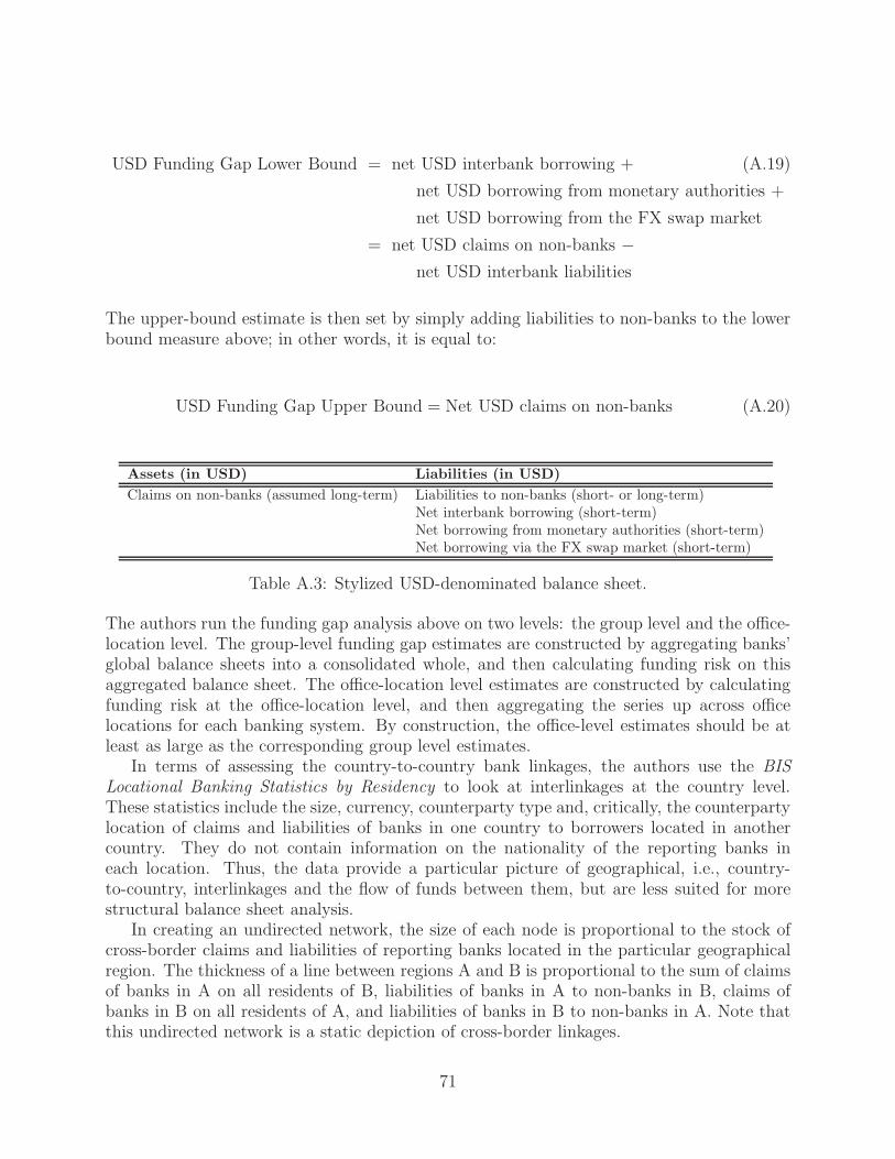
USD Funding Gap Lower Bound = net USD interbank borrowing + (A.19)
net USD borrowing from monetary authorities +
net USD borrowing from the FX swap market
= net USD claims on non-banks −net USD interbank liabilities
The upper-bound estimate is then set by simply adding liabilities to non-banks to the lowerbound measure above; in other words, it is equal to:
USD Funding Gap Upper Bound = Net USD claims on non-banks (A.20)
Assets (in USD) Liabilities (in USD)
Claims on non-banks (assumed long-term) Liabilities to non-banks (short- or long-term)Net interbank borrowing (short-term)Net borrowing from monetary authorities (short-term)Net borrowing via the FX swap market (short-term)
Table A.3: Stylized USD-denominated balance sheet.
The authors run the funding gap analysis above on two levels: the group level and the office-location level. The group-level funding gap estimates are constructed by aggregating banks’global balance sheets into a consolidated whole, and then calculating funding risk on thisaggregated balance sheet. The office-location level estimates are constructed by calculatingfunding risk at the office-location level, and then aggregating the series up across officelocations for each banking system. By construction, the office-level estimates should be atleast as large as the corresponding group level estimates.
In terms of assessing the country-to-country bank linkages, the authors use the BISLocational Banking Statistics by Residency to look at interlinkages at the country level.These statistics include the size, currency, counterparty type and, critically, the counterpartylocation of claims and liabilities of banks in one country to borrowers located in anothercountry. They do not contain information on the nationality of the reporting banks ineach location. Thus, the data provide a particular picture of geographical, i.e., country-to-country, interlinkages and the flow of funds between them, but are less suited for morestructural balance sheet analysis.
In creating an undirected network, the size of each node is proportional to the stock ofcross-border claims and liabilities of reporting banks located in the particular geographicalregion. The thickness of a line between regions A and B is proportional to the sum of claimsof banks in A on all residents of B, liabilities of banks in A to non-banks in B, claims ofbanks in B on all residents of A, and liabilities of banks in B to non-banks in A. Note thatthis undirected network is a static depiction of cross-border linkages.
71
In creating a directed network, times t1 and t2 must be defined. The thickness of an arrowis then proportional to the amount of net bank flows between regions from t1 to t2. Morespecifically, an arrow points from A to B if net flows in this direction are positive, calculatedas changes in net interbank claims (assets minus liabilities) of banks in A on banks in B, plusnet claims of banks in A on non-banks in B, minus net claims of banks in B on non-banksin A.
B.6.2 Inputs and Outputs
In measuring funding risk, ideally one would have data that provide a geographically disag-gregated picture of banks’ consolidated balance sheets. That is, data in which the structureof banks’ global operations (for both assets and liabilities) is visible, and which contain somelevel of information on banks’ operations in various locations, and the interlinkages betweenthese local offices, i.e., inter-office positions, and non-affiliated entities. Currently no datasetexists with this level of detail, nor is such data likely to be available any time soon. Thus,the authors use the BIS International Banking Statistics.
• Input: The group-level balance sheets for each national banking system (as definedby banks’ headquarters location): these are obtained from the BIS Locational Bank-ing Statistics by Nationality database. The authors assess quarterly group-level USDfunding risk estimates over the period from 2000:Q1 to 2010:Q1.
• Input: The balance sheet of the underlying entities by office location (country level)including counterparty locations which are calculated from the BIS Locational Statisticsby Residency data. For the office-location level USD funding risk estimates, the authorsuse quarterly data from 2000:Q1 to 2010:Q1. For the undirected network, the authorsuse the data from 2010:Q1; for the directed network, the authors set t1 = 2000:Q1 andt2 = 2007:Q2.
• Output: USD funding risks at the group-level and at the office-location level.
• Output: Directed and undirected networks of international banking system linkagesat the office-location level.
B.6.3 Empirical Findings
In evaluating the USD funding risks, the authors find that their measures are rough, withvery wide ranges between bounds. However, the indicators do seem to confirm that fundingrisks are actually larger than consolidated data would make them appear. This is a result ofthe netting of interbank and FX swap positions in the group-level estimates. These effectscan be rather large, as suggested by the differences in the lower-bound indicators between thegroup-level and office-level cases for French, Dutch and Belgian banks. Moreover, analysis ofthe underlying office-location-level funding risk measures indicates that a significant portionof the total dollar funding risk is attributable to a given banking system’s foreign offices,about which home country regulators may have only limited information.
In terms of assessing systemic linkages in the international banking system, the authorsfind that capital flows saw a phenomenal reversal in the wake of the recent crisis, in particular
72

out of the United States. Until mid-2007, banks facilitated international capital flows outof Japan and the Eurozone area as well as from Asian financial centers and oil-exportingcountries. Banks routed these funds via offices in the United Kingdom and in Caribbeanfinancial centers, ultimately transferring them to borrowers in the United States and inemerging markets. After the start of the crisis, the direction of many of the bilateral flowsreversed, in part generated by capital movements back to the U.K.
A more detailed exposition of estimating USD funding gaps can be found in Fender andMcGuire (2010b) and Lee (2010).
B.7 Mark-to-Market Accounting and Liquidity Pricing
The most prominent systemic-risk issue associated with mark-to-market accounting is thepotential for fire-sale contagion, as forced sales can depress market prices provoking ad-ditional deleveraging. Laux and Leuz (2010) survey the issues. Adrian and Shin (2010)provide empirical evidence of procyclicality in leverage. They also find that increases in col-lateralized lending in the repo market has significant forecasting power for market volatility.Sapra (2008) considers the trade-offs between historical-cost accounting and mark-to-marketaccounting in the context of a stylized 2-period model in which the banking and insurancesectors interact with liquidity pricing to generate financial contagion.
Proponents of mark-to-market accounting argue that the market price of an asset orliability leads to better insights into the risk profile of firms than a historical-cost-basedmeasurement system. However, moving from a historical-cost regime to a mark-to-marketregime without addressing the other imperfections in the financial system does not guaranteea welfare improvement because mark-to-market accounting creates contagion between thebanking and insurance sectors whereas under historical-cost accounting, there is no conta-gion. The key friction that leads to contagion in the financial system is liquidity pricing; intimes of liquidity shortage, the interaction among institutions and markets can lead to situa-tions where prices no longer reflect fundamentals but rather the amount of liquidity availableto buyers in the market. For both banks and insurers, a large proportion of their balancesheets consists of illiquid claims; these claims are not standardized and do not trade in deepand liquid markets. The historical-cost regime relies on past transaction prices resulting inaccounting values that are insensitive to current price signals. This lack of sensitivity toprice signals induces inefficient sales because the measurement regime does not reflect theappreciated value of the measured assets. Marking to market overcomes this price insensitiv-ity by extracting the information conveyed by current price signals, but in trying to extractinformation about market prices, marking to market potentially adds endogenous volatilityto prices.
The main result of the author’s stylized model is that under historical-cost account-ing, even though fundamentals may be sour, the banks’ solvency requirements rely on pastprices and therefore may incorrectly allow banks to continue operating. By the time regu-lators intervene, it is too late because the size of the banks’ assets is likely to have declinedconsiderably and everyone is worse off. Under mark-to-market accounting, the solvency re-quirements rely on current price signals and are therefore informative about the value of thebanks’ assets, allowing regulators to efficiently shut down the banks earlier, before lossesescalate. However, in the presence of liquidity pricing, contagion is a necessary evil.
The implication of this trade-off is that mark-to-market accounting would dominate
73

historical-cost accounting if the welfare losses from contagion are relatively small comparedto the welfare losses from inefficient continuation under historical-cost accounting. All elsebeing equal, the more illiquid the assets of the bank and therefore the more severe the liq-uidity pricing effect, the more likely it is that historical-cost accounting would dominatemark-to-market accounting from a welfare standpoint.
C Forward-Looking Risk Measurement
A natural extension of valuation-based measures is the broader set of forward-looking riskmeasures. Such metrics can be scalar-valued, like value at risk (VaR) or a CDS spread, ormulti-dimensional, like the coefficients of a multi-factor capital asset pricing model (CAPM).This broader class of risk metrics expands the set in at least three ways. First, when con-trasted with historical-cost valuation, a forward-looking measure should aid in understandingthe evolution of a portfolio, institution, or financial system, even if the metric is not intendedas a forecasting tool. A stark example of the problem is a forward contract, which involvesno up-front payment, but which nonetheless exposes the counterparties to significant risk.Second, unlike valuations, aggregation across positions or portfolios is not necessarily linear,so that simply summing the statistics is typically inappropriate.41 For example, the VaRof a portfolio is not the (weighted) sum of the VaRs of its individual component securities;it depends importantly on correlations and other higher-order attributes of the multivariatereturns distribution. A traditional balance sheet cannot capture such relationships. Third,non-linearity may complicate measurement: unlike simple point estimates, metrics such asconvexity or gamma may explore higher-order contours of a valuation function; similarly,tail dependence statistics and volatility clustering parameters are commonly used to de-scribe higher-order aspects of the returns distribution.
In terms of systemic risk monitoring, assessing forward risk measures may also be usefulin stress testing financial institutions: ideally, some of the stress scenarios should depend onthe forward looking risk metrics.
For purposes of risk measurement—systemic or otherwise—it is important to have aforward-looking view of the cashflows for positions and portfolios at different times in thefuture, and under varying circumstances. As a policy matter, such forward-looking metricsmay help focus regulatory scrutiny on emerging risk factors and other exposures beforethey begin to appear in traditional financial statements. Because the future is not preciselyknowable, risk modeling often postulates one or more probability distributions or stochasticprocesses to capture systematically the patterns that describe the evolution of a portfolio or ofbroader aspects of the financial system. As a familiar example, a short-horizon VaR statisticmight model returns as independent draws from a normal probability distribution, with moresophisticated versions incorporating mean-reversion or volatility clustering. Gray and Jobst(2010) apply Merton (1973)’s model in which equity is viewed as a call option on the assetsof the firm (exercisable by paying the face value of the firm’s debt at maturity), and thevalue of total assets evolves according to a geometric Brownian motion. Among other things,the model generates estimates of the implicit probability of failure/default using observedequity prices as inputs. They apply CDS spreads to back out the proportion of the expected
41This is not always the case. For example, the marginal risk contributions defined in Huang, Zhou, andZhu (2009a) retain the additivity property.
74

loss absorbed by the private sector, with the expected residual loss imposed on the taxpayeras a systemic impact. The financial turbulence model of Kritzman and Li (2010) considersa multivariate case, such as returns on securities in a portfolio. They define “turbulence” asdivergence from typical behavior, and measure it as the Mahalanobis distance of a particularreturns vector from what one should expect based on past observation.42
The measures of Capuano (2008) and Segoviano and Goodhart (2009) both apply maximum-entropy techniques to infer a probability distribution for one or more variables of interest.43
Capuano (2008)’s Option Implied Probability of Default (iPoD) model uses maximum en-tropy to extract market-based default probabilities from prices of equity options. The processexploits the entire information set available from option prices, including volatility smile andskew. One can also obtain the implied expected value of equity, leverage, and the Greeks.44
Segoviano and Goodhart (2009) model systemic risk via the so-called banking system’s mul-tivariate density (BSMD) function, where they define the banking system as a portfolio ofbanks. The maximum-entropy estimation is constrained by the “observed” probabilities ofdistress (PoDs) for the individual institutions, measured via several alternative techniques,including equity options and spreads on credit default swaps. They then use the estimatedBSMD to produce several systemic stability metrics: joint probability of default (JPoD);banking stability index (BSI); distress dependence matrix (DDM); and probability of cas-cade effects (PCE). These measures embed the interdependence structure of distress acrossbanks, capturing not only linear correlation but also nonlinear distress dependencies. More-over, the structure of dependencies changes endogenously as banks’ PoDs change, so thatthe stability measures remain consistent with the economic cycle.
An important class of structural models connects the performance of financial portfolios,such as the cashflow behavior of the underlying financial contracts, to some set of externalfactors. In some cases, such as the underlying for a derivative security, these factors areexplicitly specified, including the rule(s) determining cashflows as a function of the factors. Incontrast, sometimes the particular factors involved and their relationship to the performanceof the portfolio is less explicit. For example, in the housing sector model of Khandani, Lo, andMerton (2009) described above, changes in housing prices have a causal impact on lenders’portfolio losses, even though this empirical relationship is not fixed by a legal commitment.As discussed below, many stress-test approaches have this same flavor.
A scorecard analysis of consumer creditworthiness is another common application of
42Intuitively, the measure assumes a series of concentric, similar (same shape, different sizes) ellipsoidalshells that enclose progressively larger proportions of the scatter plot of historical observations, where theshape of the shells is derived from the covariance matrix of the observations. The Mahalanobis measureis essentially the size of the smallest ellipsoidal shell that just encloses the point (i.e., returns vector) inquestion.
43More specifically, they use the principle of minimum cross-entropy, described in Cover and Thomas(2006). In a nutshell, the maximum entropy method chooses the “best” distribution from among all prob-ability distributions consistent with the known facts about the data-generating process, where “best” isdefined as the distribution with the most entropy (or least explanatory power). In other words, it choosesthe distribution that embeds the fewest extraneous assumptions about the data, beyond what is directlyobservable.
44The “Greeks” is a slang term in mathematical finance for various commonly used model parameters andrisk sensitivity measures for derivatives contracts. The name derives from the fact that these variables aretypically represented by letters of the Greek alphabet (including a made-up letter, “vega”, that does notexist in the Greek language).
75

an external-factors approach. For example, Khandani, Kim, and Lo (2010) apply machine-learning to transactions and credit bureau data from January 2005 to April 2009 for a sampleof customers of a single bank. They construct nonlinear, non-parametric, out-of-sampleforecasts of consumer credit risk that significantly improve the classification rates of credit-card delinquencies and defaults.45 The forecast proportion of delinquencies in the populationfor a given horizon becomes an indicator of systemic risk emanating from consumer lending.
The absorption ratio (AR) of Kritzman, Li, Page, and Rigobon (2010) posits a latentlinear factor structure—essentially, a black box of unnamed external factors—to model thedriving forces underlying the evolution over time of a multidimensional system. The ARis proportion of the variance in the system explained or “absorbed” by a fixed number offactors.46 A higher AR indicates that markets are more tightly coupled, suggesting thatshocks will propagate through the system more quickly. An increased AR is forward-lookinginasmuch as it points to heightened systemic fragility, although by itself this need not leadto volatility or distress. Empirically, they find that the AR for the industry sectors in theMSCI USA index is highly negatively correlated with stock prices and that all of the mostsignificant U.S. stock market drawdowns followed AR spikes within a month. When usingthe 14 subindexes of the Case-Shiller index for housing prices, they find that the AR was aleading indicator of the U.S. housing market bubble.
The data requirements for forward-looking risk metrics and stress testing are extensive.Models that rely on currently and publicly available data—e.g., Capuano (2008), Sego-viano and Goodhart (2009), Adrian and Brunnermeier (2010), International Monetary Fund(2009a), Huang, Zhou, and Zhu (2009b), Kritzman, Li, Page, and Rigobon (2010)—naturallyleverage the forward-looking information value of market prices. This includes equity andoption prices and CDS spreads for financial institutions, but also markets with broader scope,such as stock market price and volatility indexes, exchange rates and housing and commodi-ties prices. Models that posit a latent factor structure—e.g., Khandani, Lo, and Merton(2009), Adrian and Brunnermeier (2010), International Monetary Fund (2009a), Huang,Zhou, and Zhu (2009b), Kritzman, Li, Page, and Rigobon (2010)—tend to focus especiallyon the broader indicators such as interest rates, house-price indexes, aggregate corporatebond spreads, and equity and volatility indexes to summarize the systemic drivers. An ex-ception is Khandani, Kim, and Lo (2010), who had access to confidential portfolio data for asingle institution. Stress testing approaches such as Hirtle, Schuermann, and Stiroh (2009)or Duffie (2011) typically require very specific information about participants’ portfolios, in-cluding contractual terms and conditions and the details of risk-model configurations. Thisallows them to map out in detail the contingent cashflows under various scenarios; becausethe information needs are so intensive, the former occurred only under a regulatory man-date, while the latter remains a proposal. Going forward, the OFR will have the authority
45Specifically, they use generalized classification and regression trees (CARTs) to construct their forecasts.In a CART classifier, the “output” variable (continuous or discrete) is related to a set of independent or“input” variables through a recursive sequence of simple binary relations. CART models are well suitedto problems with high dimensional feature spaces. The forecasted delinquencies are highly correlated withrealized delinquencies. The linear regression R
2 is 85% for both 6- and 12-month horizons, indicating thatthe forecasts are capturing the dynamics of the consumer credit cycle over the sample. However, the rawforecasts consistently underestimate the absolute level of delinquencies by a scalar multiple, a bias that iscorrected by training the estimator on its Type I and Type II errors.
46The latent factors and their loadings are extracted via principal components analysis.
76

to assemble this information. Because detailed portfolio data involve business confidentialinformation, adequate security precautions will be essential.
C.1 Contingent Claims Analysis
Gray and Jobst (2010) propose using contingent claims analysis (CCA) to measure systemicrisk from market-implied expected losses, with immediate practical applications to the anal-ysis of implicit government contingent liabilities, i.e., guarantees. In addition, the frameworkalso helps quantify the individual contributions of financial institutions to overall contingentliabilities in the event of a systemic distress. Based on a sample of the 36 largest financialinstitutions (banks, insurance companies, and asset managers), this systemic risk measure-ment framework generates an estimate of the joint contingent liabilities from market-impliedgovernment support. This approach does not only quantify the magnitude of potential risktransfer to the government but also helps indicate the contribution of individual institutionsto contingent liabilities over time.
C.1.1 Definition
The CCA approach is based on the work pioneered by Merton (1973), which posits that theequity of a firm can be viewed as a call option on its assets and the debt of the firm canbe modeled as being long risk-free debt and short a put option on the firm’s assets. CCAdetermines the risk-adjusted balance sheet of firms, based on the balance sheet identity thatat each instant, a firm’s assets (At) should be equal to the sum of the market value of itsoustanding debt (Dt) and its outstanding equity (Et). Mathematically:
At = Dt + Et . (A.21)
Note that the market value of outstanding debt Dt is different than the face value of out-standing debt B which is due at time T . In order to be able to value the embedded put optionin the firm’s price of debt, the asset value and volatility need to be estimated. Note that theasset value here is not the book value of the assets; it is the “market value” of the assets andis not directly observable. However, the market value of the equity (Et) and its volatility(σE) are observable. Thus, given an asset pricing model, one can back out the current levelof the asset value and its volatility. The authors use the standard Brownian drift-diffusionmodel used in the Black-Scholes-Merton (BSM) option pricing model (see Black and Scholes(1973)):
dAt
At
= rdt + σAdZt (A.22)
where r is the (risk-neutral) drift of At, σA is its volatility, and Zt is a standard geometricBrownian motion. Note that under the risk-neutral measure, the drift is the same as therisk free rate. Given the above asset price model, the price of the equity, which is modeledas a European call option on the assets with a strike price of B, is given by (according to
77

the BSM model):
Et = Atφ(d1) − B exp(−r(T − t))φ(d2) (A.23)
d1 =ln(At/B) + (r + σ2
A/2)(T − t)
σA
√T − t
d2 = d1 − σA
√T − t
where φ(·) denotes the cumulative distribution function (CDF) of the standard normal den-sity function. Furthermore, the following relationship holds:
EtσE = AtσAφ(d1) . (A.24)
Thus, one can solve two equations (A.23) and (A.24) for two unknowns (At and σA). Giventhese parameters, the value of the risky debt can be evaluated: it is equal to the default-freedebt minus the present value of the expected losses due to default, i.e., the price of a putoption on the firm’s assets:
Dt = B exp(−r(t− t)) − PE(t) . (A.25)
The price of the put option can be computed as:
PE(t) = B exp(−r(T − t))φ(−d2)−Atφ(−d1) . (A.26)
The implicit put option calculated for each financial institution from equity market andbalance sheet information using CCA can be combined with information from CDS marketsto estimate the government’s contingent liabilities. If guarantees do not affect equity valuesin a major way, CDS spreads should capture only the expected loss retained by the financialinstitution after accounting for the government’s implicit guarantee. Hence, the scope of themarket-implied government guarantee is defined as the difference between the total expectedloss, i.e., the value of a put option PE(t) derived from the firm’s equity price, and the valueof an implicit put option derived from the firm’s CDS spread. The price of the “CDS putoption” is:
PCDS(t) =(
1− exp (−(sCDS(t)/10000)(B/D(t)− 1)(T − t)))
Be−r(T−t) . (A.27)
Given the CDS put option, we can evaluate the fraction:
α(t) = 1 − PCDS(t)/PE(t) (A.28)
78

of total potential loss due to default covered by implicit guarantees that depress the CDSspread below the level that would otherwise be warranted for the option-implied defaultrisk. In other words, α(t)PE(t) is the fraction of default risk covered by the governmentand (1−α(t))PE(t) is the risk retained by an institution and reflected in the CDS spreads.Thus, the time pattern of the government’s contingent liability and the retained risk in thefinancial sector can be measured.
The measure of systemic risk is given by summing the guarantees over all n institutionsin the sample:
n∑
i=1
αi(t)PiE(t) . (A.29)
The authors also talk about an extension called “systemic CCA” which involves applying theconcept of extreme value theory (EVT) in order to specify a multivariate limiting distributionthat formally captures the potential of extreme realizations of contingent liabilities. However,they do not present the methodology in Gray and Jobst (2010) and the paper they reference(by the same authors) has not yet been published (see Gray and Jobst (2011)).
C.1.2 Inputs and Outputs
The authors ran their analysis for a set of large commercial banks, investment banks, in-surance companies, and special purpose financial institutions between January 1, 2007 andJanuary 31, 2010, but they do not specify which ones.
• Input: Daily at-the-money equity options data from Bloomberg.
• Input: The default horizon T , which is set to 1 year.
• Input: The default barrier B, which is set equal to total short-term debt plus one-halfof long-term debt, consistent with the approach taken by Moody’s KMV CreditEdge.This is re-estimated each quarter for each firm based on its quarterly financial accounts.
• Input: The risk-free rate of interest of 3%.
• Input: Daily 1-year CDS spreads obtained from Markit.
• Output: PE(t) as defined in (A.26).
• Output: The systemic risk indicator as defined in equation (A.29).
C.1.3 Empirical Findings
The authors find a secular increase of implied financial sector support a result of the wideninggap between default risk implied by equity and CDS put option values. Sudden declines inalpha-values around April 2008, October 2008, and May 2009 are attributable to a greateralignment of changes in market capitalization and the market price of default risk, as explicit
79

or implicit financial sector support have little or no impact on slowing the rise of CDS spreadsamid falling equity prices of distressed firms.
Furthermore, the authors find that total expected losses, i.e., the sum of PE(t) over allinstitutions, are highest between the periods just after Lehman’s collapse (September 2008)and end-July 2009; the peak is at 1% of GDP in March 2009. At the peak of the crisis,more than 50% of total expected losses could have been transferred to the government inthe event of default (0.5% of GDP).
C.2 Mahalanobis Distance
Kritzman and Li (2010) define “financial turbulence” as a condition in which asset prices,given their historical patterns of behavior, behave in an uncharacteristic fashion, includingextreme price moves, decoupling of correlated assets, and convergence of uncorrelated assets.They quantify turbulence via the Mahalanobis distance (see Merton (1937)), which measuresthe statistical unusualness of a set of returns given their historical pattern of behavior. Theirmeasure is very general and can be applied across asset classes for which time-series returndata are available.
C.2.1 Definition
Given the returns of n assets, one can define the financial turbulence measure as the squaredMahalanobis distance, as:
dt = (yt −m)′ Σ−1 (yt −m) (A.30)
where:
dt = turbulence at time t
yt = (n×1) vector of asset returns
m = (n×1) sample average vector of asset returns
Σ = (n×n) sample covariance matrix of asset returns
By running this metric over time, one can generate the path of financial turbulence overtime and define as “turbulent” those days for which dt is above its 75th percentile (the restare referred to as “quiet” days).
The application of this systemic risk measure can be used in stress testing portfoliosof assets. In estimating a portfolio’s VaR, the authors suggest using data only from theturbulent periods instead of the full sample. Thus, this turbulence-adjusted VaR betterreflects asset correlations and returns during a turbulent state and is, therefore, a morerealistic estimate of possible losses arising from a systemic event.
80

C.2.2 Inputs and Outputs
• Input: Monthly returns from January 1973 to December 2009 for U.S. Stocks (S&P500), non U.S. Stocks (MSCI non-U.S. index), U.S. Bonds, Real Estate, and Com-modities (they do not specify the data source for the last 3). In general, the frequencyand asset selection can be tailored according to the application.
• Output: The financial turbulence measure in equation (A.30).
• Output: Turbulence-adjusted VaR for a given portfolio.
C.2.3 Empirical Findings
Two empirical features of turbulence are particularly interesting. First, the authors find thatreturns to risk are substantially lower during turbulent periods than during non-turbulentperiods, irrespective of the source of turbulence. Moreover, they find that financial turbulenceis highly persistent. Although the initial onset of financial turbulence cannot be predicted,once it begins, it usually continues for a period of weeks as the markets digest it and reactto the events causing the turbulence.
The authors also test portfolios containing various combinations of U.S. and internationalstocks, U.S. and international bonds, commodities, and real estate. They find that theturbulence-adjusted VaR does a better job of forecasting maximum portfolio losses duringthe financial crisis compared to the standard VaR statistic, which severely underestimatedthe riskiness of these portfolios. To be clear, the turbulence-based approach does not offer amore reliable estimate of when an extreme event will occur; rather, it gives a more reliableestimate of the consequences of such an event.
Other measures of financial distress have been pursued in the literature as well. Correla-tions conditioned on upside or downside market moves are presented in Ang and Chen (2002);time-varying volatility models, such as GARCH models (see for example Bollerslev (1986));Markov regime-switching models (see Ang and Bekaert (2002)); and implied volatility (seeMayhew (1995)) have all been proposed as measures of financial distress.
C.3 The Option iPoD
Capuano (2008) proposes an Option Implied Probability of Default (iPoD) in which market-based default probabilities are inferred from equity options by applying the principle ofminimum cross-entropy (see Cover and Thomas (2006)). The principle of maximum entropyand the related minimum cross-entropy principle make it possible to recover the probabilitydistribution of a random variable. Thus, there is no distributional assumption placed onthe asset nor is there a need to specify any assumption on recovery rates. Furthermore, thedefault barrier is endogenously determined.
The framework exploits the entire information set available from option prices, so as tocapture the well documented volatility smile and skew. One can also obtain the impliedexpected value of equity and leverage as well as the “Greeks”.
81

C.3.1 Definition
The probability of default (PoD) is defined as:
PoD(X) =
∫ X
0
fvdv (A.31)
where fv is the probability density function (PDF) of the value of the asset, and X isthe default threshold. Solving for the PoD uses the cross-entropy functional introduced byKullback and Leibler (see Kullback and Leibler (1951)). The recovered distribution is solelydriven by what the researcher can observe. There is no additional assumption. In this sense,the maximum entropy distribution is the closest to the true distribution, as long as the truedistribution is reflected in the observable data.
The problem to be solved is:
minD
minf(VT )
∫ ∞
VT=0
f(VT ) log
[
f(VT )
f 0(VT )
]
dVT
(A.32)
where f 0(VT ) is the prior probability density function of the value of the asset at time T ,representing the researcher’s prior knowledge on f(VT ), the posterior density. The integrandis the cross-entropy between the prior and the posterior; it represents the degree of uncer-tainty around the posterior. The minimization problem posed in (A.32) is subject to thefollowing 3 constraints:
• Balance Sheet Constraint: The equity can be viewed as a call option on the assets:
E0 = e−rT
∫ ∞
VT=D
(VT −D)f(VT )dVT . (A.33)
• Observable Options Pricing Constraint(s): The resulting density should be ableto price observable option prices:
C i0 = e−rT
∫ ∞
VT = D+Ki
(VT −D −Ki)f(VT )dVT . (A.34)
The above equation states that the present value of the call-option payoff at expirationmust correspond to the observed call-option price today, C i
0 , where i = 1, 2, . . . , nindicates the number of available option contracts. Each option price constraint isweighted by the volume for that option contract over the total volume over all optioncontracts for the same stock and the same expiry; this weight is denoted here by wi.
82

• Normalization Constraint: The PDF must integrate to 1:
1 =
∫ ∞
VT=0
f(VT )dVT . (A.35)
In general, the problem is solved by taking the Frechet derivative of the Lagrangian (see thepaper for details). The end result is:
f(VT , λ) =1
µ(λ)f 0(VT ) × exp
[
λ1e−rT1VT>D(VT −D) +
n∑
i=1
wiλ2,ie−rT1VT>D+Ki
(VT −D −Ki)
]
(A.36)
µ(λ) =
∫ ∞
VT=0
f 0(VT ) × exp
[
λ1e−rT1VT>D(VT −D) +
n∑
i=1
wiλ2,ie−rT1VT>D+Ki
(VT −D −Ki)
]
dVT (A.37)
where 1x>y corresponds to the indicator function that takes the value of 1 whenever x > yand 0 otherwise. To evaluate (A.36), the λs need to be calculated from the constraints. Thisis equivalent to solving the following system:
1
µ(λ)
∂µ(λ)
∂λ1= E0 (A.38)
1
µ(λ)
∂µ(λ)
∂λ2,i= C i
0 for i = 1, 2, . . . , n . (A.39)
This system is highly nonlinear and is solved numerically via Newton minimization. It shouldbe noted that the authors assume a uniform prior distribution.
Overall, when trying to solve for the density, at least 2 option contracts are needed tosolve the problem. One contract is used to pin down D while the other is used to shape thedensity f ∗(VT , D). More contracts are clearly useful to obtain a better representation of thedata.
Suppose that two option contracts are available. The contracts are written on the samestock, and expire on the same date. The empirical strategy consists of using one option con-tract to solve the first optimization problem in (A.32) and using the second option contractto search for the D that is able to price the second option contract. The implementationalgorithm is presented below:
1. Calibrate the maximum value that V can take, Vmax, which is based on the book valueof assets, the average growth rate over the last four quarters of the book value of assets,and its standard deviation.
83

2. Starting from a suitable initial guess of D, call it D0, divide the domain of V into twosub-intervals, DS0 = [0;D0] describing the default state, and NDS0 = [D0 + ε;Vmax]indicating the non-default state.
3. When VT ∈ DS0, discretize the domain by allowing VT to take only two values: 0 orD0 , and start by setting f 0(VT = 0) = 0 and f 0(VT = D0), requiring PoD(D0) = 0.
4. When VT ∈ NDS0, discretize the domain by constructing 100 equally spaced values thatVT can take. Then assign the same likelihood to each of these values (since the prioris a uniform distribution) so that under f 0(VT ), Pr(VT ∈ NDS0) = 1− PoD(D0) = 1.
5. Solve numerically for a new D, called D′, and f(VT , D′) for which f(VT = 0) = 0,
PoD(D′) = f(VT = D′), and Pr(VT ∈ NDS′) = 1− PoD(D′) = 1− f(VT = D′).
Note that for the first iteration, this means the following: given that VT is uniformlydistributed in NDS0, one can solve for D′ by using one option contract to numericallysolve the equation of the form shown in (A.34); given D′, the system of equations(A.36)–(A.39) can be numerically solved for f(VT , D
′).
For subsequent iterations, the new D is found by solving an option contract constraintequation using the density obtained in the previous iteration which is evaluated inthe NDS interval determined at the end of the previous iteration. The significanceof using the new NDS interval is that there (may) be a mass of probability on theleft end. After this new D is obtained, the system of equations (A.36)–(A.39) can benumerically solved for the new density.
6. Once a solution is obtained, repeat steps (3)–(5). However, now fix the range of valuesV can take between DS′ = [0;D′] and NDS′ = [D′+ε;Vmax] , and determine new valuesfor f(VT , D
′′) and D′′.
7. The procedure stops when D′′ = D′ = D∗, so that f ∗(VT , D′) = f ∗(VT , D
′′) =f ∗(VT , D
∗), and Pr(VT ∈ NDS∗) = 1− PoD(D∗) = 1− f ∗(VT = D∗).
8. The option-iPoD corresponds to PoD(D∗).
Note that applying the above algorithm can be used to infer a “term structure” of iPoDs sinceone can use groups of options with different maturities and get an iPoD for each maturity.
C.3.2 Inputs and Outputs
Capuano (2008) estimates the iPoD of 10 U.S. financial institutions: Bank of America, Citi-group, JPMorgan, Wachovia, Wells Fargo, Bear Stearns, Goldman Sachs, Lehman Brothers,Merrill Lynch, and Morgan Stanley. For each bank, the following inputs are needed togenerate its iPoD for a given time interval:
• Input: All European option prices on a given date t for a given maturity T as well astheir volumes and their corresponding strike prices. The author illustrates his methodfor Citigroup, where the date used was February 12, 2008 and the option expiries wereon June 21, 2008. All option data is retrieved from Bloomberg. The volumes areneeded to weight the importance of the option pricing constraints, i.e., wi.
84
• Input: The stock price at the given date t.
• Input: The imposed value of Vmax. The author does not specifically give a formulafor determining Vmax, but from the information given, it seems to be calculated byprojecting the time-t book value of assets to time T by using the average growth rateof the past four quarters plus some multiple of its standard deviation.
• Input: The prior distribution f 0(VT ), which is assumed to be uniform in NDS0 andto be zero in DS0.
• Output: The option-iPoD for the bank.
• Output: The PDF of the asset value at time T , which can be used to estimate othervariables of interest, including the Greeks of the options.
C.3.3 Empirical Findings
First, it should be noted that the framework is not able to describe the PDF in the defaultstate as the inputs are equity option prices, which by definition give no information in thecase of default. However, the framework is informative in determining the probability ofdefault and the PDF of the asset value overall, with the only “adjustments” that the PDFis defined for V ≥ D and that there is a probability mass at V = D which reflects theprobability of default.
In the case of the Bear Stearns collapse, the option-iPoD was able to signal marketsentiment early. Using options expiring on March 22, 2008, the closest to the March 14collapse, the author computes the option-iPoD from February 12 to March 19, 2008 andfinds that the option-iPoD started to indicate some market nervousness on February 21. OnFebruary 29, the option-iPoD jumped by a factor of 766 with respect to the previous day.The following week a relative calm seemed to return, but on March 10 the iPoD jumpedagain, a jump 4 times bigger than the previous one. The iPoD reached its peak on March14, but quickly dropped on March 17, following the rescue plan announced by the FederalReserve. In addition, during this episode, changes in option-iPoD appeared to be a leadingindicator for changes in the level of CDS spreads.
Another paper which uses the minimum cross-entropy approach in deriving probabilitydistributions is Segoviano and Goodhart (2009), which is discussed in Section C.4.
C.4 Multivariate Density Estimators
Segoviano and Goodhart (2009) develop a measure of systemic risk based on the bankingsystem’s multivariate density (BSMD) function. Their approach defines the banking systemas a portfolio of banks and infers its multivariate density from which the proposed measuresare estimated. The proposed BSMDs represent a set of tools to analyze (define) stabil-ity from three different, yet complementary perspectives, by allowing the quantification of“common” distress in the banks of a system, distress between specific banks, and distress inthe system associated with a specific bank, i.e., “cascade effects”. These measures embedthe banks’ distress interdependence structure, which captures not only linear correlation butalso nonlinear distress dependencies among the banks in the system. Moreover, the structure
85
of linear and nonlinear distress dependencies changes endogenously as banks’ probabilitiesof distress (PoDs) change; hence, the proposed stability measures incorporate changes indistress dependence that are consistent with the economic cycle.
C.4.1 Definition
The banking system’s multivariate density characterizes both the individual and joint asset-value movements of the portfolio of banks representing the banking system. It is estimatedvia the minimum cross-entropy method used also in the option-iPoD method (see SectionC.3).
Assume that there are a set of n banks; each bank’s log asset returns is xi. The problemto be solved is:
minp(x1,x2,...,xn)
∫ ∫
· · ·∫
p(x1, x2, . . . , xn) log
[
p(x1, x2, . . . , xn)
q(x1, x2, . . . , xn)
]
dx1dx2 · · · dxn (A.40)
where p(x1, x2, . . . , xn) is the BSMD that we are solving for, q(x1, x2, . . . , xn) is the prior jointprobability density function, and the integrand is the cross-entropy between the prior andthe posterior; it represents the degree of uncertainty around the posterior. The minimizationproblem posed in (A.40) is subject to the following constraints:
• Probability of Default constraints (PoD): For each bank, at time t, the BSMDmust be consistent with the empirically estimated probabilities of default PoDi
t. De-noting bank i’s default barrier as xd
i , its PoD can be written as:
PoDit =
∫ ∫
· · ·∫
p(x1, x2, . . . , xn)1xi<xdidx1dx2 · · · dxn (A.41)
where 1xi<xdiis the indicator function which is nonzero when bank i’s asset value is
below the default barrier xdi . Define as λi the Lagrange multiplier associated with bank
i’s PoD constraint.
• Normalization constraint: The BSMD must integrate to 1:
1 =
∫ ∫
· · ·∫
p(x1, x2, . . . , xn)dx1dx2 · · · dxn . (A.42)
Define as µ the Lagrange multiplier associated with this constraint. The resulting Lagrangian
86
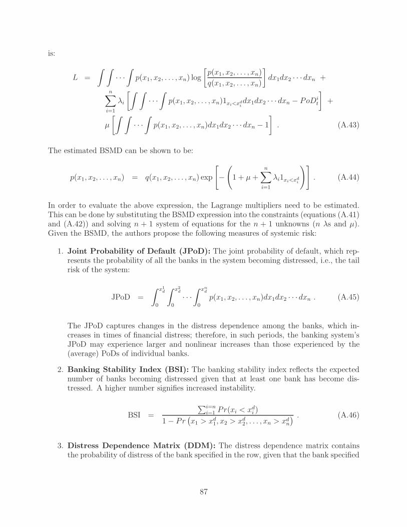
is:
L =
∫ ∫
· · ·∫
p(x1, x2, . . . , xn) log
[
p(x1, x2, . . . , xn)
q(x1, x2, . . . , xn)
]
dx1dx2 · · · dxn +
n∑
i=1
λi
[∫ ∫
· · ·∫
p(x1, x2, . . . , xn)1xi<xdidx1dx2 · · · dxn − PoDi
t
]
+
µ
[∫ ∫
· · ·∫
p(x1, x2, . . . , xn)dx1dx2 · · · dxn − 1
]
. (A.43)
The estimated BSMD can be shown to be:
p(x1, x2, . . . , xn) = q(x1, x2, . . . , xn) exp
[
−(
1 + µ+n∑
i=1
λi1xi<xdi
)]
. (A.44)
In order to evaluate the above expression, the Lagrange multipliers need to be estimated.This can be done by substituting the BSMD expression into the constraints (equations (A.41)and (A.42)) and solving n + 1 system of equations for the n + 1 unknowns (n λs and µ).Given the BSMD, the authors propose the following measures of systemic risk:
1. Joint Probability of Default (JPoD): The joint probability of default, which rep-resents the probability of all the banks in the system becoming distressed, i.e., the tailrisk of the system:
JPoD =
∫ x1d
0
∫ x2d
0
· · ·∫ xn
d
0
p(x1, x2, . . . , xn)dx1dx2 · · · dxn . (A.45)
The JPoD captures changes in the distress dependence among the banks, which in-creases in times of financial distress; therefore, in such periods, the banking system’sJPoD may experience larger and nonlinear increases than those experienced by the(average) PoDs of individual banks.
2. Banking Stability Index (BSI): The banking stability index reflects the expectednumber of banks becoming distressed given that at least one bank has become dis-tressed. A higher number signifies increased instability.
BSI =
∑i=ni=1 Pr(xi < xd
i )
1− Pr(
x1 > xd1, x2 > xd
2, . . . , xn > xdn
) . (A.46)
3. Distress Dependence Matrix (DDM): The distress dependence matrix containsthe probability of distress of the bank specified in the row, given that the bank specified
87
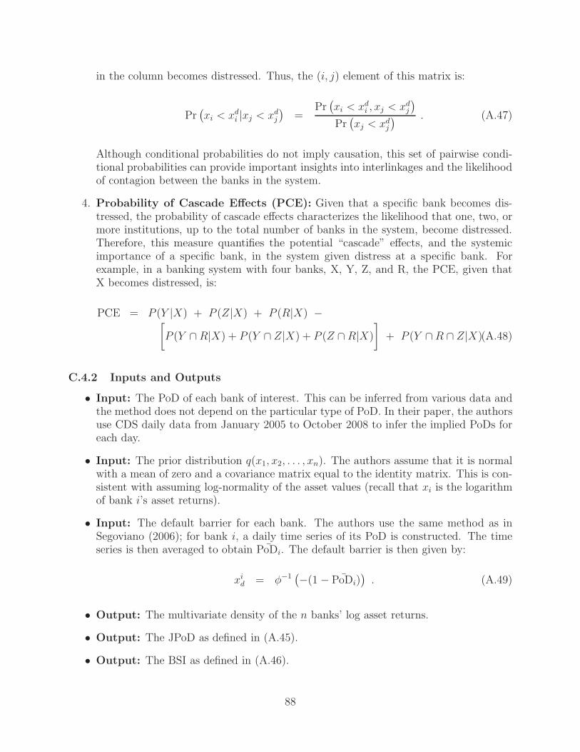
in the column becomes distressed. Thus, the (i, j) element of this matrix is:
Pr(
xi < xdi |xj < xd
j
)
=Pr(
xi < xdi , xj < xd
j
)
Pr(
xj < xdj
) . (A.47)
Although conditional probabilities do not imply causation, this set of pairwise condi-tional probabilities can provide important insights into interlinkages and the likelihoodof contagion between the banks in the system.
4. Probability of Cascade Effects (PCE): Given that a specific bank becomes dis-tressed, the probability of cascade effects characterizes the likelihood that one, two, ormore institutions, up to the total number of banks in the system, become distressed.Therefore, this measure quantifies the potential “cascade” effects, and the systemicimportance of a specific bank, in the system given distress at a specific bank. Forexample, in a banking system with four banks, X, Y, Z, and R, the PCE, given thatX becomes distressed, is:
PCE = P (Y |X) + P (Z|X) + P (R|X) −[
P (Y ∩R|X) + P (Y ∩ Z|X) + P (Z ∩ R|X)
]
+ P (Y ∩R ∩ Z|X) .(A.48)
C.4.2 Inputs and Outputs
• Input: The PoD of each bank of interest. This can be inferred from various data andthe method does not depend on the particular type of PoD. In their paper, the authorsuse CDS daily data from January 2005 to October 2008 to infer the implied PoDs foreach day.
• Input: The prior distribution q(x1, x2, . . . , xn). The authors assume that it is normalwith a mean of zero and a covariance matrix equal to the identity matrix. This is con-sistent with assuming log-normality of the asset values (recall that xi is the logarithmof bank i’s asset returns).
• Input: The default barrier for each bank. The authors use the same method as inSegoviano (2006); for bank i, a daily time series of its PoD is constructed. The timeseries is then averaged to obtain ¯PoDi. The default barrier is then given by:
xid = φ−1
(
−(1 − ¯PoDi))
. (A.49)
• Output: The multivariate density of the n banks’ log asset returns.
• Output: The JPoD as defined in (A.45).
• Output: The BSI as defined in (A.46).
88
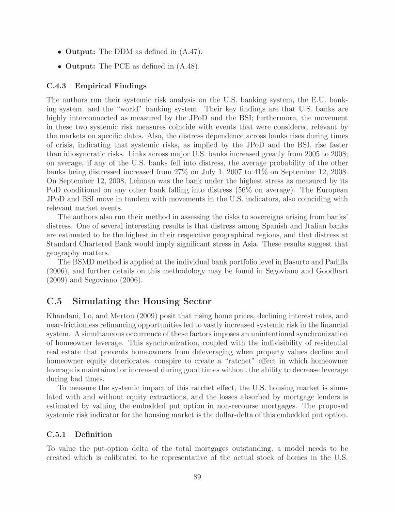
• Output: The DDM as defined in (A.47).
• Output: The PCE as defined in (A.48).
C.4.3 Empirical Findings
The authors run their systemic risk analysis on the U.S. banking system, the E.U. bank-ing system, and the “world” banking system. Their key findings are that U.S. banks arehighly interconnected as measured by the JPoD and the BSI; furthermore, the movementin these two systemic risk measures coincide with events that were considered relevant bythe markets on specific dates. Also, the distress dependence across banks rises during timesof crisis, indicating that systemic risks, as implied by the JPoD and the BSI, rise fasterthan idiosyncratic risks. Links across major U.S. banks increased greatly from 2005 to 2008;on average, if any of the U.S. banks fell into distress, the average probability of the otherbanks being distressed increased from 27% on July 1, 2007 to 41% on September 12, 2008.On September 12, 2008, Lehman was the bank under the highest stress as measured by itsPoD conditional on any other bank falling into distress (56% on average). The EuropeanJPoD and BSI move in tandem with movements in the U.S. indicators, also coinciding withrelevant market events.
The authors also run their method in assessing the risks to sovereigns arising from banks’distress. One of several interesting results is that distress among Spanish and Italian banksare estimated to be the highest in their respective geographical regions, and that distress atStandard Chartered Bank would imply significant stress in Asia. These results suggest thatgeography matters.
The BSMD method is applied at the individual bank portfolio level in Basurto and Padilla(2006), and further details on this methodology may be found in Segoviano and Goodhart(2009) and Segoviano (2006).
C.5 Simulating the Housing Sector
Khandani, Lo, and Merton (2009) posit that rising home prices, declining interest rates, andnear-frictionless refinancing opportunities led to vastly increased systemic risk in the financialsystem. A simultaneous occurrence of these factors imposes an unintentional synchronizationof homeowner leverage. This synchronization, coupled with the indivisibility of residentialreal estate that prevents homeowners from deleveraging when property values decline andhomeowner equity deteriorates, conspire to create a “ratchet” effect in which homeownerleverage is maintained or increased during good times without the ability to decrease leverageduring bad times.
To measure the systemic impact of this ratchet effect, the U.S. housing market is simu-lated with and without equity extractions, and the losses absorbed by mortgage lenders isestimated by valuing the embedded put option in non-recourse mortgages. The proposedsystemic risk indicator for the housing market is the dollar-delta of this embedded put option.
C.5.1 Definition
To value the put-option delta of the total mortgages outstanding, a model needs to becreated which is calibrated to be representative of the actual stock of homes in the U.S.
89

In the simulation, each house enters when it is first sold, and stays until its mortgage isfully paid. In the process, the house may be refinanced one or more times. The decisionrule on whether to refinance is a function of the loan-to-value ratio and is calibrated so as toreproduce historical housing data such as the total value of residential mortgages outstandingand the total value of equity extracted from homes. The simulation that the authors runuses the following assumptions:
1. Each house is purchased at an initial LTV0 of 85%.
2. All homes are purchased with conventional 30-year fixed-rate mortgages that are non-recourse loans.
3. The market value of all houses that are in “circulation”, i.e., that have outstandingmortgages and may be refinanced at some point, grows at the rate given by the HomePrice Index (HPI).
4. Only national data on home sales, price appreciation, and mortgages outstanding areused to calibrate the simulation.
5. A homeowner’s decision to refinance is made each month, and is only a function ofthe current equity in the home and the potential savings from switching to a lowerinterest-rate mortgage.
6. For rate refinancing, also called “no-cash-out” refinancing, the owner will refinancewhen rates have fallen by more than 200 basis points. The new mortgage is assumedto have the same maturity as the existing mortgage, and the principal of the newmortgage is equal to the remaining value of the existing mortgage. Therefore, there isno equity extracted from the house in this case.
7. For cash-out refinancings, the homeowner will refinance to take out the maximumamount of equity possible. Therefore, the LTV ratio will be brought back to LTV0
after each refinancing, and a new loan with a maturity of 30 years will be originated.
8. The refinancing decisions by homeowners are random and independent of each other,apart from the dependence explicitly parameterized in the refinancing rule.
9. Once fully owned, a home will not re-enter the market.
The total value of all homes at time t is the total value of all homes that were either directlypurchased at time t or were purchased in an earlier period, survived until time t − 1, andcash-out refinanced at time t.
TOTALVt = NHt ×VALUEt,t +
t−1∑
i=1
TOTALVi × SURVIVi,t−1 × REFIi,t ×VALUEi,t
VALUEi,i
(A.50)where NHt is the number of new homes entering the system in vintage t, SURVIVi,t−1 isthe probability that a new home from vintage i has not undergone a cash-out refinancingby time t − 1, and REFIi,t is the probability that a home entering the system in vintage i
90

undergoes a cash-out refinancing at date t, conditioned on the event that it has not yet beenrefinanced by date t. The variable VALUEi,t is the value of a house from vintage i by timet, where i ≤ t. Thus, VALUEi,i = NHPi, where NHPi is the average price for all new homessold in vintage i. The value for all subsequent periods grows at the rate given by the HPI.Thus, the multiplier VALUEi,t/VALUEi,i is an adjustment factor that reflects time variationin housing prices.
The authors find that the following decision rule calibrates the simulation well to thehistory of outstanding mortgage volume and to historical equity extractions:
REFIi,t =
0% if LTVi,t = 0
0.3% if t ≤ 1988 and LTVi,t ∈ (0%, 85%]
0.9% if t ≥ 1989 and LTVi,t ∈ (0%, 85%]
. (A.51)
Thus, before 1989, the probability of refinancing is 0.3% for homes with LTV less than 85%.After 1989, there is a structural break and the probability of refinancing is higher at 0.9%for homes with LTV less than 85%. Given this decision rule, the variables SURVIVi,t−1
and REFIi,t are determined and thus TOTALVt in (A.50) can be evaluated. The abovesimulation is called the “cash-out” refinancing simulation.
To understand the effects of the cash-out refinancing simulation above, the authors alsorun a simulation where only rate refinancing occurs as described in Assumption 6 above;this is called the “no-cash-out” refinancing simulation. It is equivalent to evaluating (A.50)where REFi,t = 0 and SURVIVi,t = 1 for all i and t. Clearly, this is not realistic but it isthe baseline scenario of risk due to the fact that the dynamics of LTVs are driven purely byhome price changes as opposed to the cash-out refinancing case, where equity extractionsplay an important role in the dynamics of LTVs.
To evaluate the value of the embedded put option on the total value of homes outstanding,a stochastic process for housing prices needs to be specified. The authors assume that housingprices follow a discrete-time geometric random walk represented by a recombining tree andthat markets are dynamically complete so that options on property values can be pricedby no-arbitrage arguments alone. The put option is assumed to be “Bermudan”, meaningthat it can be exercised on a set of fixed dates: these exercise dates are once a month,just prior to each mortgage payment date. The exercise price is the amount of principaloutstanding on the loan, which declines each month due to the monthly mortgage payments.Furthermore, a volatility of 8% and a rental “yield” of 4% are assumed. For a detailedexplanation of binomial tree option pricing methods, see Cox and Rubinstein (1985); a moregeneral discussion of option pricing can be found in Hull (2000).
Denote by GRTi,t the value of the guarantee, i.e., the put option, calculated for a singlehome from vintage i at time t. Then, the aggregate value of the guarantees is:
TOTALGRTt =
t∑
i=1
TOTALVi × SURVIVi,t ×GRTi,t
VALUEi,i
. (A.52)
91
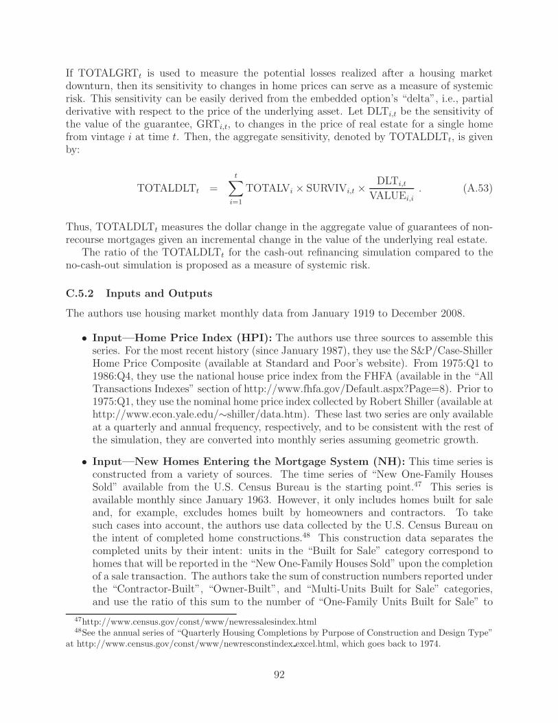
If TOTALGRTt is used to measure the potential losses realized after a housing marketdownturn, then its sensitivity to changes in home prices can serve as a measure of systemicrisk. This sensitivity can be easily derived from the embedded option’s “delta”, i.e., partialderivative with respect to the price of the underlying asset. Let DLTi,t be the sensitivity ofthe value of the guarantee, GRTi,t, to changes in the price of real estate for a single homefrom vintage i at time t. Then, the aggregate sensitivity, denoted by TOTALDLTt, is givenby:
TOTALDLTt =
t∑
i=1
TOTALVi × SURVIVi,t ×DLTi,t
VALUEi,i
. (A.53)
Thus, TOTALDLTt measures the dollar change in the aggregate value of guarantees of non-recourse mortgages given an incremental change in the value of the underlying real estate.
The ratio of the TOTALDLTt for the cash-out refinancing simulation compared to theno-cash-out simulation is proposed as a measure of systemic risk.
C.5.2 Inputs and Outputs
The authors use housing market monthly data from January 1919 to December 2008.
• Input—Home Price Index (HPI): The authors use three sources to assemble thisseries. For the most recent history (since January 1987), they use the S&P/Case-ShillerHome Price Composite (available at Standard and Poor’s website). From 1975:Q1 to1986:Q4, they use the national house price index from the FHFA (available in the “AllTransactions Indexes” section of http://www.fhfa.gov/Default.aspx?Page=8). Prior to1975:Q1, they use the nominal home price index collected by Robert Shiller (available athttp://www.econ.yale.edu/∼shiller/data.htm). These last two series are only availableat a quarterly and annual frequency, respectively, and to be consistent with the rest ofthe simulation, they are converted into monthly series assuming geometric growth.
• Input—New Homes Entering the Mortgage System (NH): This time series isconstructed from a variety of sources. The time series of “New One-Family HousesSold” available from the U.S. Census Bureau is the starting point.47 This series isavailable monthly since January 1963. However, it only includes homes built for saleand, for example, excludes homes built by homeowners and contractors. To takesuch cases into account, the authors use data collected by the U.S. Census Bureau onthe intent of completed home constructions.48 This construction data separates thecompleted units by their intent: units in the “Built for Sale” category correspond tohomes that will be reported in the “New One-Family Houses Sold” upon the completionof a sale transaction. The authors take the sum of construction numbers reported underthe “Contractor-Built”, “Owner-Built”, and “Multi-Units Built for Sale” categories,and use the ratio of this sum to the number of “One-Family Units Built for Sale” to
47http://www.census.gov/const/www/newressalesindex.html48See the annual series of “Quarterly Housing Completions by Purpose of Construction and Design Type”
at http://www.census.gov/const/www/newresconstindex excel.html, which goes back to 1974.
92

adjust the “New One-Family Houses Sold” series. For the period from 1963 to 1973,this ratio is not available, so they use the average of the adjustment factor from 1974to 1983 to make the adjustments prior to 1974. This yields values of NHt back toJanuary 1963. For dates before 1963, the authors run a statistical analysis relatinghousing supply to real home prices and population; Appendix A2 of their paper givesdetails on this.
• Input—New House Prices (NHP): The authors use the average home price avail-able from the U.S. Census Bureau for “New One-Family Houses Sold” in the periodfrom January 1975 to December 2008. From January 1963 to December 1974, theauthors multiply the reported median prices in the sample by 1.05. From January1919 to December 1962, they use the growth rate of HPIt to extrapolate sales prices,starting with the sales price in January 1963.
• Input—Long-Term Risk-Free Rates (RF): From February 1977 to December2008, the 30-year constant maturity UST. The gap between March 2002 and January2006 is filled using the 20-year constant maturity UST. For the period prior to February1977, the annual “Long Rate” collected by Robert Shiller is used.49 The authors uselinear interpolation to obtain monthly observations.
• Input—Mortgage Rates (MR): The authors use the series constructed by FreddieMac for the 30-year fixed-rate mortgage rate, which starts in April 1971.50 For theearlier period, the authors add 150 basis points to the long-term risk-free rates (RF).
• Input: The authors use the Matlab (version 7.2) Financial Derivatives Toolbox (Ver-sion 4.0) and the functions: crrtimespec, crrsens, crrtree, instoptstock, intenvset, andstockspec.
• Output: The total value of mortgage-lender guarantees (see (A.52)).
• Output: The ratio of the TOTALDLTt for the cash-out refinancing simulation com-pared to the no-cash-out simulation, where TOTALDLTt is given by (A.53).
C.5.3 Empirical Findings
The process of equity extraction causes the width of the buffer between house value andoption strike price to decrease, resulting in a larger portion of the losses transferred to theequity-holders and debt-holders of various lending entities. The authors’ simulations showthat with the downturn in the value of residential real estate in 2007 and 2008, the value ofthe guarantees extended to homeowners by mortgage lenders increased substantially up to$1,543 billion, which is too large to be absorbed by the equity of these lending entities alone,creating the need for government intervention to address these losses.
As for the ratio of TOTALDLTt between the cash-out refinancing case and the no-cash-out case, it increased steadily over the course of the housing boom from the late 1980suntil the peak in mid-2006. According to this measure, just prior to that peak in June 2006,
49See http://www.econ.yale.edu/∼shiller/data.htm.50See http://www.freddiemac.com/dlink/html/PMMS/display/PMMSOutputYr.jsp.
93

cash-out equity extractions increased the magnitude of losses in the event of a decline in real-estate prices by a factor of 5.5. Moreover, while the magnitude of this delta-based measureof systemic risk exposure to the housing market reached its highest level in early 2006, itslowest level since 1990 was only slightly below 4. In other words, cash-out equity extractionswill greatly multiply the potential losses from any real-estate market downturn, so that evena small decline in housing prices is magnified into much larger losses for mortgage lenders.And after an extended period of rising home prices, falling interest rates, and refinancings,the ratchet effect can create so much irreversible leverage in the housing market that thequestion is no longer if large-scale defaults will occur, but rather when they will occur. Theembedded options in non-recourse mortgages also imply that convexity plays a role in thatthe losses on mortgages experienced by lenders from an initial housing price decline will besubstantially smaller than subsequent losses if prices were to decline again by the same dollaramount.
C.6 Consumer Credit
Khandani, Kim, and Lo (2010) apply machine-learning techniques to construct nonlinearnonparametric forecasting models of consumer credit risk. By combining customer trans-actions and credit bureau data from January 2005 to April 2009 for a sample of a majorcommercial bank’s customers, they are able to construct out-of-sample forecasts that sig-nificantly improve the classification rates of credit-card-holder delinquencies and defaults.The authors use a “machine-learning” approach in creating their consumer credit risk fore-cast model. They subsequently aggregate forecasts for individual accounts by tabulating thenumber of accounts forecasted to be delinquent over a given forecast period. The proportionof forecasted delinquencies in the population is then used as a systemic risk indicator forconsumer lending.
C.6.1 Definition
The objective of any machine-learning model is to identify statistically reliable relationshipsbetween certain features of the input data and the target variable or outcome. The featuresthe authors use include data items such as total inflow into a consumer’s bank account, totalmonthly income, credit-card balance, etc., and the target variable is a binary outcome thatindicates whether an account is delinquent by 90 days or more within the subsequent 6-or 12-month window. The complete list of input variables the authors use can be found inTable A.4.
The authors use generalized classification and regression trees (CART) (see Breiman,Friedman, Olshen, and Stone (1984)) to construct their forecast models. CART is a widelyused statistical technique in which a dependent or “output” variable (either continuous ordiscrete) is related to a set of independent or “input” variables through a recursive sequenceof simple binary relations. CART models can easily be applied to problems with highdimensional feature spaces. Suppose that there are N observations of the dependent variabley1, . . . , yN: in this case each yi is a binary variable which is 1 if customer i defaults overthe next period (6 or 12 months) and zero otherwise. Furthermore, the corresponding D-dimensional feature vector is denoted as x1, . . . ,xN, where D is the number of model inputcharacteristics listed in Table A.4. The parameters of the CART model are estimated on
94

Model Inputs
Credit Bureau Data Transaction Data (cont.)
Total number of trade lines Total expenses at discount storesNumber of open trade lines Total expenses at big-box storesNumber of closed trade lines Total recreation expensesNumber and balance of auto loans Total clothing store expensesNumber and balance of credit cards Total department store expensesNumber and balance of home lines of credit Total other retail store expensesNumber and balance of home loansNumber and balance of all other loans Total utilities expensesNumber and balance of all other lines of credit Total cable TV & Internet expensesNumber and balance of all mortgages Total telephone expensesBalance of all auto loans to total debt Total net flow from brokerage accountBalance of all credit cards to total debt Total net flow from dividends and annuitiesBalance of all home lines of credit to total debtBalance of all home loans to total debt Total gas station expensesBalance of all other loans to total debt Total vehicle-related expensesBalance of all other lines of credit to total debtRatio of total mortgage balance to total debt Total lodging expensesTotal credit-card balance to limits Total travel expensesTotal home line of credit balances to Total credit-card paymentslimitsTotal balance on all other lines of credit to limits Total mortgage payments
Transaction Data Total outflow to car andstudent loan payments
Number of Transactions Total education-related expensesTotal inflowTotal outflow Deposit DataTotal pay inflow
Checking account balanceTotal food-related expenses CD account balanceTotal grocery expenses Brokerage account balanceTotal restaurant expenses Savings account balanceTotal fast-food expensesTotal bar expenses
Table A.4: The inputs used in the machine-learning model of consumer credit risk
95

the training dataset by recursively selecting features from x ∈ x1, . . . , xD and parametersLj that minimize the residual sum-of-squared errors. The “pruning criterion” for stoppingthe expansion of the tree so as to avoid overfitting the training data is the Gini measure:
G(τ) =
K∑
k=1
Pτ (k)(1− Pτ (k)) (A.54)
where τ refers to a leaf node of a CART model and Pτ (k) refers to the proportion of trainingdata assigned to class k at leaf node τ . Then the pruning criterion for CART model T isdefined as:
C(T ) ≡|T |∑
τ=1
G(τ ) + λ|T | (A.55)
where |T | refers to a number of leaf nodes in CART model T , and λ refers to a regularizationparameter chosen by cross-validation. Once the pruning criterion reaches the minimum, theCART algorithm will stop expanding the tree.
In order to improve the forecast power of the CART model, the authors employ an“adaptive boosting” technique as in Freund and Shapire (1996). Instead of equally weightingall the observations in the training set, they weigh the scarcer observations more heavily thanthe more populous ones. The weights are adjusted recursively as a function of the goodness-of-fit. In particular, the weight for observation i at the nth iteration of CART is givenby:
wni = wn−1
i exp[αn−1I(fn−1(xi) 6= yi)] (A.56)
and the data re-weighting coefficient αn−1 is defined as:
αn−1 ≡ ln
(
1− εn−1
εn−1
)
(A.57)
where I(·) is an indicator function that indicates whether the model has correctly predictedthe outcome yi given the input vector xi, and εn−1 is the weighted average error of the modelfrom the (n− 1)th iteration.
To understand how the timing of the training of the model works, Table A.5 depictsthe logic for a particular 6-month prediction case. For each evaluation period, the model iscalibrated on credit-card delinquency data over the 6-month period specified in the TrainingWindow, and predictions are based on the data available as of the date in the PredictionDate row. More specifically, the model is calibrated using input data, i.e., the feature vector,available in January 2008 and credit-card delinquency data from February to July 2008; notethat all transaction data inputs are averaged over the previous 6 months, i.e., August 2007to January 2008. The resulting “trained” model is applied to the July 2008 feature vector
96
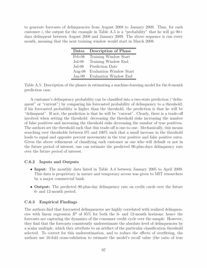
to generate forecasts of delinquencies from August 2008 to January 2009. Thus, for eachcustomer i, the output for the example in Table A.5 is a “probability” that he will go 90+days delinquent between August 2008 and January 2009. The above sequence is run everymonth, meaning that the next training window would start in March 2008.
Dates Description of Phase
Feb-08 Training Window StartJul-08 Training Window EndJul-08 Prediction DateAug-08 Evaluation Window StartJan-09 Evaluation Window End
Table A.5: Description of the phases in estimating a machine-learning model for the 6-monthprediction case.
A customer’s delinquency probability can be classified into a two-state prediction (“delin-quent” or “current”) by comparing his forecasted probability of delinquency to a threshold:if his forecasted probability is higher than the threshold, the prediction is that he will be“delinquent”. If not, the prediction is that he will be “current”. Clearly, there is a trade-offinvolved when setting the threshold: decreasing the threshold risks increasing the numberof false positives and increasing the threshold risks decreasing the number of true positives.The authors set the threshold such that this trade-off is one-to-one. Mechanically, this meanssearching over thresholds between 0% and 100% such that a small increase in the thresholdleads to equal and opposite percent movements in the true positive and false positive rates.Given the above refinement of classifying each customer as one who will default or not inthe future period of interest, one can estimate the predicted 90-plus-days delinquency rateover the future period of interest.
C.6.2 Inputs and Outputs
• Input: The monthly data listed in Table A.4 between January 2005 to April 2009.This data is proprietary in nature and temporary access was given to MIT researchersby a major commercial bank.
• Output: The predicted 90-plus-day delinquency rate on credit cards over the future6- and 12-month period.
C.6.3 Empirical Findings
The authors find that forecasted delinquencies are highly correlated with realized delinquen-cies with linear regression R2 of 85% for both the 6- and 12-month horizons; hence theforecasts are capturing the dynamics of the consumer credit cycle over the sample. However,they find that the forecasts consistently underestimate the absolute level of delinquencies bya scalar multiple, which they attribute to an artifact of the particular classification thresholdselected. To correct for this underestimation, and to reduce the effects of overfitting, theauthors use 10-fold cross-validation to estimate the model’s recall value (the ratio of true
97

negatives to the sum of true negatives and false positives). For a given training window, thisconsists of stratifying the dataset into 10 bins, using 9 of them for training of the model andthe remaining one for testing, and repeating this step 9 times using a different set of binsfor testing and training. The model’s recall value is estimated by averaging the 10 resultingrecall values. After obtaining the model’s recall value for a given horizon, the authors mul-tiply the forecasted default rate for that horizon by the reciprocal of this estimated recallrate. This is reasonably successful in correcting the underestimation bias, yielding forecaststhat are accurate both in terms of level and dynamics.
C.7 Principal Components Analysis
Kritzman, Li, Page, and Rigobon (2010) propose to measure systemic risk via the AbsorptionRatio (AR), which they define as the fraction of the total variance of a set of asset returnsexplained or “absorbed” by a fixed number of eigenvectors. The absorption ratio captures theextent to which markets are unified or tightly coupled. When markets are tightly coupled,they become more fragile in the sense that negative shocks propagate more quickly andbroadly than when markets are loosely linked. The authors apply their AR analysis toseveral broad markets, introduce a standardized measure of shifts in the AR, and analyzehow these shifts relate to changes in asset prices and financial turbulence.
C.7.1 Definition
In order to calculate the AR at a given time, the N × N covariance matrix of the N assetreturns is needed. Mathematically, the AR is defined as:
AR =
∑n
i=1 σ2Ei
∑nj=1 σ
2aj
(A.58)
where:
n = number of eigenvectors used in calculating AR
σ2Ei
= variance of eigenvector i
σ2aj
= variance of asset j
A high value for the absorption ratio corresponds to a high level of systemic risk because itimplies the sources of risk are more unified. A low absorption ratio indicates less systemicrisk because it implies the sources of risk are more disparate. High systemic risk does notnecessarily lead to asset depreciation or financial turbulence. It is simply an indication ofmarket fragility in the sense that a shock is more likely to propagate quickly and broadlywhen sources of risk are tightly coupled.
In order to estimate the AR, the authors use a 500-day window to estimate the covariancematrix and eigenvectors, and fix the number of eigenvectors at approximately 1/5th thenumber of assets. It should be noted that an eigenvector may or may not be associatedwith an observable financial variable; it may reflect a combination of several influences that
98
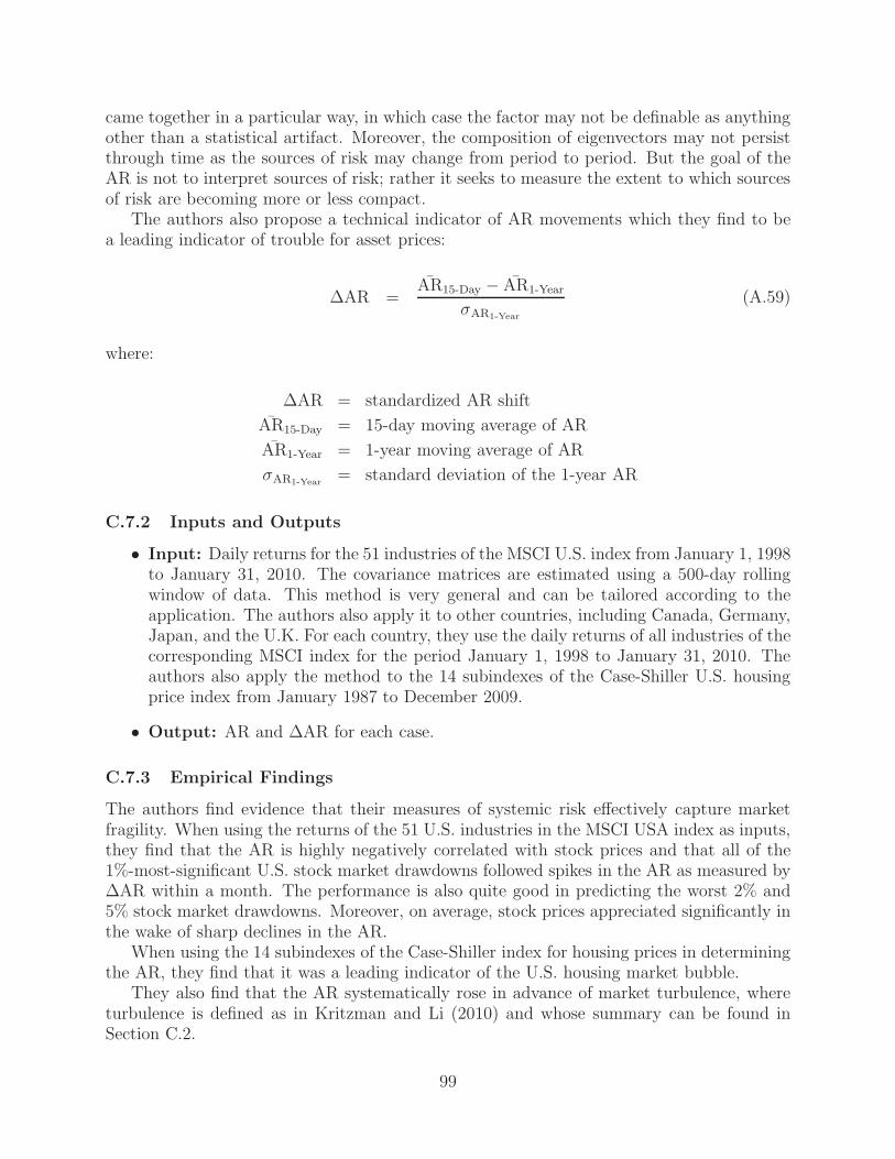
came together in a particular way, in which case the factor may not be definable as anythingother than a statistical artifact. Moreover, the composition of eigenvectors may not persistthrough time as the sources of risk may change from period to period. But the goal of theAR is not to interpret sources of risk; rather it seeks to measure the extent to which sourcesof risk are becoming more or less compact.
The authors also propose a technical indicator of AR movements which they find to bea leading indicator of trouble for asset prices:
∆AR =AR15-Day − AR1-Year
σAR1-Year
(A.59)
where:
∆AR = standardized AR shift
AR15-Day = 15-day moving average of AR
AR1-Year = 1-year moving average of AR
σAR1-Year= standard deviation of the 1-year AR
C.7.2 Inputs and Outputs
• Input: Daily returns for the 51 industries of the MSCI U.S. index from January 1, 1998to January 31, 2010. The covariance matrices are estimated using a 500-day rollingwindow of data. This method is very general and can be tailored according to theapplication. The authors also apply it to other countries, including Canada, Germany,Japan, and the U.K. For each country, they use the daily returns of all industries of thecorresponding MSCI index for the period January 1, 1998 to January 31, 2010. Theauthors also apply the method to the 14 subindexes of the Case-Shiller U.S. housingprice index from January 1987 to December 2009.
• Output: AR and ∆AR for each case.
C.7.3 Empirical Findings
The authors find evidence that their measures of systemic risk effectively capture marketfragility. When using the returns of the 51 U.S. industries in the MSCI USA index as inputs,they find that the AR is highly negatively correlated with stock prices and that all of the1%-most-significant U.S. stock market drawdowns followed spikes in the AR as measured by∆AR within a month. The performance is also quite good in predicting the worst 2% and5% stock market drawdowns. Moreover, on average, stock prices appreciated significantly inthe wake of sharp declines in the AR.
When using the 14 subindexes of the Case-Shiller index for housing prices in determiningthe AR, they find that it was a leading indicator of the U.S. housing market bubble.
They also find that the AR systematically rose in advance of market turbulence, whereturbulence is defined as in Kritzman and Li (2010) and whose summary can be found inSection C.2.
99

Another study which uses PCA as its primer is Billio, Getmansky, Lo, and Pelizzon(2010), which is presented in Section B.5. A good reference for more reading on the mathe-matics behind PCA is Jolliffe (2002).
D Stress Tests
Stress tests are a special case of forward-looking analysis with a significant role in systemicrisk monitoring. Stress testing is codified in regulation and international standards, includingthe Basel accord. Because the salient issues in stress testing are summarized in the maintext (see Section 2.5), we do not repeat that discussion here. Instead, we move directly to adescription of specific models.
D.1 GDP Stress Tests
Alfaro and Drehmann (2009) propose a macroeconomic stress test using a simple AR modelof GDP growth which is assumed to depend only on its past behavior. The reason the authorsfocus on GDP is they observe that domestic macroeconomic conditions as measured by GDPgrowth typically weaken ahead of banking crises. Furthermore, output drops substantiallyin nearly all of the observed crises once stress emerges. Their approach to stress testing usesthis as a starting point to construct GDP scenarios, independently of whether falls in outputtruly reflect or cause crises. Their guiding principle in creating their GDP shocks is thatstress scenarios should be severe yet plausible.
D.1.1 Definition
In defining crises, the authors rely on Reinhart and Rogoff (2008), who define the beginningof a crisis by the emergence of large-scale policy assistance or the default of important playersin the financial system.
The authors assume an AR model of GDP growth (to replicate the information availableto policymakers before a crisis, the authors estimate a different model for each crisis in eachcountry, using only data up to the crisis itself):
yt = ρ1yt−1 + ρ2yt−2 + εt (A.60)
where yt denotes the real GDP growth rate at time t. For each country, the BayesianInformation Criterion (BIC) is used in determining whether 1 or 2 lags should be used. Asa stress scenario, the authors use the worst negative forecast error of the above AR model,regardless of whether this coincided with a banking crisis or not. They then shock themodel in (A.60) with this very negative ε four quarters before the beginning of the crisis andcompare the maximum drop in GDP growth during the stress test with the maximum dropduring the actual episode. The maximum drop in GDP growth during a crisis is calculatedas the difference between the GDP growth four quarters prior to the crisis and the minimumGDP growth within two years after the crisis.
100
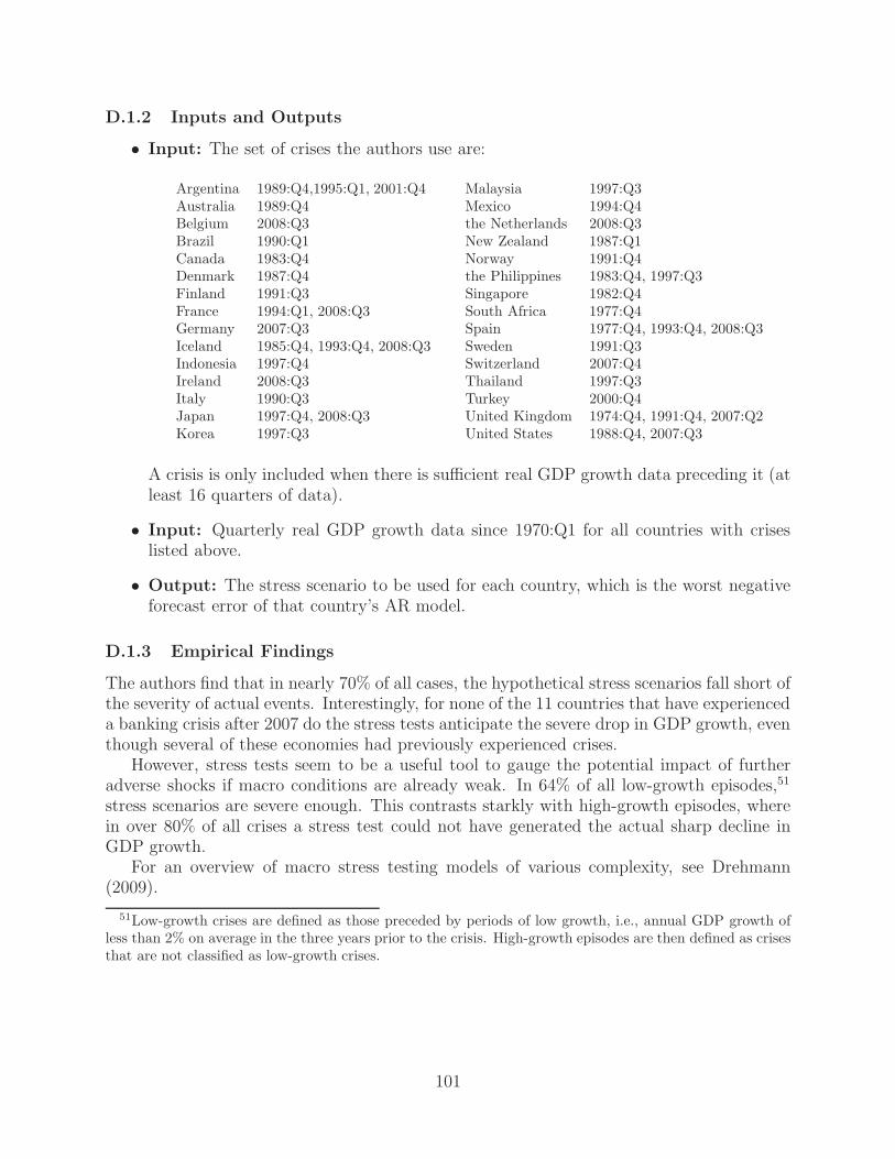
D.1.2 Inputs and Outputs
• Input: The set of crises the authors use are:
Argentina 1989:Q4,1995:Q1, 2001:Q4 Malaysia 1997:Q3Australia 1989:Q4 Mexico 1994:Q4Belgium 2008:Q3 the Netherlands 2008:Q3Brazil 1990:Q1 New Zealand 1987:Q1Canada 1983:Q4 Norway 1991:Q4Denmark 1987:Q4 the Philippines 1983:Q4, 1997:Q3Finland 1991:Q3 Singapore 1982:Q4France 1994:Q1, 2008:Q3 South Africa 1977:Q4Germany 2007:Q3 Spain 1977:Q4, 1993:Q4, 2008:Q3Iceland 1985:Q4, 1993:Q4, 2008:Q3 Sweden 1991:Q3Indonesia 1997:Q4 Switzerland 2007:Q4Ireland 2008:Q3 Thailand 1997:Q3Italy 1990:Q3 Turkey 2000:Q4Japan 1997:Q4, 2008:Q3 United Kingdom 1974:Q4, 1991:Q4, 2007:Q2Korea 1997:Q3 United States 1988:Q4, 2007:Q3
A crisis is only included when there is sufficient real GDP growth data preceding it (atleast 16 quarters of data).
• Input: Quarterly real GDP growth data since 1970:Q1 for all countries with criseslisted above.
• Output: The stress scenario to be used for each country, which is the worst negativeforecast error of that country’s AR model.
D.1.3 Empirical Findings
The authors find that in nearly 70% of all cases, the hypothetical stress scenarios fall short ofthe severity of actual events. Interestingly, for none of the 11 countries that have experienceda banking crisis after 2007 do the stress tests anticipate the severe drop in GDP growth, eventhough several of these economies had previously experienced crises.
However, stress tests seem to be a useful tool to gauge the potential impact of furtheradverse shocks if macro conditions are already weak. In 64% of all low-growth episodes,51
stress scenarios are severe enough. This contrasts starkly with high-growth episodes, wherein over 80% of all crises a stress test could not have generated the actual sharp decline inGDP growth.
For an overview of macro stress testing models of various complexity, see Drehmann(2009).
51Low-growth crises are defined as those preceded by periods of low growth, i.e., annual GDP growth ofless than 2% on average in the three years prior to the crisis. High-growth episodes are then defined as crisesthat are not classified as low-growth crises.
101

D.2 Lessons from the SCAP
Hirtle, Schuermann, and Stiroh (2009) describe some of the lessons learned from the Su-pervisory Capital Assessment Program (SCAP) or “stress tests” conducted by the FederalReserve in 2009–2010 on the 19 largest U.S. bank holding companies. The SCAP is one ex-ample of how the macro- and microprudential perspectives can be joined to create a strongersupervisory framework that addresses a wider range of supervisory objectives. The authorsreview the key features of the SCAP and discuss how they can be leveraged to improve banksupervision in the future.
The goal of macroprudential regulation is to reduce the probability of distress for theentire financial system when that distress has the potential to adversely impact the realeconomy. This link incorporates a host of potential channels including interdependenceand linkages among large financial firms through clearing and settlement systems, commonexposures, collective or “herd” behavior, and market failures such as externalities or moralhazard, all of which have the potential to amplify shocks and spill over to the real economy.Supervisors then have an incentive to “lean against the wind” of broader destabilizing forceswith countercyclical pressures. The SCAP had important features of macroprudential andmicroprudential supervision. From the macroprudential perspective, the SCAP was a top-down analysis of the largest bank holding companies (BHCs), representing a majority ofthe U.S. banking system, with an explicit goal to facilitate aggregate lending. The SCAPapplied a common, probabilistic scenario analysis for all participating BHCs and lookedbeyond the traditional accounting-based measures to determine the needed capital buffer.The macroprudential goal was to credibly reduce the probability of the tail outcome, but theanalysis began at the microprudential level with detailed and idiosyncratic data on the risksand exposures of each participating BHC. This firm-specific, granular data allowed tailoredanalysis that led to differentiation and BHC-specific policy actions.
Supervisors collected significant amounts of confidential data about BHCs’ loan and se-curities portfolios, trading accounts, derivatives positions, and revenue and expense sources.Using these data, supervisors were able to develop independent estimates of losses and rev-enues for the participating firms. The final SCAP projections of losses, revenues, and reserveneeds were developed through review and analysis by more than 150 senior supervisors, exam-iners, economists, financial analysts, and experts in law, accounting, and regulatory capitalat the supervisory agencies.
Some other key elements of the SCAP that made it successful include comprehensivecoverage of participating BHCs; use of a consistent framework across firms; use of multiple,independent estimates of loss and revenue, rather than a single model or approach; trans-parency about the process and results; and a clear set of goals and resulting policy actionsthat were articulated in advance and well-understood by all parties.
D.3 A 10-by-10-by-10 Approach
In Duffie’s (2011) proposal, a regulator would collect and analyze information concerningthe exposures of N “important” institutions to M defined stress scenarios. For each stressscenario, an important institution would report its gain or loss, in total, and with respect toits contractual positions with each of the entities for which its exposure, for that scenario,is among the K greatest in magnitude relative to all counterparties. Those counterparties
102

would be identified, stress by stress. The N significant entities would be those identified bythe Financial Stability Board.
With this approach, the joint exposure of the system to particular stress tests and partic-ular entities (or chains of entities) could be clarified as a result. New systemically importantentities might emerge from the analysis because some of the K entities to whom a reportingimportant institution has its largest exposures, for a given stress scenario, need not be amongthe original N reporting important institutions, but could become identified as systemicallyvulnerable as a result of the analysis.
The types of stresses that would be explored should involve scenarios that are not coveredby delta-based hedging and are conjectured to have potential systemic importance. The sizesof the defined stresses should therefore capture movements that are extreme but plausible.The asset classes covered by the scenarios should be broad enough to incorporate likelyincreases in cross-asset return correlations in crisis settings.
Illustrative examples of such stress scenarios that the author gives are:
1. The default of a single entity.2. A 4% simultaneous change in all credit yield spreads.3. A 4% shift of the U.S.-dollar yield curve.4. A 25% change in the value of the dollar relative to a basket of major currencies.5. A 25% change in the value of the Euro relative to a basket of major currencies.6. A 25% change in a major real estate index.7. A 50% simultaneous change in the prices of all energy-related commodities.8. A 50% change in a global equities index.
The results of such a survey can help increase the transparency of hedge funds and howthey play into the systemic risk in the financial sector. Theoretically, if a hedge fund failureaffects many banks, that hedge fund poses a large systemic risk. Furthermore, if a hedgefund is consistently one of the top gain/loss counterparties with important institutions, itmust be systemically important.
A major shortcoming of this approach is that it will miss widely dispersed potentialsources of systemic risk that do not flow through major financial institutions. For example,the U.S. Savings and Loans Crisis probably did not register directly measurable stress tojust a handful of important financial institutions.
D.3.1 Inputs and Outputs
The author did not actually run any simulations, he just outlined the basic idea. We sum-marize the inputs and outputs that would be needed to implement his proposal.
• Input: The M stress scenarios to be considered by the N important institutions. Theauthor gives examples of such scenarios (see the previous section).
• Input: The responses of each of the N important institutions to each of the M stressscenarios. This is survey data and could be made a mandatory reporting requirementfor the important institutions on a quarterly basis.
• Output: For each important institution and for each stress scenario, a list of the topK counterparties that would suffer.
103
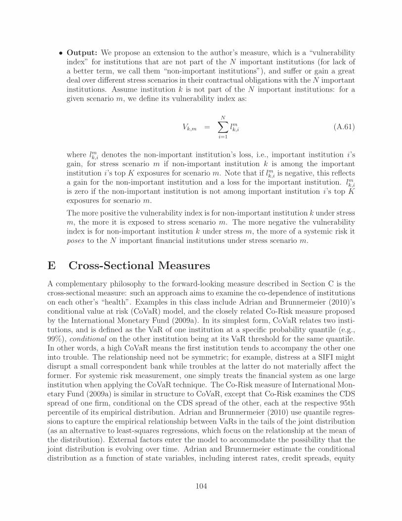
• Output: We propose an extension to the author’s measure, which is a “vulnerabilityindex” for institutions that are not part of the N important institutions (for lack ofa better term, we call them “non-important institutions”), and suffer or gain a greatdeal over different stress scenarios in their contractual obligations with theN importantinstitutions. Assume institution k is not part of the N important institutions: for agiven scenario m, we define its vulnerability index as:
Vk,m =N∑
i=1
lmk,i (A.61)
where lmk,i denotes the non-important institution’s loss, i.e., important institution i ’sgain, for stress scenario m if non-important institution k is among the importantinstitution i ’s top K exposures for scenario m. Note that if lmk,i is negative, this reflectsa gain for the non-important institution and a loss for the important institution. lmk,iis zero if the non-important institution is not among important institution i ’s top Kexposures for scenario m.
The more positive the vulnerability index is for non-important institution k under stressm, the more it is exposed to stress scenario m. The more negative the vulnerabilityindex is for non-important institution k under stress m, the more of a systemic risk itposes to the N important financial institutions under stress scenario m.
E Cross-Sectional Measures
A complementary philosophy to the forward-looking measure described in Section C is thecross-sectional measure: such an approach aims to examine the co-dependence of institutionson each other’s “health”. Examples in this class include Adrian and Brunnermeier (2010)’sconditional value at risk (CoVaR) model, and the closely related Co-Risk measure proposedby the International Monetary Fund (2009a). In its simplest form, CoVaR relates two insti-tutions, and is defined as the VaR of one institution at a specific probability quantile (e.g.,99%), conditional on the other institution being at its VaR threshold for the same quantile.In other words, a high CoVaR means the first institution tends to accompany the other oneinto trouble. The relationship need not be symmetric; for example, distress at a SIFI mightdisrupt a small correspondent bank while troubles at the latter do not materially affect theformer. For systemic risk measurement, one simply treats the financial system as one largeinstitution when applying the CoVaR technique. The Co-Risk measure of International Mon-etary Fund (2009a) is similar in structure to CoVaR, except that Co-Risk examines the CDSspread of one firm, conditional on the CDS spread of the other, each at the respective 95thpercentile of its empirical distribution. Adrian and Brunnermeier (2010) use quantile regres-sions to capture the empirical relationship between VaRs in the tails of the joint distribution(as an alternative to least-squares regressions, which focus on the relationship at the mean ofthe distribution). External factors enter the model to accommodate the possibility that thejoint distribution is evolving over time. Adrian and Brunnermeier estimate the conditionaldistribution as a function of state variables, including interest rates, credit spreads, equity
104

prices, and a volatility index. The International Monetary Fund (2009b) adopts a similarprocedure for their Co-Risk model, without credit spreads.52
E.1 CoVaR
Adrian and Brunnermeier (2010) propose to measure systemic risk via the conditional value-at-risk (CoVaR) of the financial system, conditional on institutions being in a state of dis-tress. An institution’s contribution to systemic risk is defined as the difference betweenCoVaR conditional on the institution being in distress and CoVaR in the median state ofthe institution. The CoVaR systemic risk measure is able to identify the risk on the systemby individually “systemically important” institutions, which are so interconnected and largethat they can cause negative risk spillover effects on others, as well as by smaller institutionsthat are “systemic” when acting as part of a herd. Furthermore, CoVaR is a measure whichdoes not rely on contemporaneous price movements and thus can be used to anticipate sys-temic risk. The CoVaR measure captures institutional externalities such as “too big to fail”,“too interconnected to fail”, and crowded trade positions.
E.1.1 Definition
Recall that the value-at-risk of institution i at the q percentile is defined as:
Pr(X i ≤ VaRiq) = q (A.62)
where X i denotes the asset return value of institution i. Note that V aRiq is typically a
negative number. The VaR of institution j (or the financial system) conditional on theevent X i = V aRi
q, i.e., institution i’s asset-return attains its VaR value, is denoted by
CoVaRj|iq , where q is the quantile. Mathematically:
Pr(Xj ≤ CoVaRj|iq |X i = VaRi
q) = q . (A.63)
Institution i’s contribution to the risk of j is defined as:
∆CoVaRj|iq = CoVaRj|i
q − CoVaRj|i50% (A.64)
where CoVaRj|i50% denotes the VaR of j’s asset returns when i’s returns are at their median
(i.e. 50th percentile). In their paper, the authors focus on the case where j = system, i.e.,when the return of the portfolio of all financial institutions is at its VaR level. In this case,
52A conceptually closely related model is the distressed insurance premium (DIP) of Huang, Zhou, and Zhu(2009b), which measures the conditional expected shortfall (CoES) of an institution, conditional on systemicdistress. The DIP represents a hypothetical insurance premium against systemic distress, defined as totallosses exceeding a threshold level of 15% of total bank liabilities. The implementation differs significantlyfrom the CoVaR and Co-Risk models just described, however, and is based on ex ante default probabilitiesand forecast asset return correlations for individual banks, derived from market data including realized(high-frequency) correlations, interest rates, equity prices, and a volatility index.
105

the superscript j is dropped. Hence, ∆CoVaRi denotes the difference between the VaR ofthe financial system conditional on the distress of a particular financial institution i andthe VaR of the financial system conditional on the median state of the institution i. Thus,∆CoVaRi quantifies how much an institution adds to overall systemic risk.
Before discussing how to estimate CoVaR, we present how to estimate the market valueof asset returns for financial institutions. Denote by MEi
t the market value of institution i’stotal equity, and by LEV i
t the ratio of total book assets to book equity. The growth rate ofmarket valued total assets X i
t is given by:
X it =
MEit · LEV i
t − MEit−1 · LEV i
t−1
MEit−1 · LEV i
t−1
=Ai
t − Ait−1
Ait−1
(A.65)
where Ait = MEi
tLEV it . Essentially, (A.65) is just applying the market-to-book equity ratio
to transform book-valued assets into market valued assets.To capture the time variation in the joint distribution of X i and Xsystem, the condi-
tional distribution is estimated as a function of state variables. The following two quantileregressions are run on weekly data:
X it = αi + γiMt−1 + εit (A.66a)
Xsystemt = αsystem|i + βsystem|iX i
t + γsystem|iMt−1 + εsystem|it (A.66b)
where Mt denotes a vector of state variables described in Table A.6. A quantile regressionconsists of optimizing a modified function shown below for the quantile regression in (A.66a):
minαq,βq,γq
∑
t
q|X it − αq −Mt−1γq| if (X i
t − αq −Mt−1γq) ≥ 0
(1− q)|X it − αq −Mt−1γq| if (X i
t − αq −Mt−1γq) ≤ 0. (A.67)
The quantile regression for (A.66b) is analogous. Having estimated the quantile regressionparameters, the predicted values of VaR and CoVaR are:
VaRit = αi + γiMt−1 (A.68a)
CoVaRit = αsystem|i + βsystem|iVaRi
t + γsystem|iMt−1 . (A.68b)
Finally, ∆CoVaRit for each institution is calculated as:
∆CoVaRit(q) = CoVaRi
t(q)− CoVaRit(50%) (A.69)
= βsystem|i(VaRit(q)−VaRi
t(50%)) .
Thus, in order to estimate institution i’s contribution to systemic risk, ∆CoVaRit, the quantile
regressions in equation (A.66a) must be run twice: once for the desired q and once for q = 0.5.
106

Throughout the paper, the authors estimate ∆CoVaRit for both the q = 1% and the q = 5%
cases.
State Variables in Mt Source
VIX CBOE website
3M repo rate − 3M UST Bloomberg (repo rate)FRBNY site (T-bill rate)
Weekly change of 3M T-bill rate FRB H15 Release
Weekly Change in UST yield spread (10Y − 3M) FRB H15 Release
Weekly Change in credit spread (10Y BAA bonds − 10Y UST) FRB H15 Release
Weekly VW equity market return CRSP
1Y real estate sector return via- CRSP companies with-the VW average return of real estate companies SIC code 65–66
Table A.6: State variables used in CoVaR estimation.
E.1.2 Inputs and Outputs
The financial institutions on which the authors apply their CoVaR estimator are those in theCRSP database with two-digit SIC codes between 60 and 67 inclusive, indexed by PERMNO.Only firms with common shares are used.
• Input: Weekly data for the market value of equity for the institutions of interest forthe period 1986:Q1–2010:Q1. This data is taken from CRSP.
• Input: Data on the book value of assets and book value of equity for each institutionfor the period 1986:Q1–2010:Q1. From this data, the book leverage (LVG) can beestimated. This data is available quarterly from the Compustat database. Since thebook value data is quarterly, within a given quarter, the dynamics of X i
t are drivensolely by the dynamics of the market value of equity (see (A.65)).
Note that Xsystemt is simply the market capitalization weighted average of each insti-
tution’s asset returns.
• Input: The weekly data described in Table A.6.
• Input: The desired quantile; the authors use both 1% and 5%.
• Output: The marginal contribution of institution i to systemic risk, ∆CoVaRit(q) as
defined in equation (A.69).
• Output: The VaR of institution j conditional on institution i being in distress. Thiscan be found by running the quantile regressions system in (A.66) and evaluating(A.68) and (A.69) where system is replaced by j.
107

E.1.3 Empirical Findings
The authors find that, across institutions, there is only a very loose link between an institu-tion’s VaR and its contribution to systemic risk as measured by CoVaRi. Hence, imposingfinancial regulation that is solely based on the individual risk of an institution in isolationmight not be sufficient to insulate the financial sector against systemic risk.
The authors run regression analyses in order to examine what firm characteristics aregood predictors of future CoVaR. They find that firms with higher leverage, more maturitymismatch, and larger size tend to be associated with larger systemic risk contributions onequarter, one year, and two years later, both at the 1% and the 5% levels.
They then use these firm variables to predict “forward ∆CoVaR” two years into thefuture, and find that it is negatively correlated with contemporaneous ∆CoVaR, i.e., theresult of estimating it via the methods outlined in Section E.1.1. Thus, macroprudentialregulation based on the “forward ∆CoVaR” is countercyclical.
For a detailed exposition of quantile regression techniques, see Koenker (2005) and foran intuitive exposition, see Koenker and Hallock (2001).
E.2 Distressed Insurance Premium
The Distressed Insurance Premium (DIP) is proposed as an ex ante systemic risk metric byHuang, Zhou, and Zhu (2009b) and it represents a hypothetical insurance premium againsta systemic financial distress, defined as total losses that exceed a given threshold, say 15%,of total bank liabilities. The methodology is general and can apply to any pre-selectedgroup of firms with publicly tradable equity and CDS contracts. Each institution’s marginalcontribution to systemic risk is a function of its size, probability of default (PoD), and assetcorrelation. The last two components need to be estimated from market data.
E.2.1 Definition
The PoD uses CDS quotes referring to 5-year, senior unsecured debt with no-restructuringclauses that are U.S.-dollar denominated. The authors use end-of-week observations toconstruct weekly CDS data. The 1-year risk-neutral PoD of the bank is given by:
PoDi,t =atsi,t
atLGDi,t + btsi,t(A.70)
where at =∫ t+T
te−rx dx and bt =
∫ t+T
txe−rx dx, LGD is the loss given default, si,t is the
CDS spread of bank i at time t, and r is the risk-free rate. The LGD is needed as an input:although one can use the Basel II recommendation of 55%, the authors choose to use theexpected LGD as reported by market participants who price and trade CDS contracts.
The next step is to estimate the correlation of the banks’ assets. The authors assumethat at frequencies less than 12 weeks, leverage is approximately constant and thus assetcorrelation can be proxied by equity correlation. They test the constant leverage hypothesisand find that it holds for 10 of the 12 banks in their sample. Using high-frequency tick-by-tickdata from the TAQ database, they estimate their measure of correlation as follows:
108
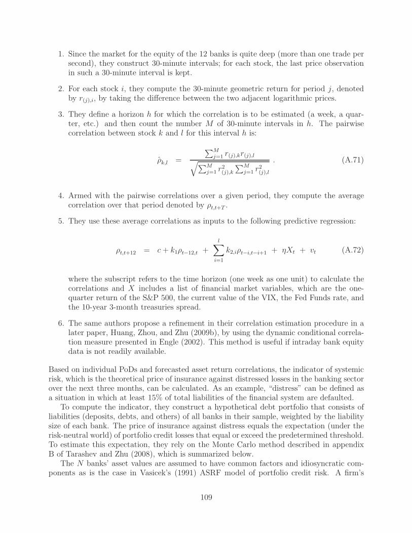
1. Since the market for the equity of the 12 banks is quite deep (more than one trade persecond), they construct 30-minute intervals; for each stock, the last price observationin such a 30-minute interval is kept.
2. For each stock i, they compute the 30-minute geometric return for period j, denotedby r(j),i, by taking the difference between the two adjacent logarithmic prices.
3. They define a horizon h for which the correlation is to be estimated (a week, a quar-ter, etc.) and then count the number M of 30-minute intervals in h. The pairwisecorrelation between stock k and l for this interval h is:
ρk,l =
∑Mj=1 r(j),kr(j),l
√
∑Mj=1 r
2(j),k
∑Mj=1 r
2(j),l
. (A.71)
4. Armed with the pairwise correlations over a given period, they compute the averagecorrelation over that period denoted by ρt,t+T .
5. They use these average correlations as inputs to the following predictive regression:
ρt,t+12 = c + k1ρt−12,t +l∑
i=1
k2,iρt−i,t−i+1 + ηXt + vt (A.72)
where the subscript refers to the time horizon (one week as one unit) to calculate thecorrelations and X includes a list of financial market variables, which are the one-quarter return of the S&P 500, the current value of the VIX, the Fed Funds rate, andthe 10-year 3-month treasuries spread.
6. The same authors propose a refinement in their correlation estimation procedure in alater paper, Huang, Zhou, and Zhu (2009b), by using the dynamic conditional correla-tion measure presented in Engle (2002). This method is useful if intraday bank equitydata is not readily available.
Based on individual PoDs and forecasted asset return correlations, the indicator of systemicrisk, which is the theoretical price of insurance against distressed losses in the banking sectorover the next three months, can be calculated. As an example, “distress” can be defined asa situation in which at least 15% of total liabilities of the financial system are defaulted.
To compute the indicator, they construct a hypothetical debt portfolio that consists ofliabilities (deposits, debts, and others) of all banks in their sample, weighted by the liabilitysize of each bank. The price of insurance against distress equals the expectation (under therisk-neutral world) of portfolio credit losses that equal or exceed the predetermined threshold.To estimate this expectation, they rely on the Monte Carlo method described in appendixB of Tarashev and Zhu (2008), which is summarized below.
The N banks’ asset values are assumed to have common factors and idiosyncratic com-ponents as is the case in Vasicek’s (1991) ASRF model of portfolio credit risk. A firm’s
109

LGD is assumed to be independent of the factors underlying the stochastic process of itsassets and the distribution of LGDs is identical across exposures. The simulation of portfoliocredit losses can be divided into two parts: the first part calculates the probability distribu-tion of joint defaults and the second part incorporates the LGD distribution to derive theprobability distribution of portfolio losses.
Part 1:
1. Using the N × 1 vector of PoDs and the assumption that asset returns are distributedas standard normal variables, they obtain an N × 1 vector of default thresholds.
2. They draw an N × 1 vector from N standard normal random variables which are allassumed to have a pairwise correlation equal to the forward looking average correlationmeasure estimated in (A.72). The number of entries in this vector, which are smallerthan the corresponding default threshold, is the number of simulated defaults for theparticular draw.
3. The above step is repeated 500,000 times to derive the probability distribution of thenumber of defaults, Pr(number of defaults = k), where k = 0, 1, . . . , N .
Part 2:
1. For a given number of defaults k, they draw LGDs for the default exposure 1,000 timesfrom a triangular distribution centered at 0.55 (Basel II recommendation) with range[0.1, 1] and calculate the conditional loss distribution Pr(TL|k defaults).
2. The above step is done for each k = 1, . . . , N . Then, they are able to calculate theunconditional probability distribution of portfolio credit losses. Specifically:
Pr(TL) =∑
k
Pr(TL|k defaults) Pr(k defaults) . (A.73)
3. Armed with the unconditional distribution of losses, they can then calculate the prob-ability of the event that the total losses are above 15% of the total banking sectorliabilities; to get the DIP, we then multiply the above probability with the expectedlosses conditional on the event that the losses are above 15% of the total banking sectorliabilities.
E.2.2 Extensions
In Huang, Zhou, and Zhu (2009b), the authors propose two extensions of the DIP method-ology used in Huang, Zhou, and Zhu (2009a) to analyze the sources of systemic risk: usingobjective probabilities of defaults instead of risk-neutral ones and identifying the systemicrisk contribution of each institution.
For the former case, the systemic risk indicator uses PoDs that are estimated by usingthose supplied by Moody’s KMV-EDF for each institution; these PoDs reflect the objectiveprobability of default. The resulting DIP quantifies the contribution from the expected
110

actual defaults, and the difference between the market DIP (risk-neutral PoD case) andthe actuarial DIP (objective PoD case) quantifies the contribution from the risk premiacomponents.
For the latter case, the authors try to estimate the loss arising from a bank’s default,conditional on the occurrence of the distress scenario where at least 15% of total liabilitiesare defaulted upon. Because systemic events are rare, the authors use importance sampling(see Glasserman and Li (2005)) to simulate these events. For the 22 bank portfolios intheir sample, they generate 200,000 importance-sampling simulations of default scenarios(defaults or not), and for each scenario they generate 100 simulations of LGDs drawn fromthe distribution used in step 1 of part 2 of the simulation presented in Section E.2.1. Based onthese simulation results, they estimate each bank’s systemic risk contribution by calculatingthe expected loss of the bank conditional on total losses exceeding 15% of total liabilities.
E.2.3 Inputs and Outputs
• Input: To calculate the risk-neutral PoDs, daily 5-year CDS spread data for each bankare obtained from Markit; end-of-week observations are used to construct the weeklyCDS dataset from January 2001 to December 2008.
• Input: The expected LGDs for each firm. The authors use expected LGDs as reportedby market participants who price and trade CDS contracts. Alternatively, one can usethe Basel II recommendation of 55%.
• Input: The objective PoDs are supplied by Moody’s-KMV.
• Input: The raw high-frequency equity price data from the TAQ database to construct30-minute interval prices in order to estimate pairwise correlations used in (A.72).Only the data during normal market hours (9:30am–4:00pm) are used.
• Input: Histories of the one-quarter return of the S&P 500 (from Bloomberg), theVIX (from Bloomberg), the Fed Funds rate (Fed’s H15 Release), and the 10-year 3-month Treasuries spread (Fed’s H15 Release) to use as inputs in estimating the forwardlooking average correlation in (A.72).
• Output The DIP systemic risk indicator resulting from the simulation presented inSection E.2.1.
E.2.4 Empirical Findings
The authors run the DIP indicator over time and find that the DIP per unit of overallliabilities started at 10 basis points in the first half of 2001, increased, and reached a peakof about 35 basis points in the second half of 2002, when high corporate defaults werereported. The indicator then trended downward and reached its lowest level in late 2006 andearly 2007. Since August 2007, the indicator rose sharply, peaking around March 2008, anddropped dramatically after the Federal Reserve facilitated the acquisition of Bear Stearns byJ.P. Morgan Chase. They also find that most of its movement was impacted by the changingPoDs although the correlation measure also plays a role.
111

In terms of the extensions presented in Huang, Zhou, and Zhu (2009b), the authors findthat the actuarial DIP, i.e., using objective PoDs, is much smaller than the market DIPduring the crisis. This suggests that during a crisis period, the bailout cost of a market-based solution is much larger than that justified by an objective assessment of the defaultlosses due to increased risk aversion and decreased liquidity.
In terms of estimating banks’ individual contributions to systemic risk, they find thattypically, the largest banks coincide with the largest systemic risk contributors.
E.3 Co-Risk
The “Co-Risk” measure, first proposed in the IMF’s 2009 Global Financial Stability Review(International Monetary Fund, 2009a), examines the co-dependence between the CDS of var-ious financial institutions. It is more informative than unconditional risk measures becauseit provides a market assessment of the proportional increase in a firm’s credit risk induced,directly and indirectly, from its links to another firm. Note that the approach used is basedon quantile regression, a concept also used in CoVaR (see Adrian and Brunnermeier (2010),a summary of which is presented in Section E.1). The quantile regression approach permitsa more accurate estimation of the co-movements of financial institutions’ risk factors (orco-risk estimates) under distress, taking into account their nonlinear relationship.
E.3.1 Definition
The authors used daily five-year-maturity CDS spreads for a variety of financial institutionsfrom July 1, 2003 to September 12, 2008. Intuitively, when an institution’s CDS spreads arein their 5th quantile (the left tail of their distribution), this suggests that these institutionsare experiencing an extremely benign regime, and when the CDS spreads are at their 95th
quantile (the right tail of their distribution), this suggests a distress regime. Mathematically,the daily frequency quantile regression the authors run is:
CDSi,t = αiq +
K∑
m=1
βiq,mRm,t + βi
q,jCDSj,t + εi,t (A.74)
where CDSi,t is the CDS spread of institution i on day t, Rm,t is the value of risk factor m attime t, and q denotes the quantile. The parameter estimates, βi
q,j, provide a measure of howfirm j affects the credit risk of firm i (directly and indirectly) at different quantiles. TableA.7 presents the set of risk factors Rm that the authors use. Mathematically, the quantileregression consists of optimizing the function:
minαiq ,β
iq,m,βi
q,j
∑
t
ρq
(
CDSi,t − αiq −
K∑
m=1
βiq,mRm,t − βi
q,jCDSj,t
)
(A.75)
112
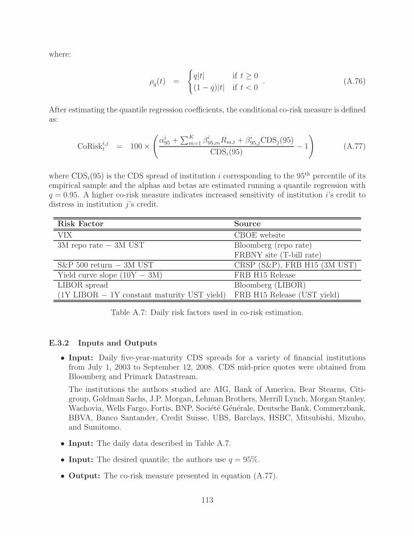
where:
ρq(t) =
q|t| if t ≥ 0
(1− q)|t| if t < 0. (A.76)
After estimating the quantile regression coefficients, the conditional co-risk measure is definedas:
CoRiski,jt = 100×(
αi95 +
∑K
m=1 βi95,mRm,t + βi
95,jCDSj(95)
CDSi(95)− 1
)
(A.77)
where CDSi(95) is the CDS spread of institution i corresponding to the 95th percentile of itsempirical sample and the alphas and betas are estimated running a quantile regression withq = 0.95. A higher co-risk measure indicates increased sensitivity of institution i’s credit todistress in institution j’s credit.
Risk Factor Source
VIX CBOE website3M repo rate − 3M UST Bloomberg (repo rate)
FRBNY site (T-bill rate)S&P 500 return − 3M UST CRSP (S&P), FRB H15 (3M UST)Yield curve slope (10Y − 3M) FRB H15 ReleaseLIBOR spread Bloomberg (LIBOR)(1Y LIBOR − 1Y constant maturity UST yield) FRB H15 Release (UST yield)
Table A.7: Daily risk factors used in co-risk estimation.
E.3.2 Inputs and Outputs
• Input: Daily five-year-maturity CDS spreads for a variety of financial institutionsfrom July 1, 2003 to September 12, 2008. CDS mid-price quotes were obtained fromBloomberg and Primark Datastream.
The institutions the authors studied are AIG, Bank of America, Bear Stearns, Citi-group, Goldman Sachs, J.P. Morgan, Lehman Brothers, Merrill Lynch, Morgan Stanley,Wachovia, Wells Fargo, Fortis, BNP, Societe Generale, Deutsche Bank, Commerzbank,BBVA, Banco Santander, Credit Suisse, UBS, Barclays, HSBC, Mitsubishi, Mizuho,and Sumitomo.
• Input: The daily data described in Table A.7.
• Input: The desired quantile; the authors use q = 95%.
• Output: The co-risk measure presented in equation (A.77).
113

E.3.3 Empirical Findings
The authors find that in March 2008, when Citigroup’s CDS spreads were at their 95th
percentile, this would have led to an increase of 135% in Bear Stearns’ CDS spread and103% in Lehman’s CDS spread. Furthermore, the risk of Bear Stearns conditional on therisk of AIG is 248% higher than that corresponding to the 95th percentile of Bear Stearns’empirical distribution. Thus, these results suggest that AIG, Bear Stearns, and Lehman,should have been closely monitored in March 2008.
The authors also find that in March 2008, the conditional co-risk of AIG and Lehmanto the rest of the institutions in the sample were, on average, 11% and 24%, respectively.However, on September 12, 2008, these estimates jumped to 30% and 36%, respectively, thushighlighting the increased systemic importance of these institutions at the peak of the crisis.
A more detailed exposition of the co-risk measure can be found in Chan-Lau (2009).For a detailed exposition of quantile regression techniques, see Koenker (2005) and for anintuitive exposition, see Koenker and Hallock (2001).
E.4 Marginal and Systemic Expected Shortfall
Acharya, Pedersen, Philippon, and Richardson (2010) argue that each financial institution’scontribution to systemic risk can be measured as its systemic expected shortfall (SES), i.e.,its propensity to be undercapitalized when the system as a whole is undercapitalized. SESis a theoretical construct and the authors use the following 3 measures to proxy it:
1. The outcome of stress tests performed by regulators. The SES metric of a firm hereis defined as the recommended capital that it was required to raise as a result of thestress test in February 2009.
2. The decline in equity valuations of large financial firms during the crisis, as measuredby their cumulative equity return from July 2007 to December 2008.
3. The widening of the credit default swap spreads of large financial firms as measuredby their cumulative CDS spread increases from July 2007 to December 2008.
Given these proxies, the authors seek to develop leading indicators which “predict” an insti-tution’s SES; these leading indicators are marginal expected shortfall (MES) and leverage(LVG). They provide a micro foundation argument about the theoretical relationship ofthese two indicators to SES, which we will not discuss here. The authors test MES andLVG with respect to their predictive power for the three SES proxies above and find decentpredictability.
E.4.1 Definition
A firm’s MES is defined as the average return of its equity (Rb) during the 5% worst days forthe overall market return (Rm), where the market is proxied by the CRSP Value WeightedIndex:
MESb =1
number of days
∑
t: system is in its 5% tail
Rbt . (A.78)
114
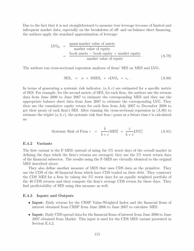
Due to the fact that it is not straightforward to measure true leverage because of limited andinfrequent market data, especially on the breakdown of off- and on-balance sheet financing,the authors apply the standard approximation of leverage:
LVGb =quasi-market value of assets
market value of equity
=book assets − book equity + market equity
market value of equity. (A.79)
The authors run cross-sectional regression analyses of firms’ SES on MES and LVG:
SESi = a + bMESi + cLVGi + εi . (A.80)
In terms of generating a systemic risk indicator, (a, b, c) are estimated for a specific metricof SES. For example, for the second metric of SES, for each firm, the authors use the returnsdata from June 2006 to June 2007 to estimate the corresponding MES and they use theappropriate balance sheet data from June 2007 to estimate the corresponding LVG. Theythen use the cumulative equity return for each firm from July 2007 to December 2008 toget their proxy of each firm’s SES. After running the cross-sectional regression in (A.80) toestimate the triplet (a, b, c), the systemic risk that firm i poses at a future time t is calculatedas:
Systemic Risk of Firm i =b
b+ cMESt
i +c
b+ cLVGt
i (A.81)
E.4.2 Variants
The first variant is the F-MES: instead of using the 5% worst days of the overall market indefining the days which the firm’s returns are averaged, they use the 5% worst return daysof the financial subsector. The results using the F-MES are virtually identical to the originalMES described above.
They also define another measure of MES that uses CDS data as the primitive. Theyuse the CDS of the 40 financial firms which have CDS traded on their debt. They constructthe CDS MES for a firm by taking the 5% worst days for an equally weighted portfolio ofthe 40 CDS returns and then compute the firm’s average CDS return for these days. Theyfind predictability of SES using this measure as well.
E.4.3 Inputs and Outputs
• Input: Daily returns for the CRSP Value-Weighted Index and the financial firms ofinterest obtained from CRSP from June 2006 to June 2007 to calculate MES.
• Input: Daily CDS spread data for the financial firms of interest from June 2006 to June2007 obtained from Markit. This input is used for the CDS MES variant presented inSection E.4.2.
115
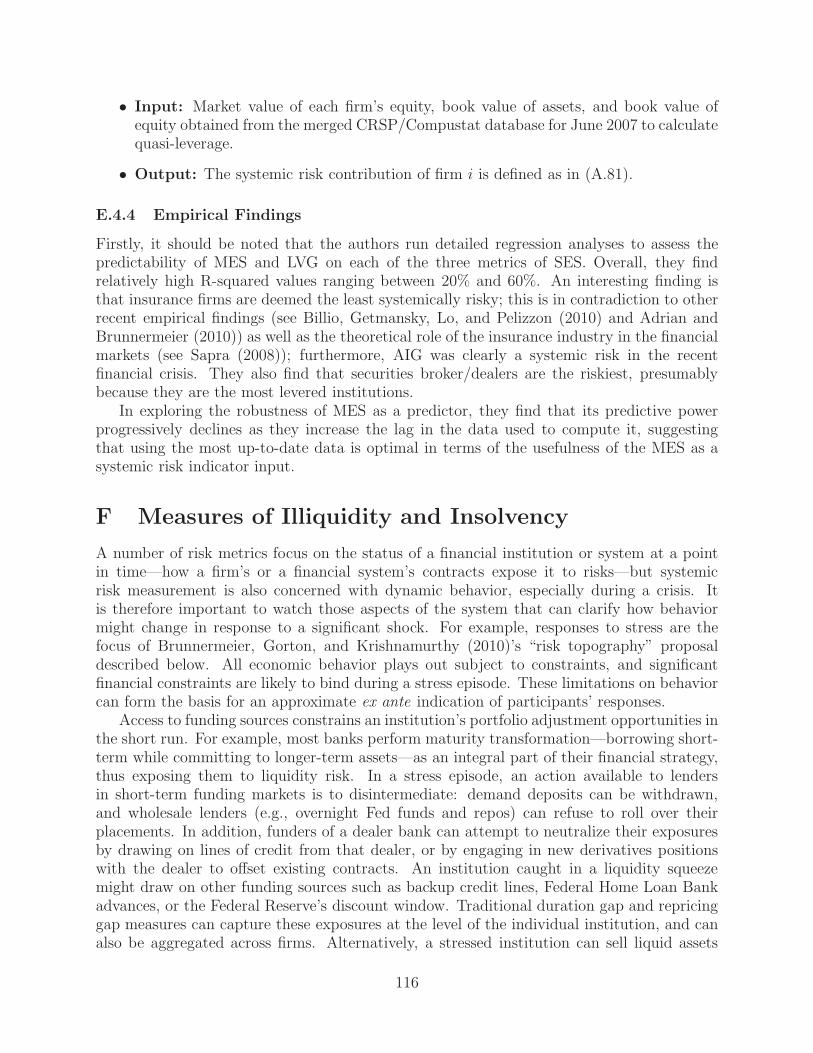
• Input: Market value of each firm’s equity, book value of assets, and book value ofequity obtained from the merged CRSP/Compustat database for June 2007 to calculatequasi-leverage.
• Output: The systemic risk contribution of firm i is defined as in (A.81).
E.4.4 Empirical Findings
Firstly, it should be noted that the authors run detailed regression analyses to assess thepredictability of MES and LVG on each of the three metrics of SES. Overall, they findrelatively high R-squared values ranging between 20% and 60%. An interesting finding isthat insurance firms are deemed the least systemically risky; this is in contradiction to otherrecent empirical findings (see Billio, Getmansky, Lo, and Pelizzon (2010) and Adrian andBrunnermeier (2010)) as well as the theoretical role of the insurance industry in the financialmarkets (see Sapra (2008)); furthermore, AIG was clearly a systemic risk in the recentfinancial crisis. They also find that securities broker/dealers are the riskiest, presumablybecause they are the most levered institutions.
In exploring the robustness of MES as a predictor, they find that its predictive powerprogressively declines as they increase the lag in the data used to compute it, suggestingthat using the most up-to-date data is optimal in terms of the usefulness of the MES as asystemic risk indicator input.
F Measures of Illiquidity and Insolvency
A number of risk metrics focus on the status of a financial institution or system at a pointin time—how a firm’s or a financial system’s contracts expose it to risks—but systemicrisk measurement is also concerned with dynamic behavior, especially during a crisis. Itis therefore important to watch those aspects of the system that can clarify how behaviormight change in response to a significant shock. For example, responses to stress are thefocus of Brunnermeier, Gorton, and Krishnamurthy (2010)’s “risk topography” proposaldescribed below. All economic behavior plays out subject to constraints, and significantfinancial constraints are likely to bind during a stress episode. These limitations on behaviorcan form the basis for an approximate ex ante indication of participants’ responses.
Access to funding sources constrains an institution’s portfolio adjustment opportunities inthe short run. For example, most banks perform maturity transformation—borrowing short-term while committing to longer-term assets—as an integral part of their financial strategy,thus exposing them to liquidity risk. In a stress episode, an action available to lendersin short-term funding markets is to disintermediate: demand deposits can be withdrawn,and wholesale lenders (e.g., overnight Fed funds and repos) can refuse to roll over theirplacements. In addition, funders of a dealer bank can attempt to neutralize their exposuresby drawing on lines of credit from that dealer, or by engaging in new derivatives positionswith the dealer to offset existing contracts. An institution caught in a liquidity squeezemight draw on other funding sources such as backup credit lines, Federal Home Loan Bankadvances, or the Federal Reserve’s discount window. Traditional duration gap and repricinggap measures can capture these exposures at the level of the individual institution, and canalso be aggregated across firms. Alternatively, a stressed institution can sell liquid assets
116

to raise cash. Small sales in active markets are unlikely to create large price movements: aseller would ordinarily work off a large position gradually to allow time for new bidders toarrive and replenish the rolls. In a crisis such patience is a luxury, and asset sales may eatdeeply into the set of buyers available immediately. Compounding the problem, potentialbuyers will exploit their bargaining power via lower offering prices if they detect the selleris liquidating under duress.
Leverage—the ratio of a position’s economic value to the size of the capital cushion sup-porting it—is an important feature of financial crises. Leverage simultaneously magnifiesthe percentage returns to capital investors and increases the risk of insolvency. Leverage isalso connected to liquidity and maturity through the financial structure of most intermedi-aries. A commercial bank, for example, invests in a diversified portfolio of illiquid, relativelylong-term loans, and issues liquid, short-term deposits. The law of large numbers createsthe predictability across both depositor withdrawals and loan defaults needed to make thisarrangement workable. McCulley (2010) emphasizes that “ex ante liquidity”—the notionthat a depositor could withdraw at will—is in relatively high demand, reducing the yieldbanks must pay on their demandable liabilities. This is a game of trust, because “ex-postliquidity” is not supportable on the same scale; a requirement to pay out depositor with-drawals in actuality will cause insolvency. To limit the externalities that come with failure,banks have recourse to deposit insurance and the central bank’s last-resort lending servicesto help insure the stability of this arrangement. However, this generates a moral hazardby insulating banks from their own liquidity risk, creating a need for prudential regulation.“Shadow” banks, on the other hand, also perform liquidity and maturity transformations,but position themselves to benefit from taxpayer-supported liquidity facilities without sub-jecting themselves to the countermanding regulatory regime.53 Financial Stability Board(2011) emphasizes that this can be profitable, but also destabilizing.
One way for banks (shadow or otherwise) to benefit from this moral hazard is throughexcessive leverage, which magnifies equity-holders’ positive returns, while imposing on tax-payers the losses in the event of bank failure. As a policy matter, it is insufficient to considerleverage only on a firm-by-firm basis: coordinated bank failures impose greater externalcosts than a single bank failure in isolation. Nijskens and Wagner (2011), for example, ex-amine the risk profiles of banks over the 1997–2006 period, finding that the securitization ofcommercial loans through collateralized loan obligations (CLOs) that reduced idiosyncraticbank risk simultaneously increased systemic risk by increasing betas and return correlationsacross institutions. Acharya, Pedersen, Philippon, and Richardson (2010) consider this sys-temic dimension with a collection of metrics that extend the familiar institution-level VaRand expected shortfall (ES) notion to capture an institution’s “systemic expected shortfall”(SES): its propensity to be undercapitalized when the system as a whole is undercapitalized.They also devise marginal expected shortfall (MES) and leverage metrics as early warningindicators of SES.
SES is a static measure, in the sense that it represents a measurable risk exposure of theinstitution at a particular point in time. Minsky (1982), in contrast, focuses on the endoge-nous dynamics of leverage. The crux of Minsky’s instability hypothesis is the tendency ofparticipants to increase their leverage over time. During episodes of rising asset prices, bothspeculation and increasing leverage are profitable ex post. (In a price bubble, this profitabil-
53Pozsar, Adrian, Ashcraft, and Boesky (2010) describe the shadow banking system in detail.
117
ity becomes self-fulfilling). Geanakoplos (2010) emphasizes the role of the marginal investor:above (below) her along the demand schedule are other buyers who are more (less) enthusi-astic about the security. Increasing leverage means that a smaller set of (more enthusiastic)investors can determine the price. In a boom, leverage and enthusiasm thus feed on eachother; the process is unsustainable if left unchecked. Eventually, the dynamic is reversed—perhaps by a random shock that imposes magnified losses on over-levered investors—anda self-reinforcing episode of price declines and deleveraging ensues. In short, the range ofpossible portfolio adjustments—which assets can be sold at what prices—is likely to changemarkedly during a stress episode. While some changes will only be apparent after the fact,other indicators—for example, based on bid-ask spreads, public limit order books, transac-tion volumes, and the characteristics of market-makers and other liquidity providers—canprovide ex ante evidence of deterioration in market quality. Hu, Pan, and Wang (2010) doc-ument this in the context of the market for U.S. Treasury securities. They derive a measureof market noise as the deviation of observed market yields on Treasury bonds from theirmodel-based yields derived from a daily estimate of the zero-coupon curve. They concludethat noise is typically quite low (and liquidity correspondingly high), enforced by arbitrage;however, noise spikes during crises as arbitrage capital exits the marketplace. Moreover,in a systemic crisis, many participants are likely to be liquidating simultaneously, furtherexacerbating short-term pressure on prices, while liquidity providers with thin capitalization(e.g., high-frequency traders) may exit the market altogether. Such coordinated behavior isthe essence of Pojarliev and Levich (2011)’s study of “crowded trades”, which uses a propri-etary high-frequency dataset of currency funds’ returns to examine the implications of theirtrading styles on price and correlation dynamics as well as the funds’ own profitability.54
Similar concerns arise in the other markets. Khandani and Lo (2011) propose two dis-tinct measures of equity market liquidity. They consider a contrarian trading strategy ofbuying losers and selling winners. This is essentially a market-making strategy that smoothstemporary supply-demand imbalances and compensates the trader for providing liquidity.Its profitability has been generally decreasing since the late 1990s, as increasing compe-tition in this strategy has reduced liquidity premiums. Their first measure examines theextent of high-frequency mean-reversion in transacted prices. Their second metric is “Kyle’slambda”, originally due to Kyle (1985), which measures liquidity via a regression estimateof the volume required to cause a one-dollar price movement.
Getmansky, Lo, and Makarov (2004) explore the sources of serial correlation in reportedhedge-fund returns, and conclude that the most likely explanation is illiquidity exposure andsmoothed returns. By definition, current prices in illiquid markets are frequently unavail-able or unreliable, forcing funds to report mark-to-model estimates that often rely linearextrapolation pricing methods. Serial correlation in observed returns is an artifact of thisautoregressive smoothing, and it thus offers a proxy measure for illiquidity.55
Counterparty insolvency also affects the set of portfolio-adjustment possibilities. Typi-
54They define four “style factors” as proxy measures for trading strategies and assess crowdedness as thenet proportion of funds in their sample exposed to each factor. They detect a significant connection betweencrowdedness and performance for currency funds.
55Chan, Getmansky, Haas, and Lo (2006b, 2006b) propose a related autocorrelation measure. They alsoestimate liquidation probabilities for hedge funds via logit regressions on samples of “live” and non-reportingfunds, and a regime-switching model (between high- and low-return states) for a variety of hedge-fund indicesthat can identify episodes of coordinated downturns.
118

cally, counterparties with short exposures to a defaulting firm do not lose everything on theirtransactions. For example, bilateral and multilateral netting agreements can sharply reducelosses given default, and many contracts include recourse to collateral in the event of coun-terparty default. Participation of individual contracts in netting or collateral arrangementsis in principle an observable fact. If collateral provisions exist, it is useful to know whethercollateral is pledged under a blanket lien or a specific lien, and what the collateral haircutsare. Similarly, for positions collateralized through margining agreements, it is valuable tomonitor the margin requirements, including procedures for calculating variation margin andmarking accounts to market. Haircuts and margins can change over time, and observationof these evolving values can provide valuable insights into creditworthiness. This is a centralelement of Brunnermeier, Gorton, and Krishnamurthy (2010)’s proposal to monitor systemicrisk via a two-step “risk topography” process. In the first step, regulators would accumulatea panel data set of participants’ individual risk exposures (changes in firm value) as wellas liquidity sensitivities (changes in “effective cash”) to various shock scenarios defined ona space of external factors. A key innovation is the introduction of a summable and state-contingent liquidity index for portfolio positions, to capture changes in fire-sale discountsor in collateral haircuts. The second step would aggregate firms’ individual valuation andliquidity responses into a system-wide picture of risks, where those exposures diversified inthe cross-section of firms should be of less concern that systemically concentrated exposures.Lastly, many positions are protected with third-party guarantors or in the CDS markets. Inthese cases, it is important to know the nature and amount of the protection, and to havea sense of the creditworthiness of the guarantor: wrong-way risk occurs when exposure toa counterparty correlates adversely with counterparty creditworthiness. For example, manyMBS bondholders discovered that the concentrated incidence of claims during the mortgagecrisis rendered guarantees from monoline subprime insurers unlikely to pay out preciselywhen the insured event occurred. If a guarantor’s or counterparty’s other exposures areobservable, then estimates of wrong-way risk become possible.
Liquidity and short-run portfolio flexibility present measurement challenges in manyways. For example, many markets do not publicly broadcast all the bids and offers—theeffective market depth—so that empirical studies have resorted to a variety of work-arounds.Hu, Pan, and Wang (2010) finesse the problem by tracking pricing “noise” as a signal ofthe absence from the market of arbitrage capital. Pojarliev and Levich (2011) assign hedgefunds to style categories to proxy for crowdedness in trading strategies. Khandani and Lo(2011) use market trading volume to help filter out the Kyle’s lambda metric for liquidity.Getmansky, Lo, and Makarov (2004) and Chan, Getmansky, Haas, and Lo (2006a) use au-tocorrelation in reported hedge-fund returns to suggest which strategies are forced to uselinear price extrapolations rather than observed transaction prices to mark their portfolios.Notably, Brunnermeier, Gorton, and Krishnamurthy (2010) propose to go much further,measuring not only a full panoply of external market risk factors (interest rates, creditspreads, currency and commodity prices, etc.), but also direct assessment of repo haircutsand the availability of funding and loan syndication markets; it is also an approach thatas yet lacks an empirical implementation. Ideally, measurement of liquidity and portfolioflexibility would have access to a diverse array of liquidity information, including bid-askspreads, limit-order depths, transaction volumes and order flows (where available), and thedetails of netting and collateral/margin agreements.
119

F.1 Risk Topography
Brunnermeier, Gorton, and Krishnamurthy (2010) propose to create a “risk topography”of the financial system involving a data acquisition and dissemination process that informspolicymakers, researchers, and market participants about systemic risk. Specifically, theypropose a two-step process: first, regulators elicit from market participants their (partialequilibrium) risk as well as liquidity sensitivities with respect to major risk factors and liq-uidity scenarios. By doing so, one takes advantage of private sector internal risk models andover time an informative panel dataset is obtained. Second, general equilibrium responsesand economy-wide system effects are calibrated using this panel dataset.
To gauge the liquidity, it is not enough to simply look at current asset market measureslike current volatility, liquidity, spreads etc. Rather it is important to: (i) measure and modelhow market participants endogenously respond (in a partial equilibrium sense) to negativeshocks; and (ii) determine how feedback responses produce system-wide or aggregate general-equilibrium dislocations.
In addition to reporting risk and liquidity sensitivities, each firm reports a vector in thefactor space that points in the direction of factor movements to which the firm has thehighest exposure. If all firms’ reported vectors point in a similar direction, this particularcross-scenario has to be added in next quarter’s survey. The information should be keptsimple and straightforward, and then continued on a regular basis such that over time, arich panel of data will accumulate.
To illustrate the key points, the authors present a simple one-period model: there aretwo dates, a date 0 ex ante period in which assets and liabilities are chosen, and a date 1with states ω ∈ Ω when we may face a systemic crisis. At time 0, firm i chooses assets of Ai
and liabilities of Li. The assets Ai are a mix of cash, repo lending to other firms, derivativeexposure, and outright asset purchase. Liabilities include short-term debt, long-term debt,secured debt, equity, etc.
The equity value of the firm at state ω is given by Eiω = Ai
ω − Liω. In addition, we
are interested in the liquidity position of each firm. For tractability, each asset/liability isassigned a liquidity index λj
ω for each state of the world. Assets have positive λs and liabilitieshave negative λs. Super-liquid monetary assets such as bank reserves and Treasuries haveλ = 1 across all states; overnight debt has a liquidity of −1. For something like a mortgage-backed security (MBS), we can imagine measuring λMBS
ω as one minus the repo haircut onthat MBS in state ω. Alternatively λMBS
ω may measure the price discount that firm hasto accept if it immediately wanted to convert the asset into cash. Aggregating liquidityacross the asset side, one obtains firm i’s market liquidity ΛA,i
ω for the different states of theeconomy. Aggregating liquidity across the liability side, one obtains firm i’s funding liquidityΛL,i
ω for the different states of the economy. Common equity has a λ of 0.Factors consist of certain prices (risk factors) or liquidity/funding conditions (liquidity
factors). For example a risk factor might be a change in real estate prices, while a liquidityfactor could be a change in haircuts and margins. Along these dimensions, firms reporta “value-liquidity” vector that consists of their estimated: (i) total asset value; (ii) equityvalue; (iii) asset liquidity index (ΛA,i
ω ); and (iv) funding liquidity index (ΛL,iω ). For example, if
there is only one risk factor e.g., with N real estate price levels, and one liquidity factor, e.g.,with M overall haircut levels, then the state space can be characterized by a N ×M matrix.Firms have to report their estimated values-liquidity indexes for each combination. From
120

this, one can derive the partial sensitivities of each firm along each single factor. Finally, firmsreport the four states in which they would experience the four highest losses in value andliquidity index, respectively. As long as all firms pick different (n,m) combinations, systemicrisk seems contained. However, when many firms start picking similar (n,m) combinations,this points to a systemic risk concentration.
Given the above responses, one can estimate the change in each of the 4 “value-liquidity”elements above with respect to a change in a risk factor, a liquidity factor, or combinationsof both; denote this sensitivity matrix by ∆i. If the data collection exercise is repeated everyquarter for a number of years for many firms for some core set of states, then over time, wewill have data on the risk exposure choices, ∆i, made by firm i for different value-liquidityvectors for firm i and in varying macro-state market conditions. As this panel accumulates,the data can be used to build and test models of how firm i makes its portfolio choicedecision.
Examples of risk scenarios include changes in asset prices (equities, commodities, etc.).Examples of liquidity scenarios include rising haircuts, inability to access cash market oversome time, etc. Examples of other types of factors are default of a counterparty, ratingdowngrade of the firm, etc.
The responses of the firms can also be aggregated to measure net exposures to variousrisk factors. For example, denote by ∆Ai
the change of firm i’s total assets with respect toa change in the real estate risk factor. Then one can aggregate across firms:
I∑
i=1
∆Ai(A.82)
where I is the total number of firms reporting. This sum is the total exposure of all measuredfirms to real estate risk. We would expect that some firms are long exposure and others areshort exposure. At less aggregated levels, say sectorally, the risk aggregates are likely tobe informative as they will reveal pockets of risk concentration and can serve to diagnosesystemic risk.
The liquidity measures can also be aggregated. The net liquidity index for firm i isΛi = ΛA,i − ΛL,i. Then, summing over all firms:
I∑
i=1
Λi . (A.83)
Summed across all sectors, the liquidity aggregate should equal the supply of liquid as-sets: the λ-weighted sum across all relevant assets. The aggregates are more interesting indescribing the liquidity position of particular sectors. For example, the banking sector prob-ably carries a negative liquidity position, while the corporate sector carries a long liquidityposition.
121

F.2 The Leverage Cycle
Geanakoplos’s (2010) “leverage cycle” refers to the following phenomenon: there are timeswhen leverage is so high that people and institutions can buy many assets with very littlemoney down and times when leverage is so low that buyers must have all or nearly all of themoney in hand to purchase those very same assets. When leverage is loose, asset prices goup because buyers can get easy credit. Similarly, when leverage is highly constrained, pricesplummet. Governments have long monitored and adjusted interest rates in an attempt toensure that credit did not freeze up and thereby threaten the economic stability of a nation.However, leverage must also be monitored and adjusted in order to avoid the destructionthat the tail end of an outsized leverage cycle can bring.
The author points out that the collateral rate (or leverage), is an equilibrium variabledistinct from the interest rate. Huge moves in collateral rates are deemed “leverage cycles”and are a recurring phenomenon in American financial history. These cycles typically endwith:
1. Bad news that creates uncertainty and disagreement;2. Sharply increasing collateral rates;3. Losses and bankruptcies among the leveraged optimists.
The above factors reinforce and feed back on each other. Once the crisis has started, thesolution is to reverse the three symptoms of the crisis: contain the bad news, intervene tobring down margins, and carefully inject “optimistic” equity back into the system. Theauthor thus advocates a permanent lending facility that will stand ready, should anothercrisis arise, to give loans with less collateral than the market demands. Furthermore, hesuggest principal reduction by private lenders. Moreover, he suggests injecting equity tofinancial institutions as a way to prop up the “leveraged optimists”.
With respect to the current crisis and its relation to the leverage cycle, the author findsthat the story line from the early- to mid-2000s to today fits very well with his theory ashousing prices rose in lockstep with homeowner leverage during that period. He mentionsthat during this cycle, securities leverage got higher than ever before due to financial inno-vations in collateral; however, as the bubble burst, leverage also fell more than ever before.He makes an interesting point that the appearance of CDSs on mortgage bonds as a way tobet against the housing market allowed pessimists to leverage their negative views and thusactively push prices down. A small initial drop in housing prices led to some delinquenciesand pessimistic views were expressed via the CDS markets. In fact, the collapse in mortgagebond prices preceded the more severe housing price decline later on. According to the author,if these CDSs had existed from the beginning, house prices may not have gotten so high inthe first place; however, their appearance near the peak of the housing bubble guaranteedthat there would be a large drop in housing prices.
In terms of managing the cycle during its ebullient phase, the author gives a list ofrecommendations so that the next cycle does not reach such a devastating crisis stage:
1. The Fed must collect data from a broad spectrum of investors, including hithertosecretive hedge funds, on how much leverage is being used to buy various classes ofassets. Moreover, the amount of leverage being employed must be transparent. Forexample, current haircuts on assets should be monitored and reported.
122
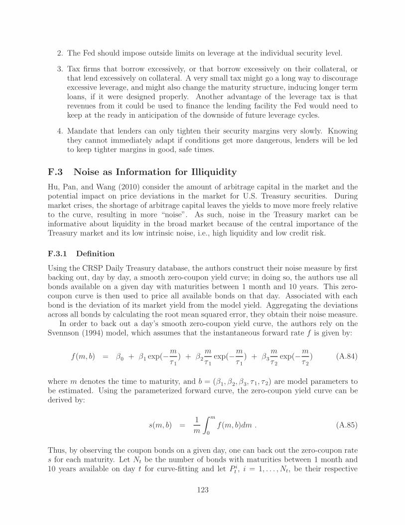
2. The Fed should impose outside limits on leverage at the individual security level.
3. Tax firms that borrow excessively, or that borrow excessively on their collateral, orthat lend excessively on collateral. A very small tax might go a long way to discourageexcessive leverage, and might also change the maturity structure, inducing longer termloans, if it were designed properly. Another advantage of the leverage tax is thatrevenues from it could be used to finance the lending facility the Fed would need tokeep at the ready in anticipation of the downside of future leverage cycles.
4. Mandate that lenders can only tighten their security margins very slowly. Knowingthey cannot immediately adapt if conditions get more dangerous, lenders will be ledto keep tighter margins in good, safe times.
F.3 Noise as Information for Illiquidity
Hu, Pan, and Wang (2010) consider the amount of arbitrage capital in the market and thepotential impact on price deviations in the market for U.S. Treasury securities. Duringmarket crises, the shortage of arbitrage capital leaves the yields to move more freely relativeto the curve, resulting in more “noise”. As such, noise in the Treasury market can beinformative about liquidity in the broad market because of the central importance of theTreasury market and its low intrinsic noise, i.e., high liquidity and low credit risk.
F.3.1 Definition
Using the CRSP Daily Treasury database, the authors construct their noise measure by firstbacking out, day by day, a smooth zero-coupon yield curve; in doing so, the authors use allbonds available on a given day with maturities between 1 month and 10 years. This zero-coupon curve is then used to price all available bonds on that day. Associated with eachbond is the deviation of its market yield from the model yield. Aggregating the deviationsacross all bonds by calculating the root mean squared error, they obtain their noise measure.
In order to back out a day’s smooth zero-coupon yield curve, the authors rely on theSvennson (1994) model, which assumes that the instantaneous forward rate f is given by:
f(m, b) = β0 + β1 exp(−m
τ 1) + β2
m
τ 1exp(−m
τ 1) + β3
m
τ 2exp(−m
τ 2) (A.84)
where m denotes the time to maturity, and b = (β1, β2, β3, τ 1, τ 2) are model parameters tobe estimated. Using the parameterized forward curve, the zero-coupon yield curve can bederived by:
s(m, b) =1
m
∫ m
0
f(m, b)dm . (A.85)
Thus, by observing the coupon bonds on a given day, one can back out the zero-coupon rates for each maturity. Let Nt be the number of bonds with maturities between 1 month and10 years available on day t for curve-fitting and let P i
t , i = 1, . . . , Nt, be their respective
123

market observed prices. The model parameters bt are chosen by minimizing the sum of thesquared deviations between the actual prices and the model-implied prices:
bt = argminbt
Nt∑
i=1
[
P i(bt)− P it
]2(A.86)
where P i(bt) is the model-implied price for bond i on day t given the model parameters bt.Thus, on each day t, the end product of the curve-fitting is the vector of model parametersbt.
In constructing the “noise” measure for a particular day, the authors use all bonds withmaturities between 1 and 10 years available on that day. The “noise” measure does not usebonds with maturities less than 1 year because their information content may be limited dueto the fact that the short end is typically not the object of arbitrage capital; thus, the shortend is used for calibration purposes only.
Let nt denote the number of bonds available on day t, and yit bond i’s observed marketyield. Then, Noiset is defined as:
Noiset =
√
√
√
√
1
nt
nt∑
i=1
[yit − yi(bt)]2 . (A.87)
F.3.2 Inputs and Outputs
• Input: Daily bond prices and yields obtained from the CRSP Daily Treasury databasefrom January 1987 to December 2009.
• Output: The daily liquidity “noise” measure as defined in (A.87).
F.3.3 Empirical Findings
The time series of the liquidity noise measure reveals that during normal times, the noisemeasure is highly persistent and small, meaning that the arbitrage capital on the yieldcurve is effective in keeping the deviations within a range that is unattractive given thetransaction cost. During crises, however, the noise measures spike up, implying a high degreeof misalignment in the yield curve that would have been attractive for relative value tradingduring normal times and are in fact attractive given the contemporaneous transaction cost.Furthermore, the authors find a positive relationship between the noise measure and theon-the-run premium; while the noise measure is, on average, smaller than the on-the-runpremium, it tends to spike up much more significantly during crises. The fact that the noisemeasure spike much more prominently than the on-the-run premiums during liquidity crisesimplies that there is commonality in the pricing errors across the entire yield curve. Andthe heightened commonality during crises is reflected in noisy and misaligned yield curves,which are captured by the noise measure.
The authors also find that factors known to be related to liquidity, such as the VIX, theslope of the yield curve, the Pastor and Stambaugh (2003) liquidity factor, and the RefCorp
124
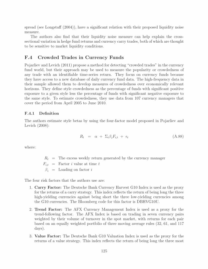
spread (see Longstaff (2004)), have a significant relation with their proposed liquidity noisemeasure.
The authors also find that their liquidity noise measure can help explain the cross-sectional variation in hedge fund returns and currency carry trades, both of which are thoughtto be sensitive to market liquidity conditions.
F.4 Crowded Trades in Currency Funds
Pojarliev and Levich (2011) propose a method for detecting “crowded trades” in the currencyfund world, but their approach may be used to measure the popularity or crowdedness ofany trade with an identifiable time-series return. They focus on currency funds becausethey have access to a new database of daily currency fund data. The high-frequency data intheir sample allowed them to develop measures of crowdedness over economically relevanthorizons. They define style crowdedness as the percentage of funds with significant positiveexposure to a given style less the percentage of funds with significant negative exposure tothe same style. To estimate crowdedness, they use data from 107 currency managers thatcover the period from April 2005 to June 2010.
F.4.1 Definition
The authors estimate style betas by using the four-factor model proposed in Pojarliev andLevich (2008):
Rt = α + ΣiβiFi,t + εt (A.88)
where:
Rt = The excess weekly return generated by the currency manager
Fi,t = Factor i value at time t
βi = Loading on factor i
The four risk factors that the authors use are:
1. Carry Factor: The Deutsche Bank Currency Harvest G10 Index is used as the proxyfor the returns of a carry strategy. This index reflects the return of being long the threehigh-yielding currencies against being short the three low-yielding currencies amongthe G10 currencies. The Bloomberg code for this factor is DBHVG10U.
2. Trend Factor: The AFX Currency Management Index is used as a proxy for thetrend-following factor. The AFX Index is based on trading in seven currency pairsweighted by their volume of turnover in the spot market, with returns for each pairbased on an equally weighted portfolio of three moving average rules (32, 61, and 117days).
3. Value Factor: The Deutsche Bank G10 Valuation Index is used as the proxy for thereturns of a value strategy. This index reflects the return of being long the three most
125

undervalued currencies against being short the three most overvalued currencies amongthe G-10 currencies. The Bloomberg code for this factor is DBPPPUSF.
4. Currency Volatility Factor: The first difference of the (weekly) Deutsche BankCurrency Volatility Index is used as the proxy for foreign exchange volatility. TheBloomberg code for this factor is CVIX.
The authors propose two similar definitions of crowdedness for a given factor:
1. Definition 1: The crowdedness of factor Fi at time t (CFi,t) is defined as the percentageof funds with statistically significant positive exposure to factor Fi less the percentageof funds with statistically significant negative exposure to the same factor:
CFi,t = aFi,t − bFi,t . (A.89)
Here aFi,t is the percentage of funds with statistically significant positive exposure torisk factor Fi over the period t − 25 weeks through t, and bFi,t is the percentage offunds with statistically significant negative exposure to risk factor Fi over the periodt− 25 weeks through t. For both negative and positive exposures, the authors used astandard 95% confidence interval, implying a t-statistic above 1.96 in absolute value.
2. Definition 2: The crowdedness of factor Fi at time t, (C∗Fi,t
) is defined as the per-centage of funds with a βi greater than X less the percentage of funds with a βi lessthan −X , where X is a cutoff chosen by the user:
C∗Fi,t
= a∗Fi,t− b∗Fi,t
(A.90)
where a∗Fi,tis the percentage of funds with βi greater than X over the period t − 25
weeks through t and b∗Fi,tis the percentage of funds with βi less than −X over the
period t− 25 weeks through t.
F.4.2 Inputs and Outputs
• Input: Weekly excess returns for the 107 hedge funds in question from April 2005 toJune 2010.
• Input: Weekly returns for the four factors described in Section F.4.1 from April 2005to June 2010. Specifically, the carry factor is the Deutsche Bank Currency HarvestG10 Index (Bloomber code: DBHVG10U), the trend factor is the AFX CurrencyManagement Index, the value factor is the Deutsche Bank G10 Valuation Index(Bloomberg code DBPPPUSF), and the Currency Volatility Factor is the firstdifference of the weekly Deutsche Bank Currency Volatility Index (Bloomberg code isCVIX).
• Output: Two measures of crowdedness per factor as defined in equations (A.89) and(A.90).
126

F.4.3 Empirical Findings
It is interesting to focus on the authors’ results in 2008. In the first quarter of 2008, a higher-than-usual percentage of funds were significantly exposed to the carry factor and those fundssuffered during the market turbulence in the last quarter of 2008, when carry collapsed.
Similarly, in the first quarter of 2008, a high percentage of funds bet significantly againstvalue. Later in 2008, however, value delivered strong performance, resulting in substantiallosses for the contrarians, who were caught wrong-footed.
The story for trend is different: Trend was a crowded strategy in 2005, but this crowded-ness simply led to flat performance for the trend strategy during this period. After managersgave up on the trend strategy, it delivered strong performance.
Although their sample period was too short for more formal statistical tests, their anal-ysis suggests that there may be an adverse relationship between crowdedness and factorperformance, in particular in the carry and value styles. This phenomenon has also beendocumented in the equity market neutral hedge fund space (see Khandani and Lo (2007,2011)).
F.5 Equity Market Illiquidity
Khandani and Lo (2011) propose two distinct measures of equity market liquidity. Theauthors analyze a contrarian trading strategy which consists of buying losers and sellingwinners. Such a strategy corrects temporary supply-demand imbalances by providing liq-uidity. Although it is a profitable strategy, its profitability has been steadily decreasing sincethe late 1990s, presumably due to the fact that an increasing number of market players havebeen engaging in this liquidity-providing trade thus reducing the liquidity premium of thistrade. A measure of equity market liquidity can be obtained by observing the performanceof such a trading strategy: presumably, when it does very well, there is less liquidity in themarket and vice versa.
The authors’ second measure of market liquidity is related to Kyle’s (1985) “lambda”, inwhich liquidity is measured by a linear regression estimate of the volume required to movethe price of a security by one dollar.
F.5.1 Definition
1. Contrarian Strategy Liquidity Measure: The authors present a simple mean-reversion strategy originally proposed by Lo and MacKinlay (1990a) to proxy for mar-ketmaking (i.e. liquidity provisioning) profits. This high-frequency mean-reversionstrategy is based on buying losers and selling winners over lagged m-minute returns,where m is varied from 5 to 60 minutes. Specifically, a long and a short portfolio areformed at time t by looking at the returns of all stocks in the sample over the previousm minutes. The stocks are sorted into performance deciles, and the strategy is toform a portfolio that is long those stocks in the lowest return-decile over this previousm-minute interval, and short those stocks in the highest return-decile over the previousm-minute interval. This dollar neutral portfolio is then held for q minutes, i.e., untiltime t + q, after which the portfolio formation process is repeated by forming decilesover the returns over the previous m minutes, i.e., the interval from time t+ q −m to
127

t+ q, and then holding these new positions for q minutes, i.e. until time t+2q, and soon.
It should be noted that stocks in both the long and short portfolios are equally weightedand thus the overall portfolio is dollar neutral. Furthermore, no overnight positions areallowed. Finally, the last traded price of a security is used in each m-minute intervalto calculate the returns; hence, the first set of prices for each day are the prices basedon trades just before 9:30am+m minutes and the first set of positions are establishedat 9:30am+2m minutes.
2. Price Impact Liquidity Measure: This approach is motivated by Kyle’s (1985)model in which liquidity is measured by a linear-regression estimate of the volume re-quired to move the price of a security by one dollar. Sometimes referred to as “Kyle’slambda”, this measure is an inverse proxy of liquidity, with higher values of lambdaimplying lower liquidity and market depth. The authors estimate this measure on adaily basis by using all transactions during normal trading hours on each day. Giventhe sequence of intraday returns [Ri,1, Ri,2, . . . , Ri,T ], prices [pi,1, pi,2, . . . , pi,T ], and vol-umes [vi,1, vi,2, . . . , vi,T ] for security i during a specific day, the following regression isestimated:
Ri,t = ci + λi · Sgn(t)log(vi,tpi,t) + εi,t (A.91)
where Sgn(t) ≡ −1 or + 1 depending on the direction of the trade, i.e., “buy” or “sell”,as determined according to the following rule: if Ri,t is positive, the value +1 is assignedto that transaction (to indicate net buying), and if Ri,t is negative, the value −1 isassigned to that transaction (to indicate net selling). Any interval with zero returnreceives the same sign as that of the most recent transaction with a non-zero return(using returns from the prior day, if necessary). The aggregate measure of marketliquidity (MLI) is then given by the daily cross-sectional average of the estimated priceimpact coefficients:
MLI =
∑Ni=1 λi
N(A.92)
where N is the number of stocks for which the measure is calculated on that day.
F.5.2 Inputs and Outputs
• Input: For both measures, the NYSE Trade and Quote (TAQ) data from July 2, 2007to September 28, 2007, are used for all stocks in the S&P 1500. Only the data fromactual trades are used as reported in the “Daily Trades File” of TAQ. Furthermore,only trades that occur during normal trading hours (9:30am to 4:00pm) are used. Theraw data used from TAQ are transaction prices and volumes.
For the “contrarian strategy liquidity measure”, the time t portfolio formation is basedon the returns of the previous m minutes. These returns are calculated by using thelast transaction price in the [t−m, t] interval and comparing it to the last transaction
128

price in the previous interval [t − 2m, t −m]. After the portfolio is formed, it is heldfor q minutes. The authors vary both m and q from 5 to 60 minutes.
For the “price impact liquidity measure”, the returns are calculated on a tick-by-tickbasis.
• Output: The “contrarian strategy liquidity measure” described in Part 1 of SectionF.5.1 and the “price impact liquidity measure” in equations (A.91) and (A.92).
F.5.3 Empirical Findings
The authors find that increases in the price impact liquidity measure were common to allmarket-cap groups and not limited to the smaller stocks. Furthermore, a substantial dropin liquidity in the days leading up to August 6, 2007 was documented. Moreover, thismeasure of liquidity was at its lowest level in the week following the week of August 6.This pattern suggests that some marketmakers, burned by the turn of events in the week ofAugust 6, reduced their marketmaking capital in the following days and in turn caused theprice impacts to substantially rise starting on August 10 and remain high for the followingweek. As quantitative factor portfolios were being deleveraged and unwound during the lasttwo weeks of July 2007, the liquidity premium for the contrarian trading strategy increased,implying higher profits for marketmaking strategies. Indeed, the authors find that during thetwo-week period after the week of August 6, the returns of the contrarian trading strategyare substantially higher than their norm during the whole sample period.
A comprehensive discussion of different theoretical and empirical aspects of liquidity withan overview of the most relevant studies in the area can be found in Amihud (2002) andHasbrouck (2007).
F.6 Serial Correlation and Illiquidity in Hedge Fund Returns
It is a well documented empirical fact that returns to hedge funds and other alternativeinvestments are often highly serially correlated, and Getmansky, Lo, and Makarov (2004)explore several sources of such serial correlation and show that the most likely explanationis illiquidity exposure and smoothed returns. The authors propose an econometric model ofreturn smoothing coefficients; they find that these vary considerably across hedge-fund stylecategories and posit that they may be a useful proxy for quantifying illiquidity exposure.Their argument for why this is the case goes as follows: for illiquid securities, prices are notreadily available and often, linear extrapolation methods of pricing are used, resulting inmore persistent and smoother returns. Even when quotes are obtained from broker/dealers,the phenomenon still exists because broker/dealers also often use linear extrapolation pricingmethods; furthermore, averaging quotes from multiple broker/dealers can lead to smootherprofiles. Thus, hedge funds which invest in more illiquid securities/areas should exhibit ahigher serial correlation in their reported returns.
F.6.1 Definition
The basic model for hedge fund returns presented in the paper differentiates between true re-turns Rt and observed returns Ro
t , i.e., the returns that hedge funds report to their investors.
129

The observed return is a weighted average of the fund’s true returns over time:
Rot = θ0Rt + θ1Rt−1 + · · ·+ θkRt−k , θj ∈ [0, 1] , j = 0, . . . , k
1 = θ0 + θ1 + · · ·+ θk .(A.93)
We call the above model the “smoothing” model. Under the above specification, one canimmediately see that:
E[Rot ] = E[Rt]
Var[Rot ] ≤ Var[Rt]
Corr[Rot , R
ot−m] =
Cov[Rot ,R
ot−m]
Var[Rot ]
=∑k−m
j=0θjθj+m
∑kj=0
θ2j.
(A.94)
Thus, although the observed mean returns are the same as the true mean returns, smoothingresults in a lower observed variance and a higher serial correlation. Funds with θs that aremore “spread out” thus engage in more returns smoothing. The measure which quantifiesthis effect is:
ξ ≡k∑
j=0
θ2j ∈ [0, 1] . (A.95)
The smaller ξ is, the more smoothing is done. Thus, the question becomes how to estimatethe θs. The authors propose two methods of doing this: the maximum likelihood approach(MLE) and the regression approach.
1. MLE approach: Given the specification of the smoothing process in (A.93), the θscan be estimated using maximum likelihood in a fashion similar to the estimationof standard moving-average (MA) time-series models (see Brockwell and Davis (1991,Chapter 8)). Let Xt denote the de-meaned observed return series. The model in (A.93)implies the following properties for Xt:
Xt = θ0ηt + θ1ηt−1 + · · ·+ θkΛt−k
1 = θ0 + θ1 + · · ·+ θk
ηk ∼ N(0, σ2η) .
(A.96)
Denote the given set of realized observations as X = [X1 · · ·XT ]′. Let X = [X1 · · · XT ]
′
where X1 = 0 and Xj = E[Xj|Xj−1, . . . , X1] where j ≥ 2, and define the mean squared
130

error rt of the predicted value of Xt+1 as:
rt =E[(Xt+1 − Xt+1)
2]
σ2η
. (A.97)
Given the above notation, it can be shown that the estimator of the variance is:
σ2η ≡ S(θ) =
∑Tt=1(Xt − Xt)
2
Trt−1. (A.98)
Armed with the above expression, the likelihood function which needs to be maximizedover the parameter space of θs is:
L(θ) = log(S(θ)) + T−1T∑
t=1
log(rt−1) . (A.99)
The function L(θ) is maximized subject to the following constraints:
• Normalization Constraint: θ0 + θ1 + · · ·+ θk = 1.
• Invertibility Constraint: Since the process for XT should be an invertiblemoving-average process, the estimated θs need to satisfy θ1 < (1/2), θ2 < (1 −θ1)/2, etc.
The authors mention that they use the Matlab optimization toolbox in solving theMLE problem. They also mention that they verify the results by running the MA(k)estimation routine in STATA.
2. The regression approach: If one is willing to impose a linear factor model on thetrue returns process of the following form:
Rt = µ + βΛt + εt, E[Λt] = E[εt] = 0, εt,Λt ∼ IID (A.100)
where the true return depends on a common factor Λt, has a mean of µ, and a varianceof σ2, then there is a much simpler method of estimating the θs. By substituting (A.100)into (A.93), the observed returns can be written as a function of lagged factors:
R0t = µ+ β(θ0Λt−1 + · · ·+ θkΛt−k) + ut
= µ+ γ0Λt−1 + · · ·+ γkΛt−k + ut
ut = θ0εt + θ1εt−1 + · · ·+ θkεt−k .
(A.101)
131

By running the above regression, one can estimate the γs and thus the θs:
β = γ0 + γ1 + · · · + γk, θj = γj/β . (A.102)
While the second method for estimating θs is much easier, its downside is that it assumesa specific linear factor structure; specifying the correct factor to use for a given hedge fundentails factor mis-specification risks. Furthermore, even under a reasonable factor, becauseit is an MA process, the ordinary least squares (OLS) estimators will not be efficient andthe usual standard errors are incorrect.
The MLE approach is more general and can yield reliable standard errors at the cost ofbeing more complex and assuming normality of the ηs.
F.6.2 Inputs and Outputs
The authors apply their estimation methods to hedge fund return data using k = 2 lags.
• Input: Monthly hedge fund return data from the TASS database from November1977 to January 2001. They keep only hedge funds that have at least 5 years ofdata history. The authors also run their algorithm on the CSFB/Tremont hedge fundcategory indexes over the same period.
• Input: For the regression case, the appropriate factor Λt for a hedge fund must beselected. The authors use the monthly returns for the S&P 500, although they realizethat this may not be appropriate for some funds.
• Output: The first-, second-, and third-order autocorrelations for each hedge fund’sreturns.
• Output: Each fund’s θs and ξ as defined in (A.95).
F.6.3 Empirical Findings
The authors find that hedge funds that, by common wisdom and self-description, invest inmore illiquid securities, such as Convertible Arbitrage funds, Fixed Income Directional funds,and Emerging Market funds, have higher serial autocorrelations, lower values of ξ, and lowervalues of θ0 compared to funds which typically invest in very liquid securities, such as U.S.Equity funds and Managed Futures funds, whose autocorrelations are near zero and havevalues of θ0 and ξ close to 1.
Furthermore, the authors examine whether phenomena other than the returns smoothingmodel could be causing such high autocorrelations in illiquid funds, such as time varyingexpected returns, time varying leverage, and incentive fee structure; they show that none ofthese can produce the empirically observed high levels of returns persistence.
Finally, although the authors focus on hedge funds, their analysis may be applied toother investments and asset classes, e.g., real estate, venture capital, private equity, art andother collectibles, and other assets for which illiquidity and smoothed returns are even moreproblematic. More generally, their econometric model may be applied to a number of othercontexts in which there is a gap between reported results and economic realities.
132

Further reading on the moving average model presented here can be found in Lo andMacKinlay (1988, 1990a).
F.7 Broader Hedge-Fund-Based Systemic Risk Measures
Chan, Getmansky, Haas, and Lo (2006a, 2006b) consider the broader impact of hedge fundson systemic risk by examining the unique risk/return profiles of hedge funds at both theindividual-fund and aggregate-industry levels and propose three new risk measures for hedgefund investments. The first measure is an autocorrelation-based measure used to proxyhedge fund illiquidity exposures similar to that in Getmansky, Lo, and Makarov (2004) (seeSection F.6 for a summary). The second measure quantifies the probability of liquidation ofa hedge fund, and the third measure is a regime-switching-based model used to quantify thelevel of aggregate distress in the hedge fund sector. The nice feature of the above measuresis that they are indirect measures of risk which require hedge fund returns and sizes as theprimary inputs, making them easy to implement from a data-requirements perspective.
F.7.1 Definition
The three metrics presented in the paper are described below:
1. Autocorrelation-Based Measures: For a given monthly return series of a hedgefund, the first 6 autocorrelation coefficients are estimated. The Q statistic, proposedby Ljung & Box in Ljung and Box (1978) is then calculated according to the formula:
Q = T (T + 2)k∑
j=1
ρ2j/(T − j) . (A.103)
The Q statistic is asymptotically distributed as a χ2k under the null hypothesis of
no autocorrelation. Funds with large positive autocorrelations will exhibit large Qstatistics.
In terms of defining an overall measure of systemic risk (or illiquidity) in the hedgefund sector, the authors propose using a cross-sectional weighted average of hedgefunds’ rolling first-order autocorrelations. Let ρt,i denote hedge fund i’s first-orderautocorrelation in month t using a window of past returns (the authors use 36 months).The aggregate measure of illiquidity ρ∗t is given by:
ρ∗t ≡Nt∑
i=1
ωitρt,i (A.104)
where Nt denotes the number of hedge funds in the sample at time t and ωit denotes
133

the weight of hedge fund i, given by:
ωit ≡ AUMit∑Nt
j=1AUMjt
(A.105)
where AUMjt are the assets under management for fund j at time t.
2. Hedge Fund Liquidation Probability: The authors create a measure of the prob-ability of hedge fund liquidation by running a logit model on a set of factors drivinghedge fund performance. The TASS database of individual hedge fund returns con-tains two subsets: the live database and the graveyard database. Roughly speaking,the graveyard database contains hedge funds which have stopped reporting data toTASS. Thus, a hedge fund that starts out in the live database may end up in thegraveyard database. Hedge funds in the graveyard database are considered to be liq-uidated although this may not necessarily be the case; for a thorough description ofthe TASS database categorizations, see Chan, Getmansky, Haas, and Lo (2006a) orGetmansky, Lo, and Makarov (2004). For tractability, the authors focus on annual ob-servations only, so the dependent variable Zit indicates whether fund i is alive (Zit = 0)or liquidated (Zit = 1) in year t. Thus, for each hedge fund, its time series for Zit willlook like [0, 0, . . . , 0, 1]. Associated with each Zit is a set of explanatory variables listedbelow in Table A.8.
Variable DefinitionAGE Current age of fund in monthsASSETS Log of fund’s AUMASSETS−1 Log of fund’s AUM as of December 31 of previous yearRETURN YTD return for fundRETURN−1 Total returns last yearRETURN−2 Total return two years agoFLOW Fund’s current YTD total dollar inflow
divided by previous year’s AUM, whereinflow in month k is: FLOWk = AUMk −AUMk−1(1 +Rk)where Rk is month k’s return
FLOW−1 Last year’s inflow over AUM the year beforeFLOW−2 Inflow 2 years ago over AUM 3 years ago
Table A.8: Explanatory Variables Used In Estimating Liquidation Probabilities
Therefore, the logit model to be estimated is:
Zit = G
(
β0 + β1AGEit + β2ASSETSit−1 +
β3RETURNit + β4RETURNit−1 + β5RETURNit−2 +
β6FLOWit + β7FLOWit−1 + β8FLOWit−2 + εit
)
.
(A.106)
134

The above model is estimated via the standard maximum likelihood method for logitmodels (see, for example, Woolridge (2002)). After the betas have been estimated, onecan estimate the probability of liquidation for a hedge fund at time t as:
pit =exp(X
′
itβ)
1 + exp(X′
itβ). (A.107)
The indicator of systemic risk across the hedge fund industry is the mean and/ormedian of each fund’s pit.
3. Regime-Switching-Based Systemic Risk Measure: The authors use a two stateregime-switching model. Denote by Rt the return of a hedge fund index in period tand suppose it satisfies the following:
Rt = Iit · R1t + (1− It) · R2t , Rit ∼ N (ui, σ2i ) (A.108)
It =
1 with probability p11 if It−1 = 1
1 with probability p21 if It−1 = 0
0 with probability p12 if It−1 = 1
0 with probability p22 if It−1 = 0
(A.109)
The transition probabilities pij , along with the means and variances of R1t and R2t,are estimated via maximum likelihood of the above model. Note that the specificationof the process It is a Markov Chain. Because the k-step transition matrix of a Markovchain is simply given by Pk, the conditional probability of the regime It+k given thereturns up to time t is:
Prob(It+k = 1|Rt) = π1 + (p11 − p21)k[Prob(It = 1|Rt)− π1] (A.110)
π1 ≡ p21p12 + p21
(A.111)
where Prob(It = 1|Rt) is the probability that the date t regime is 1 given the historicaldata up to and including date t. Using similar recursions of the Markov chain, theconditional expectation of Rt+k is:
E[Rt+k|Rt] = a′tPkµ
at = [Prob(It = 1|Rt) Prob(It = 2|Rt)]′
µ ≡ [µ1 µ2]′ .
(A.112)
Thus, once the above model is estimated, the hedge fund systemic risk indicator (HF-SRI) for the overall hedge fund industry is calculated as the sum of the probabilities
135

of being in the low-mean state at time t for each hedge fund index:
HFSRIt =n∑
i=1
Prob(I it = low-mean state of i|Rit) (A.113)
where n denotes the number of hedge fund indexes. Note that the summed probabili-ties, even if renormalized to lie in the unit interval, cannot be interpreted formally asa probability because the regime-switching process was specified individually for eachindex, not jointly across all indexes. Therefore, the interpretation of the low-meanstate for convertible arbitrage may be quite different than the interpretation of thelow-mean state for equity market neutral. Nevertheless, as an aggregate measure ofthe state of the hedge fund industry, the summed probabilities may contain usefulinformation about systemic risk exposures.
F.7.2 Inputs and Outputs
Below, we categorize the inputs and outputs needed for each of the 3 systemic risk measurespresented.
1. Autocorrelation-Based Measures:
• Input: Monthly hedge fund return data and AUM for all funds in the TASSdatabase with at least 36 consecutive months of non-missing returns, along withthe number of funds each month (at the bottom, measured by the right verticalaxis), from January 1977 to August 2004.
• Ouput: For each hedge fund, its Q statistic defined in (A.103).
• Output: The systemic liquidity indicator ρ∗t defined in (A.104).
2. Hedge Fund Liquidation Probability:
• Input: Using all funds in both the live and graveyard databases of the TASSdatabase for which there are at least 2 years of history, collect the data in TableA.8 from January 1994 to August 2004.
• Ouput: The probability of liquidation for each hedge fund pit as defined inequation (A.107).
3. Regime-Switching-Based Systemic Risk Measure:
• Input: The monthly returns of each of the 14 CSFB/Tremont hedge fund indexesfrom January 1994 to August 2004.
• Output: The hedge fund systemic risk indicator HSFRI at time t as defined in(A.113).
• Output: Predictions about the expected return of the index as well as the prob-ability of being in each state at time (t + k) (equations (A.112) and (A.110)respectively).
136

F.7.3 Empirical Findings
The authors find that the hedge fund liquidity indicator ρ∗t shows considerable swings overtime, with dynamics that seem to be related to liquidity events. Furthermore, over the latterperiod of their sample (2001–2004), this indicator is on the rise, implying that hedge fundsare taking on more illiquidity exposure.
In terms of the hedge fund liquidation probabilities, they find that the average liquidationprobability for funds in 2004 (end of their sample) is over 11%, higher than the historicalunconditional attrition rate of 8.8%. A higher attrition rate is not surprising for a rapidlygrowing industry, but it may foreshadow potential instabilities that can be triggered byseemingly innocuous market events.
When running the regime-switching model on the various hedge fund categories, it isinteresting to note that the two state pairings are not always (high mean, low volatility)and (low mean, high volatility). In fact, for equity market neutral, global macro, andlong/short equity, the pairings are the opposite, indicating that these strategies performwell in high volatility states. HFSRI has local maxima in 1994 and 1998 as expected, butthere is a stronger peak around 2002, largely due to equity market neutral, global macro, andlong/short equity funds. This pattern corresponds remarkably well to the common wisdomthat, over that period, these three strategies underperformed. In 2004, the probability ofbeing in the low-mean state is high for a number of hedge fund indexes, foreshadowingincreased leverage and ultimately increased systemic risk.
G Matlab Program Headers
In this section, we provide a listing of the headers for all the Matlab programs availableto compute the risk analytics described in this survey. The complete sourcecode for theseprograms is available at http://.
G.1 Function delta co var
function dcovar = delta_co_var(output_returns, input_returns,
lagged_factors_returns, quantile)
%
% Based on the paper "CoVar", Tobias Adrian and Markus K. Brunnermeier.
% Calculates the delta_covar of an output institution (or the system) on
% another institution.
%
% PARAMETERS:
% output_returns - The returns of the output institution or system.
% An (nx1)-vector.
% input_returns - The returns of the input institution whose contribution
% we want to quantify. An (nx1)-vector.
% lagged_factors_returns - The lagged returns (lag = 1) for the factors as
% used in eq. 6 of the paper. An ((n+1)xk)-matrix.
% quantile - The quantile we want to use (0.05 or 0.01) in the paper.
137

G.2 Function quantile regression
function betas = quantile_regression(y,X,q)
%
% Calculates the q-quantile regression coefficients.
%
% PARAMETERS:
% y - The response variable. An (nx1)-vector.
% X - the matrix of regressors An (nxk)-vector.
% q - the quantile i.e. 0.5 for median regression.
G.3 Function co risk
function c = co_risk(output_cds_spreads,input_cds_spreads,
risk_factors_series,q,risk_factors_values )
%
% Calculates the conditional co-risk between two institutions.
%
% PARAMETERS:
% output_cds_spreads - The cds-spreads time series for the output
% institution. An (nx1)-vector.
% input_cds_spreads - The cds-spreads time series for the input institution.
% An (nx1)-vector.
% risk_factors_series - Risk-factors time series. An (nxk)-matrix.
% q - The quantile. The paper uses q = 0.95.
% risk_factors_values - the values of the risk factors at the period we
% calculate the co-risk. A (1xk)-vector.
G.4 Function turbulence
function [turbulence_series, threshold, turbulent_periods] =
turbulence(asset_returns,q)
%
% Calculates the turbulence of each period, the q-percentile of turbulence
% distribution and the turbulent periods.
%
% PARAMETERS:
% asset_returns - A matrix of asset returns. Rows are different dates.
% Columns are different assets.
% q - The percentile. In the paper q = 0.75.
%
% OUTPUTS:
% turbulence_series - The turbulence for each period in the sample.
% threshold - The q-percentile of turbulence distribution.
% turbulent_periods - The periods where turbulence > quantile.
138
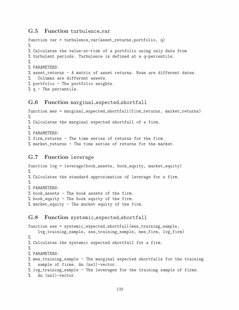
G.5 Function turbulence var
function var = turbulence_var(asset_returns,portfolio, q)
%
% Calculates the value-at-risk of a portfolio using only data from
% turbulent periods. Turbulence is defined at a q-percentile.
%
% PARAMETERS:
% asset_returns - A matrix of asset returns. Rows are different dates.
% Columns are different assets.
% portfolio - The portfolio weights.
% q - The percentile.
G.6 Function marginal expected shortfall
function mes = marginal_expected_shortfall(firm_returns, market_returns)
%
% Calculates the marginal expected shortfall of a firm.
%
% PARAMETERS:
% firm_returns - The time series of returns for the firm.
% market_returns - The time series of returns for the market.
G.7 Function leverage
function lvg = leverage(book_assets, book_equity, market_equity)
%
% Calculates the standard approximation of leverage for a firm.
%
% PARAMETERS:
% book_assets - The book assets of the firm.
% book_equity - The book equity of the firm.
% market_equity - The market equity of the firm.
G.8 Function systemic expected shortfall
function ses = systemic_expected_shortfall(mes_training_sample,
lvg_training_sample, ses_training_sample, mes_firm, lvg_firm)
%
% Calculates the systemic expected shortfall for a firm.
%
% PARAMETERS:
% mes_training_sample - The marginal expected shortfalls for the training
% sample of firms. An (nx1)-vector.
% lvg_training_sample - The leverages for the training sample of firms.
% An (nx1)-vector.
139

% ses_training_sample - The systemic expected shortfalls for the training
% sample of firms. An (nx1)-vector.
% mes_firm - The marginal expected shortfall for the firm.
% lvg_firm - The leverage for the firm.
G.9 Function contrarian trading strategy
function ret = contrarian_trading_strategy(input_returns, realized_returns)
%
% Calculates the cumulative return of the contrarian trading strategy.
%
% PARAMETERS:
% input_returns - The returns of the securities used to calculate the weights
% of the strategy. Rows are the different periods. Columns are the
% different securities.
% realized_returns - The realized returns of the securities to calculate
% the performance of the strategy. Rows are the different periods.
% Columns are the different securities.
G.10 Function kyles lambda
function mli = kyles_lambda(returns, prices, volumes)
%
% Calculates Kyle’s lambda (price impact liquidity measure).
%
% PARAMETERS:
% returns - The returns of different securities. Rows are different dates
% and columns are different securities.
% prices - The closing prices of the securities. Rows are different dates
% and columns are different securities.
% voumes - The trading volumes of the securities. Rows are different dates
% and columns are different securities.
G.11 Function systemic liquidity indicator
function [q_stats sys_liquidity_ind] =
systemic_liquidity_indicator(funds_returns,assets_under_management)
%
% Calculates the Q-stats for each fund and the systemic liquidity indicator.
%
% PARAMETERS:
% funds_returns - The monthly returns of the funds. A (nxk)-matrix. Rows
% are the different periods. Columns are the different funds.
% assets_under_management - The assets under management for the different
% funds. A (kx1)-vector.
%
140

% OUTPUTS:
% q_stats - The q-statistics for the different funds’ returns.
% A (kx1)-vector.
% sys_liquidity_ind - The systemic liquidity indicator.
G.12 Function probability liquidation model
function coeffs = probability_liquidation_model(aums, returns, flows,
is_liquidated_series)
%
% Calculates the coefficients in the logit model for probability of
% liquidation of a fund.
%
% PARAMETERS:
% aums - The series of AUMS for the different funds. An (nxk)-matrix. Rows
% are the different months. Columns are the different funds.
% returns - The series of returns for the different funds. An (nxk)-matrix.
% Rows are the different months. Columns are the different funds.
% flows - The series of flows for the different funds. A (nxk)-matrix. Rows
% are the different months. Columns are the different funds.
% is_liquidated_series - A binary (nxk)-matrix . If the (i,j) component = 1
% it denotes that fund j is liquidated at period i.
G.13 Function crowded trades
function crowdedness = crowded_trades(funds_returns, factor_returns,
factor_index, threshold)
%
% Calculates the crowdedness series of a factor.
%
% PARAMETERS:
% funds_returns - A matrix of funds returns. Rows are different dates.
% Columns are different assets.
% factor returns - A matrix of funds returns. Rows are different dates.
% Columns are different assets. For the paper there are 4 factors,
% i.e., 4 cols.
% factor_index - The factor whose crowdedness we want to calculate
% threshold. If it is specified then crowdedness is found with
% respect to beta greater than threshold.
G.14 Function cca
function [put_price systemic_risk_indicator_contribution] = cca(equity,
volatility,risk_free_rate,default_barrier,time_to_maturity,cds_spread)
%
% Based on the paper "Systemic CCA - A Model Approach to Systemic Risk" by
141

% D. F. Gray, A.A. Jobst.
% Calculates the price of the put option and the contribution of the
% company to the systemic risk indicator suggested in the paper.
%
% PARAMETERS:
% equity - The market value of the equity of the company.
% volatility - The volatility of the equity.
% risk_free_rate - The risk free rate.
% default_barrier - Face value of the outstanding debt at maturity.
% time_to_maturity - Time to maturity of the debt.
% cds_spread - The cds spread.
%
% OUTPUTS:
% put_price - The price of the put
% systemic_risk_indicator_contribution - The contribution of this firm to
% the systemic risk indicator
G.15 Function distressed insurance premium
function dip = distressed_insurance_premium(default_probabilities,
correlations)
%
% Calculates the distressed insurance premium.
%
% PARAMETERS:
% default_probabilities - The default probabilities of the banks.
% An (nx1)-vector.
% correlations - The correlation matrix of the assets’ returns of the banks.
G.16 Function credit funding shock
function [capital_losses defaulted_banks] =
credit_funding_shock(default_bank,
capitals, interbank_loans, lambda, rho, delta)
%
% Simulates a credit and funding shock in the banking system.
%
% PARAMETERS:
% default_bank - The bank that is initially triggered to default. An integer
% 1<=default_bank <=n.
% capitals - The capitals of the banks. An (nx1)-vector. A bank defaults if
% its capital becomes negative.
% interbank_loans - An (nxn)-matrix describing the loans between banks. The
% (i,j)-component denotes a loan from bank j to bank i.
% lambda - The loss given default parameter. In the paper it is set to 1.
% rho - The loss of funding fraction. In the paper it is set to 0.35.
142

% delta - The loss parameter due to forced selling. In the paper it is set
% to 1.
%
% OUTPUTS:
% capital_losses - The capital losses of the banks.
% defaulted_banks - The banks that default. An (nx1)-binary vector where 1
% denotes default.
G.17 Function pca
function [Sigma, eigenvalues, eigenvectors] = pca(asset_returns)
%
% Calculates the covariance matrix of
% the returns for different assets and its eigenvalues and eigenvectors.
%
% PARAMETERS:
% asset_returns - The time series of asset returns. An (nxk)-matrix. Rows
% are the different dates. Columns are the different assets.
%
% OUTPUTS:
% Sigma - The covariance matrix of the asset returns.
% eigenvalues - The eigenvalues of the covariance matrix.
% eigenvectors - A matrix with the corresponding eigenvectors of the
% covariance matrix as its columns.
G.18 Function linear granger causality
function p_value = linear_granger_causality(input_institution_returns,
output_institution_returns)
%
% Calculates the p-value of the linear Granger-causal relationship between
% input_institution_returns and output_institution_returns.
%
% PARAMETERS:
% input_institution_returns - The time series returns of the input
% institution. An (nx1)-vector.
% output_institution_returns - The time series returns of the output
% institution. An (nx1)-vector.
G.19 Function hac regression
function [betas, V_hat] = hac_regression(y,X,
truncation_lag_to_observations_ratio)
%
% Calculates the regression coefficients and the HAC ("heteroskedasticity
% and autocorrelation consistent") estimator.
143

%
% PARAMETERS:
% y - The dependent variable An (nx1)-vector.
% X - The covariates. An (nxk)-vector.
% truncation_lag_to_observations_ratio - The truncation lag to number of
% observations ratio used to construct the HAC estimator.
%
% OUTPUTS:
% betas - The regression coefficients. A (kx1)-vector.
% V_hat - The HAC estimator.
G.20 Function dynamic causality index
function [connection_matrix_robust, connection_matrix, dci] =
dynamic_causality_index(asset_returns,statistical_significance_threshold)
%
% Based on the paper "Econometric Measures of Systemic Risk in the Finance
% and Insurance Sectors" by M. Billio, M. Getmansky, A.W. Lo, L. Pelizzon
% Calculates the dynamic causality index and the adjacency matrix of linear
% Granger causal relationships for different institutions based on their
% returns.
%
% PARAMETERS:
% asset_returns - The time series of institutions returns. An (nxk)-matrix
% Rows are the different dates. Columns are the different institutions.
% statistical_significance_threshold - The threshold for p-value that
% determines if the linear Granger-causal relationship is statistically
% significant. Usually 0.05 or 0.01.
%
% OUTPUTS:
% connection_matrix_robust - The adjacency matrix describing the linear
% Granger-causal relationships among the institutions. If
% connection_matrix(i,j) = 1 then institution i affects institution j.
% It corrects for autocorrelations and heteroskedasticity.
% connection_matrix - The adjacency matrix describing the linear Granger-
% causal relationships among the institutions. If
% connection_matrix(i,j) = 1 then institution i affects institution j.
% It does not correct for autocorrelations and heteroskedasticity.
% dci - The dynamic causality index for the robust matrix.
G.21 Function dijkstra
function distances = dijkstra(A,node)
%
% Implements the Dijkstra algorithm; returns the shortest path lengths
% between the initial and all other nodes.
144

%
% PARAMETERS:
% A - The (nxn) adjacency matrix.
% node - The initial node from which we calculate all the shortest paths to
% any other node.
G.22 Function calc closeness
function cl = calc_closeness(adjacency_matrix, node)
%
% Calculates the closeness of a node in a network.
%
% PARAMETERS:
% adjaceny_matrix - The adjacency matrix of the network.
% node - The node.
G.23 Function network measures
function [in_connections, out_connections, in_out_connections, in_from_other,
out_to_other, in_out_other, closeness, eigenvector_centrality]=
network_measures(adjacency_matrix, groups)
%
% For all the nodes of the network it calculates a few network measures
%
% PARAMETERS:
% adjacency_matrix - The adjacency matrix describing the network.
% An (nxn)-matrix.
% groups - A vector describing the different categories of nodes. i.e. if
% group = [2 6] that means that we have 3 groups of nodes. Group 1
% nodes 1,2, Group 2 nodes 3,4,5,6 Group 3 nodes 7 until n.
%
% OUTPUTS:
% in_connections - For each node the number of incoming links.
% out_connections - For each node the number of outcoming links.
% in_out_connections - For each node the sum of incoming and outcoming links.
% in_from_other - For each node the number of incoming links from nodes in
% different categories.
% out_to_other - For each node the number of outcoming links to nodes in
% different categories.
% in_out_other - For each node the sum of in_from_other and out_to_other.
% closeness - For each node the average shortest path lengths to reachable
% nodes.
% eigenvector_centrality - For each node its eigenvector centrality.
145

G.24 Function absorption ratio
function ar = absorption_ratio(asset_returns, fraction_eigenvectors)
%
% Calculates the absorption ratio for a time series of asset returns
%
% PARAMETERS:
% asset_returns - A matrix of asset returns. Rows are different dates.
% Columns are different assets. In the paper number of rows = 500.
% fraction_eigenvectors - The fraction of eigenvectors used to calculate the
% absorption ratio. In the paper it is 0.2.
G.25 Function dar
function ar_shift = dar(absorption_ratios, fraction)
%
% Calculates the standardized AR shift
%
% PARAMETERS:
% absorption_ratios - A vector of absorption ratios. In the paper
% absorption ratios are given for 1 year.
% fraction - Number of days in the short term absorption ratio over number
% of days in the long term absorption ratio. In the paper 15/252 if we
% consider a year having 252 absorption ratios.
G.26 Function undirected banking linkages
function undirected = undirected_banking_linkages(bank_claims,
non_bank_claims, non_bank_liabilities)
%
% Calculates the undirected network of banking linkages for n
% countries.
%
% PARAMETERS:
% bank_claims - An (nxn)-matrix. Its (i,j) component shows the bank claims
% from country i to banks in country j.
% non_bank_claims - An (nxn)-matrix. Its (i,j) component shows the claims
% from banks in country i to non-banks in country j.
% non_bank_liabilities - An (nxn)-matrix. Its (i,j) component shows the
% liabilities of banks in i to non-banks in j.
G.27 Function directed banking linkages
function directed = directed_banking_linkages(initial_net_bank_claims,
initial_net_non_bank_claims, final_net_bank_claims,
final_net_non_bank_claims)
146

%
% Calculates the diretced network of banking linkages for n
% countries between two time instants t1 and t2.
%
% PARAMETERS:
% initial_net_bank_claims - An (nxn)-matrix. Its (i,j) component shows the
% net bank claims from country i to banks in country j at t1. Antisymmetric
% matrix.
% initial_net_non_bank_claims - An (nxn)-matrix. Its (i,j) component shows
% the net claims from banks in country i to non-banks in country j at t1.
% final_net_bank_claims - An (nxn)-matrix. Its (i,j) component shows the
% net bank claims from country i to banks in country j at t2. Antisymmetric
% matrix.
% final_net_non_bank_claims - An (nxn)-matrix. Its (i,j) component shows the
% net claims from banks in country i to non-banks in country j at t2.
G.28 Function optimal gap thresholds
function [nts_thresholds, true_positive_thresholds] =
optimal_gap_thresholds(indicators_series, is_crisis_series,horizon,
max_thresholds)
%
% Based on the paper "Towards an operational framework for financial
% stability:"fuzzy" measurement and its consequences by C. Borio, M.
% Drehmann.
%
% Calculates the optimal gap thresholds according to nts ratio and
% true positive rate.
%
% PARAMETERS:
% indicators_series - The joint signal indicators yearly time series.
% An (nx2)-matrix.
% is_crisis_series - A binary nx1 vector. 1 signals that there is a crisis
% horizon. In the paper it is set 1 to 3 years.
% max_thresholds - A (2x1)-vector with the maximum thresholds for the two
% indicators. They are integer values.
%
% OUTPUTS
% nts_thresholds - The optimal thresholds for the two indicators when the
% objective function is nts. A (2x1)-vector.
% true_positive_thresholds - The optimal thresholds for the two indicators
% when the objective function is true_positive rate. A (2x1)-vector.
G.29 Function joint gap indicators
function [nts num_predicted_crises] =
147

joint_gap_indicators(indicators_series, thresholds, is_crisis_series,
horizon)
%
% Calculates the signal to noise ratio and the number of predicted crises
% of joint signal indicators for particular thresholds
%
% PARAMETERS:
% indicators_series - The joint signal indicators yearly time series.
% An (nx2)-matrix.
% thresholds - The thresholds used to signal a crisis. A (2x1)-vector.
% is_crisis_series - A binary (nx1)-vector. 1 signals that there is a
% crisis.
% horizon - In the paper it is set 1 to 3 years.
G.30 Function stress scenario selection
function forecast_error = stress_scenario_selection(gdp_growth_series)
%
% Based on paper: "Macro Stress Tests and Crises: What can we learn? R.
% Alfaro, M. Drehman, 2009.
% Calculates the worst forecast error in an AR process which is
% subsequently used as a stress scenario.
%
% PARAMETERS:
% gdp_growth_series - The gdp growth series as an (nx1)-vector.
G.31 Function fit ar model
function [regressor_coefficients, order] = fit_ar_model(y_series, max_order)
%
% Fits an AR model to the y_series. It selects the order that is less than
% max_order and minimizes the BIC.
%
% PARAMETERS:
% y_series - An (nx1)-vector that we ’ll fit an AR model to.
% max_order - The maximum order of AR model we will try.
G.32 Function systemic risk exposures
function res = systemic_risk_exposures(exposures,k)
%
% This is based on the paper "Systemic Risk Exposures: A 10-by-10-by-10
% approach" by D.Duffie.
% For each stress test, for each important institution it gives the
% k companies that the important institution has largest exposures on.
%
148

% PARAMETERS:
% exposures - The exposures of the important institutions under different
% stress tests (gains or losses). An (nxpxm)-array. There are m stress
% tests and n important institutions. For each test for each important
% institution there are exposures to p companies.
Classification of Models
The research literature on the measurement of systemic financial risk is large and growingrapidly. Like the problem it addresses, the set of approaches adopted is wide-ranging andcomplex. To fully comprehend such a diverse ecosystem, a taxonomy of the various tech-niques is often useful. This article, for example, is organized primarily around the datarequirements of the various approaches. However, the following is another possible catego-rization, which focuses, instead, on the systemic features examined and the methods used:
• Illiquidity measures i – models focusing on effective supply and demand for secu-rities, mostly in the over-the-counter markets, and typically applying regression tech-niques.
• Probability-distribution measures p – these apply a more traditional risk-management approach, which assumes that risk is driven by a stable and exogenousdata-generating process.
• Contingent-claim and default measures c – models with a salient focus on asym-metric and/or nonlinear payoffs, including the asymmetries arising from the limited-liability structure of financial firms.
• Network analysis measures n – these concentrate attention on the relationships(typically contractual) between participants in the system, and frequently apply graph-theoretic techniques.
• Macroeconomic measures m – models focusing on high-level features of the fi-nancial system and/or macro economy, and typically applying time-series techniques,including forecasting.
The tags given here in guillemets also appear in the list of references below to indicate theapproach taken by the individual research works. There remains here a large residual cate-gory of other measures, denoted by the tag o, as any such categorization is necessarilyapproximate and incomplete. No single classification scheme will be appropriate for all pur-poses.
149
References
Abbe, E., A. Khandani, and A. W. Lo, 2011, “Privacy-Preserving Methods for SharingFinancial Risk Exposures,” working paper, MIT Laboratory for Financial Engineering.
Acharya, V., L. Pedersen, T. Philippon, and M. Richardson, 2010, “Measuring SystemicRisk,” working paper, New York University.
Acharya, V., and M. Richardson (eds.), 2009, Restoring Financial Stability: How to Repaira Failed System. Wiley, New York.
Adalid, R., and C. Detken, 2007, “Liquidity Shocks and Asset Price Boom/Bust Cycles,”ECB Working Paper 732, European Central Bank.
Adrian, T., and M. Brunnermeier, 2010, “CoVaR,” Staff Report 348, Federal Reserve Bankof New York.
Adrian, T., and H. S. Shin, 2009, “The shadow banking system: implications for financialregulation,” Financial Stability Review, 19, 1–10.
, 2010, “Liquidity and leverage,” Journal of Financial Intermediation, 19(3), 418–437.
Aikman, D., P. Alessandri, B. Eklund, P. Gai, S. Kapadia, E. Martin, N. Mora, G. Sterne,and M. Willison, 2010, “Funding Liquidity Risk in a Quantitative Model of SystemicStability,” in Financial Stability, Monetary Policy, and Central Banking, ed. by R. A.Alfaro. Central Bank of Chile, 12th Annual Conference of the Central Bank of Chile,November 6-7, 2008.
Alessi, L., and C. Detken, 2009, “Real time early warning indicators for costly asset priceboom/bust cycles: A role for global liquidity,” ECB Working Paper 1039, European Cen-tral Bank.
Alexander, L., 2010, “Opening Remarks,” working paper, Measuring Systemic Risk: AConference Sponsored by the Milton Friedman Institute, the Chicago Fed, and the NewYork Fed.
Alfaro, R., and M. Drehmann, 2009, “Macro stress tests and crises: what can we learn?,”BIS Quarterly Review, pp. 29–41.
Allen, F., and D. Gale, 2000, “Financial Contagion,” Journal of Political Economy, 108(1),1–33.
Amihud, Y., 2002, “Illiquidity and stock returns: Cross-section and time-series effects,”Journal of Financial Markets, 5, 31–56.
Ang, A., and G. Bekaert, 2002, “International asset allocation with regime shifts,” Reviewof Financial Studies, 15(4), 1137–1187.
Ang, A., and J. Chen, 2002, “Asymmetric correlations of equity portfolios,” Journal ofFinancial Economics, 63(3), 443–494.
150

Aragon, G., and P. Strahan, 2009, “Hedge funds as liquidity providers: Evidence from theLehman bankruptcy,” NBER Working Paper Series 15336, National Bureau of EconomicResearch.
Ashcraft, A., and T. Schuermann, 2008, “Understanding the Securitization of SubprimeMortgage Credit,” Federal Reserve Bank of New York Staff Reports 318, Federal ReserveBank of New York.
Axelrod, R., 1997, The Complexity of Cooperation: Agent-Based Models of Competition andCollaboration. Princeton University Press, Princeton, NJ.
Bank of England, B., 2009, “The Role of Macroprudential Policy,” Discussion paper, Bankof England.
Basel Committee on Banking Supervision, 2010, “Countercyclical capital buffer proposal,”Consultative document, Bank for International Settlements.
, 2011, “Global systemically important banks: Assessment methodology and theadditional loss absorbency requirement,” Consultative document, Bank for InternationalSettlements.
Basurto, M., and P. Padilla, 2006, “Portfolio Credit Risk and Macroeconomic Shocks: Ap-plications to Stress Testing Under Data-Restricted Environments,” IMF Working PaperWP/06/283, IMF.
Benston, G. J., and G. G. Kaufman, 1997, “FDICIA After Five Years,” The Journal ofEconomic Perspectives, 11(3), 139–158.
Bignon, V., M. Flandreau, and S. Ugolini, 2009, “Bagehot for beginners: The making oflending of last resort operations in the mid-19th century,” Norges Bank working paper2009/22, Norges Bank.
Billio, M., and S. Di Sanzo, 2006, “Granger-causality in Markov switching models,” Dept.of Economics Research Paper Series 20WP, University Ca’ Foscari of Venice.
Billio, M., M. Getmansky, A. W. Lo, and L. Pelizzon, 2010, “Econometric measures ofsystemic risk in the finance and insurance sectors,” NBER Working Paper 16223, NBER.
Black, F., and M. Scholes, 1973, “The pricing of options and corporate liabilities,” Journalof Political Economy, 81(3), 637–654.
Bollerslev, T., 1986, “Generalized autoregressive conditional heteroskedasticity,” Journal ofEconometrics, 31(3), 307–327.
Boot, A., and A. Thakor, 1993, “Self-Interested Bank Regulation,” American EconomicReview, 83(2), 206–212.
Bordo, M., 1990, “The Lender of Last Resort: Alternative Views and Historical Experience,”Federal Reserve Bank of Richmond Economic Review, 1990, 18–29.
151

Borio, C., 2009, “The macroprudential approach to regulation and supervision,” workingpaper, VoxEU.org, 14 April 2009.
, 2010, “Implementing a macroprudential framework: blending boldness and realism,”working paper, Bank for International Settlements, Keynote address for the BIS-HKMAresearch conference, Honk Kong SAR, 5-6 July 2010.
Borio, C., and M. Drehmann, 2008, “Towards an operational framework for financial stabil-ity: “Fuzzy” measurement and its consequences,” 12th Annual Conference of Banco deChile on Financial Stability, Monetary Policy and Central Banking.
Borio, C., and M. Drehmann, 2009a, “Assessing the risk of banking crises – revisited,” BISQuarterly Review, 2009(2), 29–46.
, 2009b, “Towards an operational framework for financial stability: ’fuzzy’ measure-ment and its consequences,” BIS Working Papers 284, Bank for International Settlements.
Borio, C., and P. Lowe, 2004, “Securing sustainable price stability: should credit come backfrom the wilderness?,” BIS Working Paper 157, Bank for International Settlements.
Bossaerts, P., 2009, “What Decision Neuroscience Teaches Us About Financial DecisionMaking,” Annual Review of Financial Economics, 1, 383–404.
Bottega, J. A., and L. F. Powell, 2010, “Creating a Linchpin for Financial Data: The Needfor a Legal Entity Identifier,” working paper, Board of Governors of the Federal Reserve.
Bouchaud, J., J. D. Farmer, and F. Lillo, 2009, “How Markets Slowly Digest Changes inSupply and Demand,” in Handbook of Financial Markets: Dynamics and Evolution, ed.by H. Thorsten, and K. chenk Hoppe. Elsevier, New York.
Boyd, J., and M. Gertler, 1994, “Are Banks Dead? Or Are the Reports Greatly Exagger-ated?,” Federal Reserve Bank of Minneapolis Quarterly Review, 18(3), 2–23.
Boyson, N. M., C. W. Stahel, and R. M. Stulz, 2010, “Hedge Fund Contagion and LiquidityShocks,” Journal of Finance, 65(5), 1789–1816.
Breiman, L., J. Friedman, R. Olshen, and C. Stone, 1984, Classification and RegressionTrees. Wadsworth and Brooks Cole Advanced Books and Software, Pacific Grove, CA.
Breuer, T., M. Jandacka, K. Rheinberger, and M. Summer, 2009, “How to Find Plausible,Severe and Useful Stress Scenarios,” International Journal of Central Banking, 5(3), 205–224, Bank for International Settlements.
Brockwell, P., and R. Davis, 1991, Time Series: Theory and Methods. Springer, New York,NY.
Brown, C. O., and I. S. Din, 2011, “Too Many to Fail? Evidence of Regulatory ForbearanceWhen the Banking Sector Is Weak,” Review of Financial Studies, 24(4), 1378–1405.
Brunnermeier, M., and L. Pedersen, 2009, “Market liquidity and funding liquidity,” Reviewof Financial Studies, 22(6), 2201–2238.
152

Brunnermeier, M. K., A. Crockett, C. A. Goodhart, A. D. Persaud, and H. S. Shin, 2009,“The Fundamental Principles of Financial Regulation,” Geneva Reports on the WorldEconomy 11, International Center for Monetary and Banking Studies.
Brunnermeier, M. K., G. Gorton, and A. Krishnamurthy, 2010, “Risk Topography,” workingpaper, Princeton University.
Caballero, R. J., 2009, “The ’Other’ Imbalance and the Financial Crisis,” MIT Departmentof Economics Working Paper No. 09-32, Massachusetts Institute of Technology.
Capuano, C., 2008, “The option-iPoD. The Probability of Default Implied by Option PricesBased on Entropy,” IMF Working Paper 08/194, International Monetary Fund.
Caruana, J., 2010a, “Financial Stability: Ten Questions and about Seven Answers,” inReserve Bank of Australia 50th Anniversary Symposium.
, 2010b, “Macroprudential policy: could it have been different this time?,” workingpaper, Bank for International Settlements, Peoples Bank of China seminar on macropru-dential policy in cooperation with the International Monetary Fund: Shanghai, Monday18 October 2010.
Chan, N., M. Getmansky, S. M. Haas, and A. W. Lo, 2006a, “Do Hedge Funds IncreaseSystemic Risk?,” Federal Reserve Bank of Atlanta Economic Review, 91(4), 49–80.
, 2006b, “Systemic risk and hedge funds,” in The Risks of Financial Institutions, ed.by M. Carey, and R. Stulz. University of Chicago Press, Chicago, IL, pp. 235–330.
Chan-Lau, J., 2009, “Co-risk measures to assess systemic financial linkages,” Imf workingpaper, Internanational Monetary Fund.
Chan-Lau, J., M. Espinosa, and J. Sole, 2009, “On the use of network analysis to assesssystemic financial linkages,” Imf working paper, International Monetary Fund.
Clement, P., 2010, “The term ”macroprudential”: origins and evolution,” BIS QuarterlyReview, 2010, 59–67.
Cover, T., and J. Thomas, 2006, Elements of Information Theory. Wiley-Interscience, NewYork, NY.
Cox, J., and M. Rubinstein, 1985, Options Markets. Prentice-Hall, Englewood Cliffs, NJ.
Danielsson, J., and H. S. Shin, 2003, “Endogenous Risk,” in Modern Risk Management: AHistory. Risk Books, New York.
De Bandt, O., and P. Hartmann, 2000, “Systemic Risk: A Survey,” Working Paper 35,European Central Bank.
Demirguc-Kunt, A., E. Kane, and L. Laeven, 2008, “Determinants of Deposit-InsuranceAdoption and Design,” Journal of Financial Intermediation, 17(3), 407–438.
153

Drehmann, M., 2009, “Macroeconomic stress testing banks: A survey of methodolo-gies,” in Stress Testing the Banking System: Methodologies and Applications, ed. byM. Quagliariello. Cambridge University Press, Cambridge, UK, pp. 37–67.
Duffie, D., 2010, How Big Banks Fail and What to Do about It. Princeton University Press,Princeton, NJ.
, 2011, “Systemic Risk Exposures A 10-by-10-by-10 Approach,” working paper, Stan-ford University.
Engle, R., 2002, “Dynamic conditional correlation: A simple class of multivariate generalizedautoregressive conditional heteroskedasticity models,” Journal of Business and EconomicStatistics, 20, 339–350.
European Central Bank (ECB), 2010, “Financial networks and financial stability,” FinancialStability Review, 2010, 155–160.
Farmer, J. D., and D. Foley, 2009, “The economy needs agent-based modelling,” Nature,460, 685–686.
Feldman, R., and M. Lueck, 2007, “Are Banks Really Dying This Time? An update of Boydand Gertler.,” The Region, 2007, 6–51.
Fender, I., and P. McGuire, 2010a, “Bank structure, funding risk and the transmission ofshocks across countries: concepts and measurement,” BIS Quarterly Review, 2010, 63–79.
Fender, I., and P. McGuire, 2010b, “European banks’ U.S. dollar funding pressures,” BISQuarterly Review, pp. 57–64.
Fielding, E., A. W. Lo, and J. H. Yang, 2011, “The National Transportation Safety Board:A Model for Systemic Risk Management,” Journal of Investment Management, 9, 18–50.
Financial Stability Board, 2009, “Guidance to Assess the Systemic Importance of FinancialInstitutions, Markets and Instruments: Initial Considerations,” Report to g20 financeministers and governors, Financial Stability Board.
, 2011, “Shadow Banking: Scoping the Issues, A Background Note of the FinancialStability Board,” working paper, Financial Stability Board.
Financial Stability Board and International Monetary Fund, 2010, “The Financial Crisis andInformation Gaps Progress Report Action Plans and Timetables,” working paper, FSB.
Flood, M., 1992, “The Great Deposit Insurance Debate,” Federal Reserve Bank of St. LouisReview, 74(4), 51–77.
Freixas, X., B. M. Parigi, and J.-C. Rochet, 2000, “Systemic Risk, Interbank Relations, andLiquidity Provision by the Central Bank,” Journal of Money, Credit and Banking, 32(3),611–638, What Should Central Banks Do? A conference sponsored by the Federal ReserveBank of Cleveland, Oct. 27-29, 1999.
154

Freund, Y., and R. Shapire, 1996, “Experiments with a new boosting algorithm,” Proceedingsof the Thirteenth International Conference on Machine Learning, pp. 148–156.
Geanakoplos, J., 2010, “Solving the Present Crisis and Managing the Leverage Cycle,” Fed-eral Reserve Bank of New York Economic Policy Review, 16(1), 101–131.
Getmansky, M., A. W. Lo, and I. Makarov, 2004, “An econometric model of serial correlationand illiquidity in hedge fund returns,” Journal of Financial Economics, 74(3), 529–609.
Giesecke, K., and B. Kim, 2009, “Risk analysis of collateralized debt obligations,” WorkingPaper.
Glasserman, P., and J. Li, 2005, “Importance sampling for portfolio credit risk,” ManagementScience, 51, 1643–1656.
Gorton, G., and A. Metrick, 2010, “Regulating the Shadow Banking System,” BrookingsPapers on Economic Activity, 2010, 261–312.
Gray, D., and A. Jobst, 2010, “Systemic CCA – A Model Approach to Systemic Risk,”working paper, International Monetary Fund, Paper presented at conference sponsored bythe Deutsche Bundesbank and Technische Universitaet Dresden, 28-29 October 2010.
Gray, D., and A. Jobst, 2011, “Systemic contingent claims analysis (Systemic CCA)—Estimating potential losses and implicit government guarantees to the financial sector,”Imf working paper, International Monetary Fund.
Group of Ten, 2001, “Report on Consolidation in the Financial Sector: Chapter III. Effectsof consolidation on financial risk,” working paper, International Monetary Fund.
Hamilton, J. D., 1994, Time Series Analysis. Princeton University Press, Princeton, NJ.
Hanson, S. G., A. K. Kashyap, and J. C. Stein, 2011, “A Macroprudential Approach toFinancial Regulation,” Journal of Economic Perspectives, 25(1), 3–28.
Hasbrouck, J., 2007, Empirical Market Microstructure: The Institutions, Economics, andEconometrics of Securities Trading. Oxford University Press, New York, NY.
Hirtle, B., T. Schuermann, and K. Stiroh, 2009, “Macroprudential Supervision of FinancialInstitutions: Lessons from the SCAP,” Staff Report No. 409, Federal Reserve Bank ofNew York.
Hu, X., J. Pan, and J. Wang, 2010, “Noise as Information for Illiquidity,” working paper,Massachusetts Institute of Technology.
Huang, X., H. Zhou, and H. Zhu, 2009a, “Assessing the Systemic Risk of a HeterogeneousPortfolio of Banks During the Recent Financial Crisis,” Federal Reserve Board Financeand Economics Discussion Series 2009-44, Board of Governors of the Federal Reserve.
, 2009b, “A framework for assessing the systemic risk of major financial institutions,”working paper, University of Oklahoma.
155

Huizinga, H., and L. Laeven, 2010, “Bank Valuation and Regulatory Forbearance During aFinancial Crisis,” working paper, Centre for Economic Policy Research (CEPR).
Hull, J., 2000, Options, Futures, and Other Derivatives. Prentice-Hall, Upper Saddle River,NJ.
International Monetary Fund, 2009a, “Assessing the Systemic Implications of Financial Link-ages,” Global Financial Stability Review, Apr09, 73–110.
, 2009b, “Global Financial Stability Report: Responding to the Financial Crisis andMeasuring Systemic Risks,” working paper, IMF.
, 2011, “Global Financial Stability Report: Grappling with Crisis Legacies,” workingpaper, IMF.
Jolliffe, I., 2002, Principal Component Analysis. Springer, New York, NY.
Kahneman, D., and A. Tversky, 1979, “Prospect Theory: An Analysis of Decision UnderRisk,” Econometrica, 47, 263–291.
Kaminsky, G., S. Lizondo, and C. Reinhart, 1998, “Leading indicators of currency crisis,”IMF Staff Paper, 1.
Kane, E. J., 1989, The S&L Insurance Mess: How Did It Happen? Urban Institute Press,Washington, D.C.
Kapadia, S., M. Drehmann, J. Elliott, and G. Sterne, 2009, “Liquidity Risk, Cash FlowConstraints, and Systemic Feedbacks,” working paper, Bank of England.
Khandani, A. E., A. J. Kim, and A. W. Lo, 2010, “Consumer Credit Risk Models viaMachine-Learning Algorithms,” Journal of Banking and Finance, 34(11), 2767–2787.
Khandani, A. E., and A. W. Lo, 2007, “What happened to the quants in August 2007?,”Journal of Investment Management, 5(4), 5–54.
, 2011, “What Happened To The Quants In August 2007?: Evidence from Factorsand Transactions Data,” Journal of Financial Markets, 14(1), 1–46.
Khandani, A. E., A. W. Lo, and R. C. Merton, 2009, “Systemic Risk and the RefinancingRatchet Effect,” MIT Sloan School Working Paper 4750-09, MIT.
King, M. R., and P. Maier, 2009, “Hedge Funds and Financial Stability: Regulating PrimeBrokers Will Mitigate Systemic Risks,” Journal of Financial Stability, 5(3), 283–297.
Klaus, B., and B. Rzepkowski, 2009, “Hedge funds and brokers,” Goethe university workingpaper, Goethe University.
Kocherlakota, N., 2010, “Modern Macroeconomic Models as Tools for Economic Policy,”The Region, (May), 5–21.
Koenker, R., 2005, Quantile Regression. Cambridge University Press, Cambridge, UK.
156

Koenker, R., and K. Hallock, 2001, “Quantile regression,” Journal of Economic Perspectives,15, 143–156.
Kritzman, M., and Y. Li, 2010, “Skulls, Financial Turbulence, and Risk Management,”Financial Analysts Journal, 66(5), 30–41.
Kritzman, M., Y. Li, S. Page, and R. Rigobon, 2010, “Principal Components as a Measure ofSystemic Risk,” Revere Street Working Paper Series: Financial Economics 272-28, RevereStreet Working Paper Series.
Kullback, S., and R. Leibler, 1951, “On information and sufficiency,” The Annals of Mathe-matical Statistics, 22, 449–470.
Kyle, A., 1985, “Continuous auctions and insider trading,” Econometrica, 53, 1315–1335.
Laux, C., and C. Leuz, 2010, “Did Fair-Value Accounting Contribute to the Financial Cri-sis?,” Journal of Economic Perspectives, 24(1), 93–118.
Lee, S., 2010, “Measuring systemic funding liquidity risk in the interbank foreign currencyending market,” Working Paper 418, Bank of Korea Institute for Monetary and EconomicResearch.
Lerner, J., 2002, “Where Does State Street Lead?: A First Look at Financial Patents, 1971–2000,” Journal of Finance, 57, 901–930.
Ljung, G., and G. Box, 1978, “On a measure of lack of fit in time series models,” Biometrika,65, 297–303.
Lo, A. W., 2011, “Fear, Greed, and Financial Crises: A Cognitive Neurosciences Perspec-tive,” in Handbook on Systemic Risk, ed. by J. Fouque, and J. Langsam. Cambridge Uni-versity Press, Cambridge, UK.
Lo, A. W., and C. MacKinlay, 1988, “Stock market prices do not follow random walks:Evidence from a simple specification test,” Review of Financial Studies, 1, 41–66.
, 1990a, “When are contrarian profits due to stock market overreaction?,” Review ofFinancial Studies, 3, 175–205.
Lo, A. W., and W. K. Newey, 2011, “Temporal Averaging and Nonstationarity,” workingpaper, MIT Laboratory for Financial Engineering.
Longstaff, F., 2004, “The flight-to-liquidity premium in U.S. Treasury bond prices,” Journalof Business, 77, 511–525.
Loutskina, E., and P. E. Strahan, 2009, “Securitization and the Declining Impact of BankFinance on Loan Supply: Evidence from Mortgage Originations,” Journal of Finance,64(2), 861–889.
Lucas, D. (ed.), 2010, Measuring and Managing Federal Financial Risk. University ofChicago Press, Chicago, IL.
157

Lucas, R. E., 1976, “Econometric Policy Evaluation: A Critique,” in The Phillips Curveand Labor Markets: Carnegie-Rochester Conference Series on Public Policy 1, ed. byK. Brunner, and A. Meltzer. Elsevier, New York, pp. 19–46.
Mantegna, R., and E. Stanley, 2000, An Introduction to Econophysics: Correlations andComplexity in Finance. Cambridge University Press, Cambridge, UK.
Mayhew, S., 1995, “Implied volatility,” Financial Analysts Journal, 51(4), 8–20.
McCulley, P., 2010, “After the Crisis: Planning a New Financial Structure,” Global cen-tral bank focus, PIMCO, Based on Comments Before the 19th Annual Hyman MinskyConference on the State of the U.S. and World Economies, April 15, 2010.
Merton, P., 1937, “On the generalised distance in statistics,” Proceedings of the NationalInstitute of Sciences in India, 2(1), 49–55.
Merton, R., 1973, “Theory of rational option pricing,” Journal of Economics and Manage-ment Science, 4, 141–183.
Merton, R., and Z. Bodie, 1993, “Deposit Insurance Reform: A Functional Approach,”Carnegie-Rochester Conference Series on Public Policy, 38, 1–34.
Minsky, H., 1982, Can “It” Happen Again?: Essays on Instability and Finance. M.E. Sharpe,Armonk, NY.
Mishkin, F. S., 2007, “Systemic Risk and the International Lender of Last Resort,” workingpaper, Board of Governors of the Federal Reserve, Speech delivered at the Tenth AnnualInternational Banking Conference, Federal Reserve Bank of Chicago, September 28, 2007.
Moussa, A., 2011, “Contagion and Systemic Risk in Financial Networks,” Ph.D. thesis,Columbia University.
Nier, E., J. Yang, T. Yorulmazer, and A. Alentorn, 2008, “Network models and financialstability,” Working Paper 346, Bank of England.
Nijskens, R., and W. Wagner, 2011, “Credit Risk Transfer Activities and Systemic Risk:How Banks Became Less Risky Individually But Posed Greater Risks to the FinancialSystem at the Same Time,” Journal of Banking & Finance.
Office of Financial Research, 2010, “Statement on Legal Entity Identification for Finan-cial Contracts,” Federal Register, (229), 30 November 2010,, 75(229), 74146–74148, 30November 2010.
, 2011, “Office of Financial Research Issues Statement on Progress to Date and NextSteps Forward in the Global Initiative to Establish a Legal Entity Identifier (LEI),,” Pressrelease, OFR, 12 August 2011.
Pastor, L., and R. Stambaugh, 2003, “Liquidity risk and expected stock returns,” Journalof Political Economy, 111, 642–685.
158
Peltzman, S., 1975, “The Effects of Automobile Safety Regulation,” Journal of PoliticalEconomy, 83, 677–725.
Pojarliev, M., and R. M. Levich, 2008, “Do professional currency managers beat the bench-mark?,” Financial Analysts Journal, 64(5), 18–32.
, 2011, “Detecting Crowded Trades in Currency Funds,” Financial Analysts JournalVolume Number 1, 67(1), 26–39.
Pozsar, Z., T. Adrian, A. Ashcraft, and H. Boesky, 2010, “Shadow Banking,” Staff Reports458, Federal Reserve Bank of New York.
Reinhart, C. M., and K. Rogoff, 2008, “This Time is Different: A Panoramic View of EightCenturies of Financial Crises,” NBER Working Paper 13882, NBER.
, 2009, This Time Is Different: Eight Centuries of Financial Folly. Princeton Uni-versity Press, Princeton, NJ.
Ricks, M., 2010, “Shadow Banking and Financial Regulation,” Columbia law and economicsworking paper no. 370, Harvard Law School.
Rochet, J.-C., and X. Vives, 2004, “Coordination Failures and the Lender of Last Resort:Was Bagehot Right after All?,” Journal of the European Economic Association, 2(6),1116–1147.
Rosengren, E. S., 2010, “Asset Bubbles and Systemic Risk,” working paper, Federal ReserveBank of Boston, Speech delivered at the Global Interdependence Center’s Conference on“Financial Interdependence in the World’s Post-Crisis Capital Markets”, Philadelphia,March 3, 2010.
Sapra, H., 2008, “Do accounting measurement regimes matter? A discussion of mark-to-market accounting and liquidity pricing,” Journal of Accounting and Economics, 45(2-3),379–387.
Schwarz, G., 1978, “Estimating the dimension of a model,” Annals of Statistics, 6(2), 461–464.
Segoviano, M., 2006, “The consistent information multivariate density optimizing method-ology,” Financial Markets Group Discussion Paper 557, London School of Economics.
Segoviano, M. A., and C. Goodhart, 2009, “Banking stability measures,” Financial MarketsGroup, Discussion paper 627, London School of Economics and Political Science.
Svennson, L., 1994, “Estimating and interpreting forward interest rates: Sweden 1992–1994,”NBER Working Paper 4871, National Bureau of Economic Research.
Tarashev, N., and H. Zhu, 2008, “Specification and calibration errors in measure of portfoliocredit risk: The case of the ASRF model,” Interational Journal of Central Banking, 4,129–174.
159
Upper, C., 2007, “Using counterfactual simulations to assess the danger of contagion ininterbank markets,” BIS Working Paper 234, Bank for International Settlements.
Valukas, A., 2010, “Report of Anton R. Valukas, Examiner: Volume 3 Of 9, Section III.A.4:Repo 105,” working paper, United States Bankruptcy Court Southern District Of NewYork, In Re Lehman Brothers Holdings Inc., et al., Debtors. Chapter 11 Case No. 08-13555.
Vasicek, O., 1991, “Limiting loan loss probability distribution,” Kmv working paper, KMV.
Woolridge, J., 2002, Econometric Analysis of Cross Section Panel Data. The MIT Press,Cambridge, MA.
160