A Survey of Gauge Theory and Yang-Mills

Equation

Hyun YoukUniversity of Toronto

March 28, 2003

1 Preamble

In classical physics, the concept of force fields is introduced primarily as ameans to facilitate our understanding of ”action at a distance”. That is, we usefields as means to facilitate our understanding of how one particle ”knows” howmuch force that a particle distant from it is subjecting it to. Newton himself wasuneasy with the notion of ”action at a distance” and introduced ”gravitationalfields”. In classical electromagnetism, for instance, while electromagnetic fieldsare first introduced to mediate the concept of ”action at a distance”, they soontake up lives of their own, and are considered to be on equally realistic footingas seemingly more concrete entities like material particles. For instance, weconsider energy and momentum of a system of particles to be stored in theelectromagnetic fields, and not just in particles. One theory in particular, calledinformally ’gauge theory’ plays a very important role in describing force fieldsand particles in nature. But comprehending gauge theory is no easy task sinceit requires an enormous amount of mathematical tools and physical concepts.

In this paper, we try to scratch the surface of some of the fundamental no-tions of gauge theory and their associated mathematical concepts such as Liegroups, Lie algebra, and bundles in particular. We’ll try to apply the mathe-matical formalisms we develop to various physical situations whenever possible.Our final goal, however, is to combine the concepts we develop early on in ourprogram to elucidate the Yang-Mills equation and explain what it does.

Note about notations: From this point on, we’ll denote the n-dimensionalEuclidean and complex spaces by Rn and Cn respectively. N will denote theset of natural numbers. g will denote a Lie algebra associated with a Lie groupG. Manifolds will mostly be denoted by M. In addition, unless stated otherwise,all manifolds M under consideration will be smooth manifolds. The letter Gwill be reserved for groups. We tried to enumerate only those equations that

1

are not ”definition-related” and are of some physical importance. Most of themare found towards the end of this paper.

2 Lie Groups

The study of Lie groups is a vast arena itself. Here, we present only thoseparts of the theory of Lie groups that pertain to our study of Yang-Mills equa-tions and gauge theory.

2.1 Useful Groups in Physics

Before defining what Lie groups are, we first present some groups that willbe of utmost importance for us.

Notation Group DescriptionGL(V) General Linear group Group of all linear transformations on vector space V.GL(n, R) General Linear Group Group of all invertible n× n matrices with real entries.GL(n, C) General Linear Group Group of all invertible n× n matrices with complex entries.

Note that GL(n, R) is a subgroup of GL(n, C)SL(n, R) Special Linear Group Group of all n× n matrices of real entries with

determinant equal to 1. In other words, this is the groupall volume-preserving linear transformations in Rn.

O(p, q) Orthogonal Group Here, p and q are nonnegative integers with p + q = n.Let g be a metric on Rn with signature (p,q).More specifically, we define g to be the following:g(v, w) = v1w1 + ...+ vpwp − vp+1wp+1 − ...− vp+qwp+q.Then O(p,q) is the group of n× n matrices T thatpreserve g. That is, g(Tv,Tw) = g(v,w) for all v, w ∈ Rn

SO(p,q) Special Orthogonal Group Group of matrices in O(p,q) that have determinant equalO(n) p=n and q=0, with g being the standard Euclidean metric.SO(n)SO(3) According to above notation, this is just a group of all

rotations in R3.SO(3,1) Lorentz Group Group of 4× 4 matrices preserving the standard

Minkowski metric. Hence the Lorentz transformation isalso contained in this group. In fact, SO(n,1) forany n ≥ 1 is a Lorentz group in Minkowskispacetime.

U(n) Unitary Group Group of all unitary n× n complex matrices. That is,this is the group of all those linear transformations Tsuch that:< Tv, Tw >=< v,w >, where <,> is usualinner product on Cn and v,w ∈ Cn

SU(n) Special Unitary Group All those elements in U(n) whose determinantis equal to 1. SU(n) is a subgroup of U(n).

2

One can easily check that all those listed above are indeed groups with theappropriate standard definitions of inverse and product operations for each.

2.2 Defining Lie Groups and Group Representations

Now, consider the vector space of n × n matrices, either over R or C. Itturns out that the matrix groups SL(n, R), SL(n, C), O(p,q), SO(p,q), and U(n)are all submanifolds of the vector space of the n × n matrices. In addition,the product and inverse operations on these groups can be shown to be smoothmaps. Groups of these types are what are called the Lie groups. More formally,a group G is called a Lie group, if G is a manifold, with the product and inverseoperations being smooth maps on G.

Groups can also ’interact’ with other objects, such as vector spaces. We saythat a group G acts on a vector space V if there exists a homomorphismρ : G→GL(V) such that ρ(gh)v = ρ(g)ρ(h)v for all v ∈ V. ρ is called repre-sentation of G on V. For our purposes here, we’ll assume that ρ is smooth aswell.

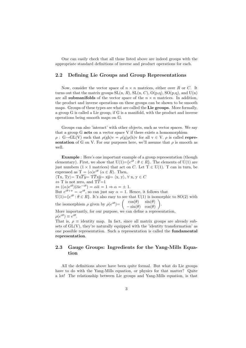
Example : Here’s one important example of a group representation (thoughelementary). First, we show that U(1)=eiθ : θ ∈ R. The elements of U(1) arejust numbers (1× 1 matrices) that act on C. Let T ∈ U(1). T can in turn, beexpressed as T = (α)eiθ (α ∈ R). Then,〈Tx, Ty〉= TxTy= TTxy= xy= 〈x, y〉, ∀ x, y ∈ C⇔ T is not zero, and TT=1⇔ ((α)eiθ)(αe−iθ) = αα = 1 ⇒ α = ± 1.But eiθ+π = -eiθ, so can just say α = 1. Hence, it follows thatU(1)=eiθ : θ ∈ R. It’s also easy to see that U(1) is isomorphic to SO(2) with

the isomorphism ρ given by ρ(eiθ)=(

cos(θ) sin(θ)− sin(θ) cos(θ)

).

More importantly, for our purpose, we can define a representation,ρ(eiθ) ≡ eiθ.That is, ρ ≡ identity map. In fact, since all matrix groups are already sub-sets of GL(V), they’re naturally equipped with the ’identity transformation’ asone possible representation. Such a representation is called the fundamentalrepresentation.

2.3 Gauge Groups: Ingredients for the Yang-Mills Equa-tion

All the definitions above have been quite formal. But what do Lie groupshave to do with the Yang-Mills equation, or physics for that matter? Quitea lot! The relationship between Lie groups and Yang-Mills equation, is that

3

different Lie groups give rise to different Yang-Mills equations, and these inturn describe the various forces in the standard model of physics. The Lie groupthat corresponds to a given Yang-Mills equations, or informally, the group thatprovides the ’ingredient’ for a given Yang-Mills equation for a particular forceunder consideration, is called the gauge group (or symmetry group). It’dbe ideal at this stage to give a brief preview of what we’ll be talking about lateron, in order to get comfortable with the idea of ’associating’ a Lie group with aparticular force. In addition, it will turn out that the Yang-Mills equations arelinear if and only if the associated gauge group is abelian. But we’re gettingahead of ourselves here. Let’s first work out an example.

Electromagnetism has U(1) as its gauge group. From our work above, weknow that we can consider U(1) as forming a unit circle in the complex plane.The electroweak force has as its gauge group SU(2) × U(1), while the strongnuclear force (i.e. Strong force) has SU(3) as its gauge group. Finally, the gaugegroup of the standard model is SU(3)× SU(2)× U(1). One of the attempts ofthe so called grand unified theories (GUTs) is putting physics on a ”largerand nicer” gauge group by treating SU(3) × SU(2) × U(1) as a subgroup ofsome ”larger and nicer” group such as SU(5).

One can also explore the connection between gauge groups and physicalcharges (both electric and ’colour’ charges). The intimate connection betweenthem is that the physical charge of a particle is described naturally by selectinga particular representation for the gauge group in question. This is one of thepowers of using group theoretical methods to build models of particle physics.Before moving on, let’s take a closer look at one example of a gauge group,namely the gauge group for electromagnetism U(1).

Example : We first define what seems to be quite a ’natural’ representationρn of U(1) (ρn: U(1) → GL(C)). Define ρn(eiθ)v = einθv, where v ∈ C andn ∈ ℵ. First, we show that this is indeed a representation. This is easy to dosince ρn(eiθeiφ) = einθeinφ. So indeed, ρn is a homomorphism, and noting thateinθ acts on any v, by effecting a rotation of nθ on v, we see that it’s an elementof GL(C) indeed. Hence, ρn is a representation of U(1) on C. From quantummechanics, we know that electric charges are quantized. That is, a particle canonly have nq charges where q is the elementary charge, which we take to bethe charge of an electron for simplicity (we won’t go into quark model here forsimplicity, which states that 1

3q is the true ’elementary’ charge). Then, notethat a particle with charge nq transforms according to the representation ρn ofU(1) on C. Namely, say we move a particle of charge nq around a loop γ inspacetime, then quantum mechanics tells us that its wavefunction is multiplied

by a certain phase, which is an element of U(1), namely by e− i

h nq(∮

γA)

, whereA is a vector potential. Now, the numerical values of q and h are dependent onthe choice of units, which can be arbitrary. We choose our units such that h =

q = 1. This is often called the ”God given units”. We then have e−in

∮γ

A=

4

ρn(e−i

∮γ

A), with e

−i∮

γA ∈ U(1).

One of the main goals of gauge theory is to generalize ideas such as this toother gauge groups corresponding to different forces.

3 Lie Algebras

We interrupt our study of Lie groups at this juncture, to introduce an equallyimportant notion called Lie Algebras.

3.1 Preliminary Definition

We start off by defining what a Lie Algebra is. Let G be a Lie group. Thena Lie algebra of G, denoted g, is the tangent space of the identity element ofG. Note that since G is a manifold, above is well-defined. One heuristic wayof thinking about a Lie algebra of a Lie group G is to view it as a space oftangent vectors to paths in G that originate at the identity element of G. Notethat this is a vector space with same dimension as G. It will turn out that amore abstract definition can be given for Lie algebra. Rather than introducingit right away, we go through an example, and some algebraic formalities to letit come out ’naturally’.

3.2 Lie Algebra of SO(3)

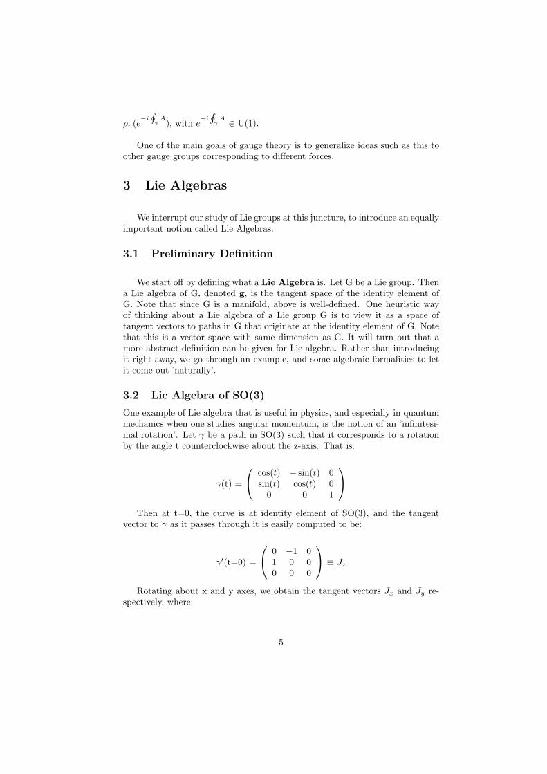
One example of Lie algebra that is useful in physics, and especially in quantummechanics when one studies angular momentum, is the notion of an ’infinitesi-mal rotation’. Let γ be a path in SO(3) such that it corresponds to a rotationby the angle t counterclockwise about the z-axis. That is:

γ(t) =

cos(t) − sin(t) 0sin(t) cos(t) 0

0 0 1

Then at t=0, the curve is at identity element of SO(3), and the tangent

vector to γ as it passes through it is easily computed to be:

γ′(t=0) =

0 −1 01 0 00 0 0

≡ Jz

Rotating about x and y axes, we obtain the tangent vectors Jx and Jy re-spectively, where:

5

Jx =

0 0 00 0 −10 1 0

Jy=

0 0 10 0 0−1 0 0

These are all in the Lie algebra of SO(3), and we denote it by so(3). It’s

important to keep in mind that we are interested in paths that lie in SO(3)and not in R3!. After all, SO(3) is a manifold (since it’s a Lie group), andwhen we say a ’path’ in SO(3), we can informally think of it as being a stringof matrices in SO(3) ”sewn” together along this path, such that as one movesalong the path, the entries of the matrices change continuously (i.e. ’smoothly’).

Now that we have obtained these matrices representing ’infinitesimal rota-tions’ about the identity element, what we now show is an important conceptthat one can obtain matrices describing finite rotations in R3 by using expo-nentials of linear combinations of the infinitesimal rotations Jx, Jy, and Jz.

As we know from classical linear algebra, the ’exponential’ of an n × n realmatrix A is defined by the ’Taylor Series’ of it:

exp(A) = 1 +A+ A2

2! + A3

3! + . . .

Before moving on, we need to prove that above series actually makes sense.That is, it converges to some matrix S with the same dimensions as A. Thisproof would be rather tedious and long, so we carry out only the key parts ofit:

Claim: exp(A) is well defined in the sense above.Proof : We define a norm ‖A‖ of n × n real matrix A as follows:

‖ A ‖≡ sup‖Ax‖‖x‖ ,

where the supremum is taken over all non-zero vectors v. Also, note that ‖ . ‖on the right hand side of above equality is the standard norm. Then by linearity,it’s easy to show that we can project all the vectors onto the unit sphere so that

‖ A ‖= sup ‖ Ay ‖,where the supremum is taken over all unit vectors y. Then this norm obeys theproperties of norm which are:(i) ‖ αA ‖=| α |‖ A ‖(ii) ‖ A+B ‖≤‖ A ‖ + ‖ B ‖(iii) ‖ A ‖= 0 ⇔ A = 0, and ‖ A ‖> 0 otherwise.It also satisfies one further property which is that(iv) ‖ AB ‖≤‖ A ‖‖ B ‖Now, we define the sequence < sn > where

sn ≡∑n

k=0Ak

k!then for m ≥ n, we have

‖ sn − sm ‖ = ‖ An+1

(n+1)! + ...+ Am

m! ‖≤‖ An+1

(n+1)! ‖ +...+ ‖ Am

m! ‖, (by (ii))

6

≤ ‖An+1‖(n+1)! + ...+ ‖Am‖

m! , (by (iv))In the last line above, we have ‖ sn − sm ‖ reduced to the tail-end of the usualexponential series, with ‖ A ‖ treated as just a number. And we know that theTaylor series for the exponential function converges. Hence, this means that∀ε > 0,∃Nε ∈ N such that ‖ sn − sm ‖ ¡ ε, ∀n,m ≥ Nε. Hence, it follows thatsn is a Cauchy sequence, and by the completeness of Cn (or Rn, dependingon the space we’re working with), the sequence converges, which means that wecan find some n × n matrix S such that ‖ S ‖= limn→∞ ‖ sn ‖. This provesthat the exponential of the square matrix is well-defined indeed.

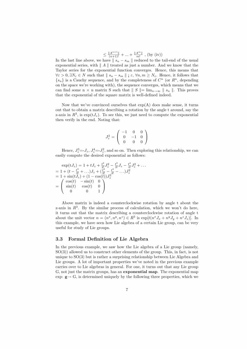
Now that we’ve convinced ourselves that exp(A) does make sense, it turnsout that to obtain a matrix describing a rotation by the angle t around, say thez-axis in R3, is exp(tJz). To see this, we just need to compute the exponentialthen verify in the end. Noting that:

J2z =

−1 0 00 −1 00 0 0

Hence, J3

z =-Jz, J4z =-J2

z , and so on. Then exploring this relationship, we caneasily compute the desired exponential as follows:

exp(tJz) = 1 + tJz + t2

2!J2z − t3

3!Jz − t4

4!J2z + . . .

= 1 + (t− t3

3! + . . .)Jz + ( t2

2! −t4

4! − . . .)J2z

= 1 + sin(tJz) + (1− cos(t))J2z

=

cos(t) − sin(t) 0sin(t) cos(t) 0

0 0 1

Above matrix is indeed a counterclockwise rotation by angle t about the

z-axis in R3. By the similar process of calculation, which we won’t do here,it turns out that the matrix describing a counterclockwise rotation of angle tabout the unit vector n = (nx, ny, nz) ∈ R3 is exp[t(nxJx + nyJy + nzJz)]. Inthis example, we have seen how Lie algebra of a certain Lie group, can be veryuseful for study of Lie groups.

3.3 Formal Definition of Lie Algebra

In the previous example, we saw how the Lie algebra of a Lie group (namely,SO(3)) allowed us to construct other elements of the group. This, in fact, is notunique to SO(3) but is rather a surprising relationship between Lie Algebra andLie groups. A lot of important properties we’ve noted in the previous examplecarries over to Lie algebras in general. For one, it turns out that any Lie groupG, not just the matrix groups, has an exponential map. The exponential mapexp: g→ G, is determined uniquely by the following three properties, which we

7

won’t prove here as they are beyond the scope of this paper, and would onlylead us astray. The three properties are:

(i) exp(0) = identity element of G. (Here, 0 is the identity element of theLie algebra of the Lie group G).

(ii) exp(sx)exp(tx) = exp((s+t)x), ∀ x ∈ γ and s, t ∈ R. (where γ is anycurve that originates from the identity element of G).

(iii) ddt exp(tx) |t=0 = x.

Above properties match the ’regular’ properties of the exponential functionin C that many of us are more familiar with. As a consequence of above prop-erties and the inverse function theorem, it turns out that exp can map anysufficiently small open neighbourhood containing the identity element 0 of Liealgebra g onto an open set that contains the identity of G. Furthermore, anyelement of the identity component of G is the product of elements of theform exp(x). An identity component is a connected component that containsthe identity element of the group. Then as we mentioned above, in some sense,most of the structure of a Lie group is encoded in the structure of its Lie algebra.We elaborate this very important idea further.

To do so, we first abstractly define a Lie algebra. First, we denote theLie bracket (or commutator) by [·, ·]. Then, we define Lie algebra to beany vector space g that is equipped with a map [·, ·]: g×g → g. such that thefollowing three properties are satisfied (properties of Lie brackets):

(i) [v,w] = -[w,v], ∀ v,w ∈ g.(ii) [u, αv + βw] = α[u,w] + β[u,w], ∀ v,w, u ∈ g, and scalars α and β.(iii) (Jacobi identity): [u,[v,w]]+[v,[w,u]]+[w,[u,v]]=0, ∀ u,v,w ∈ g.

(Note: α and β are real numbers for Lie algebra g that forms a real vectorspace. They are complex numbers if g forms a complex vector space.)

We can also define homomorphism between one Lie algebra to another.This is quite naturally defined as a linear map f from the Lie algebra g to theLie algebra h such that f([v,w]) = [f(v),f(w)], ∀ v,w ∈ g. Of course, f is anisomorphism if it’s one-to-one and onto.

Note that these notions that we’ve been talking about here have striking re-semblances with Lie brackets defined on vector fields. Indeed, given a manifoldM, the space of all vector fields on M is a Lie algebra with the standard Liebracket defined for vector fields on M. The difference here is that it’s an infinitedimensional Lie algebra where as for the Lie groups we’ve been considering thusfar, deal with finite dimensions.

We have seen that every Lie group has a Lie algebra. But what we haven’tmentioned so far is that every homomorphism ρ: G → H (where G and H areLie groups) determines an associated homomorphism dρ: g → h between theLie algebra g of G and the Lie algebra h of H. More specifically, dρ is thepushforward of tangent vectors at the identity of G. That is,

8

dρ = (ρ)∗ : TidentityG→ TidentityH.Although we choose to omit the proof here, above indeed forms a Lie algebra.

3.4 Application to Physics

Our goal, from the beginning, was to see how Lie algebras and Lie groupsare used in various parts of physics. We have developed sufficient amount ofdefinitions and are now in a position to do just that. But before doing so, weneed just one more formal definition, namely, the notion of representation of Liealgebras.

Lie group representations determine Lie algebra representations and viceversa. In the spirit of the definition of representation of a Lie group G on a vectorspace V, we define a representation of a Lie algebra g on a vector space V tobe a Lie algebra homomorphism f: g → g[(V), where g[(V) is the Lie algebra ofall linear operators on V, with the standard definition of a commutator. Recallthat we have stated exp is well defined for any Lie groups. A very importantfact about Lie algebras is that if one starts with a representation f: g → g[(V),one can ’exponentiate’ it to obtain a representation ρ: G → GL(V) with dρ =f, given that G is simply connected.

Example After all the formalities, we can now give a basic sketch of applica-tion of Lie algebras in physics. Most of the mathematics in quantum mechanicsare deeply rooted in the infinite dimensional Hilbert space H. Under rotationsymmetry in 3 dimensional space, there exists a unitary representation U ofSU(2) on H. And as we mentioned above, this representation naturally givesrise to a representation dU of the Lie algebra su(2) on H. We can then definedU(ix) ≡ idU(x) for any x ∈ su(2). Physically, the operator dU(σz

2 ) on H iscalled the angular momentum about the z-axis, where σi is a Pauli Matrixabout the i-axis. The precise entries of this matrix is not important for ourpurpose here.

Let’s elaborate on this further. In quantum mechanics, a system has itsassociated wavefunction, which encodes all the information about the system,including the measurement values of any observables one might want to mea-sure. Let ψ be a wavefunction for a particle. ψ ∈ H for physical particles.The statistical expected value of some observable A of a particle is given by:< ψ,Aψ > with < f, g > being the usual inner product on a Hilbert space(i.e.

∫(fg), integral taken over all physical space). Then according to the for-

malism we’ve developed above, it follows that the z-component of the system’sangular momentum about the z-axis is just < ψ, dU(σz

2 )ψ >. Generalizing thisconcept, the angular momentum about any unit vector v ∈ R3 is given by theoperator dU(vi/sigmai/2), (where /sigmai denotes the Pauli Matrix definedin the appendix). In a similar fashion, we can use other symmetry groups todescribe other observables. So for instance, translation in space gives momen-tum, and translation in time gives energy. This shouldn’t be a surprising result

9

considering that even in classical mechanics, momentum p and energy E exhibitrelationships: p = F · (4d) and E = F4(t), where 4t and 4d denote time in-tervals and displacements through which the force F is applied. These intimateconnections exhibited between time and Energy, and space and momentum, aretwo of the fundamental relationships in physics, which crop up again and againin such phenomena as Heisenberg’s uncertainty principle, which again couplesenergy with time interval, and momentum with displacements. We see here thatthese relationships come up in group theoretical treatments of physical modelsas well.

4 Bundles: Ingredients for Gauge Fields

In order to reach our goal of constructing Yang-Mills equations, we are in-evitably forced to study the algebraic concept of bundles, and gauge transfor-mations. Gauge transformations, in particular, are important in many physicalmodels. For instance, even in classical electromagnetism, Maxwell’s equationsdescribing any charge and current configurations can be simplified from a com-putational perspective, if we ’gauge transform’ the Maxwell’s equations. InYang-Mills equations, this concept becomes especially important, as we’ll see.Here, we present only the very basic aspects of bundles and gauge transforma-tions that pertain to our purposes.

4.1 Bundles: Preliminaries

Gauge theory deals with general fields on spacetime. What exactly are these’general fields’? To describe them, we need to understand a bit about vectorbundles. First, we note the important fact that a vector field on a manifoldM assigns to each point p ∈ M, a tangent vector which lives in the tangentspace TpM at p on M. This means that since the vector field assigns vectorsnot in some fixed single vector space, we cannot naively compare two tangentvectors at two different points of M, because they live in different spaces. This,in turn, implies that we cannot define a differentiation of a vector field on M thesame way we define differentiation of real-valued functions in Euclidean space.This seemingly innocent fact has far reaching consequences in Gauge theory. Ingauge theory, fields are different ’segments’ of the ’bundles’ or the ’collection’of the tangent spaces of M, which assign to each point in spacetime a vector inthe vector space to which the point belongs to. What is needed for formation ofYang-Mills equations is a method to compare vectors in these different tangentvector spaces, which is a field called a ’connection’. Yang-Mills equations turnout to be the equations for this connection itself, as we’ll see after we familiarizeourselves with some algebraic formalisms.

A bundle is an algebraic structure consisting of two manifold E and M, andan onto map π : E → M. For example, M can be a real line, and E can be R2

10

plane, with π being the standard projection map π(x,y)=x, ∀ (x,y) ∈ R2. WithE, M, and π taking roles in the sense of this example, E is called a total space,M is called base space, and π is not surprisingly called the projection map.Furthermore, for each p ∈ M, we define Ep = q ∈ E : π(q) = p to be a fiberover p. Then it follows that the total space E can be ’built up’ from its fibers,E =

⋃p∈M Ep. For this reason, we often refer to E as being a ’bundle’, or a

’bundle’ over M. In physical applications, M becomes a Euclidean space or aspacetime.

A tangent bundle of a manifold M can be defined as follows. In a tangentbundle, the total space TM is just TM =

⋃p∈M TpM , where TpM is the tangent

space at p of M. In this bundle, the project map π is naturally defined to beπ(v) = p, where v ∈ TpM and p ∈ M . Hence, the fiber over p is TpM . Butthis doesn’t guarantee that TM is a manifold because π needs to be guaranteedto be smooth. To do so, we use the idea that specifying a point in TM is thesame as specifying a point p in M together with a vector v ∈ TpM . And sinceboth M and TpM look locally like Rn (where M is an n-dimensional manifold),TM should locally look like Rn ×Rn. Let’s make this idea more precise:

Let M be a n-dimensional smooth manifold over Rn. Let φα : Uα → Rn

denote a chart of M, with Uα being an open set on M. Define a subset of TM :Vα = v ∈ TM : π(v) ∈ Uα. Now, for each v ∈ TM , since TM =

⋃p∈M TpM ,

∃ p ∈ M such that v ∈ TpM (i.e. v is a tangent vector at p on M). Henceπ(v)=p, and since M is a manifold, there exists an open set Uα that contains p.Hence v ∈ Vα for some Vα of TM . Next, define maps ψα : Vα → Rn × Rn byψα(v) = (φα(π(v)), (φα)∗v). We can think of (φα)∗v as a vector in Rn thoughit is really a tangent vector to Rn. We induce a ”natural” topology to TM bydefining it to be collection of Vα’s. That is, a set of TM is open if and only if itis one of Vα’s. Then, note that φα(π(Vα)) ⊆ Uα and is open in Rn because φα

is continuous, and that φα(Vα) is also open in Rn since the pushforward φα issmooth. Hence, ψα(Vα) is open in Rn ×Rn. Although it’s tedious, it’s easy tocheck that ψα’s are charts for TM . Hence it follows that in this setting, TM isa manifold. It’s also easy to check that π is a smooth map here. One can easilyconvince oneself of this fact by considering a smooth curve lying on M, and thetangent vector to the curve varying in a ’continuous’ manner as one traversesthe curve.

We define a trivial bundle over M with standard fiber F to be the Carte-sian product E = M×F , with the projection map π(p, f) = p, ∀ (p,f) ∈M×F .That is, a trivial bundle amounts to the construction of a bundle by choosing adesired base space along with an explicit fiber of your desire. Note that we cangive a ’canonical’ diffeomorphism between each fiber and F, by sending (p,f)∈ Ep to f ∈ F . This property turns out to be unique to trivial bundles.

Bundles that are not ’globally’ trivial, but rather ’locally’ trivial turn out tobe more useful in many physical models. Informally, as you may have guessed, an

11

a bundle is ’locally’ trivial if it looks trivial in sufficiently small neighbourhoodof any given point. Examples include cylinders (trivial over S1 with standardfiber R) and Mobius strip over a ’small’ portion of S1. We can in fact, makethis definition more precise. But first, we need to introduce some more notions.

Given two bundles, π : E → M and π′ : E′ → M ′, a morphism from thefirst to the second is a map ψ : E → E′ together with a map φ : M →M ′ suchthat ψ maps each fiber Ep into the fiber E′φ(p). In other words, a morphism”transforms” one bundle into another. A morphism is called an isomorphismif φ and ψ are both diffeomorphisms.

Suppose we’re given two bundles π : E → M and π′ : E′ → M ′. We nowshow that the maps ψ : E → E′ and φ : M → M ′ are a bundle morphism ifand only if π′ ψ = φ π. First, suppose that ψ : E → E′ and φ : M → M ′

are a bundle morphism. Then for y ∈ Ep, π′ ψ(y) = π′(z) = φ(p) = φ π(y),where z ∈ E′φ(p) by definition, and p = π(y). Hence π′ ψ = φ π. Conversely,say π′ ψ = φ π. Then for y ∈ Ep; π′ ψ(y) = π′(z) = p′ where z ∈ E′p′ ,⇒ ψ(y) ∈ E′p′ . On the other hand, φπ(y) = φ(t) = p′, where t ∈M ⇒ y ∈ Et,hence ψ maps Ep to E′φ(p). Hence, we’ve proven what we set out to do.

Furthermore, it’s easy to show that for a given ψ defined for a morphism,if φ and φ′ are two corresponding maps for the base space, then φ = φ′. Tosee this, note that since we have a morphism, φ′ ψ = φ π = φ′ π by ourprevious work above. Then now, the rest is very simple, because π is onto map,so φ(p) = φ′(p),∀p ∈ E,⇒ φ ≡ φ′. Hence, ψ uniquely determines φ. For thisreason, we can be quite lax and call ψ to be the ’bundle morphism’.

One very useful and familiar example of a bundle morphism is induced bythe pushforward of tangent vectors. Let φ : M → M ′ denote a map betweenmanifolds M and M’. Then we have the pushforward φ∗ : TpM → Tφ(p)M

′. Wealso know that TM =

⋃p∈M TpM , and TM ′ =

⋃p′∈M ′ Tp′M ′. Then we see

that in fact, φ∗ : TM → TM ′, with φ being smooth ⇒ φ∗ being smooth. Henceφ∗ : TM → TM ′ is a bundle morphism.

For a bundle π : E → M and a submanifold S ⊆ M , a restriction to S isdefined by taking E |s= q ∈ E : π(q) ∈ S as the total space, and taking S asthe base space with π restricted to E |s as the projection. Now, we’re finally in aposition to give a precise formulation of local triviality. A bundle π : E →M iscalled locally trivial if for each p ∈M , there exists an open neighbourhood Uof p, and a bundle isomorphism φ : E |U→ U × F , such that it sends each fiberEp to the fiber p ×F . Such a φ is called a local trivialization, and a sectionof E |U is called a section of E over U. When we use charts on manifolds, weare using the concept of ’local analysis’. In a similar spirit, local trivializationof a bundle simplifies our analysis of bundles by allowing us to perform a ’localanalysis’ of the bundle.

12

Before moving on, we note the important fact that for any smooth n-dimensionalreal manifold M, the tangent bundle π : TM → M is locally trivial. Ratherthan giving a formal proof, we can, as physicists, intuitively see this as follow-ing. Pick a point p on a manifold M, then via a chart local to that region ofM, we can find some open subset U of M containing p. Now, for TpM , we candefine a map φ(vp) = (p, vp), and it’s quite clear to see that this is a bundleisomorphism, with the standard fiber being Rn, with vp tangent vector in p inRn of course.

4.2 Vector Bundles

We now confine our attention to specific kind of bundles, namely the vectorbundles. Vector bundles are what we really need in formulation of Yang-Mill’sequations and mathematical physics in general.

An n-dimensional real vector bundle is a locally trivial bundle π : E →Msuch that each fiber Ep is a n-dimensional vector space, with the additionalrequirement that for each p ∈ M, there exists a neighbourhood U ∈ M of p anda local trivialization φ : E |U→ U × Rn that maps each fiber Ep to the fiberp×Rn linearly. In this situation, we say that the trivialization is fiberwiselinear. The definition of complex vector bundle is exactly the same as this oneexcept that we replace Rn with Cn. What we’ll now describe for real vectorbundles are equally applicable to complex vector bundles with the modificationmentioned above.

We first show that TM of M is a vector bundle. We already showed above(at least heuristically), that TM is a trivial bundle. Let Ep be a fiber overp ∈ M, where M is an n-dimensional real smooth (as always) manifold. Weknow that TpM is isomorphic to Rn (i.e. they ”look” alike). Now then, letφ(vp) = (π(vp), vp). Then, with real scalars α and β, we have:φ(αvp + βwp) = (p, αvp + βwp) = (p, αvp) + (p, βwp) = φ(αvp) + φ(βwp) wherewe define ”componentwise addition” above. (p, vp) + (q, wq) where p6=q simplywouldn’t make sense. It’s easy to see that φ is a bundle isomorphism, and hencewe conclude that the tangent bundle of a manifold is a vector bundle indeed.

We interrupt our development of formalisms to inject an important com-ment at this junction. Physics should be ’invariant’ under any choice of a localcoordinate system on spacetime. After all, how nature behaves shouldn’t bedependent on what we, as observers of phenomena, pick as our tools to describethem. In the same spirit then, physics is invariant under any local trivializationof whatever vector bundles under consideration when we describe physical fieldsin spacetime. This is the principle of gauge invariance and we’ll elaborate onthis in more detail later on. But first, let’s return to development of some moreformalisms.

13

Given two vector bundles π : E → M and π′ : E′ → M ′, a vector bundlemorphism from first bundle to the second bundle is a bundle morphism ψ :E → E′ such that its restriction to each fiber Ep of E is linear. That is, themorphism restricted to each fiber Ep ”preserves” the linearity of the vector spaceEp.

Finally, we are one step closer to completing a toolkit to describe fields inspacetime. As aforementioned, physical fields, whether they be electromagneticfields, or gravitational fields, can be described as ’sections’ of vector bundles. Asection of a bundle π : E →M is simply a function s : M → E so that ∀p ∈M ,s(p)∈ Ep. Physically, this means as we ’traverse’ in any curve γ on the basespace M (which is a smooth manifold), sγ traverses through Esγ . So a sectionassigns to each point p ∈ M, a specific vector in the fiber over that point. If youhave a trivial bundle E = M × F with a standard fiber F, then a section of Eis just a function f : M → F such that s(p) = (p, f(p)) ∈ Ep. Or we can definea function f instead, in which case it would induce a corresponding section forthe trivial bundle. It’s physically obvious that a section of the tangent bundleis a vector field, and we’ve known all along that a vector field on spacetimemanifolds, describe physical fields. Evidently, a physical field can be treated asa ’section’. The subtlety present here is that when we think of vector fields inthe Euclidean space, we’re really looking at vector fields defined in one vectorspace, while sections describe vectors, or ”little arrows” if you will, in differentspaces, namely the fibers.

We know that certain forces in nature obey the superposition principle. Thatis, two fields add up vectorially to form the field that we physically observe innature (i.e. the resultant field). Vector fields can then be added. In a similarspirit then, it only makes sense that sections should have the ability to withstandadditions as well. Indeed, they do. Given a vector bundle E over a manifold M,and sections s and s’ of E, we define addition of sections as:(s+s’)(p) = s(p) + s’(p)We also define multiplication of sections by functions on M as (where f∈ C∞(M): (fs)(p) = f(p)s(p). Γ(E) denotes the set of all sections of E.

Recall that for a vector bundle, Ep is a vector space with all the fibershaving the same dimensions. Now, let’s imagine the following situation. Wehave a smooth curve γ in the total space E (remember that E is a smoothmanifold), then at some instant t0, γ(t0) ∈ E−→x . And we have a basis for thevector space E−→x at this instant. Then in some infinitesimal time dt later, wehave γ(t0 + dt) ∈ E−→x +d−→x , and at this instant, each of the basis vectors forthe vector space E−→x has been ”perturbed” little to form a basis for the newfiber E−→x +d−→x . We can consider this as a ”moving frame” in which the basisvectors vary smoothly as we traverse through different sections. Indeed, we canmake this notion more precise. Given a vector bundle E, basis of sectionsof E is the set of sections e1, . . . , en such that any section s ∈ Γ(E) can be

14

uniquely expressed as a sum s = siei (with the Einstein summation notationbeing used here), where si ∈ C∞(M). Although we will not prove here, it turnsout that a vector bundle has a basis of sections if and only if it’s isomorphic toa trivial bundle. Note, however, that vector bundles, by definition, are locallyisomorphic to trivial bundles. Hence, when we perform a local analysis, we canpick a basis of sections over a sufficiently small neighbourhood of any point inthe base space.

4.3 Construction of Vector Bundles useful in General Rel-ativity

We’ve seen above some of the correspondences between vector spaces andvector bundles. This is no coincidence since a vector space is really a vectorbundle with base space equal to a single point. That is, we have a very ’direct’isomorphism here. We now develop some notions for vector bundles that arefamiliar to us in the vector space setting.

Say we have a vector bundle E over M. Each fiber Ep is a vector spaceand hence it has a well-defined dual space E∗p . Then we can construct what’scalled a dual vector bundle E∗ over M as follows. We let its total spaceto be E∗ = ∪p∈ME∗p , and let the projection π : E∗ → M map each E∗p to p.Hence E∗p is the fiber over p∈ M. It can be shown that E∗ is indeed a manifoldand that there’s a local trivialization of E∗ that’s fiberwise linear. Hence E∗

is a vector bundle indeed. An important example of a dual vector bundle, forcomputational purposes, is the cotangent bundle T ∗M of a manifold M. Forthis dual vector bundle, its fiber of a point is the cotangent space at the point,and a section of T ∗M is a 1-form on M.

Let E and E’ be two vector bundles over M. A direct sum vector bundleE

⊕E′ over M has as its fiber over p, Ep

⊕E′p. This is a ”natural” way

to define direct sum of two objects indeed. In a similar spirit, the tensorproduct vector bundle E

⊗E′ over M has as its fiber over p, Ep

⊗E′p.

Both the direct sum vector bundle and the tensor product vector bundle areindeed vector bundles.

Now, we reveal perhaps one of the more important constructions that’s use-ful in study of gauge fields, and it’s the object called a ”G-bundle”. Here’s howwe construct it. First, we start off with some essential ingredients. We have asmooth manifold M along with the open cover Uα of M. In addition, we selecta vector space V, group G, and a representation ρ of G on V, all of which areof our own choosing. So summarizing, our ingredients are: M, Uα, V, ρ,G.Now, we construct a total space as follows. Consider T ≡

⋃α Uα × V . Now,

we ’identify’ elements in T as follows. Two points (p,v) ∈ Uα × V and (p,v’)∈ Uβ ×V are considered ’equal’ if v = ρ(gαβ(p))v′, where gαβ : Uα

⋂Uβ → G is

15

a transition function. We denote above condition as v = gαβv′ for simplicity.

Informally, what we’re saying is that for each point p ∈ M, we also have anassociated group element g ∈ G. And associated with this g acts on elementsof V. If this g acts on v’ to get v, then we will only put one of them in thefiber over p, since there’s a way to obtain the other vector via the interactionbetween M and G. Now, there are two constraints on this procedure in order toinsure consistencies.1.) gαα ≡ 1 on Uα: For otherwise, we’d have to identify (p,v) and (p, gααv),

both of which lie in Uα × V . But we don’t want to identify two differentelements in the same trivial bundle. This constraint prohibits this situation.

2.) Cocycle condition - gαβgβγgγα ≡ 1 on Uα

⋂Uβ

⋂Uγ . This allows identi-

fication of (p,v), (p, gαγv), and (p, gβγgγαv) as one element (p, gαβgβγgγαv).It turns out that other similar consistency conditions follow from the require-ments 1) and 2) above. To finalize our construction of this ”special” vectorbundle, we denote the equivalence class [p, v]α to be the ”point” of E (ratherthe representative) corresponding to (p,v) ∈ Uα × V . We then define the pro-jection π : E → V by π[p, v]α = p. Then the fiber Ep is the set of all points inE of form [p, v]α. So we’ve finally constructed the fibers! Due to the conditions1) and 2) imposed above, it turns out that π : E →M is a vector bundle. Thiskind of vector bundle is what we called a G-bundle above. The group G iscalled the gauge group of bundle, and V is called the standard fiber. Asyou recall, we’ve already defined what a gauge group is before. Physical gaugefields are described by sections as mentioned before. More specifically, they’rethe sections of G-bundles, and by varying the group G, we can describe differentforces. This was exactly what we said a gauge group is all about in the previoussections.

5 Gauge Transformations

5.1 Gauge Theory and the Standard Model

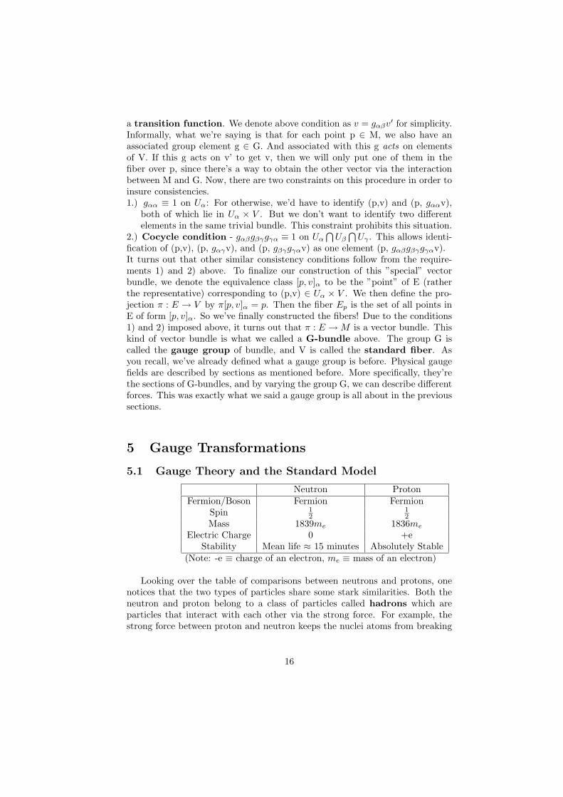
Neutron ProtonFermion/Boson Fermion Fermion

Spin 12

12

Mass 1839me 1836me

Electric Charge 0 +eStability Mean life ≈ 15 minutes Absolutely Stable

(Note: -e ≡ charge of an electron, me ≡ mass of an electron)

Looking over the table of comparisons between neutrons and protons, onenotices that the two types of particles share some stark similarities. Both theneutron and proton belong to a class of particles called hadrons which areparticles that interact with each other via the strong force. For example, thestrong force between proton and neutron keeps the nuclei atoms from breaking

16

apart by overcoming the electric repulsion between any two protons clusteredin the nuclei. To account for some of the properties of protons and neutrons,Heisenberg introduced the notion of isospin. Using this notion, if we ignore allthe interactions between a proton and a neutron resulting from any force otherthan the strong force, then the two particles can be considered as being merelytwo different states of a single particle, which we call a nucleon.

There are two different spins that a nucleon can have. A proton is arbitrar-ily assigned a ’isospin-up’ state which is represented by a unit vector in C2,(

10

), while the neutron is assigned the ’isospin-down’ state,

(01

). For this

reason, we say that nucleon is an isospin doublet. There are different ’spin’representations of SU(2), which are useful in describing different spin states ofparticles, which we won’t go into much detail here.

In the standard model of physics, one makes a distinction between a forceand an interaction. Every force is carried by a force carrier particle suchas photons, gluons, and pions (for strong force). The result of force carried bythese mediator particles from one particle to another results in the ’interaction’between the two particles. There are three pions, each with a positive, negative,or a neutral electric charge. Once again, assuming that the strong force is theonly force present, these three pions can be described as three different statesof a single particle, the pion. These transform according to so-called ’spin-1’representation of SU(2), and the isospin triplet.

Describing the dynamical aspects of a particle requires more than theirisotropic spin considerations. We need to analyze the ’matter wave’ represen-tation of a particle according to quantum mechanics for a full understandingof the dynamics. For example, for a nucleon, we have a ”field” (i.e. matterwave) ψ : R4 → C2 on the Minkowski spacetime (C2 because a nucleon is a’doublet’), while for a pion we have the ’field’ φ : R4 → C3. But the spins ofparticles depend on the polarization direction of the external force field suchas the electromagnetic field. That is, a spin is either up or down parallel tothe polarization axis of the external magnetic field that’s used to ’measure’ thespin. This observation, along with the fact that SU(2) is S3 as a manifold, tellsus that if we act on any valid fields φ and ψ defined above by an element g ∈SU(2), so that we have ψ′(x) = gψ(x) and φ′(x) = gφ(x), then both ψ′ andφ′ are also valid matter waves on Minkowski spacetime. Here, g ∈ SU(2) actsaccording to spin-1/2 and spin-1 representations, whose actual forms are not ofinterest to us here.

In their paper published in 1954, C.N. Yang and R. L. Mills have investi-gated the conservation of isotopic spin and isotopic gauge invariance. What theynoticed was that as mentioned before, when strong force is the sole force underconsideration, distinguishing between a neutron and a proton is a purely arbi-trary process. But at one space-time point, if one chooses what to call a proton

17

and what to call a neutron by assigning the aforementioned spins, then one isnot able to swap the labels on the two particles at other spacetime points. Yangand Mills thought that this was inconsistent with the localized field conceptthat underlies the usual physical theories; that this seemingly arbitrary choiceat one point in spacetime results in globally affecting the physics of the systemin the spacetime bothered them. Hence, they searched for the field equationsthat possess more symmetry, namely, symmetries under transformations of theform:ψ′(x) = g(x)ψ(x), and φ′(x) = g(x)φ(x)where g:R4 → SU(2) is any function that’s SU(2)-valued on spacetime. This dif-ficult problem was solved by Yang and Mills by mimicking Maxwell’s equations,and resulted in an SU(2) ’gauge theory’ of various sorts of hadrons.

Standard model does not take into account gravity, and in fact, there arefundamental inconsistencies that arise when we try to combine general relativitywith quantum field theory. Currently, efforts are being put to develop newtheories to take gravity into account, and standard model serves as a basis forthese candidate theories.

5.2 Gauge Transformations for Vector Bundles

For calculations involved in Yang-Mills equations that we’ll perform lateron, we need to make the concept of a gauge transformation more precise forvector bundles. This is what we set out to do in this section.

Let V be a vector space. Then the linear functions from V to itself(T:V → V) are called endomorphisms and the set of all endomorphisms of Vis denoted End(V). It’s easy to see that End(V) is a vector space with usualdefinitions of addition of two linear functions on V and multiplication by anyscalar. It’s also an algebra with the product of two linear functions S and Tdefined by (ST)(v) = S(T(v)), where v ∈ V. Note that End(Rn) is the algebraof n× n real matrices with matrix multiplication as the product. In fact, moreuseful definition can be devised by using the basis of V and the dual basis ofV ∗. We can define End(V) to be V ⊗ V ∗.

Let E be a vector bundle over a manifold M. Then End(E) is called anendomorphism bundle of E, which is the bundle E ⊗ E∗. Let’s considerwhat this is saying in more detail. Given a fiber of End(E) over some a point p∈ M, the fiber is same as End(Ep) because End(E) ≡ E

⊗E∗ by definition, so

indeed over p, the fiber will be End(Ep) ≡ Ep

⊗E∗p . Therefore, for any section

T of End(E), we get a map from E to itself sending v ∈ Ep to T(p)v ∈ Ep,which is a vector bundle morphism. So in fact, the name ’endomorphism’ isquite fitting here since ’endomorphism’ in Greek, depicts the notion of sendingsomething inside itself, as is the case with End(E).

18

We need to define one more terminology before defining what ”gauge invari-ance” means rigorously. Say p ∈ Uα (with Uα defined as in G-bundle). Then Tlives in the group G (in G-bundle), if it’s of form [p, v]α 7−→ [p, gv]α for some g∈ G. Now we are finally in a position to define succinctly the notions of ”gaugeinvariance” and ”gauge transformations”. Let T ∈ End(E) and p ∈ M. ThenT(p) ∈ End(Ep) as we saw above. If T(p) lives in G, ∀ p ∈ M, then T is said tobe a gauge transformation. Ω denotes the set of all gauge transformations,and it’s easy, yet tedious, to show that it is a group with products and inversesdefined by:(gh)(p) = g(p)h(p)g−1(p) = (g(p))−1

Gauge theory’s based on the foundation that physical fields are sections of G-bundles, and that the systems of differential equations that govern the evolutionof the physical systems are gauge invariant. That is, if section s is a solutionfor the system of differential equations, then gs is also a solution for any g ∈ Ω.

6 Connections and Curvature for Vector Bun-dles: A step towards Yang-Mills Equations

In our course (APM421: General relativity), we’ve already encountered thenotions of connections and curvature. But how do these notions arise in thesetting of bundles, which are things we haven’t explicitly considered in ourcourse so far? In this section, we address and try to answer this question withminimum amount of formalism as possible, keeping in mind what we alreadyknow from our course.

6.1 Introduction to Connections for Bundles

”Differentiating” a section of a vector bundle is not as simple as differen-tiating any real valued smooth functions because a section assigns vectors indifferent fibers as one traverses along the base space. This, in turn, results inthe ”addition” of two vectors assigned by a section to be not well defined inmany situations. A ’connection’ is simply a way to differentiate sections as aresult of this complication. More specifically, a connection D on manifold M(base space) assigns to each v ∈ Vect(M) a function Dv : Γ → Γ satisfying thefollowing conditions:(i) Dv(αs) = αDvs (Linearity)(ii) Dv(s+ t) = Dvs+Dvt (Linearity)(iii)Dv(fs) = v(f)s+ fDvs (Leibnitz Rule)(iv) Dv+ws = Dvs+Dws(v) Dfs = fDvs

19

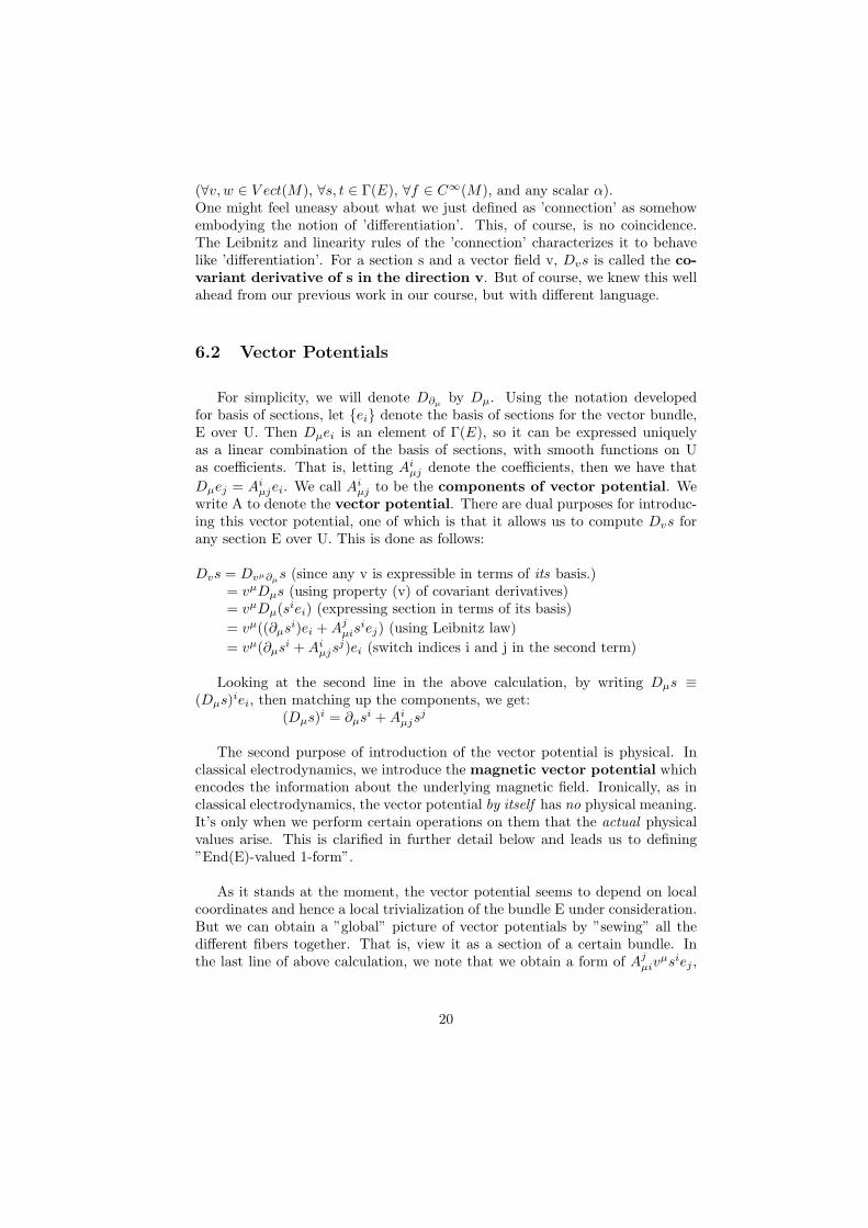
(∀v, w ∈ V ect(M), ∀s, t ∈ Γ(E), ∀f ∈ C∞(M), and any scalar α).One might feel uneasy about what we just defined as ’connection’ as somehowembodying the notion of ’differentiation’. This, of course, is no coincidence.The Leibnitz and linearity rules of the ’connection’ characterizes it to behavelike ’differentiation’. For a section s and a vector field v, Dvs is called the co-variant derivative of s in the direction v. But of course, we knew this wellahead from our previous work in our course, but with different language.

6.2 Vector Potentials

For simplicity, we will denote D∂µby Dµ. Using the notation developed

for basis of sections, let ei denote the basis of sections for the vector bundle,E over U. Then Dµei is an element of Γ(E), so it can be expressed uniquelyas a linear combination of the basis of sections, with smooth functions on Uas coefficients. That is, letting Ai

µj denote the coefficients, then we have thatDµej = Ai

µjei. We call Aiµj to be the components of vector potential. We

write A to denote the vector potential. There are dual purposes for introduc-ing this vector potential, one of which is that it allows us to compute Dvs forany section E over U. This is done as follows:

Dvs = Dvµ∂µs (since any v is expressible in terms of its basis.)

= vµDµs (using property (v) of covariant derivatives)= vµDµ(siei) (expressing section in terms of its basis)= vµ((∂µs

i)ei +Ajµis

iej) (using Leibnitz law)= vµ(∂µs

i +Aiµjs

j)ei (switch indices i and j in the second term)

Looking at the second line in the above calculation, by writing Dµs ≡(Dµs)iei, then matching up the components, we get:

(Dµs)i = ∂µsi +Ai

µjsj

The second purpose of introduction of the vector potential is physical. Inclassical electrodynamics, we introduce the magnetic vector potential whichencodes the information about the underlying magnetic field. Ironically, as inclassical electrodynamics, the vector potential by itself has no physical meaning.It’s only when we perform certain operations on them that the actual physicalvalues arise. This is clarified in further detail below and leads us to defining”End(E)-valued 1-form”.

As it stands at the moment, the vector potential seems to depend on localcoordinates and hence a local trivialization of the bundle E under consideration.But we can obtain a ”global” picture of vector potentials by ”sewing” all thedifferent fibers together. That is, view it as a section of a certain bundle. Inthe last line of above calculation, we note that we obtain a form of Aj

µivµsiej ,

20

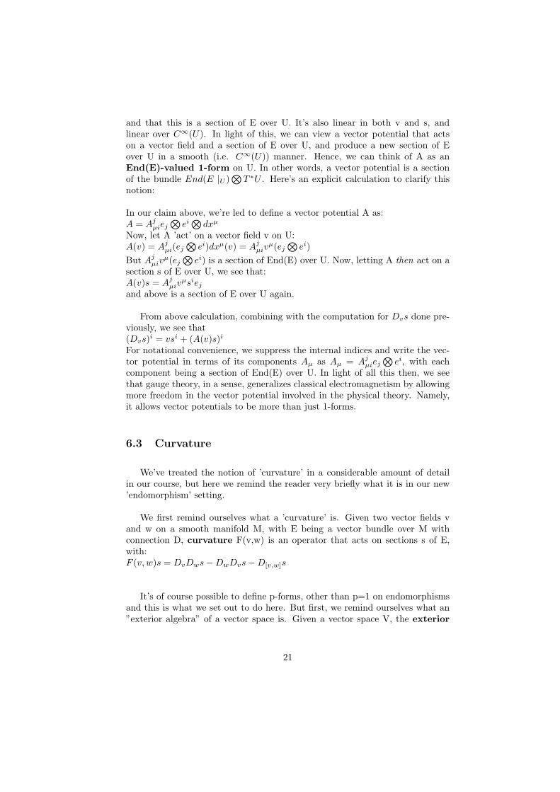
and that this is a section of E over U. It’s also linear in both v and s, andlinear over C∞(U). In light of this, we can view a vector potential that actson a vector field and a section of E over U, and produce a new section of Eover U in a smooth (i.e. C∞(U)) manner. Hence, we can think of A as anEnd(E)-valued 1-form on U. In other words, a vector potential is a sectionof the bundle End(E |U )

⊗T ∗U . Here’s an explicit calculation to clarify this

notion:

In our claim above, we’re led to define a vector potential A as:A = Aj

µiej

⊗ei

⊗dxµ

Now, let A ’act’ on a vector field v on U:A(v) = Aj

µi(ej

⊗ei)dxµ(v) = Aj

µivµ(ej

⊗ei)

But Ajµiv

µ(ej

⊗ei) is a section of End(E) over U. Now, letting A then act on a

section s of E over U, we see that:A(v)s = Aj

µivµsiej

and above is a section of E over U again.

From above calculation, combining with the computation for Dvs done pre-viously, we see that(Dvs)i = vsi + (A(v)s)i

For notational convenience, we suppress the internal indices and write the vec-tor potential in terms of its components Aµ as Aµ = Aj

µiej

⊗ei, with each

component being a section of End(E) over U. In light of all this then, we seethat gauge theory, in a sense, generalizes classical electromagnetism by allowingmore freedom in the vector potential involved in the physical theory. Namely,it allows vector potentials to be more than just 1-forms.

6.3 Curvature

We’ve treated the notion of ’curvature’ in a considerable amount of detailin our course, but here we remind the reader very briefly what it is in our new’endomorphism’ setting.

We first remind ourselves what a ’curvature’ is. Given two vector fields vand w on a smooth manifold M, with E being a vector bundle over M withconnection D, curvature F(v,w) is an operator that acts on sections s of E,with:F (v, w)s = DvDws−DwDvs−D[v,w]s

It’s of course possible to define p-forms, other than p=1 on endomorphismsand this is what we set out to do here. But first, we remind ourselves what an”exterior algebra” of a vector space is. Given a vector space V, the exterior

21

algebra over V, denoted∧V , is the algebra generated by V with the anti-

commutation relation v ∧ w = −w ∧ v, ∀v, w ∈ V.∧V is in fact an algebra as

can be easily seen, because in its definition, we see that we ”start” with a certainset (in fact a vector space V), then generate all possible elements through theformal products of the form v1∧...∧vp then take all possible linear combinationsof them, putting each of them in our

∧V , (where ∧ denotes the usual ’wedge

product’) with the constraint of the anti-commutation relation define above.With this definition, we construct, for a vector bundle E over M, an exterioralgebra bundle

∧E over M.

∧E over M is defined to have a total space⋃

p∈M

∧Ep, and the projection map π :

∧Ep → p. Though we won’t do this

here,∧E can be made into a manifold such that π :

∧E → M is a vector

bundle. In the specific instance of a tangent bundle TM, we form the dual(cotangent bundle) T ∗M , then we can form its exterior algebra bundle

∧T ∗M .

This special exterior algebra bundle is given its own name, form bundle. Adifferential form on a manifold M is then a section of the form bundle

∧T ∗M .

To derive Yang-Mills equations, we really need to do some ”calculus” withconnections and curvatures, as we’ll see soon. Towards that end, we defineEnd(E)-valued differential forms. We’ve already defined 1-forms of thistype and here we generalize the notion to higher degree forms. These are thesections of the bundle End(E)

⊗ ∧T ∗M , or its restriction to some open set

in M. Furthermore, given a vector bundle E over a smooth manifold M witha connection D, we define E-valued p-form to be a section of E

⊗ ∧pT ∗M .

Then an E-valued 0-form is just a section of E as we see. Last but not least, wecan define exterior covariant derivative dD of E-valued differential forms.For an E-valued 0-form (i.e. section) of E, we define it to be

dDs(v) = Dvs,∀v ∈ V ect(M)Note that this is a generalization of the well-known formula df(v) = v(f). In

local coordinates xµ on an open subset U ⊆ M, we have: dDs = Dµs⊗dxµ. Wecan now define the same notion on arbitrary E-valued differential forms. Let sbe a section of E and ω be an ordinary differential form on M. Then we defineit as:

dD(s⊗ ω) ≡ dDs ∧ ω + s⊗ dωMore importantly, if ω and µ are ordinary differential forms, then(T ⊗ ω) ∧ (s⊗ µ) = T (s)⊗ (ω ∧ µ).

7 The Yang-Mills Equation

Recall from our course work, that one of the two Maxwell’s equations (in dif-ferential forms setting) was just the result of the Bianchi identity. In thissection, we show what Yang-Mills equations are, and how they can be derivedfrom generalizing the Maxwell’s equations. In addition, we derive Yang-Millsequations from two different perspectives. One will be by considering fields inspace directly, the second approach will be a Lagrangian formulation.

22

7.1 The Hodge Star Operator and Maxwell’s Equations

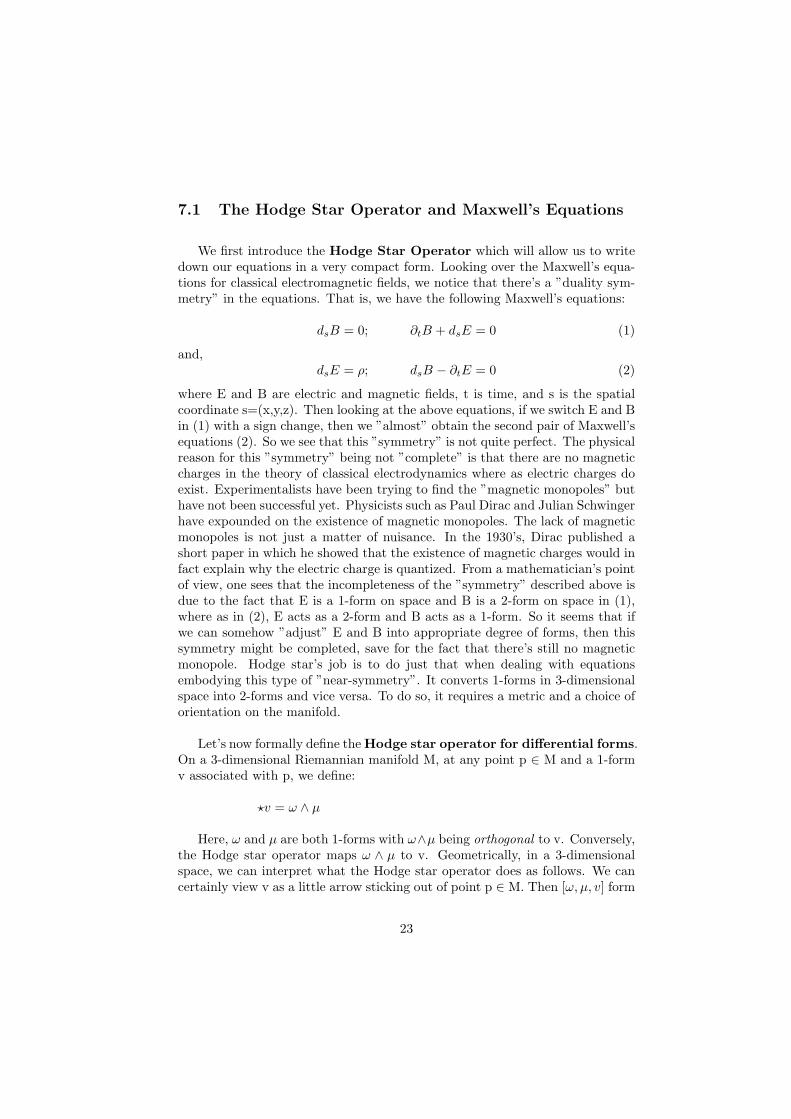
We first introduce the Hodge Star Operator which will allow us to writedown our equations in a very compact form. Looking over the Maxwell’s equa-tions for classical electromagnetic fields, we notice that there’s a ”duality sym-metry” in the equations. That is, we have the following Maxwell’s equations:

dsB = 0; ∂tB + dsE = 0 (1)

and,dsE = ρ; dsB − ∂tE = 0 (2)

where E and B are electric and magnetic fields, t is time, and s is the spatialcoordinate s=(x,y,z). Then looking at the above equations, if we switch E and Bin (1) with a sign change, then we ”almost” obtain the second pair of Maxwell’sequations (2). So we see that this ”symmetry” is not quite perfect. The physicalreason for this ”symmetry” being not ”complete” is that there are no magneticcharges in the theory of classical electrodynamics where as electric charges doexist. Experimentalists have been trying to find the ”magnetic monopoles” buthave not been successful yet. Physicists such as Paul Dirac and Julian Schwingerhave expounded on the existence of magnetic monopoles. The lack of magneticmonopoles is not just a matter of nuisance. In the 1930’s, Dirac published ashort paper in which he showed that the existence of magnetic charges would infact explain why the electric charge is quantized. From a mathematician’s pointof view, one sees that the incompleteness of the ”symmetry” described above isdue to the fact that E is a 1-form on space and B is a 2-form on space in (1),where as in (2), E acts as a 2-form and B acts as a 1-form. So it seems that ifwe can somehow ”adjust” E and B into appropriate degree of forms, then thissymmetry might be completed, save for the fact that there’s still no magneticmonopole. Hodge star’s job is to do just that when dealing with equationsembodying this type of ”near-symmetry”. It converts 1-forms in 3-dimensionalspace into 2-forms and vice versa. To do so, it requires a metric and a choice oforientation on the manifold.

Let’s now formally define the Hodge star operator for differential forms.On a 3-dimensional Riemannian manifold M, at any point p ∈ M and a 1-formv associated with p, we define:

?v = ω ∧ µ

Here, ω and µ are both 1-forms with ω∧µ being orthogonal to v. Conversely,the Hodge star operator maps ω ∧ µ to v. Geometrically, in a 3-dimensionalspace, we can interpret what the Hodge star operator does as follows. We cancertainly view v as a little arrow sticking out of point p ∈ M. Then [ω, µ, v] form

23

a basis of the 3-dimensional space with ω ∧ µ representing the area element ofthe parallelogram spanned by ω and µ, with v being orthogonal to the plane ofthe parallelogram.

We can generalize the construction of the Hodge star operator to n-dimensionsas follows:

? : p-forms → (n-p)-formsand it acts in a linear manner. It takes each ”p-dimensional area element” to anorthogonal ”(n-p)-dimensional area element”. To make this precise, we need aninner product of differential forms. So let’s do that. Let M be an n-dimensionaloriented semi-Riemannian manifold. We define an inner product of two p-forms ω and µ on M to be < ω, µ > as a function on M. With this notion of innerproduct, we then define the Hodge star operator ? : Ωp(M) → Ωn−p(M) asa unique linear map such that ∀µ, ν ∈ Ωp(M)

?(ω ∧ µ) ≡ (ω ∧ ?µ) =< ω, µ > volwhere Ωp(M) is the set of all p-forms on M and vol is the volume form associatedwith the metric on M. For example, vol at a point ∈ M is just volp = e1∧ ...∧en,where [e1, ..., en] is an oriented orthogonal basis of cotangent vectors at p. Notethat ω ∧ ?µ is an n-form because ?µ is an (n-p)-form and ω is a p-form. We saythat ?µ is a dual of µ.

Now that we’ve defined the Hodge star operator, what we want to do is getfamiliar with using it explicitly in computations involving differential forms (andlater on, involving vector bundles). By working out some explicit examples, we’lltry to convince ourselves that the Hodge star operator is indeed well-defined,and also get some perspectives on some of its important properties.

First, we state an equivalent definition of Hodge star operator that willbe computationally more useful. Let [e1, ..., en] denote a positively-orientedorthonormal basis of 1-forms on some chart of semi-Riemannian manifold M.Hence < eµ, eν > = 0 if and only if µ 6= ν, and < eµ, eµ > = ε(µ), whereε(µ) = ±1 with the sign depending on the chosen orientation. We claim thatfor any distinct set of indices 1 ≤ i1..., ip ≤ n:

?(ei1 ∧ ... ∧ eip) = ±eip+1 ∧ ... ∧ ein

where ip+1, ..., in = 1, ...n − i1, ..., ipWhich sign (either + or -) is assigned above is determined by:

sign(i1, ..., in)ε(i1)...ε(ip)where sign(i1, ..., in) denotes permutation that takes (1,...,n) to (i1, ..., in). Weclaim that this working definition of Hodge star is equivalent to the one givenpreviously, though we won’t prove the equivalence here.

The definition given above seems even more complicated than the originaldefinition of Hodge star, and in fact, it’s probably correct to say so. But fromabove definition, we can deduce the following very nice properties for 1-formsdx, dy, and dz in R3, taking the standard Euclidean metric and orientation:

24

?dx = dy ∧ dz, ? dy = dz ∧ dx, ? dz = dx ∧ dy (3)

And from above, we can further deduce the following, since Hodge star wasdefined to be an inverse of itself:

?(dx ∧ dy) = dz, ? (dz ∧ dx) = dy, ? (dy ∧ dz) = dx (4)

For any 0-form 1 and volume form dx∧dy∧dz, we have the following properties:

?1 = dx ∧ dy ∧ dz, ? (dx ∧ dy ∧ dz) = 1 (5)

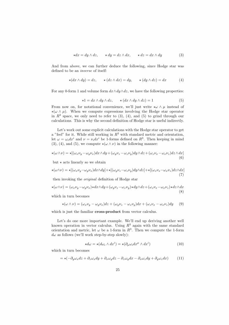
From now on, for notational convenience, we’ll just write ?ω ∧ µ instead of?(ω ∧ µ). When we compute expressions involving the Hodge star operatorin R3 space, we only need to refer to (3), (4), and (5) to grind through ourcalculations. This is why the second definition of Hodge star is useful indirectly.

Let’s work out some explicit calculations with the Hodge star operator to geta ”feel” for it. While still working in R3 with standard metric and orientation,let ω = ωidx

i and ν = νidxi be 1-forms defined on R3. Then keeping in mind

(3), (4), and (5), we compute ?(ω ∧ ν) in the following manner:

?(ω∧ν) = ?[(ωxνy−ωyνx)dx∧dy+(ωyνz−ωzνy)dy∧dz+(ωzνx−ωxνz)dz∧dx](6)

but ? acts linearly so we obtain

?(ω∧ν) = ?[(ωxνy−ωyνx)dx∧dy]+?[(ωyνz−ωzνy)dy∧dz]+?[(ωzνx−ωxνz)dz∧dx](7)

then invoking the original definition of Hodge star

?(ω∧ν) = (ωxνy−ωyνx)?dx∧dy+(ωyνz−ωzνy)?dy∧dz+(ωzνx−ωxνz)?dz∧dx(8)

which in turn becomes

?(ω ∧ ν) = (ωxνy − ωyνx)dz + (ωyνz − ωzνy)dx+ (ωzνx − ωxνz)dy (9)

which is just the familiar cross-product from vector calculus.

Let’s do one more important example. We’ll end up deriving another wellknown operation in vector calculus. Using R3 again with the same standardorientation and metric, let ω be a 1-form in R3. Then we compute the 1-formdω as follows (we’ll work step-by-step slowly):

?dω = ?(dωi ∧ dxi) = ?(∂µωidxµ ∧ dxi) (10)

which in turn becomes

= ?(−∂yωxdz + ∂zωxdy + ∂xωydz − ∂zωydx− ∂xωzdy + ∂yωzdx) (11)

25

= ?[(∂xωy − ∂yωx)dz + (∂zωx − ∂xωz)dy + (∂yωz − ∂zωy)dx] (12)

then using the linearity of ?,

= (∂xωy − ∂yωx) ? dz + (∂zωx − ∂xωz) ? dy + (∂yωz − ∂zωy) ? dz (13)

Then recalling (3) we have,

?dω = (∂xωy−∂yωx)dy∧dz+(∂zωx−∂xωz)dz∧dx+(∂yωz−∂zωy)dx∧dy (14)

which is just the curl of ω in vector calculus. In a similar manner, a computationof above type will prove that ?d ? ω is the divergence of ω.

Above lengthy computations are not in vain, for we can now use them toreduce Maxwell’s equations (1) and (2) down to the following:

dF = 0, ? d ? F = J (15)

where J is the electric current, and F is the electromagnetic field. So F encodesthe information about both the electric field E and the magnetic field B.

7.2 Derivation of the Yang-Mills Equation via field-theoreticmethod

In the previous section, we managed to reduce the Maxwell’s equations to amore compact version by using the Hodge star operator defined on differentialforms. We noted that F is the electromagnetic field that encodes both theelectric E and magnetic B fields. Then we can ’separate’ F into its magneticand electric parts on Minkowski spacetime

F = B + E ∧ dt (16)

Here, B and E are time-dependent 2-forms and 1-forms on space respectively.In certain physical situations, we can write the entire electromagnetic field F asan exterior derivative of some vector potential A, as noted previously,

F = dA (17)

Then we note that since d(dV)=0 for any vector potential V, that in fact thefirst of Maxwell’s equation (16) follows directly from this general fact aboutdifferential forms without recourse to any physical reasoning embodied in elec-tromagnetic fields. We remember, from our course, that this gives rise to thewell known Bianchi identity:

dDF = 0 (18)

where D is any well-defined connection.

26

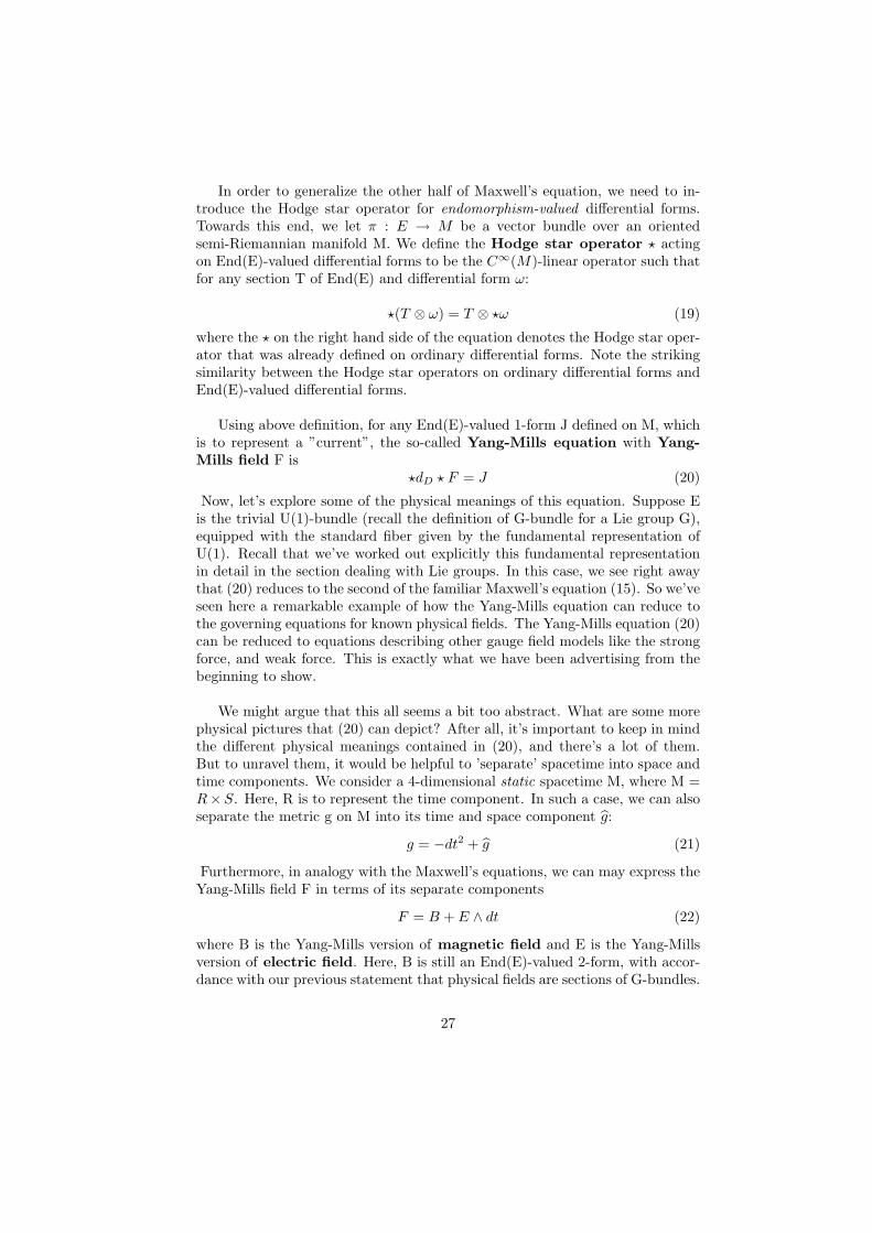
In order to generalize the other half of Maxwell’s equation, we need to in-troduce the Hodge star operator for endomorphism-valued differential forms.Towards this end, we let π : E → M be a vector bundle over an orientedsemi-Riemannian manifold M. We define the Hodge star operator ? actingon End(E)-valued differential forms to be the C∞(M)-linear operator such thatfor any section T of End(E) and differential form ω:

?(T ⊗ ω) = T ⊗ ?ω (19)

where the ? on the right hand side of the equation denotes the Hodge star oper-ator that was already defined on ordinary differential forms. Note the strikingsimilarity between the Hodge star operators on ordinary differential forms andEnd(E)-valued differential forms.

Using above definition, for any End(E)-valued 1-form J defined on M, whichis to represent a ”current”, the so-called Yang-Mills equation with Yang-Mills field F is

?dD ? F = J (20)

Now, let’s explore some of the physical meanings of this equation. Suppose Eis the trivial U(1)-bundle (recall the definition of G-bundle for a Lie group G),equipped with the standard fiber given by the fundamental representation ofU(1). Recall that we’ve worked out explicitly this fundamental representationin detail in the section dealing with Lie groups. In this case, we see right awaythat (20) reduces to the second of the familiar Maxwell’s equation (15). So we’veseen here a remarkable example of how the Yang-Mills equation can reduce tothe governing equations for known physical fields. The Yang-Mills equation (20)can be reduced to equations describing other gauge field models like the strongforce, and weak force. This is exactly what we have been advertising from thebeginning to show.

We might argue that this all seems a bit too abstract. What are some morephysical pictures that (20) can depict? After all, it’s important to keep in mindthe different physical meanings contained in (20), and there’s a lot of them.But to unravel them, it would be helpful to ’separate’ spacetime into space andtime components. We consider a 4-dimensional static spacetime M, where M =R×S. Here, R is to represent the time component. In such a case, we can alsoseparate the metric g on M into its time and space component g:

g = −dt2 + g (21)

Furthermore, in analogy with the Maxwell’s equations, we can may express theYang-Mills field F in terms of its separate components

F = B + E ∧ dt (22)

where B is the Yang-Mills version of magnetic field and E is the Yang-Millsversion of electric field. Here, B is still an End(E)-valued 2-form, with accor-dance with our previous statement that physical fields are sections of G-bundles.

27

E, in turn, is an End(E)-valued 1-form on space. We’ll stick with the conventionof denoting electric fields by E, and total space also by E. But keep in mindthat the ’E’ in ’End(E)’ is not the same as E representing the electric field! Wealso break down the current J into space and time components as

J = j − ρdt (23)

where j is an End(E)-valued 1-form on space and ρ is a section of End(E). Bothof them are time dependent functions. Remembering that D is a connectionand our definition of exterior covariant derivatives associated with connections,we can even decompose the exterior covariant derivative into its space and timeparts as follows:

dDω = dt ∧Dtω + dSω (24)

Where S denotes the spatial part (x,y,z) of course. Furthermore, if we recall theBianchi identity for connection D, we can separate that too into its respectivespace and time components using (24) to get

dDF = dSB + dt ∧ (DtB + dSE) = 0 (25)

But the two components are ’separate’, so above equality can only hold if boththe spatial and time components vanish

dSB = 0, DtB + dSE = 0 (26)

Now, using ?S to denote the Hodge star operator on End(E)-valued forms onS, we have, from (25) and (22),

?F = ?(B + E ∧ dt) = ?SE − ?SB ∧ dt (27)

Then combining (27) with (20), we obtain

?d ? F = −DtE − ?SdS ?S E ∧ dt+ ?SdS ?S B = j − ρdt (28)

Once again, as in (26), equating the space and time components, we see that

?SdS ?S E = ρ, −DtE + ?SdS ?S B = j (29)

We now show one of the important properties of Yang-Mills equations,gauge invariance. We’ve defined gauge invariance before, but recall that thismeans that if we have a connection D that satisfies the Yang-Mills equations,then any gauge transformation of D also satisfies it as well. This is not an easymatter and will take some work on our part. But here it goes.

7.3 Gauge Invariance of Yang-Mills Equation

28

As above, let D be a connection on the Yang-Mills electric field E, which isan End(E)-valued 1-form on space. We let g be a gauge transformation whichwas defined in the early part of our program. Furthermore, let D’ denote agauge transformation of D by g, where

D′vs = gDv(g−1s) (30)

with s being a section and v a vector field. We’ve defined what a curvature ofconnections is in the previous section. Recalling the definition, let F denote thecurvature of D and let F’ denote the curvature of D’. Then we have by definitionof curvature,

F ′(u, v)s = D′uD

′vs−D′

vD′us−D′

[u,v](g−1s) (31)

then substituting (30) into (31), we obtain

F ′(u, v)s = gDuDv(g−1s)− gDvDu(g−1s)− gD′[u,v](g

−1s) (32)

but this is just the definition of curvature on g−1s acted on by g,

F ′(u, v)s = gF (u, v)(g−1s) (33)

We denote this as F ′ = gFg−1 to be economical with our notations.

Now, we use our work above to show that indeed Yang-Mills equation isgauge invariant. Let F be the field satisfying the Yang-Mills equation (20). Withthe same notations as above, and using the definitions of Hodge star operatorgiven for End(E)-valued forms and curvature of connections given earlier, weget that

?dD ? F =12[Dµ, Fνλ]⊗ ?(dxµ ∧ ?(dxν ∧ dxλ)) (34)

This looks rather complicated but it follows strictly from the definitions if wejust substitute in. More specifically, Dµ is the covariant derivative on sectionsof E, andnot on sections of End(E). Then replacing D and F with the gaugetransformed connection D’ and curvature F’, we work out that

?dD′?F ′ =12[D′

µ, F′νλ]⊗?(dxµ∧?(dxν∧dxλ)) =

12[gDµg

−1, gFνλg−1]⊗?(dxµ∧?(dxν∧dxλ))

(35)where in the last part, we’ve simply invoked the definition of D’ and F’, both ofwhich were previously defined. We can simplify above expression even furtherby noting that

[gDµg−1, gFνλg

−1] = gDµg−1gFνλg

−1−gFνλg−1gDµg

−1 = gDµFνλg−1−gFνλDµg

−1 = g[Dµ, Fνλ]g−1

(36)Then (35) can be further simplified to

?dD′ ? F ′ =12g[Dµ, Fνλ]g−1 ⊗ ?(dxµ ∧ ?(dxν ∧ dxλ)) = g(?dD ? F )g−1 (37)

29

but g(?dD ? F )g−1 is just the gauge transformed current J’. Hence we haveshown that

?dD′ ? F ′ = J ′ (38)

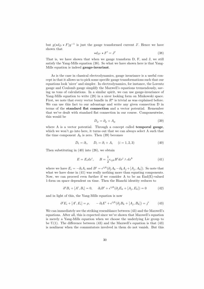
That is, we have shown that when we gauge transform D, F, and J, we stillsatisfy the Yang-Mills equation (38). So what we have shown here is that Yang-Mills equation is indeed gauge-invariant.

As is the case in classical electrodynamics, gauge invariance is a useful con-cept in that it allows us to pick some specific gauge transformations such that ourequations look ’nicer’ and simpler. In electrodynamics, for instance, the Lorentzgauge and Coulomb gauge simplify the Maxwell’s equations tremendously, sav-ing us tons of calculations. In a similar spirit, we can use gauge-invariance ofYang-Mills equation to write (28) in a nicer looking form on Minkowski space.First, we note that every vector bundle in Rn is trivial as was explained before.We can use this fact to our advantage and write any given connection D interms of the standard flat connection and a vector potential. Rememberthat we’ve dealt with standard flat connection in our course. Componentwise,this would be

Dµ = ∂µ +Aµ (39)

where A is a vector potential. Through a concept called temporal gauge,which we won’t go into here, it turns out that we can always select A such thatthe time component A0 is zero. Then (39) becomes

Dt = ∂t, Di = ∂i +Ai (i = 1, 2, 3) (40)

Then substituting in (40) into (26), we obtain

E = Eidxi, B =

12εijkB

idxj ∧ dxk (41)

where we have Ei = −∂tAi and Bi = εijk(∂jAk−∂kAj +[Aj , Ak]). So note thatwhat we have done in (41) was really nothing more than equating components.Now, we can proceed even further if we consider A to be an End(E)-valued1-form on space dependent on time. Then the Bianchi identity reduces to

∂iBi + [Ai, Bi] = 0, ∂tBi + εijk(∂jEk + [Aj , Ek]) = 0 (42)

and in light of this, the Yang-Mills equation is now

∂iEi + [Ai, Ei] = ρ, − ∂tEi + εijk(∂jBk + [Aj , Bk]) = ji (43)

We can immediately see the striking resemblance between (43) and the Maxwell’sequations. After all, this is expected since we’ve shown that Maxwell’s equationis merely a Yang-Mills equation when we choose the underlying Lie group tobe U(1). The difference between (43) and the Maxwell’s equation is that (43)is nonlinear when the commutators involved in them do not vanish. But this

30

occurs if and only if the underlying gauge group on which the Yang-Mills equa-tion (43) is based on is nonabelian. Recall that at the very beginning of ourprogram, when we first introduced the notion of Lie groups, we claimed thatthe nonabelian nature of the Lie group is intimately linked with the Yang-Millsequation becoming nonlinear. We see right here that indeed this is the case.

7.4 Derivation of Yang-Mills Equation via a Lagrangianformulation

Here we derive Yang-Mills equation through its Lagrangian, rather thanusing vector fields as we have previously. This method will reveal the symmetriesand several important properties of the equation more vividly. The Lagrangianformulation also helps us to ”quantize” fields, which is the basis of quantumfield theory.

We first ask ourselves where we should start. We start by noticing that theYang-Mills equation is founded upon its underlying vector bundle. Namely, letE be a vector bundle over a semi-Riemannian oriented n-dimensional manifoldM. Now, we’ll show that the Yang-Mills Lagrangian is an n-form that’s to beintegrated over M to get its associated action.

Towards formulating the Yang-Mills Lagrangian, it turns out to be necessaryto define the trace of an End(E)-valued form. We can define this notion inanalogy with the trace of a square matrix. Note that V is a vector space, so wecan select a basis for it and write elements of End(V) as matrices and defineour desired trace to be the trace on these matrices. This, however, turns outto be unnecessary because our trace turns out to be invariant under change ofbasis. We have shown previously that End(V) is isomorphic to V

⊗V ∗, and

this isomorphism is independent of choice of basis. Then we can define thefollowing linear map

tr : End(V ) → R, wheretr(v ⊗ f) → f(v) (44)

Let’s pick some basis ei of V and let ej be a dual basis of V ∗. Then pickT ∈ End(V ). Note that we can express T = T i

j ei ⊗ ej as shown when weintroduced the notion of endomorphisms in the previous section. Then we have

tr(T ) = T ij e

j(ei) = T ij δ

ji = T i

i (45)

which is the sum of the diagonal entries. So for a section T of End(E), we candefine tr(T) on the base space M such that for p ∈ M, tr(T)(p) = tr(T(p)).Note that T(p) is an endomorphism of the fiber Ep. Similarly, we define traceof an End(E)-valued form as follows:

tr(T ⊗ ω) = tr(T )ω (46)

where T is a section of End(E) and ω is a differential form.

31

Using above definition of trace, given a connection D on E, and a curvatureF of D, the Yang-Mills Lagrangian is defined to be

LY M =12tr(F ∧ ?F ) (47)

How we derive (47) from physical principles is quite a delicate matter that isbeyond the scope of this paper. To acquire the Yang-Mills action, we simplyneed to integrate (47) over M to get

SY M =12

∫M

tr(F ∧ ?F ) (48)

Then using the Euler-Lagrange equations, we obtain the Yang-Mills equationthat we got through the field-theoretic method in the previous section. Wechoose do not go into the actual derivation in this paper.

8 Epilogue

In this paper, we have tried to learn some basic facts about Lie groups, Liealgebras, vector bundles, and gauge theories while sampling different snippetsof physics whenever possible. We caution the reader, however, that each of theaforementioned areas constitutes a vast field of study in itself and that this paperserves no justice to any one of them. We hope that we have been successful inwetting the reader’s appetite in each of these different, yet linked areas andsparked his or her curiosity. For more information on these areas, we suggestthat the reader consult some of the materials listed as references in this paper.We have found the book ”Gauge fields, knots and gravity” by J. Baez and J. P.Muniain to be especially helpful in the development of this paper. As one cansee just from the amount of material we’ve presented here, gauge theory is quitea mature subject. Yet, it’s also important to point out that many parts of gaugetheory have yet to be developed, and its development is crucial to understandingsome of the most fundamental questions about nature, especially about gravity.The next revolution in physics will undoubtedly come in part from extension ofsome of the ideas presented here to the development of a coherent theory forgravity. None other than C. N. Yang himself has said it best and we end ourtreatise with a quote from him; ”Electromagnetism is, as we have seen, a gaugefield. That gravitation is a gauge field is universally accepted, although exactlyhow it is a gauge field is a matter still to be clarified.”

32

References

J. Baez, J. P. Muniain. Gauge Fields, Knots and Gravity.World Scientific. New Jersey, 1994.

C. N. Yang, R. L. Mills. Conservation of Isotopic Spin and Isotopic GaugeInvariance. Physical Review Vol. 96, No. 1, Oct. 1, 1954.

S. H. Friedberg, A. J. Insel, L. E. Spense. Linear Algebra, 3rd Ed.,Prentice Hall, New Jersey, 1997.

D. J. Griffiths. Introduction to Electrodynamics, 3rd Ed., Prentice Hall,New Jersey, 1999.

M. Peskin, D. Schroeder. An Introduction to Quantum Field Theory,Westview Press, 1995.

G. E. Simmons. Differential Equations with Applications and HistoricalNotes, 2nd Ed., McGraw-Hill, 1990.

33