a supply chain distribution network design model: an ...ceit.aut.ac.ir/~sa_hashemi/my...

ORIGINAL ARTICLE

A supply chain distribution network design model:An interactive fuzzy goal programming-basedsolution approach

Hasan Selim & Irem Ozkarahan

Received: 20 April 2006 /Accepted: 12 October 2006 /Published online: 12 December 2006# Springer-Verlag London Limited 2006

Abstract A supply chain (SC) distribution network designmodel is developed in this paper. The goal of the model isto select the optimum numbers, locations and capacitylevels of plants and warehouses to deliver products toretailers at the least cost while satisfying desired servicelevel to retailers. A maximal covering approach is used instatement of the service level. The model distinguishesitself from other models in this field in the modelingapproach used. Because of somewhat imprecise nature ofretailers’ demands and decision makers’ (DM) aspirationlevels for the goals, a fuzzy modeling approach is used.Additionally, a novel and generic interactive fuzzy goalprogramming (IFGP)-based solution approach is proposedto determine the preferred compromise solution. To explorethe viability of the proposed model and the solutionapproach, computational experiments are performed onrealistic scale case problems.

Keywords Supply chain . Distribution network design .

Interactive fuzzy goal programming .Maximal covering

AbbreviationsDM decision makerFGP fuzzy goal programmingFST fuzzy set theoryGP goal programmingIFGP interactive fuzzy goal programmingSC supply chainTCOST total costINV investmentTSERVL total service level

1 Introduction

The network design problem is one of the most compre-hensive strategic decision issues that need to be optimizedfor the long-term efficient operation of whole supply chain(SC). The decisions made for network design determine thenumber and locations of raw material suppliers, manufac-turing plants, intermediate warehouses and distributioncenters as well as select the distribution channel fromsuppliers to customers and identify the transportationvolume among distributed facilities for an extended timehorizon. Effective design and management of SC networksassists in production and delivery of a variety of products atlow cost, high quality, and short lead times. It is obviousthat an effective SC network structure is crucial in gaining acompetitive operational performance.

To cope with the complexity of the SC network designproblem, the network has been divided into several stagesin many previous studies. The number of stages isdetermined based on the tradeoffs between fragmentednetwork problem complexity and the network integrality[1]. For the SC network design problem, Jang et al. [2]decompose the entire network into three sub-networks,inbound network, distribution network and outboundnetwork.

A common objective in designing a distribution networkis to determine the least cost system design such that theretailers’ demand is satisfied without exceeding the capac-ities of the warehouses and plants. This usually involvesmaking tradeoffs inherent among the cost components ofthe system that include cost of opening and operating theplants and warehouses and the inbound and outboundtransportation costs.

There are two key decisions when designing a distribu-tion network [3]: 1) Will products be delivered to thecustomer location or picked up from a pre-ordained site? 2)Will products flow through an intermediary? Based on the

Int J Adv Manuf Technol (2008) 36:401–418DOI 10.1007/s00170-006-0842-6

H. Selim (*) : I. OzkarahanDepartment of Industrial Engineering, Dokuz Eylul University,35100 Izmir, Turkeye-mail: [email protected]

I. Ozkarahane-mail: [email protected]

choices for the two decisions, there are various types ofdistribution network designs that may be used to moveproducts from manufacturing plants to customer. Thereaders may refer to Chopra and Meindl [3] for the detaileddescription of each distribution option and the discussionon its strengths and weaknesses.

In this paper, we deal with a SC distribution networkcomprised of a set of manufacturing plants, warehouses andretailers. The network is illustrated in Fig. 1.

In the design option considered, inventory is storedlocally at retail stores and distributor warehouses. The mainadvantage of such a network structure is that it can lowerthe delivery cost and provide a faster response than othernetworks. The major disadvantage is the increased inven-tory and facility costs. As emphasized by Chopra andMeindl [3], such a network is best suited for fast-movingitems where customers value the rapid response.

Cost or profit-based optimization is the most widelyused method for SC distribution network design problems.However, more customer oriented approaches are requiredin order to provide a sustainable competitive advantage intoday’s business environment. Nowadays, there is a trend toconsider customer service level as more critical. Customerservice level can be measured by various measures such ascustomer response time, consistency of order cycle time,accuracy of order fulfillment rate, delivery lead time,flexibility in order quantity.

In this paper, we develop a multiobjective SC distribu-tion network design model. The goal is to select theoptimum numbers, locations and capacity levels of plantsand warehouses to deliver the products to the retailers at the

least cost while satisfying the desired service level to theretailers. Since the maximal covering approach [4] hasproved to be one of the most useful facility location modelsfrom both theoretical and practical points of view, we use itin statement of the service level. In the proposed model, acoverage function which may differ among the retailersaccording to their service standard request is defined foreach retailer.

Much of the decision making in the real world takesplace in an environment in which the goals, the constraints,and the consequences of the possible actions are not knownprecisely. As in the same manner, SCs operate in asomehow uncertain environment. Uncertainty may beassociated with target values of objectives, external supplyand customer demand etc. Supply chain distributionnetwork design models developed so far either ignoreduncertainty or consider it approximately through the use ofprobability concepts. However, when there is lack ofevidence available or lack of certainty in evidence, thestandard probabilistic reasoning methods are not appropri-ate. In this case, uncertain parameters can be specifiedbased on the experience and managerial subjective judg-ment. Fuzzy set theory (FST) [5] provides the appropriateframework to describe and treat uncertainty [6]. In decisionsciences, fuzzy sets have had a great impact in preferencemodeling and multi-criteria evaluation and have helpedbringing optimization techniques closer to the users needs.

As emphasized previously, SC distribution networkdesign problem is a strategic decision problem, theoptimization of which is crucial for the long-term efficientoperation of whole SC. The decisions to be made have

Fig. 1 Structure of the SCdistribution network

402 Int J Adv Manuf Technol (2008) 36:401–418

long-lasting effects and are costly, or sometimes impossibleto reverse. Because data are often incomplete and impre-cise, SC distribution network design decisions generally useforecasts based on aggregated data. As the environment orsystem changes, such impreciseness also propagates andcan exert serious effects on the operation and managementof the system. Another source of impreciseness may be dueto vagueness in DMs’ interpretation or intent. This situationoccurs when exactness is not required or is not possible tospecify, or when exactness would unnecessarily limitoptions. As stated by Reznik and Pham [7], exact or crispmodels when used in such cases would not be able tofaithfully simulate the richness and subtlety of the real workspace. Furthermore, in the worst case, misleading orincorrect outcomes may result. Thus, there is a need toarticulate the problems arising from such imprecisenesswith the view to construct appropriate models for theirrepresentation, as well as suitable methods for processingand manipulating them within the environment. Consider-ing this need, in this study, we use FST in handling SCdistribution network design problem. More specifically, twokind of impreciseness that may be faced in the problem,i.e., imprecision in retailers’ demand and DMs’ aspirationlevels for the goals, are treated. Additionally, to providethe DMs with a flexible and robust multi-objectivedecision making technique, we propose a novel andgeneric interactive fuzzy goal programming (IFGP)-basedsolution approach. Through the solution approach, DMsdetermine the preferred compromise solution.

The paper is further organized as follows: A review ofthe related literature is presented in the next section.Thereafter, basic concepts and the framework of fuzzy goalprogramming (FGP), and the proposed IFGP-based solu-tion approach are presented in Sects. 3 and 4, respectively.Section 5 is devoted to the presentation of the crispformulation of the proposed SC distribution network designmodel. Computational experiments are presented in Sect. 6.Finally, conclusions are presented in Sect. 7.

2 Literature review

Numerous researchers have extensively studied facility anddemand allocation problems. Interested readers may refer todetailed survey results, e.g., Francis et al. [8], Aikens [9],Brandeau and Chiu [10], Beamon [11], Avella et al. [12]and Pontrandolfo and Okogbaa [13].

Beamon [11] provides a focused review of literature inthe area of multi-stage SC design and analysis and classifythe models in the area into four categories: deterministicanalytic models, stochastic analytic models, economicmodels, and simulation models. Avella et al. [12] presenttheir views on the state of the art and the future trends in

location analysis. Pontrandolfo and Okogbaa [13] reviewthe literature on the configuration as well as the coordina-tion of the network of global facilities problems. Theydefine a framework that systematically addresses the globalmanufacturing planning problem by identifying and classi-fying the variables involved therein.

The last decades of the twentieth century witnessed aconsiderable expansion of SCs into international locations.This growth in globalization, and the additional manage-ment challenges it brings, has motivated both practitionerand academic interest in global SC management [14]. Inthis paper, we do not consider the global issues in theproposed model.

After mentioning some important reviews on SCnetwork design problem, we present a review of the severalrelevant papers in the following. In our review, we focusespecially on the papers that develop or consider lineardeterministic SC network design models.

Geoffrion and Graves [15] presents a new method for thesolution of the problem addresses the optimal location ofdistribution centers between plants and customers. Theydevelop an algorithm based on Benders’ decomposition forsolving multi-commodity distribution network design prob-lem. Brown et al. [16] present a mixed integer model for amulti-commodity production-distribution system. The ob-jective of the model is to minimize the variable productionand shipping cost, fixed cost of equipment assignment andplant operations. They apply to the model a primaldecomposition technique similar to Geoffrion and Graves’[15] algorithm. Cohen and Lee [17] present a strategicmodel structure and a hierarchical decomposition approach.The scope of their work is to analyze interactions betweenfunctions in a complete SC network. To model theseinteractions they consider four sub modules where eachrepresents a part of the overall SC: (1) material control, (2)production control, (3) finished goods stockpile, and (4)distribution network control.

Pirkul and Jayaraman [18] consider a tri-echelon, multi-commodity system concerning production, distribution andtransportation planning. The authors use a Lagrangeanrelaxation-based heuristic to provide effective an effectivefeasible solution. Jayaraman [19] studies the capacitatedwarehouse location problem that involves locating a givennumber of warehouses to satisfy customer demands fordifferent products. Pirkul and Jayaraman [1] extend theprevious problem by considering locating also a givennumber of plants. They present a model for multi-commodity, multi-plant, capacitated facility location prob-lem, and develop a Lagrangean-based heuristic solutionprocedure. Dogan and Goetschalckx [20] develop a mixedinteger linear programming model for the integrated designof multi-period production-distribution systems. Theirpaper contributes to the literature by developing an

Int J Adv Manuf Technol (2008) 36:401–418 403

integrated design methodology for strategic production anddistribution systems using primal decomposition theory. Italso provides an acceleration methodology for solving theproblem. Tragantalerngsak et al. [21] consider a two-echelon facility location problem in which the facilities inthe first echelon are incapacitated and the facilities in thesecond echelon are capacitated. The goal in their model isto determine the number and locations of facilities in bothechelons in order to satisfy customer demand of theproduct. They develop a Lagrangean relaxation-basedbranch and bound algorithm to solve the problem. Lee etal. [22] develop a multi-product mixed integer nonlinearprogramming model to develop a capacity expansion of anintegrated production and distribution system. The systemcomprises the multi-site batch plants and warehouses.Melachrinodis and Min [23] design a multi-objective,multi-period mixed integer programming model that deter-mine the optimal relocation site and phase out schedule of acombined manufacturing and distribution facility from SCperspectives. Their research differentiates from the litera-ture by considering both dynamic aspects and multi-echelon network design. Sabri and Beamon [24] developa SC model that considers simultaneous strategic andoperational SC planning. The main contribution of thework is the incorporation of production, delivery, anddemand uncertainty into one model. Pirkul and Jayaraman[25] present an integrated logistic model, and develop anefficient solution procedure for multi-commodity produc-tion-distribution problem.

Tsiakis et al. [26] develop a strategic planning model forSC networks. The paper takes into consideration flexibleproduction facilities in which a number of products areproduced making use of shared resources, the economies ofscale in transportation, and uncertainty in product demand.Jang et al. [2] propose a supply network with a global billof material. They model design and planning problems of asupply network in a single combined system. Talluri andBaker [27] propose a multi-phase mathematical program-ming approach for effective SC network design. Cakravastiaet al. [28] develop a mixed integer programming model ofthe supplier (any manufacturer playing a lower-levelsupporting role) selection process in designing a SCnetwork. The assumed objective of the SC is to minimizethe level of customer dissatisfaction, which is evaluated bytwo criteria: (i) price and (ii) delivery lead time.

More recently, Beamon and Fernandes [29] study aclosed-loop SC in which manufacturers produce newproducts and remanufacture used products. The multi-period integer programming model uses the present worthmethod to jointly analyze investment and operational costs.Yeh [30] presents a hybrid heuristic algorithm to solve themulti-stage SC network design problem. The algorithmcombines a greedy method, the linear programming

technique and three local search methods, the pair-wiseexchange procedure, the insert procedure and the removeprocedure. Eskigun et al. [31] deal with the design of a SCdistribution network considering lead time, location ofdistribution facilities and choice of transportation mode.They present a Lagrangian heuristic that gives goodsolution quality in reasonable computational time. In arecent paper, Amiri [32] addresses the distribution networkdesign problem in a SC system. The author develops amixed integer programming model and provides a heuristicsolution procedure.

The contribution of our current paper to the literature istwofold: First, a fuzzy multi-objective model has beendeveloped for SC distribution network design problem.Second, a novel and generic IFGP-based solution ap-proach is proposed to determine the preferred compromisesolution.

3 Fuzzy goal programming

Goal programming (GP) is one of the most powerful, multi-objective decision making approaches in practical decisionmaking. In a standard GP formulation, goals are definedprecisely. However, application of GP to the real life prob-lems may be faced with two important difficulties. One ofwhich is expressing the DMs’ vague goals mathematicallyand the second is the need to optimize all goals simulta-neously. In such situations, the use of FST comes in handy.

Applying FST into goal programming (GP) has theadvantage of allowing for the vague aspirations of a DM,which can then be qualified by some natural languageterms. The FST in GP was first considered by Narasimhan[33]. Goal programming in fuzzy environment is furtherdeveloped by Hannan [34], Ignizio [35], Narasimhan andRubin [36], Tiwari et al. [37, 38] and others.

A fuzzy set A can be characterized by a membershipfunction, usually denoted by μ, which assigns to eachobject of a domain its grade of membership in A. Thenearer the value of membership function to unity, the higherthe grade of membership of element or object in a fuzzy setA. Various types of membership functions can be used torepresent the fuzzy set.

A typical FGP problem formulation can be stated asfollows:

Find xi; i ¼ 1; :::; n

Zm xið Þ � Zm m ¼ 1; :::; M

Zk xið Þ � Zk k ¼ M þ 1; :::; K

gj xið Þ � bj j ¼ 1; :::; J

xi � 0 i ¼ 1; :::; n

9>>>>>>=>>>>>>;

ð1Þ


where, Zm(xi) is the mth goal constraint, Zk (xi) is the kthgoal constraint, Zm xið Þ is the target value of the mth goal,Zk xið Þ is the target value of the kth goal, gj (xi) is the jthinequality constraint and bj is the available resource ofinequality constraint j.

In formulation (1), the symbols “≺ and ≻” denote thefuzzified versions of “≤ and ≥” and can be read asapproximately less / greater than or equal to. These twotypes of linguistic terms have different meanings. Underapproximately less than or equal to situation, the goal m isallowed to be spread to the right-hand-side of Zm(Zm ¼ lmwhere lm denote the lower bound for the mth objective)with a certain range of rm(Zm þ rm ¼ um, where um denotethe upper bound for the mth objective). Similarly, withapproximately greater than or equal to, pk is the allowedleft side of Zk Zk � pk ¼ lk ; and Zk ¼ uk

� �.

As can be seen, GP and FGP have some similarities.Both of them need an aspiration level for each objective.These aspiration levels are determined by DMs. In additionto the aspiration levels of the goals, FGP needs max-minlimits (uk,lk) for each goal. While the DMs decide the max-min limits, the linear programming results are startingpoints and the intervals are covered by these results.Generally, the DMs find estimates of the upper (u) andlower (l) values for each goal using payoff table (seeTable 1). Therefore, the feasibility of each fuzzy goal isguaranteed.

Here, Zm(X) denotes the mth objective function, and X(m)

is the optimal solution of the mth single objective problem.Solving the problem with X(m) (m=1,..., M) for eachobjective, a payoff matrix with entries Zpm ¼ Zm X ðpÞ� �

, m,p=1,..., M can be formulated as presented in Table 1. Here,um ¼ max Z1m; Z2m; . . . ; ZMmð Þ and lm=Zmm, m=1,..., M.

After constructing fuzzified aspiration levels with respectto the linguistic terms of approximately less than or equalto, and approximately greater than or equal to, themembership functions can be developed for each goal.

Using Belman & Zadeh’s [39] min operator approach,one can obtain the feasible fuzzy solution set by theintersection of all membership functions representing thefuzzy goals. This solution set is then characterized by itsmembership μF(x) which is:

mF xð Þ ¼ mZ1 xð Þ \ mZ2 xð Þ:::: \ mZk xð Þ¼ min mZ1 xð Þ;mZ2 xð Þ; ::::;mZk xð Þ� � ð2Þ

Then the optimum decision can be determined to be themaximum degree of membership for the fuzzy decision:

maxx2F

mF xð Þ ¼ maxx2F

min mZ1 xð Þ;mZ2 xð Þ; :::; mZk xð Þ� � ð3Þ

By introducing the auxiliary variable λ, which is theoverall satisfactory level of compromise, formulation (2)

can be transformed to the following conventional linearprogramming problem [40]:

maximize 1

subject to

1 � μZk k ¼ 1; :::;K

gj xið Þ � bj i ¼ 1; :::; n; j ¼ 1; :::; J

xi � 0 i ¼ 1; :::; n

1 2 0; 1½ �:

9>>>>>>>>>=>>>>>>>>>;

ð4Þ

4 The proposed IFGP-based solution approach

By use of the interactive paradigm, interactive fuzzymultiobjective decision making approaches have beeninvestigated to improve the flexibility and robustness ofmultiobjective decision making techniques. They providelearning process about the system, whereby the DM canlearn to recognize good solutions and relative importance offactors in the system [41]. The main advantage ofinteractive approaches is that the DM controls the searchdirection during the solution procedure and, as a result, theefficient solution achieves his/her preferences [42]. Litera-ture in the class of fuzzy interactive programming includesWerners [43, 44], Leung [45], Fabian et al. [46], Sasaki etal. [47] and Baptistella and Ollero [48].

Belman and Zadeh’s [39] min operator focuses only onthe maximization of the minimum membership grade. It isnot a compensatory operator. That is, goals with a highdegree of membership are not traded off against goals witha low degree of membership. Therefore, some computa-tionally efficient compensatory operators (see [41]) can beused in setting the objective function in fuzzy programmingto investigate better results.

One criterion used to evaluate the performance ofcompensatory operators in fuzzy optimization is monoto-nicity. Among the compensatory operators which are wellsuited in solving multiobjective programming problems,Werners’ [49] ‘fuzzy and’ operator has an advantage ofbeing a strongly monotonically increasing function. That is,it is positively related with the compensation rate. Further-more, it is easy to handle, and has generated reasonableconsistent results in applications. For those reasons, weemploy Werners’s ‘fuzzy and’ operator in the proposedIFGP-based solution approach.

Table 1 The payoff table

Z1(X) Z2(X) ... ZM(X)

X (1) Z11 Z12 ... Z1MX (2) Z21 Z22 ... Z2M...

... ... ... ...X (M) ZM1 ZM2 ... ZMM


Werners [49] formulates the ‘fuzzy and’ operator asfollows:

μD xð Þ ¼ Max + minkμk xð Þð Þ þ 1� +ð Þ 1=Kð Þ

Xk

μk xð Þ( )

ð5Þwhere K is the total number of fuzzy objectives andconstraints, μk(x) is the membership function of fuzzy goalk, and + is the coefficient of compensation defined withinthe interval [0,1]. By adopting min operator into Eq. (5),the following linear programming problem can be formed:

maximize +1 þ 1� +ð Þ 1=Kð ÞXk

1 k

subject to μk xð Þ � 1 þ 1 k ; 8k 2 K; 8x 2 X

1 ; 1 k ; + 2 0; 1½ �:

9>>>=>>>;ð6Þ

In real life decision problems, the relative importance ofthe objectives assigned by the DMs may not be equal, andmay change over time. Different from ‘fuzzy and’ operator,the proposed IFGP approach consider the relative impor-tance of the objectives, and consequently provides a morerealistic structure.

To reflect the relative importance of λks to the objectivefunction, we develop and use a modified version of the‘fuzzy and’ operator in the proposed solution approach.More specifically, we use the following formulation:

maximize glþ 1� gð ÞPkwklk ð7Þ

subject to the constraints in formulation (6), wherePkwk ¼ 1.In order to determine the weights, there are some good

approaches in the literature, such as analytic hierarchyprocess, weighted least square method and the entropymethod etc. Also, there are some fuzzy approaches forfinding crisp weights in fuzzy environment. However,determination of the weights is not the focus of this study.

We think that the coefficient of compensation (γ) can betreated as the degree of willingness of the SC partners tosacrifice the aspiration levels for their goals to some extentin the short run to provide the loyalty of their partners and/or to strengthen their competitive position in the long run.We also think that the coefficient of compensation can bedetermined through a consensus decision making process.In this process, complete unanimity is not the goal - that israrely possible. However, it is possible for each SC memberto have had the opportunity to express their opinion, belistened to, and accept a group decision based on its logicand feasibility considering all relevant factors. This requiresthe mutual trust and respect of each member.

We assert that uncertainties of the input data and theDMs’ aspiration levels for the goals in multiobjective linearprogramming problems can be treated through the proposedIFGP-based solution approach, and consequently, thepreferred compromise solution can be determined. Beforeintroducing the proposed solution approach, we think thatpresentation of some definitions and theoretic explanationsrelated to the topic may be useful for clarity.

Definitions of the compromise solution and the preferredcompromise solution are presented in the following [42].

Fig. 2 Flowchart of the proposed IFGP-based solution approach

iLB iUB

ijm

ijdt

Fig. 3 Illustration of linear coverage function


Compromise solution: A feasible vector X* Z S is called acompromise solution of the problem iff X* Z E andZ X �ð Þ � ^X2SZ Xð Þ where Z(X) is the objective function, Sis the feasible region, $ stands for “minimum” and E is theset of efficient solutions.

This definition imposes two conditions on the solutionfor it to be a compromise solution. First, the solution shouldbe efficient. Second, the compromise solution is the closestsolution to the ideal one that maximizes the underlyingutility function of the DM. In real-world cases, knowledgeof the set of efficient solutions E is not always necessary.On the other hand, the DMs’ preferences are to beconsidered in determining the final compromise solution.

Preferred compromise solution: If the compromise solutionsatisfies the DMs’ preferences, then it is called the preferredcompromise solution.

The proposed IFGP-based solution approach can besummarized in the following steps:

– Step 1: Develop the conventional (crisp) linearprogramming formulation of the problem.

– Step 2: Obtain efficient extreme solutions (payoffvalues) used for constructing the membership functionsof the objectives. If the DM selects one of them as apreferred compromise solution go to Step 7. Otherwisego to Step 3.

– Step 3: Define the membership function of each fuzzyobjective using upper and lower bounds of theobjectives.

– Step 4: Considering the membership functions definedin Step 3 and γ (fix the value of γ to 1 in the firstiteration) develop the formulation of the problem usingproposed ‘modified fuzzy and’ operator.

– Step 5: Obtain a compromise solution and present thesolution to the DM. If the DM accepts it, go to Step 7.Otherwise, go to Step 6.

– Step 6: Ask the DM if he want to modify thecoefficient of compensation (γ), and membershipfunctions of the objectives, and go to Step 3. Actually,definition of a unique rule, e.g., selection of the initialvalue, change direction or rate of variation in each step,by which the value of γ is varied is difficult since itdepends on DMs’ preferences. For instance, if theproblem under concern is so sensitive to γ, the rate ofvariation should be sufficiently slow. When the DMtries to modify membership functions of the objectivesand constraints, only the following variations areacceptable [43]: a) the increase of lower bound (lk)for the maximization objectives, b) the decrease ofupper bound (um) for the minimization objective, c) the

Table 2 Formulation of theobjective functions

Table 3 Expected demand of the retailers

Demand for product I (ai l) Demand for product II (ai2)

992 408 556 831 352 229 282 894 976 880423 573 388 683 378 898 968 845 885 988659 873 467 653 649 844 960 935 847 629806 222 501 669 483 306 789 968 334 971107 377 777 701 709 845 195 610 776 743500 439 759 264 449 758 736 976 923 339741 783 516 507 455 508 198 496 927 811257 936 327 174 528 916 630 813 320 466956 317 664 878 484 171 955 424 658 720129 887 929 609 514 403 186 505 700 724

Table 4 Lower and upper bounds for the distance

Retailers Lower bound (LBi) Upper bound (UBi)

1–12 500 65013–27 600 75028–50 700 850


decrease of maximum tolerance (dj) is an acceptablemodification which can guarantee an efficient solutionin the recalculated compromise solution step. In orderto avoid the possibility of getting into infeasiblesolution sets because of excess increase of lk or excessdecrease of um, we should increase lk and decrease umas few requirements as possible in each iteration.

– Step 7: Stop.

The flow chart of these steps is shown in Fig. 2.

5 Crisp formulation of the proposed model

In this section, we present the crisp formulation of theproposed SC distribution network design model. The goalof the model is to select the optimum numbers, locationsand capacity levels of plants and warehouses to deliver theproducts to the retailers at the least cost while satisfying thedesired service level to the retailers. Maximal coveringapproach is used in statement of the service level, and acoverage function which may differ among the retailersaccording to their service standard request is defined foreach retailer. The proposed model distinguishes itself fromother models in this field in the modeling approach used.Because of somehow imprecise nature of retailers’ demandand DMs’ aspiration levels for the goals, fuzzy modelingapproach is used. Additionally, a novel and generic IFGP-based solution approach is proposed to determine thepreferred compromise solution.

The mathematical model is developed on the basis of thefollowing assumptions:

– The network considered encompasses a set of retailerswith known locations, and possible discrete set oflocation zones/sites where warehouses and plants arelocated.

– Different capacity levels are available to both thepotential plants and warehouses.

– The retailers have demand for a multitude of products,and the warehouses are responsible for right-timedelivery of a right amount of products.

– Decision makers of the plants, warehouses and retailersshare information and collaborate with each other todesign an effective distribution network.

– Decisions are made within a single period.

5.1 Notations and definitions

Definitions of sets, parameters and decision variables of theproposed model are presented in the following.

– Sets

I set of zones where retailers are located,J potential warehouse locations,K potential plant locations,L set of products,R set of capacity levels available for warehouses,H set of capacity levels available for plants.

– Parameters

Tjkl variable cost to transport one unit of productl from the plant in zone k to the warehouse inzone j

Cijl variable cost to transport one unit of productl from the warehouse in zone j to the retailer inzone i

fkh fixed portion of the operating cost of the plant inzone k with capacity level h

gjr fixed portion of the annual possession andoperating costs of the warehouse in zone j withcapacity level r

OPkh opening cost of the plant in zone k with capacitylevel h

OWjr opening cost of the warehouse in zone j withcapacity level r

ail demand for product l by the retailer in zone isl required throughput capacity of a warehouses for

product lWjr throughput capacity of the warehouse in zone j

with capacity level rql required production capacity of a plant for

product lDkh capacity of the plant in zone k with capacity level hdtij distance between zone i and zone j


TCOST INV TSERVL

TCOST 2,720,667 2,663,710 52,046INV 3,250,000 2,229,724 50,000TSERVL 3,250,000 2,994,668 61,532

Table 6 Lower and upper bounds for the objectives

Objectives Lower bound Upper bound

TCOST 2,720,667 3,250,000INV 2,229,724 2,994,668TSERVL 50,000 61,532

Table 7 Compromise solution results with min operator

γ λ TCOST INV TSERVL μTCOST μINV μTSERVL

1 0.5317 2,968,563 2,583,509 56,131 0.5317 0.5317 0.5317


mij coverage parameter that denotes the coverage levelof the retailer in zone i by the warehouse in zone j

LBi,UBi

the parameters that are used in defining thecoverage parameter of the retailer in zone i, LBi

and UBi denote lower and upper bound for thedistance, respectively (see Fig. 3).

– Decision variables

Yjkl amount of product l transported to the warehouse inzone j from the plant in zone k,

Xijl amount of product l transported to the retailer in zonei from the warehouse in zone j,

Zjr binary variable that indicates whether a warehousewith capacity level r is constructed in zone j,

Pkh binary variable that indicates whether a plant withcapacity level h is constructed in zone k.

5.2 The objective functions

Objective functions of the model are formulated as follows:As can be seen from Table 2, the first objective function

minimizes total cost made of: the transportation costs ofproducts from plants to warehouses and from warehouses toretailers, and the fixed costs associated with the plants andthe warehouses. While the second objective functionminimizes the investment in opening plants and ware-

houses, the third one maximizes the total service levelprovided to the retailers.

5.3 The constraints

The constraints of the proposed model and their definitionsare presented in the following.Xj

Xijl ¼ ail for all i 2 I and l 2 L; ð11Þ

Constraint set (11) ensures that all demand from retailersis satisfied by warehouses.Xi

Xl

slXijl �Xr

WjrZjr for all j 2 J ; ð12Þ

Constraint set (12) limits the distribution quantities thatare shipped from warehouses to retailers to the throughputlimits of warehouses.Xr

Zjr � 1 for all j 2 J ; ð13Þ

Constraint set (13) ensures that a warehouse can beassigned at most one capacity level.Xi

Xijl �Xk

Yjkl for all j 2 Jand l 2 L; ð14Þ

Constraint set (14) guarantees that all demand fromretailer in zone i for product l is balanced by the total units

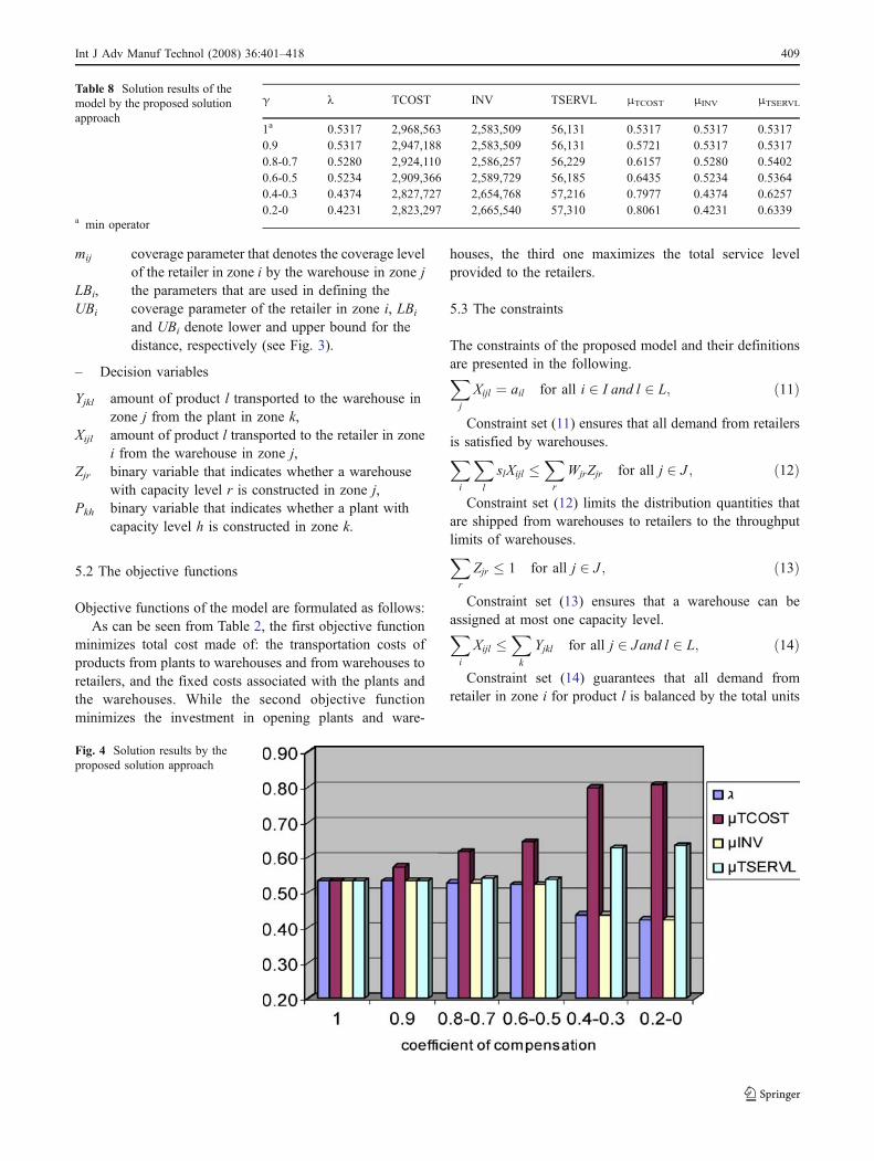
Table 8 Solution results of themodel by the proposed solutionapproach

a min operator


1a 0.5317 2,968,563 2,583,509 56,131 0.5317 0.5317 0.53170.9 0.5317 2,947,188 2,583,509 56,131 0.5721 0.5317 0.53170.8-0.7 0.5280 2,924,110 2,586,257 56,229 0.6157 0.5280 0.54020.6-0.5 0.5234 2,909,366 2,589,729 56,185 0.6435 0.5234 0.53640.4-0.3 0.4374 2,827,727 2,654,768 57,216 0.7977 0.4374 0.62570.2-0 0.4231 2,823,297 2,665,540 57,310 0.8061 0.4231 0.6339

Fig. 4 Solution results by theproposed solution approach


of product l available at warehouse in zone j that has beensupplied from open plants.Xj

Xl

qklYjkl �Xh

DkhPkh for all k 2 K; ð15Þ

Constraints in set (15) represent the capacity restrictionsof the plants in terms of their total shipments to thewarehouses.Xh

Pkh � 1 for all k 2 K; ð16Þ

Constraint set (16) ensures that a plant can be assignedat most one capacity level.

Zjr 2 0; 1f g for all j 2 J ; r 2 R;Pkh 2 0; 1f gfor all k 2 K; h 2 H

ð17Þ

Finally, constraint set (17) enforces the binary and non-negativity restrictions on the decision variables.

6 Computational experiments

6.1 The problem and parameter structuring

To explore the viability of the proposed model and theIFGP-based solution approach, computational experimentsare presented in this section. The experiments are classifiedinto two categories. Imprecision in the DMs’ aspirationlevels for the goals is treated in the first category, whileimprecision in both the retailers’ demand and DMs’aspiration levels for the goals is treated simultaneously inthe second category. Solutions of the proposed model are

performed using Werners’ (1988) ‘fuzzy and’ operator andthe proposed solution approach, and the results are com-pared.

A hypothetically constructed SC distribution networkdesign problem with 50 retailer zones, 20 potentialwarehouse sites and 15 potential plant sites is consideredin the computational experiments. It is assumed that twodifferent types of product are demanded by the retailers.Coordinates of the retailer zones, potential warehouses andplant sites are generated from a uniform distribution over asquare with side 3000. Euclidean distances are used indefining the coverage parameters. CPLEX 9.1 optimizationsoftware is used at the solution stage.

Before presenting the computational experiments, let usexplain the parameter structuring of the hypothetical SCdistribution network design problem under concern.

Expected demand of the retailers for two differentproducts is drawn from a uniform distribution between100 and 1000 as given in Table 3.

Five capacity levels are used for the capacities availableto both the potential plants and warehouses. The openingcost of the warehouse in zone j with capacity level 3 (OWj3)are drawn from a uniform distribution between 90,000 and120,000. The opening costs of the warehouses for the othercapacity levels are computed as follows: OWj1=0.75*OWj3,OWj2=0.85*OWj3, OWj4=1.15*OWj3, OWj5=1.25*OWj3.Cost coefficients of OPkh are computed in terms of thewarehouses costs as OPkh=4*OWkh. Fixed portion of theannual possession and operating costs of the warehouse inzone j with capacity level 3 (gj3) and the plant in zone kwith capacity level 3 (fk3) are drawn from a uniformdistribution between 18,000 and 25,000 and 75,000 and100,000, respectively. Fixed portion of the annual possessionand operating costs of warehouses and plants for the othercapacity levels are computed as follows: gj1=0.75*gj3, gj2=0.85*gj3, gj4=1.15*gj3, gj5=1.25*gj3 and fk1=0.75*fk3, fk2=0.85*fk3, fk4=1.15*fk3, fk5=1.25*fk3.

Required throughput capacity of a warehouse for productl and required production capacity of a plant for product l aregiven as follows: s1=1, s2=1 and q1=1, q2=2. The costcoefficients Cijl and Tjkl are computed as being proportionalto the Euclidean distance among the locations of warehousesand retailers, and plants and warehouses, respectively.

Table 9 Solution results obtained by the proposed solution approachin terms of utilization of the plants and warehouses

γ Utilization of the plants Utilization of the warehouses

Min Max Average Min Max Average

1 0.87 1 0.97 0.90 1.00 0.970.9 0.87 1 0.97 0.91 1.00 0.970.8-0.7 0.89 1 0.97 0.82 1.00 0.970.6-0.5 0.87 1 0.97 0.90 1.00 0.970.4-0.3 0.87 1 0.97 0.86 1.00 0.970.2-0 0.88 1 0.96 0.75 1.00 0.93

Table 10 Solution results of the model by Werners’ ‘fuzzy and’ operator


1 0.5317 2,968,563 2,583,509 56,131 0.5317 0.5317 0.53170.9 0.5317 2,947,407 2,583,509 56,135 0.5716 0.5317 0.53200.8-0.6 0.5280 2,924,274 2,586,257 56,233 0.6154 0.5280 0.54050.5 0.5234 2,909,366 2,589,729 56,185 0.6435 0.5234 0.53640.4-0.1 0.4448 2,879,877 2,649,159 58,338 0.6992 0.4448 0.72310 0.0000 2,879,877 2,649,159 58,338 0.6992 0.4448 0.7231


Specifically, Cijl and Tjkl are drawn from a uniformdistribution between 0.025*dtij and 0.035*dtij and 0.045*dtjkand 0.055*dtjk, respectively. The parameters that are used indefining the coverage parameter of retailer in zone i (LBi,UBi), are given in Table 4. Throughput limit of warehouse inzone j with capacity level r (Wjr) and capacity of the plant inzone k with capacity level h (Dkh) are taken as follows.

Wjr=4000, 6000, 8000, 10000, 12000, Dkh=15000,20000, 30000, 35000, 40000.

6.2 Implementation category I: treatment of fuzzyaspiration levels for the goals

In this category of experiments, the imprecision in goalachievement is allowed through the specification of aninterval of acceptable achievement rather than a crispvalue.

6.2.1 Solution by the proposed approach

Solution of the SC distribution network design problem bythe proposed approach is presented step by step in thefollowing.

– Step 1:The crisp formulation of the problem has been devel-

oped using Eqs. (8 to 17) in Sect. 5.– Step 2:

Efficient extreme solutions of the problem are presentedin Table 5.

It is assumed here that the DMs don’t choose any of theefficient extreme solutions as the preferred compromisesolution and proceed to Step 3.– Step 3:

Considering the efficient extreme solutions given inTable 5, the lower and upper bounds of the objectives canbe determined. In our case, the corresponding minimumand maximum values of the efficient extreme solutions aredetermined as the lower and upper bounds, respectively, aspresented in Table 6.

Fig. 5 Solution results of themodel by Werners’ ‘fuzzy and’operator

ilaµ

ilaila8.0 ila2.1

ila

Fig. 6 Membership function of the retailers’ demand


TCOST INV TSERVL

TCOST 2,236,907 2,401,231 41,180INV 8,405,707 1,480,163 11,072TSERVL 21,173,751 8,076,997 73,839TCOST 2,720,667 2,663,710 52,046INV 3,250,000 2,229,724 50,000TSERVL 3,250,000 2,994,668 61,532


Membership functions of fuzzy objectives can beformulated now using the upper and lower bounds asfollows:

μTCOST ¼0 if TCOST > 3; 250; 000

3; 250; 000� TCOST

3; 250; 000� 2; 720; 667if 2; 720; 667 < TCOST � 3; 250; 000

1 if TCOST � 2; 720; 667:

8>>><>>>:

ð18Þ

μINV ¼0 if INV > 2; 994; 668

2; 994; 668� INV

2; 994; 668� 2; 229; 724if 2; 229; 724 < INV � 2; 994; 668

1 if INV � 2; 229; 724:

8>>><>>>:

ð19Þ

μTSERVL ¼1 if TSERVL > 61; 532TSERVL� 50; 000

61; 532� 50; 000if 50; 000 < TSERVL � 61; 532

0 if TSERVL � 50; 000:

8><>:

ð20Þ

– Step 4:Considering the membership functions in Step 3,

and using the ‘modified fuzzy and’ operator, mathema-tical formulation of the problem can be developed asfollows:

maximize γλþ 1� γð Þ 0:45λ1 þ 0:20λ2 þ 0:35λ3½ �subject toμTCOSTλþ λ1;μINVλþ λ2;μTSERVLλþ λ3;μTCOST ;μINV ;μTSERVL;λ;λk k ¼ 1; 2; 3ð Þ; γ 2 0; 1½ �

9>>>>>>=>>>>>>;ð21Þand other system constraints (11 to 17).

As we stated previously, the relative weights for themembership functions of the objectives can be determinedby the DMs using various methods. It is assumed here that,the weights are determined by the DMs as presented in theobjective function of the model.

Table 12 Lower and upper bounds for the objectives

Objectives Lower bound Upper bound

TCOST 2,236,907 3,250,000INV 1,480,163 2,994,668TSERVL 50,000 73,839

Table 13 Solution results of the model by the proposed solution approach


1 0.3327 2,912,471 2,484,436 57,947 0.3327 0.3327 0.33270.9-0.6 0.3327 2,911,738 2,484,436 57,931 0.3339 0.3327 0.33270.5 0.2938 2,758,226 2,542,970 57,004 0.4854 0.2938 0.29380.4-0.3 0.2669 2,680,598 2,583,538 56,362 0.5620 0.2669 0.26690.2 0.2390 2,628,604 2,625,496 55,697 0.6134 0.2390 0.23900.1 0.0932 2,511,505 2,500,082 52,221 0.7290 0.3223 0.09320 0.0000 2,428,348 2,486,397 50,161 0.8110 0.3314 0.0068


– Step 5:By fixing the value of γ to 1, the solution given in

Table 7 is obtained.It is assumed here that the DMs need more improvement

in the results, and want to consider the solution results ofthe model with different coefficient of compensation (γ) tomake the final decision.– Step 6:

In this step, a set of solutions corresponding to thedifferent values of γ are obtained and presented to the DMs.The results are given in Table 8.

The results presented in Table 8 are illustrated graph-ically in Fig. 4.

Besides the cost, investment and service level, utiliza-tions of the plants and warehouses are important indicatorswhich should be considered in designing a SC distributionnetwork. Therefore, we compare the solution results interms of utilizations of the plants and warehouses inTable 9.

If the results of the model with γ=0.4 (or 0.3) arecompared to those of the model with γ=1, it can be realizedthat a substantial increase (50.03%) can be provided inachievement level of the membership function of total costobjective (μTCOST) with a decrease by 17.74% in that of thesecond (μINV) objective. Furthermore, achievement level ofthe total service level objective is also improved by17.68%. It can also be concluded that all solution resultsseem reasonable from the utilization rates of the plants andwarehouses point of view. The average utilization rates areconsiderably high in all of the solution alternatives.

Considering the results given in Tables 8 and 9 together,let’s suppose that the DMs accept the results of the modelwith γ=0.4, and that they consider this solution thepreferred compromise solution. Then, the procedure isterminated at Step 7.

6.2.2 Solution by Werners’ ‘fuzzy and’ operator

Using Werners’ ‘fuzzy and’ operator we can formulate theSC network design problem under concern as follows:

maximize +1 þ 1� +ð Þ 1 1 þ 1 2 þ 1 3ð Þ=3½ �subject toμTCOST � 1 þ 1 1

μINV � 1 þ 1 2

μTSERVL � 1 þ 1 3

μTCOST ;μINV ;μTSERVL; 1 ; 1 k k ¼ 1; 2; 3ð Þ; + 2 0; 1½ �

9>>>>>>=>>>>>>;

ð22Þand other system constraints (11 to 17).

In the same manner as the previous application, a set ofsolutions corresponding to the different values of γ areobtained in this application. The results are presented inTable 10 and illustrated graphically in Fig. 5.

Fig. 7 Solution results of themodel with the proposed solu-tion approach

Table 14 Solution results of the proposed model in terms ofutilization of the plants and warehouses

γ Utilization of the plants Utilization of the warehouses

Min Max Average Min Max Average

1 0.97 1 0.99 0.67 1 0.950.9-0.6 0.92 1 0.97 0.61 1 0.920.5 1 1 1 0.79 1 0.970.4-0.3 0.97 1 0.99 0.63 1 0.910.2 0.95 1 0.98 0.56 1 0.930.1 0.97 1 0.99 0.67 1 0.950 0.87 1 0.97 0.67 1 0.95


Considering the results given in Table 10, let’ssuppose that the DMs accept again the results of the modelwith γ=0.4.

6.3 Implementation category II: treatment of fuzzy demandand fuzzy aspiration levels for the goals

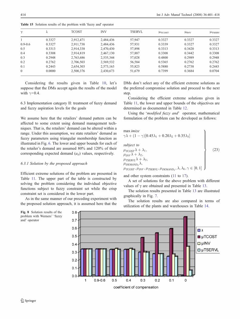
We assume here that the retailers’ demand pattern can beaffected to some extent using demand management tech-niques. That is, the retailers’ demand can be altered within arange. Under this assumption, we state retailers’ demand asfuzzy parameters using triangular membership function asillustrated in Fig. 6. The lower and upper bounds for each ofthe retailer’s demand are assumed 80% and 120% of theircorresponding expected demand (ail) values, respectively.

6.3.1 Solution by the proposed approach

Efficient extreme solutions of the problem are presented inTable 11. The upper part of the table is constructed bysolving the problem considering the individual objectivefunctions subject to fuzzy constraint set while the crispconstraint set is considered in the lower part.

As in the same manner of our preceding experiment withthe proposed solution approach, it is assumed here that the

DMs don’t select any of the efficient extreme solutions asthe preferred compromise solution and proceed to the nextstep.

Considering the efficient extreme solutions given inTable 11, the lower and upper bounds of the objectives aredetermined as documented in Table 12.

Using the ‘modified fuzzy and’ operator, mathematicalformulation of the problem can be developed as follows:

max imizeγλþ 1� γð Þ 0:45λ1 þ 0:20λ2 þ 0:35λ3½ �

subject toμTCOSTλþ λ1;μINVλþ λ2;μTSERVLλþ λ3;μDEMANDil

λ;μTCOST ;μINV ;μTSERVL;μDEMANDil

;λ;λk ; γ 2 0; 1½ �

9>>>>>>>>>>>=>>>>>>>>>>>;

ð23Þ

and other system constraints (11 to 17).A set of solutions for the above problem with different

values of γ are obtained and presented in Table 13.The solution results presented in Table 13 are illustrated

graphically in Fig. 7.The solution results are also compared in terms of

utilization of the plants and warehouses in Table 14.

Table 15 Solution results of the problem with 'fuzzy and' operator

γ λ TCOST INV TSERVL μTCOST μINV μTSERV

1 0.3327 2,912,471 2,484,436 57,947 0.3327 0.3327 0.33270.9-0.6 0.3327 2,911,738 2,484,436 57,931 0.3339 0.3327 0.33270.5 0.3313 2,914,338 2,470,430 57,898 0.3313 0.3420 0.33130.4 0.3308 2,914,819 2,467,130 57,887 0.3308 0.3442 0.33080.3 0.2948 2,763,686 2,535,344 57,028 0.4800 0.2989 0.29480.2 0.2762 2,706,503 2,569,532 56,584 0.5365 0.2762 0.27620.1 0.2443 2,654,303 2,573,163 55,823 0.5880 0.2738 0.24430 0.0000 2,500,376 2,430,673 51,679 0.7399 0.3684 0.0704

Fig. 8 Solution results of theproblem with Werners’ ‘fuzzyand’ operator


Comparing the results given in Table 13 together withconsideration of the utilization of the plants and ware-houses, let’s suppose that the DMs accept the results of themodel with γ=0.5, and that they consider this solution thepreferred compromise solution. Then, the procedure isterminated at Step 7.

If the results of the model with γ=0.5 are compared tothose of the model with γ=1, it can be realized thatsubstantial increase (45.9%) can be provided in achieve-ment level of the total cost objective with a decrease by11.7% in those of the second and third objective function.In terms of utilization rates of the plants and warehouses,the model with γ=0.5 provides better results compared tothe other solutions.

6.3.2 Solution by Werners’ ‘fuzzy and’ operator

Using Werners’ ‘fuzzy and’ operator, we obtain a set ofsolutions corresponding to different values of γ. The resultsare presented in Table 15 and illustrated graphically inFig. 8.

6.4 Comparison of the results

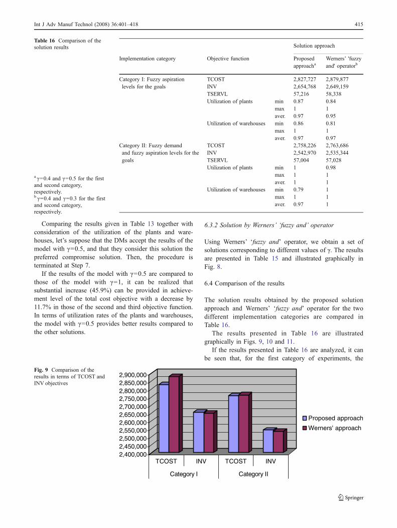
The solution results obtained by the proposed solutionapproach and Werners’ ‘fuzzy and’ operator for the twodifferent implementation categories are compared inTable 16.

The results presented in Table 16 are illustratedgraphically in Figs. 9, 10 and 11.

If the results presented in Table 16 are analyzed, it canbe seen that, for the first category of experiments, the

Table 16 Comparison of thesolution results

a γ=0.4 and γ=0.5 for the firstand second category,respectively.b γ=0.4 and γ=0.3 for the firstand second category,respectively.

Solution approach

Implementation category Objective function Proposedapproacha

Werners’ 'fuzzyand' operatorb

Category I: Fuzzy aspirationlevels for the goals

TCOST 2,827,727 2,879,877INV 2,654,768 2,649,159TSERVL 57,216 58,338Utilization of plants min 0.87 0.84

max 1 1aver. 0.97 0.95

Utilization of warehouses min 0.86 0.81max 1 1aver. 0.97 0.97

Category II: Fuzzy demandand fuzzy aspiration levels for thegoals

TCOST 2,758,226 2,763,686INV 2,542,970 2,535,344TSERVL 57,004 57,028Utilization of plants min 1 0.98

max 1 1aver. 1 1

Utilization of warehouses min 0.79 1max 1 1aver. 0.97 1

2,400,0002,450,0002,500,0002,550,0002,600,0002,650,0002,700,0002,750,0002,800,0002,850,0002,900,000

TCOST INV TCOST INV

Category I Category II

Proposed approach

Werners' approach

Fig. 9 Comparison of theresults in terms of TCOST andINV objectives


relative importance levels assigned to the membershipfunctions of the objectives can be reflected to the resultsto some extent by the proposed solution approach. Morespecifically, by using the proposed approach with givenweighting structure, total cost objective can be improved by1.81% while total service level objective is deteriorated by1.92%, and investment objective remains almost the samecompared to the results by Werners’ approach. On the otherhand, the results obtained by the proposed and Werners’approaches are almost the same for the second category ofexperiments. That is, the relative importance of theobjectives doesn’t influence on the results of the probleminstance. It can be concluded here that, the proposedsolution approach may provide different and even morepreferable results compared to the Werners’ ‘fuzzy and’approach. But, it should be emphasized that the weightstructure and the structure of the problem, e.g., fuzzy vs.crisp parameters, influences the level of differencesbetween the two approaches. The proposed IFGP-basedsolution approach can be employed by the DMs as aflexible and robust multi-objective decision making ap-proach to determine the preferred compromise solution.

7 Conclusions

A multi-objective linear programming model is developedin this paper to address the SC distribution network designproblem. The goal of the model is to select the optimumnumbers, locations and capacity levels of plants andwarehouses to deliver the products to the retailers at theleast cost while satisfying the desired service level. Themodel distinguishes itself from other models in this field inthe modeling approach used. Decision makers’ impreciseaspiration levels for the goals and retailers’ imprecisedemand are incorporated into the model using fuzzymodeling approach, which is otherwise not possible byconventional mathematical programming methods.

This paper also contributes to the literature by proposinga novel and generic IFGP-based solution approach whichdetermines the preferred compromise solution for multi-objective decision problems.

Results of the computational experiments performed onrealistic scale case problems explore the viability of theproposed solution approach and the SC distributionnetwork design model. The results also point out that SC

50,000

52,000

54,000

56,000

58,000

60,000

TS

ER

VL


Proposed approach

Werners' approach

Fig. 10 Comparison of theresults in terms of TSERVL

0.3

0.4

0.5

0.6

0.7

0.8

0.9

1

min aver. min aver. min aver. min aver.

Util.of plants Util. ofwarehouses

Util.of plants Util. ofwarehouses


Proposed approach

Werners' approach

Fig. 11 Comparison of theresults in terms of utilization ofthe plants and warehouses


distribution network design problem can be handled in amore flexible, robust and realistic way through theproposed model and the IFGP-based solution approach.

The proposed model can be used in real life industrialapplication in restructuring, i.e., expanding or narrowing, ofan existing SC distribution network besides the design of anew network. Such a strategic model can be a part of adecision support system developed for the collaborative SCmanagement practices.

References

1. Pirkul H, Jayaraman V (1998) A multi-commodity, multi-plant,capacitated facility location problem: formulation and efficientheuristic solution. Comput Oper Res 25(10):869–878

2. Jang Y-J, Jang S-Y, Chang B-Y, Park J (2002) A combined modelof network design and production/distribution planning for asupply network. Comput Ind Eng 43:263–281

3. Chopra S, Meindl P (2001) Supply chain management. PrenticeHall, Upper Saddle River, NJ

4. Church RL, Revelle C (1974) The maximal covering locationproblem. Pap Reg Sci Assoc 32:101–118

5. Zadeh LA (1965) Fuzzy sets. Inform Control 8:338–3536. Petrovic D, Roy R, Petrovic R (1999) Modeling and simulation of

a supply chain in an uncertain environment. Eur J Oper Res109:299–309

7. Reznik L, Pham B (2001) Fuzzy models in evaluation ofinformation uncertainty in engineering and technology applica-tions. Proceedings of the 10th IEEE International Conference onFuzzy Systems, Melbourne, Austraila, pp 972–975

8. Francis RL, Mcginnis LF, White JA (1983) Locational analysis.Eur J Oper Res 12:220–252

9. Aikens CH (1985) Facility location models for distributionplanning. Eur J Oper Res 22:263–279

10. Brandeau ML, Chiu SS (1989) An overview of representativeproblems in location research. Manage Sci 35:645–674

11. Beamon BM (1998) Supply chain design and analysis: modelsand methods. Int J Prod Econ 55:281–294

12. Avella P et al (1998) Some personal views on the current state andthe future of locational analysis. Eur J Oper Res 104:269–287

13. Pontrandolfo P, Okogbaa OG (1999) Global manufacturing: areview and a framework for planning in a global corporation. Int JProd Res 37(1):1–19

14. Meixell MJ, Gargeya VB (2005) Global supply chain design: aliterature review and critique. Transport Res E-Log 41:531–550

15. Geoffrion AM, Graves GW (1974) Multicommodity distributionsystem design by benders decomposition. Manage Sci 20(5):822–844

16. Brown GG, Graves GW, Honczarenko MD (1987) Design andoperation of a multicommodity production/distribution systemusing primal goal decomposition. Manage Sci 33(11):1469–1480

17. Cohen MA, Lee HL (1988) Strategic analysis of integratedproduction-distribution systems: models and methods. Oper Res36:216–228

18. Pirkul H, Jayaraman V (1996) Production, transportation, anddistribution planning in a multi-commodity tri-echelon system.Transport Sci 30:291–302

19. Jayaraman V (1998) An efficient heuristic procedure for practical-sized capacitated warehouse design and management. DecisionSci 29:729–745

20. Dogan K, Goetschalckx M (1999) A primal decompositionmethod for the integrated design of multi-period production anddistribution system. IIE Trans 31:1027–1036

21. Tragantalerngsak S, Holt J, Ronnqvist M (2000) An exact methodfor the two-echelon, single-source, capacitated facility locationproblem. Eur J Oper Res 123:473–489

22. Lee HK, Lee I-B, Reklaitis GV (2000) Capacity expansionproblem of multisite batch plants with production and distribution.Comput Chem Eng 24:1597–1602

23. Melachrinodis E, Min H (2000) The dynamic relocation andphase-out of a hybrid, two-echelon plant/warehousing facility: amultiple objective approach. Eur J Oper Res 123(1):1–15

24. Sabri EH, Beamon BM (2000) A multi-objective approach tosimultaneous strategic and operational planning in sc design.Omega 28:581–598

25. Pirkul H, Jayaraman V (2001) Planning and coordination ofproduction and distribution facilities for multiple commodities.Eur J Oper Res 133:394–408

26. Tsiakis P, Shah N, Pantelides CC (2001) Design of multi-echelonsupply chain networks under demand uncertainty. Ind Eng ChemRes 40:3585–3604

27. Talluri S, Baker RC (2002) A multi-phase mathematical program-ming approach for effective supply chain design. Eur J Oper Res141:544–558

28. Cakravastia A, Toha IS, Nakamura N (2002) A two-stage model forthe design of supply chain networks. Int J Prod Econ 80:231–248

29. Beamon BM, Fernandes C (2004) Supply chain network config-uration for product recovery. Prod Plan Control 15(3):270–281

30. Yeh W-C (2005) A hybrid heuristic algorithm for the multistagesupply chain network problem. Int J Adv Manuf Techol 26:675–685

31. Eskigun E, Uzsoy R, Preckel PV, Beaujon G, Krishnan S, Tew JD(2005) Outbound supply chain network design with modeselection, lead times and capacitated vehicle distribution centers.Eur J Oper Res 165:182–206

32. Amiri A (2006) Designing a distribution network in a supplychain: formulation and efficient solution procedure. Eur J OperRes 171:567–576

33. Narasimhan R (1980) Goal programming in a fuzzy environment.Decision Sci 11:325–336

34. Hannan EL (1981) Some further comments on fuzzy priorities.Decision Sci 13:337–339

35. Ignizio JP (1982) On the rediscovery of fuzzy goal programming.Decision Sci 13:331–336

36. Narasimhan R, Rubin PA (1984) Fuzzy goal programming withnested priorities. Fuzzy Set Syst 14:115–129

37. Tiwari RN, Dharmar S, Rao JR (1986) Priority structure in fuzzygoal programming. Fuzzy Set Syst 19:251–259

38. Tiwari RN, Dharmar S, Rao JR (1987) Fuzzy goal programming -an additive method. Fuzzy Set Syst 24:27–34

39. Bellman RE, Zadeh LA (1970) Decision making in a fuzzyenvironment. Manage Sci 17:141–164

40. Zimmermann H-J (1978) Fuzzy programming and linear program-ming with several objective functions. Fuzzy Sets Syst 1:45–55

41. Lai Y-J, Hwang C-L (1994) Fuzzy multiple objective decisionmaking. Springer, Berlin Heidelberg New York

42. Abd El-Wahed WF, Lee SM (2006) Interactive fuzzy goalprogramming for multi- objective transportation problems. Omega34:158–166

43. Werners B (1987) Interactive multiple objective programmingsubject to flexible constraints. Eur J Oper Res 31:342–349

44. Werners B (1987) An interactive fuzzy programming system.Fuzzy Set Syst 23:131–147

45. Leung Y (1987) Hierarchical programming with fuzzy objectivesand constraints. In: Kacprzyk J, Orlovski SA (eds) Optimizationmodels using fuzzy sets and possibility theory. D. Reidel,Dordrecht, pp 245–257


46. Fabian Cs, Ciobanu Gh, Stoica M (1987) Interactive polyopti-mization for fuzzy mathematical programming. In: Kacprzyk J,Orlovski SA (eds) Optimization models using fuzzy sets andpossibility theory. D. Reidel, Dordrecht, pp 272–291

47. Sasaki MY, Nakahara Y, Gen M, Ida K (1991) An efficientalgorithm for solving fuzzy multiobjective 0-1 linear program-ming problem. Comput Ind Eng 21:647–651

48. Babtistella LFB, Ollero A (1980) Fuzzy methodologies forinteractive multicriteria optimization. IEEE T Syst Man Cyb10:355–365

49. Werners B (1988) Aggregation models in mathematical program-ming. In: Mitra G, Greenberg HJ, Lootsma FA, Rijckaert MJ,Zimmermann H-J (eds) Mathematical models for decisionsupport. Springer, Berlin Heidelberg New York, pp 295–305


a supply chain distribution network design model: an ...ceit.aut.ac.ir/~sa_hashemi/my...

Documents