A subexponential parameterized algorithm for Subset TSP on planar

graphs

Philip N. Klein∗ Daniel Marx†

Abstract

Given a graph G and a subset S of vertices, the SubsetTSP problem asks for a shortest closed walk in Gvisiting all vertices of S. The problem can be solved intime 2k ·nO(1) using the classical dynamic programmingalgorithms of Bellman and of Held and Karp, where k =|S| and n = |V (G)|. Our main result is showing that the

problem can be solved in time (2O(√k log k) +W ) · nO(1)

if G is a planar graph with weights that are integersno greater than W . While similar speedups have beenobserved for various paramterized problems on planargraphs, our result cannot be simply obtained as aconsequence of bounding the treewidth of G or invokingbidimensionality theory. Our algorithm consists of twosteps: (1) find a locally optimal solution, and (2) use itto guide a dynamic program. The proof of correctnessof the algorithm depends on a treewidth bound on agraph obtained by combining an optimal solution witha locally optimal solution.

1 Introduction

The Traveling Salesperson Problem (TSP) is one of themost famous and most studied combinatorial optimiza-tion problems. Given a pair (S, d(·, ·)) where S is afinite set and d : S × S −→ R is a weight function, atour is a permutation cycle (s0 . . . sk−1). The weight ofa tour is

∑i d(si, si+1 (mod k)), and the goal is to find

a minimum-weight tour. We use k for the size of S.An easy reduction from Hamiltonian Cycle showsthat the problem is NP-hard even if every weight is 1or 2. The problem can be solved by enumerating all the(k − 1)! tours, or more efficiently, by the classical dy-namic programming algorithms of Bellman [4] and Heldand Karp [17] solving 2k subproblems.

∗Brown University, Providence, Rhode Island, USA. Researchsupported by National Science Foundation Grant CCF-0964037.†Institute of Computer Science and Control, Hungarian

Academy of Sciences (MTA SZTAKI), Budapest, Hungary. Re-search supported by the European Research Council (ERC) grant“PARAMTIGHT: Parameterized complexity and the search for

tight complexity results,” reference 280152 and OTKA grantNK105645.

Metric TSP is the special case when the pair(S, d) is a metric space, that is, the distances aresymmetric and satisfy the triangle inequality. Thisproblem is equivalent to finding a minimum-weight walkin an undirected graph with nonnegative symmetricedge-weights, for one can define S to be the vertex setand d(u, v) to be the u-to-v distance (this is the metriccorresponding to the edge-weighted graph). MetricTSP has a polynomial-time 3

2 -approximation due toChristofides [7]. Various special cases of Metric TSPor the related Hamiltonian Cycle problem are knownto be solvable in time cn for different constants c < 2[14, 5, 18, 13]. However, in general graphs, we do notexpect algorithms with running time 2o(n) for MetricTSP, as this would contradict the Exponential TimeHypothesis (ETH), see, e.g., the survey [27].

The problem becomes significantly easier when themetric is the Euclidean metric between points in theplane. For this problem, polynomial-time approxima-tion schemes are known [1, 29, 30]. Moreover, there isa 2O(

√n log n)-time algorithm to find the optimum solu-

tion [32].The problem also becomes significantly easier when

the metric is given by distances in a planar graph. First,it admits a polynomial-time approximation scheme(PTAS) ([15] for the case of unit weights) and ([2]for general weights) and even a linear-time approxi-mation scheme [22, 24]. For finding an exact solution,the well-known fact that an n-vertex planar graph hastreewidth O(

√n) [31] combined with standard tech-

niques for solving TSP on bounded-treewidth graphsyield a 2O(

√n log n)-time algorithm [8]. Using noncross-

ing properties with a Catalan bound yields a 2O(√n)-

time algorithm [12].One motivation for studying Metric TSP where

the metric is given by distances in a planar graph isthat a road network can be modeled by a planar graph(ignoring overpasses etc.). However, this formulationrequires the tour to visit every road intersection, whichis not very realistic. This suggests the Subset TSPproblem: given a graph G and a subset S ⊆ V (G)of vertices, the task is to find the shortest closed walkvisiting every vertex of S (and possibly other vertices).

We refer to the vertices in S as terminals.For general graphs, Subset TSP can be modeled

by just starting with the metric space correspondingto G and then taking the submetric induced on S.However, even when G is planar, the submetric isnot in general the metric corresponding to a planargraph, so Subset TSP restricted to planar graphsis a strict generalization of Metric TSP restrictedto planar graphs. Indeed, this problem is also astrict generalization of Metric TSP restricted to theEuclidean metric of points in the plane: a planarembedded graph can be constructed by taking the linesegments between the given points, and introducing newvertices at the crossings.

Do the favorable algorithmic properties of MetricTSP on planar graphs carry over to Subset TSP prob-lem? It has been shown that this generalization has anO(n log n) approximation scheme [23]. Moreover, usingstandard techniques for bounded-treewidth graphs, theproblem can be solved exactly in time 2O(

√n log n). But

note that the number k of terminals is likely to be muchsmaller than the total number of vertices. By disregard-ing planarity, one can use the classical DP approach onthe submetric to solve the problem exactly in 2k · nO(1)

time. Can we do better by exploiting planarity? Inparticular, can we get an exact algorithm whose run-ning time is polynomial in n and whose dependence onk improves over that of the general algorithm? Ourmain result is a positive answer to this question:

Theorem 1.1. Subset TSP on a planar n-vertexgraph with k terminals can be solved in time

(2O(√k log k) + W ) · nO(1) if the weights are integers no

greater than W .

As we have observed above, Theorem 1.1 cannotbe obtained by simply observing that the n-vertexplanar graph G has treewidth O(

√n), as this leads

only to 2O(√n log n) time algorithms. Bidimensionality

theory [10, 9] gives parameterized algorithms on planar

graphs with running time of the form 2O(√k) · nO(1)

or 2O(√k log k) · nO(1) for a number of problems such as

finding an independent set of size k or finding a cycleof length at most k. The main idea of these algorithmsis that either the graph contains an Ω(

√k) × Ω(

√k)

grid minor, in which case we can immediately get ananswer, or the graph has no such grid, in which casewe can conclude that the graph has treewidth O(

√k)

and hence standard techniques on bounded-treewidthgraphs can be used. This approach does not seem towork for Subset TSP: it is not clear what we canconclude from the existence of an Ω(

√k)× Ω(

√k) grid

minor in this problem.Our algorithm eventually relies on the fact that an

O(k)-vertex planar graph G has treewidth O(√k), but

we have to adopt a different viewpoint in order to beable to exploit this combinatorial relation. First, let usreview how TSP can be solved in time 2k · nO(1) usingdynamic programming [4, 17]. Let us fix an arbitrarystart vertex v0. For every vertex x and subset S′ ⊆ S,we define the subproblem (x, S′), which is the minimumlength of a path from v0 to x that visits exactly theterminals in S′. It can be shown that if we have solvedall the subproblems with |S′| = i, then the subproblemswith |S′| = i+1 can be solved using a simple recurrencerelation. The subproblem (x, S) tells us the minimumlength of a path from v0 to x visiting all vertices andit is easy to deduce the minimum length of the tourfrom these subproblems. The dominating factor of therunning time comes from the number of subproblems,which is k · 2k.

We can try to generalize the algorithm described inthe previous paragraph the following way. Instead ofrequiring a path from v0 to x visiting a certain set S′,we require a family of at most p paths with specifiedendpoints such that these paths together visit everyvertex of S′. The family of paths can be specified by 2pendpoints, which adds a factor of kO(p) to the numberof subproblems; as long as p = O(

√k), this is only

2O(√k log k). One could expect that by keeping track

of O(√k) paths, the algorithm becomes more powerful

and perhaps finds the optimum solution more efficiently.While this might be true, the main bottleneck of thealgorithm is the number of possible such sets S′, whichis still 2k. Thus if we want to improve the running timebeyond 2k, we need to find a way of considering onlya restricted collection S of subsets S′, instead of all 2k

possible subsets of S.One of the main technical ideas of the paper appears

in the way this restricted collection S of subsets isconstructed. The construction is based on a locallyoptimal solution. First, by the symmetry of the weightfunction, the weight of a tour is the same as the weightof its reversal. Up to reversal, a tour is specified byan undirected graph on vertex set S whose edges forma simple cycle. Therefore, we henceforth use the termS-tour (or just tour if the choice of S is clear) to referto such a graph.

A popular heuristic for symmetric TSP is based oniteratively improving a tour by making small changes.For a number c, a c-change in a tour consists of removingc edges to split the tour into c paths and then addingc new edges to reconnect the endpoints of these pathsand obtain a new tour. We say that a tour is a c-opttour with respect to the metric d(·, ·) if no such movecan strictly improve the length of the tour. Finding2-opt or 3-opt tours form the basis of many heuristic

algorithms [26, 19, 20, 21].The following bound is the main combinatorial re-

sult of the paper: it bounds the treewidth of combiningan optimal tour and a 4-opt tour. For technical reasons,we need to impose an additional condition on the 4-opttour. We say a tour is non-self-crossing with respectto the planar embedded graph G if it corresponds to anon-self-crossing walk in G (see Section 2 for details).

Theorem 1.2. Let G be a planar embedded graph, letS be a set of k terminals, and let (S, d(·, ·)) be thecorresponding metric space. Let T4 be an S-tour thatis 4-opt with respect to d(·, ·) and non-self-crossing withrespect to G. Then there is an optimal tour Topt withrespect to d(·, ·) such that the k-vertex graph formed bythe union of the cycles T4 and Topt has treewidth at most

α√k, where α is a universal constant.

Note that this is a purely combinatorial statement andgives no algorithm for finding the optimum or comput-ing a tree decomposition of the union. Nevertheless, weconclude from Theorem 1.2 that it is sufficient to formthe restricted collection S of subsets of S by taking ev-ery possible union of O(

√k) consecutive segments of T4.

For this choice, the size of S is kO(√k) = 2O(

√k log k). A

subproblem is defined by specifying O(√k) endpoints

for the paths and selecting a member of S, hence the

number of subproblems is also 2O(√k log k).

In summary, the algorithm works as follows. First,we find a non-self-crossing 4-opt S-tour in polynomialtime by iterative improvement. Then we construct acollection of subsets by taking every possible union of

O(√k) consecutive segments of T4 and define 2O(

√k log k)

types of partial solutions; each type is defined byfixing the endpoints of O(

√k) paths and selecting a

subset from our collection. Starting with some trivialpartial solutions, we present a way of combining partialsolutions to obtain larger partial solutions. We usethe tree decomposition given by Theorem 1.2 to provethat this process of combining partial solutions willeventually lead to an optimum solution for the wholeproblem.

Strictly speaking, our algorithm cannot be calleddynamic programming. The usual meaning of dynamicprogramming is that we specify some number of well-defined subproblems and then we provide a correctanswer for each of these subproblems in some order,based on the answers for earlier subproblems. In ouralgorithm, we define types of partial solutions, but wedo not claim in any way that we find an optimal partialsolution for each type. What we show is that theoperation of combining partial solutions gives optimalpartial solutions for certain types, including the typethat represents the whole problem. More precisely, the

types that are guaranteed to be solved optimally dependon the tree decomposition given by Theorem 1.2. Asthis is a purely existential statement, we do not knowduring the execution of the algorithm which are thetypes that are guaranteed to be solved optimally, withthe exception of the one representing the whole, whichis always solved optimally.

Let us emphasize that, even though treewidth ap-pears in a crucial way in the analysis of our algorithm, itis never explicitly used by the algorithm. In particular,we do not find tree decompositions or solve any problemusing dynamic programming on a given tree decomposi-tion. The tree decomposition is used only in the analy-sis of the algorithm to argue that we get optimal partialsolutions for certain types. This way of using a tree de-composition without actually having the decompositionat hand is very similar to how consistency-based algo-rithms solve CSP instances of bounded width, see, e.g.,[3, 6].

We would like to dispel a possible source of confu-sion. Based on Theorem 1.2 and the way we constructthe collection S using O(

√k) segments of T4, the reader

might have the impression that the optimum solutioncan be obtained from T4 by O(

√k) changes. If this

were true, then any O(√k)-change optimal tour would

be globally optimal, and then we could obtain an opti-mum solution in a much simpler way, without the com-plicated process of combining partial solutions. How-ever, we show an example where even an Ω(k)-changeoptimal tour is not globally optimal. Intuitively, eventhough the locally optimal tour can be considered “sim-ilar” to an optimal tour, the similarity can be more sub-tle than what can be expressed by a simple change ofordering.

As noted earlier, Subset TSP in the metric arisingfrom a planar graph is a generalization of the problemof finding a minimum-length tour of points in the plane.Our algorithm can therefore be applied to this problem.Note that a 4-opt solution for such a Euclidean instanceis automatically non-self-crossing. For such an instance,we do not have a good bound on the number of iterationsof local search required to achieve a 4-opt solution andtherefore on the running time (although reportedly localsearch tends to terminate quickly in practice). However,the running time of our algorithm if given a 4-opt

solution matches the 2O(√k log k) running time of [32]

up to the constant hidden by the big-O.The paper is organized as follows. Section 2 intro-

duces notation and contains some preliminary results onnon-self-crossing tours, local search, and tree decompo-sitions. The main algorithm is described in Section 3.The proof of Theorem 1.2 appears in Section 4.

t t' t

(a) Replacing a terminal t with a degree-1 terminal t′.

(b) This figure shows that we may assume that a realizationuses each edge at most once in each direction. By requiringthat each edge is one of several parallel edges, we can thereforeassume that a realization uses each edge at most once.

Figure 1: Two transformations

2 Preliminaries

We present some of the background and technical toolsnecessary for our algorithm in this section. We formallydiscuss the fact that tours can be represented in twodifferent ways (ordering of the terminals or a closed walkin the graph), define local optimality, and introducetreewidth.

2.1 Tours and realizations An S-tour is a graphwith vertex set S whose edges form a simple cyclevisiting all vertices. Let G be a graph whose vertex setincludes S. We refer to the vertices of S as terminals.A realization of an S-tour in G is a walk that visits theterminals in the same cyclic order as the S-tour.

It is convenient to impose the requirement on Gthat each terminal is adjacent in G to exactly oneother vertex. If some terminal t has more than oneneighbor, replace it with an artificial node t′ andattach t to t′ via a zero-weight edge (see Figure 1a).Under this requirement, we can restrict our attentionto realizations in which each terminal occurs exactlyonce.

It is also convenient to require that each edge of Gis one of four parallel edges. Under this requirement,we can restrict our attention to realizations in whicheach edge occurs at most once. (The argument usesthe modification shown in Figure 1b.) In fact, whenconsidering a pair of tours, we can assume in additionthat the tours are edge-disjoint.

Now let us also assume G is planar embedded. Leta1va2 and b1vb2 be two-edge paths sharing the samemiddle vertex v. We say these two paths form a crossing

v

(a) A crossing.

(b) Uncrossing a self-crossing walk.

Figure 2: Crossing and uncrossing

at v if in the cyclic order of edges about v, the edgesalternate between edges from a1v, a2v and edges fromb1v, b2v (see Figure 2a). We say a walk is self-crossingif it contains subpaths that form a crossing. Given aclosed walk that is self-crossing, one can obtain a closedwalk that is non-self-crossing and uses the same edgesby repeating the step illustrated in Figure 2b. Note thatwhen this step is applied to the realization of an S-tour,the result might be a realization of a different S-tour.We say an S-tour is non-self-crossing with respect to agraph G if the S-tour has a non-self-crossing realizationin G.

Now let G have nonnegative edge-weights. For a setA of edges with weights, w(A) denotes the total weight.Define the metric d(·, ·) by letting d(s, s′) to be the s-to-s′ distance in G. Given the graph G and any S-tourT , we can find a realization W of minimum weight byfinding shortest paths between vertices of S consecutivein the S-tour. Then we can uncross this this realizationto obtain a non-self-crossing closed walk W ′. However,after uncrossing, the walk W ′ might visit the verticesof S in a different order than T . Nevertheless, basedon W ′ we can define an S-tour T ′ such that W ′ is arealization of T .

Proposition 2.1. Given a graph G and an S-tour T ,we can find in polynomial time a non-self-crossing S-tour T ′ with cost not more than the cost of T .

2.2 Locally optimal tours Given two S-tours T1

and T2, the distance between T1 and T2 is defined as|E(T1) \ E(T2)| = |E(T2) \ E(T1)|. We say that anS-tour T is c-opt if there is no tour T ′ at distance atmost c with w(T ′) < w(T ). For a fixed constant c,one can use brute force to check in polynomial timeif a tour is c-opt, and if not, find a tour with strictly

smaller weight. By repeatedly searching the distance-c neighborhood and replacing the current solution if abetter solution is found, eventually one arrives to a c-optsolution. The sequence of improvements until we reacha c-opt solution can be very long, but if the weights arepositive integers, then we can bound the length of thesequence by the maximum weight of a tour.

Proposition 2.2. Let G be a weighted graph where ev-ery weight is a positive integer not larger than W . Thena c-opt S-tour can be found in time (|S|c)c|V (G)|O(1)W .

Note that finding a better solution in the c-changeneighborhood is W[1]-hard [28] parameterized by c, thusit seems that c has to appear in the exponent of therunning time.

In our algorithm, we need to work with non-self-crossing S-tours. After each step of the iterativeimprovement, we can find a non-self-crossing S-tourof the same cost using Proposition 2.1. Therefore, byinterleaving the local improvement and the uncrossingstep, we get the following algorithm:

Proposition 2.3. Let G be a weighted planar embed-ded graph where every weight is a positive integer notlarger than W . Then a non-self-crossing c-opt S-tourcan be found in time (|S|c)4|V (G)|O(1)W .

2.3 Treewidth We recall the most important no-tions related to treewidth in this section.

Definition 2.1. A tree decomposition of a graph G isa pair (T,B) in which T is a tree and B = Bt|t ∈ V (T )is a family of subsets of V (G) such that

1.⋃

t∈V (T )Bi = V ;

2. for each edge e = uv ∈ E(G), there exists ant ∈ V (T ) such that both u and v belong to Bt; and

3. the set of nodes t ∈ V (T ) | v ∈ Bt forms aconnected subtree of T for every v ∈ V (G).

To distinguish between vertices of the original graph Gand vertices of T in the tree decomposition, we callvertices of T nodes and their corresponding Bi’s bags.The width of the tree decomposition is the maximumsize of a bag in B minus 1. The treewidth of a graphG, denoted by tw(G), is the minimum width over allpossible tree decompositions of G.

A tree decomposition is nice [25] if it has thefollowing property: every node t ∈ V (T ) is either

• a leaf node (t has no children and |Bt| = 1),• a join node (t has two children t′, t′′ and Bt′ = Bt′′),

• a forget node (t has a single child t′ and Bt ⊆ Bt′ ,|Bt| = |Bt′ | − 1), or

• an introduce node (t has a single child t′ and Bt ⊇Bt′ , |Bt| = |Bt′ |+ 1).

It is known that every tree decomposition can be turnedinto a nice tree decomposition of the same width inpolynomial time. We often assume that the tree isrooted.

We need the following bound on the treewidth ofplanar graphs:

Theorem 2.1. ([31]) The treewidth of a planar graphon k vertices is O(

√k).

Tutte proved that any 2-connected graph has a de-composition into 3-connected components. This resultcan be stated in modern terms using tree decomposi-tions the following way. First, we need the definition oftorso. Let (T,B) be a tree decomposition. The torsoat t is defined as the supergraph of G[Bt] obtained byadding a clique on Bt ∩Bt′ for every neighbor t′ of t inT . The following theorem states that every graph canbe decomposed into 3-connected components. We willuse this statement in the proof of Theorem 1.2, whenwe focus on 3-connected parts of a certain graph.

Theorem 2.2. (cf. [11, Section 12, Ex. 20] [16])Every 2-connected graph has a tree decomposition(T,B), where

• |Bt ∩Bt′ | = 2 for every tt′ ∈ E(T ),

• for every t ∈ V (T ), the torso at t is either 3-connected or is a complete graph of size at most3.

A 2-separator is a set Z = x, y of vertices whoseremoval splits the graph into at least two components.Note that if (T,B) is the tree decomposition of a 2-connected graph given by Theorem 2.2, then Bt′ ∩ Bt′′

is a 2-separator for every t′t′′ ∈ E(T ), and conversely,every 2-separator can be obtained this way.

The following statement appears implictly in earlierwork: it allows us to bound treewidth by bounding thetreewidth of 3-connected components. We provide ashort proof for completeness.

Proposition 2.4. Let (T,B) be a tree decompositionof a graph G such that the torso at every t ∈ V (T ) hastreewidth at most w. Then G has treewidth at most w.

Proof. Let t be a node of T such that |Bt| > w + 1.Let G∗t be the torso at t. By assumption, G∗t has a treedecomposition (T ∗t ,B∗t ) of width at most w, which isalso a tree decomposition of G[Bt]. We modify (T,B)to obtain another decomposition (T ′,B′) of G. We

construct T ′ by removing node t, adding the tree T ∗t ,and then connecting T ∗t to T \ t the following way. Fora neighbor t′ of t in T , let Zt = Bt ∩ Bt′ ; note that Zt

induces a clique in G∗t . It is well-know that every cliqueis covered by some bag of the tree decomposition; lett∗ ∈ V (T ∗t ) be such that Zt ⊆ Bt. Then we maket′ adjacent to t∗. Repeating this process for everyneighbor t′ of t, we indeed get a tree decomposition(T ′,B′) of G. For every t∗ ∈ T ∗t , the size of Bt∗ is atmost w + 1, thus (T ′,B) has one fewer bags with sizegreater than w + 1. Therefore, repeating this processfor every such bag gives the desired tree decomposition.

3 Algorithm

We describe our main algorithm in Section 3.1. Thealgorithm takes a set of “admissible types” as an input.In Section 3.2, we define a particular set of admissibletypes and we prove (using Theorem 1.2) that thealgorithm finds an optimum solution if this set is givenin the input.

3.1 Building partial solutions Let (S, d(·, ·)) be asubmetric space of the metric space defined by distancesin a planar graph with edge-weights. Let G be thecomplete edge-weighted graph with vertex set S wherethe weight of ss′ is d(s, s′). We assume |S| ≥ 3.

A partial solution H is a subgraph of G that is eitherthe vertex-disjoint union of paths or a cycle containingall k = |S| vertices. We denote by s(H) the nonisolatedvertices of H, which we refer to as the set of verticesvisited by the partial solution. We denote by ε(H) theendpoints of the paths (of length at least 1) in H; ifH is a cycle visiting all vertices, then ε(H) = ∅. Theweight w(H) of a partial solution H is the total weightof the edges in H. Given a partial solution H, wedefine a matching m(H) on the set ε(H) as follows:x, y ∈ ε(H) are matched in m(H) if H contains a pathwith endpoints x and y. Clearly, m(H) is a perfectmatching of ε(H). The type of the solution is the pair(s(H),m(H)).

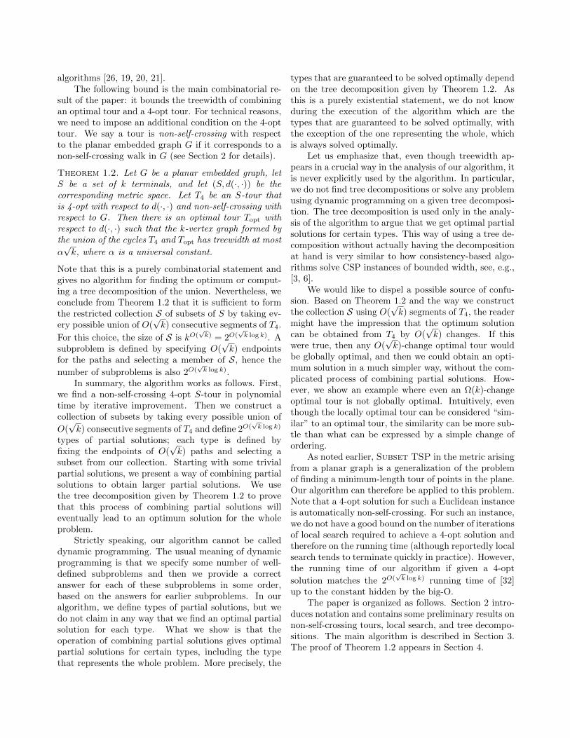
Note that the type does not describe which pathvisits which vertices, it describes only the total set ofvertices visited and the endpoints of the paths (seeFigure 3). The number of edges of the subproblem canbe deduced from the type: it is exactly s(H) minusthe number of edges in m(H). Observe that for everypartial solution with at most two edges, there is no otherpartial solution with the same type. However, this isnot true for partial solutions with 3 edges: the partialsolution consisting of the path v1v2v3v4 and the partialsolution consisting of the path v1v3v2v4 have the sametype (v1, v2, v3, v4, v1v4).

1 2

56

7

8 3

4

1 2

56

7

8 3

4

Figure 3: Two partial solutions of type(1, 2, 3, 4, 5, 6, 8, 12, 45).

1 2

56

7

8 3

4

1 2

56

7

8 3

4

1 2

56

7

8 3

4

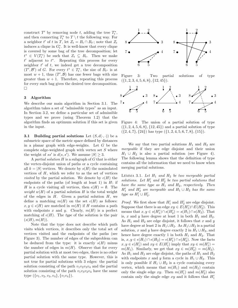
Figure 4: The union of a partial solution of type(1, 2, 4, 5, 6, 8, 12, 45) and a partial solution of type(2, 4, 7, 24) has type (1, 2, 4, 5, 6, 7, 8, 15).

We say that two partial solutions H1 and H2 aremergeable if they are edge disjoint and their unionH1 ∪ H2 is also a partial solution (see Figure 4).The following lemma shows that the definition of typecontains all the information that we need to know whenmerging partial solutions.

Lemma 3.1. Let H1 and H2 be two mergeable partialsolutions. Let H ′1 and H ′2 be two partial solutions thathave the same type as H1 and H2, respectively. ThenH ′1 and H ′2 are mergeable and H1 ∪ H2 has the sametype as H ′1 ∪H ′2.

Proof. We first show that H ′1 and H ′2 are edge disjoint.Suppose that there is an edge xy ∈ E(H ′1)∩E(H ′2). Thismeans that x, y ∈ s(H ′1)∩s(H ′2) = s(H1)∩s(H2). Thatis, x and y have degree at least 1 in both H1 and H2.As H1 and H2 are edge disjoint, it follows that x and yhave degree at least 2 in H1∪H2. As H1∪H2 is a partialsolution, x and y have degree exactly 2 in H1 ∪H2, andhence have degree exactly 1 in both H1 and H2. Thatis, x, y ∈ ε(H1) ∩ ε(H2) = ε(H ′1) ∩ ε(H ′2). Now the factsx, y ∈ ε(H ′1) and xy ∈ E(H ′1) imply that xy ∈ m(H ′1) =m(H1). Similarly, we get that xy ∈ m(H ′2) = m(H2).As H1 and H2 are edge disjoint, the paths of H1 and H2

with endpoints x and y form a cycle in H1 ∪H2. Thisis only possible if H1 ∪ H2 is a cycle containing everyvertex, which means that m(H1) and m(H2) containonly the single edge xy. Then m(H ′1) and m(H ′2) alsocontain only the single edge xy and it follows that H ′1

and H ′2 contain only the single edge xy. Therefore,s(H ′1) = s(H ′2) = s(H1) = s(H2) = x, y and hences(H1 ∪H2) = x, y, contradicting that H1 ∪H2 visitsevery vertex and the assumption |S| ≥ 3.

Clearly, s(H1 ∪ H2) = s(H1) ∪ s(H2) = s(H ′1) ∪s(H ′2) = s(H ′1 ∪ H ′2). It is easy to see that thecomponents of H1∪H2 are described by the componentsof the graph m(H1)∪m(H2) in the sense that for everypath of H1∪H2, there is a path of m(H1)∪m(H2) withthe same endpoints and vice versa. (If H1∪H2 is a cyclevisiting every vertex, then m(H1) ∪ m(H2) is a singlecycle). In other words, m(H1 ∪ H2) is the matchingdefined by the endpoints of the paths in m(H1)∪m(H2).As m(H ′1) ∪m(H ′2) = m(H1) ∪m(H2), we can deducethat the components of H ′1∪H ′2 are paths with the samepair of endpoints as in H1 ∪H2. Therefore, H ′1 ∪H ′2 isalso a partial solution and m(H ′1 ∪H ′2) = m(H1 ∪H2).

Our algorithm starts with an initial set P of partialsolutions (e.g., those containing only a single edge) andthen creates new partial solutions by taking the union ofmergeable pairs. For each type, we keep only one partialsolution: the one with the smallest weight found so far.By considering the mergeable pairs in increasing orderof the number of edges (see later for details), one canshow that the running time is polynomial in the numberof types. However, the number of types is bounded frombelow by the number of subsets of S, which is 2k, andthe number of matchings, which is 2Ω(k log k), thus there

is no hope of obtaining a 2O(√k log k) time algorithm if

we consider every possible type.In order to decrease the running time, we restrict

our attention to a subset of all possible types. Let Tbe a set of types, which we call the admissible types.Our algorithm merges two partial solutions only if thetype of the resulting new partial solution is admissible.Since the running time can be bounded by the numberof admissible types, it suffices to show that we canconstruct a set T of admissible types that is sufficiently

small to keep the running time 2O(√k log k), but at

the same time sufficiently large to guarantee that anoptimum solution is found. Section 3.2 presents a wayof construction such a collection.

The algorithm BuildSolutions is presented for-mally in Algorithm 1. Given a set T of admissible typesand a set P of admissible partial solutions, the algo-rithm repeatedly merges partial solutions to obtain newpartial solutions having admissible types. From each ad-missible type, the algorithm keeps only the best solutionof that type found so far. The algorithm performs themerges in a specific order to avoid the situation wheretwo partial solutions H1 and H2 are merged, but later

a there emerges another partial solution H ′1 of the sametype as H1 and having smaller weight. For increasingvalues of i, the algorithm considers merges where H1

and H2 have less than i edges, but H1 ∪H2 has at leasti edges. This ensures that after the first time a partialsolution H is used in a merge, no new partial solutionwith the same type as H is created. The result H1∪H2

of the merge is introduced into P if either P has nopartial solution of this type, or the partial solution ofthis type in P has strictly larger weight. At the endof the algorithm, if P contains a solution of type (S, ∅)(that is, a cycle visiting every vertex), then the algo-rithm returns it. Note that, depending on the set T ,the algorithm might not be able to create such a solu-tion and even if it creates one, there is no guaranteethat it is a minimum weight cycle visiting every vertex.The size of P is always at most |T |. For each value of i,the algorithm performs at most |P|2 merge operations.We therefore obtain the following.

Proposition 3.1. The number of steps ofBuildSolutions is polynomial in |T | and k.

3.2 Admissible types We construct a set T ofadmissible types in the following way. First, we computea non-self-crossing 4-opt tour T4 using the algorithmof Proposition 2.1. A continuous sequence of verticesvisited by T4 will be called a segment of T4. LetD := max4, dα

√ke + 1 = O(

√k), where α is the

constant in Theorem 1.2. The type τ = (S′,M) appearsin T if and only if

• S′ can be formed as the union of at most Dsegments of T4, and

• M has at most D edges.

The hidden constant in the big-O notation comes from

Theorem 1.2. It is clear that |T | = kO(√k) = 2O(

√k log k)

and T can be constructed in time polynomial in Tand k. We initialize P by introducing every partialsolution with only one edge (there are

(k2

)of them).

For notational convenience, we also add the emptypartial solution of type (∅, ∅) into P. We run thealgorithm BuildSolutions on the sets T and P.The correctness of the algorithm crucially relies onTheorem 1.2, stated in the introduction. We are nowready to show that OptimalTSP (Algorithm 2) findsan optimum solution, proving Theorem 1.1. The proofshows that partial solutions corresponding to the treedecomposition given by Theorem 1.2 have to eventuallyappear in P.

Algorithm 1 BuildSolutions(T ,P)

Input:T : set of admissible typesP: initial set of admissible partial solutions

1: for i = 2 to k2: for every pair H1, H2 ∈ P with |E(H1)|, |E(H2)| < i3: if H1 and H2 are mergeable and |E(H1 ∪H2)| ≥ i4: let τ = (S′,M) be the type of H1 ∪H2

5: if τ ∈ T and P contains no partial solution of type τ6: P := P ∪ H1 ∪H27: if there is a H ∈ P having type τ and w(H) > w(H1 ∪H2)8: P := (P \ H) ∪ H1 ∪H29: return the partial solution in P having type (S, ∅) (if exists)

Algorithm 2 OptimalTSP(G,S)

Input:G: a planar graph.S: k-element subset of V (G).

1: Compute the metric d(·, ·) on S.2: Find a non-self-crossing 4-opt tour T4.3: Let D := max4, dα

√ke+ 1. α is the constant in Theorem 1.2

4: Let T contain every type τ = (S′,M) where– S′ is the union of at most D segments of T4, and– M is a matching of at most D edges.

5: Let P contain– the empty partial solution, and– the

(k2

)partial solutions with one edge each.

6: return BuildSolutions(T ,P).

For the reader’s convenience, we restate the theo-rem:

Subset TSP on a planar n-vertex graph with

k terminals can be solved in time (2O(√k log k)+

W ) ·nO(1) if the weights are integers no greaterthan W .

Proof. of Theorem 1.1. We show that the algorithmOptimalTSP solves the problem. The bound on therunning time is straightforward: the non-self-crossing4-opt solution T4 can be found in time kO(1) ·W using

Proposition 2.3, the set T has size 2O(√k log k), and the

number of steps of BuildSolutions is polynomial in Tand k. To argue that the algorithm finds an optimumsolution, let Topt be the optimum solution and let αbe the constant in Theorem 1.2. Let (T,Bt) be arooted nice tree decomposition of T4 ∪ Topt (the graphrepresenting the combination of the two tours) havingwidth at most α

√k. For every node t, let Vt be the

union of Bt′ for every descendant t′ of t (including titself). We define Pt = Topt[Vt] and P−t as Pt minus theedges induced by Bt. Observe that P−t is also a partial

solution.

Claim 3.2. For every t ∈ V (T ), the partial solutionsPt and P−t are admissible.

Proof. Let St and S−t be the set of nonisolated verticesof Pt and P−t , respectively. Note that these sets aresubsets of Vt, but can be proper subsets as, e.g., a vertexv ∈ Bt can have both of its neighbors in Topt outsideVt, making v isolated in Pt. The set St induces a setof d disjoint paths on T4. We claim that each of the 2dendpoints of these paths is either in Bt or is a neighborof Bt in T4. Indeed, if a vertex v is in Vt\N [Bt], then itsneighbors are in Vt\Bt, and all these vertices are visitedby Pt, thus v cannot be an endpoint. Therefore, wecan bound the number 2d of endpoints by |Bt| plus thenumber of neighbors of Bt in T4. More tightly, observethat if v ∈ Bt is an endpoint of a path in G[St] and v1, v2

are the neighbors of v in T4, then v1 and v2 cannot beboth endpoints. Thus we can be bound the number 2dof endpoints by 2|Bt|, that is, St induces a set of at mostd ≤ |Bt| ≤ α

√k + 1 ≤ D paths in T4. This means that

Pt is admissible. The same argument shows that P−t is

admissible as well. y

By the way we initialized P, every partial solution withat most one edge is in P. Moreover, in iteration i = 2of BuildSolutions, we merge these partial solutionsevery possible way and therefore every partial solutionwith at most two edges is in P. (This is no longertrue for partial solutions consisting of 3 edges: thepartial solution consisting of the path v1v2v3v4 andthe partial solution consisting of the path v1v3v2v4

have the same type, hence they cannot both appearin P). Furthermore, as D ≥ 4 (defined in Step 3 ofAlgorithm 2), every partial solution with at most 2edges is admissible.

Claim 3.3. For every t ∈ V (T ),

• after iteration i = |E(Pt)|, there is a Qt ∈ P withthe same type as Pt and w(Qt) ≤ w(Pt),

• after iteration i = |E(P−t )|, there is a Q−t ∈ P withthe same type as P−t and w(Q−t ) ≤ w(P−t ).

Proof. Note that if a partial solution with i edgesappears in P at the end of iteration i, then it remainsin P until the end of BuildSolutions: in iterationslarger then i, only types corresponding to more thani edges are updated. We prove the statement byinduction on the tree decomposition. Let us assumethat the statement is true for every child t′ of t. Weconsider the different cases corresponding to the type ofthe node t.

• Node t is a leaf node. In this case Vt = Bt has size1, thus Pt and P−t has no edges. As P contains theempty solution, the statement holds.

• Node t is an introduce node with child t′. LetBt \ Bt′ = v. Observe that P−t = P−t′ , thusthe statement for P−t follows from the inductionhypothesis. Similarly, if v is isolated in Pt, thenPt = Pt′ and the statement follows. Suppose nowthat v has 1 or 2 edges incident to it in Pt; letHv be the partial solution containing only these(at most two) edges. Note that Pt = Pt′ ∪ Hv.As Hv has at most two edges, Hv is in P at theend of iteration i = 2 by our observation before.If |E(Pt)| = |E(Pt′)|, then Pt = Pt′ and thestatement follows from the induction hypothesis.Otherwise, after iteration i = |E(Pt′)| < |E(Pt)|,there is a partial solution Qt′ in P having the sametype as Pt′ and w(Qt′) ≤ w(Pt′). By Lemma 3.1,Qt′ and Hv are mergeable and Qt′ ∪ Hv has thesame type as Pt′ ∪ Hv = Pt. Since Qt′ and Hv

are mergeable and they both appear in P at thebeginning of iteration i = |E(Pt)|, there is a set

Qt ∈ P at the end of iteration i = |E(Pt) that hasthe same type as Qt′ ∪ Hv (and therefore as Pt)and has w(Qt) ≤ w(Qt′ ∪Hv) ≤ w(Pt′) +w(Hv) =w(Pt). The existence of such a Qt is exactly whatwe had to show.

• Node t is a forget node with child t′. Let Bt′ \Bt =v. Observe that Pt = Pt′ , thus the statement forPt follows from the induction hypothesis. Similarly,if v is isolated in P−t , then P−t = P−t′ and thestatement follows. Suppose now that v has 1 or 2edges incident to it in P−t ; let Hv be the partialsolution containing only these edges. We haveP−t = P−t′ ∪ Hv. From this point, we can argueas in the case of introduce nodes.

• Node t is a join node with children t′ and t′′.Observe that Pt is the disjoint union of Pt′ andP−t′′ (this explains the reason for defining the partialsolutions P−t : we want to express Pt as the disjointunion of two partial solutions). If Pt is the same asPt′ or P−t′′ , then the statement for Pt follows fromthe induction hypothesis. Otherwise, |E(Pt)| >|E(Pt′)|, |E(P−t′′)|. By the induction hypothesis,after iteration i = |E(Pt′)| < |E(Pt)|, there isa solution Qt′ ∈ P having the same type as Pt′

and w(Qt′) ≤ w(Pt′); and after iteration i =|E(P−t′′)| < |E(Pt)|, there is a solution Q−t′′ ∈ Phaving the same type as P−t′′ and w(Q−t′′) ≤ w(P−t′′).By Lemma 3.1, Qt′ and Q−t′′ are mergeable andQt′ ∪ Q−t′′ has the same type as Pt′ ∪ P−t′′ =Pt. Therefore, Qt′ and Q−t′′ appear in P at thebeginning of iteration i = |E(Pt)| and, as they aremergeable, there is a set Qt ∈ P at the end ofiteration i = |E(Pt)| that has the same type asQt′ ∪Q−t′′ (a hence as Pt′ ∪ P−t′′ = Pt) and satisfiesw(Qt) ≤ w(Qt′ ∪Q−t′′) ≤ w(Pt′) +w(P−t′′) = w(Pt),what we had to show.

For the statement on P−t , observe that P−t is thedisjoint union of P−t′ and P−t′′ . The argument is thenthe same as for Pt.

y

If r is the root of the tree decomposition, then Pr =Topt. Thus Claim 3.3 for Pr implies that at the end ofBuildSolutions, the set P contains a solution havingthe same type as Topt (that is, type (V (G), ∅)) andweight not more than the weight of Topt. This meansthat the algorithm returns an optimum tour.

3.3 A remark on locally optimal solutions Theproof of Theorem 1.1 shows that the vertices visited byevery Pt appear on O(

√k) consecutive segments of T4.

x1xn

x2xn−1

0

xi

xi+1

Figure 5: An example of an Ω(k)-opt tour that is notglobally optimal.

But this does not imply that each path in Pt is the unionof O(

√k) consecutive segments of T4. It may very well

happen that Pt consists of two paths that together visita consecutive segment of T4, but one path visits the oddvertices on the segment and the other path visits theeven vertices of the segment; therefore, each path mayvisit Ω(k) segments of T4. It is not true in any sensethat Topt is constructed from O(

√k) segments of T4 or

that Topt is within the O(√k)-change neighborhood of

T4. Our algorithm is more subtle than that: essentially,we try to construct O(

√k) paths that together cover

O(√k) segments of T4.To show that we indeed need this subtle way of

constructing Topt, we present an example where evenan Ω(k)-opt tour is not globally optimal. For an oddinteger n, let us define the following weighted planargraph on n vertices x1, . . . , xn (see Figure 5):

• For 1 ≤ i ≤ n−1, there is an edge xixi+1 of weight1.

• For 1 ≤ i ≤ n−2, there is an edge xixi+2 of weight1.

• There is an edge x1xn of weight 0.

Note that the exact values 0 and 1 do not play animportant role here; the example would work with anyα < β. Clearly, there is a tour of weight n−1. Considernow the tour T that visits the vertices in the orderx1, x3, . . . , xn, xn−1, xn−3, . . . , x2, x1; clearly, this tourhas weight n.

We claim that T is Ω(n)-opt. Let T ′ be a tourwith weight smaller than n, that is, of weight exactlyn− 1. This is only possible if T ′ uses the edge x1xn ofweight 0. We show that for every 2 ≤ i ≤ n − 2, thesymmetric difference of T and T ′ includes at least oneedge incident to xi or xi+1. Suppose not, and considerthe cut between x1, . . . , xi and xi+1, . . . , xn (see

Figure 5). Tour T ′ contains the edge x1xn of this cutand all the other edges of this cut are incident to eitherxi or xi+1. If the symmetric difference of T and T ′ doesnot contain edges incident to xi and xi+1, then we knowthat T ′ contains the edges xi−1xi+1 and xixi+2, but itdoes not contain the edge xixi+1. Therefore, T ′ containsexactly 3 edges of this cut, which is a contradiction, asevery cycle contains an even number of edges of eachcut.

Therefore, the symmetric difference contains anedge incident to xi, xi+1 for every 2 ≤ i ≤ n − 2,hence the symmetric difference has Ω(n) edges. Thatis, the distance of T and T ′ is Ω(n). As this is true forevery tour T ′ with smaller cost than T , it follows thatT is Ω(n)-opt, yet not globally optimal.

4 Treewidth of the union of a 4-opt tour andan optimal tour

We prove Theorem 1.2 in this section. We introduce anotion of representations, argue that a certain structurecalled the “grid” cannot appear in a minimal represen-tation, and then show that the lack of a grid implies therequired treewidth bound.

4.1 Representations Our main combinatorial re-sult is understanding how a locally optimal tour inter-acts with a globally optimal tour in a planar graph.There are some number of technical issues that arise,e.g., it is possible that a vertex of the planar graph isvisited several times by both tours. We solve these is-sues in a clean, yet somewhat abstract way: instead ofarguing about closed walks in the planar graph G, weargue about cycles in an abstract representation.

Definition 4.1. Let T1 and T2 be two S-tours that arenon-self-crossing with respect to G. A representationwith respect to G of the pair (T1, T2) of tours is a triple(G′, C ′1, C

′2) where

• G′ is a planar embedded 4-regular graph whosevertex set contains S,

• for any terminals t, t′, the t-to-t′ distance in G′ isat least the t-to-t′ distance in G,

• for i = 1, 2, C ′i is a simple cycle of G′ visiting S inthe same order as Ti,

• for i = 1, 2, the weight of C ′i is the same as Ti, and• C ′1 and C ′2 are edge-disjoint.

First we show that any pair of non-self-crossingtours have a representation in the sense of Definition 4.1.

Lemma 4.2. Any pair (T1, T2) of S-tours that are non-self-crossing with respect to a planar embedded graph Ghas a representation.

Figure 6: Replacing a high-degree vertex in the proof ofLemma 4.2.

Proof. We assume without loss of generality that Gsatisfies the two requirements discussed in Section 2.1:each terminal is adjacent to exactly one other vertex,and each edge of G is one of four parallel edges. LetC1 and C2 be the non-self-crossing realizations of T1

and T2 in G. Under the second requirement, we canassume that C1 and C2 are edge-disjoint. Under thefirst requirement, therefore, we can assume that eachterminal has four incident edges of C1 ∪ C2.

We transform G into a four-regular graph G’, inseveral steps. First we delete edges not belonging to C1

or C1, and delete those vertices that have no incidentedges of C1 or C2.

Next, we transform those vertices having degreegreater than four. Each such vertex v is replaced witha subgraph as follows (see Figure 6). For each edgee incident to v, an artificial vertex ve is placed at theendpoint of e, and for each pair e, e′ of edges that areconsecutive in some Ci, a zero-weight path from ve tove′ is constructed. The paths are embedded in such away that intersections of different pairs of paths do notcoincide. Additional artificial vertices are created atthese intersections to restore planarity. We have thusreplaced a vertex v of degree greater than four withvertices of degree two (the vertices ve) and vertices ofdegree four (the intersection points).

Since each terminal has degree four, it is unaffectedby this transformation. Finally, in the graph as a whole,each vertex v of degree two is spliced out, and the twoincident edges e1 and e1 are replaced with a single edgewhose weight is the sum of the weights of e1 and e2.The resulting graph is four-regular. By assumption, therealizations C1 and C2 are non-self-crossing, hence everyartificial vertex introduced at a crossing has two edgescoming from C1 and two edges coming from C2. Thecycles C1, C2 have been replaced with cycles C ′1, C

′2 of

the same total weight.

The following proposition states a simple propertyof minimal representations, illustrated in Figure 7.

Proposition 4.1. For any pair T1, T2 of S-tours, if Ris a representation of (T1, T2) with respect to G that hasthe minimum number of vertices, then every vertex ofV (G) \ S is a crossing.

a b

cd

v

a b

cd

w(va) w(bv)

w(vs) w(vc)

w(va) + w(vb)

w(vc) + w(vd)

Figure 7: Proposition 4.1: eliminating a vertex that isnot a crossing.

4.2 Grids and local improvement The grid is theembedded 16-vertex graph shown in Figure 8a (in thispaper we consider only this specific grid and not gridsof other sizes). Let (G′, C ′1, C

′2) be a representation. If

φ is an isomorphism between a subgraph H of G′ notcontaining any terminals and the grid such that thehorizontal edges (solid) belong to C ′i and the verticaledges (dashed) belong to C ′3−i, we say (H,φ) is aC ′i-occurence of the grid in G′. Moreover, let C ′i bethe cycle (either C ′1 or C ′2) containing the horizontaledges. Then the edges of C ′i not mapped to the gridform paths connecting the nodes that map to L =(1, 1), (1, 4), (2, 1), (2, 4), (3, 1), (3, 4), (4, 1), (4, 4).The type of the C ′i-occurence of the grid is the perfectmatching on L defined asφ(u), φ(v) :

there is a u-to-v path using edgesof C ′i not mapped to the grid.

For example, Figure 8b illustrates an occurence withtype

(1, 1), (2, 1), (3, 4), (4, 4),(1, 4), (3, 1), (2, 4), (4, 1),

which we call type S, and Figure 8c illustrates anoccurence of type

(1, 1), (4, 1), (2, 1), (3, 1),(1, 4), (2, 4), (3, 4), (4, 4),

which we call type C. The mirror image of a typeis the type obtained by swapping (i, 1) and (i, 4) fori = 1, 2, 3, 4.

Lemma 4.3. Every type is S type or C type or themirror image of one of these.

21 22 23

31 32 33

4241 43

24

34

44

11 12 13 14

(a) The grid

21 22 23

31 32 33

4241 43

24

34

44

11 12 13 14

(b) S type

21 22 23

31 32 33

4241 43

24

34

44

11 12 13 14

(c) C type

Figure 8: A grid with two different type of cycles.

21 22 23

31 32 33

4241 43

24

34

44

11 12 13 14

(a) Subtour

21 22 23

31 32 33

4241 43

24

34

44

11 12 13 14

(b) Isolation

21 22 23

31 32 33

4241 43

24

34

44

11 12 13 14

(c) Partial C

21 22 23

31 32 33

4241 43

24

34

44

11 12 13 14

(d) Partial S

Figure 9: Matching the vertices on the boundary of the grid.

Proof. The proof consists of a case analysis based ontwo observations. The type cannot correspond to a C ′icontaining a cycle that does not include each of thefour horizontal lines of the grid; such a cycle is calleda subtour (see Figure 9a). If there is a simple cycleconsisting of some non-grid edges of C ′i together withsome grid edges, then the subset of vertices of L thatthe simple cycle strictly encloses must be paired amongthemselves, and similarly for the subset of vertices notenclosed by the simple cycle. In particular, each of thesesubsets must have even cardinality. We say that such asubset is isolated (see Figure 9b).

Assume without loss of generality that (4, 4) ispaired with a vertex in a higher-numbered row ofthe grid than (4, 1) is paired with, else consider thereflection in the rest of the proof.

By the assumption, (4, 4) cannot be paired with(1, 4). It cannot be matched with (4, 1), for this wouldcreate a subtour. It cannot be mapped to (3, 1), (2, 4),or (1, 1), for each of these would isolate a subset ofodd cardinality. If it were mapped to (2, 1), the subset(3, 1), (4, 1) would be isolated, so (4, 1) would bepaired with (3, 1), contradicting our assumption. Thus(4, 1) must be mapped to (3, 4).

Next, (4, 1) is paired with something in row 1 orrow 2. It cannot be paired with (2, 1), else (3, 1)would be isolated. It cannot be paired with (1, 4), else(1, 1), (2, 1), (3, 1) would be isolated. It must thereforebe paired with (1, 1) or with (2, 4).

First suppose (4, 1) is paired with (1, 1). Thatisolates (1, 1), (2, 1), so these two must be paired,which leaves (1, 4) and (2, 4) so these must be paired.This is the C type.

Now suppose (4, 1) is paired with (2, 4). Then(1, 1) cannot be paired with (3, 1), else (2, 1) would beisolated, and cannot be paired with (1, 4), else a subtourwould be formed, so it is paired with (2, 1). That leaves(1, 4) and (1, 3) to be paired, and this is the S type.

Lemma 4.4. Let (S, d(·, ·)) be a metric space such thatthere is a planar graph G for which d(·, ·) gives thedistances between vertices in S. Let T4 be an S-tourthat is 4-opt with respect to d(·, ·) and non-self-crossingwith respect to G. There is an optimal tour Topt anda representation (G′, C ′1, C

′2) of (T4, Topt) that contains

no grid.

Proof. Among all optimal non-self-crossing tours, letTopt be the one for which the size of the smallest repre-sentation of (T4, Topt) is minimized, and let (G′, C ′1, C

′2)

be that representation. Assume for a contradiction thatthere is a grid.

Let (H,φ1) and (H,φ2) be, respectively, a C ′1-occurence and a C ′2-occurence of the grid in the rep-resentation. By Lemma 4.3, each occurence has type Sor C or a mirror image of one of these. We need to con-sider four combinations of types: C+C, S+C, S+S, andS+(mirror image of S), ruling out each of these possibil-

ities. That the other combinations cannot occur followsby symmetry.

In each case, the proof is as follows. We show thatby moving some edges of the grid from C ′1 to C ′2 andothers from C ′2 to C ′1, we end up with a different pair ofedge-disjoint cycles C ′′1 and C ′′2 . Since the same set ofedges are used, the transformation does not increase thetotal weight: the weight of C ′′1 ∪C ′′2 equals the weight ofC ′1 ∪ C ′2. The original cycle C ′1 corresponds to a 4-opttour T4, and C ′2, corresponds to a minimum-weight tourTopt. Because the grid itself contains no terminals andthe part of C ′1 outside the grid consists of four paths,T4 can be transformed via a 4-change to a tour whoseweight is no greater than that of C ′′1 . (It might not betransformed to C ′′1 itself since C ′′1 might not consist ofterminal-to-terminal shortest paths.) Since T4 is a 4-opttour, therefore, the weight of C ′′1 is no less than that ofC ′1. Therefore, the weight of C ′′2 is no more than that

of C ′2, so C ′′2 corresponds to an optimal tour Topt.Note that (G′, C ′′1 , C

′′2 ) is a representation for

(T4, Topt). We claim that this representation has at leastone vertex v of the grid that is not a crossing. It followsfrom Proposition 4.1 that the representation is not asmallest representation of (G′, C ′′1 , C

′′2 ), a contradiction.

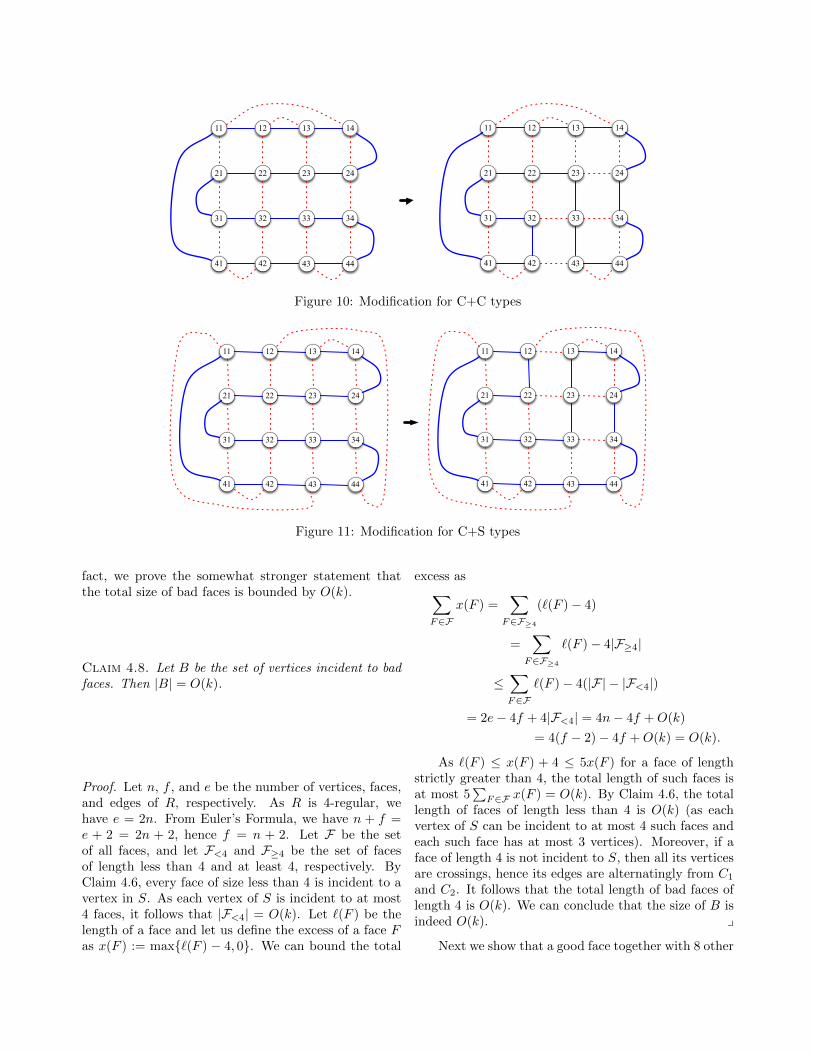
It remains only to show, for each of the typecombinations C+C, S+C, S+S, and S+(mirror imageof S), how the cycles are transformed. These are shownin Figures 10-13.

4.3 Bounding treewidth We show next that a rep-resentation not having a grid has treewidth O(

√k) and

then we use this to argue that the union of the two S-tours in Theorem 1.2 has bounded treewidth. Let usnote that we cannot obtain this bound by simply usingthe fact that a planar graph not containing a grid mi-nor has bounded treewidth. Our grid (see Figure 8a) isdefined as a subgraph, not as a minor, and moreover ithas the additional property that it is specified which ofthe edges come from which of the cycles.

Lemma 4.5. Consider a representation R =(G′, C1, C2) of (T1, T2) chosen to minimize the numberof vertices of the representation. If the representationcontains no grid, then its treewidth is O(

√k).

Proof. First, we observe some immediate consequencesof minimality.

Claim 4.6. Every face of length less than 4 is incidentto S.

Proof. Consider first a face F of length 2 not incidentto S (see Figure 14). The boundary of F contains

x1 y1

y2x2

x yF

x1 y1

y2x2

e1

e2w(x1x) + w(e1) + w(yy1)

w(x2x) + w(e2) + w(yy2)

Figure 14: Claim 4.6: eliminating a face of length 2.

one edge from each of C1 and C2: otherwise, therewould be a cycle of length 2 in C1 or C2. As Fis not incident to S, the two edges e1 ∈ E(C1) ande2 ∈ E(C2) of the face connect two vertices x, y 6∈ S,which are crossings by Prop. 4.1. Suppose that x1xyy1

is a subpath of C1 containing e1 and x2xyy2 is a subpathof C2 containing e2. We modify the representation byremoving both e1 and e2, adding an edge x1y1 of weightw(x1x) + w(e1) + w(yy1) to C1, and adding an edgex2y2 of weight w(x2x) + w(e2) + w(yy2) to C2. Fromthe fact that both x and y are crossings, it follows thatthe modified representation is also planar. The otherproperties of representations can be also verified easily.

Consider now a face F of length 3 not incidentto S. By Prop. 4.1, every vertex of F is a crossing.Therefore, the edges of F are alternatingly from C1 andC2, implying that the length of F cannot be odd. y

Claim 4.6 states that facial cycles of length less than 4intersect S, but this does not immediately imply thatthis is true for every cycle of length less than 4. Thefollowing claim proves this stronger statement.

Claim 4.7. Every cycle of length less than 4 containsa vertex of S.

Proof. Let C be a cycle of length less than 4. Let I bethe set of vertices strictly enclosed by C and let O be theset of vertices not enclosed by C. If I = ∅, then considera face enclosed by C. The vertices of this face are onC, thus it has at most 3 vertices and then Claim 4.6implies that C intersects S. Therefore, we can assumethat I is nonempty and, by a similar argument, that Ois nonempty. This means that each of C1 and C2 has atleast two edges between I and C, and between O andC. Thus the total degree of the vertices of C is at least2|C|+ 8 ≤ 4|C|, which contradicts |C| ≤ 3. y

We say that a face is good if it has length 4, no terminalis incident to it, and its boundary consists of edgesalternatingly from C1 and C2; otherwise, we say thatthe face is bad. We use Claim 4.6 and Euler’s Formulato give an O(k) bound on the number of bad faces; in

21 22 23

31 32 33

4241 43

24

34

44

11 12 13 14

21 22 23

31 32 33

4241 43

24

34

44

11 12 13 14

Figure 10: Modification for C+C types

21 22 23

31 32 33

4241 43

24

34

44

11 12 13 14

21 22 23

31 32 33

4241 43

24

34

44

11 12 13 14

Figure 11: Modification for C+S types

fact, we prove the somewhat stronger statement thatthe total size of bad faces is bounded by O(k).

Claim 4.8. Let B be the set of vertices incident to badfaces. Then |B| = O(k).

Proof. Let n, f , and e be the number of vertices, faces,and edges of R, respectively. As R is 4-regular, wehave e = 2n. From Euler’s Formula, we have n + f =e + 2 = 2n + 2, hence f = n + 2. Let F be the setof all faces, and let F<4 and F≥4 be the set of facesof length less than 4 and at least 4, respectively. ByClaim 4.6, every face of size less than 4 is incident to avertex in S. As each vertex of S is incident to at most4 faces, it follows that |F<4| = O(k). Let `(F ) be thelength of a face and let us define the excess of a face Fas x(F ) := max`(F ) − 4, 0. We can bound the total

excess as∑F∈F

x(F ) =∑

F∈F≥4

(`(F )− 4)

=∑

F∈F≥4

`(F )− 4|F≥4|

≤∑F∈F

`(F )− 4(|F| − |F<4|)

= 2e− 4f + 4|F<4| = 4n− 4f +O(k)

= 4(f − 2)− 4f +O(k) = O(k).

As `(F ) ≤ x(F ) + 4 ≤ 5x(F ) for a face of lengthstrictly greater than 4, the total length of such faces isat most 5

∑F∈F x(F ) = O(k). By Claim 4.6, the total

length of faces of length less than 4 is O(k) (as eachvertex of S can be incident to at most 4 such faces andeach such face has at most 3 vertices). Moreover, if aface of length 4 is not incident to S, then all its verticesare crossings, hence its edges are alternatingly from C1

and C2. It follows that the total length of bad faces oflength 4 is O(k). We can conclude that the size of B isindeed O(k). y

Next we show that a good face together with 8 other

21 22 23

31 32 33

4241 43

24

34

44

11 12 13 14

21 22 23

31 32 33

4241 43

24

34

44

11 12 13 14

Figure 12: Modification for S+S types

21 22 23

31 32 33

4241 43

24

34

44

11 12 13 14

21 22 23

31 32 33

4241 43

24

34

44

11 12 13 14

Figure 13: Modification for S+(mirror image of S) types

good faces surrounding it form a grid. While this soundsobvious, it requires a tedious case analysis to show thatthe vertices of the grid are distinct, and we need thetechnical condition that no 2-separator is present in theface.

Claim 4.9. Let F be a good face whose vertices do notcontain a 2-separator and are at distance at least 3 fromB. Then there is a grid.

Proof. Let the vertices of F be (2, 2), (2, 3), (3, 3), (3, 2)as in Figure 8a: the edge between (2, 2) and (2, 3) is fromC1, etc. We define (2, 1) as the neighbor of (2, 2) in C1

different from (2, 3), and define the vertices (1, 2), (1, 3),(2, 4), (3, 1), (3, 4), (4, 2), (4, 3) in a similar way. Notethat (2, 2) is a crossing by Proposition, thus the edgesincident to (2, 2) are indeed ordered as in Figure 8a.Furthermore, these vertices are not in B, hence areincident only to good faces. It follows that there isan edge of C2 between (2, 1) and (3, 1), an edge of C1

between (1, 2) and (1, 3), and so on. The vertices (1, 2),(2, 2), (2, 1) are part of a good face; we define (1, 1)

as the fourth vertex of that face. The vertices (1, 4),(4, 1), (4, 4) are defined similarly. By the way we definedthe vertices, any two vertices adjacent in Figure 8a areadjacent in R and each of the nine faces in Figure 8ais a face in R. However, we have to prove that all thedefined vertices are distinct.

We will be repeatedly using the following argument.Let C be any cycle of the representation and let I bethe set of vertices strictly enclosed by C. Let J1 and J2

be the subset of edges of C1 and C2, respectively, thatare between I and C. Then both |J1| and |J2| are even.

Let us define

X1 = (2, 2), (2, 3), (3, 2), (3, 3),X2 = (1, 2), (1, 3), (2, 1), (2, 4), (3, 1), (3, 4), (4, 2), (4, 3),X3 = (1, 1), (1, 4), (4, 1), (4, 4).

It is clear that the vertices of X1 are distinct. Let usshow that every vertex of X2 is distinct from the verticesinX1; by symmetry, it is sufficient to show this for (2, 1).We consider the following cases:

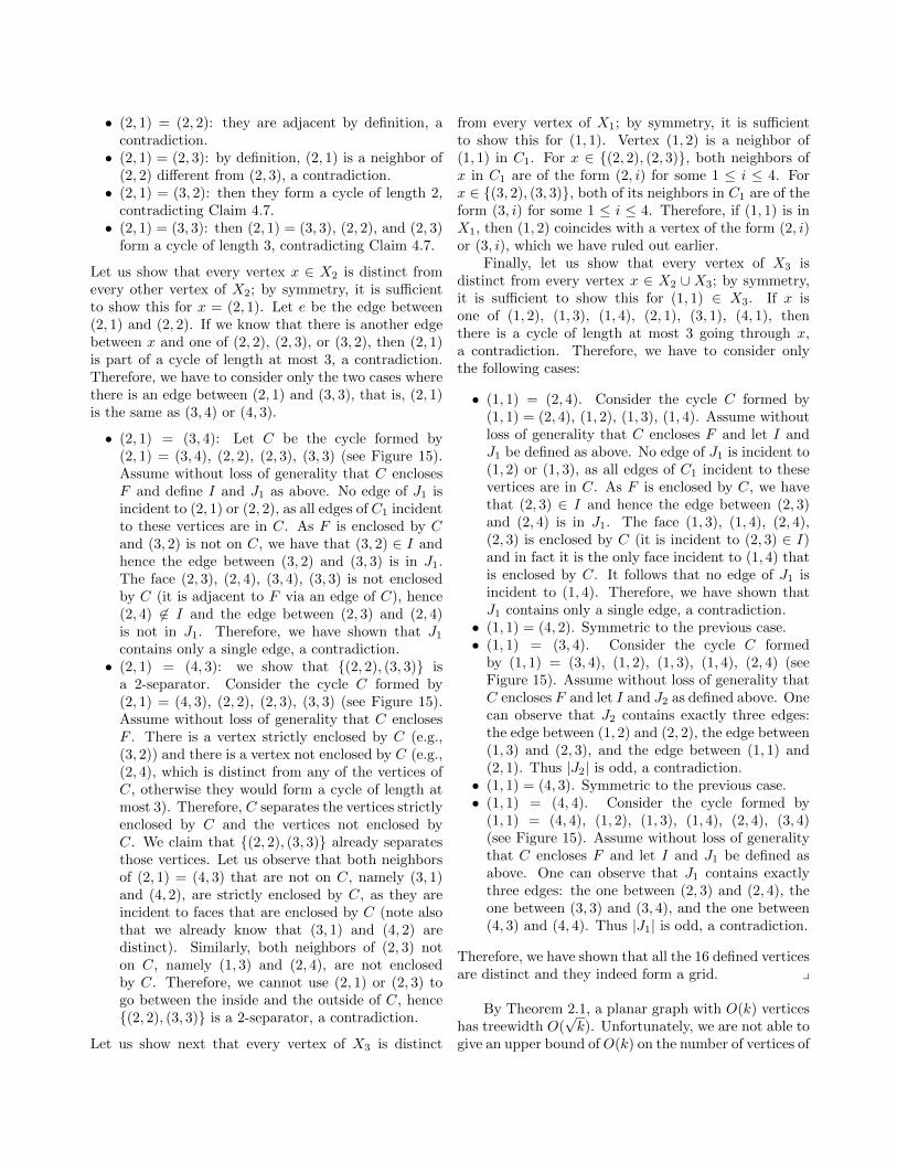
• (2, 1) = (2, 2): they are adjacent by definition, acontradiction.

• (2, 1) = (2, 3): by definition, (2, 1) is a neighbor of(2, 2) different from (2, 3), a contradiction.

• (2, 1) = (3, 2): then they form a cycle of length 2,contradicting Claim 4.7.

• (2, 1) = (3, 3): then (2, 1) = (3, 3), (2, 2), and (2, 3)form a cycle of length 3, contradicting Claim 4.7.

Let us show that every vertex x ∈ X2 is distinct fromevery other vertex of X2; by symmetry, it is sufficientto show this for x = (2, 1). Let e be the edge between(2, 1) and (2, 2). If we know that there is another edgebetween x and one of (2, 2), (2, 3), or (3, 2), then (2, 1)is part of a cycle of length at most 3, a contradiction.Therefore, we have to consider only the two cases wherethere is an edge between (2, 1) and (3, 3), that is, (2, 1)is the same as (3, 4) or (4, 3).

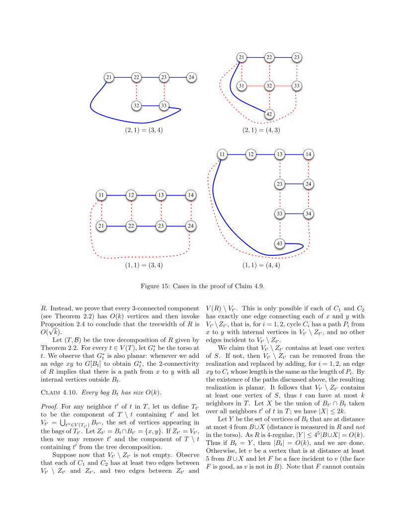
• (2, 1) = (3, 4): Let C be the cycle formed by(2, 1) = (3, 4), (2, 2), (2, 3), (3, 3) (see Figure 15).Assume without loss of generality that C enclosesF and define I and J1 as above. No edge of J1 isincident to (2, 1) or (2, 2), as all edges of C1 incidentto these vertices are in C. As F is enclosed by Cand (3, 2) is not on C, we have that (3, 2) ∈ I andhence the edge between (3, 2) and (3, 3) is in J1.The face (2, 3), (2, 4), (3, 4), (3, 3) is not enclosedby C (it is adjacent to F via an edge of C), hence(2, 4) 6∈ I and the edge between (2, 3) and (2, 4)is not in J1. Therefore, we have shown that J1

contains only a single edge, a contradiction.• (2, 1) = (4, 3): we show that (2, 2), (3, 3) is

a 2-separator. Consider the cycle C formed by(2, 1) = (4, 3), (2, 2), (2, 3), (3, 3) (see Figure 15).Assume without loss of generality that C enclosesF . There is a vertex strictly enclosed by C (e.g.,(3, 2)) and there is a vertex not enclosed by C (e.g.,(2, 4), which is distinct from any of the vertices ofC, otherwise they would form a cycle of length atmost 3). Therefore, C separates the vertices strictlyenclosed by C and the vertices not enclosed byC. We claim that (2, 2), (3, 3) already separatesthose vertices. Let us observe that both neighborsof (2, 1) = (4, 3) that are not on C, namely (3, 1)and (4, 2), are strictly enclosed by C, as they areincident to faces that are enclosed by C (note alsothat we already know that (3, 1) and (4, 2) aredistinct). Similarly, both neighbors of (2, 3) noton C, namely (1, 3) and (2, 4), are not enclosedby C. Therefore, we cannot use (2, 1) or (2, 3) togo between the inside and the outside of C, hence(2, 2), (3, 3) is a 2-separator, a contradiction.

Let us show next that every vertex of X3 is distinct

from every vertex of X1; by symmetry, it is sufficientto show this for (1, 1). Vertex (1, 2) is a neighbor of(1, 1) in C1. For x ∈ (2, 2), (2, 3), both neighbors ofx in C1 are of the form (2, i) for some 1 ≤ i ≤ 4. Forx ∈ (3, 2), (3, 3), both of its neighbors in C1 are of theform (3, i) for some 1 ≤ i ≤ 4. Therefore, if (1, 1) is inX1, then (1, 2) coincides with a vertex of the form (2, i)or (3, i), which we have ruled out earlier.

Finally, let us show that every vertex of X3 isdistinct from every vertex x ∈ X2 ∪ X3; by symmetry,it is sufficient to show this for (1, 1) ∈ X3. If x isone of (1, 2), (1, 3), (1, 4), (2, 1), (3, 1), (4, 1), thenthere is a cycle of length at most 3 going through x,a contradiction. Therefore, we have to consider onlythe following cases:

• (1, 1) = (2, 4). Consider the cycle C formed by(1, 1) = (2, 4), (1, 2), (1, 3), (1, 4). Assume withoutloss of generality that C encloses F and let I andJ1 be defined as above. No edge of J1 is incident to(1, 2) or (1, 3), as all edges of C1 incident to thesevertices are in C. As F is enclosed by C, we havethat (2, 3) ∈ I and hence the edge between (2, 3)and (2, 4) is in J1. The face (1, 3), (1, 4), (2, 4),(2, 3) is enclosed by C (it is incident to (2, 3) ∈ I)and in fact it is the only face incident to (1, 4) thatis enclosed by C. It follows that no edge of J1 isincident to (1, 4). Therefore, we have shown thatJ1 contains only a single edge, a contradiction.

• (1, 1) = (4, 2). Symmetric to the previous case.• (1, 1) = (3, 4). Consider the cycle C formed

by (1, 1) = (3, 4), (1, 2), (1, 3), (1, 4), (2, 4) (seeFigure 15). Assume without loss of generality thatC encloses F and let I and J2 as defined above. Onecan observe that J2 contains exactly three edges:the edge between (1, 2) and (2, 2), the edge between(1, 3) and (2, 3), and the edge between (1, 1) and(2, 1). Thus |J2| is odd, a contradiction.

• (1, 1) = (4, 3). Symmetric to the previous case.• (1, 1) = (4, 4). Consider the cycle formed by

(1, 1) = (4, 4), (1, 2), (1, 3), (1, 4), (2, 4), (3, 4)(see Figure 15). Assume without loss of generalitythat C encloses F and let I and J1 be defined asabove. One can observe that J1 contains exactlythree edges: the one between (2, 3) and (2, 4), theone between (3, 3) and (3, 4), and the one between(4, 3) and (4, 4). Thus |J1| is odd, a contradiction.

Therefore, we have shown that all the 16 defined verticesare distinct and they indeed form a grid. y

By Theorem 2.1, a planar graph with O(k) verticeshas treewidth O(

√k). Unfortunately, we are not able to

give an upper bound ofO(k) on the number of vertices of

21 22 23

32 33

24

21 22 23

31 32 33

42

(2, 1) = (3, 4) (2, 1) = (4, 3)

22 23 24

11 12 13 14

21

23

33

43

24

34

11 12 13 14

(1, 1) = (3, 4) (1, 1) = (4, 4)

Figure 15: Cases in the proof of Claim 4.9.

R. Instead, we prove that every 3-connected component(see Theorem 2.2) has O(k) vertices and then invokeProposition 2.4 to conclude that the treewidth of R isO(√k).Let (T,B) be the tree decomposition of R given by

Theorem 2.2. For every t ∈ V (T ), let G∗t be the torso att. We observe that G∗t is also planar: whenever we addan edge xy to G[Bt] to obtain G∗t , the 2-connectivityof R implies that there is a path from x to y with allinternal vertices outside Bt.

Claim 4.10. Every bag Bt has size O(k).

Proof. For any neighbor t′ of t in T , let us define Tt′

to be the component of T \ t containing t′ and letVt′ =

⋃t′′∈V (Tt′ )

Bt′′ , the set of vertices appearing in

the bags of Tt′ . Let Zt′ = Bt∩Bt′ = x, y. If Zt′ = Vt′ ,then we may remove t′ and the component of T \ tcontaining t′ from the tree decomposition.

Suppose now that Vt′ \ Zt′ is not empty. Observethat each of C1 and C2 has at least two edges betweenVt′ \ Zt′ and Zt′ , and two edges between Zt′ and

V (R) \ Vt′ . This is only possible if each of C1 and C2

has exactly one edge connecting each of x and y withVt′ \Zt′ , that is, for i = 1, 2, cycle Ci has a path Pi fromx to y with internal vertices in Vt′ \ Zt′ , and no otheredges incident to Vt′ \ Zt′ .

We claim that Vt′ \ Zt′ contains at least one vertexof S. If not, then Vt′ \ Zt′ can be removed from therealization and replaced by adding, for i = 1, 2, an edgexy to Ci whose length is the same as the length of Pi. Bythe existence of the paths discussed above, the resultingrealization is planar. It follows that Vt′ \ Zt′ containsat least one vertex of S, thus t can have at most kneighbors in T . Let X be the union of Bt′ ∩ Bt takenover all neighbors t′ of t in T ; we have |X| ≤ 2k.

Let Y be the set of vertices of Bt that are at distanceat most 4 from B∪X (distance is measured in R and notin the torso). As R is 4-regular, |Y | ≤ 45|B∪X| = O(k).Thus if Bt = Y , then |Bt| = O(k), and we are done.Otherwise, let v be a vertex that is at distance at least5 from B∪X and let F be a face incident to v (the faceF is good, as v is not in B). Note that F cannot contain

a 2-separator: by the remark after Theorem 2.2, the 2-separators are of the form Bt′ ∩ Bt′′ for two distinctnodes t′ and t′′, i.e., they have to contain vertices frombags other than Bt and all such vertices are in X.Therefore, the conditions of Claim 4.9 hold, and thereexists a grid, a contradiction. y

Finally, we can complete the proof of Lemma 4.5.By Claim 4.10, every bag has size O(k). As every torsoG∗t is planar, Theorem 2.1 implies that every torso G∗thas treewidth O(

√k). By Proposition 2.4, it follows

that R has treewidth O(√k).

Now we are ready to prove the main combinatorialresult, Theorem 1.2.

Proof. of Theorem 1.2. Let us invoke Lemma 4.4 onthe metric d and the 4-opt solution T4; let Topt bethe resulting optimal solution and (G′, C ′1, C

′2) be the

minimal representation of (T4, Topt) containing no grid.

By Lemma 4.5, the treewidth of G′ is O(√k).

We construct a graph G′′ from G′ by replacing eachvertex v ∈ V (G′) with two adjacent vertices v1, v2,and for every edge xy ∈ E(G′), we make every vertexin x1, x2 adjacent to every vertex in y1, y2. IfG′ has a tree decomposition of width w − 1 (that is,maximum bag size w), then it is clear that G′′ has atree decomposition of width 2w − 1 (that is, maximumbag size 2w). Therefore, the treewidth of G′′ is alsoO(√k).We claim that T4 ∪ Topt is a minor of G′′, hence

the treewidth bound of O(√k) follows also for T4∪Topt.

We define the cycle C ′′4 by replacing every v ∈ V (C4)with v1. We define cycle C ′′opt by replacing every v ∈V (Copt) \ S with v2 and replacing every v ∈ S with v1.Now it is easy to see that C ′′4 ∪ C ′′opt is a subdivision ofT4 ∪ Topt, hence T4 ∪ Topt is a minor of G′′.

References

[1] S. Arora. Polynomial-time approximation schemes forEuclidean TSP and other geometric problems. Journalof the ACM, 45(5):753–782, 1998.

[2] S. Arora, M. Grigni, D. R. Karger, P. N. Klein,and A. Woloszyn. A polynomial-time approximationscheme for weighted planar graph TSP. In Proceedingsof the 9th Annual ACM-SIAM Symposium on DiscreteAlgorithms, pages 33–41, 1998.

[3] A. Atserias, A. A. Bulatov, and V. Dalmau. On thepower of k-consistency. In ICALP, pages 279–290,2007.

[4] R. Bellman. Dynamic programming treatment of thetravelling salesman problem. J. ACM, 9(1):61–63, Jan.1962.

[5] A. Bjorklund, T. Husfeldt, P. Kaski, and M. Koivisto.The travelling salesman problem in bounded degreegraphs. In L. Aceto, I. Damgrd, L. Goldberg, M. Hall-drsson, A. Inglfsdttir, and I. Walukiewicz, editors, Au-tomata, Languages and Programming, volume 5125 ofLecture Notes in Computer Science, pages 198–209.Springer Berlin Heidelberg, 2008.

[6] H. Chen and V. Dalmau. Beyond hypertree width:Decomposition methods without decompositions. InCP, pages 167–181, 2005.

[7] N. Christofides. Worst-case analysis of a new heuristicfor the travelling salesman problem. Technical Report388, Graduate School of Industrial Administration,Carnegie Mellon University, 1976.

[8] W. Cook and P. D. Seymour. Tour merging via branch-decomposition. INFORMS Journal on Computing,15(3):233–248, 2003.

[9] E. D. Demaine, F. V. Fomin, M. T. Hajiaghayi,and D. M. Thilikos. Subexponential parameterizedalgorithms on bounded-genus graphs and h-minor-freegraphs. J. ACM, 52(6):866–893, 2005.

[10] E. D. Demaine and M. Hajiaghayi. The bidimension-ality theory and its algorithmic applications. Comput.J., 51(3):292–302, 2008.

[11] R. Diestel. Graph Theory, 4th Edition, volume 173 ofGraduate texts in mathematics. Springer, 2012.

[12] F. Dorn, E. Penninkx, H. L. Bodlaender, and F. V.Fomin. Efficient exact algorithms on planar graphs:Exploiting sphere cut decompositions. Algorithmica,58(3):790–810, 2010.

[13] D. Eppstein. The traveling salesman problem forcubic graphs. In F. Dehne, J.-R. Sack, and M. Smid,editors, Algorithms and Data Structures, volume 2748of Lecture Notes in Computer Science, pages 307–318.Springer Berlin Heidelberg, 2003.

[14] H. Gebauer. Enumerating all Hamilton cycles andbounding the number of Hamilton cycles in 3-regulargraphs. Electr. J. Comb., 18(1), 2011.

[15] M. Grigni, E. Koutsoupias, and C. H. Papadimitriou.An approximation scheme for planar graph TSP. InFOCS, pages 640–645, 1995.

[16] M. Grohe. Fixed-point definability and polynomialtime on graphs with excluded minors. J. ACM,59(5):27:1–27:64, Nov. 2012.

[17] M. Held and R. Karp. The traveling-salesman problemand minimum spanning trees: Part II. MathematicalProgramming, 1(1):6–25, 1971.

[18] K. Iwama and T. Nakashima. An improved exactalgorithm for cubic graph TSP. In G. Lin, editor,Computing and Combinatorics, volume 4598 of LectureNotes in Computer Science, pages 108–117. SpringerBerlin Heidelberg, 2007.

[19] D. S. Johnson and L. A. McGeoch. The travelingsalesman problem: A case study in local optimization.In E. Aarts and J. Lenstra, editors, Local searchin combinatorial optimization, pages 215–310. Wiley,1997.

[20] D. Karapetyan and G. Gutin. Lin-Kernighan heuris-

tic adaptations for the generalized traveling salesmanproblem. European Journal of Operational Research,208(3):221–232, 2011.

[21] D. Karapetyan and G. Gutin. Efficient local searchalgorithms for known and new neighborhoods for thegeneralized traveling salesman problem. EuropeanJournal of Operational Research, 219(2):234–251, 2012.

[22] P. N. Klein. A linear-time approximation scheme forplanar weighted TSP. In FOCS, pages 647–657, 2005.

[23] P. N. Klein. A subset spanner for planar graphs, withapplication to subset TSP. In STOC, pages 749–756,2006.

[24] P. N. Klein. A linear-time approximation scheme forTSP in undirected planar graphs with edge-weights.SIAM Journal on Computing, 37(6):1926–1952, 2008.

[25] T. Kloks. Treewidth, volume 842 of Lecture Notes inComputer Science. Springer, Berlin, 1994.

[26] S. Lin and B. W. Kernighan. An effective heuristicalgorithm for the traveling-salesman problem. Opera-tions Research, 21(2):pp. 498–516, 1973.

[27] D. Lokshtanov, D. Marx, and S. Saurabh. Lowerbounds based on the Exponential Time Hypothesis.Bulletin of the EATCS, 105:41–72, 2011.

[28] D. Marx. Searching the k-change neighborhood forTSP is W[1]-hard. Oper. Res. Lett., 36(1):31–36, 2008.

[29] J. Mitchell. Guillotine subdivisions approximatepolygonal subdivisions: Part ii – a simple PTAS forgeometric k-MST, TSP, and related problems. SIAMJournal on Computing, 28:298–1309, 1999.

[30] S. Rao and W. Smith. Approximating geometricalgraphs via “spanners” and “banyans”. In Proceedingsof the 30th Annual ACM Symposium on the Theory ofComputing, pages 540–550, 1998.

[31] N. Robertson, P. D. Seymour, and R. Thomas. Quicklyexcluding a planar graph. J. Comb. Theory, Ser. B,62(2):323–348, 1994.

[32] W. D. Smith and N. C. Wormald. Geometric sepa-rator theorems & applications. In Proceedings of the39th Annual Symposium on Foundations of ComputerScience, pages 232–243, 1998.