a study on the effects of soft interference 1 jun 2 1 20
TRANSCRIPT
A Study on the Effects of Soft Interference 1 JUN 2 1 20Cancellation for Uplink WCDMA system
byL1BEPRIETianren Qi
Submitted to the Department of Electrical Engineering and ComputerScience ARCHIVES
in partial fulfillment of the requirements for the degree ofMasters of Engineering in Electrical Engineering and Computer
Scienceat the
MASSACHUSETTS INSTITUTE OF TECHNOLOGYJune 2011
@ Massachusetts Institute of Technology 2011. All rights reserved.
Author .................................... ...........Department of Electrical Engineering and Computer Science
May 18, 2011
Certified by............Y Liz ong Zheng
Associate P fessor, MITM.I, T sis Supervisor
Certified by.......Mingxi Fan
Senior Director of Engineering, QualcommVI-A Company Thesis Supervisor
Certified by. ..................Yisheng Xue
Senior Staff Engineer/Manager. QualcommVI-A Company Co-Thesis Supervisor
Certified by............ .......Jiye Liang
Senior Engineer, QualcommVI-A Company Thesidnane
Accepted by .......................Dr. unistopnerJ. ierman
Chairman, Masters of Engineering Thesis Committee


A Study on the Effects of Soft Interference Cancellation for
Uplink WCDMA system
by
Tianren Qi
Submitted to the Department of Electrical Engineering and Computer Scienceon May 18, 2011, in partial fulfillment of the
requirements for the degree ofMasters of Engineering in Electrical Engineering and Computer Science
Abstract
WCDMA system is an interference limited system. Interference cancellation (IC) is atechnique that has been widely studied and implemented for WCDMA uplink systemto achieve performance close to potential capacity. Most studies until now have beenfocused on hard interference cancellation. Hard IC occurs after each user has itscyclic redundancy check (CRC) passed, meaning it would not perform cancellationuntil the end of a transmission time interval(TTI), therefore causing potential delaysin cancellation. Recently engineers have proposed a soft IC scheme where one wouldperform cancellation without passing CRC, therefore one would not have as muchdelay on cancellation but at the cost of lower cancellation efficiency because of badestimation on signals. In my thesis I will attempt to build a framework that givessome insight to the tradeoff between hard and soft IC to serve as a reference forengineers when implementing IC into our WCDMA systems.
M.I.T Thesis Supervisor: Lizhong ZhengTitle: Associate Professor, MIT
VI-A Company Thesis Supervisor: Mingxi FanTitle: Senior Director of Engineering, Qualcomm
VI-A Company Co-Thesis Supervisor: Yisheng XueTitle: Senior Staff Engineer/Manager, Qualcomm
VI-A Company Co-Thesis Supervisor: Jiye LiangTitle: Senior Engineer, Qualcomm

4

Acknowledgments
It is a pleasure to thank those who made this thesis possible. First I am grateful to
my director at Qualcomm, Dr. MIngxi Fan who provided me the opportunity to work
on the project, and also the constant support and insight in the overall direction on
my thesis.
I want to thank Dr. Jiye Liang and Dr. Yisheng Xue for the greatest mentorship I
ever had and always be there to answer all my questions.
I want to thank my on campus supervisor Professor Lizhong Zheng who gratefully
accepted the duty as my thesis supervisor and helped me on the formatting of the
thesis.
I would also like to thank the entire Qualcomm China team for been extremely helpful
colleagues and giving me a nice scope of the entire wireless communication industry.
Lastly thanks go to my family and friends for supporting me for the past 21 years.

6

Contents
1 Introduction
1.1 Background . . . . . . . . . . . . . .
1.2 Problem Approach . . . . . . . . . .
2 Hard IC Without Early Termination
2.1 Problem Setup . .
2.2 Baseline . . . . . .
2.2.1 Derivations
2.2.2 Results.
2.3 Hard Pilot IC .
2.3.1 Derivation
2.3.2 Results .
2.4 Hard Traffic IC
2.4.1 Derivation
2.4.2 Results . . .
2.5 Hard TIC+PIC . .
2.5.1 Derivations
2.5.2 Results . . .
3 Hard IC with Early Termination
3.1 Early Termination Concepts .
3.2 Baseline Early Termination .
3.2.1 Derivation .........
21
. . . . . . . . . . . . 21
. . . . . . . . . . . . 25
. . . . . . . . . . . . 25
. . . . . . . . . . . . 26
. . . . . . . . . . . . 27
. . . . . . . . . . . . 27
. . . . . . . . . . . . 29
. . . . . . . . . . . . 30
. . . . . . . . . . . . 30
. . . . . . . . . . . . 34
. . . . . . . . . . . . 35
. . . . . . . . . . . . 35
. . . . . . . . . . . . 37
39
39
41
41
. . . . . . . . . . . . . . . .
. . . . . . . . . . . . . . . .
. . . . . . . . . . .
. . . . . . . . . . .
. . . . . . . . . . .
. . . . . . . . . . .
. . . . . . . . . . .
. . . . . . . . . . .
. . . . . . . . . . .
. . . . . . . . . . .
. . . . . . . . . . .
. . . . . . . . . . .
. . . . . . . . . . .
. . . . . . . . . . .
. . . . . . . . . . .
. . . . . . . . . . . . . . . . . . .
. . . . . . . . . . . . . . . . . . .
. . . . . . . . . . . . . . . . . . .

3.2.2 Results . . . . . . . . . . . . . . . . . . . . . . . . . . . . . . . 43
3.3 Hard IC with early termination . . . . . . . . . . . . . . . . . . . . . 43
3.3.1 Derivation . . . . . . . . . . . . . . . . . . . . . . . . . . . . . 43
4 Soft IC 53
4.1 Problem Setup . . . . . . . . . . . . . . . . . . . . . . . . . . . . . . 54
4.2 Symbol Level Cancellation . . . . . . . . . . . . . . . . . . . . . . . . 57
4.3 Soft IC every half of a TTI . . . . . . . . . . . . . . . . . . . . . . . . 58
4.4 Results and Qualitative Analysis . . . . . . . . . . . . . . . . . . . . 60
5 Conclusion and possible future work 63
List of Figures
1-1 WCDMA Timing ....... ............................. 15
1-2 Uplink WCDMA system ...... ......................... 16
1-3 A brief uplink physical layer procedure .... ................. 18
2-1 A general diagram for WCDMA system where data are divided into
pilot channel and traffic channel . . . . . . . . . . . . . . . . . . . . . 23
2-2 A diagram representing how PIC works . . . . . . . . . . . . . . . . . 28
2-3 PIC effective RoT calculation . . . . . . . . . . . . . . . . . . . . . . 29
2-4 A diagram showing how TIC works with user i's perspective ..... 31
2-5 A diagram showing how TIC works with user l's perspective . . . . . 32
2-6 3 users RoT calculated when viewing from slot 1 . . . . . . . . . . . . 33
2-7 3 users RoT calculated when viewing from slot 3 . . . . . . . . . . . . 34
3-1 Baseline early termination . . . . . . . . . . . . . . . . . . . . . . . . 42
3-2 Baseline early termination . . . . . . . . . . . . . . . . . . . . . . . . 42
3-3 Plot of effective RoT against the probability of early termination . . . 44
3-4 Plot of system capacity (number of users) against the probability of
early termination . . . . . . . . . . . . . . . . . . . . . . . . . . . . . 44
3-5 Demonstration of early termination with interference cancellation from
user l's perspective . . . . . . . . . . . . . . . . . . . . . . . . . . . . 46
3-6 Demonstration of early termination with interference cancellation from
user k's perspective . . . . . . . . . . . . . . . . . . . . . . . . . . . . 47
3-7 Case 1 of effective RoT calculation . . . . . . . . . . . . . . . . . . . 50
3-8 Case 2 of effective RoT calculation . . . . . . . . . . . . . . . . . . . 50

3-9 Case 3 of effective RoT calculation . . . . . . . . . . . . . . . . . . . 50
4-1 Pre-decoding Soft Interference Cancellation Demonstration . . . . . . 56
4-2 Symbol level cancellation . . . . . . . . . . . . . . . . . . . . . . . . . 57
4-3 Post Decoding Soft IC . . . . . . . . . . . . . . . . . . . . . . . . . . 59
4-4 Soft IC every 15 slots . . . . . . . . . . . . . . . . . . . . . . . . . . . 60
10

List of Tables
2.1 Baseline results . . . .
2.2 Hard PIC only results
2.3 Hard TIC only results
2.4 Hard TIC+PIC results
..........................
..........................
..........................
..........................

12

Chapter 1
Introduction
1.1 Background
Standing for wideband code division multiple access, WCDMA is one of the most
commonly used wireless communication system in the world. Unlike previous tech-
nologies, WCDMA systems allow users to transmit data at the same time under the
same frequencies. This technology allows a greater user capacity but it is limited by
the amount of interference each user sees. In this thesis we will explore some effects
of interference cancellation.
I will first introduce some background about WCDMA. In this thesis we will
specifically focus on uplink WCDMA system. The system is modeled as follows: we
have many users (one can think them as operating cellphones in the region), each of
them is transmitting data to the base station (one can think it as cellphone towers)
to process, and we are interested in how can the base station process the data in a
most efficient and accurate way.
First we see that the single most important concept in WCDMA system is SINR,
standing for signal to interference and noise ratio. This ratio tells us how clear our
received data is for each individual user, meaning the ratio between each user's power
against the overall power used in the system. To put this as an analogy, we can
imagine a room full of people talking. In order for person A to hear person B, person
B must talk loud enough, or as a fraction of how loud everyone else are, in order for

person A to be able to hear person B. To compare this WCDMA system with our
analogy more, we can imagine that in order for one person to clearly deliver his mes-
sage to another, he needs to talk in sentences, meaning he will try to group his words
and deliver the message piece by piece. This is done in WCDMA system through the
implementation of transmission time interval (TTI). Each TTI is 10 milliseconds to
80 milliseconds. The base station will try to decode (understand) TTI by TTI, and
after the base station is done with everyone's transmitted TTI, it will move on to the
next TTI.
In fact each TTI can be broken down into subparts too. Following diagram 1-1,
we see that each TTI can be broken down to a number of slots, and each slot is
consisted of a number of symbols. Following [5], we know that each user transmits
symbol by symbol to the base station by the following procedure:
In a basic k users channel model, if we assume each user's symbol arrives syn-
chronously, then what the base station (or Node-B) receives is the following waveform:
k
g= - Ai bisi + an'o(1)i=1
Ai represents the received amplitude of the ith user's signal, meaning that A.
is the power transmitted by the ith user. bi is the bit transmitted by the ith user.
s is a signature that has unit energy and it's a deterministic waveform assigned to
each specific user i. si is known to base station so when the base station wants to
extract user i's signal, it will take the dot product of si and p. no is the Gaussian
background noise with unit power spectral density. It models thermal noise plus
other noise sources unrelated to the transmitted signals. Theoretically if each user's
signature is orthogonal to each other, meaning that |(si, s) = 0 for user i and j,then the clarity of the symbol we extracted only depends on the signal to noise ratio,
namely As/o-, but because of channel fading and other reasons, we can not have the
signatures for different users to be perfectly orthogonal, therefore the performance
depends on |(si, S-) I as well. So all these inter-symbol correlation leads to our interest
in interference.
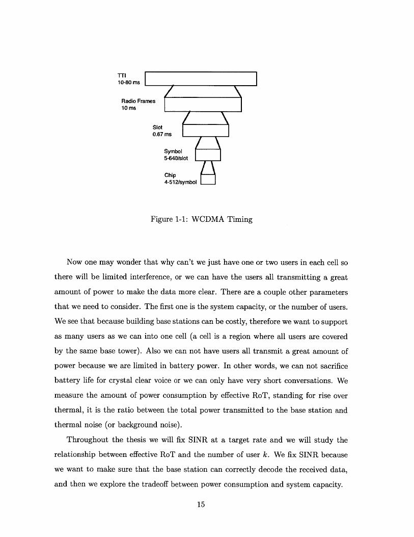
TTI10-80 ms
Radio Frames10 ms
Slot0.67 ms
Symbol5-640/slot
Chip4-512/symbol
Figure 1-1: WCDMA Timing
Now one may wonder that why can't we just have one or two users in each cell so
there will be limited interference, or we can have the users all transmitting a great
amount of power to make the data more clear. There are a couple other parameters
that we need to consider. The first one is the system capacity, or the number of users.
We see that because building base stations can be costly, therefore we want to support
as many users as we can into one cell (a cell is a region where all users are covered
by the same base tower). Also we can not have users all transmit a great amount of
power because we are limited in battery power. In other words, we can not sacrifice
battery life for crystal clear voice or we can only have very short conversations. We
measure the amount of power consumption by effective RoT, standing for rise over
thermal, it is the ratio between the total power transmitted to the base station and
thermal noise (or background noise).
Throughout the thesis we will fix SINR at a target rate and we will study the
relationship between effective RoT and the number of user k. We fix SINR because
we want to make sure that the base station can correctly decode the received data,
and then we explore the tradeoff between power consumption and system capacity.

Other cells that support
Base Station users near it
(Node-B)
Individual userstransmitting signals
Figure 1-2: Uplink WCDMA system
Now we will discuss some background and motivation of the work presented in this
thesis. As the title states, we want to study the effect of the different implementations
of interference cancellation. From [1], in a general view, We see that if we let P and
Ri be the power and rate user i is transmitting respectively, and background noise
as No, from Shannon theory we have that R, <; log 2(1 + Pi ). In the case ofNo+ E Pk
k#i
very large k, we see that E Pk decreases proportionally with k, so ln(1 + x) ~ x -+
k3i
log2 (1 + X) ~ x/ In 2 and this gives us the total rate that users can transmit at:
k k
Rtotai < - EZ' i(1.2)1 n 2 _1 No + Pk
kAi
But then if we study the theoretical sum rate capacity of a WCDMA system, we
have that capacity C is equal to log 2 (1 + ). So we see that this is significantly
a better bound than the bound presented in 1.2. We see that the difference between
two bound is that in 1.2, the term [ Pk is significantly reducing the system capac-k~j

ity, so that if we can reduce the amount of interference seen, we can achieve better
performance.
We will now discuss interference cancellation from a top view. From [5] and [7],
there are three categories of cancellation schemes: successive interference cancella-
tion, parallel interference cancellation, and group interference cancellation. In this
thesis we will mainly focus on successive interference cancellation (SIC) and parallel
interference cancellation. From a top view how base station cancels interference is as
follows: first it will save all the currently transmitted signals (usually by the length
of TTI) into a buffer, then it will try to decode the received signals. After that the
base station will try to reconstruct the received signals and subtract the reconstructed
signals from the buffer. In SIC users are ordered by their arrival time at the base
station and the first user is decoded first. Upon successful decoding, the signal is
reconstructed and cancelled from the buffer. In parallel interference cancellation, all
the users' signals will be estimated at the same time, and after all the estimations are
done the base station will reconstruct the signals and cancel them.
Now we see the importance of SINR and reducing interference seen by users, we
will make introductions to a different way to categorize interference cancellation. In
this paper we will discuss hard interference cancellation (hard IC), soft interference
cancellation (soft IC), and early termination (ET).
In WCDMA system, interference is usually cancelled by the base station recon-
structing signals it received and subtract the reconstructed signals from its buffer.
IC can be categorized in two ways depending on a cyclic redundancy check (CRC).
Usually data are transmitted in the following ways: first the user will obtain the data
it tries to send, then it will add a piece of code that is known to both users and the
base station to the end of the data. The users will follow the procedure on diagram
1-3 to send its data and CRC. At the base station, one will try to first demodulate the
received data and despread them, then it will turbo decode the data and finally it will
try to match the decoded data against the known CRC bits. In [2], engineers have
proposed a method to reconstruct data and add back to communication channel after
CRC passed, and this interference cancellation method is known as "post CRC IC,"

Figure 1-3: A brief uplink physical layer procedure
or hard interference cancellation. In [1], engineers proposed an IC algorithm where
we use the soft output from turbo decoder to make symbol estimation, this is called
"post decoding soft IC." We see that soft output from the turbo decoder does not
depend on the successfulness of decoding. Also in [3], engineers proposed another IC
scheme where the base station will try to estimate symbols right after demodulation
without the output of turbo decoding. This means that we will reconstruct signals
before turbo decoding. So this method is known as "pre decoding soft IC." One can
see that in soft interference cancellation, base station reconstruct the signals quicker
because it does not need to decode, but it may not be as accurate because we recon-
struct our signals before passing the signal to turbo decoder. In the extreme case we
see that subtracting inaccurate reconstructed signals can worsen the system because
we might be simply adding more interference into the channel. So for most part of
the thesis we will study the trade off between delaying in application of interference
cancellation and accuracy of interference cancellation.
Now we will talk about early termination (ET). ET is another method that
WCDMA system uses to reduce interference. How ET works is as follows: instead of

the base station trying to decode the received signals after users have done transmit-
ting, the base station will try to decode once it starts to receive data. Because we
are using turbo coding, we see that there are many redundancy in our transmitted
data, therefore if the base station gets the correct piece of data, it can finish decod-
ing before the users finish transmitting. So the base station can tell the users to
stop transmitting in that case therefore we have less transmission which lead to less
interference.
1.2 Problem Approach
We see that even though previous engineers have proposed different interference can-
cellation algorithms and did a lot of real world simulations to their proposed algo-
rithms, but one lack a general model that study the different effects of interference
cancellation. So in this thesis we will try to understand interference cancellation from
an abstract level.
We see that engineers have done simulations to study hard IC, and the results
of the simulation is presented in table 2.1, 2.2, 2.3, and 2.4. But engineers have not
generalized their simulation results to soft IC or early termination or any combination
of early termination and interference cancellation. Therefore this thesis will try to
build a model that will give generalized results regarding soft IC and ET. To prove
that the model is reasonable, we will first check the results of the model in hard IC
scenario against simulation results. If the model and simulation are within a close
range of each other, we conclude that the problem approach is correct, therefore we
will recommend future engineers to use the generalized model presented in later parts
of the thesis when evaluating performance of ET and soft IC. This will save time for
others to not conducting more simulations regarding ET and soft IC.
Now I will give a detailed breakdown of what the thesis is going to cover:
Chapter 2: At the beginning of the chapter we will give the general problem set
up. And then for most part of this chapter we will study the effect of hard interference
cancellation. The work in this chapter will serve as the control check of our thesis
because we have real world simulation results provided. The simulation results are
provided by Qualcomm engineers who have conducted research in hard interference
cancellation. We will trust the simulation results since for the past engineers have
shown that the simulation is an accurate approximation of real world situations. So
for this chapter we will check our derived results against the simulation, and if the
results match with simulation, we can conclude that our general problem approach is
reasonable, enable us to move on to later chapters.
Chapter 3: In this chapter we will study the effect of early termination. We will
explain how early termination works in detail and state some of the assumptions in
the derivation. Then we will combine the results of basic early termination results
with hard interference cancellation and explore how early termination helps the sys-
tem performance.
Chapter 4: In this chapter we will combine the results of early termination and
hard interference cancellation to study how well soft interference cancellation have to
do in order to out perform hard interference cancellation. Two schemes of soft inter-
ference cancellation will be presented. The first one is a pre-decoding soft IC scheme
where one would make symbol estimations just based on the output of demodulation.
The second is a post-decoding soft IC scheme where one will make estimations of
received signals based on the soft output from turbo decoder. We will make some
general conclusions about different schemes of soft interference cancellation. We will
present this results to the engineers so they can have more reference in regard of which
interference cancellation scheme to implement into our current WCDMA system.
Chapter 5: We will discuss what possible future study we can do regarding soft
interference cancellation. We will also discuss what other results we may need in
order for engineers to make better decisions.

Chapter 2
Hard IC Without Early
Termination
As described in the introduction, we will explore hard interference cancellation in this
chapter. We measure the difference between algorithms of interference cancellation
by holding Signal to Interference and Noise ratio (SINR) constant and explore the
different gains in system capacity and power efficiency. Also at the end of each
section, we would like to compare our results against simulations. The simulations are
provided by Qualcomm engineers and they have shown that the simulation matches
well against real world scenarios. If our derivations for this section are consistent with
the existing simulation results, we can conclude that the problem setup is correct.
2.1 Problem Setup
Before we dig into the detailed calculation, a few assumptions and definitions must
be made about the model. First we have to discuss different sources of interference.
Generally we have three sources: intra-cell, inter-cell, and self. Intra-cell interference
is defined as the interference contributed from a user within the cell. Inter-cell in-
terference is the interference from other cells, and self interference is the interference
from itself due to multi-path effect.
We assume that we have all cells running the same algorithms. This means that

we will model inter-cell interference as a constant ratio compared to intra-cell inter-
ference. This is a reasonable assumption because consider we are running the same
model in every cell, we see that each cell's intra-cell interference can be approximated
as the same, therefore the only factor affecting inter and intra cell interference is the
distance from the base station in our interested cell, which we can treat as a constant
factor from the inter-cell interference. We see that applying interference cancellation
does not affect our assumptions either, because in our derivation we will not consid-
ering apply interference cancellation to other cells. We simply calculate the desired
power one should transmit to maintain SINR, and then we regard inter-cell interfer-
ence simply as a factor multiplied by the sum of the power transmitted in this cell
before interference cancellation applied. We are also only using a single rake receiver
at the base station so in the derivation we ignore the interference due to multi-path
fading, meaning that we do not consider self interference. These assumptions can be
sources of error when comparing theoretical and simulation results.
The last important assumption is that in this WCDMA uplink model we assume
that our communication channel is composed of two parts: pilot channel and traffic
channel. All users will transmit a known sequence of bits in the pilot channel, there-
fore we can assume that the base station will decode all the pilot channel at the same
time (following parallel IC's framework). The purpose of transmitting a sequence of
known bits in pilot channel before transmitting actual data in traffic channel is be-
cause the base station wants to have a good channel estimation before start decoding.
For the ease of calculation, we have k, be the number of users transmitting in pilot
channel and kt be the number of users transmitting in traffic channel. In simulation
though, we assume that kt = k, to make calculation even more easy. Also to make
notations easier to observe, we let At {a } be the set of indices of users who are
transmitting signals in the traffic channel, and As,, = {b3} be the set of indices of users
who are transmitting signals in the pilot channel. So we have:
|At|= kt and |AI= k, (2.1)

Pilot Channel
Traffic Channel
user 1'
user2'
user kp
user 1user 2
user k
Key: The shaded region represents the current TTI that we are trying to decode
Figure 2-1: A general diagram for WCDMA system where data are divided into pilotchannel and traffic channel
For the traffic channel, we assume that the base station will decode each user
in the order they are received, and we assume an asynchronous frame for the traffic
channel. We know from [5] and [2] in an asynchronous framework users signals will
arrive uniformly distributed within the TTI, so for rest of the thesis in order to make
the calculation easier, we assume each user arrives at a fixed time and the arrival
time is spaced evenly across each TTI. Also we assume that we have a relatively long
time of transmission; we are in the middle of a long sequence of TTI's therefore we
see that we are in the situation in the following diagram 2-1.
Now we will define a few terms that are essential throughout the derivation. The
first one is the total power transmitted by user i in a TTI, we denote this as Eci.
We see that each user transmit through both pilot and traffic channel, therefore
Eci = Ed,j + Ee,, where Et,i is the power transmitted through the traffic channel
and Eep,i is the power transmitted through the pilot channel. Usually we are given a
traffic to pilot ratio, denoted by T/P, which represents the ratio between each user's
power transmission through the traffic channel and pilot channel. T/P is fixed and

constant throughout our derivation and simulation.
We will give more definitions regarding interference. When the base station is de-
coding, it sees three sources of interference: thermal noise, inter-cell interference and
intra-cell interference. We denote thermal noise as No since it is usually a normally
distributed white noise in the background. We will also define f as the inter-cell
interference to intra-cell interference ratio. Because we only apply interference can-
cellation within the cell, so we want inter-cell interference to be a constant. Therefore
we have:
F = f -Io = total inter-cell interference (2.2)
Then we define the total intra-cell interference seen in a cell as Io. So in the case
where no interference cancellation is applied:
10 = 1 Ect,j + 1 Ecp,j (2.3)iEAt jEAp
We see that Io is simply the sum of all the power of signals transmitted in traffic
and pilot channel. Because previously we assumed that we will ignore self-interference,
we will deduct the power of the user from the total interference defined above. So we
define SINR:
SINR traffic power Ect,jNoise+Interference Io + F + No - Ec,
Ect,j (2.4)
No + F + ( Ectjg + ( Ec,,jEAt LcAp
We can also relate SINR and Io + F + No. Because in simulation we are only
given the Io+EFNo ratio, we need to somehow relate Io + F + No and SINR to find a
numerical value of the SINR that we are going to fix constant for rest of the thesis.
Also with the definition of T/P we have that Ec, = Ec,,i -T/P = I Ec,, and

similarly Ecp,i = Ec,. We see that:
T/P
NR Ect, 1 1 1+T/P
Io+F+No-Eci Ip+F+No _ _ - 1+T/P 1' Ec:t,j Ect,j TIP10 NO~ TI+ ONOI~ T/I±+Ft NO T/I1T/)1+F+N 0
(2.5)
Another important variable we will introduce here is RoT, short for rise over
thermal, which is defined as
total interference _ Io + F + No (2.6)thermal noise No
RoT is defined over a TTI. Later when we apply interference cancellation, we will
also introduce the variable Effective RoT, denote as RoTeff, which is the time-average
RoT seen by a user over the period of a TTI. We see that effective RoT important
because it is the measurement of the overall power used in the system relative to noise
level. We have to take the ratio between 1 + F + No to No because it is reasonable
for us to transmit at a greater power level if background noise is high, but when the
background is clean, we want to transmit at as low power as possible to save battery
life. So effective RoT is a measurement on how well is the system doing at a fixed
background noise level. As mentioned in the introduction, we want to have a good
power control so we can have longer battery life. Therefore we have to keep effective
RoT at a reasonable level.
2.2 Baseline
2.2.1 Derivations
We first consider the so-called baseline scenario. It is a case where no interference
cancellation is applied. We simply use this derivation to obtain the desired SINR and
use our results to check against the simulation results to prove that the model is sound
with the simulation results. So first of all we see that because of symmetry, every user
must be transmitting the same power because we have a fixed SINR. This SINR

will be the signal to interference and noise ratio we try to maintain throughout the
derivations. This is because that through experiment and simulations we have already
known the satisfiable SINR and its corresponding Eo+ No value in the baseline case,
and we want to maintain this SINR value regardless of the application of interference
cancellation. Now we will have a system of k equations relating power transmission
and SINR.
E,j = SINR(F + E Ed, j + Ec,, + No) (2.7)jEAt 1EAp
We can see that E,j - Edtj Vi, j is a solution. Intuitively this makes sense
because as mentioned above, all users' TTI will arrive at a fixed time and are evenly
spaced out in a TTI, we can argue that all users must be transmitting the same
amount of power because of symmetry [2]. This means that because each user must
have the same SINR, and they see the same amount of interference, therefore they
must also transmit the same amount of power in the baseline case. We arrive at:
c, T/P TIP SINR - (No + F) (2.8)1+TP 1+ P(kt -1)SNR- 1 (kP -)SINR
Io + F + No (kt TIP + kp 1 SINR FRoT= _____ 1+T/P + 1 +-
N o T P ( TP(kt 1) + 1+ /P P1))SINR No
(2.9)
Because we see that we did not apply any interference cancellation, therefore
throughout one TTI we do not see any change in the total amount of interference
seen by the base station, so effective RoT is the same as RoT
2.2.2 Results
With the above derivations, we would like to see how well the derivations perform
compared to simulation results. There are a few things we have to derive out of the
baseline case. First because we are only given Io+F±No, we would like to obtain SINR
from this section, and use this SINR as our target SINR for rest of the paper. Second
we want to compare our derived RoT value against the simulation value to see if the

T/P F ___ _ k SINR RoTTP In In+F+Nn
Simulation 0.78 0.78 -24.99 dB 7.16 dBDerivation 80 0.0025 7.07 dB
Table 2.1: Baseline results
two are within a reasonable range. Also because we would like to express our power
in terms of decibels. Therefore we need a conversion from the derived RoT to dB
scale. Following
x = 10 -logx dB (2.10)
2.3 Hard Pilot IC
2.3.1 Derivation
As mentioned above, there are two channels where signals are transmitted through:
pilot and traffic. Signals in pilot channel have known number of bits and power. In our
model we assumes that the base station would decode the pilot channel's signals first
and then move onto the traffic channel. Also we would assume that every user's signal
arrives through the pilot channel at once, meaning that even though we are decoding
signals user by user, we would apply interference cancellation to all pilot channel
signals at the same time after we have decoded everyone of them. This implies that
only traffic channel signals can see the benefits of canceling pilot channel interference
[2]. Now we will introduce a new variable #. # represents the cancellation efficiency.
For this section we are only interested in p, which is the cancellation efficiency for
pilot channel cancellation. If one recalls from the set up of the model, we know that
during interference cancellation, we subtract what we have reconstructed from our
buffer. Even though we can successfully decode a whole TTI, we still may not have
the exact estimate of the power received, therefore the added back powers can only
partially cancel what was there before, and this efficiency of cancellation is measured

apply interference cancellationto all gray region at this point
Figure 2-2: A diagram representing how PIC works
by a variable #. How O, is defined such that instead of a contribution of Ec,,i into
interference, each user's traffic signals would only see an amount of (1 - #p)Ec,,i of
interference from each user's pilot channel signals. So we have
Ect, = SINR(F + E Ect + 1 (1 - #p)Ec,,, + NO)j EAt 1EAp
(2.11)
Again we see that setting Ect,j = Ect, Vi, j is a solution to the above system
of equations. Also when we calculate effective RoT, we simply calculate the total
interference seen at the end of the TTI since we see constant amount of reduced TTI
for each user at all time. So following diagram 2-3, one can see that at any time i or j
when we are decoding the traffic channel, the pilot channel has already been decoded
and have interference cancellation applied, therefore we arrive at:
(kTIP., +kp )SINR FRoT= 1 SINR( T/ + +1+ (2.12)
T-P S ( TP(kt - 1) + 1+ / 1)) No

Pilot Channel
Traffic Channel
time i
user 1'
user2'
user k,
user 1user 2
user k
time j
Figure 2-3: PIC effective RoT calculation
(kt TI, + k (1 - 8,))SINR FRoTP+c,e = + +1+ (2.13)
+_ - SINR( TP(k, - 1) + (k, - 1)(1 - #,)) No
Because we can adjust effective RoT level or the number of users to achieve our
desired signal to noise ratio, and also setting k, = kt, we have number of users in
term of effective RoT.
kpic =(RoTPIc,eff - 1)( , + SINR - O',")
SINR - RoTpIC,eff - (1 + y - __p)
(2.14)
2.3.2 Results
For this section we will use the SINR we derived in the baseline case, and then we
would make two calculations: the first one is the value of effective RoT based on the
number of users, and the second is to determine the number of users the system can
support at an effective RoT level of 6 dB, which is a common effective RoT target we
maintain in our system. Please refer to table 2.2 for detailed numbers.

T/P E IoaN SINR k RoT p RoTff k10 10 -iF+Nowitheffec-tiveRoT- 6dB
Simulation 0.78 0.78 -25.63 0.0025 80 5.18 0.87 4.52dB dB dB
Derivation 5.36 4.81 89.42dB dB
Table 2.2: Hard PIC only results
2.4 Hard Traffic IC
2.4.1 Derivation
In this section we will consider the case where we only cancel traffic channel signals.
As mentioned above, we assume each users' traffic channel arrive asynchronously
throughout a TTI, therefore each of the users may see different amount of contribution
to the interference if we apply traffic channel IC. Even though theoretically the arrival
time should be a uniform random variable, but for the simplicity of calculation we
assume they arrive at fixed time, evenly spaced in a TTI. Notice in the diagram
below, if we divide each user's traffic channel signal into kt equal slots, meaning that
following 1-1, the number of slots in a TTI is equal to the number of users transmitting
in traffic channel. We see that for user 1, it sees 1 segment of user 2's interference
from the previous TTI and kt - 1 slots of user 2's interference from the current
meaning only -Lof user 2's power will have interference cancellation applied
to it. Notice that when we are dealing with traffic channel signals, because each
user's data arrives at different times, we will apply serial interference cancellation,
meaning that we will decode and cancel each user one at a time by the time they
arrive at the base station. In this section, we will decode the entire TTI of a user
at once, therefore interference cancellation is applied only at the end of each user's
TTI. By exploring the diagram below, we observe that for user i and user j, if j < i,

user1user 2
user I
user
The TT1 we are observingfrom user i's view
Key: Shaded region = IC appliedBold rectangles: current TTI we're trying to decode
Figure 2-4: A diagram showing how TIC works with user i's perspective
user i sees (, + kt-j)(1 - t))Et,j amount of interference from user j, this is
because kt - (i - j) slots of user j's signal is in the current TTI, therefore interference
cancellation is applied because user j comes before user i, and the rest of user j's
power seen by user i is in the next TTI, therefore no interference cancellation is
applied. So we can express the relationship between Et,i and SINR as:
E,j = SINR(F + S ( k t k( (1 -(l))Ed,j1<j<i, jE At tk
j-i kj i
+ S (k2 (1 0 ) + i )Ec,j + E Ecpl + NO)kt j>i, jEAt 1EAP
(2.15)
From viewing 2-4 and 2-5, one can see that for every user i, about half of the
interference it sees get cancelled. To be exactly if we take the arithmetic sequence
sum of the above equation we have for every user, it has exactly k-k 2
m=1amount of interference cancelled. From this we see: Et,i = Ej Vi, j is a solution.
Intuitively this makes sense because if we consider from slot level, we see that each

user 1user 2
user i
User 1's vi
Key: Shaded region = IC appliedBold rectangles: current TTI we're trying to decode
Figure 2-5: A diagram showing how TIC works with user 1's perspective
user at the end sees the same amount of segments that has been cancelled. An user
that arrives early may see a lot of cancelled slots from previous TTI even though very
few of the users in the current TTI have been cancelled. So by setting each user's
power equal to each other, we arrive at:
SINR - (No + F)
= - SINR( (k, - 1) + T ,(1 - # ki-)(kt - 1))
Vi E At (2.16)
SINR( kt + 1 41 +k) F
T P - SINR( (kp - 1) + 1T (1 - #it )(kt - 1)) No
(2.17)
Now we see with the definition of effective RoT, it is a little tricky to calculate it.
What we desire is the average RoT seen throughout a TTI. But we see that we cancel
different user's power at different times. Therefore at the beginning of a TTI, we see
almost all of the user's power, and then as time goes we see less and less interference
because more users' signals have been cancelled. So we will consider the RoT seen by
the base station by slots. Please refer to figure 2-6 and 2-7 as an example in the case

I slot 1 slot 2 slot 3
Shaded region:Cancellation seen by the system
Figure 2-6: 3 users RoT calculated when viewing from slot 1
of three users. In 2-6, because we are calculating RoT at the end of slot 1, therefore
we can only see the first user's interference cancellation application, but by the time
when we are calculating RoT at the end of slot 3, in 2-7, we see that the system
is able to observe all the interference cancellation happened. We know each TTI is
broken into kt slots, so we see that at time -, meaning by the end of the ith Slot, the
amount of RoT we see is:
FRoTTc, eff,i =- + 1
NN
± LEAP <5 N j:k (2.18)
We see that the effective RoT seen by the base station during each slot does not
change because we only apply interference cancellation at the end of each slot. Also
because we know each slot has equal length, therefore, we simply want to take the
average of all the effective RoT seen by the end of each slot and arrive at the effective
Ir E

I slot 1 slot 2 slot 3
Shaded region:Cancellation seen by the system
Figure 2-7: 3 users RoT calculated when viewing from slot 3
RoT of the system in term of the Ec,i defined in equation 2.16 :
RoTTIC, eff = ' RoTTIC, eff,ii=1
T 3 kt + 1 P) - Ec,i - 3t k+l Ect,j + No + FNo
(2.19)
Expressing the number of users in term of RoTeff, and in order to check against
the simulation, assuming kt = k, we have:
kTIc =(RoTTICeff - 1)( + SINR - #SINR T/P #+SINR T/P
1+T/P 2 1+T/P 2 1+T/P
SINR -RoTTiC,eff (1+ F - TIP)Io 2 1+T/P)
(2.20)
2.4.2 Results
So once again we try to calculate the capacity we can achieve with an effective RoT
level of 6 dB and also the effective RoT with default 80 users. Please refer to table
2.3 for detailed numbers.

Table 2.3: Hard TIC only results
2.5 Hard TIC+PIC
2.5.1 Derivations
In this last part of derivation before we dive into early termination and soft interfer-
ence cancellation, we study the effect of applying both pilot interference cancellation
and traffic interference cancellation. So once again using our assumptions from above,
we will first apply pilot interference cancellation in parallel before we start decoding
our traffic channel signals, then we will apply serial cancellation to our traffic channel
signals at the end of each TTI by the order at which users' signals arrive at the base
station. So combining the equations in previous two sections, we arrive at:
T/P E1 PE - = SINR(
1+ T/P "'T
F + No
± J -+J kt - (i - )( P))Ej<i, i,jEAt
+ : ( (l 3t) + kt(i ) Ect,j>i, i,jEAt
+ ZEc,i(1 - p))1EAp
(2.21)

Again, we see that because of our reasoning from the previous two sections, setting
all user's power equal to each other is a desirable solution to the above system of linear
equations, therefore, we have:
TP SINR - (No + F)-SINR( TP(kt - 1) (1 - Pt -) + i kP -1( A
(2.22)
RoTTIC+PICSINR - ( TIP kt + 1 kp)
T P SINR( TI (k - 1)(1 - pt 1;-) +1
F+1 + -
No(2.23)
FRoTTIC+PIC,eff,i + N
Ec,, ( - #,) +
, EAp l<j<-i ijEAtjE
i<ji kt ijEAt
Ikt
k SRoTTIC+PIC,eff,i(1+IP k ± Tkt)Ec,i - k+1 Ect, - kp/pEcp,i + No + F
AT(2.25)
We see that there are still a couple reasons for us to calculate the combined case
of PIC and TIC. First we want to make this a third check as whether the problem
set up is correct. Because Qualcomm only provided simulation results to the four
cases: baseline, PIC, TIC and TIC with PIC, therefore we need to have as many
checks against the simulation as possible. The second thing we want to explore is
that we want to see how do the benefit of PIC and TIC add. One may suspect that
Ectj
RoTTIC+PIC,eff =
(2.24)

T/P F SINR k RoT #, #t RoTeff kT Io+F+Nwit with
effec-tiveRoT= 6dB
Simulation 0.78 0.78 -25.98 0.0025 80 4.44 0.86 0.91 3.41dB dB dB
Derivation 4.66 3.76 103.14dB dB
Table 2.4: Hard TIC+PIC results
the improvement of PIC and TIC add linearly, others expect a better improvement.
This is important because that if we see more than a linear gain in system capacity
when implementing TIC with PIC, it may be more worthwhile to implement the two
interference cancellation algorithms together. On the other hand, if we see combining
TIC and PIC does not improve the capacity as much, we may just want to improve
either TIC or PIC to save the cost of implementing interference cancellation into the
system.
(RoTff - 1)( T/P + SINR _ gSINR TIP _ 8pSINR 3tSINR TIP
kTIC+PIc - 1+T/P 2 1+T/P 1+T/P 2 1+T/P
SINR -RoTef - (1+ - 6 TIP - Plo 2 1+T/P 1+T/P
(2.26)
And our RoT and effective RoT are defined based on the E, calculated in 2.22.
2.5.2 Results
In this section we will have to consider two different cancellation efficiencies: pt and
#p, therefore adding one new entry to the table. If we look carefully at the gain in
k, we are able to see that the improvement is more than the a linear factor of the
improvement of PIC and TIC individually, therefore we can conclude implementing
PIC and TIC is more worthwhile than implementing the two IC algorithms separately.
Please refer to table 2.4 for detailed numbers.

38

Chapter 3
Hard IC with Early Termination
3.1 Early Termination Concepts
In this chapter we will still be dealing with hard IC, meaning that we would only
re-construct signals to add them back to the channel if we have successfully decoded
the signals. In this chapter we add the concept of early termination. What early
termination does is that instead of attempting to decode signals at the end of each
TTI, the base station will try to decode the users' signal before the finish of a TTI.
This is feasible because in the WCDMA uplink system, in order to avoid errors, users
perform turbo coding to their transmitted signals and also add many redundant bits
into their signals so the base station would have a higher probability of successfully
decoding. Therefore if the base station has a chance to receive the right pieces of
signal at the beginning of a TTI and also successfully decode them, it can ignore the
rest of transmitted signals. This implies that the base station will constantly attempt
to decode the received signals and if the decoding process turns out to be successful,
the base station will send an acknowledgement signal back to the users so the users
can stop transmitting data for rest of the TTI. The acknowledgement signal is known
as an ack. This ack signal is sent through an Ack channel. This channel is designed
so for every constant number of slots (fraction of a TTI), the base station either send
an ack signal or a nack signal where ack means that the base station has successfully
decoded the received data and nack if it has not. Once the individual users receive the

ack signal it stops transmitting data, therefore contributing only a fraction of what
it would have transmitted to the overall interference. The design of the ack channel
is not our concern in this paper, but it is helpful to know how ack channel works in
our framework.
Because we do not know what is the chance that the base station can successfully
decode the received data, we have to use a probabilistic framework to approach this
problem. We see that there are several things we have to consider. First is that
how many early termination attempts do we try in one TTI. Following our general
model of a WCDMA system, each TTI divides into 30 slots, we can try to early ter-
minate every 3 slots, every 7.5 slots, or every 15 slots. For example if we try to early
terminate every 7.5 slots, we will have three different probabilities relating to the
system, meaning we would need a p1, referring to the probability that we successfully
terminate after decoding the first 7.5 slots, P2, referring to the probability that we
successfully terminate after decoding the second 7.5 slots (after seeing the first 15
slots, SO P2 refers to the probabiity that early termination happens at 15th slot given
pi did not happen), and p3, referring to the probability that we successfully terminate
after decoding the first 22.5 slots. For most of the time pi < P2 < P3 because as the
more slots we decode, the higher chance we have at successfully terminate.
Sometimes the probability of early termination after decoding the first few slots
is so small so that it may not be reasonable for us to try to early terminate early
in a TTI because the probability of benefitting from it is so low that it is not worth
to design an Ack channel for it. We see that implementing an ack channel can be
troublesome, also it costs battery power to transmit the ack signal. Therefore we can
not try to early terminate all the time. Also if we increase the number of ack signals,
we may have a higher chance of false alarm, meaning that we early terminate when
we should not. In that case the users will discard the data and the data will be lost.
For the easiness of computation, we would assume that we only try to early ter-
minate once, that means say each TTI is consisted of 30 slots of data, we would only
attempt to early terminate after we read the 15th slot. So what we have is that we
still assume that we can always successfully decode by the end of the 3 0 th slot (end of

a TTI), but we will have a probability p of early terminate by the end of the 1 5 th slot.
Meaning that for each user's data, we have a chance of p that we will not transmit
the whole TTI and only half of the TTI. We see that even without implementing
interference cancellation, we can get a lot of reduction in interference because each
user has a probability of transmitting half of what they are supposed to. So in this
case we will first calculate the baseline scenario:
3.2 Baseline Early Termination
3.2.1 Derivation
In this section we will explore the relationship between SINR, effective RoT, number
of users and also the probability that early termination happens. Because we see
each users' ET probability are independent, we can take the expected value of the
power transmitted, implying everyone will give a contribution to the interference
level at p - ( E,j) + (1 - p) - E,j. This is because if we examine how each TTI
is aligned in traffic channel, for every user i, j, user i will see each slot of j exactly
once, meaning that i will see half of j after the possible early termination, and half
of j before early termination, even though they may not all from the same TTI.
So we can actually think we reduce each user's transmitted power by a factor of
p - (jE,j) + (1 - p) - E,j = (1 - 2)E,j. Please refer to diagram 3-1 and 3-2, where
3-1 shows that from user 1's perspective, for every other user it sees every slot of the
TTI exactly once, and 3-2 gives a similar view from user kt. So:
SINR(F + E Ec,,i + E (p - Ec,5) + (1 - p) - Ecj) + No)linAp ji jGAt
(3.1)

user 1user 2
The TTI we are observingusing user 1's view -
Key:Shaded region: data in the first half of a TTIBold rectangles: current TTI that we're trying to decode
Figure 3-1: Baseline early termination
user 1user 2
user k __
user ki's view
Key:Shaded region: data in the first half of a TTIBold rectangles: current TTI that we're trying to decodewhite region: data in the second half of TTI
Figure 3-2: Baseline early termination

Again we see because of symmetry each user should transmit equal amount of
power, so we arrive at:
SINR - (No + F) (3.2)-l - SINR((k, - 1) 1 + (kt - 1) (1 -(
Now we want to find our effective RoT, we see the calculation is straight forward
as well, we can simply decrease each user's power by E, so we arrive at:
SINR P TP kt(1 - 2)) FRoTeffbaseET _ TIP _ +1+- (3-3)
=+T/ . - SINR((k, - 1) 1 + (kt - 1) TP(1 - )) No
3.2.2 Results
For this part, we want to explore the relationship between effective RoT and the
probability of early termination. Because we do not have have any interference can-
cellation, therefore the only thing we can explore is how much does a high probability
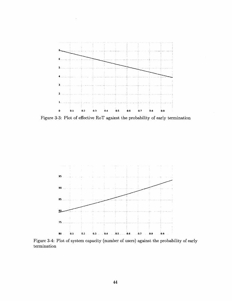
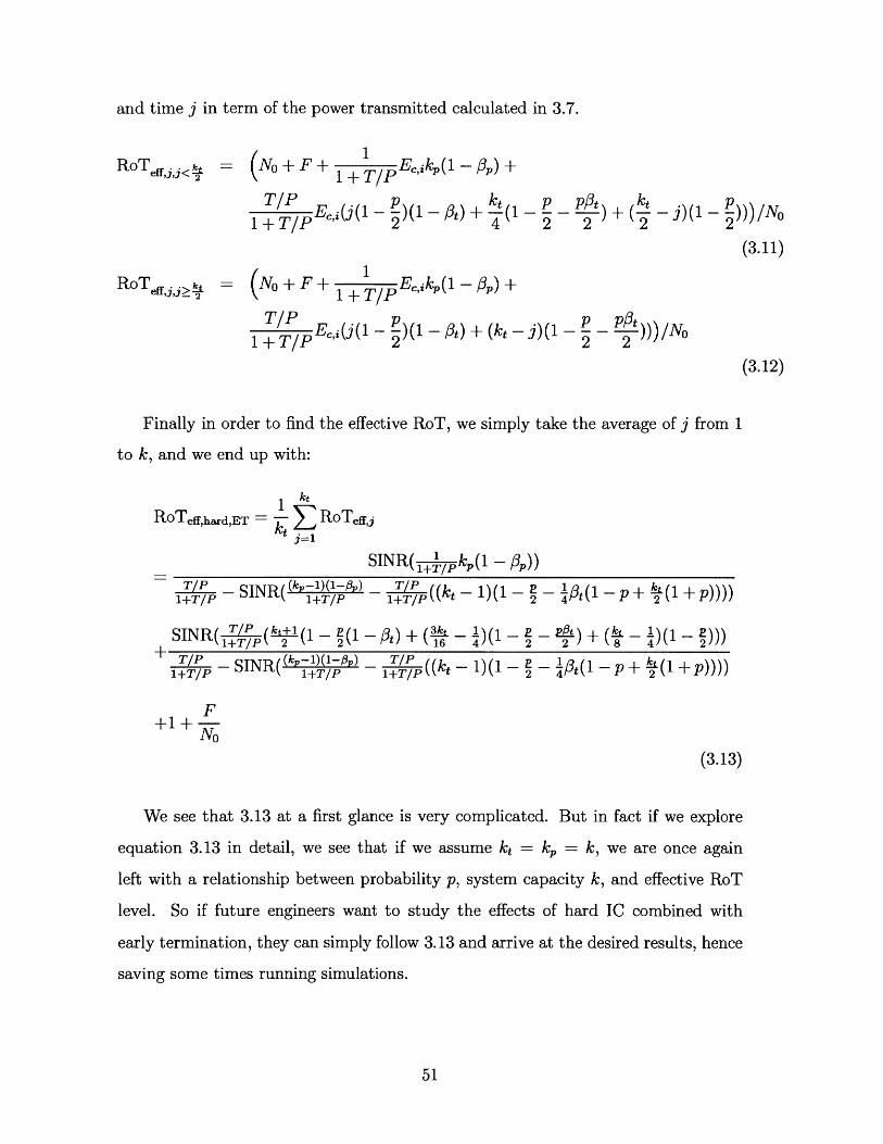
of early termination help us. So please refer to the following figures 3-3 and 3-4 where
we plot the relationship between effective RoT and p using data from table 2.4, and
also relationship between capacity of the system (number of users the system able
to support) and p with an effective RoT fixed at 6 dB. Also for the simplicity of
calculation, we assume k, = kt = k so we can extract all other parameters from the
simulation results from table 2.4. We observe that the relationship between both ca-
pacity and effective RoT with the probability of early termination tends to be linear.
3.3 Hard IC with early termination
3.3.1 Derivation
In this section we will add hard interference cancellation with early termination.
What we are trying to do here is that we would apply interference cancellation to
traffic channel signals whenever we have successfully decoded the received signal. This
6
3
2
1
0 01 02 03 04 0.5 0-6 07 0-8 09
Figure 3-3: Plot of effective RoT against the probability of early termination
95
00 01 0.2 0.3 0 0.5 06 07 08 09
Figure 3-4: Plot of system capacity (number of users) against the probability of earlytermination

means that if early termination is successful, we will apply traffic channel interference
cancellation to the first 15 slots of the received TTI, and if early termination does not
happen, we will not apply interference cancellation until the end of a TTI. In other
word, instead of before where we apply interference cancellation only at the end of a
TTI, we will try to early decode and apply interference cancellation at the half point
of a TTI. This implies that we would read each users' transmitted date 15 slots at a
time instead of 30 slots. We see that it can be rather difficult to calculate E, and
effective RoT, this is because the dependence between interference cancellation and
early termination.
In order to calculate E,, we again will need to argue that each user will transmit
at the same power. We will see this from user 1 and user kt's view again. In both
case we see that they see an equal amount of interference.
We see that when we're considering interference contribution from user j, there
are two cases, L > j > 2, and kt > j > k. For the sake of argument, we define kt
to be a multiple of 2 so it is relatively easy to model the problem. We see that for a
user j such that A2t j 2, we see that it has - fraction of data from the previous
TTI that may have early termination applied. Also - of user will have a chance2 uejilhaeacne
of getting early terminated since for j < L, the first half of j's current TTI will end
before user 1, therefore the base station would attempt an early termination. And if
early termination does happen, interference cancellation will be applied. And if early
termination does not happen, then at last k*-(j-1) of user j, meaning the part of user
j that's in the current TTI, have a 1 - p chance of no early termination therefore
no interference cancellation applied. So for the first & users, the contribution from
traffic channel to user 1's interference is:
ktt2 1 kt kt - (j - 1)(34Ect, (( - p) kt (1 - #A) +P p2 (1 -#)+ (1 -p)( )) (34
j=2
Then we consider the second case, we see that in this case j > kt. So we see there
are i-- of user j's power will have interference cancellation applied regardless
early termination happens or not. Then we see that there are k' of power having a

I user 11 2 3 user 2
4 5 6 user
The TT we are observingfrom user 1's view
Key: The bold rectangles represent thecurrent TTI that we're trying to decodeeach numbered region is represented by thesmallest rectangle enclosing the number
Figure 3-5: Demonstration of early termination with interference cancellation fromuser l's perspective
chance of 1-p not been terminated therefore having interference cancellation applied
because it is from the previous TTI and that TTI ends before user 1. At last there
is a fraction of k*-(j-1) amount of power not having any chance of early termination
or interference cancellation because it is in the current TTI and by the time the
base station finish reading user 1, it has not hit the half point of the current TTI
therefore no chance of early termination nor interference cancellation. So we see that
the contribution from those users' power into interference is:
kt j - 1 k,)( + 1_ kt I kt - ( j - 1))Ect; (( kt 2 )(2t 1-pg( 3 kt (3.5)j= +1
To make things clear, let's consider the diagram 3-5. User 2 can follow into the
first case. We see region 1 has a chance of p not been sent and 1 - p having interfer-
ence cancellation applied to. region 2 has a chance p been early terminated therefore
having interference cancellation applied to. And if user 2 does not early terminate
then both region 2 and region 3 would be seen by user 1 at full power because by the

ususer 2
erZL1U2I1I3.1I I_! ] 5 1 6
userkt
user k's equivalent view
Key: The bold rectangles represent thecurrent TTI that we're trying to decodeeach numbered region is represented by thesmallest rectangle enclosing the number
Figure 3-6: Demonstration of early termination with interference cancellation fromuser k's perspective
end of user l's observation it has not done transmitting in the current TTI. Then user
kt can be an example in the second case. Region 4 will have interference cancellation
applied regardless of user kt successfully early terminated or not in the previous TTI.
Region 5 has a chance p not being transmitted, and if early termination does not
happen, then region 5 would have interference cancellation applied to. Then region
6 will be seen by user 1 at full power regardless early termination happens or not.
So if we denote 3.4 as A and 3.5 as B, and also applying pilot interference cancel-
lation, we see that:
Ect,i = SINR(F + Ec,,(1 - o,) + A + B + No) (3.6)lEAp
With E,, = Ecg Vi # j. Also we see that in order to solve A and B, we can
simply break the sum apart and what we end up is solving a few arithematic sequence,

and we arrive at a solution to Eci:
SINR - (No + F)TIP -SINR((kp- -) + +P - 1)(- ) - p(1 -p (+ + P))))
(3.7)
Now we see that taking the effective RoT is not trivial either because of the inter-
ference cancellation. Just like in the previous chapter when we dealt with interference
cancellation without early termination, we have to find the RoT we observe at each
point in time during a TTI length of time, and we have to take the time average of
that RoT we observe as the effective RoT of the system. In this case with early ter-
mination, we can break up the problem into three cases by the time we are observing
RoT and also the user we are observing that is contributing to the RoT. Once again
in this case we have to divide time interval in a TTI into kt slots, and let i denote
the user number and j denote the time interval we are in.
In the first case let's consider i < j, this means that by the time j, the base station
has already finished decoding i, so regardless of early termination happens or not, we
would have applied interference cancellation to the entire TTI. The only difference is
that if early termination happens, we would only received the first half of the TTI.
therefore the interference seen from user i is:
p c (1 - #t) + (1 - p) Ec,j (1 - #t) = (1 -)Ec,j (1 - Pt) (3.8)2 2
In the second case let's consider when j ± ; > i > j, in this case we see that the
first half of user i has finished decoding by time j, but not the entire user i's TTI.
Therefore if early termination happens, then we would see interference cancellation
applied to the first half of the TTI. If early termination does not happen, then because
we would have decoded the entire TTI yet by time j, therefore we would see the entire
TTI in full power, meaning we would not have observed interference cancellation at

time j. So each user i's expected contribution to the interference is:
1p( Ec, (1 - #t)) + (1 - p)Ec,j (3.9)
2C,
In the last case let's consider kt ; i > j + , in this case regardless early ter-
mination happens or not, we would not be able to see any interference cancellation,
because at time j, the base station has not even finished decoding the first half of
user i's transmitted TTI. Therefore the interference we see from user i is:
(310p(1 Ec,j) + (1 - p)Ec,i (3.10)
Again following diagram 3-7, 3-8, and 3-9 as a three user example, one should be
able to see the above three cases more clearly. We see in all three diagrams we set
j = 1,meaning that we are trying to calculate the RoT at the time where first slot
ends. We see in 3-7, it follows case 1, we see that the entire user's TTI has already
finished decoding regardless of early termination happening or not. So for region 1 it
will have hard IC applied to it and region 2 and 3 will have a probability p of zero
power and I -p of interference cancellation application. Similarly in 3-8, region 1 and
2 will have interference cancellation applied regardless if early termination happens
and full power transmission if early termination doesn't happen. while region 3 and
4 will have a probability p of not transmitting and 1 -p of transmitting at full power.
In 3-9, user 3 will only has a chance of early termination and even if early termination
happens, hard IC will not apply to region 1 or 2.
Now we see that we can actually shorten the above 3 cases into 2 cases depending
only on the time j. We see that if j < a, then we have to perform summation of2'
i for all the 3 cases above, but if j > k, then we see that the last case would not2'
happen therefore we only have to consider the two cases where i < j and j + > i >
j =- kt > i > j. So again if we perform some summation of arithmatic sequence, we
arrive at the following two equations representing relationship between effective RoT

1 1 2 3 I
_I ~slot 1 slot 2
Figure 3-7: Case 1 of effective RoT calculation
Figure 3-8: Case 2 of effective RoT calculation
I
12 3 14slot 1 slot 2
Figure 3-9: Case 3 of effective RoT calculation
user 1L
user 2
user 3slot 3
user 1
user2
user3
user 1L
user 2
user 3slot 3
and time j in term of the power transmitted calculated in 3.7.
RoT effjj<!i (No +F+ 1 Eck,(1 - #p) +( 1 I
T/P pk± p ppt k1 + T/P Ec,i(j(1 - E)(1 - -) + (1 -
(3.11)1
ROT= (No+F+1+T/P Ecik(l - ) +
T/P Ec,i(j( - E)(1 - #t) + (kt - j)(1 2 --
1 +T/P 2,(( 2
(3.12)
Finally in order to find the effective RoT, we simply take the average of j from 1
to k, and we end up with:
1 kt
RoTeff,hard,ET = L RoTefj
j=1
SINR(4 k,(1 - #))T/P - SNT((kvl)(-haP) - TIP
1+T P SIR(k1T~ - 7 1+TIP ((kt - 1)(1 - - lt (1 - p + (1 + p))))
SINR(TP (ktl (1 _ (1 - #) + (3 - )(1 - - pt) + ( - )(1 -)))
1+TP TISINR((kP-1) 1-0B) _ TP ((kt - 1)(1 - - 1t (1 -p +(1 +p))))1TP 1l+lAlTIP~ 1+T/P2 4 P+-- I+A
F+1+-
(3.13)
We see that 3.13 at a first glance is very complicated. But in fact if we explore
equation 3.13 in detail, we see that if we assume kt = k, = k, we are once again
left with a relationship between probability p, system capacity k, and effective RoT
level. So if future engineers want to study the effects of hard IC combined with
early termination, they can simply follow 3.13 and arrive at the desired results, hence
saving some times running simulations.

52

Chapter 4
Soft IC
In this chapter we will discuss soft interference cancellation. Soft interference can-
cellation implies that we will cancel received signals from our base station buffer
regardless whether we successfully decoded the signal or not. This chapter will be
divided into two parts, where each part considers a different method of soft interfer-
ence cancellation. For the first part, we will consider pre-decoding soft interference
cancellation. it means that the base station will apply interference cancellation to
the received signals by attempting to make an estimation on each symbol right after
demodulation and not depending on the results of turbo decoding.This implies that
the base station will try to make some estimation of our channels and signals that
may not be as accurate as the decoded signals and add back the estimated signals
into the channel trying to achieve an improvement in the system performance. We
will consider a post-decoding soft interference cancellation scheme in the second part
of the chapter. This means that our signal estimation will be made on the soft output
from our turbo decoder, but once again we will make estimations and cancellations
without CRC passed.
The purpose of this chapter is to provide system engineers information regarding
whether one should apply soft or hard interference into the system. At the end of
each section we will give the required level of cancellation efficiency the system must
achieve in order to have the same performance as that of hard IC. In section we will
also give the equation relating SINR, #, RoT and k in each section.

4.1 Problem Setup
From [1], we see that there are a few ways for the base station to re-construct signals
and add the negated signal estimation into the channel to reduce interference. In
the case of soft interference cancellation, we see that we can make symbol estimation
to construct our desired signals. We know that each TTI is made of thousands of
symbols transmitting in sequence, so we see that this method of symbol estimation
is not as accurate as that we are reconstructing during hard interference cancellation
because we do not have CRC passed, meaning that we do not have a double check
for our signals to know for sure that we have decoded our signals correctly. But
we see that there are benefits of applying symbol estimation and soft interference
cancellation. We see in this chapter that using soft interference cancellation one can
see the benefits of the cancellation immediately, meaning that one does not have
to wait until the end of a TTI to apply cancellation. So in this chapter we will
explore the difference between soft interference cancellation and hard interference
cancellation, and make some conclusions about what cancellation efficiencies soft
interference cancellation must achieve in order to have the same effects as that of
hard interference cancellation. In other words, we are trying to make an evaluation
of the trade off between cancellation efficiency and the delaying in seeing the benefits
of interference cancellation.
To give a detailed description on how exactly one makes the symbol estimation,
we will consider equation 1.1 again. We have
k
g= Ais~;ibi + o-n-o (4.1)i=1
Where in the above equation b is each bit we are trying to send from user i and
s is the signature (or the OVSF that bi multiply to in the spreading process of 1-3)
of b2. o-no is white noise with variance a' Base station will be able to extract b2 by
multiplying g by c- and consider c- the receiver vector for user i. Presumably we

want cis= 1 iffi = j. Then we have:
k;T-= - = ({sbj = A-bc(T;) + ZAj'ciTs)xj ±ni (4.2)
j=1 i
We see that Abi(;Ts;) is our desired information, and all the rest of the terms
can be treated as noise. Therefore our definition of SINR is:
|ci Si)|A?SINR = 0 (' T-I) 2 (4.3)0.2 + ( s A
j54i
From 4.2, we see that we can make an estimation of bi by take bi = sign(yi). And
assume our estimation of bi is reasonable, we see that if we subtract our estimated be
from the received signal y, we can reduce the interference. We will apply cancellation
as follows: first we make an estimation for each bi for i = 1, ... , k, and we will store
our estimations in memory. Then we will re-interpret each symbol bi by subtracting
all b, j j4 i from y. We define:
y= Aibisi + ( Aj(bj - bj)sj+ a-nro (4.4)
With y,', we obtained a received signal with less interference for user i, therefore
if we again make an estimation of bi by taking sign(cy'). We see our estimation of
bi now depends heavily on how well our estimation for each other bj is. Therefore we
have to define a symbol level cancellation efficiency where it calculates on expectation
how close our estimation is to the real signal, normalized to one:
Cancellation efficiency =# = 1 - E[ b| - bi12] (4.5)
We will not have explicit calculation of what # is in each scenarios presented in
this chapter. The goal of the chapter is to evaluate what # level one must achieve
in order for soft interference cancellation to have the same gain as hard interference

Figure 4-1: Pre-decoding Soft Interference Cancellation Demonstration
cancellation.
We will also discuss some different approach of soft interference cancellation. As
mentioned above, the first case is that we will try to consider each symbol by itself
and trying to apply cancellation to each symbol therefore each user will be able to see
the effects of cancellation at a symbol level. Then we will consider soft interference
cancellation in a bigger time interval. And in the second case we will also assume a
different #A because we will use output of turbo decoder, therefore we assume that we
can achieve a better #t. The process of We consider cancellation every half of a TTI,
meaning that we will make an estimation of the signals received every half of a TTI.
In this case we see that we will have more delays in seeing the benefits of interference
cancellation, but intuitively we will have a higher cancellation efficiency because we
have read many more data therefore we are able to have better estimation.

User 1User 2
ii' 1userktConsider eachsymbol
al
a2
ak
Making anestimation foreach symbol a2
Sk,
Figure 4-2: Symbol level cancellation
4.2 Symbol Level Cancellation
We will consider a basic symbol level cancellation. According to [5] and [6], we
simply take each symbol one at a time and subtract our estimated signal immediately
to our traffic channel. Consider figure below, We see that our cancellation scheme
now looks very similar to that of pilot channel interference cancellation because of
the non synchronicity arrival of different user's traffic channel data will not affect
our perception of interference for each user. We see that we will just apply the
cancellation to each symbol immediately after we made the estimation. Therefore
with pilot interference cancellation, our SINR relationships between user's power and
interference is:
(4.6)Ec,i = SINR(No + F + Ec,1 -Iso) + j Ec,,i(1 -,))jEAt lEA,

From symmetry, we see that each user will be transmitting at:
E~i T/P SINR - (No + F) (4.7)- SINR( T/P (k, - 1)(1 - #sft) - 1(P - -
We see that in order to calculate rise over thermal (RoT) we see that we can just
follow our procedure from the hard IC chapter. During each time frame, we see that
the perspective RoT seen by the base station will be reduced by a factor of 1 - 3soft.
So our effective RoT is:
SINR- (ke(1 - tsof) P - k, f)RoTefr,sort,symboi =-r TP (TP-+I +I
1+T/P SINR( (k, - 1)(1 - sft) - 1 /p (k, - 1)(1 -
F+1 + F(4.8)
No
Now reference to 2.25, we see that if we fix effective RoT to 6 dB, and express
the soft interference cancellation efficiency against the hard interference cancellation
efficiency, we have an approximation of #sot ~ z .hard This implies that if we can have
a symbol estimation accuracy of more than 0.46, we can achieve better results with
soft interference cancellation.
4.3 Soft IC every half of a TTI
In this section we will consider post decoding soft interference cancellation. Referring
to figure 4-3, we can treat our turbo decoder as blackbox and we assume that after
we read every half of a TTI (15 slots), the turbo decoder will give us an estimation
of the signals and we can subtract the estimation from our buffer with cancellation
efficiency #soft,15. The details on exactly how one can estimate and reconstruct based
on turbo decoder's soft output is presented in [1], but our interest in this section is
to study the relationship between soft,15 and effective RoT.
We will consider the interference seen by each user. From figure 3-5, we see that
in addition to what we have cancelled from 2.21, each user will see an additional
cancellation of - - jEt,j from all other users. For every user, there are - users22 2
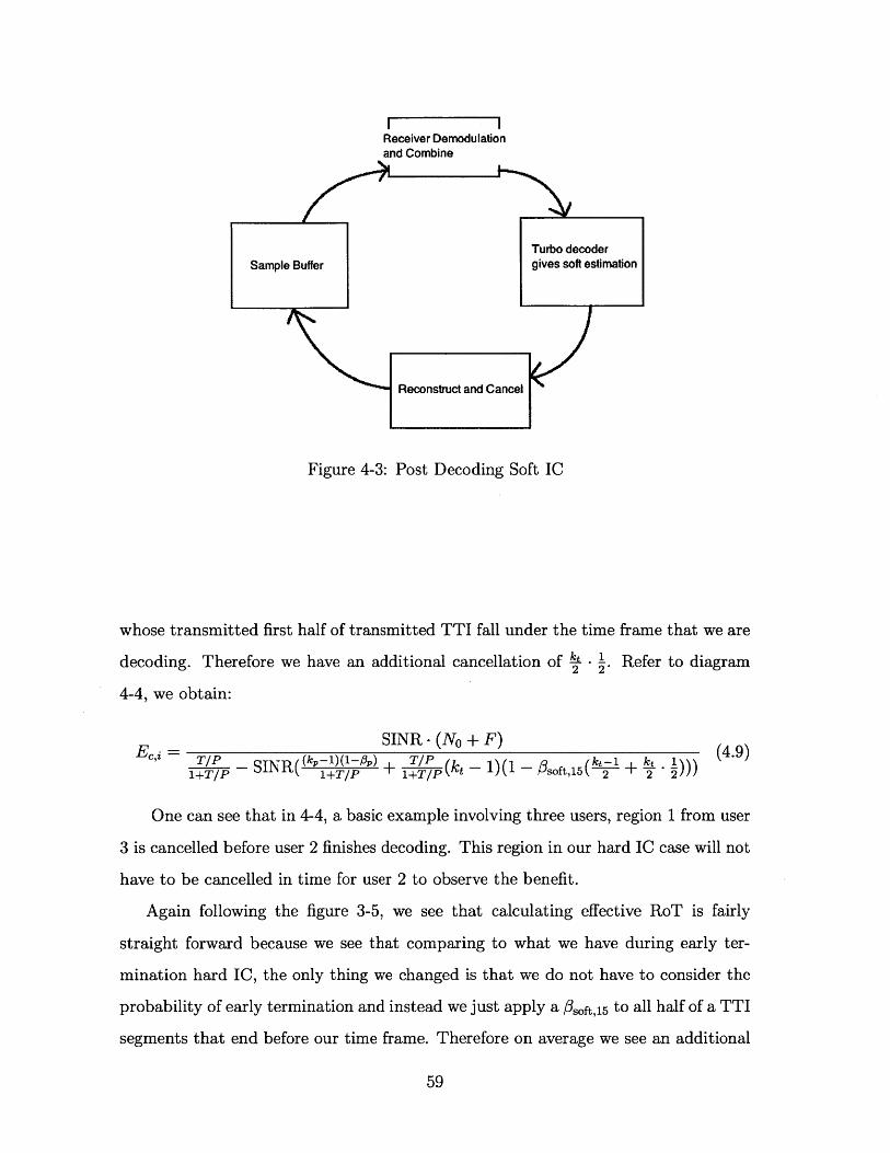
I IReceiver Demodulationand Combine
Figure 4-3: Post Decoding Soft IC
whose transmitted first half of transmitted TTI fall under the time frame that we are
decoding. Therefore we have an additional cancellation of k* - } Refer to diagram2 2
4-4, we obtain:
STSINR - (No + F)+E(g-ft5= _ (4.9)c /P -SINR( - ") + T/P (k - 1)(1 -k(t~ 2 2*1+T/P 1+T/P 1+T/P 2 2 2
One can see that in 4-4, a basic example involving three users, region 1 from user
3 is cancelled before user 2 finishes decoding. This region in our hard IC case will not
have to be cancelled in time for user 2 to observe the benefit.
Again following the figure 3-5, we see that calculating effective RoT is fairly
straight forward because we see that comparing to what we have during early ter-
mination hard IC, the only thing we changed is that we do not have to consider the
probability of early termination and instead we just apply a #soft,15 to all half of a TTI
segments that end before our time frame. Therefore on average we see an additional

user 1
user 2
user3
User 2's view
Region 1:Gray: Interference Cancellation seen by user 2Bold rectangle: Current TTIWe see that in hard IC whenone is trying to decode user 2at the end of the frame, it cannot see the benefits of cancelingregion 1, but using soft IC onecan observe it
Figure 4-4: Soft IC every 15 slots
k - of RoT is cancelled comparing to the hard IC case. So our effective RoT is:
-SINR(k, -7~ j+ (kt - (kt + Y)#soft,15) 1 )RoTeff,soa±,15 SP - SNR( (kp-1)(1-#son) + TPkt 1)(1 ( OsOft ~15k2 + -)1 +T/P 1+T/P 1+T/P ,5 2 2 2
F+1 + (4.10)
No
In this case if we take values from 2.4, we see that if we can achieve a #soft,15 of
0.64 (70.15 % of hard IC i) or more, we will achieve a better system capacity than
applying hard interference cancellation. We see that in this case we sacrificed some
cancellation efficiency requirement (a 20 % raise from the previous section) to enable
us to get some time delay in cancellation.
4.4 Results and Qualitative Analysis
From the above two sections we derived the perspective soft interference cancellation
efficiency the system has to achieve in order to out perform hard interference cancel-
lation. This gives insight to engineers when deciding which interference cancellation

algorithm to implement. In fact even in the case that soft interference cancellation
efficiency is lower than the threshold presented (46 % for symbol level and 64 % for
every half of a TTI), one may still want to consider soft cancellation because im-
plementing soft interference cancellation is simple. We see from the problem setup
section that in order to apply soft interference cancellation, one just need to demod-
ulate the received signal and make an estimation on each extracted symbol, where as
in hard interference cancellation we need to turbo decode and pass CRC in order to
apply cancellation.
Another issue where engineers have to make comparisons between the two IC al-
gorithms is memory allocation. We see that in the problem set up we would store
all of the estimated symbols into memory and subtract them from the buffer when
necessary. This may require a lot of memory comparing to hard IC because in hard
IC we simply reconstruct the TTI after CRC passed and we do not have to store our
reconstructed signals anywhere.

62

Chapter 5
Conclusion and possible future
work
As mentioned in the introduction, the thesis is helpful for engineers to improve the
existing WCDMA system. Throughout the thesis, we have shown the reliability of
the work comparing to existing simulations. Then we made comparisons between
performance of soft IC, hard IC, early termination and combinations between them.
We were able to see that soft IC requires a significant less cancellation efficiency to
out perform hard IC.
Even though the results from this thesis already give some intuition and theo-
retical back up for engineers to decide whether one should replace hard interference
cancellation with soft interference cancellation. There are still possible study one can
explore. First one can see that we only considered two soft interference cancellation
scenario. In fact in most current WCDMA system, one attempts to early terminate
every quarter of a TTI, this implies that we have three early termination probability,
namely p1,p2,p3 with p3 > P2 > pi. Each of the pi denote the chance of termination
at the end of that quarter of TTI. We can easily in the baseline scenario our power

transmitted will be in term of P1 + P2 + p3:
SINR - (No + F)
TP- SINR( 1/ (p-1+ TP (t -111+( P1) + (1 -P2) + (1 ~-P3)))1T/5 -+I +TP 1kY TP4
(5.1)
From the equation above, we can try to explore the effects of applying interfer-
ence cancellation to multiple early termination schemes. In fact we can also explore
the possible cancellation efficiency the system can achieve if we condition the type of
cancellation on the success of early termination. Meaning that we will apply hard IC
if we decode successfully and soft IC if we do not.
One other thing we can explore is early termination combined with soft inter-
ference cancellation. We have four variables in this case: effective RoT, number of
users, probability of early termination, and soft interference cancellation efficiency.
We can make a plot or a table relating all four variables. Then when engineers explore
the feasibility of soft interference cancellation, they can look up the corresponding
parameters to determine what to implement into the system.

Bibliography
[1] W. Zeng, S. Sambhwani, W. Zhang, and J. K. Wegrzyn. "Iterative Soft Interfer-
ence Cancellation for HSPA Uplink." VTC 2010-Fall, 2010 IEEE 72nd, page 1-5.
September 2010
[2] J. Hou, J. E. Smee, H. D. Pfister, and S. Tomasin. "Implementing Interference
Cancellation to Increase the EV-DO Rev A Reverse Link Capacity." IEEE Trans-
actions on Communication, February 2006
[3] Danlu Zhang, Sharad Sambhwani, and Bibhu Mohanty. "HSUPA Scheduling al-
gorithms Utilizing RoT Measurements and Interference Cancellations." in Proc.
ICC, 2008, pp.5033-5037
[4] Yeliz tokgoz, Mingxi Fan, and John E. Smee. "On the Reverse Link Performance
of the cdma2000 1xEV-DO Revision A system with Antenna Array Receivers."
IEEE Globecome 2005, pp. 3373-3377
[5] S. Verdu, Multiuser Detection. New York, USA: Cambridge University Press,
1998.
[6] Divsalar, M. K. Simon, and D. Raphaeli, "Improved parallel interference cancel-
lation for CDMA," IEEE Transactions on Communications, vol. 46, no. 2, pp.
258-268, Feb. 1998
[7] A. Viterbi, "Very low rate convolutional codes for maximum theoretical perfor-
mance of spread-sprectrum multiple-access channels," IEEE Journal on Selected
Areas in Communications, vol. 8, no. 4, pp. 641-649, May 1990

[8] X. Wang and H. V. Poor, "Iterative (turbo) soft interference cancellation and
decoding for coded CDMA, " IEEE Transactions on Communications, vol. 47, no.
7, pp. 1046-1061, July 1999
[9] S. Sambhwani, W. Zhang, and W. Zeng, "Uplink interference cancellation in
HSPA: Principles and practice, " 2008, Qualcomm White Paper