a study on an automatic system for analyzing the … · a study on an automatic system for...
TRANSCRIPT
A Study on an Automatic System for Analyzing the
Facial Beauty of Young Women
Neha Sultan
A Thesis
in
The Department
of
Computer Science and Software Engineering
Presented in Partial Fulfillment of the Requirements
For the Degree of Master of Computer Science at
Concordia University
Montreal, Quebec, Canada
January 2014
© 2014 Neha Sultan

CONCORDIA UNIVERSITY
School of Graduate Studies
This is to certify that the thesis prepared
By: Neha Sultan
Entitled: A Study on an Automatic System for Analyzing the
Facial Beauty of Young Women
and submitted in partial fulfillment of the requirements for the degree of
MASTER OF COMPUTER SCIENCE
complies with the regulations of the University and meets the accepted standards with
respect to originality and quality.
Signed by the final Examining Committee:
________________________________ Chair
Dr. Jayakumar Rajagopalan
________________________________ Examiner
Dr. Tonis Kasvand
________________________________ Examiner
Dr. Yuhong Yan
________________________________ Thesis Supervisor
Dr. Ching Y. Suen
Approved by ___________________________________________________
Chair of Department or Graduate Program Director
___________________________________________________
Dr. Christopher Trueman, Dean,
Faculty of Engineering and Computer Science
Date ____________________________________________________

ACKNOWLEDGEMENTS
My supervisor, Dr. Ching Y. Suen has provided me with constant guidance and invaluable
feedback. I would also like to extend my gratitude to the Centre for Pattern Recognition
and Machine Intelligence (CENPARMI) at Concordia University for providing the
perfect environment for enabling innovation and excellence in research. I also thank the
Natural Sciences and Engineering Research Council for the support associated with this
research. In addition, the Faculty of Engineering and Computer Science at Concordia
University has been a great source of invaluable knowledge and support for which I am
grateful.
I would like to thank my family for always being there for me and for all their support.

DEDICATION
This thesis is dedicated to my parents, who encourage and support me constantly and due
to their guidance I have been able to achieve my goals.
iii
ABSTRACT
A Study on an Automatic System for Analyzing the Facial Beauty of Young Women
Neha Sultan
Beauty is one of the foremost ideas that define human personality. However, only
recently has the concept of beauty been scientifically analyzed. This has mostly been due
to extensive research done in the area of face recognition and image processing on
identification and classification of human features as contributing to facial beauty.
Current research aims at precisely and conclusively understanding how humans classify a
given individual's face as beautiful. Due to the lack of published theoretical standards and
ground truths for human facial beauty, this is often an ambiguous process. Current
methods of analysis and classification of human facial beauty rely mainly on the
geometric aspects of human facial beauty. The classifiers used in current research include
the k-nearest neighbor algorithm, ridge regression, and basic principal component
analysis.
In this research, various approaches related to the comprehension and analysis of human
beauty are presented and the use of these theories is outlined. Each set of theories is
translated into a feature model that is tested for classification. Selecting the best set of
features that result in the most accurate model for the representation of the human face is
a key challenge. This research introduces the combined use of three main groups of
features for classification of female facial beauty, to be used with classification through
support vector machines. The classifier utilized is Support Vector Machine (SVM) and
the accuracy obtained through this classifier is 86%. Current research in the field has

iv
produced algorithms with percentages of accuracy that are in the range of 75-85%. The
approach used is one of analysis of the central tenets of beauty, the successive application
of image processing techniques, and finally the usage of relevant machine learning
methods to build an effective system for the automatic assessment of facial beauty. The
ground truths used for verifying results are derived from ratings extracted from surveys
conducted.
The proposed methodology involves a novel algorithm for the representation of facial
beauty, which combines the use of geometric, textural, and shape based features for the
analysis of facial beauty. This algorithm initially develops an overall landmark model of
the entire human face. A significant advantage of this methodology is the accurate model
of the human face which synthesizes the geometric, textural and shape-related aspects of
the face. The landmark model is then used for extracting critical characteristics which are
then used in a feature vector for training using machine learning. The features extracted
help to represent facial characteristics in three major areas. Geometric features help to
represent the symmetrical properties and ratio-based properties of landmarks on the face.
Textural features extracted help capture information related to skin texture and
composition. Finally, face shape and outline features help to categorize the overall shape
of a given face, which helps to represent the given female face shape and outline for
further analysis of any deviations from the basic face shapes. These features are then used
in a classifier to appropriately categorize each image. The database used for the source of
images contains images of female subjects from a variety of backgrounds and levels of
attractiveness.
v
TABLE OF CONTENTS
LIST OF FIGURES .................................................................................................................. XI
LIST OF TABLES .......................................................................................................... xiv
CHAPTER 1 INTRODUCTION ............................................................................................ 1
1.1 Related Fields of Research ......................................................................................... 2
1.1.1 Facial Expressions and Emotions .......................................................................... 3
1.1.2 Composite Faces .................................................................................................... 5
1.1.3 Gender Classification ............................................................................................. 8
1.1.4 Facial Beauty Analysis ......................................................................................... 10
1.2 Problem Description ................................................................................................. 13
1.3 Main Contributions .................................................................................................. 14
1.4 Applications of Automatic Beauty Analysis ............................................................ 16
CHAPTER 2 STANDARDS AND THEORIES ASSOCIATED
WITH FACIAL BEAUTY ............................................................................ 17
2.1 Beauty Throughout the Ages .................................................................................... 17
2.1.1 Pythagoras's Contributions .................................................................................. 18
2.1.2 The Golden Ratio ................................................................................................. 19
2.1.3 Plato ..................................................................................................................... 21
2.1.4 Aristotle ................................................................................................................ 22
2.2 Modern Philosophy ................................................................................................... 22
2.3 Evolution and Beauty ............................................................................................... 23
2.4 Objectivity of Facial Beauty ..................................................................................... 24
vi
2.5 Theories Related to Facial Beauty ........................................................................... 26
2.5.1 Averageness .......................................................................................................... 26
2.5.2 Symmetry ............................................................................................................. 27
2.5.3 Skin Texture ......................................................................................................... 27
2.5.4 Geometric Facial Features ................................................................................... 28
2.5.5 Golden Ratio ........................................................................................................ 28
2.5.6 Facial Thirds ........................................................................................................ 29
CHAPTER 3 DATA ANALYSIS AND COLLECTION .................................................. 30
3.1 Databases Utilized in this Research ......................................................................... 33
3.1.1 AR Face Database ................................................................................................ 34
3.1.2 Psychological Image Collection at Stirling ......................................................... 36
3.1.2.1 Stirling Faces Database ................................................................................. 36
3.1.2.2 Nottingham Faces Database .......................................................................... 37
3.1.2.3 Utrecht Database ........................................................................................... 38
3.1.2.4 FEI Face Database ........................................................................................ 39
3.1.2.5 Indian Face Database Beauty Queens ........................................................... 40
3.1.2.6 Images of Beauty Pageant Contestants ......................................................... 40
3.2 Survey Methodology ................................................................................................. 41
3.2.1 Participants for the Survey ................................................................................... 41
3.2.2 Data Set ................................................................................................................ 42
3.2.3 Procedure and Ratings Collection ........................................................................ 43
3.2.4 Ratings Analysis................................................................................................... 45

vii
CHAPTER 4 DEVELOPMENT OF REPRESENTATIONAL MODEL
FOR ASSESSING FACIAL BEAUTY....................................................... 47
4.1 Active Shape Models ................................................................................................. 49
4.2 Shapes......................................................................................................................... 49
4.3 Landmarks................................................................................................................. 51
4.4 Shape Alignment ....................................................................................................... 51
4.5 Profile Model ............................................................................................................. 53
4.6 Shape Model .............................................................................................................. 55
4.7 ASM Image Search ................................................................................................... 56
4.8 Fitting Generated Model to Given Points ............................................................... 57
4.9 Processing Results ..................................................................................................... 58
CHAPTER 5 FORMULATION OF ALGORITHM FOR BEAUTY ANALYSIS .... 60
5.1 Facial Representation ............................................................................................... 61
5.2 Geometric Features ................................................................................................... 63
5.2.1 Ratios Pertaining to Major Facial Regions .......................................................... 66
5.2.1.1 Eye Features .................................................................................................. 66
5.2.1.2 Nose Features ................................................................................................ 68
5.2.1.3 Mouth Area Features ..................................................................................... 71
5.2.2 Ratios Pertaining to Facial Beauty Theories ........................................................ 73
5.2.2.1 Features based on Facial Thirds Method ...................................................... 77
5.3 Texture Analysis ........................................................................................................ 79
5.4 Face Shape Analysis .................................................................................................. 88
5.4.1 Edge Gradient and Face Contour ......................................................................... 91
viii
CHAPTER 6 EXPERIMENTAL RESULTS ..................................................................... 96
6.1 Feature Classification ............................................................................................... 98
6.1.1 Support Vector Machines ..................................................................................... 98
6.1.1.1 Nonlinear Classification.............................................................................. 101
6.1.1.2 Multiclass Approaches ................................................................................ 103
6.2 Correlations in Results ........................................................................................... 105
6.3 Training Database ................................................................................................... 107
6.4 Testing Database...................................................................................................... 109
6.5 Values Utilized .......................................................................................................... 111
CHAPTER 7 ILLUSTRATIVE EXAMPLES ................................................................ 113
7.1 Attractiveness Level 1 .............................................................................................. 114
7.1.1 Geometric Features ............................................................................................ 114
7.1.2 Textural Features ................................................................................................ 115
7.1.3 Facial Shape Features ........................................................................................ 116
7.2 Attractiveness Level 2 .............................................................................................. 117
7.2.1 Geometric Features ............................................................................................ 117
7.2.2 Textural Features ................................................................................................ 118
7.2.3 Facial Shape Features ........................................................................................ 119
7.3 Attractiveness Level 3 .............................................................................................. 119
7.3.1 Geometric Features ............................................................................................ 119
7.3.2 Textural Features ................................................................................................ 120
7.3.3 Facial Shape Features ........................................................................................ 121

ix
7.4 Attractiveness Level 4 ............................................................................................. 122
7.4.1 Geometric Features ............................................................................................ 122
7.4.2 Textural Features ................................................................................................ 123
7.4.3 Facial Shape Features ........................................................................................ 124
7.5 Attractiveness Level 5 ............................................................................................. 125
7.5.1 Geometric Features ............................................................................................ 125
7.5.2 Textural Features ................................................................................................ 126
7.5.3 Facial Shape Features ........................................................................................ 127
7.6 Miss World 2010 ...................................................................................................... 128
7.6.1 Geometric Features ............................................................................................ 128
7.6.2 Textural Features ................................................................................................ 129
7.6.3 Facial Shape Features ........................................................................................ 130
7.7 Miss Universe 2010 ................................................................................................. 131
7.7.1 Geometric Features ............................................................................................ 131
7.7.2 Textural Features ................................................................................................ 132
7.7.3 Facial Shape Features ........................................................................................ 133
7.8 Elizabeth Taylor ...................................................................................................... 133
7.8.1 Geometric Features ............................................................................................ 134
7.7.2 Textural Features ................................................................................................ 135
7.7.3 Facial Shape Features ........................................................................................ 136
7.9 Marilyn Monroe ...................................................................................................... 137
7.9.1 Geometric Features ............................................................................................ 137

x
7.9.2 Textural Features ................................................................................................ 138
7.9.3 Facial Shape Features ........................................................................................ 139
CHAPTER 8 CONCLUSIONS AND FUTURE WORK ............................................. 140
8.1 Conclusions .............................................................................................................. 140
8.2 Future Work ............................................................................................................ 141
REFERENCES ...................................................................................................................... 143

xi
LIST OF FIGURES
Figure 1: Illustration of the composite face illusion. Here the top halves of the images are
all identical, and they are paired with different bottom halves of images. This
gives the illusion that the top halves of the images are also different. ............... 7
Figure 2: Composite faces representing various nationalities [9] ....................................... 8
Figure 3: Images with no enhanced symmetry (left) and an image with enhanced
symmetry (right) ................................................................................................11
Figure 4: Distribution of respondents preferring symmetry ............................................. 12
Figure 5: Representation of Golden Ratio on a Human Face ........................................... 21
Figure 6: Sample Images from AR Face Database ........................................................... 36
Figure 7: Original images from Stirling database [27] .................................................... 37
Figure 8: Original images from Nottingham database [27] .............................................. 38
Figure 9: Original images from Nottingham database [27] .............................................. 39
Figure 10: An excerpt from the survey ............................................................................. 44
Figure 11: A shape represented by a set of points connected by edges, a set of x and y
coordinates and as a vector representation. ...................................................... 50
Figure 12: Example of construction of profile vector ....................................................... 54
Figure 13: The mean face shape model (black line) and the variations on the model (gray
lines) ................................................................................................................. 56
Figure 14: Final fit of model to a sample image ............................................................... 58
Figure 15: Facial landmarks outlined ............................................................................... 65
Figure 16: Detailed diagram of eye [56] ........................................................................... 67

xii
Figure 17: Various measurements taken of the nose [57] ................................................. 69
Figure 18: Major features of the nose ............................................................................... 70
Figure 19: Landmarks of the mouth.................................................................................. 72
Figure 20: Representation of measurements from Table 9 ............................................... 74
Figure 21: Facial Thirds: The three regions on a face ...................................................... 78
Figure 22: Various textures represented ............................................................................ 80
Figure 23: Images corresponding to the various texture representations and
attractiveness levels: top left: attractiveness rating of 5, top center:
attractiveness rating of 4, top right: attractiveness rating of 3,
bottom left:attractiveness rating of 2, bottom left:attractiveness rating of 1 .... 88
Figure 24: Various face shapes illustrated ........................................................................ 90
Figure 25: Various steps of dividing the image into subregions ....................................... 92
Figure 26: Face shape outline ........................................................................................... 93
Figure 27: Masks for the various orientations: (from left) vertical, horizontal,
diagonal1, diagonal2, non-directional) ............................................................. 95
Figure 28: Block Diagram of Beauty Analysis System .................................................... 97
Figure 29: Illustration of possible hyperplanes in a SVM .............................................. 100
Figure 30: Construction of two main hyperplanes .......................................................... 101
Figure 31: Illustration of mapping to higher dimension in SVM classification ............. 102
Figure 32: Initial data for illustration of nonlinear classification ................................... 102
Figure 33: Classified data for nonlinear classification ................................................... 103
Figure 34: Illustration of one-versus-one approach for multiclass SVM ....................... 105
Figure 35: Number of Images in Training Database Corresponding to each Rating ...... 109
xiii
Figure 36: Number of Images in Testing Database Corresponding to each Rating ......... 111
Figure 37: Samples of incorrectly classified images .......................................................112
Figure 38: Image with attractiveness rating of 1 .............................................................114
Figure 39: Image with attractiveness rating of 2 .............................................................117
Figure 40: Sample image with attractiveness rating of 3 .................................................119
Figure 41: Sample image with attractiveness rating of 4 ................................................ 122
Figure 42: Sample image with attractiveness rating of 5 ................................................ 125
Figure 43: Image of Miss World 2010 ............................................................................ 128
Figure 44: Image of Miss Universe 2010 ....................................................................... 131
Figure 45: Image of Elizabeth Taylor ............................................................................. 133
Figure 46: Image of Marilyn Monroe ............................................................................. 137

xiv
LIST OF TABLES
Table 1: Descriptions of Main Facial Expressions ............................................................. 5
Table 2: Data related to the Survey Participants ............................................................... 42
Table 3: Percentage of Images at each Level of Attractiveness ........................................ 45
Table 4: Sizes tested with their corresponding results ...................................................... 64
Table 5: Features related to the eye ................................................................................... 68
Table 6: Ratios related to the nose .................................................................................... 71
Table 7: Ratios related to the mouth ................................................................................. 73
Table 8: Measurements taken for Geometric Representation of Face .............................. 75
Table 9: List of Ratios Associated with the Golden Ratio ................................................ 76
Table 10: List of Ratios Associated with the Facial Thirds theory ................................... 78
Table 11: Textural features obtained ................................................................................. 86
Table 12: Results Achieved for each SVM Kernel Function .......................................... 105
Table 13: Correlations of Feature Measurements with Attractiveness Ratings .............. 106
Table 14: Values of sample geometric measurements .....................................................115
Table 15: Values of sample textural features ...................................................................116
Table 16: Values of sample geometric measurements .....................................................118
Table 17: Values of sample textural features ...................................................................119
Table 18: Values of sample geometric measurements .................................................... 120
Table 19: Values of sample textural features .................................................................. 121
Table 20: Values of sample geometric measurements .................................................... 123
Table 21: Values of sample textural features .................................................................. 124

xv
Table 22: Values of sample geometric measurements .................................................... 126
Table 23: Values of sample textural features .................................................................. 127
Table 24: Values of sample geometric measurements .................................................... 129
Table 25: Values of sample textural features .................................................................. 130
Table 26: Values of sample geometric measurements .................................................... 132
Table 27: Values of sample textural features .................................................................. 133
Table 28: Values of sample geometric measurements .................................................... 135
Table 29: Values of sample textural features .................................................................. 136
Table 30: Values of sample geometric measurements .................................................... 138
Table 31: Values of sample textural features .................................................................. 139

1
Chapter 1 Introduction
“Beauty is the shadow of God on the universe”, said Gabriela Mistral, who lived on to
become the first Latin American to win the Nobel Prize in Literature. People have often,
though stereotypically, believed that what is good is beautiful. Due to the inherent
tendencies of human beings, objects and creatures with features and appearances that are
appealing to the eyes have traditionally been associated with positive responses and
attributes. These and many more observations regarding the concept of beauty continue to
intrigue and mystify humans. The aesthetic aspects of most animate and inanimate
objects have been known to capture the undivided attention of great thinkers and
scientists throughout history. It is indisputably human nature to ponder and marvel at the
intricacies and beauty of people and objects surrounding us. Even more characteristic of
humans is the tendency to focus on associated facial features and their indisputable
connection with beauty.
The human face conveys extensive amounts of information; in essence, it speaks volumes
about the individual it is associated with. Millions of dollars are spend on facial
beautification and cosmetics; it has been shown that the amount of money spent on
beauty related products in the US is more than the amount spent on education and social
services [1]. Research has even conclusively shown that attractive faces activate centers
of the brain that are associated with reward [2]. Studies have demonstrated that attractive
people get preferential treatment and thus have greater tendencies towards achieving
success. The socio-economic impact of facial beauty therefore helps stress the greater
need for understanding of this basic concept. Significant amounts of research have been

2
conducted in the area of face analysis and recognition, a considerable portion of this
research being in the area of facial beauty.
Science strives to explain the various phenomena of nature and hence it concurs naturally
that the concept of beauty be approached and deciphered through the scientific method.
This thesis attempts to describe and analyze extensively the concept of beauty from a
technical perspective. It concentrates on building an automatic system for the
measurement of female facial beauty. The approach used is one of analysis of the central
tenets of beauty, the successive application image processing techniques, and finally the
usage of relevant machine learning methods to build an effective system for the automatic
assessment of facial beauty.
The ground truths used for verifying results are derived from ratings extracted from
surveys conducted. Several key aspects and features that have been extensively shown to
be associated with beauty will be discussed and then eventually utilized as features and
main components. These features will then be used in a classifier to appropriately
categorize each image.
1.1 Related Fields of Research
Research in the area of facial image processing has contributed to numerous successful
studies. The human face itself has the potential to divulge great amounts of information
that could prove to be of great use to researchers. The most commonly studied area is that
of facial identity analysis. Additional areas include composite faces, human gender
determination, age determination, and facial expression and emotional analysis. We will
proceed to take a closer look at these related fields.

3
1.1.1 Facial Expressions and Emotions
Human facial expressions serve as an important component of communication between
individuals. They are essentially based on movements of muscles beneath the skin of the
face. Several studies in the area of machine learning have concluded in the creation of
computational models of facial expressions. These models are of great use to scientists as
facial expressions are of great importance in the fields of cognitive science, psychology,
and neuroscience. Models of human emotion are also of great importance in the areas of
artificial intelligence and human computer interaction systems.
Facial behaviors and expressions have numerous uses, which help aid in the daily
communication aspects of individuals. Some primary aspects include:
- People often use expressions to depict what they are conveying, such as raised
eyebrows for high pitches and lowered eyebrows for low pitches.
- Expressions are also used to control the flow of a conversation, for example
people may gesture to let others know that they have finished talking.
- Human expressions often serve as signals of mental processes occurring, such as
someone furrowing their brow when concentrating on a matter.
People also use expressions to consciously communicate their emotional states to other
individuals.
There are two main models for representing human facial expressions. The categorical
model assumes that there is a finite set of universal prevalent human expressions. These
expressions can be divided into six main classes, which include joy, surprise, anger,
4
sadness, disgust, and fear [4]. This model is disputable because it assumes that facial
expressions are universally innate, rather than dependent on culture. The continuous
model, on the other hand, simply models each emotion as a feature vector, which each
vector containing the various characteristics of each emotion.
By the categorical model, there are six main universal classified facial expressions which
include joy, surprise, anger, sadness, disgust, and fear. The Facial Action Coding System
helps to categorize facial expressions based on how they appear on an individual's face
and which muscle systems are involved. This also allows any machine to systematically
represent any facial expression in terms of constituent units called Action Units. Action
Units are basically individual groups of muscles and their corresponding actions. There
are approximately a hundred action units currently.
The main categories of Action Units are [5]:
- Main Action Unit Codes: these consist of basic facial muscle groups, such as
“cheek raiser”, “brow lower”, etc
- Head Movement Codes: these describe the position of the head, such as “head
turn left”, “head tilt right”, etc
- Eye Movement Codes: these describe where the eye is looking, such as “eyes turn
right”, “eyes looking at another person”, etc
- Visibility Codes: these help to describe which parts of the face are not visible,
such “brows and forehead not visible”, “lower face not visible”, etc
In order to classify facial expressions correctly, each facial expression is mapped to

5
several contributing action units and subsequently the facial images are analyzed for the
presence of such facial action units.
The Automatic Face Analysis system was developed by Tian et al for the analysis of
facial expressions based on the Facial Action Coding System. This system was trained
and developed to recognize and analyze facial expressions based on two main features,
which included permanent facial features and transient facial features. Table 1 illustrates
the various action units and characteristics associated with each facial expression.
Facial Expression
Number of
Action Units Description
Anger Four Mouth and lips tightened, lowered and furrowed
eyebrows, head facing straight ahead
Disgust Three Mouth open, upper lip raised, lower lip turned
down, cheeks raised, protruding lips
Fear Six Mouth open slightly, eyebrows raised,
perspiration, eyes wide open
Happiness Two Eyes wide open, mouth corners raised and
lowered, mouth pulled back at the corners, skin
under eyes has wrinkles
Sadness Three Mouth corners depressed and lowered, inner
portion of eyebrows raised
Surprise Four Arched eyebrows, eyes opened widely to expose
more white portion of eye, lips protruded, jaw
slightly dropped
Table 1: Descriptions of Main Facial Expressions
1.1.2 Composite Faces
Sir Francis Galton has long been known famously as one of the pioneers in the areas of
composite imaging, a lot of what is known about his methodology comes from his
6
extensive documentation called “Composite Portraits”, which was published in London
in 1878. The process essentially involved superimposing multiple exposures of various
individuals' faces on a single photographic plate. An inherently observant scientist, Sir
Galton, also hypothesized that these composite portraits would be more attractive than
the individuals used to create them. This has been known to be the basis of research in the
1900s on the influence of “averageness” on facial attractiveness[6]. Going further, Sir
Galton further proposed that these composite faces could also represent various human
ideals, concepts, and even various categories and characteristics of people. Concluding
from this, he began modeling composite faces that would represent features that were
commonly found in various types of humans, such as murderers, doctors, etc.
Significant changes have been made in this field, with major improvements in terms of
speed, accessibility and automation. Research has been done in automatic extraction and
blending of human faces into media content.
Another aspect of composite faces is one in which the picture is made up of two halves,
one half from one person and the other from another person, thus coming up with a new
image. Considerable studies have been done on the effects of these images. The human
brain can oftentimes effortlessly distinguish a face from the various other image patterns
available. Moreover, it does not require much effort to distinguish one face form another
as well. However, in the case of composite faces made up of two different humans, the
brain often faces an optical illusion [8].
When the same top half of a facial image is paired with various different bottom halves of
a facial image, the observer is often led to believe that the identical top halves might be

7
non-identical. This illusion, known as the composite face illusion, still occurs when the
viewer consciously knows that the top halves are in fact identical.
Figure 1: Illustration of the composite face illusion. Here the top halves of the images are
all identical, and they are paired with different bottom halves of images. This gives the
illusion that the top halves of the images are also different.
Composite faces have also been used to theoretically model “average” faces for women
of different nationalities and ethnicities. It has often been observed that these composite
faces are more attractive than the faces used to produce them. This has been hypothesized
to be due to the fact that in the process of calculating the composite images, any
irregularities and asymmetries present in the component faces become neutralized. The
skin on the resulting composite face looks very young and smooth, because any facial
marks such as pimples and wrinkles also disappear during the blending process.
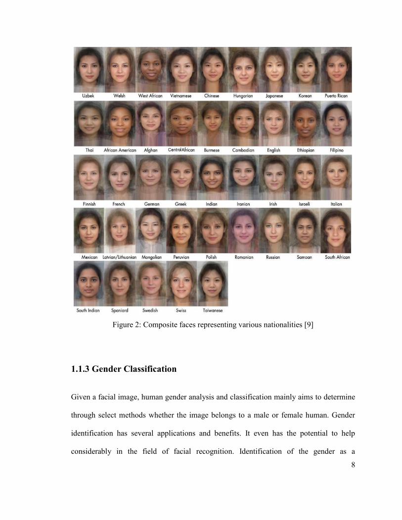
8
Figure 2: Composite faces representing various nationalities [9]
1.1.3 Gender Classification
Given a facial image, human gender analysis and classification mainly aims to determine
through select methods whether the image belongs to a male or female human. Gender
identification has several applications and benefits. It even has the potential to help
considerably in the field of facial recognition. Identification of the gender as a

9
preprocessing step for facial identification would technically make the process twice as
fast as it would initially classify the image set into two halves, one for the female
participants and one for the male. Gender classification is often important for the
development of human computer interaction systems that are able to evolve and
customize the experience of the user according to gender.
Currently many retail operations and are attempting to customize their general customer
experience by identifying the specific gender of the people passing by their outlets. This
eventually helps to target advertisement towards the specific related gender and in turn
increases revenue for the outlets. Several more important uses for gender identification
and analysis are as below:
- demographic data collection
- human computer monitoring
- robotics applications
- psychotherapy applications
- surveillance and security
- biometrics
Two main approaches to the problem of gender classification include feature based and
appearance based models [10]. In the feature based model, various features are extracted
from the image and the overall gender detection process is based on the analysis of those
features. Some examples of features commonly used include features extracted from the
geometry of the face, edge information, and even skin color information. The appearance
based model, on the other hand, basically aims to input the entire image as the basis of
analysis rather individual features of the image.
10
Several novel methods have been developed over the years in the area of gender
classification. Baluja and Rowley [11] used the Adaboost classifier, which helped them
achieve over ninety-three percent classification. This was higher than the accuracy that
they received with support vector machines, for which the input used pixels. The
Adaboost classifier also had considerable increases in speed, achieving fifty times faster
classifications than support vector machines.
1.1.4 Facial Beauty Analysis
Considerable research has been conducted in the areas of image processing and machine
learning. A certain portion of that has focused on aspects related to the human face. A
very integral aspect of the human face is its own characteristic natural beauty; beauty that
has inspired, motivated, and generated a considerable extent of debate and discussion.
The idea of quantifying beauty has been approached and extensively studied throughout
the ages. Therefore, various methodologies and theories have been proposed by several
leading scientists in the disciplines of image processing and machine learning. The
approach has varied greatly, with some focusing on aspects of measuring beauty through
human raters, some preferring to quantify beauty through regression techniques, while
others assessed the effects of certain factors on the perception of beauty. This section
presents the various scientific approaches to the analysis of human facial beauty.
Perett et al [23] examined the role of symmetry in the perception of beauty for a given
face. Several experiments were conducted to help determine the role and contribution of
symmetry. All experiments involved presenting a group of raters with a set of images to
rate according to their preferences. The first experiment involved making three
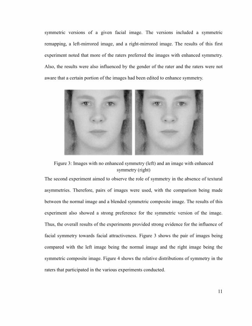
11
symmetric versions of a given facial image. The versions included a symmetric
remapping, a left-mirrored image, and a right-mirrored image. The results of this first
experiment noted that more of the raters preferred the images with enhanced symmetry.
Also, the results were also influenced by the gender of the rater and the raters were not
aware that a certain portion of the images had been edited to enhance symmetry.
Figure 3: Images with no enhanced symmetry (left) and an image with enhanced
symmetry (right)
The second experiment aimed to observe the role of symmetry in the absence of textural
asymmetries. Therefore, pairs of images were used, with the comparison being made
between the normal image and a blended symmetric composite image. The results of this
experiment also showed a strong preference for the symmetric version of the image.
Thus, the overall results of the experiments provided strong evidence for the influence of
facial symmetry towards facial attractiveness. Figure 3 shows the pair of images being
compared with the left image being the normal image and the right image being the
symmetric composite image. Figure 4 shows the relative distributions of symmetry in the
raters that participated in the various experiments conducted.

12
Figure 4: Distribution of respondents preferring symmetry
Other research has focused on various approaches to using image processing and machine
learning techniques for the analysis of facial beauty. Davis and Lazebnik examined the
facial attractiveness using manifold kernel regression. The images were obtained from a
website that also provided attractiveness ratings that various raters had assigned to each
image. Subsequently, a regression estimator was defined that returned an image in terms
of its given attractiveness value and kernel bandwidth. Then, the geometric change for
each image with the attractiveness score taken into consideration is calculated. Finally,
this result is analyzed to determine facial patterns as a function of attractiveness.
Another approach to the analysis of facial beauty was proposed by Aarabi et al [3]. The
research aimed to automatically score the beauty of a given image based on various ratios

13
between facial features. The methodology involved first isolating the various facial
features, which is done in three major steps that include face localization, left and right
eye localization and mouth localization. In addition, a set of images is rated by human
raters. These ratings are then collected and a K-nearest neighbor algorithm is applied in
order to generate a beauty assignment function. This function essentially is tasked with
the predicting the beauty score for a given image.
1.2 Problem Description
Beauty is a central aspect of human psychology and social interactions; thus a
considerable amount of thought and research has been conducted in its related fields. The
ultimate question eventually results in being one that relates to understanding exactly
what it is that makes a face beautiful. Undoubtedly, beauty is easy to identify but rather
difficult to quantify. Some studies have shown that faces based on average face blends are
associated with high attractiveness ratings, whereas others claim that images with a
certain variance from the mean produce higher ratings.
Analysis of human facial beauty is a much researched field in the area of image
processing and machine learning. Numerous contemporary studies exist which assist in
the understanding of what constitutes beauty. Cunningham conducted experiments which
helped to determine which particular features of females elicited responses of attraction
from males [12]. Furthermore, Wu et al analyzed the aspect of cross-cultural perceptions
of female physical attractiveness, in an effort to basically analyze the consistency of
attractiveness ratings and characteristics across various cultural groups [13].
In addition, research has effectively delved into the topic of computational analysis of

14
facial beauty, which remains one of the most important aspects of beauty analysis.
Schmidhuber attempted to automate the creation of an ideal face through fractal geometry
[14]. Moreover, it has been shown that beauty has several aspects to it, which include
symmetry, texture, and geometric ratios. It is only when all these aspects are taken into
consideration that beauty analysis results are more accurate. This thesis attempts to
address this need and also incorporate further techniques to improve the results obtained.
1.3 Main Contributions
This thesis focuses on the development of an automatic beauty analysis system. It aims to
be able to classify the attractiveness levels of a given image of a female subject. Several
theories exist regarding the evaluation of esthetic facial beauty and these are compared
with the ratings from human survey participants. This is of paramount importance as it
helps to validate the accuracy of the beauty assessment result so that it is based on actual
human observations and thus is not limited only to image analysis. The main
contributions include:
(a) Application of several key feature vectors to form an accurate
representation of beauty for a given face: Geometric features, edge
histograms, and texture analysis have been incorporated for the analysis of
beauty of a given image. This is a novel approach as until now the aspect of
texture has not been utilized much in research. Moreover, the combination of
these three aspects has not been studied much in detail in previous research.
(b) Large population size with ratings as ground truth: There is an imperative
need to validate the presence of beauty through accurate standards and ground

15
truths. Since, this study essentially aims to predict and analyze the presence of
beauty as it would be perceived by a human, the ground truths have been
chosen to be a set of ratings submitted by an eclectic group of survey
participants. This method has been used previously; however the number of
images used are greater in this research. The amount used in previous research
ranges between 40 to 90 images. This research makes use of 215 images.
(c) Feature detection and extraction using Active Shape Models: The method
used to extract the geometric features involved detecting certain key regions on
the faces, making it imperative that the process that is used to locate them
resulted in very accurate results. The approach of active shape models was thus
used to precisely pinpoint each key landmark on the face, this procedure
greatly increased the accuracy with which key feature positions were
determined.
(d) Texture Analysis and Edge Contour Information: The texture components
of a given image were analyzed to account for the various facial textures
possible that are present in human faces. In addition, the characteristics
corresponding to various face shapes were extracted using edge contour
information. This helped to take into consideration both face texture and facial
shape, which are key aspects of the aesthetics of any given human face.
(e) Support Vector Machines: The major classifiers used in beauty analysis
research lately include K-Nearest neighbor classifier, linear discriminant
classifier, and decision trees. The use of support vector machines has been
limited. This thesis aims to use support vector machines as a means to provide

16
higher accuracy by using it as the main classifier.
1.4 Applications of Automatic Beauty Analysis
The automatic analysis of human facial beauty has numerous potential applications in our
daily life. A large portion of cosmetic surgery is concerned with the improvement or
beautification of facial regions. This program can help aid the surgeon as a predicting
tool to guide the surgeon and decide what corrections need to be made in order to achieve
ideal beauty assessment results. A key result of this will be that the surgeon's decisions
will no longer be based on subjective assessments; rather they will be validated by this
tool.
This tool can also be used for the development of recommended systems that are capable
of making human-like judgments based on aesthetic aspects of human faces, essentially
making use of computer-vision to replace human assessment of facial beauty. In addition,
this tool also has significant uses in improving the understanding of the human
psychology behind the concept of beauty by helping to determine and scrutinize the
reasoning behind it.
Furthermore, there is a large scope for the application of this tool in the cosmetics
industry, mainly in the facial enhancement industries such as those manufacturing
products such as concealers, foundation, eye shadow, lip products, etc. By providing
validation of the beauty enhancing power of these products, this tool will be able to
generate more concrete standards in the cosmetic makeup industry and hence provide
certain benchmarks for assessment of their benefits.
17
Chapter 2 Standards and Theories Associated with Facial Beauty
Beauty is defined as the blend of qualities that provides pleasure to the senses, in
particular the sense of sight; these qualities are often attributes associated with the shape,
color, and form of an object. In another associated definition, beauty can be described as
the combination of qualities that are pleasing to the intellectual or moral senses as well.
As another example of the various definitions of beauty, general thought throughout the
Middle Ages believed that beauty was an integral component of the cosmos that was
often associated with harmony, order, and mathematics.
2.1 Beauty Throughout the Ages
Classical philosophy, another major influence in ancient thought, depicted beauty as one
of the main intrinsic supreme values that were a core component of the beliefs of that
time, being revered as much as truth, goodness, love, and the divine. Thus, the perception
of beauty of ancient philosophy was mainly centered on the concept of beauty being a
timeless ideal.
The Ancient Greeks were inarguably one of the largest contributors to classical
philosophy. The word beauty is derived and etymologically related to the words "kalos"
and "horais", where "horais" essentially was related to the word "hours". This provides us
with an interesting perspective on the Ancient Greek's views of beauty, meaning that
beauty was associated with a particular individual projecting himself correctly within the
time frame of his age. Fundamentally, this can be analysed as the Greeks subtly referring
to the view that people appearing in sync with their age were considered beautiful, it was
akin to females and males not trying to appear too young or too old. Moderation,

18
symmetry and proportion formed the basis of the Ancient Greeks' perception of all that
was beautiful. It is believed that such a perspective was not significantly skewed from the
modern day viewpoints of objects of aesthetic nature [24].
In Ancient Greek society, beauty was not limited to just the appearance but was also
found in objects that provided pleasure in a wide range of sense. In addition, beauty was
associated with noble birth, right conduct, social status, and general usefulness,
demonstrating that the ancient Greeks did not merely associate beauty with ephemeral
outward appearances. "Kalokagatia", which meant "beauty-good “in ancient Greek,
described the presence of beauty in inherently "good" things. This was a commonly used
expression, illustrating the deep connection that Greeks felt between beauty and the
general 'goodness' present in an object [25].
The Greeks were concerned with the essence of beauty and how beauty contributes to the
ultimate "good", as understanding what is good and what contributes to the ultimate
happiness constituted one of the many pillars of Greek philosophy. Beauty was also
studied with respect to other virtues such as truth and goodness.
2.1.1 Pythagoras's Contributions
Pythagoras, a famous Greek philosopher and mathematician, was greatly interested in the
natural processes of the formation of world as well the basic essence of existing human
beings. However, his approach sought to explain why and how the world was structured
and maintained its harmony. Pythagoras believed that mathematics unites the universe
and it in turn imparts order and rhythm to the world. This order helps to maintain a
balance in the cosmos as well as in the souls of beings. He firmly believed that harmony

19
in the universe is built upon mathematical order and that beauty was the main objective
principle that maintains this harmony. Thus, he proposed the theory that aesthetic
experiences are closely associated to and based upon mathematical ratios related to tones
and rhythms [26].
2.1.2 The Golden Ratio
The discovery of the Golden Ratio is mainly attributed to Pythagoras. This ratio has
fascinated many intellectuals and philosophers alike for more than 2500 years. The
golden ratio is essentially the ratio between any two quantities, a and b, such that the ratio
of the two is equal to the ratio of their sum to the maximum of the two. This ratio is
represented by the Greek letter phi, φ. It is illustrated below:
In order to calculate the value of φ, we must start with the left fraction and simplify it by
substituting in b/a with 1/ φ. This is shown below:
We then have:
The next step involves multiplying with φ to further simply the expression to:

20
This expression is rearranged so that we now have:
The use of the quadratic formula allows us to solve this equation and we obtain a positive
solution as below:
φ = = 1.6180339...
Therefore, the Golden Ratio has an ideal value that is approximated by 1.618. Pythagoras
discovered that the Golden Ratio was often present in creations of beauty. He noticed that
music that was pleasing to the ears had notes and beats that occurred at intervals
corresponding to the Golden Ratio. Furthermore, he also noticed that several naturally
occurring organisms followed the Golden Ratio, such as in seashells, flowers and even in
the human body. It was even observed that the arrangements of petals in a flower
occurred at degree intervals that followed the Golden Ratio. In the 1200s, one of the most
prevalent patterns in nature, the Fibonacci sequence, was also found to follow the Golden
Ratio [29].
In the years to follow, Leonardo da Vinci published a dissertation that discussed ideal
design proportions based on the Golden Ratio. The famous Vitruvian Man, developed by
da Vinci, also followed proportions based on this ratio. Various architectures and
monuments throughout the years have been found to follow the Golden Ratio, although it
is not evident whether the architects had this ratio in mind during construction. The
Parthenon and the Pyramids of Giza consist of architecture that abides by the ratio.
Of evident interest is the presence of this ratio in humans, and this ratio has indeed been
observed in the various aspects of the human form. As an example, the lengths of the

21
fingers of the hand have in fact been observed to be larger than the preceding one roughly
by the Golden Ratio. Leonardo da Vinci has already described the ideal proportions and
measurements for the human body through the Virtuvian Man. In addition to this, the
Golden Ratio has been observed in the very arrangement of the features of the human
face. The positions of the mouth and nose are such that they each lie at the golden
sections of the distance between the eyes and the chin. It has often been observed in
people that are perceived to be attractive that the ratios and proportions of the face
closely follow the Golden Ratio. Furthermore, it has been theorized that adherence to the
Golden Ratio is a possible indication of good health and fitness [29].
Figure 5: Representation of Golden Ratio on a Human Face
2.1.3 Plato
Plato has been known as one of the most famous philosophers and mathematicians of
ancient Greece and has contributed to some of the most well documented dialogues in
philosophy. Plato perceived virtues such as "beauty", "good" and "justice" as divine
entities. Believing that beauty was not related to any psychological aspects of the mind,
22
Plato stressed that it was instead an existing and eternal being of a divine nature. Beauty
was believed to exist in perfection in the form of Gods and an imperfect form while on
Earth.
Plato also sought to explain how human beings become familiar with the concept of
beauty, thus providing an explanation for how humans understood the concept. He
theorized that every human is born with an inherent understanding of beauty, and that
individuals seek to develop this concept throughout their lifetime [29].
2.1.4 Aristotle
In contrast to the beliefs of Plato, Aristotle perceived beauty as a property of nature itself
and not as a permanent divine being. Aristotle did believe that beauty and 'goodness' were
related, however he made clear distinctions between the two concepts.
2.2 Modern Philosophy
Rather than focusing on the metaphysical aspects of objects as done in classical
philosophy, modern philosophy has shifted the focus towards the human senses. In the
1700s, Alexander Baumgarten coined the term "aesthetics", which was defined as the
study of human sensibility. This was a turning point in the study of perception of beauty,
as the focus was no longer on the metaphysical and ontological associations of beauty.
Beauty no longer was approached in the same manner as love, truth, goodness and other
virtues. It was Immanuel Kant, who formally established the study of beauty as a
separate discipline, with the study focusing mainly on the concept of beauty, the values
associated with it, and the related expressions of beauty in art.

23
There are several key aspects that differentiate the modern approach to the study of
beauty and the classical approach:
- there is more weight given to the views and contributions of the observer with
regard to the judgment of beauty
- there is not much emphasis on the concept of moral beauty
- the concept of mathematics with relation to beauty is not considered, in addition
to the scientific nature of beauty
In modern philosophy, it is often argued that there needs to be greater emphasis on the
individual's judgment of beauty as the interaction between a subject and a given object.
Philosophers admit that the segregation of the notions of beauty from morals and virtues
have had a diminishing effect on the modern conscience and attitude towards the concept
of beauty [30].
2.3 Evolution and Beauty
Attractiveness is an integral component of the overall personality of an individual. In the
interaction between two individuals, there occur natural attempts on both sides to analyse
and incorporate the information perceived about the other in order to formulate a model.
This model is then used to understand the motives and even predict the other person's
actions. Therefore, attractiveness plays a large part in deciding the nature of social
interaction that may occur between two individuals.
Researchers have observed that attractiveness preferences are very closely related to
evolutionary theory. How humans perceive and in turn interpret facial features has been
theorized to be depended upon inherent factors based on natural selection. This

24
essentially means that human judgments of attractiveness are not based on mere whim,
but instead reflect years of evolutionary fine-tuning. These judgments reflect an
assessment of mating potential and quality. Attractive faces are seen as indications of a
healthy and parasite-free body, in addition to social competence, intellectual capability,
and psychological adaptation [31].
With this in mind, it is important to point out which particular features help to reflect
these evolutionarily favorable characteristics. Research has observed that mainly features
that are typically characteristic of a gender are often integral in determining
attractiveness. There features include a small chin, full lips, high cheekbones, narrow
nose, and an overall small face. These are characteristics that are considered very 'female'
and thus may indicate youth and fertility, which in turn cause them to be considered
attractive [31].
2.4 Objectivity of Facial Beauty
There are several questions that arise when considering the concept of beauty. The main
question that often occurs is: "What are the exact characteristics and features that make a
face 'beautiful'?" An equally often asked question is: “Do there exist universally accepted
standards of beauty?" This research aims to automate the analysis of facial beauty. In
order to do so, we must hypothesize that beauty has cross cultural standards.
There has been extensive research and evidence helping to demonstrate that beauty is
universal and even hard-wired in humans. This helps to show that humans perceive
beauty cross-culturally, cross-racially, and irrespective of age-groups [32]. The cross-
cultural consistency of beauty has often been established through brain activity patterns

25
in humans, studies of infant preferences, as well as beauty ratings from surveys.
Brain activity patterns have been studied to understand the response that the human brain
undergoes when processing an attractive face. Scientists in the areas of neurophysiology
have detected areas of the brain that process the assessment of facial beauty. In addition,
major activity patterns that relate to specific judgments of attractiveness have been
measured. These patterns have shown a strong correlation with beauty scores and hence
help to establish the objectivity of beauty [33].
By studying preferences and responses of young babies, scientists have been able to
understand the objectivity of human beauty. Babies around the age of three to six months
were given sets of images to look at and the time spent by each baby looking at the
images was monitored. The images had attractiveness ratings provided by adult raters. An
analysis of the data showed that the babies were able to distinguish between attractive or
unattractive faces. Since babies are not necessarily affected by cross-cultural paradigms,
this helps to indicate that appreciation of beauty is a cross-cultural and inherent human
characteristic [34].
Furthermore, several experimental surveys have been conducted in order to collect
attractiveness ratings. These surveys usually involve a group of raters rating a large set of
images of diverse individuals. A consistency in ratings is observed when there is a
correlation greater than 0.9. It has been observed that there is a consistency in ratings
between groups of Hispanic, Black, Asian, and White Americans. This consistency is also
presented between male and female respondents. It was thus concluded that there is a
consistency in the perceptions of beauty in various ethnicities, genders, and age groups.
26
2.5 Theories Related to Facial Beauty
In order to analyse and automate the prediction of facial beauty, there need to exist
certain characteristics and theories which we can associate beauty with. This research
aims to quantify beauty through mathematics. Several aspects have been shown to predict
attraction to a particular face. The various factors include:
- prominence of facial features
- facial skin texture
- positions of facial features
- relative luminous intensity of facial features
A brief overview of the major theories behind the assessment of facial beauty is further
presented in the following.
2.5.1 Averageness
Several studies have been conducted in the area of composite faces. Composite faces are
essentially formed from sets of faces combined together; research has found that a
composite face is perceived to be more attractive than the various components that form
the particular face. Moreover, there is an increase in the attractiveness ratings as more
faces are added to a composite face [35].
Alteration of a face such that its composition is similar to the average of a set of faces has
been found to enhance beauty, and altering the composition away from the mean tends to
decrease the perceived beauty.
27
2.5.2 Symmetry
Facial symmetry has traditionally been one of the main assessments of facial beauty.
Symmetry has been shown to be a benchmark for the ultimate beauty and has significant
affect in attractiveness ratings for females in particular [36]. The human fetus is designed
to develop in two equal parts around the central axis of the spine. However, this process
is not always perfect; genetic abnormalities, poor nutrition, and infections can modify the
facial design leading to asymmetries.
Facial symmetry is also believed to be an indication of good health and fitness, in
addition to being a good sign of developmental stability [37]. The ideal face would
literally consist of the two halves being identical when superimposed, with the eyes lining
up evenly, the smile being straight and the nose, cheeks and forehead being perfectly
balanced. Symmetry has been associated with elegance, poise, tidiness, and more
importantly genuine femininity [38].
2.5.3 Skin Texture
The skin is the largest organ in the human body and is also the body’s first layer of
defense against harmful substances. Over time and as the body ages, skin tends to sag and
lose vital nutrients and fats. In addition to this, pollution, prolonged sun exposure, and
very dry climate can have adverse effects on skin texture. Good care, exfoliation, and
moisturization are key factors for maintaining healthy skin. This is integral as skin
appearance has a significant impact on the overall perceived beauty of an individual.
A woman's facial skin texture greatly influences the attractiveness ratings. The ideal skin

28
has a balanced distribution of skin color which is evenly spread throughout. In addition,
the skin surface's topography is also evenly distributed. It has been found that skin texture
plays a critical role in the high attractiveness ratings of averaged composite faces. This is
because any imperfections such as wrinkles or acne are eliminated in the averaging
process, resulting in a composite face with relatively smooth skin texture [39].
2.5.4 Geometric Facial Features
Attractiveness can also be measured using facial cues and landmarks. In this procedure,
various facial features, such as the corners of the eyelids for example, are used as
reference points. Consequently, geometric features are measured and distances are
calculated. Therefore, an overall facial representation is developed through the
calculation of a set of geometric features [40]. The representation obtained contains the
set of facial features, such as the eyebrows, eyes, nose, and mouth, in addition to the
facial outline.
2.5.5 Golden Ratio
The Golden Ratio is the relationship that exists between any two quantities, x and y,
when their ratio is equivalent to the ratio of their sum, (x + y), and their maximum. The
value of the Golden Ratio itself is approximately equal to the ratio of 1.618 to 1. The
Golden Ratio theory is based on the idea that beauty in objects is associated with and
perhaps due to certain inherent ratios and proportions which lead to the exhibition of
aesthetic qualities. The Golden Ratio theory asserts that the ideal face is such that has the
major facial proportions fitting the Golden Ratio. There are various ratios and

29
measurements associated with the human face; ideal facial beauty exists when these
measurements correspond to the Golden Ratio [43].
2.5.6 Facial Thirds
The human face ideally can be divided into equal thirds by drawing horizontal lines going
through the forehead hairline, the eyebrows, the tip of the nose and the base of the chin.
The upper third covers a region extending from the hairline to a line going through the
top of the eyebrows, the middle third's region extends from the top of the eyebrows to a
line going through the tip of the nose, and the lower third covers the region from the tip
of the nose until the chin [45].
In the ideal facial beauty these regions would be roughly equal. Beauty analysis is then
made based on measurements that help validate the existence of these thirds and
furthermore assess how equal they are in terms of size.

30
Chapter 3 Data Analysis and Collection
Several large databases are available for conducting studies in image processing and
machine learning. Databases form an integral component of research in these areas, as
they help to test the accuracy of any given algorithm against standard available data sets.
As there are various forms of research being done in image processing, various kinds of
databases have been developed and maintained over the years to help assist the particular
kind of research. There is a very strong correlation between the success of an image
processing application and the availability of a database with data related to the
application. Databases are often developed so that they can be suited to a wide variety of
applications. In order to do so, such databases contain large variations of the images
associated as well as a large amount of meta-data to help establish ground truth and
provide additional data related to the images present in the database.
On the other hand, there also exist databases that are solely developed for particular
aspects of research. Thus, they are only suitable for certain applications and contain
custom data to enable the extraction of features related to the specific research being
done. Furthermore, a large portion of facial image databases was initially developed
solely for the purpose of testing face identification models and thus contain mostly gray
scale images. In recent times, there has been an increase in the number of databases
containing colored images.
Some widely used image processing databases include:
31
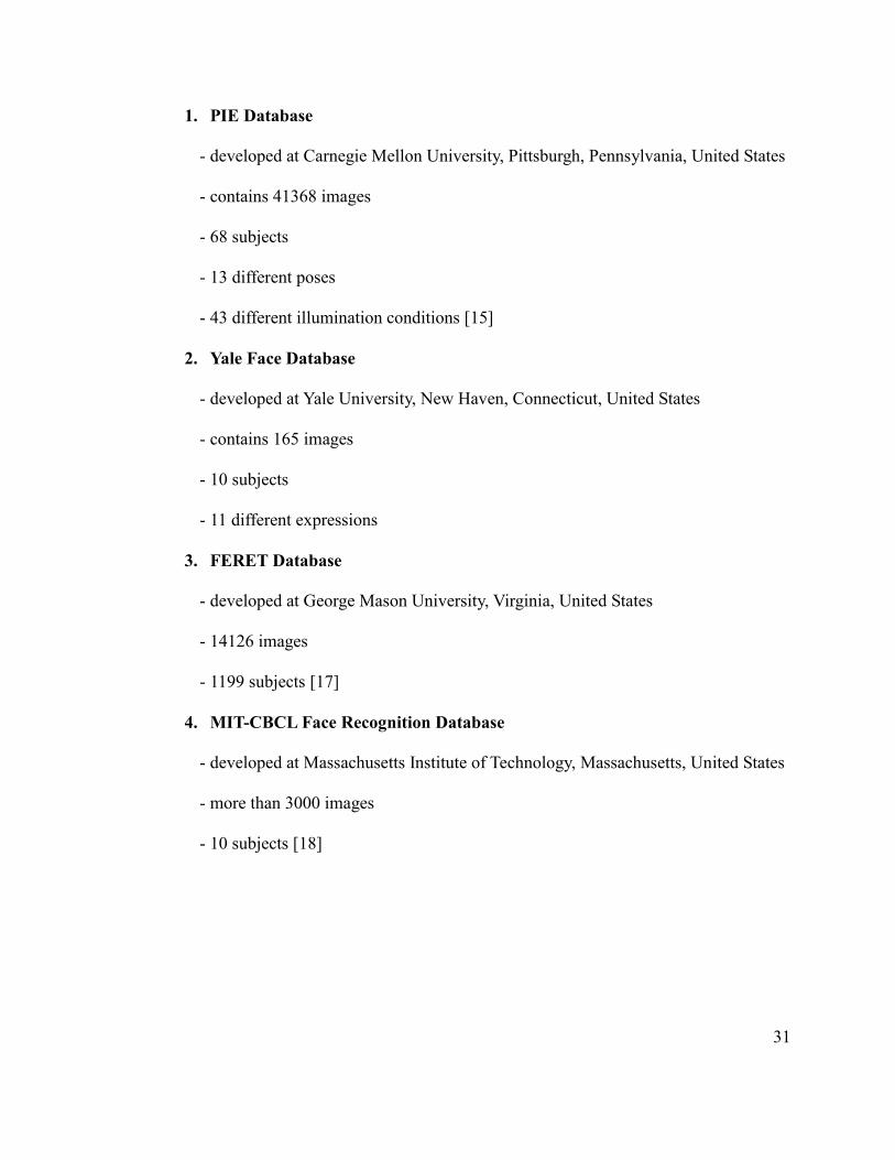
1. PIE Database
- developed at Carnegie Mellon University, Pittsburgh, Pennsylvania, United States
- contains 41368 images
- 68 subjects
- 13 different poses
- 43 different illumination conditions [15]
2. Yale Face Database
- developed at Yale University, New Haven, Connecticut, United States
- contains 165 images
- 10 subjects
- 11 different expressions
3. FERET Database
- developed at George Mason University, Virginia, United States
- 14126 images
- 1199 subjects [17]
4. MIT-CBCL Face Recognition Database
- developed at Massachusetts Institute of Technology, Massachusetts, United States
- more than 3000 images
- 10 subjects [18]

32
5. Face Recognition Data
- developed at University of Essex, England
- 7900 images
- 395 subjects
- 20 different images per individual [19]
6. M2VTSDB Database
developed at University of Surrey, England
- 333 images
- 37 subjects
- 5 different images per individual [20]
7. AR Face Database
- developed at Purdue University, Indiana, United States
- 4,000 images
- 126 subjects [21]
8. BioID Face Database
- developed by HumanScan AG, Switzerland
- 1521 images
- 23 subjects [22]
33
9. CalTech Faces Database
- developed by the Computational Vision Department at California Institute of
Technology, California, United States
- 450 images
- 27 subjects [23]
The above is just a brief description of the various databases commonly used in image
processing research, not all of the databases mentioned were utilized for the purposes of
this research. The section below gives an overview of the databases that were used in this
research.
3.1 Databases Utilized in this Research
This research aims to develop a tool for automatically analyzing the facial beauty in a
given image. In order to do so, as previously discussed, we have made the assumption
that beauty is viewed in a similar aspect across cultures. In order to remain consistent
with this assumption, this project utilizes images from databases containing images of
individuals from different ethnic backgrounds. Images from a total of five main databases
have been used for this research. The ethnicities incorporated in this research include
American, Latin-American, Asian, and European. The images for European individuals
include data taken from two databases, one containing images of British individuals and
another containing images of Dutch individuals. The Asian ethnicity was represented
through images from Chinese and Indian individuals. The following is a detailed
description of the images utilized for this research.
Normalization is an imperative step in the process of image processing, as it essentially
34
establishes consistency in the input images, hence being a critical component of ensuring
the validity and accuracy of results being obtained. Standardized and well processed
images also help improve the likelihood of success for any suggested approach.
The main focus in this research has remained on the analysis of human facial beauty in
females, therefore all the images utilized in this research are of females. It was necessary
to pre-process and normalize the images prior to their usage as inputs. Several steps were
necessary to ensure that all the images resulted in the same range of pixel intensity and
range of grayscale. The images were all resized and formatted to the dimensions of 800
pixels in height by 720 pixels in width and further converted to grayscale.
Some of the images in various databases had the subject wearing glasses or other facial
ornamentation. Such images were not used as the research focuses on images of females
with no facial ornamentation or device. All the subjects are also seen as having a forward
facing pose with a neutral expression. Furthermore, the subject's photo contains the head,
neck, and the top portion of the shoulders.
3.1.1 AR Face Database
The AR Face Database was compiled at Purdue University in the year 1998 by Aleix
Martinez and Robert Benavente. It was a joint collaboration by the two researchers from
different universities. Robert Benavente was studying at the Computer Vision Centre
Universitat Autonoma de Barcelona, while Aleix Martinex was studying at the Robot
Vision Lab at Purdue University. It is essentially a freely available public database which
was intended to help aid researchers in the areas of image processing and artificial
intelligence.
35
The database consists of images of a total of one hundred and sixteen people, with sixty
three of the images being of males and fifty three of the images being of females. Each
subject has thirteen different images; each image contains a different pose or setting of
the subject. The database contains images of Caucasian women, which includes women
of a European and North American background [21].
Some examples of poses include:
- neutral expression
- smile
- anger
- scream
- left light on
- right light on
- wearing sunglasses
- wearing a scarf
- wearing scarf and left light on
The pose used in the research included only the neutral pose. The calibration in pose,
illumination, and distance conditions of the images available from the database were
ideal for the analysis. A total of 35 images of females were used from the database. The
images used from the database were then resized to 800 pixels by 720 pixels and then
converted to grayscale.

36
Figure 6: Sample Images from AR Face Database
3.1.2 Psychological Image Collection at Stirling
Several of the databases included in this research are part of a large collection of facial
image databases at the University of Stirling in Scotland. Essentially meant as a public
database for use in the study of the psychology of faces, the entire collection of databases
is called the Psychological Image Collection at Stirling. There are a total of ten databases
containing frontal images of various subjects in numerous poses and situations. In
addition to these, the collection also includes two more databases which consist of images
of children's drawings and man-made objects respectively [27].
The databases from this collection that have been utilized in this research include:
- Stirling Faces Database
- Nottingham Faces Database
- Utrecht ECVP Database
3.1.2.1 Stirling Faces Database
The Stirling face database consists of mainly monochrome images, with a total of 312
images of thirty-five subjects. Eighteen of the respondents were female and the rest were
male, with each subject being photographed showing three different expressions and also
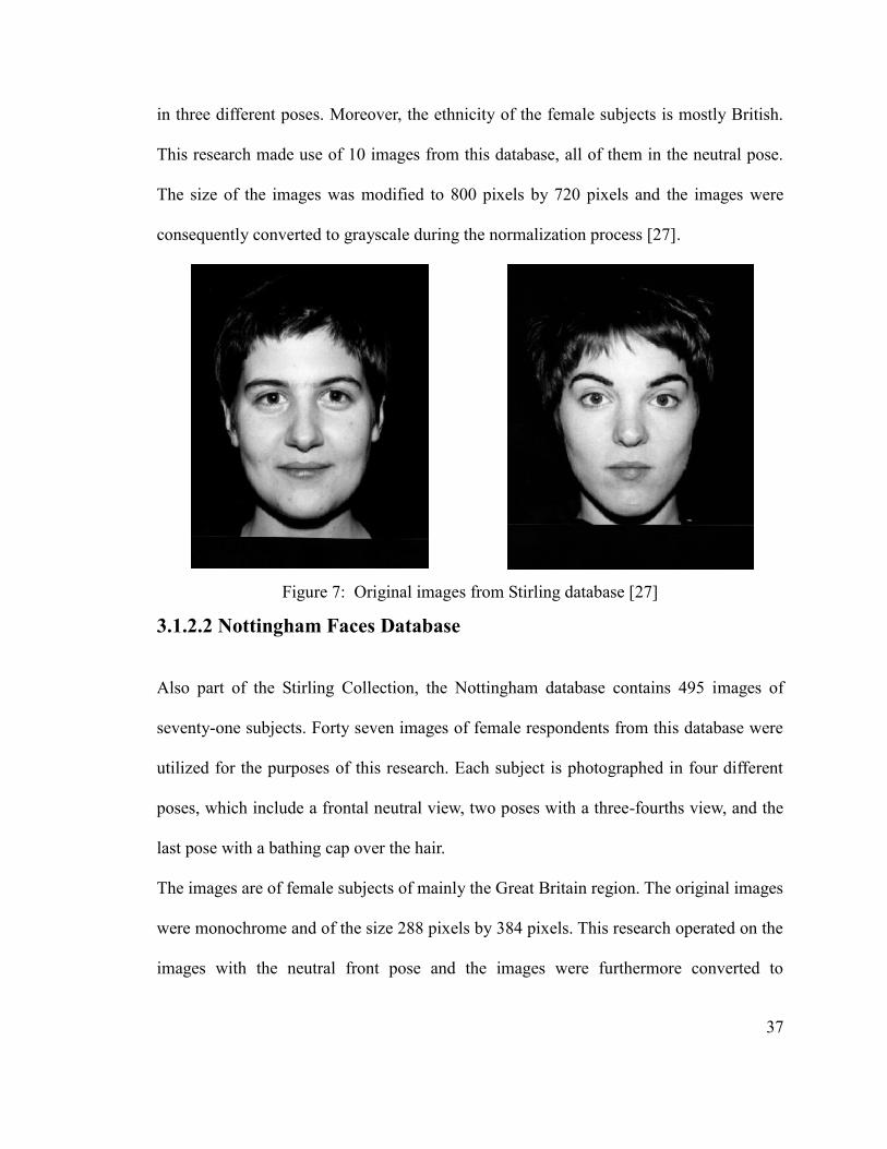
37
in three different poses. Moreover, the ethnicity of the female subjects is mostly British.
This research made use of 10 images from this database, all of them in the neutral pose.
The size of the images was modified to 800 pixels by 720 pixels and the images were
consequently converted to grayscale during the normalization process [27].
Figure 7: Original images from Stirling database [27]
3.1.2.2 Nottingham Faces Database
Also part of the Stirling Collection, the Nottingham database contains 495 images of
seventy-one subjects. Forty seven images of female respondents from this database were
utilized for the purposes of this research. Each subject is photographed in four different
poses, which include a frontal neutral view, two poses with a three-fourths view, and the
last pose with a bathing cap over the hair.
The images are of female subjects of mainly the Great Britain region. The original images
were monochrome and of the size 288 pixels by 384 pixels. This research operated on the
images with the neutral front pose and the images were furthermore converted to
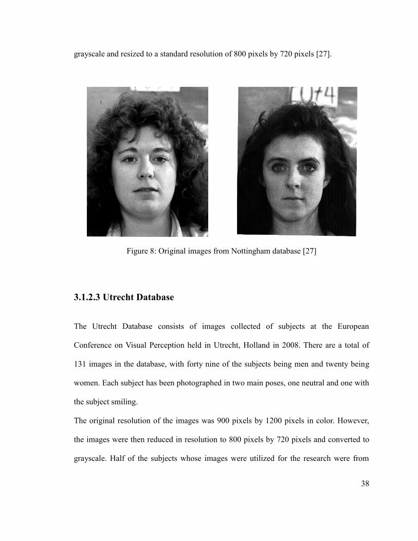
38
grayscale and resized to a standard resolution of 800 pixels by 720 pixels [27].
Figure 8: Original images from Nottingham database [27]
3.1.2.3 Utrecht Database
The Utrecht Database consists of images collected of subjects at the European
Conference on Visual Perception held in Utrecht, Holland in 2008. There are a total of
131 images in the database, with forty nine of the subjects being men and twenty being
women. Each subject has been photographed in two main poses, one neutral and one with
the subject smiling.
The original resolution of the images was 900 pixels by 1200 pixels in color. However,
the images were then reduced in resolution to 800 pixels by 720 pixels and converted to
grayscale. Half of the subjects whose images were utilized for the research were from
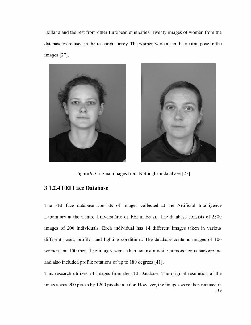
39
Holland and the rest from other European ethnicities. Twenty images of women from the
database were used in the research survey. The women were all in the neutral pose in the
images [27].
Figure 9: Original images from Nottingham database [27]
3.1.2.4 FEI Face Database
The FEI face database consists of images collected at the Artificial Intelligence
Laboratory at the Centro Universitário da FEI in Brazil. The database consists of 2800
images of 200 individuals. Each individual has 14 different images taken in various
different poses, profiles and lighting conditions. The database contains images of 100
women and 100 men. The images were taken against a white homogeneous background
and also included profile rotations of up to 180 degrees [41].
This research utilizes 74 images from the FEI Database, The original resolution of the
images was 900 pixels by 1200 pixels in color. However, the images were then reduced in
40
resolution to 800 pixels by 720 pixels and converted to grayscale. The images that were
used for this research had the subjects in the neutral pose.
3.1.2.5 Indian Face Database Beauty Queens
This database consists of face images taken of various subjects at the Indian Institute of
Technology, Kanpur, India. The images are taken of 40 distinct subjects comprising of a
total of 440 images in the database. These include 11 images taken for each of the 40
subjects as well as some additional photographs. The subjects are featured in various
orientations, which include facing front, facing left, facing right, facing up, facing up
towards left, and various others [42]. The subjects were also photographed displaying
several expressions such as sadness, happiness and a neutral expression.
This research utilizes 11 images from this database. The images were converted to a
resolution to 800 pixels by 720 pixels and subsequently converted to grayscale. The
images that were used for this research had the subjects in the neutral pose.
3.1.2.6 Images of Beauty Pageant Contestants
The final set of images used for the purposes of this research consisted of images sourced
from various publicly available databases containing images of beauty pageant
contestants. These images were of pageants from earlier years of the pageant and were
available for public use. The images used were taken from the Miss Universe and Miss
World pageants dating back to 2003. A total of 18 images were included in this research
to allow for representation of women that have been consciously selected for their beauty.
This helps to establish a more verified set of images for the ground truth set.

41
3.2 Survey Methodology
In order to establish the ground truths for this research, it was very important to collect
ratings from actual survey respondents. Thus, a survey was conducted and the results
collected and analysed for the purposes of establishing accuracy and consistency
standards for the research. The analysis also served the integral purpose of validating and
supporting the hypotheses and assumptions made in this research.
The hypotheses include the following:
- consistency in attractiveness ratings between male and female genders
- cross cultural consistency and correlation in attractiveness ratings
3.2.1 Participants for the Survey
In this research, a survey was conducted, for the purposes of collection of attractiveness
ratings, on several data sets of facial images of females. The volunteers consisted of a
total of 48 people. Many of the participants were in the age group of 20 to 30 years. The
volunteers were chosen so as to represent many diverse cultures and ethnic backgrounds
and therefore the set consists of respondents from various countries.
Volunteers included 12 people of White Canadian background, which were made up of 4
men and 8 women. Furthermore, respondents included 4 females and 4 males of Chinese
background, 4 females and 3 males of a Hispanic background, 4 females and 4 males of
an Indian background, 3 females and 5 males of a British background, as well as 3
females and 2 males of a Japanese background. The data associated with the respondents,
including the background, average age ranges, and etc. is shown in Table 2.

42
Respondent Background Average Age Number of Females Number of Males
White Canadian 24 8 4
Chinese 24 4 4
Hispanic 25 4 3
Indian 23 4 4
British 25 3 5
Japanese 23 3 2
Table 2: Data related to the Survey Participants
The scope of the survey included participants of various backgrounds. A great number of
the participants were international students at the university. This was of importance as
they had exposure to both their own cultural conceptions of beauty and had, in addition,
also been in contact with people from various backgrounds after having arrived in
Canada. Thus, the respondents possessed experience and knowledge to make an informed
decision with regard to the survey. Several of the students were also living in other
countries abroad; this had the effect of making the respondent population diverse and
accounted for variations in beauty preferences.
3.2.2 Data Set
Two hundred and fifteen gray scale photographs were used for the purposes of this
survey. The photographs were presented in a grid format, with each photograph taking up
one block of a 25 x 20 cm grid, with each block of size 4 x 3 cm. The data set consisted
of images from several publicly available databases, with each database containing
images of women from a different ethnic background. Thirty five images were used from
43
the AR face database, which contains mainly images of Caucasian women. A further
forty-seven images were used from the Nottingham Face Database, which consists of
images from women in Great Britain. Seventy four images were taken from the FEI
Database, which contains images of women of Hispanic and Latin-American
backgrounds. Twenty images were taken from the Indian Face Database, and ten images
were selected from the Utrecht Face Database which contained images from several
European countries. In addition to these images, a further twenty nine images were also
added to the data set; these images were of women that had participated in beauty
pageants from various countries around the world.
The variation in these images provides the desired group of images from an international
sample of people. The mean age of the participants was centered around 24 years. The
women in each image had a neutral face expression and did not wear glasses or any facial
ornamentation. The images only revealed the face and the tops of the shoulders.
3.2.3 Procedure and Ratings Collection
Each respondent was provided with the entire collection of images, with the images
randomly organized on an image grid. Individual respondents were provided with clear
instructions regarding the survey methodology and purpose of research and were
informed that their personal data would not be released. They were requested to examine
and quickly scan all the images in the data set. Having done that, they were then asked to
assess each image on the basis of facial attractiveness of each subject, being told
specifically not to be biased by race or ethnicity. In addition, they were informed that
their decision should be based on facial factors such as beauty and aesthetic factors.

44
The ratings were based on the Likert psychometric scale, which is designed explicitly for
the validation and measurement of such personality traits and is often utilized for the
purposes of psychometric surveys such as this. In this research, the use of a five-point
Likert scale was decided upon, ranging from attractive being denoted by 5 on the scale to
unattractive being denoted by 1. Each respondent was asked to fill out the rating box
below each image with the corresponding rating that was decided upon.
Figure 10: An excerpt from the survey
The scale used to rate the images is as follows:
1. unattractive
2. below average
3. average
4. above average
5. attractive
Several tendencies exist in respondents that this research tried to eliminate. These include
a tendency of respondents to assign average marks in order to avoid offense to subjects.
In order to eliminate this potential source of discrepancy, the respondents were informed

45
that their ratings were confidential and would not be released to the general public.
Furthermore, many respondents were not sure what exact traits each rating corresponds
to; this was eliminated by giving an explicit description associated with each rating.
Attractiveness Rating Percentage of Images
5 17.2
4 22.6
3 22.2
2 20.9
1 17.2
Table 3: Percentage of Images at each Level of Attractiveness
3.2.4 Ratings Analysis
The analysis of attractiveness ratings is particularly essential as it allows for the
validation and testing of several hypotheses and assumptions held in this research.
Moreover, it provides significant correlations between attractiveness ratings and certain
facial characteristics.
Two main assumptions regarding beauty and attractiveness were held during this
research, the first one being that there exists a consistency in attractiveness ratings
between the male and female genders. Secondly, it was also integral to the basis of this
research that there exist a general agreement in between various cultures and ethnicities
over beauty and attractiveness.
In order to test these assumptions, ratings were collection and analyzed for correlations
and consistencies. These correlations are useful because they help in establishing patterns
that can help establish a predictive relationship, which in turn can be used as the basis of

46
several experiments and research.
It was found that there was a strong correlation between the ratings of White Canadian
males and females, with a correlation of r=0.89. There was also a strong correlation of
ratings between most of the ethnic backgrounds except for the Indian respondents, for
which the correlation was slightly lower than the rest of the population of respondents.
Furthermore, cross-cultural correlations were analyzed for any significant results. This
was done by analyzing the attractiveness ratings and calculating the mean ratings for the
ratings given to an image by participants of a particular nationality or ethnic background.
The findings are displayed below. The mean correlation between the groups was around
0.86, with a strong correlation in ratings between the white Canadian, British, Chinese
and Indian respondents. There was a slightly lower correlation between the ratings of the
Thai respondents and the rest of the respondent population.
Table 3 shows the percentage of images that were rated for each level of attractiveness
ratings. The ratings are relatively normally distributed.
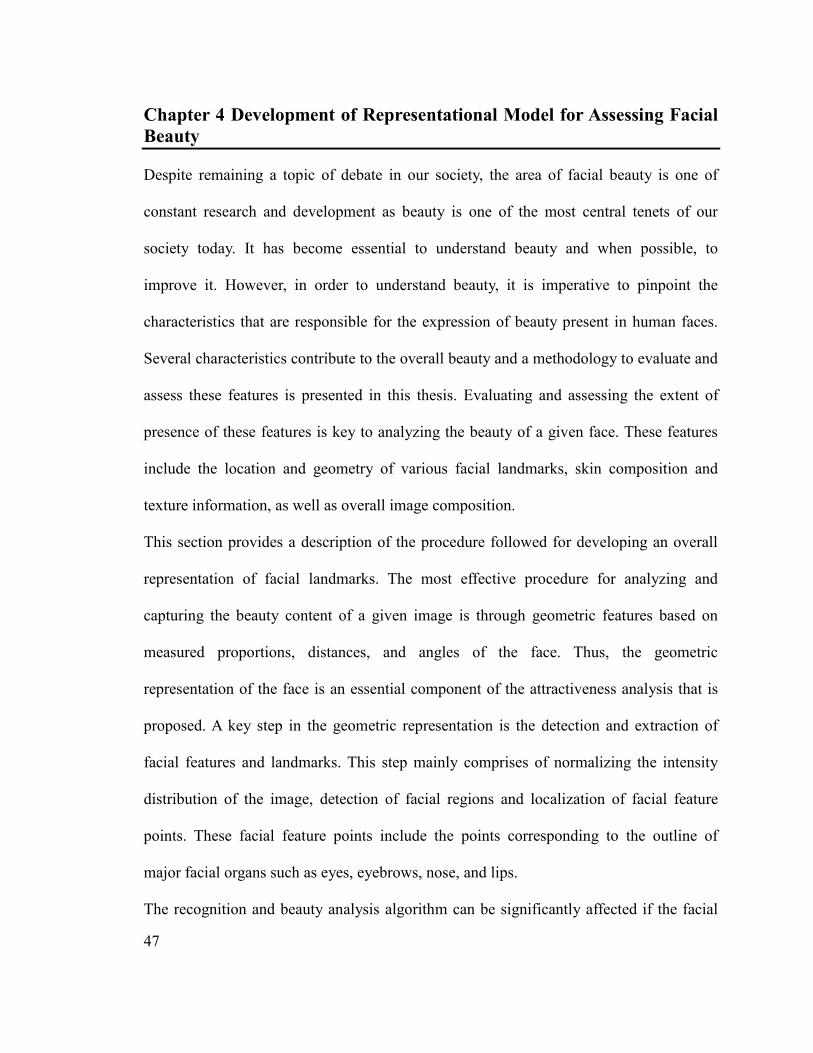
47
Chapter 4 Development of Representational Model for Assessing Facial
Beauty
Despite remaining a topic of debate in our society, the area of facial beauty is one of
constant research and development as beauty is one of the most central tenets of our
society today. It has become essential to understand beauty and when possible, to
improve it. However, in order to understand beauty, it is imperative to pinpoint the
characteristics that are responsible for the expression of beauty present in human faces.
Several characteristics contribute to the overall beauty and a methodology to evaluate and
assess these features is presented in this thesis. Evaluating and assessing the extent of
presence of these features is key to analyzing the beauty of a given face. These features
include the location and geometry of various facial landmarks, skin composition and
texture information, as well as overall image composition.
This section provides a description of the procedure followed for developing an overall
representation of facial landmarks. The most effective procedure for analyzing and
capturing the beauty content of a given image is through geometric features based on
measured proportions, distances, and angles of the face. Thus, the geometric
representation of the face is an essential component of the attractiveness analysis that is
proposed. A key step in the geometric representation is the detection and extraction of
facial features and landmarks. This step mainly comprises of normalizing the intensity
distribution of the image, detection of facial regions and localization of facial feature
points. These facial feature points include the points corresponding to the outline of
major facial organs such as eyes, eyebrows, nose, and lips.
The recognition and beauty analysis algorithm can be significantly affected if the facial

48
points are located inaccurately. Therefore it is of the utmost importance to choose an
algorithm that locates facial features and landmarks with a great level of accuracy. Other
challenges that may be faced include images with resampling artifacts and external
objects such as eyeglasses, hands, and jewelry.
Deformable models, a methodology used mainly for representing objects in the field of
computer vision, were used to accurately represent faces in this research. Having been
used in various fields for shape representation, this technique basically utilizes a set of
known objects to analyze digital images. The main methodology is based upon
approximation and geometry for the analysis.
In the context of this research, two main models were examined, these include Active
Shape Models and Active Appearance Models. The Active Shape Model essentially tries
to match a given set of points to an image using a statistical shape model, whereas the
Active Appearance Model matches the position and texture of model points related to an
image [45].
The algorithm for development of the facial representation is based on the Active Shape
Model concept. Active Shape Models uses an iterative technique to match model points
to a new image, which involves searching around each point to find a point nearby which
best matches the model expected around that point. Then, the parameters which control
point positions are adjusted in order to move the point closer to match the location of
point in the image. The Active Appearance Model, on the other hand, generates a model
of appearance which represents shape variation in the image, and then uses the
differences between the current image model and target image to adjust its parameters
[45].

49
The accuracy of both models was tested with various data sets. The results obtained with
both models were compared with actual hand labeled points. For the data used in the
scope of this research, the Active Shape Model located facial points with greater
accuracy. In addition, the Active Shape Model also had a slightly lower runtime. The
Active Appearance Model has a slightly larger capture range but the results become
comparably better for the Active Shape Models as resolution is increased.
The methodology used in this research focuses on a specific deformable model technique
known as Active Shape Models, developed by Cootes et al. The following chapter
provides a brief overview of the procedure followed [45].
4.1 Active Shape Models
This section examines Active Shape Models and explains the main concepts and
methodology followed in this research. Given an image of a face, the Active Shape
Model essentially aids in the positioning of landmarks. Active Shape Models are
essentially statistical models of given objects. When given an image of a new object,
these models iteratively deform to fit to that object [45]. A training set containing labeled
images is provided to the models and the shapes can only vary as much as and in ways
that are seen in the training set. After the model is trained, the search for the features
occurs.
4.2 Shapes
In the context of this research, a shape is essentially a set of landmarks on the face, which
would be an array of x and y coordinates. Any Euclidean transformation such as an
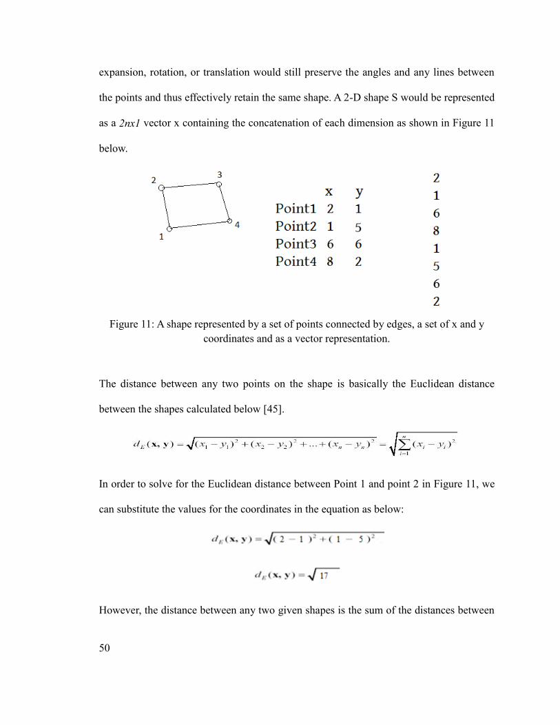
50
expansion, rotation, or translation would still preserve the angles and any lines between
the points and thus effectively retain the same shape. A 2-D shape S would be represented
as a 2nx1 vector x containing the concatenation of each dimension as shown in Figure 11
below.
Figure 11: A shape represented by a set of points connected by edges, a set of x and y
coordinates and as a vector representation.
The distance between any two points on the shape is basically the Euclidean distance
between the shapes calculated below [45].
In order to solve for the Euclidean distance between Point 1 and point 2 in Figure 11, we
can substitute the values for the coordinates in the equation as below:
However, the distance between any two given shapes is the sum of the distances between

51
their corresponding points. The Procrustes distance between two shapes is the root mean
square distance between the shape points.
4.3 Landmarks
The various features of interest in each image are called landmarks. Landmarks are
usually chosen at clear corners of object boundaries, such as 'T' junctions between
boundaries or biological landmarks.
Formally defined, “a landmark is a point of correspondence on each object that matches
between and within populations”.
There are three main types of landmarks, which include anatomical landmarks,
mathematical landmarks, and pseudo-landmarks. Anatomical landmarks have biological
significance across organisms and are assigned by an expert. Mathematical landmarks are
assigned to objects due to some mathematical property. The overall shape is represented
by recording the connectivity between the landmarks to define how the landmarks join to
form the boundaries of the shape.
Given landmarks labeled . We can thus represent the n
points as a single 2n element vector, x, where = . Given that we
have P training examples, we will generate p such vectors xj. Before any further analysis,
the shapes must be all represented in the same coordinate frame [45].
4.4 Shape Alignment
To obtain a true representation of the shape, any effects due to location, scale, and
rotational transformations need to be filtered out. In order to do this, a coordinate
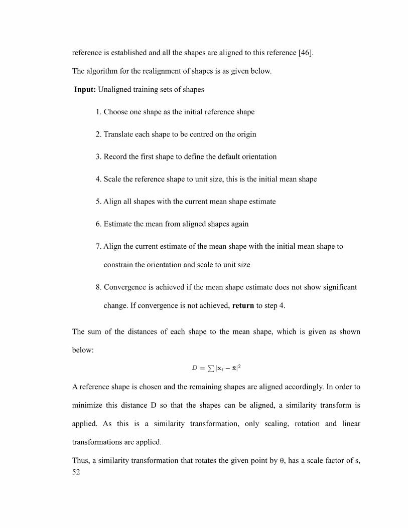
52
reference is established and all the shapes are aligned to this reference [46].
The algorithm for the realignment of shapes is as given below.
The sum of the distances of each shape to the mean shape, which is given as shown
below:
A reference shape is chosen and the remaining shapes are aligned accordingly. In order to
minimize this distance D so that the shapes can be aligned, a similarity transform is
applied. As this is a similarity transformation, only scaling, rotation and linear
transformations are applied.
Thus, a similarity transformation that rotates the given point by θ, has a scale factor of s,
Input: Unaligned training sets of shapes
1. Choose one shape as the initial reference shape
2. Translate each shape to be centred on the origin
3. Record the first shape to define the default orientation
4. Scale the reference shape to unit size, this is the initial mean shape
5. Align all shapes with the current mean shape estimate
6. Estimate the mean from aligned shapes again
7. Align the current estimate of the mean shape with the initial mean shape to
constrain the orientation and scale to unit size
8. Convergence is achieved if the mean shape estimate does not show significant
change. If convergence is not achieved, return to step 4.

53
and an applied translation is as follows [46]:
The shape is scaled by shrinking the size while preserving shape proportions. In addition,
translation allows the shapes to have a common center, by moving each shape to its
origin and subtracting the mass center of each point.
For the final step, we need to apply a rotation matrix, which in turn requires the
calculation of a Singular Value Decomposition (SVD). The Singular Value
Decomposition of a matrix is the decomposition of a given matrix = UDVT
, such that V is
the eigenvector of ATA and U is the eigenvector of AA
T [46]. For the rotation matrix of
shape xi in terms of xj, the SVD of xiTxj is needed. The rotation matrix is then calculated
as follows:
= [cosθ − sinθ
sinθ cosθ ]
The Active Shape Model (ASM) is trained on a set of manually landmarked images
before training begins. After the training, the ASM is used to search for features on a
face. The general approach is to try to locate the landmarks independently and then
correct the locations by observing the relationship between the landmarks' locations [46].
The ASM is constructed from two main sub-models: the profile model and the shape
model. The shape model acts globally, while the profile model acts locally.
4.5 Profile Model
The profile model specifies what the overall image is supposed to look like around a
54
particular landmark on a given face. Its main task is to formulate a shape for a given face
approximation by template matching at the landmarks.
The profile model is based on profile vectors, which are one-dimensional vectors which
describe the characteristics of the image around a given landmark. The area around each
landmark is sampled in order to build a profile model for the particular landmark, after
sampling the vector is then again moved to the position that best corresponds to the
landmark's model profile.
The profile vector g at a given landmark is formed by sampling intensities along a one-
dimensional vector which is orthogonal to the shape edge. This vector is often referred to
as a whisker, as it is a small vector containing a small set of intensities found in the
neighborhood of a shape edge. This is illustrated in Figure 12 below [47].
Figure 12: Example of construction of profile vector
The yellow line represents the edge of a particular shape. The gray line orthogonal to the
edge is the whisker; the landmark is located at the intersection of the two lines. The
profile vector is derived from the whisker vector at the boundary and after going through
55
a set of normalization steps, contains the values desired.
The profile vector, g, is formed through a set of steps. Initially, the elements of the profile
vector are set to the intensity values of the image below it. Then, each profile element is
replaced with the value found by calculating the difference between its own value and the
value of the previous element. Each element is then divided by the sum of the absolute
values of all vector elements. These normalized gradients have the effect of lessening
varying image lighting and contrast [47].
4.6 Shape Model
The ASM shape model essentially defines the allowable positions of landmarks. This
model helps to adjust the shape suggested by the profile model to match a legitimate face
shape, making this an integral component because profile matches at landmarks are often
unreliable. Before building the model, it is important that the shapes be aligned.
The shape model is made up of two components: the average face and the allowable
distortions on the average face [46]. This is represented by the following equation:
The mean shape is defined as follows [46]:
Here is the shape vector generated by the model, is the average of the aligned training
shapes xi, and Φ represents the matrix of eigenvectors of the covariance matrix S of the
training shape points [47].

56
The covariance matrix is calculated as follows:
Thus the equation [top of page] can be used to model different shapes by varying the
main vector parameter b. By ensuring that the values of b fall within known limits, the
model generates lifelike faces. The limits fall between and , where λi is the
ith eigenvalue of S. Figure 13 below shows the generated mean face shape model
represented with the solid black line and the several variations on the shape model
represented with gray lines [45].
Figure 13: The mean face shape model (black line) and the variations on the model (gray
lines)
4.7 ASM Image Search
After the completion of the models, they can be used to located regions of faces in new
input images. Cootes et al [47] defined an algorithm to find the adapted shape x, given a
target shape y, by fitting the constructed model to the new set of points [47]. During
this search, several searches are constructed by sampling the image in the neighborhood
57
of each landmark. The algorithm for ASM Search is as follows:
Input : Face Image
1. Generate the start shape by locating the overall position of the face
2. Sample the area around the offset to build a profile and measure the fit of the
profile against the profile model built
3. Move the point to the offset of the best profile match
4. Adjust the suggested shape to conform to the Shape Model
5. Repeat until convergence, which means until no further improvements are
possible
Output: Shape with (x,y) coordinates of face landmarks [46].
4.8 Fitting Generated Model to Given Points
The key parameter used to build a given model is b, which is the shape parameter. One
specific value of b corresponds to one specific form of the model, which can be turned
into the corresponding shape by using the transformation from the model's coordinate
frame to the image's frame. In order to fit a particular model to new points, we must first
initialize all the shape parameters to zero.
Any instance of the model is represented by
.
The model instance is then generated and the set of parameters that minimizes ∆x is
computed and is given by y-T(x)2. Here T is the similarity transformation described
below:
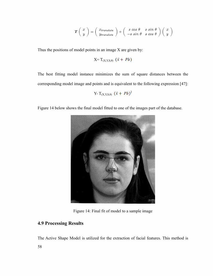
58
Thus the positions of model points in an image X are given by:
X= T(X,Y,S,θ)
The best fitting model instance minimizes the sum of square distances between the
corresponding model image and points and is equivalent to the following expression [47]:
Y- T(X,Y,S,θ) 2
Figure 14 below shows the final model fitted to one of the images part of the database.
Figure 14: Final fit of model to a sample image
4.9 Processing Results
The Active Shape Model is utilized for the extraction of facial features. This method is

59
quite efficient in locating various landmarks on the face and being able to extract the
position of the corresponding landmark. However, the input needs to be an image with a
good resolution quality as the output of the algorithm is greatly improved when image
quality improves. The processing contains errors when the image is not of a consistent
variation such as when the person is wearing glasses.
Furthermore, the training of the model is highly dependent on the initial landmarks input
into the algorithm. Therefore, the accuracy is often constrained by the initial precision of
landmark placement. After running the algorithm for several variations of inputs, the best
results were obtained with images of a resolution of 800 by 720 pixels. The convergence
of the algorithm occurred after 17 iterations for the final run of inputs. With an overall
likelihood of error occurring for around 2 percent of images, the algorithm provided
generally consistent results.
60
Chapter 5 Formulation of Algorithm for Beauty Analysis
Feature selection is one of the most important steps that affect the accuracy of analysis.
The selection of features is dependent upon what characteristics play a role in the
formulation of a representation that exemplifies the integral components of human
beauty. This determines the validity and accuracy of results. In the scope of this research,
the features used have been chosen to develop an effective representation of the essential
components of the human face. The main challenge has been in selecting what aspects of
the human face inherently contribute to the perception of beauty. The challenge has been
in the quantification of the identification of beauty.
Various theories of beauty exist in order to aid the understanding of this concept. The
geometric representation of a face often helps to identify the key components of a given
face. In addition to this the texture of a face is of importance in relation to beauty.
Furthermore, the overall shape of the face must be represented as well in order to
complete the description.
This chapter outlines the overall implementation and methodology proposed by this
research. The proposed algorithm represents the face using various key characteristics.
The features extracted help to represent facial characteristics in three major areas.
Geometric features help to represent the symmetrical properties and ratio-based
properties of landmarks on the face. Textural features extracted help capture information
related to skin texture and composition. Finally, face shape and outline features help to
categorize the overall shape of a given face, which helps to represent the given female
face shape and outline for the further analysis of any deviations from the basic face
shapes. The algorithm is made up of sub-modules for each of these sets of features. Each

61
module has been developed as part of this research and is a novel contribution. The
system is outlined in Figure 28, which shows the significant components and steps
followed to establish the system.
5.1 Facial Representation
Beauty analysis is highly dependent upon the representation of the face that is provided to
the classifier. The more realistic the representation, the more accurate the results will be.
Hence, the chosen features must be accurate and integral components of the real world
representation of beauty and of the processed data as well.
In the approach of this research, the Active Shape Model is proposed for the extraction of
facial landmarks, which has resulted in an accurate set of landmarks and their positions.
The Active Shape Model algorithm is used as the foundation of the overall algorithm
developed for extracting the major landmark positions. The Active Shape Model concept
was adapted for accurate analysis of facial features, thus the algorithm was developed
using the model. The model obtained was then trained specifically for the databases
utilized in this research.
After extracting the positions of landmarks, the feature vector must be prepared for
training purposes. The contents of the feature vector depend on the combination of beauty
analysis algorithms. This research proposes an accurate representation of natural facial
beauty. This involves the geometric representation of facial landmarks, texture analysis,
as well as edge histogram information.
In order to extract features from a given image, it is often important to locate key
landmarks on the image in order to further process those landmarks for the formation of
62
features.
The model was initially trained on the Nottingham Face Database, as it was an accurate
representation of the resolution and size of the other datasets in the research.
For detecting parameters using this model, it is important to align them in order to obtain
good results. The process has been outlined in detail in Chapter 4. However, the
following explanation presents a brief summary. The main steps taken for the alignment
are as follows:
1. Selection of reference shape, letting
2. Translation of each shape to centre it on origin, , which is essentially
for pose correction.
3. Scale reference shape to unit size
4. Recalculate mean shape from aligned shapes
5. Constrain mean shape and align
6. Iterate until convergence
After the alignment of the training set has occurred, the shape must be modeled. The
mean shape and the covariance matrix are computed from the aligned training set
by the application of Eq 5.1:
(5.1)
The covariance matrix is computed as follows:
(5.2)
As demonstrated earlier, the shape model is represented as . Here x is the
shape vector generated, is the set of eigenvectors of the covariance and b
63
represents the parameter for the shape vector.
The final step involves fitting the model that has been constructed to a new set of points,
which can be represented by z. Each shape has its own characteristic parameter b, which
is set to zero when first fitting a set of points. Thus, the following steps are further
followed:
1. Model instance is represented by
2. Find parameters which best align model points, parameters include:
3. Invert the transformation of T(y) to get
4. Update the parameter of b and apply constraints.
5. Iterate until convergence [46]
These steps are necessary for fitting the new set of points to an already existing model.
Figure 13 shows the results of the various iterations performed until a fit is achieved. For
each image, the landmarks were initially detected directly on the image itself, and then
the map of labeled points was scaled to a coordinate system. Finally, a computer
application was programmed to compute each of the measurements associated with the
geometric feature vector.
5.2 Geometric Features
Geometric features play a key role in the analysis of the beauty content of a face. In order
to extract the geometric features, each face had to be landmarked. The landmarking
process required images to be of a certain quality in order for the results to be of the
highest accuracy. Various image sizes were experimented with in order to find the size
that resulted in most accurate feature extraction. The size that was found to result in the

64
best extraction results was 800 pixels by 720 pixels. Table 4 below shows the various
sizes tested and their respective results.
Size Accuracy Results (%)
450 pixels by 350 pixels 68.3
640 pixels by 560 pixels 77.1
800 pixels by 720 pixels 85.0
Table 4: Sizes tested with their corresponding results
Various geometric features were extracted from each face in order to form an accurate
representation. The extraction of features was implemented in C. The focus was on
choosing features that would result in the highest accuracy when testing with the sample
data set. After undergoing several tests, a feature vector containing the select features
which effectively described the feature set was constructed. The following sections will
describe in further detail the various components of the features vector.
A total of 62 landmark points were selected for each facial image. The landmark points
contained various sub categories corresponding to regions of the face. For example, a
total number of 15 points represented the outer outline of the face, 6 points represented
each eyebrow, etc; these are illustrated in the diagram outlined in Figure 15.
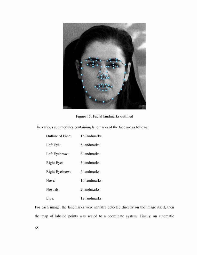
65
Figure 15: Facial landmarks outlined
The various sub modules containing landmarks of the face are as follows:
Outline of Face: 15 landmarks
Left Eye: 5 landmarks
Left Eyebrow: 6 landmarks
Right Eye: 5 landmarks
Right Eyebrow: 6 landmarks
Nose: 10 landmarks
Nostrils: 2 landmarks
Lips: 12 landmarks
For each image, the landmarks were initially detected directly on the image itself, then
the map of labeled points was scaled to a coordinate system. Finally, an automatic
66
computer application was generated to compute each of the measurements associated
with the geometric feature vector. The final results of this application were then analyzed
for the purposes of inclusion in the final feature vector.
5.2.1 Ratios Pertaining to Major Facial Regions
The combination of features from various theories of facial beauty makes the proposed
algorithm unique. The algorithm for the geometric features sub-module has two main
parts. The first section contains basic measurements taken of various regions of the face,
while the second section extracts features based on various theories of beauty.
This section elaborates on the basic measurements taken of various regions of the face.
Section 5.2.2 will elaborate further on the features associated with various theories of
beauty.
The first set of ratios to be discussed mainly involves ratios extracted from the major
facial regions. These regions include the eye region, the nose region, and the mouth
region. Each region was analysed and a number of associated measurements and ratios
were extracted for each respective region. The following sections help to outline these
measurements.
5.2.1.1 Eye Features
Before coming up with the final set of feature vector for the eyes, several combinations of
features were experimented with. Initially, the overall size of the eye was represented in
terms of the landmark points that formed the outline of the eye. This effectively meant
that rather than calculating the width or height at only a certain point of the eye, all the

67
points that were part of the outline of the eye were taken into consideration. Using this set
of points as part of the final training vector, the classification results demonstrated an
accurate classification percentage of around 67%.
Figure 16: Detailed diagram of eye [56]
It was evident that this number could definitely be improved upon. The features that were
used next for the vector consisted of specific distances that were measured for various
parts of the eye. Some of the specific measurements that were extracted are shown below
in the table; these are mainly relationships between the iris, pupil, and corners of the eye.
In addition to this, the relationships between the eye and its surrounding facial features
were also considered; these included relationships between the eye and the eyebrow, the
eye and mouth corners, the eye and the nose tip, the eye and the face outline [56].
The table below, Table 5 outlines the various features that were used from the eye. In
order to make the descriptions more clearly, Figure 16 illustrates the various
terminologies and parts of the eye mentioned in Table 5.
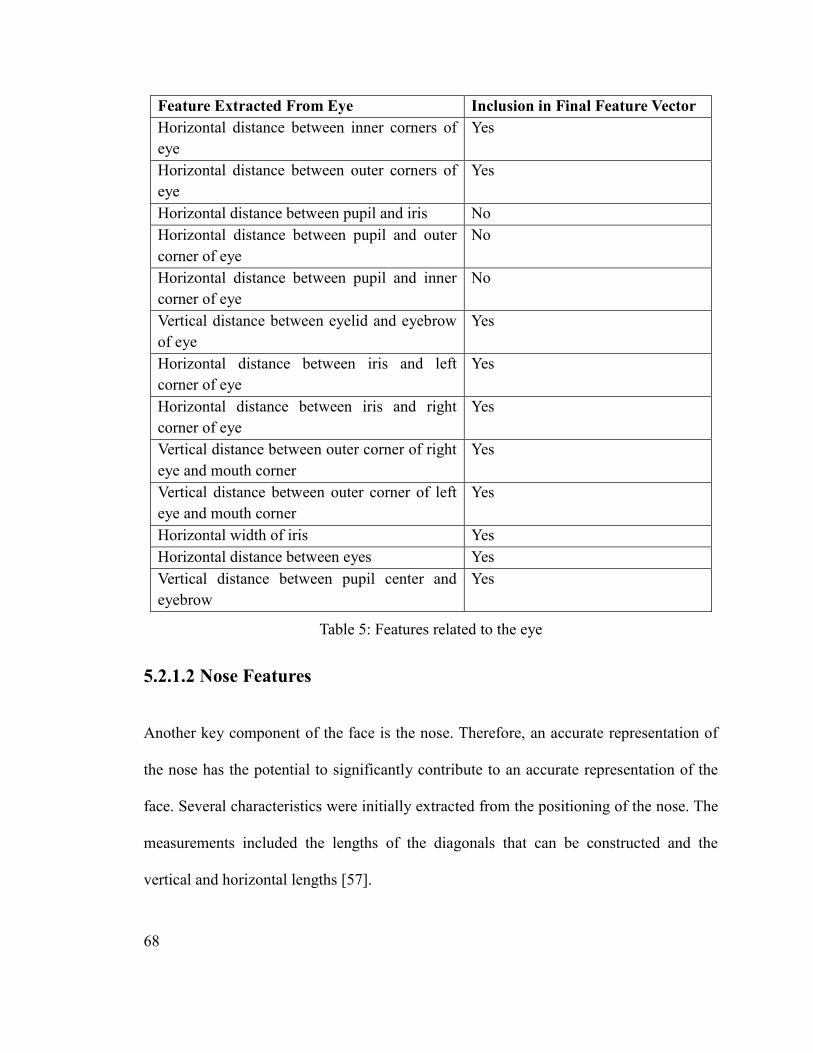
68
Feature Extracted From Eye Inclusion in Final Feature Vector
Horizontal distance between inner corners of
eye
Yes
Horizontal distance between outer corners of
eye
Yes
Horizontal distance between pupil and iris No
Horizontal distance between pupil and outer
corner of eye
No
Horizontal distance between pupil and inner
corner of eye
No
Vertical distance between eyelid and eyebrow
of eye
Yes
Horizontal distance between iris and left
corner of eye
Yes
Horizontal distance between iris and right
corner of eye
Yes
Vertical distance between outer corner of right
eye and mouth corner
Yes
Vertical distance between outer corner of left
eye and mouth corner
Yes
Horizontal width of iris Yes
Horizontal distance between eyes Yes
Vertical distance between pupil center and
eyebrow
Yes
Table 5: Features related to the eye
5.2.1.2 Nose Features
Another key component of the face is the nose. Therefore, an accurate representation of
the nose has the potential to significantly contribute to an accurate representation of the
face. Several characteristics were initially extracted from the positioning of the nose. The
measurements included the lengths of the diagonals that can be constructed and the
vertical and horizontal lengths [57].
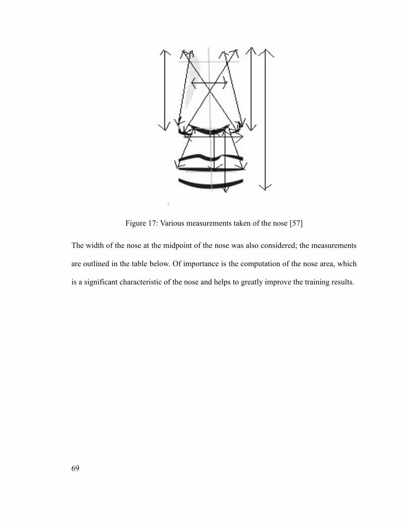
69
Figure 17: Various measurements taken of the nose [57]
The width of the nose at the midpoint of the nose was also considered; the measurements
are outlined in the table below. Of importance is the computation of the nose area, which
is a significant characteristic of the nose and helps to greatly improve the training results.
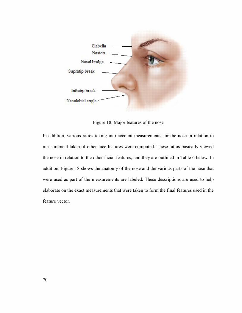
70
Figure 18: Major features of the nose
In addition, various ratios taking into account measurements for the nose in relation to
measurement taken of other face features were computed. These ratios basically viewed
the nose in relation to the other facial features, and they are outlined in Table 6 below. In
addition, Figure 18 shows the anatomy of the nose and the various parts of the nose that
were used as part of the measurements are labeled. These descriptions are used to help
elaborate on the exact measurements that were taken to form the final features used in the
feature vector.

71
Feature Inclusion in Final Feature Vector
Horizontal distance between two nostrils Yes
Horizontal width of protrusion of nose Yes
Vertical length of nose from glabella to infratip Yes
Nose area Yes
Vertical length between glabella to bottom edge
of lower lip
No
Diagonal length from the nasion to right nostril
of nose
No
Diagonal length from the nasion to left nostril
of nose
No
Diagonal length from the left nostril to left
corner of mouth
Yes
Diagonal from the right nostril to right corner
of mouth
Yes
Table 6: Ratios related to the nose
5.2.1.3 Mouth Area Features
The last component of the face that was analyzed was the mouth area. This area consists
mostly of the lips; the relationship between the lips and the rest of the face is also
observed. The landmarks forming the outline of the lips were located and they form part
of the feature vector. In addition to these, several other features associated with the lips
were extracted. These include the thickness of the upper and lower lip, the horizontal
length of the lip, various ratios pertaining to the lip in relation to other facial features. The
ratios and other major features are presented in Table 7 below.

72
Figure 19: Landmarks of the mouth
When analyzing the features related to the lips, it was important to eliminate some
features that did not contribute effectively to the feature vector and in some cases
decreased the accuracy of the representation [58]. Features that were eliminated included
the midpoints of the lips and line representing the division between the upper and lower
lip. The landmarks of the mouth that were part of the feature vector are illustrated in
Figure 19. Consequently, these landmark names are used to further describe the ratios in
Table 7 which were obtained for the final feature vector.

73
Feature
Inclusion in Final
Vector
Vertical distance between oral commisure to center of face Yes
Vertical thickness of upper lip= difference between length
from nose until oral commisure and length from nose until
upper lip vermillon border
Yes
Vertical thickness of lower lip= difference between length
from nose until oral commisure and length from nose until
lower lip vermillon border
Yes
Vertical distance between upper lip vermillon border and chin No
Vertical distance between lower lip vermillon border and chin Yes
Vertical distance between nose tip and upper lip vermillon
border = Philtum
No
Lip area of upper lip = total skin area of upper lip No
Lip area of lower lip = total skin area of lower lip No
Table 7: Ratios related to the mouth
5.2.2 Ratios Pertaining to Facial Beauty Theories
The representation of facial beauty is based on several maxims of beauty that have been
established over the years. The Golden Ratio and Facial Thirds methods have been used
when formulating a geometric representation. In addition to these methods, five more
ratios have been added that have improved the representation of the face greatly. This
has even led to various plastic surgeons and scientists applying these methods to their
practices.
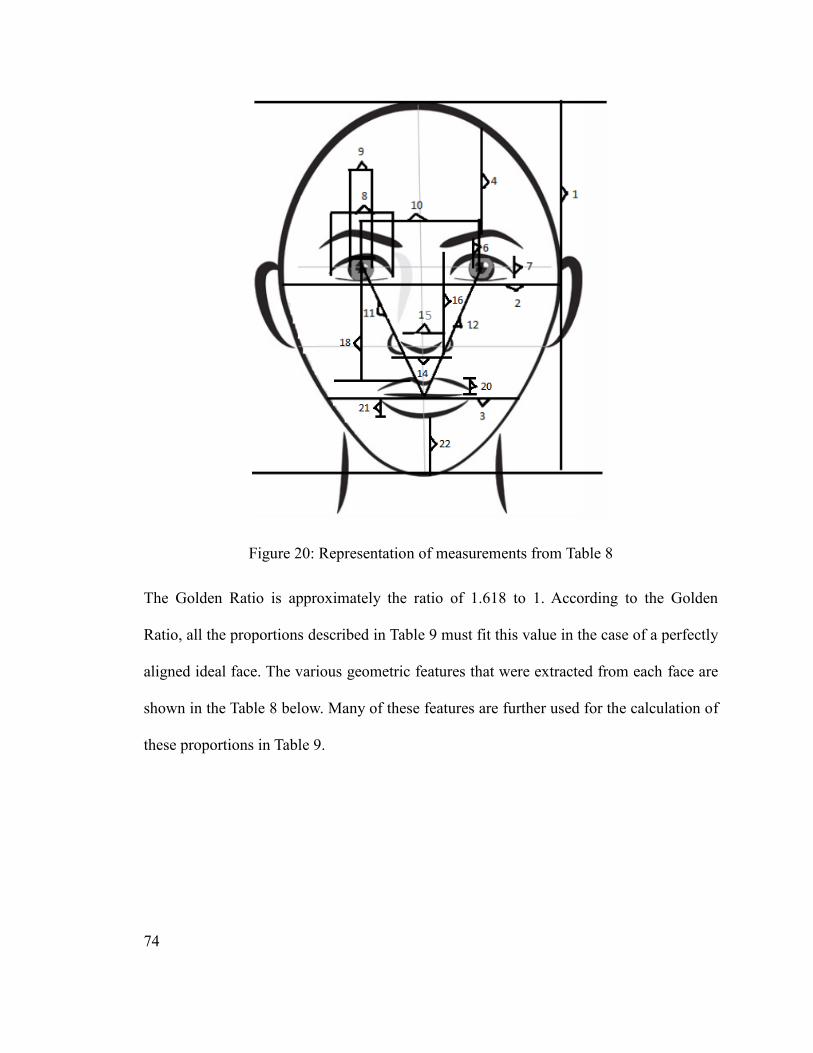
74
Figure 20: Representation of measurements from Table 8
The Golden Ratio is approximately the ratio of 1.618 to 1. According to the Golden
Ratio, all the proportions described in Table 9 must fit this value in the case of a perfectly
aligned ideal face. The various geometric features that were extracted from each face are
shown in the Table 8 below. Many of these features are further used for the calculation of
these proportions in Table 9.
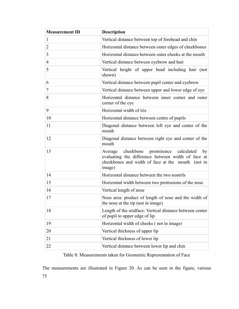
75
Measurement ID Description
1 Vertical distance between top of forehead and chin
2 Horizontal distance between outer edges of cheekbones
3 Horizontal distance between outer cheeks at the mouth
4 Vertical distance between eyebrow and hair
5 Vertical height of upper head including hair (not
shown)
6 Vertical distance between pupil center and eyebrow
7 Vertical distance between upper and lower edge of eye
8 Horizontal distance between inner corner and outer
corner of the eye
9 Horizontal width of iris
10 Horizontal distance between centre of pupils
11 Diagonal distance between left eye and center of the
mouth
12 Diagonal distance between right eye and center of the
mouth
13 Average cheekbone prominence calculated by
evaluating the difference between width of face at
cheekbones and width of face at the mouth (not in
image)
14 Horizontal distance between the two nostrils
15 Horizontal width between two protrusions of the nose
16 Vertical length of nose
17 Nose area: product of length of nose and the width of
the nose at the tip (not in image)
18 Length of the midface: Vertical distance between center
of pupil to upper edge of lip
19 Horizontal width of cheeks ( not in image)
20 Vertical thickness of upper lip
21 Vertical thickness of lower lip
22 Vertical distance between lower lip and chin
Table 8: Measurements taken for Geometric Representation of Face
The measurements are illustrated in Figure 20. As can be seen in the figure, various

76
measurements are taken which include characteristics from both the Golden Ratio
methodology and the Facial Thirds methodology.
These features represent a portion of the final feature vector that will be trained against
the training sets. However, there are several more features that are calculated according to
established ratios for facial beauty. These features are based on the Golden Ratio and
Facial Thirds methods described earlier.
The measurements taken based on the Golden Ratio theory are explained in the table
below.
Ratio ID Description
1 Vertical distance between pupils and tip of chin:
vertical distance between top of face and pupils
2 Vertical distance between face and nose:
vertical distance between nostrils and tip of the
chin
3 Vertical distance between pupils and central lip
line to vertical distance between lips and top of
the chin
4 Vertical distance between nostrils and tip of the
chin to vertical distance between pupils and
nostrils
5 Vertical distance between pupils and nostrils to
vertical distance between nostrils and lip line
6 Vertical distance between lips and top of the
chin to vertical distance between nostrils and
lip line
7 Mean of the above ratios
Table 9: List of Ratios Associated with the Golden Ratio

77
5.2.2.1 Features based on Facial Thirds Method
In addition to the above measurements, the Facial Thirds method was further utilized to
extract several meaningful features which helped to further develop an accurate
representation of the face. The Facial Thirds method states that any well proportioned
face can be divided into equal thirds by drawing lines that separate the various regions on
the face. These lines are drawn through the hairline, the eyebrows, the base of the nose
and the edge of the chin. In addition to these requirements, it is also essential that the
distance between the lips and the chin be double that of the distance between the base of
the nose and the lips.
The facial thirds divides the face in proportional regions, as can be seen in Figure 21.
78
Figure 21: Facial Thirds: The three regions on a face
The table below summarizes the various ratios are proportions that should be satisfied by
a face that is in accordance with the Facial Thirds theory.
Ratio ID
Facial Thirds Ratio Description
1 Vertical distance between top of face and
eyebrows : face length
2 Vertical distance between eyebrows and tip of
nose
3 Vertical distance between tip of nose and centre
of the line joining the upper lip
4 Vertical distance between top of nose (area
between the eyebrows) and lips to vertical
distance between lips and the tip of the chin
Table 10: List of Ratios Associated with the Facial Thirds theory
These ratios complete the geometric features component of the feature vector. Further,
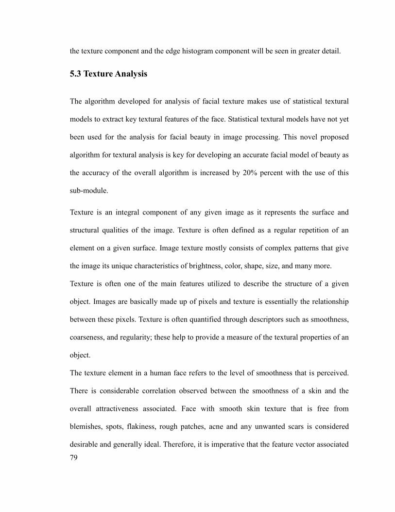
79
the texture component and the edge histogram component will be seen in greater detail.
5.3 Texture Analysis
The algorithm developed for analysis of facial texture makes use of statistical textural
models to extract key textural features of the face. Statistical textural models have not yet
been used for the analysis for facial beauty in image processing. This novel proposed
algorithm for textural analysis is key for developing an accurate facial model of beauty as
the accuracy of the overall algorithm is increased by 20% percent with the use of this
sub-module.
Texture is an integral component of any given image as it represents the surface and
structural qualities of the image. Texture is often defined as a regular repetition of an
element on a given surface. Image texture mostly consists of complex patterns that give
the image its unique characteristics of brightness, color, shape, size, and many more.
Texture is often one of the main features utilized to describe the structure of a given
object. Images are basically made up of pixels and texture is essentially the relationship
between these pixels. Texture is often quantified through descriptors such as smoothness,
coarseness, and regularity; these help to provide a measure of the textural properties of an
object.
The texture element in a human face refers to the level of smoothness that is perceived.
There is considerable correlation observed between the smoothness of a skin and the
overall attractiveness associated. Face with smooth skin texture that is free from
blemishes, spots, flakiness, rough patches, acne and any unwanted scars is considered
desirable and generally ideal. Therefore, it is imperative that the feature vector associated
80
with a given image also take into consideration the texture elements present.
Figure 22: Various textures represented
Texture is a quantitative measurement of the arrangement of intensities in a region and it
can be characterized through various methods. The methods fall into three main
categories: statistical, spectral, and structural methods [52].
Statistical methods mainly describe an attribute texture through the statistical distribution
of the intensities of the image; this is done through the analysis of distribution of gray
value intensities in a given image.
On the other hand, spectral methods base themselves on the properties of the Fourier
spectrum and essentially identify high-energy and narrow peaks. These peaks are then
used to detect the various periods present in the overall image. Furthermore, structural
techniques are associated with the arrangement of basic image components and thus
describe texture based on the spacing between lines in the image. These methods are apt
for images with textures that have many varying properties.
81
The initial approach to texture analysis included both spectral and statistic approaches.
The spectral approach was considered as it would help to represent any major patterns
occurring in the image, basically helping to establish any global patterns that were
present. The basis of the spectral approach is on three key observations. The Fourier
spectrum is ideally suited to represent global texture patterns in an image. The three main
aspects of the spectrum that are important for texture analysis are:
- Large peaks in the Fourier spectrum describe the principal direction of texture
patterns.
- Location of peaks gives the spatial pattern of textural patterns.
- After periodic elements are eliminated, the result is an image that can be further
described by statistical techniques.
The detection of textural components of an image is done by expressing the Fourier
spectrum in terms of polar coordinates. This results in two functions, S(r) and ,
where S is the Fourier spectrum function and r and are the variables of the coordinate
system.
The entire global description is obtained through the following equations [52]:
S (r )=∑θ= 1
π
Sθ(r) (7.3)
S (θ)=∑r= 1
R0
S r (θ) (7.4)
Thus, these functions essentially describe the textural aspects of the various regions of the
image under consideration. In order to further quantitatively characterize the behavior of
these functions, various descriptors are calculated. These include the highest value, the
82
mean and variance of the axial functions, and the distance between the mean and highest
value of the function. These are essentially the features that were considered for the
feature vector. However, after testing with these features, it was found that only a few
actually contributed effectively to the overall representation. Thus, these were retained
and the rest of the features were eliminated from the feature vector. The features that
were kept were those with the highest value of each function.
The main textural features utilized in this research are statistical textural features. This
specifically refers to the use of statistical moments of the image's intensity histogram to
describe texture.
A statistical moment is essentially a quantitative measure of a set of points. Assuming z to
be a random variable which represents the intensity and i = 0, 1, 2.... L-1. Here is
the corresponding histogram for these intensity levels and L is the number of distinct
intensity levels. The average intensity value, m, of z is computed by:
In addition, the nth moment of z with respect to the mean is calculated as follows:
The second moment is of great importance in texture description as it is a measure of
intensity contrast that in turn is used to describe the amount of relative smoothness
present in a particular image. The second moment is essentially the variance, which is
also represented as:
σ2(z )= μ2(z )
83
Here it is important to note that The variance is normalized to a value
between 0 and 1 as the values tend to be in a very large interval [53].
The variance is used to describe the texture through descriptors such as the value of R,
which is given below:
The value of R is 0 for areas of constant intensity. The value of R approaches 1 for areas
of rough textures. The third moment is essentially a measure of the skewness of the
histogram and a good indicator of texture properties. It is calculated with n=3, as below:
It is important to observe the uniformity of the histogram as that is often shown to be an
indicator of texture. The measure of uniformity is further then calculated using the
following:
The value of U is maximum in an image in which all intensity values are equal, meaning
it is maximally uniform. A further measurement is taken in terms of the entropy content
of an image. Entropy is a measurement of the amount of variation present in an image.
The value for an image that has constant intensities is 0. The measure of average entropy
is as follows:

84
We can illustrate this procedure with the use of an example. Let’s use the intensity
histogram below for this example.
The value for the mean for this particular image is calculated by the average of all the
intensity values as illustrated by the equation below:
This provides us with a value of 147.12. Furthermore, we must calculate the variance as
variance is an accurate measure of texture. Given a 5 X 5 region of the image for a
specific calculation, the variance is:
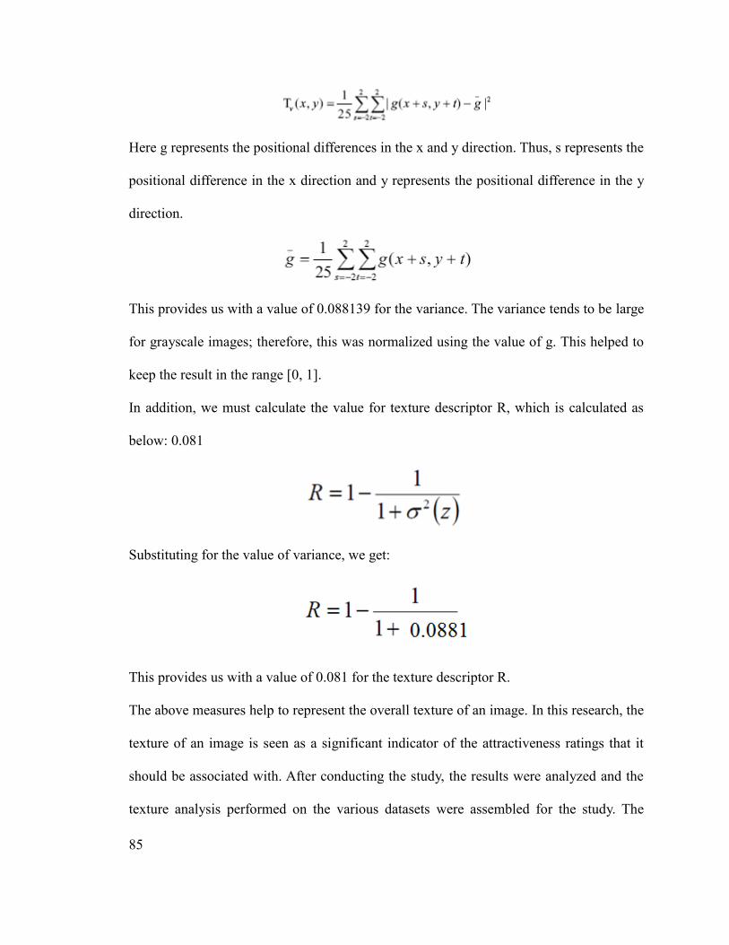
85
Here g represents the positional differences in the x and y direction. Thus, s represents the
positional difference in the x direction and y represents the positional difference in the y
direction.
This provides us with a value of 0.088139 for the variance. The variance tends to be large
for grayscale images; therefore, this was normalized using the value of g. This helped to
keep the result in the range [0, 1].
In addition, we must calculate the value for texture descriptor R, which is calculated as
below: 0.081
Substituting for the value of variance, we get:
This provides us with a value of 0.081 for the texture descriptor R.
The above measures help to represent the overall texture of an image. In this research, the
texture of an image is seen as a significant indicator of the attractiveness ratings that it
should be associated with. After conducting the study, the results were analyzed and the
texture analysis performed on the various datasets were assembled for the study. The
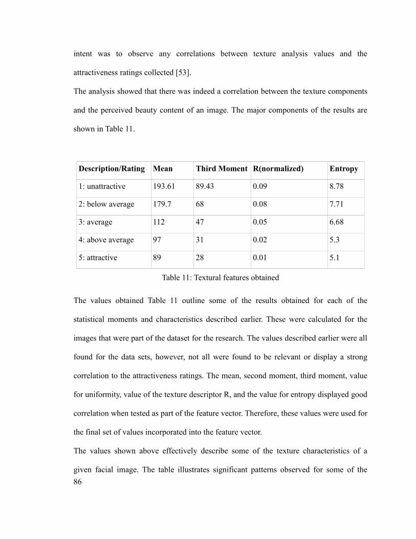
86
intent was to observe any correlations between texture analysis values and the
attractiveness ratings collected [53].
The analysis showed that there was indeed a correlation between the texture components
and the perceived beauty content of an image. The major components of the results are
shown in Table 11.
Description/Rating Mean Third Moment R(normalized) Entropy
1: unattractive 193.61 89.43 0.09 8.78
2: below average 179.7 68 0.08 7.71
3: average 112 47 0.05 6.68
4: above average 97 31 0.02 5.3
5: attractive 89 28 0.01 5.1
Table 11: Textural features obtained
The values obtained Table 11 outline some of the results obtained for each of the
statistical moments and characteristics described earlier. These were calculated for the
images that were part of the dataset for the research. The values described earlier were all
found for the data sets, however, not all were found to be relevant or display a strong
correlation to the attractiveness ratings. The mean, second moment, third moment, value
for uniformity, value of the texture descriptor R, and the value for entropy displayed good
correlation when tested as part of the feature vector. Therefore, these values were used for
the final set of values incorporated into the feature vector.
The values shown above effectively describe some of the texture characteristics of a
given facial image. The table illustrates significant patterns observed for some of the

87
texture characteristics observed.
Entropy is a measure of the amount of variability present in an image and is thus a very
important measure for the analysis of texture. Entropy helps in assessing the levels of
uniformity and variation for a given image. It was observed that an image labeled as
unattractive was associated with higher values of entropy and relatively higher values of
the texture descriptor R as well.
The texture descriptor R essentially holds the same values as the standard deviation. The
standard deviation is a key aspect to observe when taking note of the textural features of
an image. This is due to the fact that it is a measure of variability in the intensity levels of
the image. Thus, an image with a visibly smoother appearance will have a lower standard
deviation than a coarser image, as it will have lesser variability in the intensity levels.
This is a major component of the smooth appearance of many images and high intensity
values are associated with a greater occurrence of ‘smooth’ areas on a facial image. It can
be concluded that images that appeared to be possessing relatively smooth characteristics
obtained higher ratings [53].
Another interesting observation was the correlation between the values for the mean and
the attractiveness ratings obtained. Images with higher attractiveness ratings correlate
with lower values for the mean.
Figure 23 displays some images and their corresponding attractiveness ratings. The
texture feature values corresponding to these ratings can be seen in Table 11.
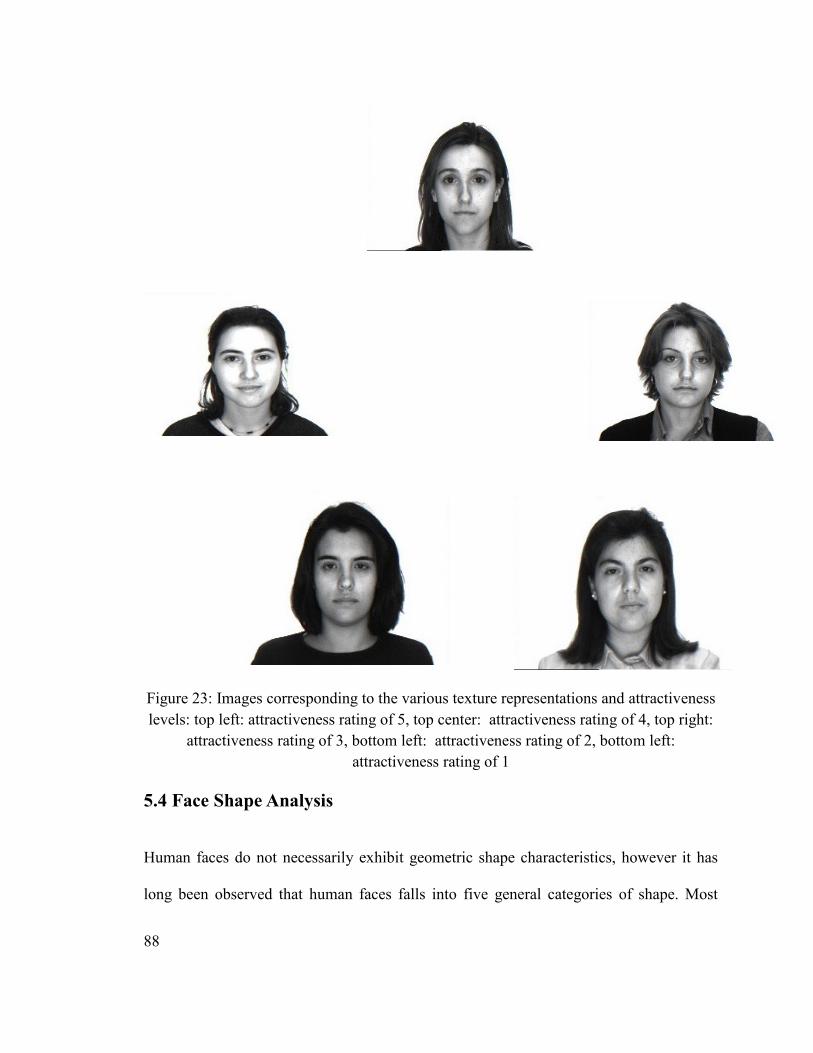
88
Figure 23: Images corresponding to the various texture representations and attractiveness
levels: top left: attractiveness rating of 5, top center: attractiveness rating of 4, top right:
attractiveness rating of 3, bottom left: attractiveness rating of 2, bottom left:
attractiveness rating of 1
5.4 Face Shape Analysis
Human faces do not necessarily exhibit geometric shape characteristics, however it has
long been observed that human faces falls into five general categories of shape. Most
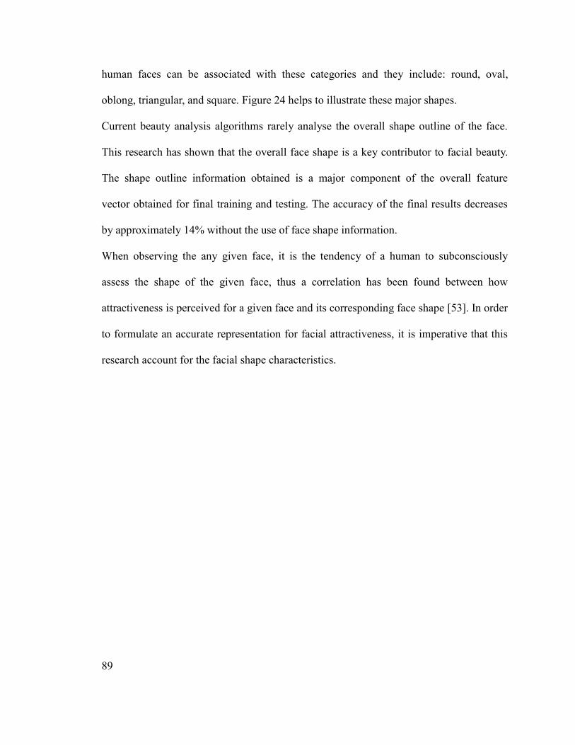
89
human faces can be associated with these categories and they include: round, oval,
oblong, triangular, and square. Figure 24 helps to illustrate these major shapes.
Current beauty analysis algorithms rarely analyse the overall shape outline of the face.
This research has shown that the overall face shape is a key contributor to facial beauty.
The shape outline information obtained is a major component of the overall feature
vector obtained for final training and testing. The accuracy of the final results decreases
by approximately 14% without the use of face shape information.
When observing the any given face, it is the tendency of a human to subconsciously
assess the shape of the given face, thus a correlation has been found between how
attractiveness is perceived for a given face and its corresponding face shape [53]. In order
to formulate an accurate representation for facial attractiveness, it is imperative that this
research account for the facial shape characteristics.

90
Figure 24: Various face shapes illustrated
The analysis was initially done with images having the resolution of 450 by 350 pixels.
Next, the resolution was increased to 800 by 720 for all the feature extraction processes
in order to obtain more accurate results. However, the feature extraction for the face
shape analysis was not producing very accurate results at this resolution; therefore the
resolution was increased to 1200 by 1024 pixels.
The algorithm developed for the analysis of facial shape is based on the concept of Sobel
operators. The algorithm improves upon the accuracy of existing Sobel operators by
working on innumerous subregions of the face in order to increase accuracy of results
obtained. Current research mainly uses Gabor wavelets for edge based feature extraction.
The use of Sobel operators for determination of facial shape characteristics is a rather
novel approach in the area of facial beauty analysis.

91
In order to apply the Sobel operator, several masks had to be applied to the various image
regions. Initially, only four masks were identified for the operation. These included the
masks for the horizontal and vertical orientations in addition to the masks for the two
diagonals. The final results were slightly improved when the mask for the non-directional
orientation was also included. The following sections help to outline the algorithm
formulated for the analysis of facial shape.
5.4.1 Edge Gradient and Face Contour
To help account for the various face shapes, the gradients of the shape outline of the face
will be examined as features to be used for training [54]. The method proposed is to build
a histogram containing the directions of the gradients of the face edges. This process can
then be divided into two sub-modules: detection of the edges and computation of the
gradients. Of greater importance is the methodology for computing edge gradient, as this
will be a significant feature for training.
The computation of edge gradient is done through Sobel operators. Then, the overall
algorithm to compute the set of gradients for the various face regions is presented. It is
important to note that the overall face image is divided into small subregions in order to
isolate the regions containing the outline of the face shape [55].
Thus, given an image it is divided into subregions of equal size, as can be seen in Figure
25 below. In the case of this image, there is a mask dividing the image into smaller
squares that will be processed individually.

92
Figure 25: Various steps of dividing the image into subregions
Only the regions along the face contour are then sampled for gradient information. This is
a relatively new approach to face beauty analysis as the role of the overall holistic face
shape has not been examined in detail before. The edges in the regions along the face
shape outline are key aspects for the representation of any face. In order to define the
edges of the face, the landmarks detected from the Active Shape Models are used. Thus,
the regions of the face containing the points outlining the face are analyzed for gradient
information, as seen in Figure 26.
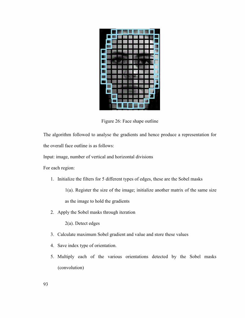
93
Figure 26: Face shape outline
The algorithm followed to analyse the gradients and hence produce a representation for
the overall face outline is as follows:
Input: image, number of vertical and horizontal divisions
For each region:
1. Initialize the filters for 5 different types of edges, these are the Sobel masks
1(a). Register the size of the image; initialize another matrix of the same size
as the image to hold the gradients
2. Apply the Sobel masks through iteration
2(a). Detect edges
3. Calculate maximum Sobel gradient and value and store these values
4. Save index type of orientation.
5. Multiply each of the various orientations detected by the Sobel masks
(convolution)
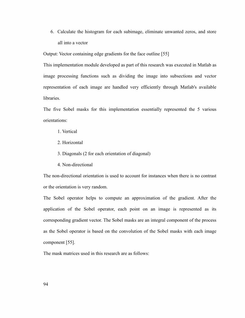
94
6. Calculate the histogram for each subimage, eliminate unwanted zeros, and store
all into a vector
Output: Vector containing edge gradients for the face outline [55]
This implementation module developed as part of this research was executed in Matlab as
image processing functions such as dividing the image into subsections and vector
representation of each image are handled very efficiently through Matlab's available
libraries.
The five Sobel masks for this implementation essentially represented the 5 various
orientations:
1. Vertical
2. Horizontal
3. Diagonals (2 for each orientation of diagonal)
4. Non-directional
The non-directional orientation is used to account for instances when there is no contrast
or the orientation is very random.
The Sobel operator helps to compute an approximation of the gradient. After the
application of the Sobel operator, each point on an image is represented as its
corresponding gradient vector. The Sobel masks are an integral component of the process
as the Sobel operator is based on the convolution of the Sobel masks with each image
component [55].
The mask matrices used in this research are as follows:
95
-1 -2 -1
0 0 0
+1 +2 +1
-1 0 +1
-2 0 +2
-1 0 +1
+2 +2 -1
+2 -1 -1
-1 -1 -1
-1 +2 +2
-1 -1 +2
1 -1 -1
-1 0 +1
0 0 0
1 0 -1
Figure 27: Masks for the various orientations: (from left) vertical, horizontal, diagonal1,
diagonal2, non-directional)
The convolution of each image subregion with each of these masks produces another
matrix equivalent in size with the original image subregion. Convolution is essentially a
mathematical operation on two functions which outputs the area overlap between the two
functions as a relation of the amount that one of the functions is translated. The
convolution process gives the derivatives for the various orientations. The resulting
gradient approximations are then combined to give the overall gradient magnitude and
direction.
The Sobel operator represents the gradient in a sufficiently accurate quality to be used in
this application. Nevertheless, it has several drawbacks as well, which include the fact
that intensity values in a very small region are sampled in each iteration, increasing the
number of iterations needed for an accurate value [55].
96
Chapter 6 Experimental Results
Facial beauty is one of the few characteristics that humans often derive happiness from.
Naturally, it has long been an area of considerable research in image processing. Having
various applications ranging from surgery and facial reconstruction to cosmetics, facial
beauty analysis can be used as a stand-alone module in addition to being integrated into
larger image processing systems.
This chapter discusses the results obtained from the implementation. The extraction of
features is proposed through the identification of landmarks using an algorithm based on
the Active Shape Model algorithm. The landmarks are then used for the extraction of
geometric, textural, and shape features related to a given face. The sub modules for
extracting accurate geometric, textural and shape features are all based on algorithms
developed and tested as part of this research. The ratios extracted from the landmarked
geometric features were extracted based on an algorithm developed that calculated the
distances among the various features. The textural features were extracted based on
procedures and modules developed to extract textural information from each image from
the database. The shape features were extracted using a Matlab module developed for
efficient utilization of the Sobel operator which was an integral part of the shape
extraction algorithm.
The algorithms pertaining to the various sub-modules developed have been previously
outlined in Chapter 5. The final system developed is outlined below in Figure 28, which
shows the significant components and steps followed to establish the system.

97
Figure 28: Block Diagram of Beauty Analysis System

98
Various feature vectors were tested before converging to a vector which produced
consistent results. However, in order to plot landmarks and extract these features, the
image size needed to be optimum. The results varied according to several key factors,
which included the image size and resolution, accuracy of landmark selection, the
features selected, and the size of training samples. The final result converged to an
accuracy of 85.66 percent.
6.1 Feature Classification
Previous sections of this chapter discuss the various features that are part of the main
feature vector used for training. This section will help to outline the results obtained by
using Support Vector Machines for the classification of images into the various categories
of attractiveness. As mentioned earlier, the five main classes to which an image can be
assigned are as follows:
1. Unattractive
2. Below average
3. Average
4. Above average
5. Attractive
6.1.1 Support Vector Machines
Features are necessary to accurately represent a given face as they can quantify the
essence of facial beauty. In order to determine how accurate the representation is, the
feature vector must be tested through a learning system, which will attempt to learn the

99
structure of a set of data through training. The learning system is the decision module
which will eventually provide the final output.
There are two main types of learning models in machine learning:
- supervised learning
- unsupervised learning
Supervised learning infers patterns from a set of labeled training data, which is made up
of a set of training samples. Thus, each piece of training data consists of an input value
and its corresponding output value. The supervised learning algorithm then analyzes the
training data and produces a function as a result. This function is then used to predict the
outputs of further new input data.
Unsupervised learning, on the other hand, attempts to find patterns in unlabeled data and
thus there is no error checking mechanism for the evaluation of a potential solution.
The learning methodology utilized in this research is supervised learning, through
Support Vector Machines. Support vector machines (SVMs) are supervised learning
models that analyze and record patterns which are then used to classify data. A support
vector machine does this by building the optimal hyperplane for linearly separable data.
The support vectors are the data points that lie closest to the decision surface and have the
greatest effect on the ideal location of the decision surface [59].
The best hyperplane for separation of the data is one that has the largest distance to the
nearest training data point of a given class, this is known as the functional margin. Larger
functional margins usually lead to lowering the generalization error for the classifier. The
generalization error essentially measures the ability for a learning machine to generalize
to unseen data. This is illustrated in the figure below; as can be seen, three possible
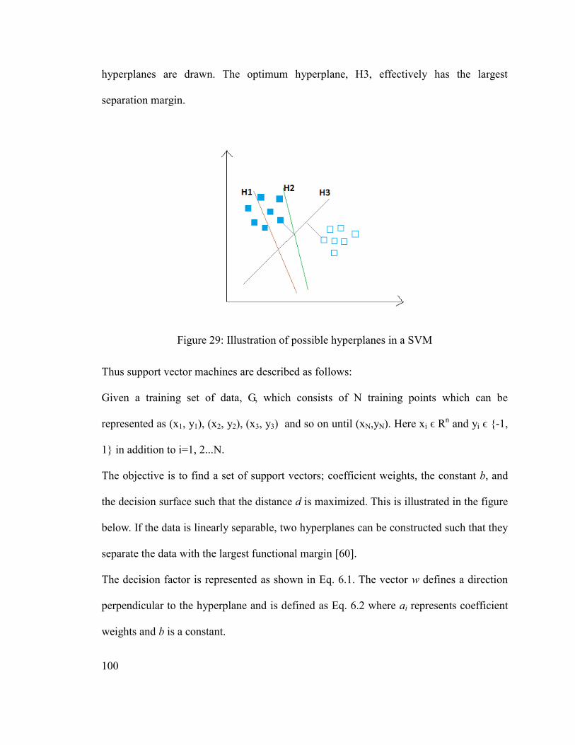
100
hyperplanes are drawn. The optimum hyperplane, H3, effectively has the largest
separation margin.
Figure 29: Illustration of possible hyperplanes in a SVM
Thus support vector machines are described as follows:
Given a training set of data, G, which consists of N training points which can be
represented as (x1, y1), (x2, y2), (x3, y3) and so on until (xN,yN). Here xi ϵ Rn and yi ϵ {-1,
1} in addition to i=1, 2...N.
The objective is to find a set of support vectors; coefficient weights, the constant b, and
the decision surface such that the distance d is maximized. This is illustrated in the figure
below. If the data is linearly separable, two hyperplanes can be constructed such that they
separate the data with the largest functional margin [60].
The decision factor is represented as shown in Eq. 6.1. The vector w defines a direction
perpendicular to the hyperplane and is defined as Eq. 6.2 where ai represents coefficient
weights and b is a constant.

101
wT
x+ b= 0 (6.1)
W =∑i= 1
N
ai yi xi
(6.2)
Figure 30: Construction of two main hyperplanes
6.1.1.1 Nonlinear Classification
In the case that the training data, Φ, is not linearly separable, the nonlinearly separable
data is mapped into a higher dimensional Euclidean space where data can be linearly
separated. This is done through the use of a kernel function, K, where K is defined by
Eq. 6.3.
Figure 31 illustrates the mapping of the data into the higher dimension.
K ( xi , x j)=Φ(xi) ,Φ( x j) 6.3
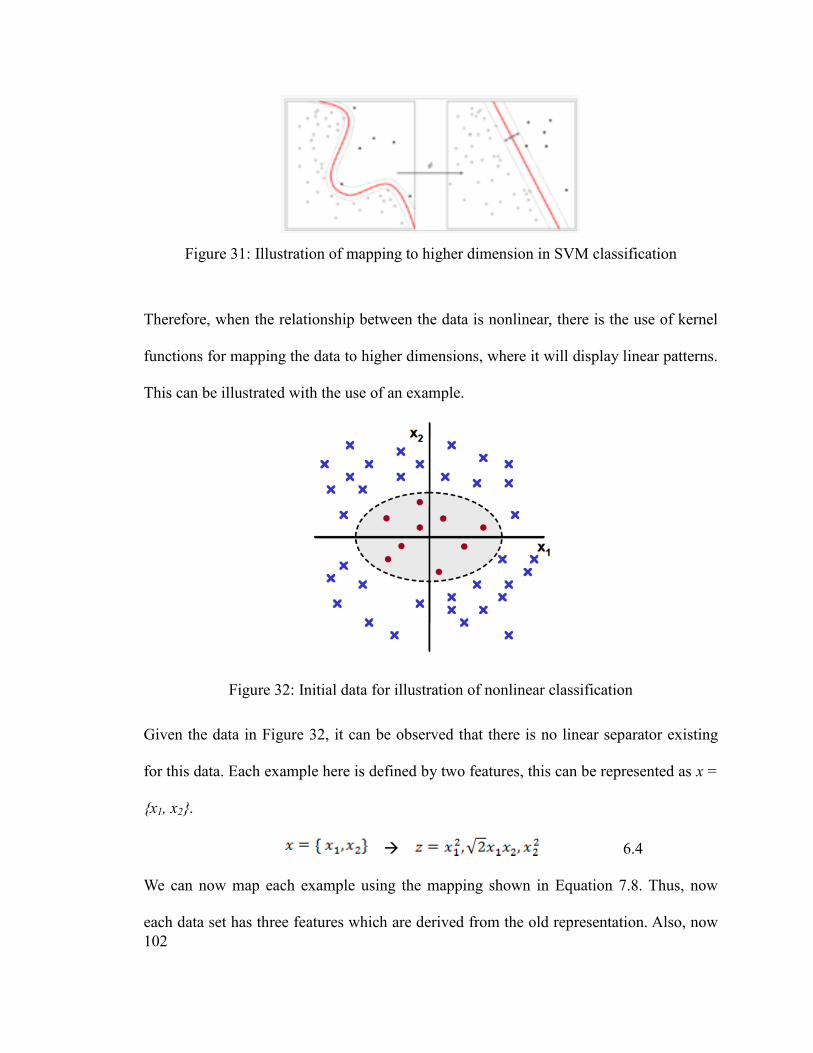
102
Figure 31: Illustration of mapping to higher dimension in SVM classification
Therefore, when the relationship between the data is nonlinear, there is the use of kernel
functions for mapping the data to higher dimensions, where it will display linear patterns.
This can be illustrated with the use of an example.
Figure 32: Initial data for illustration of nonlinear classification
Given the data in Figure 32, it can be observed that there is no linear separator existing
for this data. Each example here is defined by two features, this can be represented as x =
{x1, x2}.
6.4
We can now map each example using the mapping shown in Equation 7.8. Thus, now
each data set has three features which are derived from the old representation. Also, now
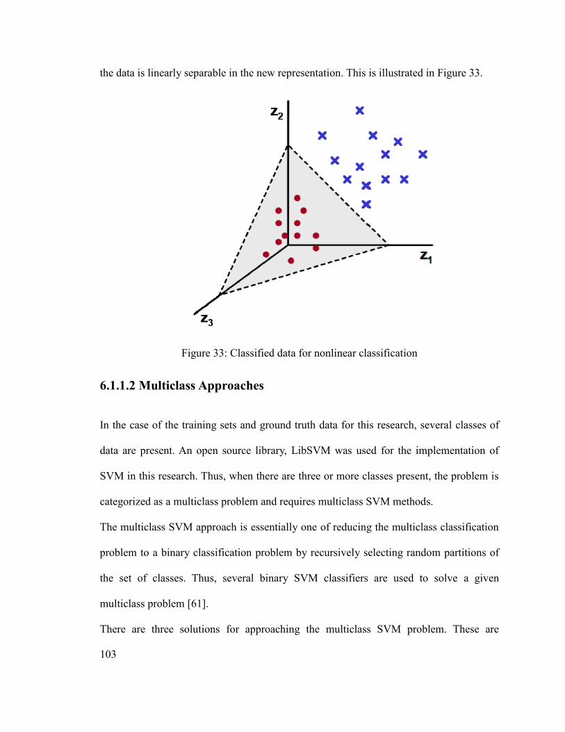
103
the data is linearly separable in the new representation. This is illustrated in Figure 33.
Figure 33: Classified data for nonlinear classification
6.1.1.2 Multiclass Approaches
In the case of the training sets and ground truth data for this research, several classes of
data are present. An open source library, LibSVM was used for the implementation of
SVM in this research. Thus, when there are three or more classes present, the problem is
categorized as a multiclass problem and requires multiclass SVM methods.
The multiclass SVM approach is essentially one of reducing the multiclass classification
problem to a binary classification problem by recursively selecting random partitions of
the set of classes. Thus, several binary SVM classifiers are used to solve a given
multiclass problem [61].
There are three solutions for approaching the multiclass SVM problem. These are

104
described as follows:
Ranking SVMs for Multiclass Problems: In this methodology, one SVM decision
function is used for the classification of all classes.
One-Versus-All Method: One binary SVM is constructed to separate members of
a given class from members of other classes.
One-Versus-One: One binary SVM is constructed for pairs of classes in order to
separate members of a given class from members of other classes.
The methodology selected for use in this research is the One-Versus-One approach, as the
performance was significantly better for this data set and training time was shorter as
well. The One-Versus-One approach is based on the max-wins voting strategy, in which
the result is obtained by majority vote of all classifiers. In this strategy, every classifier
chooses one of two classes to assign, then the vote for the class to which the assignment
is made is increased by one. The class with the most votes in the final stage determines
the final classification. Therefore, the class that is chosen is the one with votes from the
maximal number of pairs of SVMs.
An illustration of the one-versus-one approach for multiclass SVM with three classes is
shown in Figure 34. This figure shows the various pair-wise decision boundaries that are
constructed for each pair of classes.
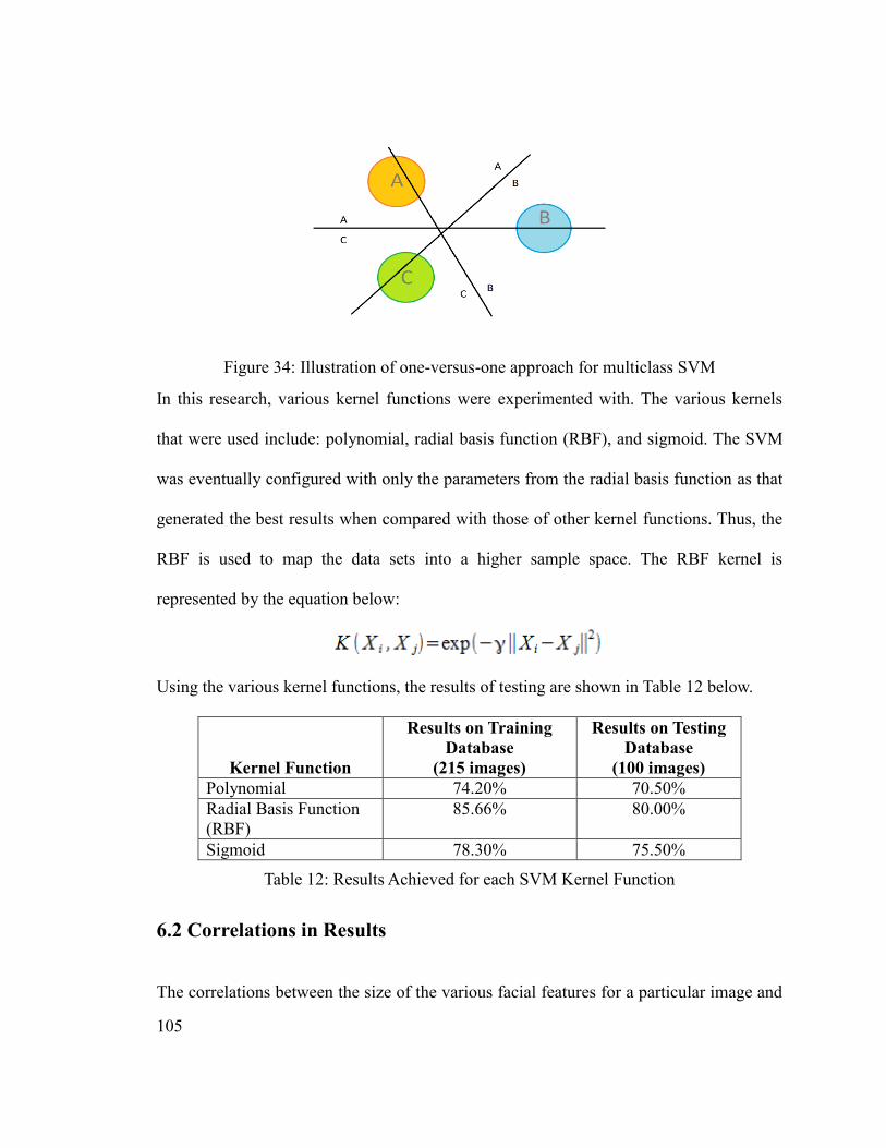
105
Figure 34: Illustration of one-versus-one approach for multiclass SVM
In this research, various kernel functions were experimented with. The various kernels
that were used include: polynomial, radial basis function (RBF), and sigmoid. The SVM
was eventually configured with only the parameters from the radial basis function as that
generated the best results when compared with those of other kernel functions. Thus, the
RBF is used to map the data sets into a higher sample space. The RBF kernel is
represented by the equation below:
Using the various kernel functions, the results of testing are shown in Table 12 below.
Kernel Function
Results on Training
Database
(215 images)
Results on Testing
Database
(100 images)
Polynomial 74.20% 70.50%
Radial Basis Function
(RBF)
85.66% 80.00%
Sigmoid 78.30% 75.50%
Table 12: Results Achieved for each SVM Kernel Function
6.2 Correlations in Results
The correlations between the size of the various facial features for a particular image and
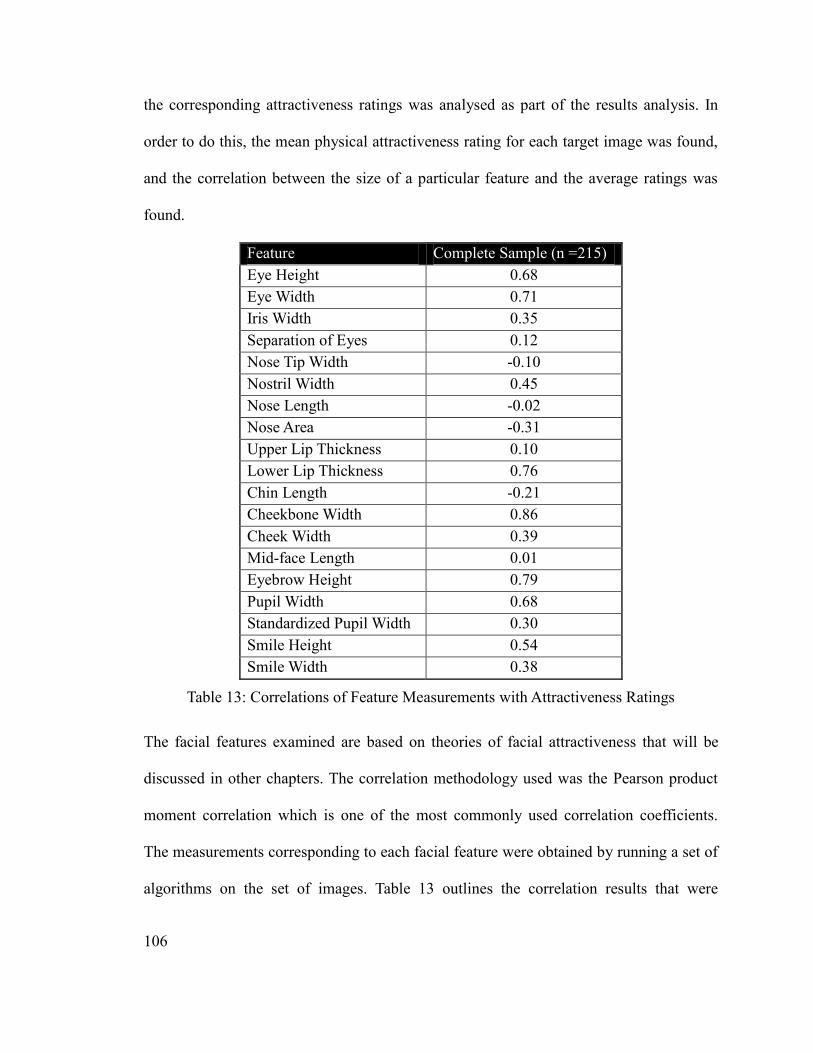
106
the corresponding attractiveness ratings was analysed as part of the results analysis. In
order to do this, the mean physical attractiveness rating for each target image was found,
and the correlation between the size of a particular feature and the average ratings was
found.
Feature Complete Sample (n =215)
Eye Height 0.68
Eye Width 0.71
Iris Width 0.35
Separation of Eyes 0.12
Nose Tip Width -0.10
Nostril Width 0.45
Nose Length -0.02
Nose Area -0.31
Upper Lip Thickness 0.10
Lower Lip Thickness 0.76
Chin Length -0.21
Cheekbone Width 0.86
Cheek Width 0.39
Mid-face Length 0.01
Eyebrow Height 0.79
Pupil Width 0.68
Standardized Pupil Width 0.30
Smile Height 0.54
Smile Width 0.38
Table 13: Correlations of Feature Measurements with Attractiveness Ratings
The facial features examined are based on theories of facial attractiveness that will be
discussed in other chapters. The correlation methodology used was the Pearson product
moment correlation which is one of the most commonly used correlation coefficients.
The measurements corresponding to each facial feature were obtained by running a set of
algorithms on the set of images. Table 13 outlines the correlation results that were
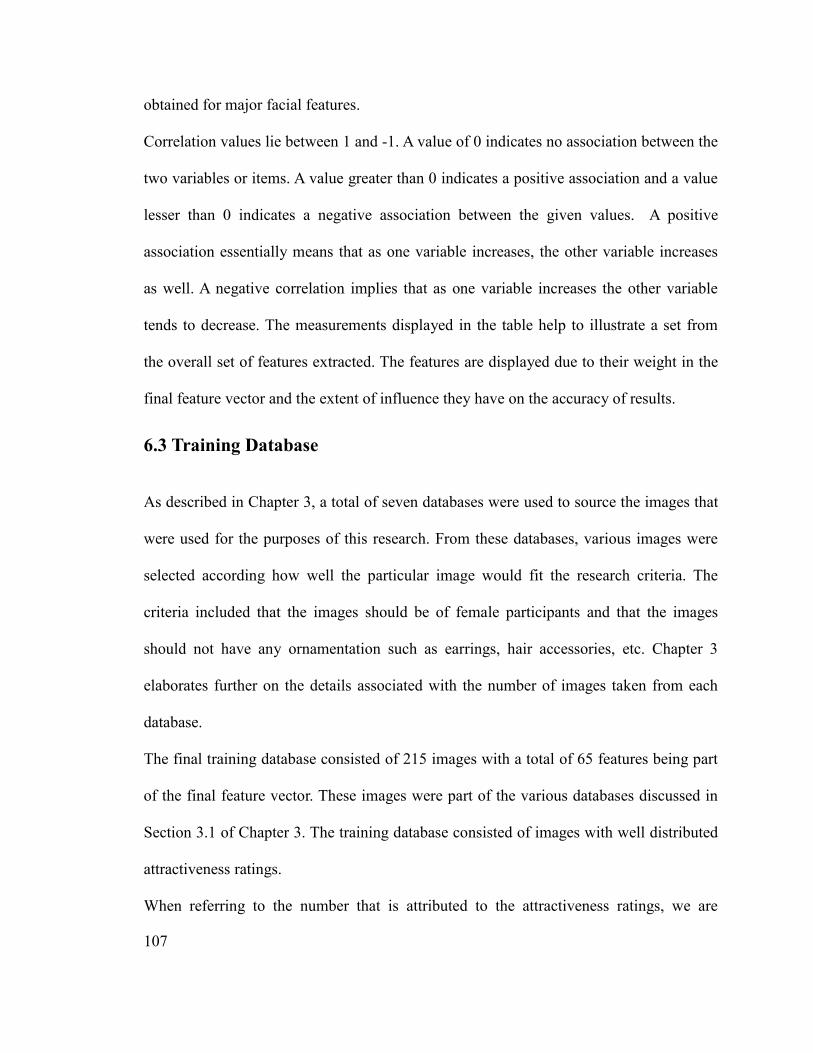
107
obtained for major facial features.
Correlation values lie between 1 and -1. A value of 0 indicates no association between the
two variables or items. A value greater than 0 indicates a positive association and a value
lesser than 0 indicates a negative association between the given values. A positive
association essentially means that as one variable increases, the other variable increases
as well. A negative correlation implies that as one variable increases the other variable
tends to decrease. The measurements displayed in the table help to illustrate a set from
the overall set of features extracted. The features are displayed due to their weight in the
final feature vector and the extent of influence they have on the accuracy of results.
6.3 Training Database
As described in Chapter 3, a total of seven databases were used to source the images that
were used for the purposes of this research. From these databases, various images were
selected according how well the particular image would fit the research criteria. The
criteria included that the images should be of female participants and that the images
should not have any ornamentation such as earrings, hair accessories, etc. Chapter 3
elaborates further on the details associated with the number of images taken from each
database.
The final training database consisted of 215 images with a total of 65 features being part
of the final feature vector. These images were part of the various databases discussed in
Section 3.1 of Chapter 3. The training database consisted of images with well distributed
attractiveness ratings.
When referring to the number that is attributed to the attractiveness ratings, we are

108
referring to the scale that was used for the attractiveness ratings survey. The survey
utilized a scale which ranged from 1 to 5, with 1 corresponding to a rating of
“unattractive”, 2 corresponding to a rating of “below average”, 3 corresponding to a
rating of “average”, 4 corresponding to a rating of “above average” and 5 corresponding
to a rating of “attractive”, which corresponds to the attractiveness of the individual in the
image being described as “average”.
Among the images used for training, 68 of the images had been assigned an average
attractiveness rating of 3. A total of 17 images with the attractiveness rating of 1 were
further selected and a total of 50 images with the rating of 2 were selected. There were
also 58 images with a rating of 4, and 22 images with an average attractiveness rating of
5. The distribution and corresponding numbers are outlined in Figure 35. The
attractiveness ratings from the survey conducted previously were used as the ground truth
data for the database.

109
Figure 35: Number of Images in Training Database Corresponding to each Rating
6.4 Testing Database
A total of 100 images were used for the testing process. The feature vector is extracted for
the given set of images that were part of the testing database. The vector is then classified
into one of the five attractiveness classes. In addition, Figure 36 summarizes the number
of images corresponding to each attractiveness rating.
During the testing phase, several variations of the feature vector were experimented with
in order to result in a vector with the optimum features for representing the human face
accurately. In the case of geometric features, there was considerable difficulty in finding
the right mix of features for resulting in the highest accuracy. There were a great number
of combinations and going through all the combinations manually was painstaking,

110
therefore a quick method was determined to permute through the various combinations of
geometric features from each set.
The next set of features included the textural features, which were made up of three main
groups. This included spectral, statistical and structural textural features. It was important
to isolate the category of features that best applied for the representation of the human
face. Through several tests and experimentation, it was determined that the statistical
textural features were best suited for the purposes of this research.
The final set of features used included features for edge orientation information; this set
of features was used mainly to represent the overall face shape and outline. This was a set
of features of considerable importance as the overall face shape is known to be a deciding
factor when it comes to measuring attractiveness levels in a given human face. However,
there was an error that was occurring from the measurement taken from the area near the
chin. The features being extracted from the chin and the nearby region were not being
accurately represented. Therefore, it was decided that this region will be broken down
into more parts than what was applied to the rest of the face. This means to say that
although the outline of the face was being broken down into small squares for the
extraction of edge information, the area near the chin would have the squares broken
down further into small component squares. This iterative approach helped to gain more
accurate face shape and edge outline information.

111
Figure 36: Number of Images in Testing Database Corresponding to each Rating
6.5 Values Utilized
The experimental results were obtained with the variation of values chosen for C and γ.
These approximate values were obtained through cross validation and a parse grid search,
in which the available data are split into a given number of subsets. The cross validation
error is then computed for various values for C and γ. Finally, the C and γ with the lowest
cross validation error is chosen for use on the training data set.
After obtaining an approximation for values of C and γ, adjustments were made to the
values in order to improve the performance results. The values of C and γ that were found
to have the highest classification rates were C=0.0625 and γ = 0.00390625.
Shown in Figure 37 are some images that were wrongly classified during the testing
process. It could be hypothesized that the reason why these images were incorrectly
classified was because the face had slight amounts of hair covering the outline of the
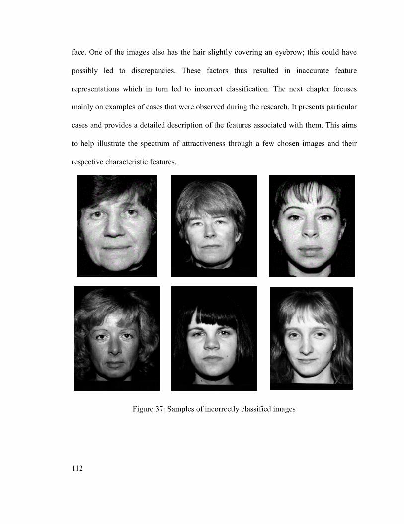
112
face. One of the images also has the hair slightly covering an eyebrow; this could have
possibly led to discrepancies. These factors thus resulted in inaccurate feature
representations which in turn led to incorrect classification. The next chapter focuses
mainly on examples of cases that were observed during the research. It presents particular
cases and provides a detailed description of the features associated with them. This aims
to help illustrate the spectrum of attractiveness through a few chosen images and their
respective characteristic features.
Figure 37: Samples of incorrectly classified images

113
Chapter 7 Illustrative Examples
This thesis aims to present an automatic system for the analysis of female facial beauty.
The efforts have been concentrated around developing an accurate representation of the
aesthetic aspects of the human face. This representation was then utilized for the purposes
of analyzing each image. The analysis aided in the evaluation of an attractiveness rating
for the given image. The attractiveness spectrum ranged from “unattractive” to
“attractive”, with ratings of 1 and 5 respectively. All images were normalized prior to
feature extraction and testing.
To help illustrate the values associated with each attractiveness level, a few examples are
presented below. For each example, a detailed description is given of the various features
that were extracted for all the various aspects which include the geometric aspects, the
textural aspects, and the facial shape aspects. For each feature group, the actual results
obtained are given in detail. This thus aims to present a subset of the actual set of results
finally obtained. The values included in the table are representative of the final feature
vector used for training, the features shown below were particularly chosen because they
had great weight in the final feature vector and contributed greatly to the accuracy while
testing.

114
7.1 Attractiveness Level 1
Figure 38: Image with attractiveness rating of 1
7.1.1 Geometric Features
Table 14 shows the values obtained for the geometric features for the given image in
Figure 38. This image received an overall attractiveness rating of 1. The geometric
representation takes into consideration various theories of facial geometry, which include
the Facial Thirds method and the Golden Ratio. Applying these theories helps create an
accurate representation of the human face. The table below shows the values obtained for
several of the ratios that were calculated for the final feature vector. For each image, the

115
landmarks were initially detected directly on the image itself, and then the map of labeled
points was scaled to a coordinate system. Finally, an automatic computer application was
programmed to compute each of the measurements associated with the geometric feature
vector.
Measurement ID Description
Value for
Measurement(cm)
1 Vertical distance between top of
forehead and chin
4.22
2 Horizontal distance between outer
edges of cheekbones
3.73
3 Horizontal distance between outer
cheeks at the mouth
2.14
4 Vertical distance between eyebrow and
hair
1.45
5 Vertical length of upper head including
hair (not shown)
5.79
6 Vertical distance between pupil center
and eyebrow
1.21
7 Vertical distance between upper and
lower edge of eye
0.59
8 Horizontal distance between inner
corner and outer corner of the eye
1.78
9 Horizontal width of iris 0.39
10 Horizontal distance between centre of
pupils
3.84
11 Diagonal distance between left eye and
center of the mouth
3.11
12 Diagonal distance between right eye
and center of the mouth
3.1
Table 14: Values of sample geometric measurements
7.1.2 Textural Features
Table 15 displays a sample of the textural results that was obtained for the image shown
in Figure 38. These values shown are typical ones obtained for many other images in the
same attractiveness category as this image. The values of the third moment, R, and
116
Entropy are the highest in comparison with the images that received a higher
attractiveness rating; this is mostly due to the presence of greater levels of variation in the
image.
Mean Third Moment R(normalized) Entropy
197.34 84.14 0.08 8.18
Table 15: Values of sample textural features
7.1.3 Facial Shape Features
The facial shape obtained for this particular image was square. This overall face shape
was determined through the face shape analysis done through the Sobel filters and masks.
In the scope of this research, the square face shape was observed to be less likely to be
associated with a very high attractiveness rating.

117
7.2 Attractiveness Level 2
Figure 39: Image with attractiveness rating of 2
7.2.1 Geometric Features
Table 16 shows the values obtained for the geometric features for the given image in
Figure 39. This image received an overall attractiveness rating of 2.

118
Measurement ID Description
Value for
Measurement(cm)
1 Vertical distance between top of
forehead and chin
5.17
2 Horizontal distance between outer
edges of cheekbones
3.69
3 Horizontal distance between outer
cheeks at the mouth
2.25
4 Vertical distance between eyebrow and
hair
1.57
5 Vertical length of upper head including
hair (not shown)
6.1
6 Vertical distance between pupil center
and eyebrow
1.17
7 Vertical distance between upper and
lower edge of eye
0.61
8 Horizontal distance between inner
corner and outer corner of the eye
1.71
9 Horizontal width of iris 0.43
10 Horizontal distance between centre of
pupils
3.89
11 Diagonal distance between left eye and
center of the mouth
3.15
12 Diagonal distance between right eye
and center of the mouth
3.13
Table 16: Values of sample geometric measurements
7.2.2 Textural Features
Table 17 displays a sample of the textural results that was obtained for the image shown
in Figure 39. These are typical values obtained for many other images in the same
attractiveness category as this image. The values of the third moment, R, and Entropy are
the second highest in comparison with the images that received a higher attractiveness
rating. This is mostly due to the presence of greater levels of variation in the image.
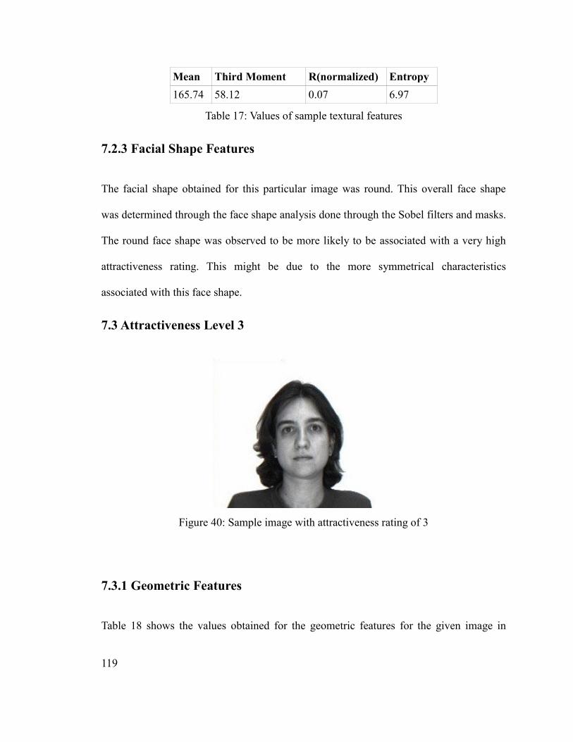
119
Mean Third Moment R(normalized) Entropy
165.74 58.12 0.07 6.97
Table 17: Values of sample textural features
7.2.3 Facial Shape Features
The facial shape obtained for this particular image was round. This overall face shape
was determined through the face shape analysis done through the Sobel filters and masks.
The round face shape was observed to be more likely to be associated with a very high
attractiveness rating. This might be due to the more symmetrical characteristics
associated with this face shape.
7.3 Attractiveness Level 3
Figure 40: Sample image with attractiveness rating of 3
7.3.1 Geometric Features
Table 18 shows the values obtained for the geometric features for the given image in
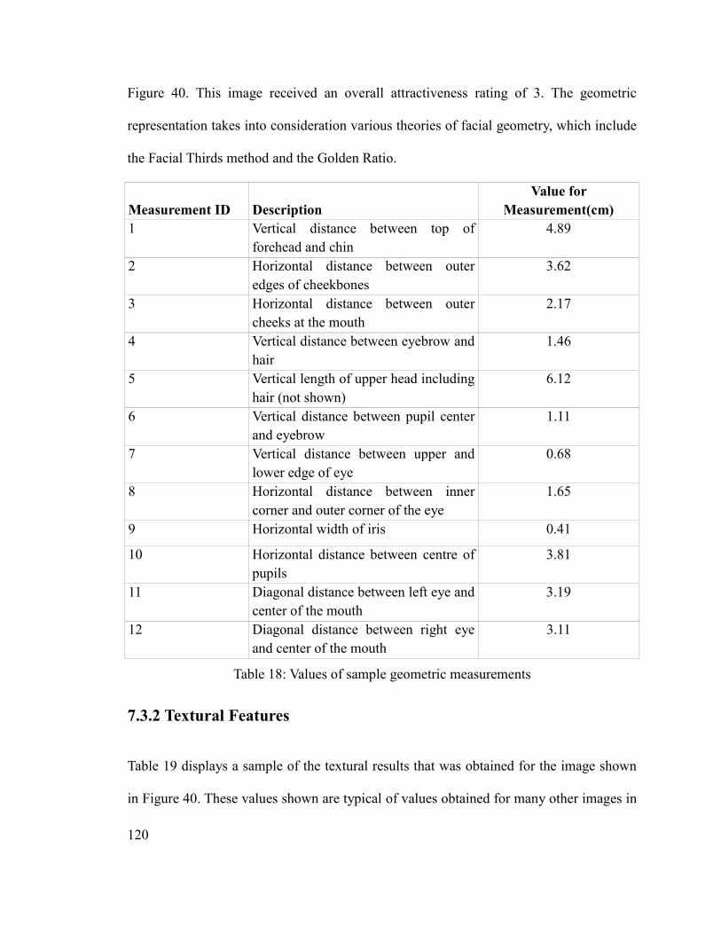
120
Figure 40. This image received an overall attractiveness rating of 3. The geometric
representation takes into consideration various theories of facial geometry, which include
the Facial Thirds method and the Golden Ratio.
Measurement ID Description
Value for
Measurement(cm)
1 Vertical distance between top of
forehead and chin
4.89
2 Horizontal distance between outer
edges of cheekbones
3.62
3 Horizontal distance between outer
cheeks at the mouth
2.17
4 Vertical distance between eyebrow and
hair
1.46
5 Vertical length of upper head including
hair (not shown)
6.12
6 Vertical distance between pupil center
and eyebrow
1.11
7 Vertical distance between upper and
lower edge of eye
0.68
8 Horizontal distance between inner
corner and outer corner of the eye
1.65
9 Horizontal width of iris 0.41
10 Horizontal distance between centre of
pupils
3.81
11 Diagonal distance between left eye and
center of the mouth
3.19
12 Diagonal distance between right eye
and center of the mouth
3.11
Table 18: Values of sample geometric measurements
7.3.2 Textural Features
Table 19 displays a sample of the textural results that was obtained for the image shown
in Figure 40. These values shown are typical of values obtained for many other images in
121
the same attractiveness category as this image. The values of the third moment, R, and
Entropy are the generally high in comparison with the images that received a higher
attractiveness rating. This is mostly due to the presence of greater levels of variation in
the image.
Mean Third Moment R(normalized) Entropy
121.14 50.73 0.04 6.51
Table 19: Values of sample textural features
7.3.3 Facial Shape Features
The facial shape obtained for this particular image was round. This overall face shape
was determined through the face shape analysis done through the Sobel filters and masks.
The round face shape was observed to be more likely to be associated with a very high
attractiveness rating. This might be due to the more symmetrical characteristics
associated with this face shape.
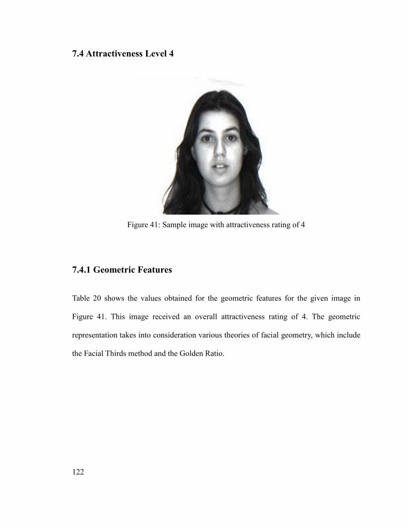
122
7.4 Attractiveness Level 4
Figure 41: Sample image with attractiveness rating of 4
7.4.1 Geometric Features
Table 20 shows the values obtained for the geometric features for the given image in
Figure 41. This image received an overall attractiveness rating of 4. The geometric
representation takes into consideration various theories of facial geometry, which include
the Facial Thirds method and the Golden Ratio.

123
Measurement ID Description
Value for
Measurement(cm)
1 Vertical distance between top of
forehead and chin
5.12
2 Horizontal distance between outer
edges of cheekbones
3.86
3 Horizontal distance between outer
cheeks at the mouth
2.25
4 Vertical distance between eyebrow and
hair
1.53
5 Vertical length of upper head including
hair (not shown)
6.19
6 Vertical distance between pupil center
and eyebrow
1.16
7 Vertical distance between upper and
lower edge of eye
0.73
8 Horizontal distance between inner
corner and outer corner of the eye
1.82
9 Horizontal width of iris 0.57
10 Horizontal distance between centre of
pupils
3.86
11 Diagonal distance between left eye and
center of the mouth
3.21
12 Diagonal distance between right eye
and center of the mouth
3.13
Table 20: Values of sample geometric measurements
7.4.2 Textural Features
Table 21 displays a sample of the textural results that was obtained for the image shown
in Figure 41. These values shown are typical of values obtained for many other images in
the same attractiveness category as this image. The values of the third moment, R, and
Entropy are the generally lower in comparison with the images that received higher
attractiveness ratings. This is mostly due to the presence of lower levels of variation in
the image.

124
Mean Third Moment R(normalized) Entropy
109.15 34.62 0.03 5.35
Table 21: Values of sample textural features
The high attractiveness rating could be associated with the ideal textural feature values,
this could be explained by the fact that theoretically faces with smoother textures are
often found to be more attractive.
7.4.3 Facial Shape Features
The facial shape obtained for this particular image was oval. This overall face shape was
determined through the face shape analysis done through the Sobel filters and masks. The
oval face shape was observed to be most likely to be associated with a very high
attractiveness rating. This might be due to the symmetrical characteristics associated with
this face shape.
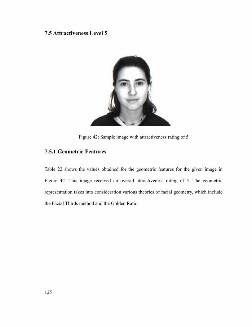
125
7.5 Attractiveness Level 5
Figure 42: Sample image with attractiveness rating of 5
7.5.1 Geometric Features
Table 22 shows the values obtained for the geometric features for the given image in
Figure 42. This image received an overall attractiveness rating of 5. The geometric
representation takes into consideration various theories of facial geometry, which include
the Facial Thirds method and the Golden Ratio.

126
Measurement ID Description
Value for
Measurement(cm)
1 Vertical distance between top of
forehead and chin
5.25
2 Horizontal distance between outer
edges of cheekbones
3.83
3 Horizontal distance between outer
cheeks at the mouth
2.26
4 Vertical distance between eyebrow and
hair
1.51
5 Vertical length of upper head including
hair (not shown)
5.98
6 Vertical distance between pupil center
and eyebrow
1.24
7 Vertical distance between upper and
lower edge of eye
0.59
8 Horizontal distance between inner
corner and outer corner of the eye
1.61
9 Horizontal width of iris 0.52
10 Horizontal distance between centre of
pupils
3.62
11 Diagonal distance between left eye and
center of the mouth
3.35
12 Diagonal distance between right eye
and center of the mouth
3.11
Table 22: Values of sample geometric measurements
7.5.2 Textural Features
Table 23 displays a sample of the textural results that was obtained for the image shown
in Figure 42. These values shown are typical of values obtained for many other images in
the same attractiveness category as this image. The values of the third moment, R, and
Entropy are the generally lowest in comparison with the images that received a higher
attractiveness rating. This is mostly due to the presence of the lowest levels of variation
in the image.

127
Mean Third Moment R(normalized) Entropy
88.12 29.18 0.01 4.08
Table 23: Values of sample textural features
7.5.3 Facial Shape Features
The facial shape obtained for this particular image was oval. This overall face shape was
determined through the face shape analysis done through the Sobel filters and masks. The
oval face shape was observed to be most likely to be associated with a very high
attractiveness rating. This might be due to the symmetrical characteristics associated with
this face shape.

128
7.6 Miss World 2010
Figure 43: Image of Miss World 2010
7.6.1 Geometric Features
This research also contained images of various beauty pageant contestants and this
section aims to show the results associated with one such image. Table 24 shows the
values obtained for the geometric features for the given image in Figure 43. The image in
Figure 43 is of Miss World 2010, Alexandria Mills. This image received an overall
attractiveness rating of 4. The geometric representation takes into consideration various
theories of facial geometry, which include the Facial Thirds method and the Golden
Ratio.
Being a beauty pageant winner, Mills has some feature measurements that are definitely
outstanding, these include the following measurements:
129
- Horizontal distance between outer edges of cheekbones
- Vertical distance between pupil center and eyebrow
- Horizontal distance between inner corner and outer corner of the eye
Measurement ID Description
Value for
Measurement(cm)
1 Vertical distance between top of
forehead and chin
5.67
2 Horizontal distance between outer
edges of cheekbones
4.12
3 Horizontal distance between outer
cheeks at the mouth
2.19
4 Vertical distance between eyebrow and
hair
1.62
5 Vertical length of upper head including
hair (not shown)
5.71
6 Vertical distance between pupil center
and eyebrow
1.52
7 Vertical distance between upper and
lower edge of eye
0.59
8 Horizontal distance between inner
corner and outer corner of the eye
1.72
9 Horizontal width of iris 0.33
10 Horizontal distance between centre of
pupils
3.82
11 Diagonal distance between left eye and
center of the mouth
3.58
12 Diagonal distance between right eye
and center of the mouth
3.41
Table 24: Values of sample geometric measurements
7.6.2 Textural Features
Table 25 displays a sample of the textural results that was obtained for the image shown
in Figure 43. These values shown are typical of values obtained for many other images in
the same attractiveness category as this image. The values of the third moment, R, and
Entropy are the generally lowest in comparison with the images that received a higher
130
attractiveness rating; this is mostly due to the presence of the lowest levels of variation in
the image.
Mean Third Moment R(normalized) Entropy
97.12 31.18 0.01 4.01
Table 25: Values of sample textural features
7.6.3 Facial Shape Features
The facial shape obtained for this particular image was oval. This overall face shape was
determined through the face shape analysis done through the Sobel filters and masks. The
oval face shape was observed to be most likely to be associated with a very high
attractiveness rating. This might be due to the symmetrical characteristics associated with
this face shape.
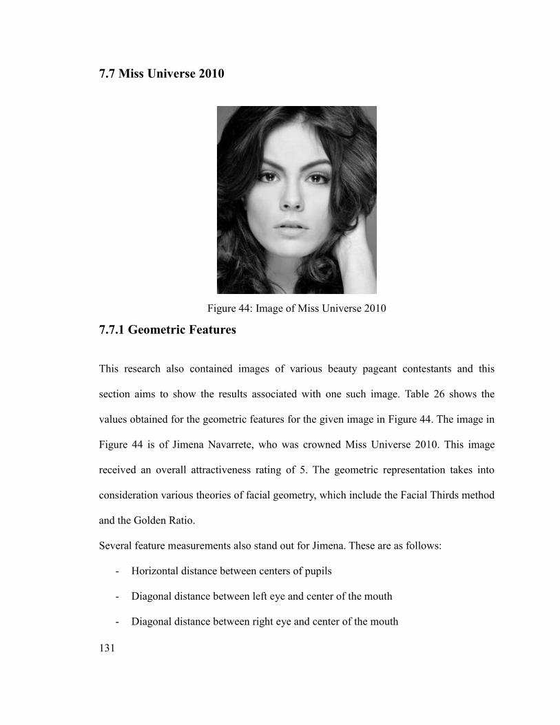
131
7.7 Miss Universe 2010
Figure 44: Image of Miss Universe 2010
7.7.1 Geometric Features
This research also contained images of various beauty pageant contestants and this
section aims to show the results associated with one such image. Table 26 shows the
values obtained for the geometric features for the given image in Figure 44. The image in
Figure 44 is of Jimena Navarrete, who was crowned Miss Universe 2010. This image
received an overall attractiveness rating of 5. The geometric representation takes into
consideration various theories of facial geometry, which include the Facial Thirds method
and the Golden Ratio.
Several feature measurements also stand out for Jimena. These are as follows:
- Horizontal distance between centers of pupils
- Diagonal distance between left eye and center of the mouth
- Diagonal distance between right eye and center of the mouth
132
- Vertical distance between top of forehead and chin
Measurement ID Description
Value for
Measurement(cm)
1 Vertical distance between top of
forehead and chin
5.74
2 Horizontal distance between outer
edges of cheekbones
3.79
3 Horizontal distance between outer
cheeks at the mouth
1.81
4 Vertical distance between eyebrow and
hair
1.71
5 Vertical length of upper head including
hair (not shown)
5.81
6 Vertical distance between pupil center
and eyebrow
1.17
7 Vertical distance between upper and
lower edge of eye
0.69
8 Horizontal distance between inner
corner and outer corner of the eye
1.41
9 Horizontal width of iris 0.42
10 Horizontal distance between centers of
pupils
3.79
11 Diagonal distance between left eye and
center of the mouth
3.60
12 Diagonal distance between right eye
and center of the mouth
3.39
Table 26: Values of sample geometric measurements
7.7.2 Textural Features
Table 27 displays a sample of the textural results that was obtained for the image shown
in Figure 44. These values shown are typical of values obtained for many other images in
the same attractiveness category as this image. The values of the third moment, R, and
Entropy are the generally lowest in comparison with the images that received a higher
attractiveness rating. This is mostly due to the presence of the lowest levels of variation
in the image.
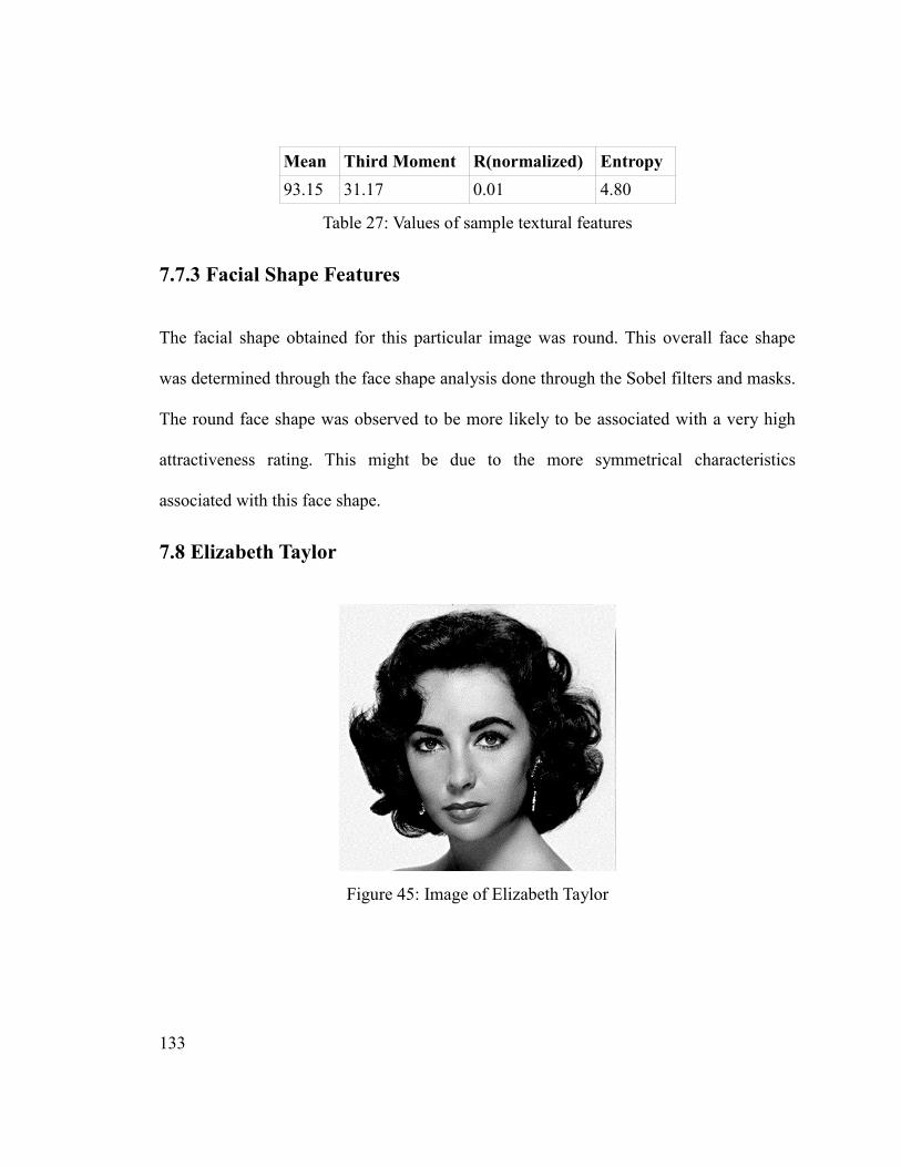
133
Mean Third Moment R(normalized) Entropy
93.15 31.17 0.01 4.80
Table 27: Values of sample textural features
7.7.3 Facial Shape Features
The facial shape obtained for this particular image was round. This overall face shape
was determined through the face shape analysis done through the Sobel filters and masks.
The round face shape was observed to be more likely to be associated with a very high
attractiveness rating. This might be due to the more symmetrical characteristics
associated with this face shape.
7.8 Elizabeth Taylor
Figure 45: Image of Elizabeth Taylor
134
7.8.1 Geometric Features
To help illustrate various levels of attractiveness, images of attractive actresses were
analyzed as part of this research. Table 28 shows the values obtained for the geometric
features for the given image in Figure 45. The image in Figure 45 is of Elizabeth Taylor,
who is a famous actress. This image received an overall attractiveness rating of 5. The
geometric representation takes into consideration various theories of facial geometry,
which include the Facial Thirds method and the Golden Ratio.
Several feature measurements also stand out for Elizabeth Taylor. These are as follows:
- Horizontal distance between centers of pupils
- Diagonal distance between left eye and center of the mouth
- Diagonal distance between right eye and center of the mouth
- Vertical distance between top of forehead and chin

135
Measurement ID Description
Value for
Measurement(cm)
1 Vertical distance between top of
forehead and chin
5.79
2 Horizontal distance between outer
edges of cheekbones
3.85
3 Horizontal distance between outer
cheeks at the mouth
2.23
4 Vertical distance between eyebrow and
hair
1.82
5 Vertical length of upper head including
hair (not shown)
5.89
6 Vertical distance between pupil center
and eyebrow
1.24
7 Vertical distance between upper and
lower edge of eye
0.69
8 Horizontal distance between inner
corner and outer corner of the eye
1.43
9 Horizontal width of iris 0.42
10 Horizontal distance between centre of
pupils
3.82
11 Diagonal distance between left eye and
center of the mouth
3.51
12 Diagonal distance between right eye
and center of the mouth
3.20
Table 28: Values of sample geometric measurements
7.7.2 Textural Features
Table 29 displays a sample of the textural results that was obtained for the image shown
in Figure 45. These values shown are typical of values obtained for many other images in
the same attractiveness category as this image. The values of the third moment, R, and
Entropy are the generally lowest in comparison with the images that received a higher
attractiveness rating; this is mostly due to the presence of the lowest levels of variation in
the image.
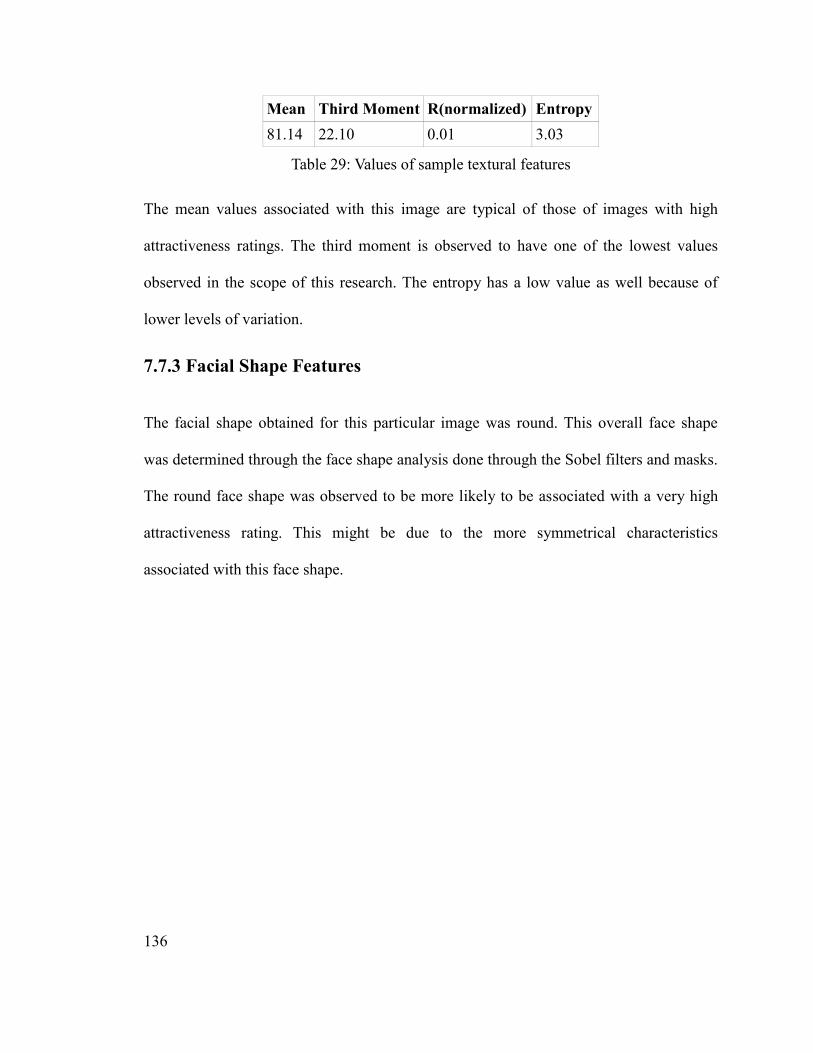
136
Mean Third Moment R(normalized) Entropy
81.14 22.10 0.01 3.03
Table 29: Values of sample textural features
The mean values associated with this image are typical of those of images with high
attractiveness ratings. The third moment is observed to have one of the lowest values
observed in the scope of this research. The entropy has a low value as well because of
lower levels of variation.
7.7.3 Facial Shape Features
The facial shape obtained for this particular image was round. This overall face shape
was determined through the face shape analysis done through the Sobel filters and masks.
The round face shape was observed to be more likely to be associated with a very high
attractiveness rating. This might be due to the more symmetrical characteristics
associated with this face shape.

137
7.9 Marilyn Monroe
Figure 46: Image of Marilyn Monroe
7.9.1 Geometric Features
To help illustrate various levels of attractiveness, images of attractive actresses were
analyzed as part of this research. Table 30 shows the values obtained for the geometric
features for the given image in Figure 46. The image in Figure 46 is of Marilyn Monroe,
who is a famous actress. This image received an overall attractiveness rating of 5. The
geometric representation takes into consideration various theories of facial geometry,
which include the Facial Thirds method and the Golden Ratio.
Several feature measurements also stand out for Marilyn Monroe. These are as follows:
- Horizontal distance between centers of pupils
- Diagonal distance between left eye and center of the mouth
- Diagonal distance between right eye and center of the mouth
138
- Vertical distance between top of forehead and chin
- Horizontal width of iris
- Vertical distance between eyebrow and hair
- Horizontal distance between outer edges of cheekbones
Measurement ID Description
Value for
Measurement(cm)
1 Vertical distance between top of
forehead and chin
5.82
2 Horizontal distance between outer
edges of cheekbones
3.91
3 Horizontal distance between outer
cheeks at the mouth
2.20
4 Vertical distance between eyebrow and
hair
1.71
5 Vertical length of upper head including
hair (not shown)
5.93
6 Vertical distance between pupil center
and eyebrow
1.29
7 Vertical distance between upper and
lower edge of eye
0.51
8 Horizontal distance between inner
corner and outer corner of the eye
1.41
9 Horizontal width of iris 0.91
10 Horizontal distance between centre of
pupils
3.61
11 Diagonal distance between left eye and
center of the mouth
3.39
12 Diagonal distance between right eye
and center of the mouth
3.11
Table 30: Values of sample geometric measurements
7.9.2 Textural Features
Table 31 displays a sample of the textural results that was obtained for the image shown
in Figure 46. These values shown are typical of values obtained for many other images in
the same attractiveness category as this image. The values of the third moment, R, and

139
Entropy are the generally lowest in comparison with the images that received a higher
attractiveness rating; this is mostly due to the presence of the lowest levels of variation in
the image.
Mean Third Moment R(normalized) Entropy
80.12 20.17 0.01 4.05
Table 31: Values of sample textural features
The mean values associated with this image are typical of those of images with high
attractiveness ratings. The mean is quite low indicating a good intensity distribution. The
entropy has a low value as well because of lower levels of variation. The value of R is
one of the lowest observed so far in the scope of this research.
7.9.3 Facial Shape Features
The facial shape obtained for this particular image was oval. This overall face shape was
determined through the face shape analysis done through the Sobel filters and masks. The
round face shape was observed to be most likely to be associated with a very high
attractiveness rating. This might be due to the most symmetrical characteristics associated
with this face shape.
140
Chapter 8 Conclusions and Future Work
This thesis has focused on the development of an automatic system for the analysis of
human facial beauty. This is done through the analysis of a given facial image and the
subsequent assignment of an attractiveness level to the particular image.
8.1 Conclusions
The data sets used for this research were sourced from various publicly available data sets
that are often used for research in image processing. These sets also included images
from a diverse and eclectic group of women, with varying levels of attractiveness. There
were a total of 215 images used for the purposes of this research. In order to establish the
ground truths for this research, an experimental survey was conducted. A diverse group of
48 participants agreed to take part in the research. The survey consisted of the
participants individually rating each image in the data sets to indicate their personal
rating of the attractiveness of the female in the image. These ratings were then analysed
for consistencies throughout the various individuals in order to assure the accuracy of
representation of the ratings. It was found that there were strong correlations and
consistencies within the ratings and this thus established to a great extent the accuracy of
the ratings.
The automatic facial beauty analysis system consisted of two main components; the first
part of which included the feature extraction and analysis of the given photograph and the
second part consisted of the training and testing of the machine learning system that
would be used for the prediction of attractiveness levels of any given image. Feature
selection was an integral constituent of the system as this determines that accuracy with

141
which any given image is represented. Therefore, the feature selection process had to
make sure the vital aspects related to beauty analysis were well represented in the
algorithm used for the identification of facial beauty.
The final feature vector converged to a set that consisted of features related to the key
aspects of human facial beauty, these included geometric features, textural features and
edge contour features as well. Another integral component of this research was the
application of active shape models for the accurate localization of facial features. This
was a novel approach in the area of facial beauty analysis as previous research has often
faced the difficulties of being able to accurately recognize key facial landmarks. Through
the use of active shape models, the accuracy of results was greatly improved to lead
towards an overall result of around 86%. The 14% were classified incorrectly mainly due
to various facial features being not fully incorporated into the facial representation due to
being blocked by hair. In addition, in various instances the hair obstructs the formation of
a clear facial outline.
8.2 Future Work
This research has aimed to provide a methodology for the analysis of human facial
beauty. This has been accomplished through incorporating various features for the
representation of facial beauty as well as making use of the machine learning techniques
that provide the most reliable and accurate results. There are, however, several future
additions that can be done to further the work already presented. A brief description of
these is as follows:
1. Incorporation of New Beauty Models: Several models have been carefully chosen

142
and represented in this research; these models were based on studies conducted in
the areas of aesthetics, sociology, and anthropology. However, the models can be
improved if the psychological aspect of human beauty is also taken into
consideration. Therefore, future work can also help to account for psychological
models of human facial beauty.
2. Incorporate Models for Various Cultures: This research has tried its best to include
images and respondents from all various cultures as possible. However, there are
several ethnicities that have not been represented in this research, which include
ethnicities from various regions of Africa. Future work could focus on the
addition of these ethnicities as well.
3. Addition of Methodology for Male Attractiveness: This research has focused on
only the attractiveness levels associated with females. However, of great interest
are also the attractiveness ratings associated with males. A possible focus of future
research could be models associated to human male attractiveness.
143
REFERENCES
[1] "Pots of Promise." The Economist 22 May 2003, http://www.economist.com/node/179
5852, retrieved 10 October 2012.
[2] Kringelbach, Morten, “The Human Orbitofrontal Cortex: Linking Reward to Hedonic
Experience,” Nature, Vol 6.1, (2005):691-673.
[3] AARABI, P., HUGHES, D., The automatic measurement of facial beauty, 2001 IEEE
International Conference on Systems, Man, and Cybernetics, Vol 12A, Page(s): 2644
-2647, 2001.
[4] John, Kirkland. “Categorical Perception of Facial Expressions of Emotion: Evidence
from Multidimensional Scaling.” Cognition and Emotion, Vol 3, Page(s): 112-142,
2001.
[5] Ying-Li,Tian, Takeo Kanade, “Recognizing Action Units for Facial Expression
Analysis,” IEEE Transactions on Pattern Analysis and Machine Intelligence, Vol
23.2, Page(s) 454-473, (2001).
[6] Kalkofen et al. “Kant’s “Facial Aesthetics” and Galton’s “Composite Portraiture” –
Are Prototypes beautiful?” Proceedings of the Xlth International Colloquium on
Empirical Aesthetics, Pages 23-45, 1990.
[7] Smithson, Craig. “ Francis Galton and Composite Portraiture.”Trans. S. H. Butcher.
Web Atomic and Massachusetts Institute of Technology, http://classics.mit.edu/
retrieved November 3, 2012.
[8] Jessica, Taubert. “The composite illusion requires composite face stimuli to be
biologically plausible.” Vision Research, Vol 49.14 Page(s) 215-220, (2009).
[9] Paulith, Mike. Composite Faces of the World. http://ultrafeel.tv/face-future/ , retrieved

144
9 December 2012.
[10] Buchala et al. “Global and Feature Based Gender Classification of Faces: A
Comparison of Human Performance and Computational Models,”IEEE
Transactions on Pattern Analysis and Machine Intelligence, Vol 13.5, Page(s) 134-
143, (2003).
[11] Baluja et al. “Boosting Sex Identification Performance.” International Journal of
Computer Vision Vol 71:1, Page(s) 117-221, (2007).
[12] Michael, Cunningham. "Measuring the physical in physical attractiveness: Quasi-
experiments on the sociobiology of female facial beauty." Journal of Personality
and Social Psychology, Vol 50:5, Page(s) 112-125, (1986).
[13] Cunningham et al."Their ideas of beauty are, on the whole, the same as ours":
Consistency and variability in the cross-cultural perception of female physical
attractiveness." Journal of Personality and Social Psychology, Vol 68:2, Pages 112-
129, (1995).
[14] Schmidhuber, Jurgen. "Facial Beauty and Fractal Geometry." Istituto Dalle Molle di
Studi sull Intelligenza Artificiale Resarch, Pages 35-41, (1998).
[15] CMU Multi-PIE Face Database. Fhttp://www.multipie.org/,retrievedebruary 10,
2013.
[16] Yale Face Database. http://vision.ucsd.edu/content/yale-face-database, retrieved
March 19, 2013.
[17] The Facial Recognition Technology (FERET) Database. <http://www.itl.nist.gov
/iad/humanid/feret/feret_master.html>, retrieved March 20, 2013.
[18] MIT Centre for Biological and Computational Learning Face Database.

145
<http://cbcl.mit.edu/software-datasets/FaceData2.html>, retrieved February 20,
2013.
[19] Essex Database. <http://cswww.essex.ac.uk/mv/allfaces/>, retrieved March 10, 2013.
[20] The Extended M2VTS Database. <http://www.ee.surrey.ac.uk/CVSSP/xm2vtsdb/>,
retrieved February 18, 2013.
[21] Martinez, Aleix. AR Face Database. <http://www2.ece.ohio-state.edu/~aleix/ARd
atabase.html> retrieved February 18, 2013.
[22] BioID Face Database. <http://www.bioid.com/index.php?q=downloads/softwa re/b
ioid-face-database.html>, retrived February 18, 2013.
[23] Computational Vision Database. <http://www.vision.caltech.edu/html-files/>,
retrieved February 18, 2013.
[24] Langlois et al. "Maxims or Myths of Beauty? A Meta-Analytic and Theoretical
Review." Psychological Bulletin 126:3, Pages 110-119, (2000).
[25] Khoo, Charlie. "Perceptions of Beauty in a Western Society." Changing Faces Vol 2,
Pages 24-29, (2009).
[26] Posamentier, Alfred. "The Pythagorean Theorem: The Story of Its Power and
Beauty." The Mathematical Intelligencer, Vol 34:3, Page(s) 94-116,(2012).
[27] Psychological Image Collection at Stirling. <http://pics.psych.stir.ac.uk/>, retrieved
March 12, 2013.
[28] McDonnell et al. "Application of the Golden Ratio to 3D Facial Models."
Eurographics Ireland Workshop Pages 56-61, (2003).
[29] Held, Dirk. "Eros, Beauty, and the Divine in Plato." New England Classic Journal
36:3, Pages 12-27, (2009).
146
[30] Early Theories of Beauty. <http://www2.uiah.fi/projects/metodi/15k.htm>, retrieved
April 10, 2013.
[31] Rhodes, Gillian. "The Evolutionary Psyhochology of Facial Beauty." Annual Review
Psychology Vol 57, pages 56-71(2006).
[32] Frazier, Christopher. Dynamic Beauty: Cultural Influences and Changing
Perceptions-Becoming Prettier or Erasing One's Own Culture?
http://hilo.hawaii.edu/academics/hohonu/documents/Vol04x02DynamicBeauty.pdf,
retrieved June 14, 2013.
[33] Zeki, Semir. "Art and the Brain." Daedalus, Vol 127:2, Page(s) 45-56, (2000).
[34] Langlois et al. "Facial Diversity and Infant Preferences for Attractive Faces."
Developmental Psychology 27:1, Page(s) 123-139, (1991).
[35] Langlois et al. "Attractive Faces are Only Average." Psychological Science Vol 1:2,
Page(s) 45-59,(1990).
[36] Miller, Arthur. " A Thing of Beauty." Perspectives, Vol 189:3, Page(s) 89-101,(2006).
[37] Zaidel et al. "Assymetry and Symmetry in the Beauty of Human Faces." Symmetry
2:1, Pages 125-138, (2010).
[38] Zaidel et al. "Appearance of Symmetry, Beauty, and Health in Human Faces." Brain
and Cognition 57Pages 135-147,(2005).
[39] Fink et al. "Skin Texture and Color and Attractiveness ." Journal of Comparative
Psychology Vol 12, Pages 71-84, (2001).
[40] Chen et al. "A Benchmark of Geometric Facial Beauty Study." Medical Biometrics,
Pages 61-65(2010).
[41] FEI Face Database. <http://fei.edu.br/~cet/facedatabase.html>, retrived March 10,

147
2013.
[42] Indian Face Database. <http://vis-www.cs.umass.edu/~vidit/IndianFaceDatabase/>,
retrieved March 10, 2013.
[43] Lopez et al. "Introducing the Golden Section to Computer Science." Proc. of the
First IEEE International Conference on Cognitive Informatics (ICCI02), Pages 131-
156, 2002.
[44] Farkas et al. "Vertical and Horizontal Proportions of the Face in Young Adult North
American Caucasians”. Plastic and Reconstructive Surgery Vol 75, Page(s) 92-101,
(1985).
[45] T.F Cootes, G.J. Edwards, C.J. Taylor. “Active Appearance Models.” Proc. of the
European Conference on Computer Vision, Vol. 2 , Page(s) 484-498 (1998).
[46] T.F Cootes, G.J. Edwards, C.J. Taylor. “Active Shape Models-Their Training and
Application.” Computer Vision and Image Understanding, Vol. 61 , Page(s) 38-59
(1995).
[47] T. F. Cootes, C. J. Taylor, D. H. Cooper, and J. Graham. “Training models of shape
from sets of examples”. In Proceedings of BMVC’92, Vol. 82 , Page(s) 266–275,
(1992).
[48] Michael Spira. “On the Golden Ratio”. Proc. of the International Congress on
Mathematical Education , Page(s) 23-34, (2012).
[49] L. Farkas & J. Kolar. “Anthropometrics and art in the aesthetics of women’s faces”.
Clinics in Plastic Surgery, Vol. 14: Page(s) 599–616, 1987.
[50] Y. Jefferson. “Facial aesthetics-presentation of an ideal face”. Journal of General
Orthodontics, Vol 4, Page(s) 18–23, 1993.
148
[51] B. Finka et al. “Visible skin color distribution plays a role in the perception of age,
attractiveness, and health in female faces”. Evolution and Human Behavior, Vol 27,
Page(s) 433–442, 2006.
[52] Mihran Tuceryan and Anil K. Jain. “Texture Analysis”. The Handbook of Pattern
Recognition and Computer Vision, Page(s) 207-248, World Scientific Publishing
Co., 1998.
[53] Dario Valenzano, Andrea Mennucci, Giandonato Tartarelli, Alessandro Cellerino.
“Shape Analysis of Female Facial Attractiveness”. Medical Biometrics, Vol 46:
Page(s) 1282-1291, 2006.
[54] Wenshuo Gao, Lei Yang, Xiaoguang Zhang, Huizhong Liu. “An Improved Sobel
Edge Detection”. IEEE International Conference on Cognitive Informatics
(ICCI02), Page(s) 100-115, 2010.
[55] James, David. “Anatomy of the Human Eye”. http://www.ic.uc sc.edu/~bruceb/ps
yc123/ Vision1 23.html.pdf, retrieved June 12, 2013.
[56] “Anatomy of Nose and Sinus”. http://ws.ajou.ac.kr/~ ent/knew/education/medical_
stud ent/lecture/ 05_nose_anatomy.pdf, retrieved May 5, 2013.
[57] K. I. Kim, K. Jung, S. H. Park, and H.J Kim, “Support vector machine-based text
detection in digital video”, Pattern Recognition, Vol. 34, Page(s) 527-529 (2001).
[58] Muller O'Rahilly, “The mouth, tongue, and teeth.” http://www.dartmouth.edu/
~humananato my /part_8/cha pter_51.html, retrieved March 9, 2013.
[59] E.Osuna, R.Freund, and F.Girosi, “Training support vector machines: an application
to face detection”, Proceedings CVPR'97, Page(s) 56-71, 1997.
[60] C.J.Lin, On the convergence of the decomposition method for support vector

149
machines, IEEE Transactions on Neural Networks, 12(6), 2001, Page(s) 1288-1298.
[61] T.Joachims, Advances in Kernel Methods: Support Vector Machines , Page(s) 52-
71, 1999.