a study of the critical viscosity model of friction stir

A STUDY OF THE CRITICAL VISCOSITY MODEL OF FRICTION STIR WELDING

IN RELATION TO TOOL FEATURES

By

Jacob Matthews

Thesis

Submitted to the Faculty of the

Graduate School of Vanderbilt University

in partial fulfillment of the requirements

for the degree of

MASTER OF SCIENCE

in

Mechanical Engineering

September 30, 2018

Nashville, Tennessee

Approved:

Alvin M. Strauss, Ph.D.

George E. Cook, Ph.D.

ii

DEDICATION

This thesis is dedicated to my family who have supported me in everything I have done and

made great personal efforts to give me opportunities they never had, to my wife for her

never-ending support through all the long nights at work, and to my son William who has

motivated me to work harder every day.

iii

ACKNOWLEDGMENTS

If I was asked if I would rather be the worst player on a winning team, or the best player

on a losing team, this experience has shown me the benefit of the former. To the smarter players

on the team who taught me so much along the way, thank you for all your time and expertise.

Gratitude is owed to Dr. Strauss and Dr. Cook for mentorship and guidance in a wider array of

topics than any two people should have. Specifically, I would like to thank Todd Evans for his

mentorship and overall guidance of the project, Adam Jarrell for help with instrumentation and

welding support, Kelsay Neely for her unmatched knowledge of material science, and Jay

Reynolds for his help with the welding program, and measuring topologies of the anvil and

specimen. Finally, the project would not have been possible without the financial support of

Vanderbilt University and the NASA Space Grant.

iv

TABLE OF CONTENTS

Page

DEDICATION .......................................................................................................................... ii

ACKNOWLEDGMENTS ..................................................................................................iii

LIST OF TABLES ...................................................................................................................... vii

LIST OF FIGURES ..........................................................................................................viii

Chapter

1 Introduction .................................................................................................................. 1

2 Heat Generation and Flow Modeling ........................................................................... 3

2.1 Rosenthal Solutions ............................................................................................ 3

2.2 Schmidt and Hattel Heat Generation Model ....................................................... 4

2.3 Mendez Heat Generation Model ......................................................................... 7

3 Material Flow Modeling ............................................................................................... 8

3.1 Colligan Material Flow Experiments ................................................................. 8

3.2 Reynolds Material Flow Experiments ................................................................ 8

3.3 Arbegast Extrusion Model .................................................................................. 8

3.4 Ulysse Material Flow Model .............................................................................. 9

3.5 Nunes Rotating Plug Model ............................................................................... 9

3.6 Pei and Dong Adiabatic Shear Band Model ...................................................... 10

3.7 Crawford Couette Flow Model ......................................................................... 12

3.8 Nandan Critical Viscosity Model ..................................................................... 14

3.9 Johnson-Cook Model ........................................................................................ 15

3.10 Zener-Hollomon Parameter and Hyperbolic-Sine Model .............................. 16

3.11 Onion Rings .................................................................................................... 16

3.12 Dynamic Recrystallized Zone Shape .............................................................. 18

3.13 Precipitate Depositing Effects ........................................................................ 19

4 Current Model ............................................................................................................. 20

4.1 Modelling Summary ......................................................................................... 20

4.2 Velocity Field Calculation ................................................................................ 22

4.3 Strain Rate Tensor ............................................................................................ 23

4.4 Critical Viscosity .............................................................................................. 23

4.5 Flow Band Width .............................................................................................. 24

v

5 Weld Parameter Mapping .......................................................................................... 27

5.1 Current Weld Parameter Metric ....................................................................... 27

5.2 Proposed Weld Parameter Metric ..................................................................... 29

6 Tool Components ....................................................................................................... 34

6.1 Shoulder ............................................................................................................ 34

6.2 Pin ..................................................................................................................... 34

6.3 Material ............................................................................................................. 36

7 Tool Component Features .......................................................................................... 37

7.1 Shoulder Scrolls ................................................................................................ 37

7.2 Pin Threads ....................................................................................................... 37

7.3 Triangular Pin ................................................................................................... 38

8 Experimental Configuration ....................................................................................... 39

8.1 Machine Setup .................................................................................................. 39

8.2 Anvil Topo ........................................................................................................ 40

8.3 Specimen Topo ................................................................................................. 41

8.4 Tools ................................................................................................................. 42

8.5 Weld Data ......................................................................................................... 43

8.6 Optical Testing Methods .................................................................................. 43

8.7 Tension Testing Methods ................................................................................. 44

9 Results ........................................................................................................................ 46

9.1 Flow Band Model Verification ......................................................................... 46

9.2 Axial Force ....................................................................................................... 52

9.3 Transverse Force ............................................................................................... 55

9.4 Torque ............................................................................................................... 57

9.5 Yield Strength ................................................................................................... 55

10 Discussion ................................................................................................................. 66

10.1 Tool Features Effect on Transverse Force ...................................................... 66

10.2 Tool Features Effect on Axial Force .............................................................. 67

10.3 Tool Features Effect on Torque ...................................................................... 68

10.4 Tool Features Effect on Yield Strength .......................................................... 69

10.5 Tool Features Effect on Dynamic Recrystallized Zone Shape ....................... 70

10.6 Tool Features Effect on Flow Band Width ..................................................... 72

10.7 Mechanical Conditions and Weld Parameter Map ......................................... 72

10.8 Thermal Expansion Controller ....................................................................... 73

10.9 Database .......................................................................................................... 73

vi

11 Conclusions .............................................................................................................. 76

REFERENCES ................................................................................................................. 83

LIST OF TABLES

vii

Table Page

Table 1 - Verification Weld Parameters and Results ..................................................................46

Table 2 - Flow Band Width by Tool Feature ..............................................................................52

Table 3 - Raw Specimen Test Data .............................................................................................63

Table 4 - Tool Result Analysis ....................................................................................................64

Table 5 - Specimen Location Result Analysis ............................................................................64

Table 6 - Percentage of Mean Strength by Specimen Location ..................................................65

viii

LIST OF FIGURES

Figure Page

Figure 1 - FSW Components ...........................................................................................................1

Figure 2 - Arbegast Flow-Partitioned Zones ...................................................................................9

Figure 3 - Adiabatic Shear Banding Grain Structure .....................................................................11

Figure 4 - Flow Band Width vs Rotation Rate ..............................................................................25

Figure 5 - Flow Band Width vs Transverse Rate ...........................................................................26

Figure 6 - Pei and Dong Welding Parameter Metric .....................................................................27

Figure 7 - New Welding Parameter Map .......................................................................................30

Figure 8 - Energy Deposition vs Strength......................................................................................32

Figure 9 - Generalized Welding Parameter Map ...........................................................................33

Figure 10 - TWI Trivex tool (a) and MX-Trivex tool (b) ..............................................................35

Figure 11 - VUWAL FSW Machine ..............................................................................................40

Figure 12 - Anvil Topography .......................................................................................................41

Figure 13 - Specimen Topography ................................................................................................42

Figure 14 - Tools used in experiments ...........................................................................................43

Figure 15 - Sample showing locations of tensile test specimen ....................................................45

Figure 16 - Verification Weld Etches ............................................................................................47

Figure 17 - Flow Band Width Calculations ...................................................................................48

Figure 18 - Verification Welds Rotation Rate vs Flow Band Width .............................................49

Figure 19 - Verification Welds Rotation Rate vs Flow Band Width .............................................50

Figure 20 - Energy Deposition vs Flow Band Width ....................................................................51

Figure 21 - Flow Band Prediction Error vs Energy Deposition.....................................................52

ix

Figure 22 - Raw Axial Force Weld Data .......................................................................................53

Figure 23 - Axial Force at Specimen Locations ............................................................................55

Figure 24 - Transverse Force ........................................................................................................56

Figure 25 - Transverse Force at Specimen Locations ....................................................................57

Figure 26 - Torque Minima and Maxima ......................................................................................58

Figure 27 - Torque at Specimen Locations ....................................................................................59

Figure 28 - PS 9545 Tensile Test Results ......................................................................................60

Figure 29 - TP 9545 Tensile Test Results ......................................................................................61

Figure 30 - TPS 9545 Tensile Test Results ...................................................................................61

Figure 31 - TPS 9545-t Tensile Test Results .................................................................................62

Figure 32 - Etches of Welds from Different Tools ........................................................................71

1

1. Introduction

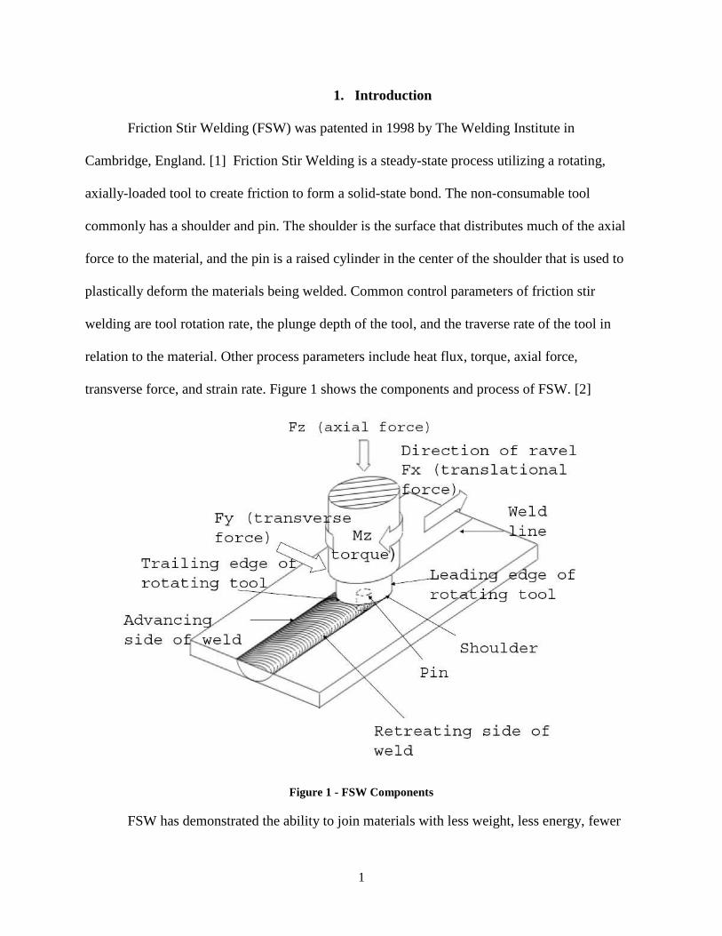
Friction Stir Welding (FSW) was patented in 1998 by The Welding Institute in

Cambridge, England. [1] Friction Stir Welding is a steady-state process utilizing a rotating,

axially-loaded tool to create friction to form a solid-state bond. The non-consumable tool

commonly has a shoulder and pin. The shoulder is the surface that distributes much of the axial

force to the material, and the pin is a raised cylinder in the center of the shoulder that is used to

plastically deform the materials being welded. Common control parameters of friction stir

welding are tool rotation rate, the plunge depth of the tool, and the traverse rate of the tool in

relation to the material. Other process parameters include heat flux, torque, axial force,

transverse force, and strain rate. Figure 1 shows the components and process of FSW. [2]

Figure 1 - FSW Components

FSW has demonstrated the ability to join materials with less weight, less energy, fewer

2

restrictions, and at higher strengths. FSW does not require filler materials, resulting in welds that

weigh less than traditional methods. This weight reduction and the ability to join higher strength

alloys like the 2000 and 7000 series of aluminum alloys makes FSW popular in the aerospace

industry. FSW requires less energy and is cheaper to operate than traditional methods requiring

large power supplies and filler materials. FSW is not restricted by materials, as it easily welds

materials difficult or impossible to weld using traditional methods like certain aluminums or

dissimilar metals. This makes welding of aluminum components to steel frames economical in

the automotive industry. The possibility of welding under water has been demonstrated and

theoretically possible in space, making it popular in the marine and space industries.

This thesis will discuss the basics of FSW modeling and layout the progress of FSW

models over time. This will include the progress of heat generation, material flow, the eventual

addition of localized material flow bands, and how weld seam input energy affects the

thermomechanical conditions of the weld. Welding parameter maps will be introduced that help

estimate correct welding parameters and how weld strengths are affected. The thesis will then

discuss tool features and how they may affect the thermomechanical conditions of the weld in

the context of the models and weld parameter maps discussed. To do this, it will explore a

simplified pseudo-model based on the idea that there is a critical viscosity that determines if the

material will flow and conduct several welds to verify that this model can predict the width of

material flowing around the pin. It will then outline the experiments conducted with four

different tool designs, discuss the results of these welds, and draw conclusions on how tool

features affect the thermomechanical conditions and strengths.

3

2. Heat Generation and Flow Modeling

2.1 Rosenthal Solutions

Rosenthal developed a thermal model for traditional arc welding. His model described

quasi-steady state temperature fields in a semi-infinite plate from a moving, line heat source. [3]

The Rosenthal equation is described in Equation 1. [3]

𝑇 = 𝑇∞ +𝑄 ∗ exp(

−𝑣 ∗ (𝑤𝑓𝑏 + 𝑟)2𝛼 )

2𝜋𝑘𝑟

Equation 1 - Rosenthal Equation

𝑄 ≡ ℎ𝑒𝑎𝑡𝑔𝑒𝑛𝑒𝑟𝑎𝑡𝑖𝑜𝑛

𝑣 ≡ 𝑡𝑟𝑎𝑛𝑠𝑣𝑒𝑟𝑠𝑒𝑣𝑒𝑙𝑜𝑐𝑖𝑡𝑦

𝑟 ≡ 𝑑𝑖𝑠𝑡𝑎𝑛𝑐𝑒𝑓𝑟𝑜𝑚ℎ𝑒𝑎𝑡𝑔𝑒𝑛𝑒𝑟𝑎𝑡𝑖𝑜𝑛𝑠𝑜𝑢𝑟𝑐𝑒(𝑝𝑖𝑛𝑎𝑥𝑖𝑠) 𝛼 ≡ 𝑡ℎ𝑒𝑟𝑚𝑎𝑙𝑑𝑖𝑓𝑓𝑢𝑠𝑖𝑣𝑖𝑡𝑦

𝑘 ≡ 𝑡ℎ𝑒𝑟𝑚𝑎𝑙𝑐𝑜𝑛𝑑𝑢𝑐𝑡𝑖𝑣𝑖𝑡𝑦

𝑤𝑓𝑏 ≡ 𝑓𝑙𝑜𝑤𝑏𝑎𝑛𝑑𝑤𝑖𝑑𝑡ℎ

Equation 2 describes the Peclet number. It describes the relative rates of heat transfer by

convection and conduction to determine if heat transfer is dominated by convection or

conduction. If this value is much less than one, it means that isotherms around the pin become

near circular and Rosenthal’s solutions are valid. Values greater than one indicate that forced

convection occurs at a significant magnitude. [4] [5]

𝑃𝑒 =𝜌𝑣𝑡𝐶𝑝𝐿𝑅

𝑘=𝑣𝑡𝑝𝑟2𝛼0

Equation 2 - Peclet Number

𝜌 ≡ 𝑚𝑎𝑡𝑒𝑟𝑖𝑎𝑙𝑑𝑒𝑛𝑠𝑖𝑡𝑦

𝑣𝑡 ≡ 𝑡𝑟𝑎𝑛𝑠𝑣𝑒𝑟𝑠𝑒𝑣𝑒𝑙𝑜𝑐𝑖𝑡𝑦

𝐶𝑝 ≡ 𝑠𝑝𝑒𝑐𝑖𝑓𝑖𝑐ℎ𝑒𝑎𝑡

𝐿𝑅 ≡ 𝑐ℎ𝑎𝑟𝑎𝑐𝑡𝑒𝑟𝑖𝑠𝑡𝑖𝑐𝑙𝑒𝑛𝑔𝑡ℎ𝑜𝑓𝑏𝑜𝑢𝑛𝑑𝑎𝑟𝑦𝑙𝑎𝑦𝑒𝑟𝑡ℎ𝑖𝑐𝑘𝑛𝑒𝑠𝑠

𝑘 ≡ 𝑡ℎ𝑒𝑟𝑚𝑎𝑙𝑐𝑜𝑛𝑑𝑢𝑐𝑡𝑖𝑣𝑖𝑡𝑦

𝑝𝑟 ≡ 𝑝𝑖𝑛𝑟𝑎𝑑𝑖𝑢𝑠

𝛼0 ≡ 𝑡ℎ𝑒𝑟𝑚𝑎𝑙𝑑𝑖𝑓𝑓𝑢𝑠𝑖𝑣𝑖𝑡𝑦𝑎𝑡𝑏𝑎𝑠𝑒𝑝𝑙𝑎𝑡𝑒𝑎𝑡𝑐𝑟𝑖𝑡𝑖𝑐𝑎𝑙𝑡𝑒𝑚𝑝𝑒𝑟𝑎𝑡𝑢𝑟𝑒

When FSW is referred to as a solid-state welding process, it distinguishes it from

traditional arc welding. In traditional arc welding, extreme heat creates a liquid form of the

4

materials to be joined. Several unwanted effects may result. Liquifying the materials

significantly changes the microstructure and lowers the weld strength. The extreme heat also

creates high residual stresses in the materials. This process does not work for some metals and

does not work for many dissimilar metals and plastics. Solid-state welding joins materials that

maintain their form as a solid. FSW does this by maintaining temperatures under the material’s

solidus temperature and applying pressure and high strain rates.

Modeling the process of FSW has proven elusive over its almost three-decade history,

despite the dramatic increase in computing power over the same time. It is understood that the

material state is in a plastic region somewhere between solid and liquid. Some techniques have

tried to adapt solid mechanics techniques to describe the process, and some have tried adapted

fluid mechanics approaches. Two main questions dominate the modeling efforts today: Is the

peak temperature dominated by heat generation from friction or plastic dissipation and is

material plasticized by the formation of adiabatic shear bands or a decrease of viscosity below a

critical value?

The dominant question in thermal models is whether the peak temperature is dominated

by heat generated from friction or plastic dissipation. Another way to characterize this question

is by determining the velocity of material at the tool interface. Three described possibilities are:

sticking, slipping, or partial sliding and sticking.

2.2 Schmidt and Hattel Heat Generation Model

In a slipping condition, the material velocity near the tool is zero, meaning the tool

rotation does not cause any deformation and only creates frictional heat caused by the contact of

two metals sliding past each other. This condition will occur if the contact shear stress is less

than the material yield shear stress. The material will deform slightly but will remain elastic. [6]

5

In a sticking condition, a boundary layer of material is formed around the pin. The

material nearest the tool travels the same speed as the tool, creating a boundary layer of

intermediate velocities within a band until the material velocity is zero again. This condition is

valid where the frictional shear stress is greater than the yield shear stress of the material. [6]

In the remaining possible condition, a combination of both are present. Like in the

sticking condition, a boundary layer is created in the material. Unlike the sticking condition, the

velocity of material nearest the pin will be traveling at a velocity below the tool velocity. In this

case, a dynamic contact shear stress equals the material shear yield stress and comes to an

equilibrium dependent on the plastic deformation rate. [6]

The contact state variable, 𝛿, describes whether the tool is sticking, slipping, or the

amount of partial sticking. It is defined as the material velocity nearest the pin divided by the tool

velocity, Equation 3. [6]

𝛿 =𝑣𝑚𝑎𝑡𝑒𝑟𝑖𝑎𝑙

𝑣𝑡𝑜𝑜𝑙

Equation 3 - Contact State Variable

A value of one would describe sticking, while a value of zero would describe slipping.

Schmidt et al concluded that the contact state variable was one or very near one, indicating that a

sticking condition is most likely [6].

Schmidt and Hattel are often cited for developing the generally adopted equation for total heat

generation, Equation 4. [6]

6

𝑄𝑡𝑜𝑡𝑎𝑙 = 𝛿𝑄𝑠𝑡𝑖𝑐𝑘𝑖𝑛𝑔 + (1 − 𝛿)𝑄𝑠𝑙𝑖𝑑𝑖𝑛𝑔

=2

3𝜋𝜔[𝛿𝜏𝑦𝑖𝑒𝑙𝑑 + (1 − 𝛿)𝜇𝑝][(𝑅𝑠ℎ𝑜𝑢𝑙𝑑𝑒𝑟

3 − 𝑅𝑝𝑟𝑜𝑏𝑒3 )(1 − 𝑡𝑎𝑛 𝛼) + 𝑅𝑝𝑟𝑜𝑏𝑒

3 + 3𝑅𝑝𝑟𝑜𝑏𝑒2 𝐻]

Equation 4 - Heat Generation Equation

𝛿 ≡ 𝐶𝑜𝑛𝑡𝑎𝑐𝑡𝑆𝑡𝑎𝑡𝑒𝑉𝑎𝑟𝑖𝑎𝑏𝑙𝑒(𝑑𝑖𝑚𝑒𝑛𝑠𝑖𝑜𝑛𝑙𝑒𝑠𝑠𝑠𝑙𝑖𝑝𝑟𝑎𝑡𝑒) 𝜏𝑦𝑖𝑒𝑙𝑑 ≡ 𝑀𝑎𝑡𝑒𝑟𝑖𝑎𝑙𝑌𝑖𝑒𝑙𝑑𝑆𝑡𝑟𝑒𝑠𝑠𝑎𝑡𝑤𝑒𝑙𝑑𝑖𝑛𝑔𝑡𝑒𝑚𝑝𝑒𝑟𝑎𝑡𝑢𝑟𝑒

μ ≡ FrictionCoefficient p ≡ UniformPressureatcontactinterface 𝜔 ≡ 𝐴𝑛𝑔𝑢𝑙𝑎𝑟𝑅𝑜𝑡𝑎𝑡𝑖𝑜𝑛𝑆𝑝𝑒𝑒𝑑 𝛼 ≡ 𝐶𝑜𝑛𝑒𝐴𝑛𝑔𝑙𝑒

𝑅𝑠ℎ𝑜𝑢𝑙𝑑𝑒𝑟 ≡ 𝑆ℎ𝑜𝑢𝑙𝑑𝑒𝑟𝑅𝑎𝑑𝑖𝑢𝑠 𝑅𝑝𝑟𝑜𝑏𝑒 ≡ 𝑃𝑟𝑜𝑏𝑒𝑜𝑟𝑃𝑖𝑛𝑅𝑎𝑑𝑖𝑢𝑠

𝐻 ≡ 𝑃𝑟𝑜𝑏𝑒𝑜𝑟𝑃𝑖𝑛𝐻𝑒𝑖𝑔ℎ𝑡

This early research recognized that as the temperature approaches the solidus temperature

and acts more like a liquid, the yield stress decreases and consequently generates less heat. While

Schmidt and Hattel’s model neglects strain-rate dependence in the material flow model, they

identified that the process is self-regulating to a degree. Heat from plastic dissipation depends on

the material’s flow stress at the current temperature, the strain, and the strain rate. The contact

stress will be equal to the material yield shear stress during steady-state conditions. [7]

Assuming a sticking condition, the contact state variable equals one and the contact shear

stress is estimated to be the material yield stress divided by the square root of three. Equation 5

represents the resulting equation for heat generation assuming a sticking condition for a flat

shouldered, threadless pin tool. [6]

𝑄𝑡𝑜𝑡𝑎𝑙 =2

3𝜋𝜔

𝜎𝑦𝑖𝑒𝑙𝑑

√3[(𝑅𝑠ℎ𝑜𝑢𝑙𝑑𝑒𝑟

3 − 𝑅𝑝𝑟𝑜𝑏𝑒3 )(1 − 𝑡𝑎𝑛 𝛼) + 𝑅𝑝𝑟𝑜𝑏𝑒

3 + 3𝑅𝑝𝑟𝑜𝑏𝑒2 𝐻]

Equation 5 - Heat Generation from Sticking Condition

Separating Equation 5 into heat generation from shoulder, probe shoulders, and probe

bottom allows contributions from each to be quantified. Schmidt and Hattel determined heat

generation to be 83% from the shoulder, 16% from the probe sides, and 1% from the probe tip

for AL 7075 and 86% from the shoulder, 11% from the probe sides, and 3% from the probe tip

for AL 2024 [7]. Analytical estimates for tools with threaded probes by Colegrove estimate heat

7

generation from the probe as high as 20%. [8]

2.3 Mendez Heat Generation Model

Mendez et al. noted that the heat generation from the shoulder does not significantly

affect the peak temperature near the pin. The shoulder acts as a distributed, pre-heating

mechanism that initially softens material, but does not significantly affect the plasticization of

the metal. The peak temperature is dominated by plastic dissipation by the pin. This insight

allowed modeling to uncouple shoulder heat generation from pin plastic dissipation heat

generation. [5]

8

3. Material Flow Modeling

3.1 Colligan Material Flow Experiments

Colligan first attempted to measure material flow by imbedding steel balls into a butt

weld of AL 6061 and AL 7075 to act as tracers. Steel balls that struck the pin on the advancing

side of the weld were deposited on the retreating side behind the pin. Steel balls that struck the

pin on the retreating side of the weld were also deposited on the retreating side behind the weld.

Small vertical displacements towards the shoulder were observed. He concluded that material

flow behind the pin was characterized by both “stirring” and extrusion. The material on the

advancing side was stirred into the void by the pin, and the material on the retreating side was

extruded between the pin and the parent material. [9]

3.2 Reynolds Material Flow Experiments

Reynolds used a similar tracer technique but used thin sheets of AL 5054 during a butt

weld of AL 2195. He used the data to create 3D maps of the flow to improve visualization of the

material flow. He concluded that the material was extruded on both sides of the pin and that the

role of the pin was to provide frictional heating to create the conditions for successful extrusion.

[10]

3.3 Arbegast Extrusion Model

Arbegast suggested an extrusion model that divided the material up into four zones. Zone

I was material on the advancing side near the pin, Zone II was material on the retreating side

near the pin, Zone III is material dominantly influenced by the shoulder, and Zone IV was the

material underneath the pin he called the “Vortex Swirl Zone”. The zones were coupled into a

system where motion of material from one zone affected motion of material in an adjacent zone.

[11]

9

Figure 2 - Arbegast Flow-Partitioned Zones

3.4 Ulysse Material Flow Model

Ulysse introduced a model that related the deviatoric stress tensor to the strain-rate

tensor. This assumes that the material is a rigid-visco-plastic material highly dependent on

temperature and strain rates. This led to the conclusion that flow stress is the requirement driving

material flow, and that it can be solved for using an inverse hyperbolic-sine relationship and the

Zener-Hollomon parameter [12]. The Zener-Hollomon parameter represents temperature-

compensated strain rate [4]. This method was used by Sellars and Tegart [13] and was modified

by Sheppard and Wright [14]. It treats the material like a viscous non-Newtonian fluid with

negligible strain hardening effects. [15]

3.5 Nunes Rotating Plug Model

Nunes et al. suggest that a “plug” of material rotates at the same velocity as the pin and

travels with the tool. The width of this plug of material is at a maximum at the retreating edge

and can be approximated by Equation 6.

10

𝑤𝑠𝑏 =2𝑣𝑡𝜔

Equation 6 - Nunes Shear Band Width [16]

The idea that material is rotating with the pin has been widely accepted, though the cause

has not been agreed upon. The different models can be categorized as adiabatic shear bands,

Couette flow, and viscosity. These models are summarized in the following sections.

3.6 Pei and Dong Adiabatic Shear Band Model

Adiabatic shear bands are possible in materials with microstructural inhomogeneities or

defects. [17] For example, pure aluminum does not have microstructural inhomogeneity, and has

not been reported to experience shear bands. Aluminum alloys create microstructural

inhomogeneities and allow shear bands to form. High strain gradients are a principal cause for

shear band formation. Observations suggest that high strain rates cause massive elongation of

grains along the shear band propagation path, orientation of the elongated grains along shear

flow direction, and eventual fragmentation of the grains into smaller grains. [17]

11

Figure 3 - Adiabatic Shear Banding Grain Structure

A significant increase in the material strength over strain rates of about 10,000 𝑠−1 occurs

and is caused by a change in dislocation motion mechanism. At low strain rates, the deformation

rate is thermally activated. At these low strain rates, influence of the temperature of the material

on flow stress can be neglected. At high strain rates, the glide kinetics are controlled by viscous

phonon and electron drag. [18] This means at high strain rates, heat generation due to plastic

dissipation occurs and thermally softens the local material. Since flow stress is dependent on

temperature and strain rate, multiple phenomena are present.

The flow strength increases due to higher strain rates but decreases due to temperature.

Overall, the local rise in temperature due to plasticization dominates and greatly reduces the flow

stress where strain rates are high. This means that shear bands require strain rates of greater than

10,000 𝑠−1 to form. [18] Shear bands are highly influenced by the strain hardening ability of the

material. A material with a higher strain hardening ability requires a higher temperature for

12

thermal effects to start dominating strain rate effects and vice versa. [19] Adiabatic shear bands

are harder than the associated bulk material but are also more prone to cracking. They can be

eliminated from a material’s microstructure through heat treatment. [17]

Pei and Dong initially assumed that the material behavior can be modeled by the

Johnson-Cook law because of its dependency on temperature, strain, and strain rate. This model

predicted temperatures above the melting point of the material which experimental results show

to be unlikely. They suggest that this temperature increase is from the strain-hardening term,

which hot forming research has found to be minimal at temperatures present in FSW. [19]

Pei and Dong proposed an interesting model of shear localization in relation to FSW

parameters. They only considered the process during one revolution of the tool at steady state.

As the tool begins its rotation, the slipping condition is assumed. Frictional heat generation

causes thermal softening according to the Zener-Hollman model and the material near the pin

begins to change to a sticking condition. The velocity of the material near the pin quickly

approaches the velocity of the tool causing high strain and strain rates. The heat generation due

to Coulomb friction disappears and localized heat generation due to plastic dissipation

dominates.

The localized plastic heat generation continues to plasticize material and the width of the

shear band of material traveling at the velocity of the pin increases. To satisfy mass balance and

continuity conditions, the width of the shear band must be greater than or equal to the width of

the void created by the pin. If the shear band width is less than the max material flow, void

defects are predicted. [20]

3.7 Crawford Couette Flow Model

Crawford compared a traditional thermo-viscoplastic model to a Couette Flow model

13

originally developed by North et al. The Couette Flow Model is a fluid mechanics approach that

describes the flow of a viscous fluid between two plates. In the case of friction stir welding, the

plates are concentric cylinders. The inner cylinder is the tool, and the outer cylinder is the parent

material. The distance between the two plates is the width of the “third body region”, what is

referred to in this thesis as the shear band thickness. This distance is described by Equation 7. [2]

𝑊𝑟 =𝛼

𝛽𝜑2 + 𝑟𝑝𝜑 + 1

Equation 7 - Crawford Third Body Region Width

𝛼 =1

2(𝑟𝑝 − 𝜆𝛿2)

𝛽 =𝑟𝑠2 − 𝑟𝑝

2

ℎ𝑝𝜆

𝜑 =𝜔

𝑣𝑓

𝛿2 ≡ 𝑝𝑟𝑜𝑗𝑒𝑐𝑡𝑒𝑑𝑡ℎ𝑟𝑒𝑎𝑑𝑎𝑟𝑒𝑎

𝜆 ≡ 𝑛𝑢𝑚𝑏𝑒𝑟𝑜𝑓𝑡ℎ𝑟𝑒𝑎𝑑𝑠𝑝𝑒𝑟𝑖𝑛𝑐ℎ

Crawford also modeled the torque in FSW. The welding power is equal to the torque

multiplied by the rotation rate. The welding torque can be broken down to represent torque from

the pin and torque from the shoulder. The first term of Equation 8 represents torque from the

shoulder, and the last two terms represent the torque contribution of the pin. [2]

𝑀 = ∫ 2𝜋𝑟𝜎𝑑𝑟𝑟𝑠

𝑟𝑝

+ 2𝑟𝑝2ℎ𝑝𝜎 +∫ 2𝜋𝑟2𝜎𝑑𝑟

𝑟𝑝

0

Equation 8 - Welding Torque

r ≡ radius 𝜎 ≡ 𝑎𝑥𝑖𝑎𝑙𝑠𝑡𝑟𝑒𝑠𝑠 𝑟𝑝 ≡ 𝑝𝑖𝑛𝑟𝑎𝑑𝑖𝑢𝑠

ℎ𝑝 ≡ 𝑝𝑖𝑛ℎ𝑒𝑖𝑔ℎ𝑡

𝑟𝑠 ≡ 𝑠ℎ𝑜𝑢𝑙𝑑𝑒𝑟𝑟𝑎𝑑𝑖𝑢𝑠

If we neglect the torque from the pin’s bottom as negligible, then the torque from the pin

is represented by Equation 9. [2] Crawford concluded that the pin’s contribution to torque

represented roughly a fourth of the total torque required by the machine.

14

𝑀𝑝 = 2𝑟𝑝2ℎ𝑝𝜎

Equation 9 - Torque Contribution of Tool Pin

Crawford ultimately concluded that the Couette Flow Model works best for high weld

pitch welds, defined as the rotation rate divided by the translational rate. Overall, the visco-

plastic model was more accurate over a broad range of weld pitches. At higher weld pitches, the

Couette flow becomes more predictive than the visco-plastic model high temperatures increase

the material’s ability to flow. Couette flow likely works best as material acts more like liquid, but

less at lower temperatures.

3.8 Nandan Critical Viscosity Model

Nandan proposed a model for material flow that is dependent on the viscosity of the

material. The temperature and strain rate of the material lower the viscosity of the metal until a

critical viscosity is reached allowing material to flow. Once the material flows, forces on the

material are released, temporarily lowering both temperature and strain rates until the viscosity

rises above the critical viscosity and the process restarts. The iterative process results in the

banded structure known as onion rings behind the weld zone. [4]

Viscosity can be found with just knowledge of the flow stress and strain rate in Equation

13 and Equation 16. The viscosity was found to be dependent on both strain rate and

temperature, but strain rate was a more dominant factor for FSW thermo-mechanical conditions.

Nandan et al. determined the critical viscosity for AL6061-T6 to be 5x106 Pa-s. This value was

confirmed by Franke et al. [21]

𝜇 =𝜎𝑓

3휀̇

Equation 10 – Viscosity

휀̇ ≡ strainrate

𝜎𝑓 ≡ flowstress

The critical viscosity model is differentiated from the adiabatic shear band model by the

15

method of material transport. While strain rate contributes to material flow for both models,

adiabatic shear bands suggest strain rate dominates the material flow process and causes a

change in dislocation mechanism and is influenced by strain hardening. FSW likely involves a

range of microphysical processes involved in both elastic and anelastic deformation. [22] The

critical viscosity model suggests more of a balance between strain rate and temperature that is

thermally activated by the heat generated by plastic dissipation and is not affected by strain

hardening. Small shear bands may be forming, but they are on a small scale and do not dominate

material flow.

3.9 Johnson-Cook Model

There are many models of material strength at high pressures and strain rates. Johnson-

Cook, Zerilli-Armstrong, mechanical threshold stress, thermal activation phonon drag,

Steinberg-Lund, Steinberg-Guinan, and Preston-Tonks-Wallace to name a few. [23] Most

research in relation to FSW has focused on the Johnson-Cook model because of its applicability

to high strain rate loading and its ease of use. The Johnson-Cook model determined material

parameters over a relatively low range of strain, strain rate, and temperature data. This leads to

yield stresses much larger than experimental data at plastic strain values of 100-200 at room

temperature. This suggests that the Johnson-Cook is a strain hardening dominated material

model, but hot forming research suggests that material at temperatures approximate to FSW

show little evidence of strain hardening ability. [19] Assuming that plasticization is occurring,

then Equation 11 represents the flow stress according to the Johnson-Cook model. [18]

16

𝜎𝑓 = (𝐴 + 𝐵휀𝑝𝑙𝑛 )(1 + 𝐶 ln

휀�̇�𝑙

휀0̇)(1 − 𝑇∗𝑚)

Equation 11 - Flow Stress

𝐴 ≡ elasticlimitstrength

𝐵, 𝐶, 𝑛,𝑚 ≡ empiricalfitconstants 𝑇∗ ≡ homologoustemperature(ratiooftemperaturetomeltingtemperature) 휀 ≡ effectiveplasticstrain

휀̇ ≡ effectiveplasticstrainrate

3.10 Zener-Hollomon Parameter and Hyperbolic-Sine Model

Ulysse introduced a model that related the deviatoric stress tensor to the strain-rate

tensor. This assumes that the material is a rigid-visco-plastic material highly dependent on

temperature and strain rates. This lead to the conclusion that flow stress is the requirement

driving material flow, and that it can be solved for using an inverse hyperbolic-sine relationship

and the Zener-Hollomon parameter. [12] The Zener-Hollomon parameter represents temperature-

compensated strain rate. [4] This method was used by Sellars and Tegart [13] and was modified

by Sheppard and Wright [14]. It treats the material like a viscous non-Newtonian fluid with

negligible strain hardening effects. The temperature is calculated using Equation 1.

𝑍 = 휀̇𝑒𝑄𝑅𝑇

Equation 12 - Zener-Hollomon Parameter

휀̇ ≡ strainrate

Q ≡ temperature − independentactivationenergy

𝑅 ≡ gasconstant 𝑇 ≡ temperature

𝜎𝑓 =1

𝛼sinh−1(

𝑍

𝐴)1𝑛

Equation 13 - Hyperbolic Sine Relationship for Flow Stress

𝛼 ≡ 𝑡ℎ𝑒𝑟𝑚𝑎𝑙𝑑𝑖𝑓𝑓𝑢𝑠𝑖𝑣𝑖𝑡𝑦

𝑛, 𝐴 ≡ 𝑒𝑚𝑝𝑖𝑟𝑖𝑐𝑎𝑙𝑓𝑖𝑡𝑐𝑜𝑛𝑠𝑡𝑎𝑛𝑡𝑠

3.11 Onion Rings

The banded structure left behind welds is often referred to as “onion rings”. The banded

structure is formed by alternating layers of high strain rate bands and average strain rate bands

17

deposited into the void behind the pin. [24] These different bands have also been explained by

high strain rate bands on the advancing side of the weld and extruded material on the retreating

side of the weld. [25]

At high rotational rates and low transverse rates, onion ring structures cover a small

width of the weld and have irregular material flow including chunks of sheared parent material.

As translational rate increases, material flow becomes more regular and onion ring structures

extend further across the weld until an optimal translation rate is reached and then begin to

recede. [26]

Onion ring bands have thickness approximately equal to tool’s transverse advance per

revolution for cylindrical tools. This thickness is divided by the number of faces of the pin for

non-cylindrical tools (three for triangular tools for example). [24] When this value is small, the

distance between onion ring bands is small and it is difficult for the plasticized material to be

deposited because the area between the tool and the previous band is too small. As this value

increases, more plasticized material can be deposited across the width of the weld. This

phenomenon depends mainly on the shape of the tool’s pin and not on whether a sticking or

slipping condition is present. [26]

Onion ring structures start on the retreating side and compete with tunnel defects

originating on the advancing side of the weld. More pronounced onion ring structures mean

fewer tunnel defects in the weld. After material passes by the pin, the void behind the pin creates

a “low pressure zone” that exerts a force on the material towards it. If the material is not fluid

enough to flow into the void, void defects are formed. More pronounced onion rings may signal

that enough plasticized material is being produced to fill the void behind the pin and avoid tunnel

defects. [24]

18

An oscillation in the axial force applied to the material occurs during welding. The

frequency has been found to be equal to the rotation rate per second times the number of faces of

the tool (i.e. 1 for a circle, three for a triangle). This suggests that the deposition of material into

the void behind the tool causes a momentary reduction in forces required until the void has been

filled. The efficiency of material deposition can therefore be inferred by the regularity and

frequency of this oscillation in welding forces. [24] [27]

Onion rings must not be confused with flow band widths. Onion rings are dominated by

the shoulder and only occur if there is transverse movement. There is still plastic material flow

with spot welding, even though there is no onion ring formation. Onion rings are likely formed

when excess plastic material escapes consolidation and is wiped by the shoulder behind the weld.

An absence of onion rings in a weld means that not enough plastic material is being formed. Too

much plastic material will form flash. The correlation between onion rings and flow band width

ends there. There is no proof of a proportional relationship between onion ring width and flow

band width.

3.12 Dynamic Recrystallized Zone Shape

At lower welding speeds, the shape of the weld zone tends to be basin shaped. At higher

welding speeds the shape tends more towards a round or ellipsoidal shape. [28] This could

signify the impact that the shoulder has on the weld beneath. At lower transverse speeds, the

shoulder can deposit more energy into the weld, but the basin shape signifies that this depth is

limited. At higher transverse speeds, this energy does not have as much time to deposit and the

weld zone narrows.

This behavior of the weld zone seems to indicate that plasticization is due to viscosity of

the material and not adiabatic shear bands. At higher rotation rates, shear rates are expected to

19

increase, and shear band widths should increase. This relationship should not be affected much

by translational velocity. This does not appear to be represented experimentally. It is more likely

that an increase in temperature from an increase in heat generation at the shoulder is decreasing

the viscosity of the material, allowing it to flow in the weld zone. At high transverse velocities,

the shoulder heat generation does not have time to conduct in the z direction, resulting in an

ellipsoid. At low transverse velocities, more heat generation can reach deeper into the weld, and

the diameter of the weld nugget approaches the diameter of the tool shoulder.

3.13 Precipitate Depositing Effects

One last detail on material flow is the impact of precipitates on weld strength. It has been

observed that at low transverse rates or to a lesser degree high rotation rates, coarse Mg2Si

precipitates tended to dominate the tensile fracture mode of AL 6061. This may be caused by

high energy deposition values melting the material and allowing these precipitates to flow to the

outside of the weld zone. This disruption in microstructure lead to lower yield strengths at the

edge of the weld zone on the retreating side. [28]

20

4. Current Model

4.1 Modelling Summary

The purpose of discussing the progression of models for FSW in this thesis is not to delve

deeply and develop another model. The purpose is to discuss all the conceptual models and unify

concepts that appear to be experimentally proven to develop simple algebraic formulas based on

the welding parameters that can predict steady state conditions during the weld. There are two

large questions that define how the process of FSW occurs: Does heat generation occur through

plastic dissipation or solely through frictional heating and can material flow be modeled as a

solid or a liquid?

So far, this thesis has suggested that heat generation can occur as both friction and plastic

dissipation, and that material flow can be modeled as both a solid and a liquid, depending on the

welding parameters that create the welding thermo-mechanical environment. Therefore, this

thesis will make assumptions for the optimal thermo-mechanical environment. This thesis

assumes a sticking condition at tool interface, a heat generation model according to Equation 5,

the material yields at a flow stress that can be calculated by Equation 13, and that material is

deposited into the void through extrusion of high strain rate material on the advancing side and

extrusion of lower strain rate material on the retreating side.

It is possible that the pin has a slipping condition for part of every revolution, or it may

have several slipping revolutions before returning to a sticking condition. It is expected that the

process is self-regulating to a degree. As the material is plasticized by high strain rates possible

because of high pressure between the tool and the material, the material viscosity decreases and

there is less pressure between the tool and the material. Additionally, when material is deposited

into the void, this would also reduce the pressure between the tool and the material, leading to a

21

slipping condition. Nevertheless, a return to a sticking condition is assumed because the sticking

condition causes the dominant influence on temperature near the pin and is the dominant

influence on material flow outside of extrusion.

The heat generation model may not be the most accurate model, but it is assumed that it

is accurate enough to model heat deposition at steady state. The key concepts behind the model

is that it assumes a sticking condition and that shoulder heat generation can be thought of as a

preheating mechanism for the weld, and that the pin generates heat from plastic dissipation that

dominates the temperature near the tool. This model can be used to determine if excess heat is

being produced in the weld. If excess heat is produced, it is assumed that the material changes

state, and can more accurately be represented as a liquid. This change of state will decrease

resulting weld strength. The temperature, like the contact condition, is self-regulating, though. If

excess heat is produced, the viscosity of the material decreases until the material flows, which

decreases the plastic heat dissipation and the resulting temperature. This model assumes that the

process self-regulates around the solidus temperature of AL 6061, 852K.

Adiabatic shear bands are not likely created during FSW. As already discussed, they

require strain rates of 10,000 𝑠−1. Peak strain rates reported are between 1.7 and 1000 𝑠−1. [15]

Even at the largest strain rate reported, adiabatic shear bands are not likely to occur, though the

temperature compensated strain rates (Zener-Hollomon Parameter) is on the order of 1x109 from

experimental calculations. Expected shapes of the weld zone at higher strain rates do not follow

expectations of adiabatic shear band growth. There is a band of material that surrounds the pin

and travels at the same velocity, but there is no evidence to support that this material was formed

by the process of adiabatic shear banding.

The flow stress calculation in Equation 13 assumes that the machine is applying torque

22

until the material yields, and that the flow stress can be inferred from this torque by assuming

that 25% of the torque is from the pin. If the torque is not known, this thesis assumes that the

temperature self-regulates around the solidus temperature. Some peak temperatures reported are

reportedly at or higher than 98% the solidus temperature and support this hypothesis. [15] The

flow stress is then calculated at just under the solidus temperature and the strain rate is iterated at

different flow band widths and the result used to calculate viscosity until the viscosity converges

to the critical viscosity. We can calculate the strain rate based on velocity of the material.

Viscosity can then be solved for using Equation 10.

The strength of the weld is highly dependent on the weld’s ability to deposit material into

the void behind the pin. It is assumed that higher strength welds maintain a temperature below

but near the solidus temperature. The material is frictionally heated until it flows, and enough

plasticized material flows to fill the void behind the pin. If too much heat is deposited into the

weld, this material becomes weaker due to a phase change in the plasticized material leading to

lower strength welds. If enough heat is not deposited into the weld, not enough material

plasticizes to fill the void behind the pin leading to tunnel defects.

4.2 Velocity Field Calculation

The material velocity equations used in this thesis are the same used by Nandan [4]. This

model accounts for material recirculation and a range of tool slip values dependent on the

rotational speed and distance from the pin. These equations also account for the possibility of

Friction Stir Spot Welding (FSSW) in which a tool plunges but does not translate. The tool

creates a “boundary layer” of unextruded material around the pin that does not require translation

to form. Research has supported this idea of material recirculation. When welding two different

alloys of aluminum together, it was discovered that initial material surrounding the pin remains

23

near the pin for nearly the entire weld. [29] Equation 14 describes the velocity field used in this

thesis in the radial and transverse directions respectively.

𝑢𝜃 = (1 − 𝛿)(𝜔𝑟𝑠𝑖𝑛𝜃 − 𝑣_𝑡) 𝑢𝑟 = (1 − 𝛿)(𝜔𝑟𝑐𝑜𝑠𝜃)

Equation 14 - Material Velocity Near Pin

𝛿 = 1 − exp(−𝜔𝑟

𝛿0𝑤0𝑟𝑠)

𝑣𝑡 ≡ transversevelocity

r ≡ distancefrompinaxis r𝑠 ≡ radiusoftoolshoulder 𝜔 ≡ rotationalvelocity

𝜃 ≡ anglefromdirectionoftransversemotion

𝛿0 = 0.4

𝜔0 = 50𝑟𝑎𝑑/𝑠

4.3 Strain Rate Tensor

The strain rate can be found from an estimate of the strain rate tensor. The strain rate

tensor is found from an estimate of the velocity of material flow relative to the tool surface at the

pin neglecting velocities in the z direction from Equation 14. Equation 15 and Equation 16

describe how the strain rate tensor and effective strain rate were calculated for this thesis. [4]

휀𝑖𝑗 =1

2(𝜕𝑢𝑖𝜕𝑥𝑗

+𝜕𝑢𝑗

𝜕𝑥𝑖) , 휀𝑖𝑗휀𝑖𝑗 =

𝜕𝑢𝑖𝜕𝑥𝑖

2

+𝜕𝑢𝑗

𝜕𝑥𝑗

2

+1

4(𝜕𝑢𝑖𝜕𝑥𝑗

+𝜕𝑢𝑗

𝜕𝑥𝑖)

2

Equation 15 - Strain Rate Tensor

휀̇ = √2

3휀𝑖𝑗휀𝑖𝑗

Equation 16 - Effective Strain Rate

4.4 Critical Viscosity

Viscosity is calculated for a range of distances from the pin. Assuming that the material is

sticking to the pin of the tool, the velocity of material at a given distance from the pin is

calculated using Equation 14.. The velocity is then used to solve for the strain rate in Equation

16. The strain rate is used in Equation 12 and Equation 13 to find the flow stress at the location.

24

Finally, strain rate and flow stress are used to calculate viscosity in Equation 11. Viscosities

above the critical viscosity of 5 MPa-s mean that the material is not flowing. Viscosities below

the critical viscosity mean that the material is flowing.

4.5 Flow Band Width

The distance from the pin where the viscosity equals the critical viscosity for AL 6061-

T6 equals the flow band width for the given welding parameters. Increasing rotation rate appears

to increase flow band width to an optimal value and then start to decrease at rotation rates over

1400 RPM. Figure 4 and Figure 5 demonstrate the calculated flow band width’s relationship to

rotation rate and traverse rate respectively. These figures represent calculated flow band width

using data from Lim et al.

25

Figure 4 - Flow Band Width vs Rotation Rate

y = -3.85E-04x + 1.75E+00

y = -3.65E-04x + 1.60E+00

0.6

0.7

0.8

0.9

1

1.1

1.2

1.3

900 1100 1300 1500 1700 1900 2100 2300 2500 2700

Ban

d W

idth

(mm

)

Rotation Rate (RPM)

100 mm/min 200 mm/min 300 mm/min

400 mm/min Linear (100 mm/min) Linear (400 mm/min)

26

Figure 5 - Flow Band Width vs Transverse Rate

y = -4.28E-04x + 1.26E+00

y = -3.91E-04x + 1.18E+00

y = -3.47E-04x + 1.00E+00

y = -3.29E-04x + 8.27E-01

0.6

0.7

0.8

0.9

1

1.1

1.2

1.3

50 100 150 200 250 300 350 400 450

Ban

d W

idth

(mm

)

Transverse Rate (mm/min)

1000 RPM 1400 RPM 1600 RPM

2000 RPM 2500 RPM Linear (1400 RPM)

Linear (1600 RPM) Linear (2000 RPM) Linear (2500 RPM)

27

5. Weld Parameter Mapping

5.1 Current Weld Parameter Metric

Weld Parameter maps are a useful method to help understand the friction stir welding

process. The figures given in the paper from Pei and Dong describe how welding parameters

affect weld quality. [20] The mapping of successful welds is based on physical models, and these

insights can be used to describe how tool features may affect the weld process. The experimental

data was taken from Lim et al. [28] and Trueba et al. [30]. A contour map of the welds was

created that describes the yield strength of the welds is shown in Figure 6.

Figure 6 - Pei and Dong Welding Parameter Metric

The first boundary provides a minimum rotation rate, below which a sufficient

temperature cannot be sustained through heat generation from plastic dissipation work because

0

100

200

300

400

500

600

0 500 1000 1500 2000 2500 3000

Trav

ers

e R

ate

(mm

/min

)

Rotation Rate (RPM)

Rotation Rate vs Traverse Rate Metric

>148 MPa

144-158 MPa

<144 MPa

ExperimentalWelds

Trueba et al

RPM Line

Lack ofFill/InsufficientShear Band LineSurface GallingLine

Excessive FlashLine

28

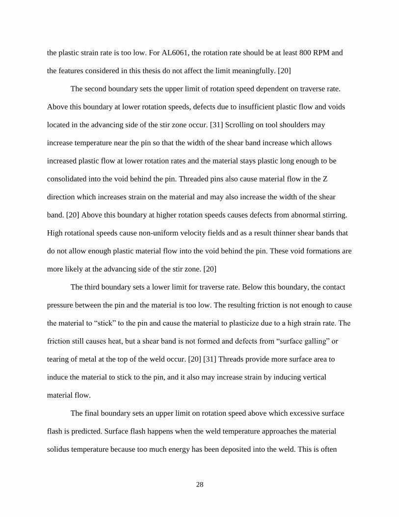
the plastic strain rate is too low. For AL6061, the rotation rate should be at least 800 RPM and

the features considered in this thesis do not affect the limit meaningfully. [20]

The second boundary sets the upper limit of rotation speed dependent on traverse rate.

Above this boundary at lower rotation speeds, defects due to insufficient plastic flow and voids

located in the advancing side of the stir zone occur. [31] Scrolling on tool shoulders may

increase temperature near the pin so that the width of the shear band increase which allows

increased plastic flow at lower rotation rates and the material stays plastic long enough to be

consolidated into the void behind the pin. Threaded pins also cause material flow in the Z

direction which increases strain on the material and may also increase the width of the shear

band. [20] Above this boundary at higher rotation speeds causes defects from abnormal stirring.

High rotational speeds cause non-uniform velocity fields and as a result thinner shear bands that

do not allow enough plastic material flow into the void behind the pin. These void formations are

more likely at the advancing side of the stir zone. [20]

The third boundary sets a lower limit for traverse rate. Below this boundary, the contact

pressure between the pin and the material is too low. The resulting friction is not enough to cause

the material to “stick” to the pin and cause the material to plasticize due to a high strain rate. The

friction still causes heat, but a shear band is not formed and defects from “surface galling” or

tearing of metal at the top of the weld occur. [20] [31] Threads provide more surface area to

induce the material to stick to the pin, and it also may increase strain by inducing vertical

material flow.

The final boundary sets an upper limit on rotation speed above which excessive surface

flash is predicted. Surface flash happens when the weld temperature approaches the material

solidus temperature because too much energy has been deposited into the weld. This is often

29

caused by too much axial force in the Z direction. [20] It has been shown that increasing traverse

rate can decrease the required axial load [32], but the amount that the traverse rate can be

increased is limited by the strength of the tool used. Shoulder scrolls may increase frictional

temperature and contribute to excessive flash occurring at lower rotational speeds.

5.2 Proposed Weld Parameter Metric

While this is a useful tool to compare different welds, it neglects the possibility of

different shoulder and pin sizes from different tools. This allows the possibility that two separate

welds with the same welding parameters could have drastically different results. A better way to

characterize welding parameters would be something that directly compares the thermal model to

the material model. While this method would couple the effects of changes in welding

parameters, it is not as straight forward. Its utility more than makes up for this weakness.

A proposed weld parameter matrix compares heat generation and flow band width. The

heat generation considers tool dimensions as well as rotation and transverse rates. Equation 5 is

used for the heat generation and assumes a sticking condition at the pin. The method described in

section 4 is used to find the flow band width. The proposed metric is shown in Figure 7.

30

Figure 7 - New Welding Parameter Map

As can be seen, there is a clear area where high strength welds appear. Furthermore, there

seems to be a trend that larger flow bands allow lower energy deposition, while smaller flow

bands tolerate more energy deposition. Figure 8 illustrates this trend by plotting the energy

deposition versus strength for groups of welds with the same shear band width. There are strong

relationships within the same shear band grouping between energy deposition and strength.

For welds with higher energy depositions, the material may experience melting, in which

case a different, non-solid-state joining phenomenon may be occurring. The process is still self-

regulating around a certain set of thermo-mechanical conditions, it is a question of where the

process is self-regulating from. Most models consider the material approaching a plastic state

from a solid state. The temperature is increased through both frictional and plastic dissipation

until the solidus temperature is reached, and viscosity decreases until material flows and

y = -0.001708x + 1.301538

0.6

0.7

0.8

0.9

1

1.1

1.2

1.3

0 200 400 600 800 1000 1200

Flo

w B

and

Wid

th (m

m)

Energy Deposition (J/mm)

<144 MPa

144-148 MPa

>148 MPa

Trendline

Linear (Trendline)

31

pressures on the material are released and the process repeats.

The process can also approach a plastic state from a liquid state, though. The plastic

material closest to the pin can begin to melt while plastic material towards the outside of the flow

band remains in a visco-plastic state. The melting of the material decreases the density and

resulting pressures resulting in an increase in the slip rate of the tool. The temperature then falls

to the solidus temperature because the temperature of material near the pin is dominated by

plastic dissipation and there is no plastic dissipation if slipping is dominant. Once the material

returns to a plastic state, a sticking condition occurs again and the process repeats. Higher

temperatures mean more phase changes and a lower weld strength if this micro-melting process

is occurring.

Crawford noted that a Couette Flow model correlated better than a visco-plastic flow

model weld pitches greater than 210 revolutions per inch. [2] This corresponds to about 8.33

revolutions per millimeter. Like before, this does not consider the dimensions of the tool and is

not a physical explanation. A weld pitch of about 8.33 revolutions per minute for his tool

corresponds to an energy deposition of about 750 Joules per millimeter using the tool dimensions

in Crawford’s experiment. Interestingly, this energy deposition limit is also present in traditional

arc welding when comparing arc length to weld width. It is explained in arc welding as the limit

where higher arc length increases heat distribution without significantly altering heat input. [3]

This phenomenon appears to occur at around 400 Joules per millimeter in the data given by Lim

et al. If the flow band graphs are then split into energy depositions roughly below and above 400

Joules per millimeter, precise relationships start to appear. These relationships are shown in

Figure 8.

32

Figure 8 - Energy Deposition vs Strength

So far, we have discussed optimal welding parameters and an upper limit on energy

deposition for a given flow band width. From the earlier discussion of flow bands, a lower limit

on energy deposition can be given below which flow bands will not form. This limit will be

different for every tool and welding set up but will be dependent on lowering viscosity below the

critical viscosity.

Using the experimental welding parameters, a yield strength of approximately 140 MPa

with no defects is predicted by first metric. It is relatively difficult to make this interpolation

given the metric. The proposed metric can give an equation for predicting strength. Since the

experimental welds in this thesis deposit much more than 750 J/mm, it is well within the Couette

Flow Model zone. Using calculations that will be developed in section 9.1 to verify the viscosity

model, the estimated flow band width is about 5 millimeters. Estimating a strength for Couette

130

135

140

145

150

155

160

0 200 400 600 800 1000 1200

Stre

ngt

h (M

Pa)


Flow Band 0.7-0.8 (VP)




Flow Band 0.7-0.8 (C)



Linear (FlowBand 1.0-1.1(VP))

33

Flow using an energy deposition of 2231 J/mm and a flow band width of 5 mm, the predicted

strength is lower than 135 MPa. The line is projected using only two data points, and such a

drastic energy deposition suggests the actual strength will be lower. More importantly, it

provides an intuitive way to evaluate how tool features could affect weld quality in the scope of

the models given above.

Figure 9 - Generalized Welding Parameter Map

y = -0.362ln(x) + 2.8271

0.6

0.7

0.8

0.9

1

1.1

1.2

1.3

0 200 400 600 800 1000 1200

Flo

w B

and

Wid

th (m

m)


<144 MPa

144-148 MPa

>148 MPa

Trendline

Log. (Trendline)

34

6. Tool Components

6.1 Shoulder

The shoulder generates frictional heat that is distributed into the weld and acts as a

preheating mechanism. It also contains plasticized material from the pin and consolidates it into

the weld. Shoulder diameter is typically three times the diameter of the pin. [5]

Early shoulder designs were concave that trapped escaping plasticized material until it

can be deposited into the void behind the weld. These tools required the tool to be tilted to allow

material into the concave shoulder shape. This required load to be applied in directions both

perpendicular and parallel to the weld direction to keep the tool from rising out of the material.

This requirement also limited the transverse speed. Finally, the tool tilt angle causes material

flow out of the material resulting in excess flash. [33]

The first attempts to make a convex shoulder were made by TWI, but they were

unsuccessful because the convex shape pushed material away from the welding zone. Scrolls

were eventually introduced and fixed this problem. Convex shoulders did not require a lead

angle because the outer edge of the shoulder did not contact the material allowing for rapid

changes in weld direction. It also provides more flexibility in weld height changes, so that the

amount of shoulder engagement does not affect weld quality as much and allowed for control by

varying shoulder engagement.

6.2 Pin

Pin heat generation is dominated by plastic dissipation and affects peak temperature near

the pin more than the distributed frictional heat generation by the shoulder. [5] Typical pin

diameters are the same as the thickness of plates to be welded. [5] The pin deforms and shears

material at the faying surfaces of the welded materials and the large strain rates, strains, and heat

35

generation plasticize the materials. Concurrently, the pin transports the material around the tool

and deposits it in the void. [33] This material is extruded between the pin and the parent material

on the retreating side. On the advancing side, the material can become entrained in a rotation

zone like a boundary layer and eventually flows into the void behind the pin in arc-shaped

features. [25]

Figure 10 - TWI Trivex tool (a) and MX-Trivex tool (b)

The most common shape for pins is a flat-bottom cylindrical pin because it is easy to

machine. Round-bottom pins can reduce tool wear upon plunging and improve the weld root

quality but are harder to machine. Truncated-cone pins have lower transverse loads and can be

used to weld thicker plates at faster speeds. Where threads are not possible in high-temperature

materials like ceramics, a stepped spiral profile can be used. TWI has developed a Whorl pin, the

Triflute pin, and the Trivex pin. The Whorl pin has a helical ridge on the pin surface like an

auger that directs material flow downward. This pin reduces the displacement volume by 60%

and reduces traverse loads. The Triflute pin contains three flutes cut into the helical ridge of the

Whorl and further reduces the displacement volume of the pin by 70% over the Whorl. The

Trivex pin has a triangular shape and reduced traverse forces by 18-25% and normal forces by

36

12% over the Triflute pin. [34] [35]

6.3 Material

The material of the pin can affect welding parameters in several minor ways. The

material of the tool must withstand maximum forces at welding temperatures. For welding at

lower temperatures, like the welds considered in this thesis, H-13 tool steel, Ferro-TiC SK, and

MP-159 can be used with maximum working temperatures around 550 degrees Celsius. For

higher temperature welds of steel or similar metals, Rhenium, Tungsten, and Polycrystalline

Cubic Boron Nitride tools are often considered because of their maximum work temperatures of

almost 2000 degrees Celsius. [2] [36]

37

7. Tool Component Features

7.1 Shoulder Scrolls

Shoulder scrolls pushed plasticized material from the outside of the shoulder back

towards the pin. This allows flat or convex tools to be used at reduced welding forces and

increase traverse speed without pushing all the material away from the weld zone or needing to

operate with a tool angle. [30] Scrolls also allow material displaced by the probe to escape

without being displaced as flash by directing it back toward the pin where it can eventually be

deposited back into the void left by the pin. [6] Shoulder scrolls also allow flat shoulders to be

used over concave shoulders and reduce welding forces required and increase traverse speed.

Scrolls have two suspected effects on material with respect to weld parameters. Scrolls

may increase the friction coefficient and resulting energy deposition. If there is no evidence of a

higher friction coefficient, this may suggest that a sticking condition occurs at the shoulder’s

surface. If there is a significant difference in weld strength between scrolled and non-scrolled

tools, this would confirm theories that scrolls improve material flow toward the pin and prevent

material from being pushed away.

7.2 Pin Threads

The main function of threads is to induce vertical material flow. [37] [2] [25] Threads do

not affect maximum temperature or temperature contours. [38] The threads are rotated in a

direction that drives material downward. As the material reaches the bottom of the material, it is

then forced away from the pin and then starts movement back upward toward the shoulder. This

induced vortex moves hot material away from the shoulder and may prevent material on top

from receiving too much energy. [12] [25] It also increases strain rate and strain on the material

near the pin, which may increase flow band width. This vortex may improve material flow to the

38

root of the weld, decreasing the likelihood of root or tunnel defects. It has also been observed

that the addition of threads reduces traverse forces. [2]

Threads may help decrease energy deposition for a set of welding parameters by

transporting hot material near the heat generation caused by the shoulder down into cooler

material. Weld strengths indicative of lower energy deposition would confirm this hypothesis. It

has also been suggested that increased material flow from threads can increase the strain rate and

the flow band width. Weld strengths proportional to flow bands widths could confirm this

hypothesis.

7.3 Triangular Pin

It was predicted that lower ratios between tool area and swept area would lead to lower

traverse force at a modest increase in required torque. The triangular pin required lower traverse

and axial forces. Interestingly, the threaded triangular pin required more traverse forces. [34]

[35] Triangular shaped pins may provide pockets for plasticized material to be regularly

distributed into the void behind the pin as the tool rotates. Since they are depositing plasticized

material three times per revolution as compared to once per revolution for circular pins, they are

maintaining a lower average pressure on the tool. This may account for lower traverse forces.

The triangular pin tool will be compared to the other tools in terms of weld strength,

traverse forces, and axial forces. Higher strength welds would suggest that material flow is

improved using triangular pins. The claims of decreased axial and traverse forces will be verified

or rejected.

39

8. Experimental Configuration

8.1 Machine Setup

Welds in this thesis were conducted at the Vanderbilt University Welding Automation

Laboratory with a Milwaukee #2K Universal Milling Machine that has been retrofitted with

motors and instrumentation to control spindle speed, transverse speed, lateral speed, and vertical

position. A Kistler dynamometer measures forces in x, y, and z directions, and torque. The

sensors and motors are connected to a Dell Precision 340 that uses MATLAB’s Simulink Real-

Time to generate a control signal that interfaces with a real-time target. The VUWAL FSW set

up is pictured in Figure 11.

Three butt welds of aluminum 6061-T6 were performed with each tool at a rotation rate

of 1400 RPM and a traverse rate of 152.4 mm/min. Plunge depths were iterated until

approximately 80% of the shoulder maintained engagement in the material. These values were in

the range of 5.4102 to 5.461 millimeters. The dimensions of the plates were approximately 406.4

x 76.2 x 6.35 millimeters. The nominal composition of aluminum 6061 is 1.0% Mg, 0.6% Si,

0.3% Cu, and 0.2% Cr.

40

Figure 11 - VUWAL FSW Machine [32]

8.2 Anvil Topography

This project began when it was noticed that weld quality during the second half of welds

was poor. Specifically, excessive flash increased as the weld progressed, and the tool was taking

too much material from the advancing side. Original hypotheses for the origin of these defects

were a loose or misaligned tool causing it to wobble, or the topography of our anvil was no

longer flat causing the tool to engage more material as the weld progressed.

To rule out a misaligned tool, the angle of the tool in relation to the anvil was examined

using levels and image processing . No misalignment was found. To examine the existence of a

tool wobble, a high-speed camera was used to record several welds looking down the traverse

41

axis. An image processing program was written to identify the tool from background noise, and

then track the position of the top and bottom of the tool. From this information, an angle was

determined and tracked throughout a weld. The max deflection of the tool was found to be about

0.5 degrees with a dominant frequency of 24.78 Hz. The tool was rotating at 1400 RPM, or 23.33

Hz. This was deemed most likely too small to affect weld quality.

Next, the topography of both the anvil and the specimen clamped onto the anvil were

mapped by lowering the tool until an axial force was detected by the dynamometer. The height

was recorded at various locations on the anvil alone and with specimen until a topography could

be interpolated. The topography of the anvil is shown in Figure 12.

Figure 12 - Anvil Topography

8.3 Specimen Topography

Next, the topography of the specimen clamped onto the anvil was mapped using the same

methods used to find the topography of the anvil. The specimen topography is shown in Figure

13.

42

Figure 13 - Specimen Topography

There is an obvious low spot on our anvil that translates to the specimen when it is

clamped to the anvil. This spot was most likely caused over years of FSW plunges all at

approximately the same location. It was estimated from past experimental observations that a

height change of around 0.005 inches could affect weld quality. The difference in height on the

specimen from the lowest point to the highest point is 0.0051 inches. While this difference could

start affecting welds, it should only affect welds at the highest point, or the extreme end of the

weld, and then only slightly. Excessive flash in previous welds began to become a problem

around halfway through the weld, or at about 20 inches in the traverse direction on the figure. To

rule out weld topography, a weld in the opposite direction was conducted. Severe flash was still

reported, though it was noticed earlier in the weld.

8.4 Tools

Four different tool designs were used in this thesis. All tools were manufactured of H-13

steel heat treated to Rc 48-50, had one inch (25.4mm) diameters, shoulder angles of 7 degrees,

0.25 inch (6.35 mm) pin diameters, and 0.185 inch (4.699 mm) pin height. The first tool had a

43

round, threaded pin and a scrolled shoulder. The second pin had a round, threaded pin but no

scrolled shoulder. The third pin had a scrolled shoulder but no threads on the circular pin. The

final tool had a threaded pin, scrolled shoulder, and a triangular shaped pin. The tools are

pictured in Figure 14 from left to right: TPS 9545, TP 9545, PS 9545, TPS 9545_t.

Figure 14 - Tools used in experiments (TPS 9545, TP 9545, PS 9545, TPS 9545_t)

8.5 Weld Data

A Kistler Rotating quartz four-Component Dynamometer (RCD) measured forces and

torque on the tool. The output voltages of the dynamometer were digitized and transmitted to a

stator connected to a computer. The stator was rigidly, concentrically mounted 2 mm away from

the RCD.

A custom C# package is used for data collection. This package records the output data

from the dynamometer and outputs a CSV text file. This data is then imported into MATLAB for

post processing.

8.6 Optical Testing Methods

Several optical methods were attempted in analyzing and testing the welds. Videos were

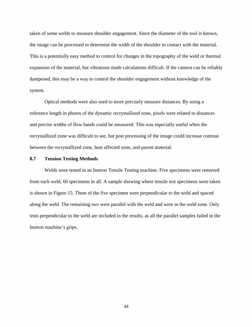
44

taken of some welds to measure shoulder engagement. Since the diameter of the tool is known,

the image can be processed to determine the width of the shoulder in contact with the material.

This is a potentially easy method to control for changes in the topography of the weld or thermal

expansion of the material, but vibrations made calculations difficult. If the camera can be reliably

dampened, this may be a way to control the shoulder engagement without knowledge of the

system.

Optical methods were also used to more precisely measure distances. By using a

reference length in photos of the dynamic recrystallized zone, pixels were related to distances

and precise widths of flow bands could be measured. This was especially useful when the

recrystallized zone was difficult to see, but post processing of the image could increase contrast

between the recrystallized zone, heat affected zone, and parent material.

8.7 Tension Testing Methods

Welds were tested in an Instron Tensile Testing machine. Five specimens were removed

from each weld, 60 specimens in all. A sample showing where tensile test specimens were taken

is shown in Figure 15. Three of the five specimen were perpendicular to the weld and spaced

along the weld. The remaining two were parallel with the weld and were in the weld zone. Only

tests perpendicular to the weld are included in the results, as all the parallel samples failed in the

Instron machine’s grips.

45

Figure 15 - Sample showing locations of tensile test specimen

46

9. Results

9.1 Flow Band Model Verification

To the author’s knowledge, there has never been a test of the critical viscosity theory

proposed by Nandan et al. To verify the Nandan model, three welds were completed with

rotation rates ranging from 1200 to 1600 RPM and a fixed transverse rate of 254 mm/min, and

three welds were completed with a fixed rotation rate of 1400 RPM and transverse rates ranging

from 101.6 to 203.2 mm/min. Table 1 summarizes the weld parameters and resulting flow band

widths for the verification welds.

Table 1 - Verification Weld Parameters and Results

The pin was stopped and quenched after steady state conditions were met. Specimens

were then taken just behind the keyhole left by the pin in the material. These specimens were

water-sanded, polished, and etched with Kellers reagent. The resulting etch of the weld was

analyzed to determine the width of the flow band. The measured flow band width was found by

measuring the width of the recrystallized zone caused by the pin through the center of the area

(shown by white arrows on images). The thickness of the specimen is known to be 6.35 mm and

is used as a reference distance to convert the pixel width to a width in millimeters. The resulting

width in millimeters is then divided by two because the flow band is theoretically symmetrically

created on both sides of the pin. The etches of the six verification welds filtered using

MATLAB’s ADAPTHISTEQ filter are shown in Figure 16.

Name Rotation Rate (RPM) Transverse Rate (mm/min) Measured Flow Band Width (mm) Predicted Flow Band Width (mm) Error

Verification Weld 1 1200 254 4.23 4.79 13.13%



Verification Weld 4 1400 101.6 5.31 5.20 2.10%



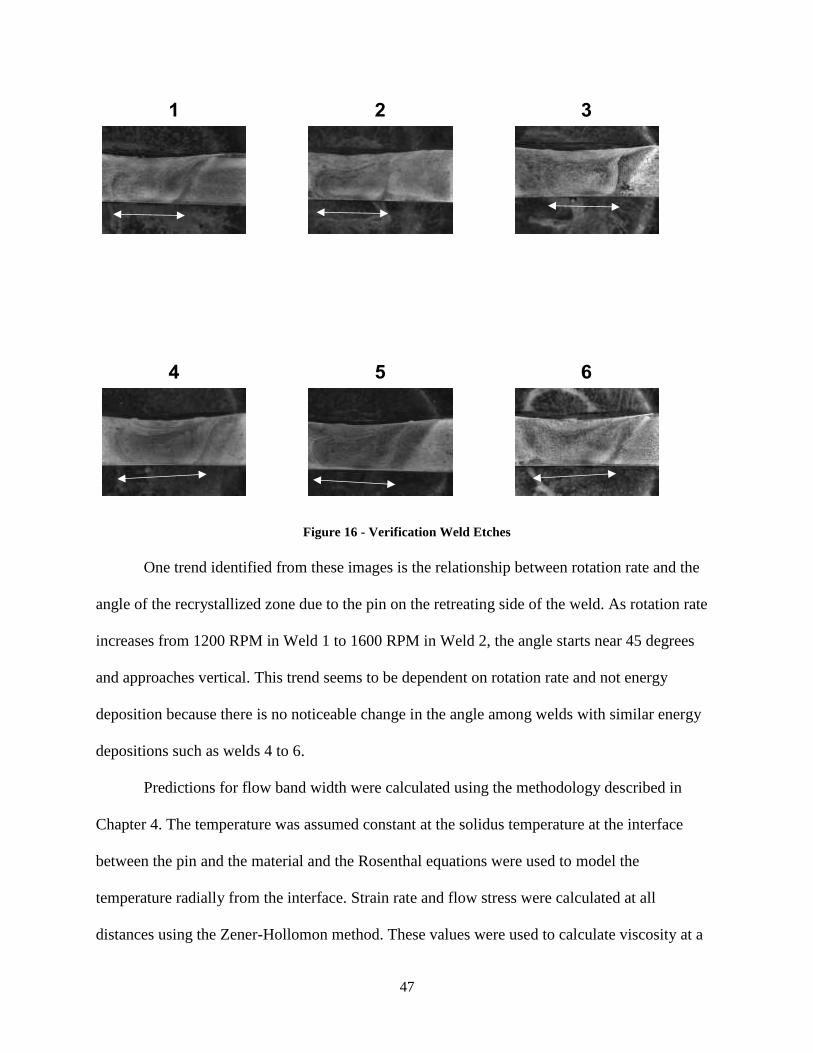
47

Figure 16 - Verification Weld Etches

One trend identified from these images is the relationship between rotation rate and the

angle of the recrystallized zone due to the pin on the retreating side of the weld. As rotation rate

increases from 1200 RPM in Weld 1 to 1600 RPM in Weld 2, the angle starts near 45 degrees

and approaches vertical. This trend seems to be dependent on rotation rate and not energy

deposition because there is no noticeable change in the angle among welds with similar energy

depositions such as welds 4 to 6.

Predictions for flow band width were calculated using the methodology described in

Chapter 4. The temperature was assumed constant at the solidus temperature at the interface

between the pin and the material and the Rosenthal equations were used to model the

temperature radially from the interface. Strain rate and flow stress were calculated at all

distances using the Zener-Hollomon method. These values were used to calculate viscosity at a

48

range of distances from the pin until the critical viscosity was exceeded. The results are

summarized in Table 1.

Figure 17 - Flow Band Width Calculations

The resulting flow band width model dependent on critical viscosity is highly dependent

on energy deposition. Figure 20 demonstrates this relationship. The three tightly grouped data

points in the lower left section of the graph have a fixed transverse rate, and rotation rates

ranging from 1200 to 1600 RPM. The three data points that are more dispersed have fixed

rotation rates with traverse rates ranging from roughly 100 to 200 mm/min. There are not enough

data points to make any firm observations, but it appears that higher rotation rates will eventually

result in less increase in flow band widths but reducing traverse rates will linearly increase the

flow band width. The energy deposition is dependent on the tool dimensions, rotation rate, and

transverse rate. The relationship for both the rotation rate and the transverse rate with the flow

band width is described in Figure 19 and Figure 20. Linear relationships with slopes similar to

the trendlines shown but with shifted y-intercepts are predicted for data where only one data

49

point is shown.

Figure 18 - Verification Welds Rotation Rate vs Flow Band Width

y = 0.000353x + 3.821617R² = 0.901056

4

4.2

4.4

4.6

4.8

5

5.2

5.4

1100 1200 1300 1400 1500 1600 1700

Flo

w B

an

d W

idth

(m

m)

Rotation Rate (RPM)

TR=254 TR=101.6 TR=152.4 TR=203.2 Linear (TR=254)

50

Figure 19 - Verification Welds Rotation Rate vs Flow Band Width

y = -0.006155x + 5.924070R² = 0.988586

4

4.2

4.4

4.6

4.8

5

5.2

5.4

50 100 150 200 250 300

Ba

nd

Wid

th (m

m)

Transverse Rate (mm/min)

RPM=1400

RPM=1200

RPM=1600

Linear (RPM=1400)

51

Figure 20 - Energy Deposition vs Flow Band Width

Error between predicted flow band widths and measured flow band widths for

verification welds ranged from 1% to 13%. Error was discovered to be largely influenced by the

weld’s energy deposition. Lower energy depositions resulted in higher error for the prediction.

This error split is between welds with more or less than 1600 J/mm energy deposition and is

depicted graphically in Figure 21.

y = 0.000498x + 3.718123

R² = 0.928266

4

4.2

4.4

4.6

4.8

5

5.2

5.4

5.6

1000 1500 2000 2500 3000 3500

Flo

w B

an

d W

eld

(m

m)


52

Figure 21 - Flow Band Prediction Error vs Energy Deposition

Etches were also made of specimens from welds using the tools TP 95.45, PS 95.45, and

TPS 95.45. These specimens were analyzed to determine the impact of tool parameters on the

flow of material in the weld. Table 2 demonstrates that both threads and scrolls have an impact

on increasing flow band width, though threads have a much larger impact.

Table 2 - Flow Band Width by Tool Feature

9.2 Axial Force

Several trends or observations that span entire welds will be made here, but this data will

later be localized to the area where each specimen was taken to find the mechanical conditions

y = 4E-06x + 0.0046

R² = 0.5177

y = -0.0003x + 0.4663R² = 0.9874

0.00%

2.00%

4.00%

6.00%

8.00%

10.00%

12.00%

14.00%

0 500 1000 1500 2000 2500 3000 3500 4000

Erro

r


Error vs Energy Deposition

More than 1600 J/mm

Less than 1600 J/mm

Linear (More than 1600 J/mm)

Linear (Less than 1600 J/mm)

Name Rotation Rate (RPM) Transverse Rate (mm/min) Measured Flow Band Width (mm) Predicted Flow Band Width (mm) Error

PS Sample 1400 152.4 3.81 4.99 30.89%

TP Sample 1400 152.4 4.44 4.99 12.36%

TPS Sample 1400 152.4 4.49 4.99 11.06%

53

that contributed to the specimen’s strength. Three key observations can be made about the axial

force measurements. The first is the rank of the magnitude of the axial forces between the tools.

The TPS-t tool has axial force results on the order of half of the values for other tools, ranging

from as low as 4000 N to 12,000 N. The TPS-t tool also sees the largest increase in axial force

between individual welds. The PS tool ranges from 6000 to 14,000 N with weld three differing

greatly from the first two. The TP tool ranged from 8000 to 12,000 N. Finally, the TPS tool had

the largest axial forces, ranging from 10,000 N to 17,000 N.

Figure 22 - Raw Axial Force Weld Data

Most welds exhibit an increase in axial force over the course of the weld. This has been

attributed to thermal expansion of the material earlier in this thesis. Weld 1 using the TP tool was

purposely welded at a location that utilized the low point of the anvil’s topography to examine

the effect this may have on weld quality. The dip in the anvil topography occurs at about 10

inches for reference in Figure 22. The increase in axial force across most individual welds is

approximately 2000 N, but some of this can also be attributed to rising anvil topography.

54

It is obvious from the force data that the pin broke off around a transverse location of 19

inches on the third weld for TPS 9545_t. The axial forces during the second weld were nearly

double the first weld which may have contributed to the pin breaking. The force data for the third

weld has a discontinuity increase from about 6000 N to 8000 N, but otherwise seems unaffected

by the event. The process seems to attempt to self-regulate with the new circumstances of the

weld. It is unknown but interesting why an absence of a pin would increase the axial force.

The final observation concerns the magnitude of periodic axial force oscillations between

the tools. Again, the TPS-t tool exhibited behavior drastically less than the other tools, at no

more than 1000 N oscillations. The TP tool exhibited oscillations roughly 2000 N in magnitude.

The PS and TPS tools both exhibited oscillations roughly 4000 N in magnitude.

Interestingly, when the axial force at the specimen locations is compared with the

specimen yield strength, there are clear areas that each tool exists in that become even clearer in

measurements below. The TP 9545 tool generally experiences more axial force at about 12,000

N, the TPS tool experiences about 10,000 N, and the TPS9545_t tool experiences the least at a

range from 5000-9000 N. The PS 9545 tool is very nonuniform with axial forces ranging from

7000-12,000 N. There does not appear to be an optimal value for axial force concerning resulting

yield strength.

55

Figure 23 - Axial Force at Specimen Locations

9.3 Transverse Force

Forces are measured with an axis rotating with the tool. The transverse force can be

calculated using both the rotating x and y force measurements, but oscillations at various

frequencies make the results questionable. The measured magnitude should be at a maximum

value when the measured force in the x direction lines up with the stationary axis of the moving

table and at an equally negative value when the axis is 180 degrees out of phase. The maximum

and minimum values averaged over every 100 data points is shown in Figure 24. The maximum

magnitudes were used for transverse forces exhibited at the specimen locations. The magnitudes

of the maximum and minimum values are not equal, and the magnitude of the minimum value is

usually greater. This could be caused by a slight misalignment of the tool in relation to the anvil

or descriptive of the material sticking to the tool for part of the rotation.

80

90

100

110

120

130

140

150

160

170

4000 6000 8000 10000 12000 14000 16000

Yiel

d S

tren

gth

(MP

a)

Axial Force (N)

Axial Force vs Yield Strength

PS9545

TPS9545

TP9545

TPS9545t

56

Figure 24 - Transverse Force Minima and Maxima

Transverse forces are much more constant across the length of a weld, from one weld to

another, and across different tools. Both TPS 9545 and PS9545 exhibit transverse forces around

1500 N, while TP 9545 only exhibits transverse forces around 1000 N. Scrolls appear to increase

the required transverse force by 500 N. The triangular pin tool exhibits much lower forces than

the circular tools. The first two welds oscillated between about 250 N to -600 N, displaying a

much more pronounced asymmetry than the other tools as well. The pin breaking is very evident

in the third weld, and an unexpected transient behavior is displayed after this event. During the

second weld, at about the 18 inch location the transverse force data becomes more erratic

signaling the initial weakening of the joint between the pin and the shoulder. It appears an

internal fracture occurred in the pin during the second weld, but the pin did not actually break off

until the third weld.

When the transverse forces at the specimen locations are examined there is a similar

grouping of tool values found as was noticed in axial forces at specimen locations. The PS 9545

and TPS 9545 tools demonstrate the largest magnitude of transverse forces ranging from 1100 to

57

1600 N and 1500 to 2000 N respectively. The TP 9545 and TPS 9545_t transverse forces

demonstrate much lower magnitudes at 700 to 1100 N and 150 to 350 N respectively.

Figure 25 - Transverse Force at Specimen Locations

9.4 Torque

Torque across an entire weld varied slightly between circular pins and drastically for the

triangular pin. The TP 9545 tool exhibited the least maximum torque at 20 N-m, followed by PS

9545 at 30 N-m, and finally TPS 9545 at 35 to 40 N-m. The triangular pin exhibited much lower

maximum torques at around 11.5 N-m, with the effects of the pin breaking off very apparent.

80

90

100

110

120

130

140

150

160

170

0 500 1000 1500 2000 2500

Yiel

d S

tren

gth

(MP

a)

Transverse Force (N)

Transverse Force vs Yield Strength

PS9545

TPS9545

TP9545

TPS9545t

58

Figure 26 - Torque Minima and Maxima

The torque oscillates between two torque values, and the maximum torque value is

potentially the more interesting value. The tool applies torque until the material yields while the

material is sticking to the tool. The tool then either slips or the viscosity of the material decreases

until it is plastic enough to flow. The maximum torque would be the torque applied to achieve

the flow stress of the material. The torque for PS 9545 is 25 to 32 N-m, TP 9545 is around 16 to

22 N-m, TPS 9545 is erratic varying from 28 to 41 N-m. The first weld for the triangular tool has

a uniform maximum torque around 11.5 N-m, the lowest of all the tools, and the lowest

difference between maximum and minimum torque values. The second weld displays similar

behavior to the first weld until about the 18 inch mark and then shows increasing magnitudes of

oscillation. The third weld demonstrates torque values similar to the first weld until about the 19

inch mark when the pin obviously breaks and the torque magnitude of oscillation and maximum

torque values greatly reduce to negligible values.

The strongest relationship between in-process measurements and resulting yield strength

occurs for torque. There is an inversely proportional relationship between torque and yield

59

strength. As torque increases, yield strength decreases. The values in Figure 27 are the maximum

torque values where the specimen was taken. The tools exhibit distinct, vertical bands of torque

values. The triangular tool exhibits the widest range of torque values from 0 to 12 N-m, but only

because of the pin breaking. If the third weld’s values are discounted, the triangular tool has the

most uniform values at 11.5 with a standard deviation of only 0.27 N-m. The TPS tool from 31

to 36 N-m, the PS tool from 26 to 29 N-m, and the TP tool from 16 to 20 N-m.

Figure 27 - Torque at Specimen Locations

9.5 Yield Strength

Yield strengths were calculated using the 0.2% offset method and the following figures

show each weld’s stress-strain curve and associated offset intersect line. The moduli are

generally similar among the same welds and across different welds with the same tool. This

80

90

100

110

120

130

140

150

160

170

0 5 10 15 20 25 30 35 40

Yiel

d S

tren

gth

(MP

a)

Torque (N-m)

Torque vs Yield Strength

PS9545

TPS9545

TP9545

TPS9545t

60

demonstrates that the data is acceptable overall and is a factor for excluding outliers when this is

not true. For example, in weld 2 of Figure 29 the center specimen (TP 9545_2VC) is much

greater than the strengths of all other specimen for the same tool. This data was excluded as an

outlier for many reasons including the large difference in this specimen’s modulus. The left

specimen in Figure 30 (TPS 9545_5VL) was also excluded as a low outlier for the same reasons.

The final weld for the triangular tool (TPS 9545_t_3VC, TPS 9545_t_3VL, TPS 9545_t_3VR)

was also excluded because a successful weld was not achieved after the pin broke.

It is likely that the erroneous data occurred during tensile testing. Our samples were three

inches in width, and the extensometer used was a little over one inch wide. This did not leave

much material for the grips to affix to. This lead to some specimens failing at the grip interfaces

instead of in the material. Future specimens should be wider to avoid this issue.

Figure 28 - PS 9545 Tensile Test Results

61

Figure 29 - TP 9545 Tensile Test Results

Figure 30 - TPS 9545 Tensile Test Results

62

Figure 31 - TPS 9545-t Tensile Test Results

A summary of moduli, strengths, and mechanical conditions for all specimens is shown

in Table 3. The welds are color coded according to the number weld they were in a session of

welding to account for thermal affects that might occur if the tool and anvil had not returned to

room temperature. For example, all the TPS 9545 welds were conducted in one day during a

single session but required two test welds were performed to test weld parameters. The two test

welds were weld numbers one and two of the session, and the first official weld was the third

weld of the session. No significant trends could be identified with the small amount of data

associated with weld number.

63

Table 3 - Raw Specimen Test Data

Table 4 shows a simple analysis of the average yield strength, standard deviation, and

Weld Weld Modulus Ultimate Strength Yield Strength Torque Break Z Force Break X Force Break

Name # Mpa Mpa Mpa N-m N N

PS9545_1VC 1 96869 200.9180 120.0135 28.1118 12695.3125 1601.0465 First Weld

PS9545_1VL 1 66235 179.4390 95.2783 27.2404 12041.0156 1566.1709 2nd Weld

PS9545_1VR 1 48103 187.2970 126.9649 28.1118 9951.1719 1383.8358 3rd+ Weld

PS9545_2VC 1 56944 193.5480 132.1117 29.1246 13144.5313 1504.8968

PS9545_2VL 1 56922 203.0960 139.0914 27.1740 13095.7031 1266.8647

PS9545_2VR 1 54326 139.7240 123.2600 29.1246 11113.2813 1411.6471

PS9545_3VC 1 44010 202.5940 124.3726 25.8236 9990.2344 1311.7792

PS9545_3VL 1 50928 199.4870 131.4096 27.7598 9365.2344 1130.6339

PS9545_3VR 1 49084 180.8730 113.3501 25.8236 8115.2344 1157.0323

Averages 58157.89 187.44 122.87 27.59 11056.86 1370.43

Standard Dev 14971.62 18.92 12.02 1.15 1701.19 159.40

TPS9545_3VC 3 65150 196.0200 136.1708 34.9966 14218.7500 1812.8289

TPS9545_3VL 3 66512 211.9330 156.9472 31.3003 13310.5469 1476.6393

TPS9545_3VR 3 64038 212.2550 122.2392 34.9966 12373.0469 1478.7958

TPS9545_4VC 4 49324 193.4930 123.3241 31.8572 14130.8594 1776.2429

TPS9545_4VL 4 51409 185.6680 115.5980 31.8196 13544.9219 1535.1620

TPS9545_4VR 4 53030 161.9330 127.0627 31.8572 12646.4844 1566.3196

TPS9545_5VC 5 40749 174.4670 103.5525 35.3399 15332.0313 1939.3183

TPS9545_5VL 5 26265 151.6190 90.5838 36.1911 15322.2656 1608.1109

TPS9545_5VR 5 63291 188.6300 117.7268 35.3399 13769.5313 1730.5104

Totals 56687.88 190.55 125.33 33.74 13849.83 1658.21

Standard Dev 8769.75 16.09 14.83 1.74 877.51 162.22

TP9545_1VC 3 63332 217.6280 134.9175 17.7933 10634.7656 742.0935

TP9545_1VL 3 62236 213.9510 128.6961 16.0938 10263.6719 755.6273

TP9545_1VR 3 57517 197.0040 131.8038 17.7933 10263.6719 1105.8714

TP9545_2VC 1 149091 237.2270 227.38949 19.7554 12363.2813 981.1667

TP9545_2VL 1 63135 218.6080 127.7060 19.6169 11650.3906 779.0513

TP9545_2VR 1 38259 202.7650 147.7157 19.7554 10039.0625 687.7350

TP9545_3VC 2 49137 225.7360 148.5296 20.1623 12128.9063 1067.2776

TP9545_3VL 2 84334 225.6100 140.8387 18.0184 11259.7656 818.7605

TP9545_3VR 2 70003 215.8910 142.8207 20.1623 9843.7500 721.2722

Totals 60994.13 214.65 137.88 18.79 10938.59 850.98

Standard Dev 12782.16 9.50 7.72 1.38 773.31 150.11

TPS9545_t_1VL 3 62747 208.8770 137.3196 11.9964 5878.9063 261.4189

TPS9545_t_1VC 3 53915 204.6270 135.1026 11.5203 5341.7969 237.9206

TPS9545_t_1VR 3 51494 195.0510 132.6896 11.9964 5029.2969 215.0171

TPS9545_t_2VC 1 55737 200.7890 140.4433 11.3818 10283.2031 291.0892

TPS9545_t_2VL 1 45572 197.5390 136.5379 11.8175 9140.6250 347.4555

TPS9545_t_2VR 1 57838 198.5140 131.2975 11.3818 7587.8906 134.6320

TPS9545_t_3VC 2 35156 65.9990 63.8153 0.1861 8486.3281 269.0781

TPS9545_t_3VL 2 23746 65.1160 61.5101 4.3556 6250.0000 -162.2946

TPS9545_t_3VR 2 0.1861 5585.9375 -145.2658

Totals 54550.50 200.90 135.57 11.68 7210.29 247.92

Standard Dev 5319.11 4.63 3.01 0.27 1971.98 65.79

64

coefficient of variance across all tools. The TP 9545 tool resulted in the highest average strength,

the TPS 9545 tool exhibited the largest standard deviation, and the TPS 9545_t tool exhibited the

lowest standard deviation. Coefficients of variance ranged from just over 2% for the TPS_9545_t

tool to almost 12% for the TPS 9545 tool.

Table 4 - Tool Result Analysis

Finally, Table 5 attempts to describe any effect of anvil topography on the strength of

welds across all tools. Overall, specimens taken from the right side (near the beginning) of the

weld were weaker by 1-2 MPa. This trend was stronger for the TPS 9545 and TPS 9545_t tools,

while the TP 9545 demonstrated stronger than average strengths on the right. The strongest

location for all tools but TPS 9545 was in the center, but the strongest location across all tools

was the left side.

Table 5 - Specimen Location Result Analysis

The relationship between location of specimen and strength may be better characterized

by Table 6. The mean strengths at each location were divided by the overall mean strength for

AVG PS St Dev Coef of Var AVG TPS St Dev Coef of Var AVG TP St Dev Coef of Var AVG TPS_t St Dev Coef of Var

122.87 12.02 9.78% 125.33 14.83 11.84% 137.88 7.72 5.60% 135.57 3.01 2.22%

Mean Left St Dev Coef of Var Mean Center St Dev Coef of Var Mean Right St Dev Coef of Var

Overall

130.72 15.53 11.88% 130.08 12.03 9.25% 128.81 10.10 7.84%

PS 9545

121.93 19.10 15.67% 125.50 5.00 3.99% 121.19 5.75 4.74%

TPS 9545

136.27 20.67 15.17% 121.02 13.42 11.09% 122.34 3.81 3.12%

TP 9545

132.41 5.97 4.51% 141.72 6.81 4.80% 140.78 6.65 4.73%

TPS 9545_t

135.82 0.72 0.53% 138.88 1.56 1.12% 131.99 0.70 0.53%

65

each tool. This allows better comparisons between different tools. This table makes it apparent

that the TP 9545 exhibits a unique trend from all other tools.

Table 6 - Percentage of Mean Strength by Specimen Location

Left Center Right

Overall 100.68% 100.19% 99.21%

PS 9545 99.23% 102.14% 98.63%

TPS 9545 108.73% 96.56% 97.62%

TP 9545 96.04% 102.79% 102.10%

TPS 9545_t 100.19% 102.45% 97.37%

66

10. Discussion

10.1 Tool Features Effect on Transverse Force

The standard tool for comparisons will be the TPS 9545. The threadless PS 9545 tool

exhibited transverse forces almost 300 N less than the standard tool with a standard deviation

almost identical to the standard tool. The threads increase strain rate by creating vertical flow.

This could decrease viscosity of the material slightly and consequently decrease transverse

forces. This vertical flow is eventually impeded by the anvil and forced horizontally. This

horizontal flow seems to dominate the decrease in viscosity created and result in an increase in

transverse forces when using threads. The almost identical standard deviation to the standard tool

signals that threads do not contribute to orderly flow in the plasticized region.

The TP 9545 tool without scrolls exhibited transverse forces more than 800 N less than

the standard tool with a standard deviation less than the standard tool. This demonstrates that

scrolls play a large part in increased transverse forces. The scrolls direct colder material at the

outside of the weld zone towards the pin to be strained and warmed to lower viscosity. This

increases the flow band zone and affects the dynamic recrystallized zone shape which will be

further discussed in a later section. The cost of driving this colder material towards the pin is

increased transverse forces, which is demonstrated by these results.

The triangular pin tool exhibited transverse forces over 1500 N less than the standard tool

with a standard deviation much less than the standard tool. Flow past a confined rotating circular

cylinder is prone to vortex shedding which creates fluctuating pressures in the cylinder’s wake.

[39] The high rotation rate and low Reynolds number tend to reduce vortex shedding and

increase Magnus effect forces which also affects flow behind the pin. Though vortex shedding

may not occur under FSW conditions, the inhibition of boundary layer separation has been

67

shown. [40] This explains the recirculation of material around the pin. Turbulence could result

from vortex shedding or the outer layer of recirculated material interacting with stationary parent

material. This turbulence combined with oscillations between sticking and slipping could

contribute to turbulent mechanical conditions behind the pin and high standard deviations

resulting in strength. In contrast, a triangular pin separates plasticized material into orderly

packets with smaller vortices and smaller pressure fluctuations in its wake. This lack of

turbulence could translate to lower standard deviation in transverse forces for triangular pin

tools.

10.2 Tool Features Effect on Axial Force

The threadless PS 9545 tool exhibits axial forces almost 3000 N less than the standard

tool at a standard deviation almost twice that of the standard tool. The decrease in axial forces is

expected since threads drive material downward and increase axial forces. The threads also

create more predictable vertical flow, causing less variance in axial force.

The unscrolled TP 9545 tool exhibits axial forces almost 300 N less than the standard

tool at a standard deviation more than 100 N less than the standard tool. The scrolls direct

material back towards the pin which results in increased axial forces, but the results show that

this effect is not anywhere near the effect that pins have on axial force. The unscrolled tool

allows material to escape the shoulder which slightly reduces axial forces.

The triangular pin TPS 9545_t tool exhibits axial forces more than 6500 N less than the

standard tool at a standard deviation over 1000 N more than the standard tool. The values for the

first weld alone, discounting the second weld that had a weakening pin, displays axial forces

more than 8000 N less than the standard tool and a standard deviation more than 500 N less than

the standard tool. The weakening pin obviously contributed to fluctuating axial forces, but if the

68

data from the first weld alone is used the TPS 9545_t tool has drastic reductions in magnitude

and oscillations of axial forces. Like with the transverse forces, this may be a result of laminar

flow because vortexes are not formed as with the circular pin. This explains why both the

magnitude and the standard deviation of axial forces is much lower.

10.3 Tool Features Effect on Torque

The threadless PS 9545 tool exhibited torques more than 6 N-m less than the standard

tool and a standard deviation more than 0.5 N-m less than the standard tool. The torque is likely

heavily influenced by the axial force, but this does not entirely account for torque values. The PS

9545 and TP 9545 tools had similar axial force values but differ greatly in torque values. While

the PS 9545 tool had the greatest standard deviation for axial force, only the triangular tool has a

smaller standard deviation for torque. The threads induce vertical flow and vertical strain which

can reduce viscosity. The reduced viscosity means more material is plasticized and rotated with

the tool. This increased material requires more torque for the tool to rotate. Since there is less

plasticized material without a threaded tool, the amount of plasticized material varies less and

results in a smaller standard deviation for torque.

The unscrolled TP 9545 tool exhibited torques almost 15 N-m less than the standard tool

and a standard deviation almost 0.5 N-m less than the standard tool. Scrolls direct denser

material back toward the pin requiring torque to rotate it. Without the scrolls, material is allowed

to escape which greatly reduces torque required by the machine. The parameters used in this

experiment likely produce too much plasticized material, so allowing material to escape is

beneficial at these conditions. If the heat input is reduced, an unscrolled tool may allow too much

material to escape and fail to be consolidated behind the pin.

The triangular TPS 9545_t tool exhibited torques more than 22 N-m less than the

69

standard tool and a standard deviation about 15% of the standard tool. This is likely a

compounding effect of both lower axial and transverse forces achieved through more laminar

flow when compared to circular pins.

10.4 Tool Features Effect on Yield Strength

The threadless PS 9545 tool had the lowest yield strength of all the tools. This

demonstrates the importance of threads to effective material flow. Without threads to drive the

material downward, excess material accumulates at the top of the weld and is expelled as flash.

[38] This tool also had higher standard deviations for in process forces and yield strength

suggesting a correlation between turbulent flow and resulting weld strength. Interestingly, it had

a low standard deviation for torque. Torque magnitude may be a slight indication of weld

strength, though oscillations in weld magnitude do not seem to affect the process greatly.

The unscrolled TP 9545 tool demonstrated the highest yield strength of all the tools. This

result may be an outlier due to the welding parameters used for this experiment. In comparison

with welding parameters of similar experiments, this experiment had higher rotation rates

resulting in higher heat input. The TP 9545 tool does not direct excess material back towards the

pin. This tool may not direct enough material back to the pin to be reconsolidated for lower heat

input experiments. Excessive flash was observed with the PS 9545 tool suggesting that allowing

some material to escape under these conditions is beneficial for flash reduction.

The triangular pin TPS 9545_t tool demonstrated strengths comparable to the TP 9545

tool at 135.57 MPa compared to 137.88 MPa respectively. The standard deviation of strengths

for the triangular tool was also less than 40% of the TP 9545 tool results. This follows the trends

from the earlier observations of in-process force oscillations causing more predictable, laminar

flow.

70

The overall strengths of the welds are far below what a traditional welding parameter

metric may predict. As was mentioned in section 5, the predicted weld strength using this

experiment’s parameters was about 140 MPa. Actual strengths range only from 122 to almost

138 MPa, and only 125 MPa for the standard tool. This was predicted by the proposed welding

parameter metric in section 5. This lower strength may be a result of the material acting more

like a liquid under such high heat input conditions. The temperature graph in Figure 17 also

supports this idea. The temperature was held at the solidus temperature if the calculated

temperature was greater than the solidus temperature. The graph demonstrates that the

temperature is greater than the solidus temperature for a large portion of the flow band and may

contribute to melting or phase changes in this region. Welding parameters should optimize the

heat input to minimize this high temperature region of the weld zone. This explanation matches

with previous conclusions by Crawford et al. and explains the observations of excess flash

noticed using tool PS 9545. Tool TP 9545 may avoid excess flash by not drawing already heated

material into the weld zone to be reheated to excess temperatures.

10.5 Tool Features Effect on Dynamic Recrystallized Zone Shape

Figure 32 shows the etches of the weld zone for all tools except TPS 9545_t. No etching

was done for the TPS 9545_t tool because a suitable sample could not be made. This was an

oversight and future work should cover the shape of the weld zone for a triangular pin. The heat

affected zones, shown in dark gray, are similar for all welds. This is expected because this area is

thought to be mainly influenced by the heat from the shoulder’s rotation, and rotation rates for all

specimen were the same. The right side of the dynamic recrystallized zone (DXZ), shown in the

lighter gray inside the heat affected zone, all seem similar as well. The key differences between

all samples is found in the shape of the left (retreating) side of the DXZ.

71

Figure 32 - Etches of Welds from Different Tools

The DXZ of the PS 9545 sample has an angle of about 45 degrees until halfway down to

the root of the weld where a small vertical section is observed. This suggests that shoulder

effects dominate the shape of the DXZ for this tool. This is expected since there are no threads to

influence flow from the pin. The result is a much narrower DXZ. Since the DXZ is not the

weakest part of the weld, a smaller cross-sectional area DXZ correlates to lower weld strength.

The DXZ of the TP 9545 sample is almost vertical and recedes near the top of the weld

near the shoulder. There is no indication of any effect from the shoulder in the DXZ. This wider

cross-sectional area of DXZ may correlate to the TP 9545 tool’s higher yield strengths, but it

cannot be the sole reason because it was not the only tool with threads on the pin.

The DXZ for the standard TPS 9545 tool has a shape similar to the PS 9545 tool, but not

as narrow. The angle changes to be more vertical in about the top quarter of the weld, resulting in

more cross-sectional area for the DXZ. The cross section is similar to, if not greater than the

72

cross-sectional area for the TP 9545 tool. It is hypothesized that the lack of scrolls actually

benefitted the TP 9545 tool by not drawing in excess, overheated material to be consolidated into

the weld or expelled as flash. The TPS 9545 tool may produce superior welds if the welding

parameters lower heat input. Future work should be completed to confirm this hypothesis.

10.6 Tool Features Effect on Flow Band Width

Table 2 shows the comparison of the predicted flow band widths at the experimental

welding parameters and the measured flow band widths for all tools except TPS 9545_t. These

results confirm the observations made about the shape of the DXZ that the PS 9545 tool has the

smallest flow band width, followed by TP 9545, and finally the TPS 9545.

The prediction of flow band widths using the model in this thesis is more accurate at

higher energy depositions as shown in Figure 21. This may suggest that the viscosity model most

accurately models that behave more like a fluid, similar to the Couette Flow model mentioned in

section 3. This may also be caused by the assumption of a constant, temperature-compensated

yield stress for calculating each weld’s heat generation as discussed earlier. A full model that can

eliminate this assumption is needed to fully analyze this error trend. Future work should also

focus on flow band volume instead of just width for more accurate results.

10.7 Mechanical Conditions and Weld Parameter Map

The figures using in-process forces from the approximate location in the weld where the

specimen were taken is unique to the knowledge of the author. They provided more precise,

granular knowledge of mechanical conditions at the locations where the weld was actually tested

instead of vague forces averaged for the entire weld. This data gave insights that was not

immediately apparent given then averaged forces data.

73

10.8 Thermal Expansion Controller

In an uncontrolled weld, as the topography of the material rises and falls, it causes the

axial force to rise and fall proportionally. The axial force is responsible for heat generation from

friction. The rise and fall will also change the amount that the shoulder of the tool is engaged in

the material. If the topography of the weld is too high, excess heat and material engagement

occurs. If the topography of the weld is too low, not enough friction is produced and the weld

may not reach sufficient depth. From past experimental observations of our welding machine, the

change in height of the material thought necessary to affect a weld is 0.005 inches. Traditional

methods for controlling for this disturbance were to control the plunge depth motor to maintain a

constant axial force.

Longhurst et al. [32] showed that plunge depth controllers struggle with axial force

oscillations when the tool contacts the material, predicting penetration depth, and slow force

calculations. A novel traverse speed controller was proposed that could vary traverse rate to

control axial force and create uniform thermomechanical conditions along the entire weld. Axial

force and traverse rate are inversely proportional, so as axial force began to increase, the

controller decreased the traverse rate. This increased energy deposition, allowing the material to

be heated, become less viscous, and flow at lower axial forces.

Longhurst attributed increasing axial force required to the tool moving into colder

material [32], but this uses a micro observation to explain a macro trend. It is more likely that as

the material heats up, it attempts to expand but is prevented in the axial direction partially by the

clamping. This creates a positive force in the axial direction that the axial motor must counter.

From Longhurst’s figure of a weld sample with no force control, the Z force rises from about

5900 N to 7200 N during the traverse section of the weld. He also notes that the thickness of the

74

plate is 0.25 in and the tool increased 34 degrees Celsius in temperature over the weld. Using a

rough 1D approximation of the thermal stress (𝜎 = 𝐸𝛼∆𝑇) the modulus of AL6061 is 68.9 GPa,

the coefficient of thermal expansion is 24.3 x 10-6. The resulting thermal stress is 56.9 MPa. The

area of the 1 inch diameter tool perpendicular to the z axis is 5.067*10-4 meters squared. This

means a distributed force due to thermal stress of about 28,000 N. These one-dimensional, linear

approximations overshoot the actual value when it is considered that there is expansion in two

other dimensions, the probability of maximum expansion is low, and that material is being

deposited into a void behind the tool. These factors could plausibly explain the reduction in Z

force by 95%. Stress caused by thermal expansion is a more plausible explanation of the 1300 N

increase in Z force seen in his figure.

It was previously thought that heat from the weld was building up at the end of the

material, and the temperature was causing too much material to be plasticized resulting in flash.

The observation above may serve as a more accurate explanation for the increased flash. As the

material expands in the axial direction, more axial force is being applied by the shoulder to

counter the expansion which results in more friction and more temperature. Additionally,

however, more material is being engaged by the tool as the material expands axially. The

combination of too much energy deposited into the weld and more material than the weld

parameters were designed for is likely the reason for the excess flash at the end of welds. A

controller that maintained constant axial force by varying traverse rates should account for the

thermal expansion and result in better quality welds. A more ambitious controller would vary

rotational velocity to maintain a constant temperature, constant thermal expansion, and resulting

constant axial force.

75

10.9 Database

One difficulty with analyzing and verifying new FSW models is a lack of available data.

Welds must be done over a wide range of welding parameters and tools to verify a model. Since

many models have been proposed over the last decade, these welds are redundant. The problem

is that most data from verification welds of preceding models is not published with the model.

The result is both an uncertainty about exact welding conditions for previous models and an

inability to quickly verify new models without redoing welds.

Publishing large matrices of in-process forces and strength data with papers is not

feasible. As part of this project, all welding data has been set up to automatically save to a Secure

Shell (SSH) server. This is done by automatically capturing welding parameters and other key

information about each weld conducted as metadata text files that are saved and linked to the

welding data files as text files. They are then sent by SSH to a separate welding database

computer. The files are then added to a Structured Query Language (SQL) database, so they are

searchable from any computer with internet access and access to the server.

This database has been created to better preserve and organize internal Vanderbilt

University Welding Automation Lab (VUWAL) data, but it is also open to any users who would

like to contribute their data and share our data. The hope is to create an open source database of

welding information that users can eventually use to simulate actual welds and accelerate the

pace of discovery in FSW. Information about gaining access to this database can be obtained by

contacting the author.

76

11. Conclusions

This thesis has performed an initial study of the critical viscosity model proposed by

Nandan et al in relation to different tool features. Specifically, it has developed a simple model

for predicting flow band width that agrees with experimental results. Along the way it has

proposed a better metric for comparing welding parameters across different tool designs and

materials and investigated the impact that tool features have on in-process forces.

Many improvements can be made on the assumptions made here. Instead of a moving

line heat source assumption, a volumetric heat source like work presented by Eagar and Tsai [3]

could be calculated at greater computational cost. The thickness of the plates to be butt welded

could also be accounted for more accurately. In this work it was assumed that it was accounted

for by the pin height to plate thickness ratio being adequate. This assumption can be better

analyzed in further work, especially how it may change with different pin shapes and the effect

of pin cone angles.

One conclusion from this study is that the ratio of shoulder diameter to pin diameter

should be reduced. Larger pins will create higher strain rates at lower rotation rates at the cost of

higher required torque. It is worth investigating how much distributed heat from the shoulder is

needed, and what the minimum shoulder diameter required to consolidate plasticized material

into the weld is.

It has been shown experimentally that the axial force increases over time. This is likely

due to thermal expansion of the material over the course of the weld. This increase in axial force

changes the thermomechanical conditions of the weld and can cause vast differences in

microstructure and strength over the length of the same weld. A controller that accounts for this

expansion is required to ensure that the same thermomechanical conditions exist across the entire

77

weld.

I have avoided at any cost the slippery slope of creating a full model. The calculations in

this thesis are the results of an oversimplified, steady-state, pseudo model. I would not consider

this model sufficient for proving the efficacy of the Nandan Critical Viscosity model. A full

model with more verification welds should completed as future work in this area. For example,

an assumption that the solidus temperature is maintained at the interface between the pin and the

material interface is made. Using a full thermal model, this assumption can be verified. A

temperature-compensated yield stress is also assumed to calculate the heat generation from

plastic dissipation, and the flow stress is later solved for based on a temperature calculated using

the Rosenthal equation. The initial yield stress assumption could be calculated through iteration

until it agrees with the final flow stress calculated using the temperature calculation. This

iteration was neglected in this work for time and computational limitations. Further experimental

work that can be done for the verification of the critical viscosity model is more verification

welds over a wide range of welding parameters and verification welds using different materials

with different critical viscosities.

This thesis has attempted to demonstrate the possible efficacy of Nandan’s critical

viscosity model. This model has not been tested to the knowledge of the author. Models have

historically been poor at describing FSW across the entire range of welding parameters. The

questions essentially boils down to whether the material acts more like a solid or a liquid which

determines the modeling fundamentals used. The issue with modeling may be that the material

may be put under conditions on the verge of conversion of the material from a solid to a liquid,

and that one model may not be capable of describing the behavior of material in both states. Data

included in this thesis supports this conclusion. Couette flow is effective at describing high

78

energy deposition welding parameters, but less accurately describes lower energy deposition

welds. Couette flow may be more resistant to weld defects such as wormholes, but at the price of

weld strength due to phase changes in the welded material. The resulting strength is still higher

than traditional welding, so it produces an option for industry to choose higher reliability welds if

the highest strength welds are not necessary

79

REFERENCES

[1] Thomas, W., Nicholas, E., Needham, J., Temple-Smith, P., Klaus We Kallee, S., & Dawes,

C. (1991). Great Britain Patent No. 2,306,366.

[2] Crawford, R. (2005). Parametric Quantification of Friction Stir Welding. Nashville, TN:

Vanderbilt University, Masters Thesis.

[3] Eagar, T. W., & Tsai, N.-S. (1983). Temperature Fields Produced by Traveling Heat Sources.

64th Annual AWS Convention (pp. 346-355). Philadelphia, PA: Weld. Res. Suppl.

[4] Nandan, R., Roy, G., & Debroy, T. (2006). Numerical Simulation of Three-Dimensional Heat

Transfer and Plastic Flow During Friction Stir Welding. Metallurgical and Materials

Transactions, 1247-1259.

[5] Mendez, P. F., Tello, K. E., & Lienert, T. J. (2010). Scaling of coupled heat transfer and

plastic deformation around the pin in friction stir welding. Acta Materialia, 6012-6026.

[6] Schmidt, H., Hattel, J., & and Wert, J. (2004). An analytical model for the heat generation in

friction. Modeling and Simulation in Material Science and Engineering, 143-157.

[7] Schmidt, H., & Hattel, J. (2005). Modelling heat flow around tool probe in friction. Science

and Technology of Welding and Joining, 176-186.

[8] Colegrove, P., Painter, M., Graham, D., & Miller, T. (2000). 3-dimensional flow and thermal

modelling of the friction stir welding process. 2nd International Symposium on FSW.

Gothenburg, Sweden.

[9] Colligan, K. (1999). Material flow behavior during friction stir welding of aluminum. The

Welding Journal, 229-237.

[10] Reynolds, A. (2000). Visualisation of material flow in an autogenous friction stir weld.

Science and Technology of Welding and Joining, 120-124.

[11] Arbegast, W. J. (2008). A flow-partitioned deformation zone model for defect formation

during friction stir welding. Scripta Materialia, 372-376.

[12] Ulysse, P. (2002). Three-dimensional modeling of the friction stir-welding process.

International Journal of Machine Tools & Manufacture, 1549-1557.

[13] Sellars, C., & Tegart, W. (1972). Hot Workability. International Metallurgical Reviews, 1-

24.

[14] Sheppard, T., & Wright, D. (1979). Determination of Flow Stress: Part 1 Constitutive

Equation for Aluminum Alloys at Elevated Temperatures. Metals Technology, 215-223.

80

[15] Kuykendall, K. (2011). An Evaluation of Constitutive Laws and their Ability to Predict

Flow Stress over Large Variations in Temperature, Strain, and Strain Rate

Characteristic of Friction Stir Welding. Provo, UT: Brigham Young University, PhD

Thesis.

[16] Nunes Jr., A., Bernstein, E., & McClure, J. (2000). A rotating plug model for friction stir

welding. 81st AWS Annual Convention. Chicago, IL: American Welding Society.

[17] Owolabi, G., Odeshi, A., Singh, M., & Bassim, M. (2007). Dynamic shear band formation

in Aluminum 6061-T6 and Aluminumm 6061-T6/Al2O3 composites. Materials Science

and Engineering, 114-119.

[18] Manes, A., Peroni, L., Scapin, M., & Giglio, M. (2011). Analysis of strain rate behavior of

an Al 6061 T6 alloy. Procedia Engineering, 3477-3482.

[19] Pei, X. J., & Dong, P. S. (2014). Shear localisation modelling of friction stir weld formation

process. Science and Technology of Welding and Joining, 416-426.

[20] Pei, X., & Dong, P. (2017). A selectively-coupled shear localization model for friction stir

welding process window estimation. International Journal of Machine Tools and

Manufacture, 89-104.

[21] Franke, D. J., Morrow, J. D., Zinn, M. R., Duffie, N. A., & Pfefferkorn, F. E. (2017).

Experimental Determination of the Effective Viscosity of Plasticized Aluminum Alloy

6061-T6 during Friction Stir Welding. Procedia Manufacturing, 218-231.

[22] Barbot, S. (2017). On the relation between plasticity, friction, and geometry. Unpublished.

1-10.

[23] Remington, B., Allen, P., Bringa, E., Hawreliak, J., Ho, D., Lorenz, K., . . . Yaakobi, B.

(2006). Material dynamics under extreme conditions of pressure and strain rate. Material

Science and Technology, 474-488.

[24] Tongne, A., Jahazi, M., Feulvarch, E., & Desrayaud, C. (2015). Banded structures in friction

stir welded Al alloys. Journal of Materials Processing Technology, 269-278.

[25] Guerra, M., Schmidt, C., McClure, J., Murr, L., & Nunes, A. (2003). Flow patterns during

friction stir welding. Materials Characterization, 95-101.

[26] Tongne, A., Desrayaud, C., Jahazi, M., & Feulvarch, E. (2017). On material flow in Friction

Stir Welded Al alloys. Journal of Materials Processing Technology, 284-296.

[27] Qian, J., Li, J., Xiong, J., Zhang, F., Li, W., & Lin, X. (2012). Periodic Variation of torque

and its relation to interfacial sticking and slipping during friction stir welding. Science of

Technology of Welding and Joining, 338-341.

81

[28] Lim, S., Kim, S., Lee, C.-G., & Kim, S. (2004). Tensile Behavior of Friction-Stir-Welded

AL 6061-T651. Metallurgical and Materials Transactions A, 2829-2835.

[29] Liu, X., Sun, Y., Morisada, Y., & Fujii, H. (2018). Dynamics of rotational flow in friction

stir welding of aluminium alloys. Journal of Materials Processing Tech., 643-651.

[30] Trueba Jr., L., Heredia, G., Rybicki, D., & Johannes, L. B. (2015). Effect of tool shoulder

features on defects and tensile properties of friction stir welded aluminum 6061-T6.

Journal of Materials Processing Technology, 271-277.

[31] Arbegast, W. J. (2003). Friction Stir Joining: Characteristic Defects. Advanced Materials

Processing Center.

[32] Longhurst, W. R., Strauss, A. M., & Cook, G. E. (2010). Enabling Automation of Friction

Stir Welding: The Modulation of Weld Seam Input Energy by Traverse Speed Force

Control. Journal of Dynamic Systems, Measurement, and Control, 041002(11).

[33] Fuller, C. B. (2007). Friction Stir Tooling: Tool Materials and Designs. In R. S. Mishra, &

M. W. Mahoney, Friction Stir Welding and Processing (pp. 7-35). Materials Park, OH:

ASM International.

[34] Colegrove, P., & Shercliff, H. (2004). Development of Trivex friction stir welding tool: Part

1 - two-dimensional flow modelling and experimental validation. Science and

Technology of Welding and Joining, 345-351.

[35] Colegrove, P., & Shercliff, H. (2004). Development of Trivex friction stir welding tool: Part

2 - three-dimensional flow modelling. Science and Technology of Welding and Joining,

352-361.

[36] Venkatesh, Arivarsu, Manikandan, & Arivazhagan. (2018) Review on friction stir welding

of steels. Materials Today, 13227-13235.

[37] Jacquin, D., de Meester, B., Simar, A., Deloison, D., Montheillet, F., & Desrayaud, C.

(2011). A Simple Eulerian thermomechanical modeling of friction stir welding. Journal

of Materials Processing Technology, 57-65.

[38] Chen, G., Li, H., Wang, G., Guo, Z., Zhang, S., Dai, Q., . . . Shi, Q. (2018). Effects of pin

thread on the in-process material flow behavior during friction stir welding: A

computational fluid dynamics study. International Journal of Machine Tools and

Manufacture, 12-21.

[39] Champmartin, S., Ambari, A., & Roussel, N. (2007). Flow around a confined rotating

cylinder at small Reynolds number. Physics of Fluids, 103101.1-9.

[40] Kang, S., Choi, H., & Lee, S. (1999). Laminar flow past a rotating circular cylinder. Physics

of Fluids, 3312-3321.

a study of the critical viscosity model of friction stir

Documents