WESTERN CAROLINA UNIVERSITY

A STUDY OF THE SYSTEMATIC RELATIONSHIPS BETWEEN MEMBERS OF

THE TRILLIUM ERECTUM COMPLEX

A thesis presented to the faculty of the Graduate School of

Western Carolina University in partial fulfillment of the

requirements for the degree of Master of Science in Biology

By

Christina Pampkin Stoehrel

Director: Dr. Katherine Mathews

Associate Professor of Biology

Biology Department

Committee Members: Dr. Sabine Rundle, Biology

Dr. Beverly Collins, Biology

November 2010

ACKNOWLEDGEMENTS

I would like to thank my advisor Dr. Kathy Mathews, Dr. Beverly Collins, Dr.

Laura DeWald, and Dr. Sabine Rundle for their unending patience, willingness to listen,

sound advice, encouragement, and support. I would like to thank Dr. Jim Hamrick (UGA)

for his invaluable help completing the allozyme electrophoresis. I would also like to

thank the undergraduate students who helped me Tricia Argentine, Richard Dyer, and

Christian Conway; other faculty and staff at WCU: Dr. Tom Martin, WCU Graduate

School, Sue Grider, Dr. Ron Davis, WCU Chemistry Dept; and others who have

researched Trillium in the past who have helped me further my research: Dr. Kendra

Millam, Dr. Joey Shaw, Dr. Thomas Patrick, Dr. Susan Farmer. I would like to thank Edie

Sellers, Joe McGuiness, and Jeff Kincaid (Cherokee National Forest) for help analyzing

data and the Chattahoochee National Forest, Great Smoky Mountains National Park,

Table Rock Mtn State Park, Balsam Mountain Preserve, Ijams, Sumter National Forest,

Frozenhead State Park, and Nantahala National Forest for allowing me to collect with

their permission. I would like to thank the North Carolina Native Plant Society for grant

funding. I would like to thank Samantha Crotty, Max Lanning, Rob Leisure, Kyle Pursel,

and Ricardo Stoehrel for help with my field work. I would lastly like to thank the

Herbarium at UNC Chapel Hill and NC State Genomics Lab.

TABLE OF CONTENTS

List of Tables ................................................................................................................................... 4

List of Figures .................................................................................................................................. 5

Abstract ............................................................................................................................................ 6

Introduction ...................................................................................................................................... 7

Chapter One: Background ................................................................................................................ 9

Background to taxa .................................................................................................................. 9

Taxonomy .............................................................................................................................. 11

Syngameons and hybrid complexes ....................................................................................... 14

Barriers to gene flow .............................................................................................................. 16

Rationale for study ................................................................................................................. 20

Study site ............................................................................................................................... 22 Chapter Two: Pollinator Isolation ................................................................................................. 24

Objectives .............................................................................................................................. 24

Hypothesis ............................................................................................................................. 24

Materials and Methods .......................................................................................................... 24

Results .................................................................................................................................... 25

Discussion .............................................................................................................................. 26

Chapter Three: Geographic and Ecological Isolation ................................................................... 27

Objectives .............................................................................................................................. 27

Hypothesis ............................................................................................................................. 27

Materials and Methods .......................................................................................................... 27

Results .................................................................................................................................... 28

Discussion .............................................................................................................................. 35

Chapter Four: Chloroplast DNA Sequencing ............................................................................... 37

Objectives .............................................................................................................................. 37

Hypothesis ............................................................................................................................. 37

Materials and Methods .......................................................................................................... 39

Results .................................................................................................................................... 40

Discussion .............................................................................................................................. 43

Chapter Five: Allozyme Electrophoresis ...................................................................................... 47

Objectives .............................................................................................................................. 47

Hypothesis ............................................................................................................................. 47

Materials and Methods .......................................................................................................... 48

Results .................................................................................................................................... 49

Discussion .............................................................................................................................. 51

Chapter Six: Synthesis and Discussion ......................................................................................... 54

References ..................................................................................................................................... 60

Appendices .................................................................................................................................... 64

LIST OF TABLES

Table 1: Chart of Morphological Differences between Species .................................................... 64

Table 2: Pollination Data ............................................................................................................... 65

Table 3: GIS extraction Data ......................................................................................................... 66

Table 4: Analysis of Deviance for Habitat Features ...................................................................... 28

Table 5: cpDNA Haplotypes .......................................................................................................... 46

Table 6: Allozyme loci trial data ................................................................................................... 68

Table 7: Allozyme data .................................................................................................................. 81

Table 8: Genetic Distance between Taxa ....................................................................................... 69

Table 9: Genetic Identity between Taxa ........................................................................................ 69

Table 10: Genetic Identity between Localities .............................................................................. 70

Table 11: Genetic Distance between Localities ............................................................................. 70

Table 12: AMOVA by Taxa .......................................................................................................... 70

Table 13: Mean Heterozygosities by Taxa .................................................................................... 71

Table 14: Mean Heterozygosities by Color ................................................................................... 71

Table 15: AMOVA for Taxa and Locality ..................................................................................... 72

Table 16: Genetic distance matrix between three populations of T vaseyi .................................... 72

Table 17: Chi-Square Tests for Hardy-Weinberg Equilibrium by Locality .................................. 72

Table 18: Chi-Square Tests for HWE in Color Groups ................................................................. 74

Table 19: Chi-Square Tests for three populations of T vaseyi ....................................................... 74

Table 20: Allele Frequencies by taxa ............................................................................................. 75

Table 21: F-Statistics and Estimates of Nm over All Taxa for each Locus ................................... 75

Table 22: Summary Chi-Square Tests for Hardy-Weinberg Equilibrium by Taxa ....................... 76

Table 23: Mean Heterozygosity Over All Loci for Each Locality ................................................. 76

Table 24: F-Statistics and Estimates of Nm over All Localities for each Locus ........................... 77

Table 25: Allele Frequencies by Locality ...................................................................................... 78

Table 26: Genetic Identity Matrix for Three Populations of T vaseyi ........................................... 78

Table 27: Allele Frequency for Three Populations of T. vaseyi .................................................... 79

Table 28: Allele Frequencies for Red and White Taxa at Clingman's Dome ................................ 79

Table 29: AMOVA by Locality ..................................................................................................... 80

LIST OF FIGURES

Figure 1: Picture of Taxa .............................................................................................................. 10

Figure 2: Previous Phylogenetic Trees within Pedicellate Trillium ............................................. 12

Figure 3: Barksdale’s Phylogeny Based upon Ovary Morphology .............................................. 13

Figure 4: Distribution Maps .......................................................................................................... 20

Figure 5: Geographic Isolation Map ............................................................................................. 28

Figure 6: Temperature Effect Plot ................................................................................................. 30

Figure 7: Geology Effect Plot ........................................................................................................ 31

Figure 8: Watershed Effect Plot .................................................................................................... 32

Figure 9: Precipitation Effect Plot ................................................................................................. 33

Figure 10: Forest Type Effect Plot ................................................................................................. 34

Figure 11: Hypothesized Evolutionary Relationships .................................................................. 37

Figure 12: TCS Network ............................................................................................................... 42

Figure 13: Neighbor Joining Tree .................................................................................................. 43

Figure 14: Genetic Identities from cpDNA ................................................................................... 45

Figure 15: cpDNA Haplotype Map ............................................................................................... 46

Figure 16: Allozyme Haplotype Map ........................................................................................... 53

Figure 17: Percentage of Molecular Variance from Taxon and Environment ............................... 53

ABSTRACT

Systematic relationships among members of the Trillium erectum complex (T.

cernuum L., T. flexipes Rafinesque, T. simile Gleason, T. rugelii Rendle, T. erectum L., T.

sulcatum T. Patrick, and T. vaseyi Harbison) are not well described. For the purposes of

conservation and cataloguing biodiversity it is important to know the phylogenetic

relationships among taxa and quantify gene flow among these hybridizing taxa. A study

of pollinator fidelity and geographic isolation was conducted used in combination with

cladistic relationships inferred from chloroplast DNA sequencing and genetic distance

inferred from allozyme electrophoresis data. The level of genetic divergence typically

seen among species within the family Trilliaceae was considerably higher than that

observed among members of the Erectum complex. Allozyme data suggest a high degree

of gene flow among sympatric taxa, and local habitat selection pressures. However, these

data also support the hypothesis of assortative mating between different floral colors as a

factor maintaining species distinctiveness. The Erectum complex taxa appear to be sets of

hybridizing groups in states of incomplete speciation.

7

INTRODUCTION

Along the southern range of the Appalachian Mountains are found 11 described

species of pedicellate Trillium; six of these are known to hybridize with varying levels of

introgression (Case and Case, 1997). These six taxa, along with Trillium cernuum L., a

species restricted to northeastern North America, form the monophyletic Erectum (group)

complex of the genus Trillium (Farmer and Schilling, 2002). Phylogenetic relationships

within the Erectum complex have not yet been discerned; researchers have not been able

to find informative genetic variation among taxa. Members of this group can hybridize

and the hybrids appear developmentally normal and interfertile, yet these taxa are

considered distinct (Case and Case, 1997). From this situation arise questions of how

taxonomic groups are distinguished as species and what barriers maintain species

distinctiveness. Certain species are found in sympatric populations (T.erectum and

T.rugelii), while the ranges of other species barely overlap (T.vaseyi and T.sulcatum).

The production of fully developed, fertile offspring through hybridization suggests there

is no genetic basis for reproductive isolation and these taxa are not fully diverged (Grant,

1981; Coyne and Orr, 2004). This complex appears to behave as a syngameon or semi-

species as described by Grant (1981), having no evidence of intrinsic reproductive

barriers, hybridization that could lead to introgression, and distorted morphological

boundaries (Grant, 1981). Distributions of taxa within the Trillium Erectum complex

suggest there may be extrinsic geographical (between allopatric taxa) or ecological

isolating mechanisms (between sympatric taxa). Examples of possible geographic

8

barriers could be the Appalachian Mountains or the Tennessee River, and examples of

ecological isolating mechanisms can range from selection for different habitats,

pollinators, or temporal isolation (Coyne and Orr, 2004). These extrinsic barriers are not

complete and are known to be “leaky,” allowing for introgression, if there are not

intrinsic reinforcement mechanisms (Grant, 1981; Coyne and Orr, 2004). Extrinsic

mechanisms are also reversible, meaning that disturbance or removal of a barrier could

lead to homogenizing of populations into a single conspecific gene pool, translating into

the loss of species diversity.

The objectives of this study were threefold: qualify barriers to gene flow within

the Trillium Erectum complex, quantify levels of introgression among taxa, and to

identify whether discrete taxonomic units exist as defined under the Biological Species

Concept (Mayr, 1982). Each of these objectives will be addressed in the following

chapters of this thesis. Chapter One contains background information on the biology and

taxonomy of the Erectum group and summarizes previous research. Chapters Two and

Three address the question of extrinsic reproductive barriers and seek to describe those

that may occur, including pollinator isolation and geographic and ecological isolation.

Chapters Four and Five examine gene flow among taxa using two forms of molecular

data, cpDNA sequences and allozyme profiles. Finally, Chapter Six contains a discussion

of species boundaries in the Erectum group in light of my findings from the previous

chapters.

9

CHAPTER ONE: BACKGROUND

Background to taxa

The genus Trillium is comprised of long-lived herbaceous flowering plants; all

but one species (Trillium camschatcense Ker Gawler, found in Asia) are found in North

America (Case and Case, 1997). Trillium plants typically produce one or more scapes

(depending on age) from a rhizome (Hanzawa and Kalisz, 1993; Case and Case, 1997).

Each scape bears a single, trimerous flower, which may be erect or declined, and three

leafy bracts. The true leaves are found below ground on the rhizome. The flowers are

perfect, with a flask- to globular-shaped, superior ovary and six stamens that vary in size

and shape depending on the taxa (Barksdale, 1939). Petal and sepal colors can vary from

bright white to deep purplish reds; they also may be yellow or streaked with a variety of

colors (Figure 1; Table 1, Appendix A). The individual taxa have slightly staggered

flowering times starting usually from early March (but as early as late January) up until

late June (but as late as August) in the Appalachian habitat (Case and Case, 1997). Each

taxon can have a wide array of pollinators that varies by species, habitat, or time of day

(Gonzales et al., 2006; Griffin and Barrett, 2002). Trillium are generally self-compatible

but with varying levels of inbreeding depressions that result in highly reduced seed set or

fruit production (Wright et al., 2008; Sage et al., 2001).

10

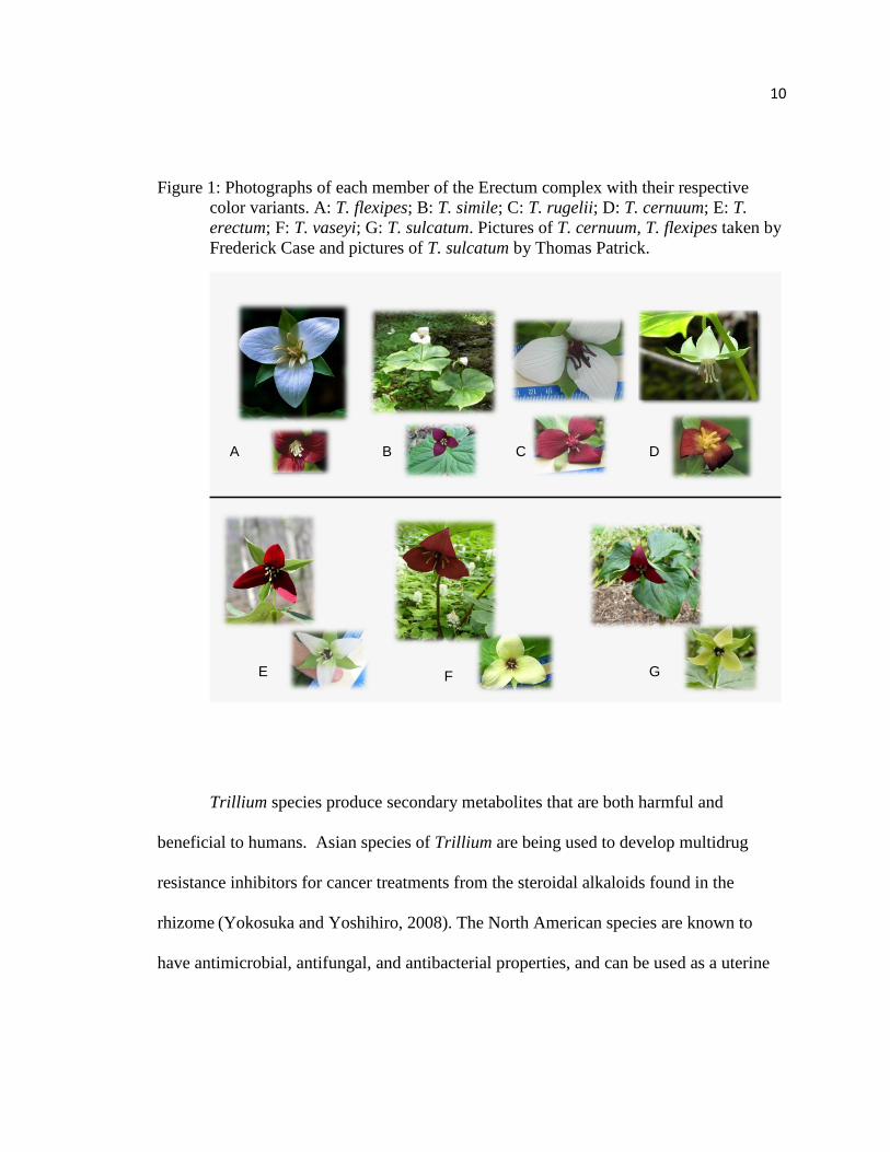
Figure 1: Photographs of each member of the Erectum complex with their respective

color variants. A: T. flexipes; B: T. simile; C: T. rugelii; D: T. cernuum; E: T.

erectum; F: T. vaseyi; G: T. sulcatum. Pictures of T. cernuum, T. flexipes taken by

Frederick Case and pictures of T. sulcatum by Thomas Patrick.

A B C D

E F G

Trillium species produce secondary metabolites that are both harmful and

beneficial to humans. Asian species of Trillium are being used to develop multidrug

resistance inhibitors for cancer treatments from the steroidal alkaloids found in the

rhizome (Yokosuka and Yoshihiro, 2008). The North American species are known to

have antimicrobial, antifungal, and antibacterial properties, and can be used as a uterine

11

stimulant (Case, 2008). Some parts of the plant can cause serious pain, injury, and even

death if consumed (Case, 2008).

Taxonomy

There is much debate surrounding the familial placement of Trillium and

arrangement of lower taxa within the genus. Trillium is currently treated as a member of

the family Trilliaceae by A. Weakley (Weakley, 2006), a family which first became

recognized in 1846 (Lindley cited in Farmer, 2006). Yet the Angiosperm Phylogeny

Group considers Trilliaceae to be synonymous with Melanthiaceae, and does not

recognize it as a separate entity (Stevens, 2001). Within the genus Trillium the pedicellate

flowered taxa (subgenus Trillium) and the sessile flowered species (subgenus

Phyllantherum) (Case and Case, 1997) have been separated. Subgenus Phyllantherum is

accepted as a monophyletic sub-group of 22 species, and an arrangement of lower taxa

within that group has been published and widely accepted (Farmer, 2006). Several

methods of cladistic analysis using a variety of data sets have led to resolution of several

different clades within the subgenus Trillium (Figure2: Farmer, 2006; Osaloo et al., 1999;

Ihara and Ihara, 1978). The most recent phylogenetic study by Farmer (2006) is

consistent with that of Osaloo et al. (1999, Figure 2) and shows that members of the

Erectum complex are monophyletic. Within the Erectum Complex relationships are

uncertain.

12

A

B

Figure 2. Phylogenetic relationships within the pedicellate Trilliums. A: Farmer

2006. B: Osaloo et al. 1999

A classification of lower taxa within subgenus Trillium based on morphological

characteristics such as ovary shape and color, stigma length and curvature, and stamen

13

morphology was defined by Barksdale (1939, Figure 3); which similarly to Farmer’s and

Millam’s molecular phylogenetic studies, differentiates T. undulatum Willdenow, which

has a 3-angled ovary, from the Grandiflorum group (T. grandiflorum (Michx.) Salisbury,

T. catesbei Elliot, and T. pusillum Michaux), which has a 6-angled ovary, and the

Erectum group (T. cernuum L., T. flexipes Rafinesque, T. simile Gleason, T. rugelii

Rendle, T. erectum L., T. sulcatum T. Patrick, and T. vaseyi Harbison), which has a 6-

angled ovary and rhombic leaves. The evolutionary relationships among taxa belonging

to the Erectum group remain unresolved (Millam, 2006; Farmer, 2006), with the current

taxonomic divisions between taxa within the complex based morphological differences

only.

Figure 3. Hypothesis of relationships in pedicellate Trillium based on ovary morphology

(Barksdale, 1939).

14

The Erectum Complex has been accepted as a monophyletic group within

subgenus Trillium (Farmer, 2006, Ihara and Ihara, 1978, Millam, 2006; Osaloo et al.,

1999). The complex is composed of the following taxa: Trillium cernuum, T. flexipes, T.

simile, and T. rugelii, which are typically white flowered; and T. erectum, T. sulcatum,

and T. vaseyi which are typically red flowered (Table 1 contains detailed morphological

descriptions, Appendix A). The goals of this project were to estimate the phylogenetic

relationships among members of the Erectum group, determine if significant levels of

introgression are present among taxa, and determine possible ecological factors affecting

introgression.

Syngameons & Hybrid Complexes

The prevailing theme behind the Biological Species Concept (BSC; Mayr, 1982)

is that species are groups defined by only the populations which are included in a

particular gene pool and excludes all others that are intrinsically reproductively isolated

from that gene pool (Coyne and Orr, 2004). This species concept defines discrete groups

of taxa in the strictest and sometimes the most inclusive sense. This definition has not

been satisfactory to some because it may mask the total variation and diversity present.

There are many of other species concepts that have been published and widely used in

taxonomy that are based on character state, evolutionary cohesion, and interbreeding

(Coyne and Orr, 2004). Either way you define a species there are problematic

exceptions, such as hybridization and introgression, that blur morphological

distinctiveness.

15

Many groups of taxonomically distinguished sister taxa are known to hybridize

naturally and produce fertile offspring (Coyne and Orr, 2004). Groups of naturally

hybridizing taxa can be referred to as syngameons (Lotsy cited in Stebbins, 1958), a

notable example being the White Oak syngameon found in California (Arnold et al.,

2004). These complexes are also referred to as semispecies (Grant, 1981), a term which

may be more descriptive of the true nature of their relationship with one another. Grant

describes semispecies as occurring during “various intermediate stages of divergence and

reproductive isolation, when populations are neither good races nor good species but are

connected by a reduced amount of interbreeding and gene flow.” (pg. 71 Grant, 1981).

Strictly speaking, groups of interfertile populations could be considered conspecific, but

Grant (1981) distinguishes these systems by limited gene exchange: “syngameons behave

like a well-isolated biological species on their outer boundary, but differ in their more

complex internal structure”. They are defined as “the most inclusive interbreeding

population system in a hybridizing species group” (pg. 74 Grant, 1981). Another type of

relationship can exist between hybridizing taxa: the hybrid complex. A hybrid complex is

distinct from a syngameon in that hybrid races or species within the group exhibit stable

reproduction, and there are high levels of introgression among populations which have

distorted the morphological boundaries between parent species (Grant, 1981). Although

the famed Louisiana Irises are thought to fit the syngameon model (Arnold et al., 2004),

they are probably a more accurate representation of a hybrid complex.

Members of the Erectum complex may be in the midst of a similar state of limbo

in their evolution and not much is known about the amount of genetic exchange that

occurs among taxa within the complex. The taxonomic limits are described and defined

16

by morphological characteristics, most of which are variable and overlap among species

(Table 1, Appendix A).

“Taxonomy is required to identify and monitor components of plant diversity to

ensure conservation and sustainable use” (United Nations’ Convention on Biodiversity

Article 7, page 20 Leadlay and Jury, 2006). Groups of taxa that are not fully diverged

and maintain levels of introgression are hard to differentiate taxonomically for practical

use in conservation management. When forming taxonomic groups it is important to

realize that assumptions about genetic cohesion and divergence within and among taxa

will be made by those creating management plans (Leadlay and Jury, 2006). Taxonomic

groups, unless otherwise specified in the literature, may be treated as independent gene

pools and managed without regard to historical gene flow between other taxa.

Understanding the reproductive relationships between groups of taxa can contribute to

information not only on current gene flow and phylogenic relationships but also the

future trajectory of the organism and the ecological factors that influence it. Character

state delineations do not always offer the same insights (Leadlay and Jury, 2006).

Barriers to Gene Flow

To address questions of species distinctiveness within hybrid complexes and

syngameons, it is necessary to know about paths of gene flow within the complex, be

able to quantify gene flow, and know something about the barriers to gene flow. Patterns

in the fertility relationships of plant species based are on life form and breeding system

(Grant, 1981). Grant describes one pattern, the “Geum” pattern, as a type of fertility

relationship often seen in “perennial herbs without prominent species-to-species

17

differences in floral mechanism” (Grant, 1981). This pattern is described as closely

related species which are interfertile, yet have compatibility barriers within the complex.

These taxa are predominantly outcrossed. Also, members of this complex would have

little difference in floral mechanism between species, and barriers that do exist among

species are due to extrinsic or ecological factors (Grant, 1981). This pattern describes the

apparent breeding system in the Erectum complex.

Since the taxa in the Erectum complex of Trillium are known to hybridize

successfully (producing fertile offspring) in wild populations, it is difficult to determine

the mechanisms that reinforce distinct gene pools in sympatric populations. Introgression

among taxa could make finding species-specific genetic markers difficult. A particular

allele may be fix in a population or taxa but if there is hybridization and back crossing

that allele may be shared with individuals outside of the population or taxa and therefore

could not be listed as a species or population marker. Measures of genetic distance may

correlate more with presence or absence of isolation barriers than with evolutionary

relationships. Based on Grant’s (1981) model of the typical fertility relationships among

perennials like Trillium, reproductive isolation barriers could be extrinsic (i.e.

ecological). These barriers could hold clues to the driving forces behind divergence in

this group. Since hybrids formed in this group are said to be developmentally normal and

fertile (Case and Case, 1997), there is no evidence that points to intrinsic barriers to gene

flow.

Members of the Erectum complex tend to be found in sympatric populations of

taxa from the opposite flower color group. The ranges described for most taxa do not

18

overlap (or scarcely so) with the ranges of similar flower colored taxa (Figure 4).

Trillium individuals may have relatively close pollen donors, shown to be within 2.2 m in

two species of pedicellate Trillium (Irwin, 2001). Seed dispersal by ants is common in

this genus and has been shown to influence the genetic structure within populations of T.

grandiflorum (Kalisz et al., 1999). These patterns suggest taxa not found in sympatric or

parapatric populations would have very little gene flow.

Two types of extrinsic barriers to gene flow may exist in Trillium: pre-zygotic

extrinsic barriers such as habitat isolation and post-zygotic extrinsic barriers such as

ecological inviability of hybrids (Coyne and Orr, 2004). The contrasting flower color

scheme in the Erectum Complex also suggests the presence of assortative mating via

pollinator preference. This type of extrinsic pre-zygotic mating barrier would allow taxa

with different colored flowers to remain distinct in sympatry (Coyne and Orr, 2004).

Assortative mating by pollinators happens when one particular group of pollinators visits

the same floral type in succession (Kearns and Inouye, 1993; Grant, 1981; Coyne and Orr

and Orr, 2004). A related concept that might also occur in a model of assortative mating

is floral constancy; this is a characteristic of an individual pollinator in which it visits the

same floral type repeatedly and in succession (Kearns and Inouye, 1993; Grant, 1981;

Coyne and Orr, 2004).

Assortative mating has been documented in red and white campions (Silene

dioica L. Clairv. and S. latifolia Poir.) using dyed pollen (Coyne and Orr, 2004) and

between white and pink phlox (Phlox pilosa L. and P. glaberrima L.) (Grant, 1981).

Phlox pilosa and Phlox glaberrima are both usually pink, but there is a white variant of

19

P. pilosa. These species are pollinated by the same species of Lepidoptera (Grant, 1981).

The white form is usually rare in populations where P. pilosa is the only species present,

but in sympatric populations with both species the white form is dominant (Grant, 1981).

Levin and Kerster (1967, cited in Grant, 1981) studied pollen movement between the

species and determined that five times as much pollen was deposited from P. glaberrima

to stigmas of the pink form of P. pilosa as to the white form (Grant, 1981). This gave the

white form a selective advantage because it received less pollen from outside of its own

species (Grant, 1981). Similarly, in the study by Coyne and Orr (2004), dyed pollen was

used to show pollinator isolation between red and white campions (Silene dioica and S.

latifolia), which overlap in some pollinators. The strength of the reproductive barrier

between the red and white species was found to be ca. 0.45, where 0 is no pollinator

isolation and one is complete assortative isolation (Coyne and Orr, 2004).

20

A) T. erectum distribution B) T. vaseyi distribution C) T. sulcatum distribution

D) T. flexipes distribution E) T. rugelii distribution F) T. simile distribution

Figure 4. Geographic distributions of Trillium Erectum complex taxa.

Rationale for Study

There is no immediate concern for the conservation of most Trillium species since

they are fairly abundant within their range. Yet because of their small ranges some

species are listed as “rare,” “threatened,” or “vulnerable.” Trillium simile is listed as

“rare” in both NC and SC, a “species of concern” in GA, and global status G3: vulnerable

(Weakley, 2010; NatureServe, 2010). Trillium sulcatum is a “species of concern” in GA

and the global status is G4 (Weakley, 2010; NatureServe, 2010). Trillium rugelii is on

the NC Watch List and listed as “rare” in SC (Weakley, 2010; NatureServe, 2010).

It is important to consider how likely it is that even the healthiest populations of

all species will be maintained in light of present day circumstances, such as Tsuga

21

canadensis die off and climate change. These circumstances have the potential to cause

dramatic shifts in the ecological forces that effect Trillium species in eastern forests

(Eschtruth et al., 2006; Crookston, 2010). Since Trillium species are extremely difficult

to cultivate from seed, many are poached from the wild. Deer herbivory is one of the

most prominent threats to Trillium populations, and management of deer herds could

mitigate any further harm (Vellend et al., 2003; Case and Case, 1997). Some species

have an exceptionally small range that covers areas susceptible to human development

(i.e. habitat loss), and some species have small, fragmented populations that may be

sensitive to loss of genetic diversity from the loss of populations and/or suitable habitat.

It is also important to consider that Trillium species are managed by state and

federal organizations according to current taxonomic delineations. There is the possibility

that these delineations are too narrow and do not include all interbreeding populations. In

other words they would not include all the individuals (or all of the genetic diversity)

necessary to sustain a minimum viable population, and management decisions based on

this could be detrimental to species diversity and population health. Evaluate these

species now, while they are still in sustained populations; and we can determine what

ecological and geographical features vital to maintaining diversity, seems wise. If these

species do become endangered, biologists the current body of knowledge, regarding

Trillium life history characteristics and gene flow among and within taxa, is inadequate

for creating proper management plans. It is recommended that information about genetic

diversity within and among taxa be used to guide conservation science (Leadlay and Jury

(2006).

22

Key barriers that influence genetic diversity within and among taxa in healthy

populations need to be examined. Once evaluated, this knowledge would also not only

provide valuable information to the scientific community for the subgenus Trillium, but

also contribute to the overall body of knowledge regarding biogeography in the Southern

Appalachians and to speciation mechanisms in general.

Study Site

The Southern Appalachian Mountains contain the highest diversity of Trillium

taxa in North America, making this an ideal place to study the relationships and gene

flow among sympatric populations. Field sites were chosen based on their isolation from

anthropogenic disturbance, population size (25-100 individuals), and abundance of

Trillium taxa present. Sites included Standing Indian Wildlife Management Area (Macon

County, NC N34.99972, W-83.46778), Balsam Mountain Preserve (Jackson County, NC

N35.39, W83.2), Wolf Creek Watershed area (Jackson County, NC), Great Smoky

Mountains National Park (Swain County NC, N35°33’01.98”, W83°29’33.08” and Sevier

County, TN N35.66833, W-83.4725), Frozenhead State Park (Anderson County, TN

N36.256, W-84.4690), Chattahoochee National Forest Chattooga district Black Rock

Mountain State Park (Rabun County, GA; N34.908146, W -83.409536), Sumter National

Forest Whetstone district, Whitewater Falls area (Oconee County, SC N34.8619 W-

83.1919), Western Carolina University picnic area (Jackson County, NC; N35.315632,

W-83.188382), Nantahala Gorge along Hwy 64 (Swain/Madison Counties, NC; N

35.335304, W -83.622677). Since these taxa are known to hybridize in native populations

23

with parapatric sister taxa, individuals from the interior and the perimeter of populations

were collected.

24

CHAPTER TWO: POLLINATOR ISOLATION

Objective

The objective to this portion of the study is to identify extrinsic interspecific

mating barriers pertaining to pollinator fidelity.

Hypothesis

I hypothesize that assortative mating or floral constancy based on flower color is

exhibited by pollinators, and provides a potential barrier to gene flow between red

flowered and white flowered taxa. This will be tested by tracking the distribution of

marked pollen and by pollinator observations. If this is true then I would expect to see an

insignificant amount of pollen transferred between red and white flowers.

Materials and Methods

Pollinator observations were attempted by performing observations of patterns of

floral constancy among taxa and individuals. Visual observations of pollinator behavior

were made to see if pollinators would consistently visit flowers of a similar type. Two

10m x 10m plots in Balsam Mountain Preserve, Jackson County, NC, were used to test

for floral constancy by tracking dyed pollen. One plot was done in April 2009 and the

second in May 2009. Histochemical dyes were injected into the anther flaps prior to

dehiscence; the pollen grains absorb the dyes (which are visible to the naked eye) (Kearns

et al., 1993). Twenty-eight individuals of each white taxa and each red taxa in both plot

had their anthers stained. The first plot contained T.grandiflorum (stained orange) and

25

T.erectum (stained blue); the second plot contained T.erectum (stained blue), T.vaseyi

(stained green), and T.rugelii (stained magenta). The second plot contained two red

species and only one white species but frequency of red and white individuals was

similar. After two weeks of pollinator activity (to allow for pollen tube growth) the

stigmas were collected and analyzed. We were only able to collect data from half of the

individuals in one plot. One plot was highly disturbed and most individuals trampled by

hikers; the other plot was in a more remote drainage but there was a high amount of

insect herbivory on the anthers and stigmas. Quantitative data were scored for the

different colors of pollen seen on each stigma and the approximate percentages of each

present. A chi-squared contingency table was used to test the significance of cross

pollination among taxa and among different colored taxa. .

Results

Eight out of 45 stigmas collected contained pollen from an individual with a

different petal color (18%, Table 2, Appendix B). The resulting test statistic was X² =

16.2 (df=1, p=0.05, x=3.84); therefore we reject the null hypothesis that pollination was

random between red and white flowered individuals. Eight of 30 stigmas (27%) collected

contained pollen from an individual with the same color flower but from a different

taxon. The resulting test statistic was X² = 3.27, df=1, P=0.07; therefore we fail to reject

the hypothesis that pollination was random between different taxa of the same flower

color. During the course of this study approximately 12 hours of observations were done

to try to confirm the types of pollinators that were described by Barksdale (1939).

Lepidoptera, Hymenoptera (ants, carpenter bees, bumble bees, sweat bees, and carpenter

ants), and several species belonging to the order Araneae were all observed in or on

26

Trillium reproductive organs (although the spiders were never observed moving from one

plant to another). Another interesting observation is that while it has been reported that

some insects eat the elaiosome from the seeds (Kalisz, 1999), there was not a large

amount of insect herbivory on the ovary itself. By mid to late June, all or at least some

part of the petals, stigmas, styles and stamen had been eaten from almost every

individual, yet most of the ovaries were untouched.

Discussion

The lack of significant pollen dispersal to plants of different floral color supports

assortative mating between different color forms of these taxa. The data also supports a

higher significance of pollination by flowers within the same color petals opposed to

random pollination. This supports the hypothesis that similar colored taxa are genetically

isolated by an incomplete and unstable extrinsic barrier, assortative mating via pollinator.

Also, when you consider that these taxa are considered to be separate species it is

interesting to note that the degree of cross pollination among all taxa, at least as judged

by the presence of non-self pollen on the stigma, is significant (X²= 7.2, df=1, P=0.007).

The presence of pollen from other taxa does not confirm cross fertilization. The

germination of neither conspecific nor heterospecifc pollen was able to be observed so

there is no data on the successful fertilization of plants pollinated by conspecific pollen

verse plants pollinated by other taxa. Since hybrids are known to form in the wild, it is

known that cross fertilization occurs. But since it is not known if all pollen, conspecific

and from other taxa, is equally as likely to germinate it cannot be assumed that assortative

mating via pollinators is the only mechanism acting as a barrier to gene flow.

27

CHAPTER THREE: GEOGRAPHIC AND ECOLOGICAL ISOLATION

Objectives

The objectives of this portion of the study are to take an exploratory look at

identifying extrinsic interspecific mating barriers pertaining to geographic isolation and

dissimilar habitat characteristics and quantifying the relationship between potential

geographic and ecological mating barriers with the presence of certain taxa.

Hypothesis

I hypothesized that taxa of the same flower color in the Erectum complex are

found in different habitat types, occupy separate ecological niches, or have substantial

geographical barriers between them that minimize introgression between taxa. If this is

true then I would expect to observe substantial differences in the habitats of taxa with the

same floral type. These differences in habitat preference might include mutually

exclusive conditions pertaining to geologic formation, watershed, average precipitation,

average temperature, soil type, or forest type.

Materials and Methods

Initial observations were made by entering known locations of all six taxa from

herbarium data and field site collection data into a GIS shape file format imported over a

US thematic base map, and then overlaying layers of USGS data on temperature,

hydrology, topography, and geologic formation/soil type data. Values for each USGS

category at each plant location were extracted using Spatial Analyst (ArcGIS ver. 9.3.1,

28

2009. Redlands, CA: Environmental Systems Research Institute) and appended into a

table. The data were analyzed in R (R: A language and environment for statistical

computing. R Foundation for Statistical Computing, Vienna, Austria. ISBN 3-900051-07-

0) by creating a Multicategory Logit Regression model (Agresti, 2007) and calculating

an Analysis of Deviations table (ANOVA function in R), then forming effect plots that

show the probability of a member of each taxon being located in each habitat condition.

Results

Values extracted from USGS data layers for geologic formation, watersheds,

average precipitation, average yearly temperature, soil type, and forest type are listed in

Table 3 (Appendix C). The Tennessee River outlined the border between the ranges of

same colored species (Figure 5).

Figure 5: County-level distribution maps depicting an example of geographic

isolation between taxa. The map to the left depicts geographic isolation between two red

flowered species; the red blocks represents the distribution of T. sulcatum and the orange

blocks represents the range of T. vaseyi. The map on the right depicts geographic

isolation between two white flowered species; the green blocks represents the range of T.

flexipes, and the blue blocks represents the range of T. rugelii. The center map shows the

Tennessee River in blue.

29

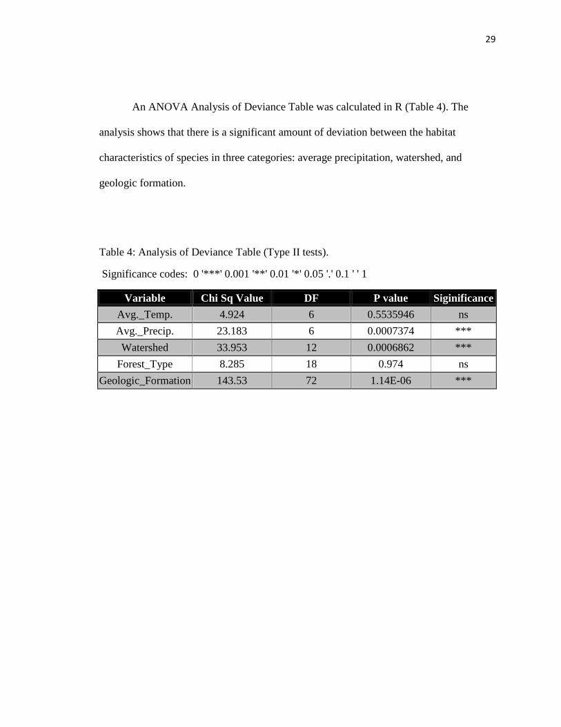
An ANOVA Analysis of Deviance Table was calculated in R (Table 4). The

analysis shows that there is a significant amount of deviation between the habitat

characteristics of species in three categories: average precipitation, watershed, and

geologic formation.

Table 4: Analysis of Deviance Table (Type II tests).

Significance codes: 0 '***' 0.001 '**' 0.01 '*' 0.05 '.' 0.1 ' ' 1

Variable Chi Sq Value DF P value Siginificance

Avg._Temp. 4.924 6 0.5535946 ns

Avg._Precip. 23.183 6 0.0007374 ***

Watershed 33.953 12 0.0006862 ***

Forest_Type 8.285 18 0.974 ns

Geologic_Formation 143.53 72 1.14E-06 ***

30

Avg._Temp. effect plot

Avg._Temp.

Sp

eci

es

(pro

ba

bili

ty)

0.20.40.60.8

46 48 50 52 54

: Species erectum

0.20.40.60.8

: Species erectum_album

0.20.40.60.8

: Species flexipes

0.20.40.60.8

: Species hybrid

0.20.40.60.8

: Species rugelii

0.20.40.60.8

: Species simile

0.20.40.60.8

: Species vaseyi

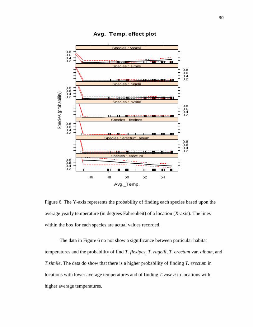
Figure 6. The Y-axis represents the probability of finding each species based upon the

average yearly temperature (in degrees Fahrenheit) of a location (X-axis). The lines

within the box for each species are actual values recorded.

The data in Figure 6 no not show a significance between particular habitat

temperatures and the probability of find T. flexipes, T. rugelii, T. erectum var. album, and

T.simile. The data do show that there is a higher probability of finding T. erectum in

locations with lower average temperatures and of finding T.vaseyi in locations with

higher average temperatures.

31

Geologic_Formation effect plot

Geologic_Formation

Sp

ecie

s (

pro

ba

bility)

0.2

0.6

CZbg CZmv CZtp CZve DSs Kc Mc PPg PzZg PzZu TRd Zb Zsr

: Species erectum

0.2

0.6

: Species erectum_album

0.2

0.6

: Species flexipes

0.2

0.6

: Species hybrid

0.2

0.6

: Species rugelii

0.2

0.6

: Species simile

0.2

0.6

: Species vaseyi

Figure 7. The Y-axis represents the probability of find each species based upon the geology type

of a location (X-axis).

The data in Figure 7 show a low degree of probability of finding T. flexipes, T.

rugelii, T. erectum var. album, and T.simile in one particular geologic formation over

another. The data also shows a high probability of finding T.vaseyi and T. erectum over

particular and opposing geological formations from one another.

32

Watershed effect plot

Watershed

Sp

ecie

s (

pro

ba

bility)

0.20.40.60.8

Neuse New Savannah

: Species erectum

0.20.40.60.8

: Species erectum_album

0.20.40.60.8

: Species flexipes

0.20.40.60.8

: Species hybrid

0.20.40.60.8

: Species rugelii

0.20.40.60.8

: Species simile

0.20.40.60.8

: Species vaseyi

Figure 8. The Y-axis represents the probability of finding each species based upon the watershed,

the X-axis, in which it was located (“New” stands for “New River” watershed).

The data in Figure 8 show a higher probability of T. vaseyi being in the Neuse

watershed, of T. erectum of being in the New River or Savannah watersheds, and of T.

simile and T. rugelii of being in the Savannah watershed over the others.

33

Avg._Precip. effect plot

Avg._Precip.

Sp

ecie

s (

pro

ba

bility)

0.20.40.60.8

50 60 70 80 90

: Species erectum

0.20.40.60.8

: Species erectum_album

0.20.40.60.8

: Species flexipes

0.20.40.60.8

: Species hybrid

0.20.40.60.8

: Species rugelii

0.20.40.60.8

: Species simile

0.20.40.60.8

: Species vaseyi

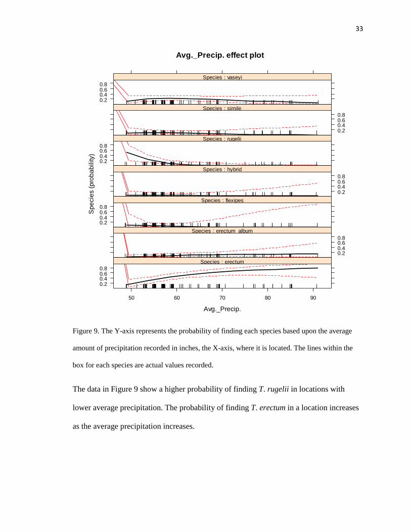
Figure 9. The Y-axis represents the probability of finding each species based upon the average

amount of precipitation recorded in inches, the X-axis, where it is located. The lines within the

box for each species are actual values recorded.

The data in Figure 9 show a higher probability of finding T. rugelii in locations with

lower average precipitation. The probability of finding T. erectum in a location increases

as the average precipitation increases.

34

Forest_Type effect plot

Forest_Type

Sp

ecie

s (

pro

ba

bility)

0.2

0.6

Maple/Beech/Birch Maple/Beech/Birch_ Oak/Hickory_GroupWhite/Red/Jack_Pine_

: Species erectum

0.2

0.6

: Species erectum_album

0.2

0.6

: Species flexipes

0.2

0.6

: Species hybrid

0.2

0.6

: Species rugelii

0.2

0.6

: Species simile

0.2

0.6

: Species vaseyi

Figure 10. The Y-axis represents the probability of find each species based upon the USFS Forest

Type, on the X-axis, of the location in which it is located. There are two subsections of the Sugar

Maple/Beech/Yellow Birch forest type which were not distinguished in the metadata for the layer

in ArcGIS.

Figure 10 shows that T. vaseyi is most likely to be found in a Sugar

Maple/Beech/Yellow Birch forest then other forest types. Trillium rugelii is slightly more

likely to be found in a Sugar Maple/Beech/Yellow Birch forest then other forest types.

35

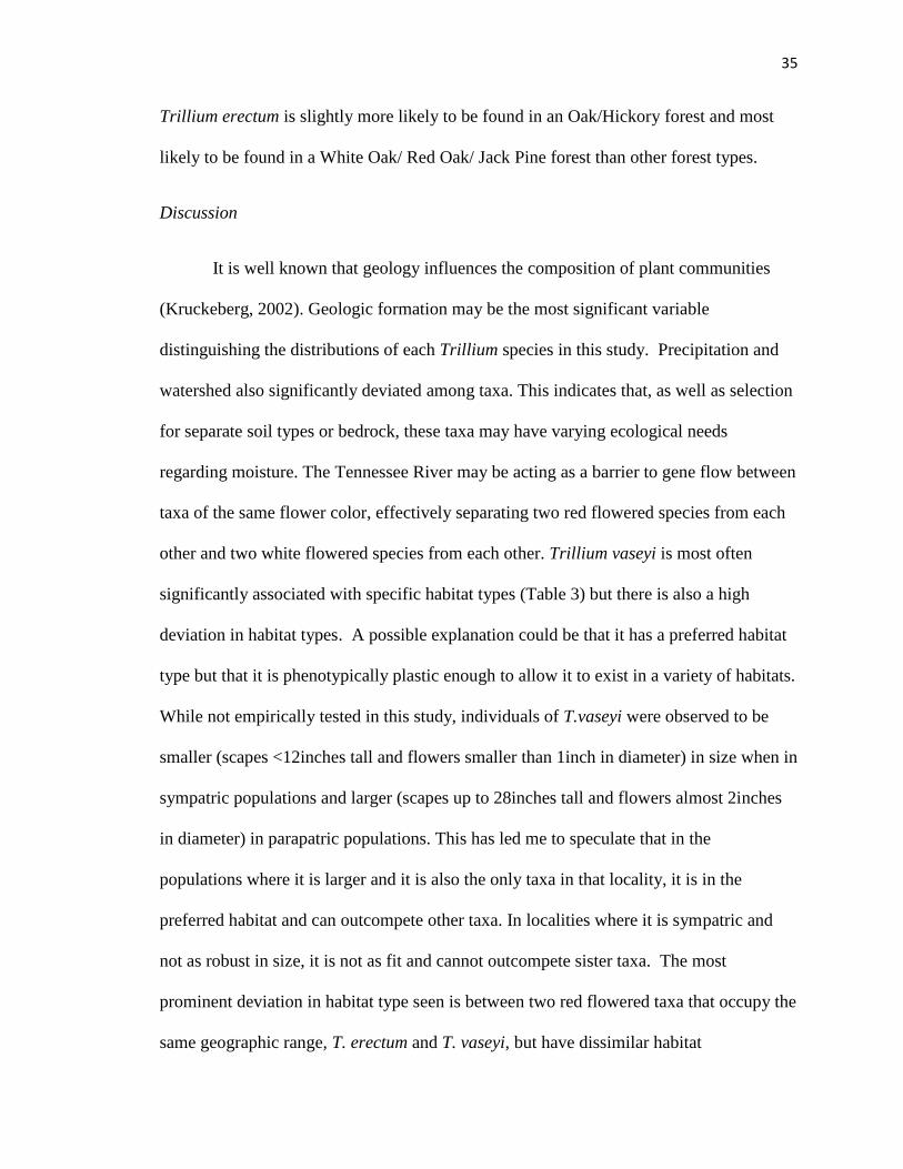
Trillium erectum is slightly more likely to be found in an Oak/Hickory forest and most

likely to be found in a White Oak/ Red Oak/ Jack Pine forest than other forest types.

Discussion

It is well known that geology influences the composition of plant communities

(Kruckeberg, 2002). Geologic formation may be the most significant variable

distinguishing the distributions of each Trillium species in this study. Precipitation and

watershed also significantly deviated among taxa. This indicates that, as well as selection

for separate soil types or bedrock, these taxa may have varying ecological needs

regarding moisture. The Tennessee River may be acting as a barrier to gene flow between

taxa of the same flower color, effectively separating two red flowered species from each

other and two white flowered species from each other. Trillium vaseyi is most often

significantly associated with specific habitat types (Table 3) but there is also a high

deviation in habitat types. A possible explanation could be that it has a preferred habitat

type but that it is phenotypically plastic enough to allow it to exist in a variety of habitats.

While not empirically tested in this study, individuals of T.vaseyi were observed to be

smaller (scapes <12inches tall and flowers smaller than 1inch in diameter) in size when in

sympatric populations and larger (scapes up to 28inches tall and flowers almost 2inches

in diameter) in parapatric populations. This has led me to speculate that in the

populations where it is larger and it is also the only taxa in that locality, it is in the

preferred habitat and can outcompete other taxa. In localities where it is sympatric and

not as robust in size, it is not as fit and cannot outcompete sister taxa. The most

prominent deviation in habitat type seen is between two red flowered taxa that occupy the

same geographic range, T. erectum and T. vaseyi, but have dissimilar habitat

36

characteristics (Table 4). During field observations, there were never more than a dozen

individuals of T. erectum or T. vaseyi in sympatric populations with one another (Table 7,

Appendix D). From the literature available there are certain species that are known from

field observations to be consistently found in certain habitat types (Case and Case, 1997).

These have yet to be empirically tested to determine whether or not similar colored taxa

select for dissimilar habitat conditions. In this preliminary work, it appears that at least

two taxa similar colored taxa are selecting for dissimilar habitat conditions. This supports

the hypothesis that similar colored taxa gain at least partial reproductive isolation through

ecological isolation. In future studies direct examination of habitat characteristics like

acidity, elevation, and moisture would be ideal to use in attempting to find differences

among taxa habitat selection.

37

CHAPTER FOUR: CHOLOROPLAST DNA SEQUENCING

Objective

The objectives in this portion of the study are to construct a phenogram and

genetic network based on genetic distances from cpDNA sequence data to depict possible

phylogenetic relationships among the members of the Erectum complex.

Figure 11. Hypothesized Evolutionary Relationships: The black arrows indicate direct

ancestor-descendant relationships and red arrows indicate introgression contributing to

the speciation event. Red text indicates red-flowered taxa; blue text indicates white-

flowered taxa (This proposed model is not intended to represent current gene flow, but to

describe historic paths of of gene flow over the development of the complex)

I hypothesize that the common ancestor of the Erectum complex may have been

similar to the extant T. erectum species. Trillium erectum is known to have the widest

variation in morphological characteristics in the Erectum group. In taxa such as these,

38

individuals with divergent phenotypic variations could have become isolated by

pollinator preference for specific floral types (Coyne and Orr, 2004). In this model

(Figure 11) there would have been two color forms (red and white) of the ancestral taxon,

which became isolated by pollinator preference. Within each clade further divisions

would have occurred based on habitat preference (black arrows). Morphological

differentiation from the ancestor would have been promoted through introgression from

other semi-species (red arrows, Figure 11). The red-flowered form of the ancestral T.

erectum ultimately gave rise to T. sulcatum, T. erectum, and T. vaseyi; and the white-

flowered form gave rise to T. erectum var. album, T. simile, T. flexipes, T. rugelii, and

T.cernuum.

If this model (Figure 11) holds true I would expect to see the most variation,

greatest number of haplotypes and greatest number of polymorphic loci to be found in T.

erectum. I expect to see higher genetic identity between white-flowered taxa then

between white-flowered and red-flowered taxa. If these groups within the Erectum

complex are distinct taxa, then I would expect to see an average genetic distance within

the genera of 0.07, among species within the complex of 0.04 from cpDNA sequence

data (based on averages from a combined matK and ITS data set; Farmer, 2006), and

0.97-4.17% variation within the genus (Shaw et al., 2005).

39

Materials and Methods

A total of 203 fresh tissue collections (Table 29, Appendix D) and 12 voucher

specimens of five taxa and one variety of Trillium were collected from 11 sites: six in

NC, three in TN, and two in GA. Voucher specimens are deposited in the herbarium at

Western Carolina University (WCUH). For taxa for which fresh leaf tissue could not be

obtained, DNA extractions were attempted from herbarium material.

Leaf tissue from individuals of each taxon belonging to the Erectum group was

sampled at each field site in which they were present. One leaf was taken from between

one and twenty-four individuals from each taxon. Prospective hybrids (individuals with

intermediate phenotypes) were also sampled when present. Samples were collected on

dry ice, flash frozen in liquid nitrogen, and stored at -70ºC until DNA extractions could

be made.

Total DNA was obtained from leaf tissue frozen in liquid nitrogen using a

modified CTAB extraction (Doyle and Doyle, 1987) and herbarium specimens using

either a DNeasy Plant Mini kit (Qiagen Corporation, Valencia, California). Primers for

the rpl32-trnL intergenic spacer region (Shaw et. al 2007) were used to amplify non-

coding cpDNA using standard polymerase chain reaction (PCR). The PCR cycle

consisted of the following steps: template DNA denaturation at 80°C for 5 min, 30 cycles

of denaturation at 95°C for 1 min, primer annealing at 50°C for 1 min, a ramp of 0.3°C/s

to 65°C, and primer extension at 65°C for 4 min; followed by a final extension step of 5

min at 65°C (Shaw et. al 2007). Successful amplification was confirmed by running

samples in a 1% agarose gel stained with ethidium bromide and quantity was measured

40

using a micro-volume spectrophotometer (Nanodrop). The samples were purified prior to

sequencing using QIAquick PCR Purification Kits (Qiagen Corporation, Valencia, CA).

The samples were then loaded with the sequencing primers on to 96-well plates and

shipped to the Genomic Sciences Laboratory (NC State University, Raleigh, NC) for

sequencing and capillary electrophoresis on a 3700 Genetic Analyzer (Applied

Biosystems). Subsequent electropherograms were edited and aligned in Sequencher

software (GeneCodes Corp., Ann Arbor, MI). Sequencher was used to view

chromatograms, edit ambiguous base calls, and trim, and align the sequences. PAUP*,

vers. 3.1.1 (Swofford, 1993) and TCS, vers. 1.21 (Clement et al., 2000) were used to

calculate neighbor-joining phenograms, compute genetic distances, and create a genetic

network calculated using the uncorrected-p method. Sequences of Trillium grandiflorum

and Trillium camschatense (downloaded from GenBank) were used as representative

outgroups in the analyses.

Results

A total of 108 individuals were successfully sequenced in both directions with the

trnL-rpl32 primers. The total number of bases sequenced was 826, including 49 variable

characters in the ingroup and 39 parsimony informative characters. Sequences from

forward and reverse primers did not overlap, so each end of the spacer region was

analyzed separately. From the forward end (rpL32 end) 445 bases were sequenced (7

variable and 4 informative), and this included a portion of the rpL32 coding region. From

the reverse end (trnL end) 381 bases were sequenced (42 variable and 39 informative)

and all were within the intergenic spacer region.

41

No species-specific haplotypes were observed. A genetic network was created in

TCS linking haplotypes that contain members of several taxa (Figure 12). The individuals

belonging to each haplotype are listed in Table 5. The average genetic distance between

T. camschatcense and members of the Erectum complex is 0.07. The genetic distance

among taxa within the complex is 0.003. The genetic distance between members of the

same taxon is 0.0007. Results from an ANOVA comparing variation within a taxon to

variation between ingroup taxa were not significant (df=1; F=0.0919, p=0.721). Results

from an ANOVA comparing variation within the complex with variation between the

members of the complex and the outgroup were highly significant (df = -1; F= 170.45,

p= 2.2eˉ16). The average Nei’s pairwise genetic identity between red and white taxa is

99.74, between red taxa is 99.62, and between white taxa is 99.81. Trillium vaseyi was

found to contain the most genetic variation within a taxon. The TCS parsimony network

created (Figure 12) shows that there are only two haplotypes that are specific to one

taxon. The majority of the individuals in the network clump in to one haplotype and the

two largest haplotypes contain individuals collected from multiple taxa and localities. A

Neighbor Joining phenogram was created in PAUP (Figure 13). The diagram does not

show complete segregation of individuals by taxon or by locality but for the most part

individuals identified as T. vaseyi, T. rugelii and T.erectum do group with their own taxa.

42

Figure 12: Genetic parsimony network created using TCS. Numbers represent the number

of individuals belonging to each taxon that were placed in that haplotype. Haplotypes that

were not connected to the network are not shown.

43

Figure 13: Neighbor Joining Phenogram created in PAUP. The location of each taxon is

inserted after the name at the end of each branch. The branch lengths are proportional to

genetic distance values.

44

Discussion

The genetic identity values show that the distance between T. camschatcense and

its American sister taxa meet expectations based on the assumption that they are separate

species in the same genus, but the distance values within the complex are an entire order

lower than would be expected even for members of the same species. Previous research

by Farmer (2006) using ITS and matK combined sequence data show the average genetic

distance among members of the same genus in the family Trilliaceae was 0.07 and within

species was 0.04 (Farmer, 2006). The average genetic identity between individuals was

99.86, considering the average identity between members of the complex was 99.93 there

appears to be more variation in that one “species” then between all “species”. The genetic

identity between white flowered taxa was higher than the distance between all members

of the complex, this suggest a stronger relationship amongst them as compared to the rest

of the complex. Nine haplotypes were created using TCS that included 52 individuals

(Table 5). A map was created using ArcGIS (Figure 15). While none of the haplotypes

were exclusive to only one taxon or locality when mapped, the groupings do show

segregation into a large cluster on the eastern side of the Appalachian Mountains and

individuals near the crest and the northwest side in another. The rest of the haplotypes

include a few individuals from the foothills at the southern tip of the mountain range. The

distribution of cpDNA haplotypes may be more representative of historical relationships

due to isolation in glacial refugia (Gonzales et al, 2008) than divergent phylogenetic

groupings.

45

Figure 14: Average Genetic Identity Values.

46

Figure 15: Geographic distribution of haplotypes created in TCS from cpDNA sequence

data. Each color represents a separate haplotype.

Table 5: Haplotypes created in TCS based on cpDNA sequences. E: T.erectum, A:

T.erectum var. album, R: T.rugelii, S: T.simile, V: T.vaseyi, F: T.flexipes

Haplotype Individuals included

Haplotype1 104A, 110A, 12R, 38E, 107A, 48ExR, 101E, 95E, 112E,118F, 200S, 22E, 29E, 74E, 47E, 73E, 76E, 91E, 37A, 95E, 201S, 29E, 94E, 38E, 28E, 104E

Haplotype2 62V, 50V, 4ExR, 2R, 64V, 164V, 163V, 152V, 10R, 12R, 58V, 147V, 49V, 12R, 149V, 148V, 65V

Haplotype3 301S

Haplotype4 118F, 131F

Haplotype5 70V

Haplotype6 2R

Haplotype7 25E, 118F

Haplotype8 132V

Haplotype9 131F

46

CHAPTER FIVE: ALLOZYME ELECTROPHORESIS

Objectives

The objectives of this portion of the study is to determine the relationships among

syngameons it may be helpful to look for the types of molecular variation typically found

within populations of the same species, such as allozyme variation between holotypes (an

organism exhibiting the typical character states described for a species) from isolated

populations of each species compared with known hybrids (Arnold et al., 2004). This has

been used successfully with a variety of other herbaceous plants; determining

relationships in Prosopis (Bessega et al., 2005; Saidman and Vilardi, 1987), the

phylogeny of Lathyrus (Brahim et al., 2002), genetic variation and hybridization in

Orchis laxiflora and Orchis palustris (Arduino et al., 1996), measuring genetic

distinctiveness and introgression in Carex (Tyler, 2003), and for showing patterns of

introgression and hybrid speciation in the Louisiana irises (Arnold et al., 1990).

My objectives were to find species-specific markers for as many Erectum species

as possible. These may be in the form of fixed alleles or fixed allelic frequencies for

particular allozyme loci. To determine the level of introgression, genetic distance,

inbreeding, and heterozygosity values for each taxa and locality were calculated.

Hypotheses

If these groups within the Erectum complex are distinct taxa, then I expect to see

values of genetic identity to be in the range of 0.956 within species, and genetic identity

48

values to be in the range of 0.67 (+/- 0.04) between for allozyme data (Soltis and Soltis,

1989; Gottlieb, 1981). I would also expect the genetic distance between different Trillium

species growing in allopatry to be greater than the genetic distances between different

species growing in sympatric populations (Solits and Soltis, 1989); If there is a

significant introgression currently occurring, then genetic identity values should be

higher among sympatric species than allopatric species.

Materials and Methods

A total of 203 fresh tissue collections (see Table 29, Appendix E for detailed list)

and 12 voucher specimens of five taxa of Trillium and one variety were collected from 11

sites; seven in NC, three in TN, two in GA. Voucher specimens are deposited in the herbarium

at Western Carolina University (WCUH).

Leaf tissue from individuals of each taxon belonging to the Erectum group was

sampled at each field site in which they were present. One leaf was taken from between

one and twenty-four individuals from each taxon. Prospective hybrids (individuals with

intermediate phenotypes) were also sampled when present. Samples were collected on

dry ice, flash frozen in liquid nitrogen, and stored at -70ºC until protein extractions could

be made.

Allozyme electrophoresis was used to detect the presence of allelic variations in

loci that are known to have variations in T. erectum (Irwin, 2001; Griffin and Barrett,

2004). Preliminary trials performed in Dr. Jim Hamrick’s lab at the University of Georgia

in Athens were used to determine which allozyme loci are polymorphic within this

species complex. Small portions of leaf tissue (1cm²) were ground in liquid nitrogen

49

using a mortar and pestle. The proteins were extracted using the buffer from Wendel and

Parks (1982). The extractions were absorbed on to Whatman no.3 wicks. After the trials

it was determined that horizontal starch gel-electrophoresis would be performed using

12% gels with three buffer systems: system 4 to resolve uridine diphosphoglucose

pyrophosphorylase (UGPP); system 34/40 (Cheliak and Pitel, 1984) used to resolve

menadione reductase(MNR), diaphorase (DIA), phosphoglucose isomerase (PGI),

peroxidase (APER); system -8 to resolve fluorescent esterase (FE). Recipes were

modified from Soltis et al. (1983) and Wendel and Weeden, Chapter 1, in Soltis and

Soltis (1989); the recipe for DIA and system 34/40 buffer from Cheliak and Pitel (1984).

Once the gels were been scored the allele frequencies were analyzed using GenAlEx

software (Peakall and Smouse, 2006) by locality, by taxon, by taxon and locality, by

color, and by color and locality. Nei’s genetic distances, allele frequencies, Hardy

Weinberg statistics, haplotypes, an AMOVA, heterozygote frequencies, and F-statistics

were calculated in each analyses.

Results

A total of 14 enzymes in three buffer systems were tested on 72 samples. Suitable

resolution was achieved in 12 enzymes for a total of 16 possible loci for analysis (Table

6, Appendix D). In the interest of time and money the seven best loci were selected for

the final run: diaphorase (DIA), aspartate aminotransferase (ATT), menadione (MNR1 &

MNR2), fluorescent esterase (FE), uridine diphosphoglucose pyrophosphorylase (UGPP),

glucose-6-phosphate isomerase (PGI). PGI was used despite getting no resolution in the

trials since it was believed to have been due to lab error; when PGI was run with the rest

of the samples there was still inadequate resolution to be reliably read.

50

For final analysis, data were collected for four loci from 199 samples (Table 7,

Appendix E). There were not enough data obtained from the other three loci to be used in

analysis, resolution of bands was not sufficient for accurate data collection. Genetic

distances and identities between taxa are recorded in Table 8 and Table 9 (Appendix D).

The average identity value is 0.878; the expected for species is 0.67±0.04 (Soltis and

Soltis, 1989). The average identity value by locality is 0.75 and the average distance is

0.32 (Table 10 and Table 11). Analysis of molecular variance indicated that the largest

amount of variation is found within taxa, 88% (Table 12, Appendix D). Trillium erectum

and the white variety T. erectum var. album shared similar allele frequencies at all loci,

yet T. erectum showed a slight deficiency in heterozygotes (Table 13, Appendix D). All

taxa significantly deviated from HWE in at least one locus (Table 21, Appendix D).

When individuals were grouped by locality the populations meet HWE expectations more

frequently than expected. When grouped by flower color data show a slight deficiency in

heterozygotes (Table 14, Appendix D). For white taxa the mean observed heterozygosity

(Hο) = 0.347 SE = 0.09 and the mean expected heterozygosity (He) = 0.484 SE = 0.019.

For red taxa mean Hο = 0.329 SE = 0.078 and the He = 0.483 SE = 0.062. We see higher

observed heterozygosity when individuals are lumped by locality rather than taxon. The

data show slightly higher genetic identity values than expected when considering them

separate taxa. When grouped by locality regardless of taxa, identity values are still fairly

high considering some of these populations are hundreds of miles apart or may not

contain the same taxa. When analyzing variation within groups of sympatric individuals

16% of the variation is found among localities, 31% among individuals within a locality,

51

and 54% within individuals (Figure 17 &Table 15, Appendix D). The Fst value among

taxa was 0.134 SE=0.016 and the Fst value among localities was 0.318 SE=0.067 (F-

statistics are reported in tables 20 and 23, Appendix D).

There were three populations of T. vaseyi that were parapatric with other taxa

(Whitewater Falls, Warwoman, and Black Rock Mtn) and one population that was

sympatric with two other taxa (Rainbow Falls ). When you compare the genetic distance

between populations of T. vaseyi which were parapatric with other taxa they had a higher

genetic identity among themselves than with populations of T. vaseyi that were sympatric

with other taxa (Table 16, Appendix D).

The white flowered form of T.erectum shows diverging allele frequencies at two

loci compared to the red variety in the population from Clingman’s Dome where they are

sympatric (Table 27). The allele frequencies of all populations, regardless of allopatry or

sympatry, of the white and red do not diverge significantly (Table 19).

Discussion

The data collected for populations of T.vaseyi support the hypothesis that the

allozyme data are showing introgression between taxa in sympatric populations. The data

was not conclusive for the complex as a whole; there was no distinct pattern between

sympatry and genetic distance among all taxa. This may have been due to sampling error

or lack of power from small sample sizes from certain populations or the patterns of gene

flow between individuals vary by taxon compounded by varying amounts of gene

exchange occurring in each locality. The Fst values show greater divergence among

populations then among taxa; which also supports the hypothesis that there is

52

introgression and suggests that current introgression could be influencing patterns of

identity. This is reiterated in the data from an AMOVA (Figure 18). It shows the largest

amount of variation is between individuals, indicating that a large portion of the variation

could be more or less random. The variation among taxa is still greater than the variation

among localities. When lumped by taxa rather than locality, you see a greater deviation

from HWE in the data set. This could suggest that evolutionary forces such as drift,

selection, and random mating act more on the local populations as a whole then on each

individual taxon.

The differences in allele frequencies of different colored taxa in GSMNP may be

due to assortative mating but the similar. In sympatric populations of the white and red

varieties of T.erectum, the differences in allele frequencies could have been caused by

selection (Conner and Hartl, 2004). These data may support previous data on assortative

mating. Since only two loci are affected then the cause would have to be some type of

selection, drift and gene flow would affect all loci equally (Conner and Hartl, 2004).

The higher than expected homozygosity found among all white flowered taxa suggest

non-random mating (Conner and Hartl, 2004) which also supports our hypothesis on

assortative mating.

53

Figure 16: Geographic distribution of haplotypes within localities from allozyme data.

Figure 17: Distribution of Molecular Variance from AMOVA created in GenAlEx.

Regions represent variance by locality, populations are comprised of taxa.

54

CHAPTER SIX: SYNTHESIS AND DISCUSSION

In the study of systematics within the Trillium Erectum complex the goal is to be

able to answer six key questions about the taxa: 1) what are the taxonomic groups, 3)

when did they evolve, 4) where did they evolve and where do they now exist, 5) why are

the current populations structured the way they are and 6) how did they become that

way? This discussion will attempt to address the questions of who or what are the

members of the Erectum complex, when might divergence have begun to occur, and

lastly what might have influenced their evolution historically and presently.

Who are the members of the complex and what should be treated as distinct

taxonomic units? Currently the taxonomic treatments based on morphology have proved

to be impractical for use in the field due to hybridization and development of local

ecotypes. I do not disagree that there are at least eight groups of historically divergent

taxa within this complex and within each of those groups there is the possibility of further

divisions into describable varieties of each taxon. The hierarchical level of classification

that each taxon should receive, however, is debatable.

Taxonomy is a decisive component in the quest to quantify biodiversity (Stussey

in Leadlay and Jury, 2006). The rank of classification will ultimately impact how the

genetic diversity is maintained/ managed by government organizations and how well

laws will enable us to protect diversity. Conservation management decisions based on the

current taxonomic treatments within the Erectum complex would be based on treating

these eight groups as functionally distinct. In other words, each one would be managed

55

independently of the others. Is this really appropriate considering the complex is more of

a web of gene pools with varying degrees of connectivity? Ideally, management

activities would “retain existing spatial distribution of genetic variation” (Burgman, pg 20

cited in Akçakaya, 2004). This would not happen if the genetic variation is distributed

amongst taxa and then the taxa are all managed as separate discrete entities. Results from

this study have shown that populations of a single taxon are not only connected to other

populations of the same taxon but connected to other taxa within the same geographic

area. Considering the lack of genetic variation found during cpDNA sequencing in this

and other studies (Millam, 2006) it is likely that these taxa may not possess the variation

within themselves to be successful in their environments. The alleles selected for in each

locality based on habitat preference could be spread out over all taxa in a location making

them functionally one group. Introgression can promote variability and fitness for one or

both taxa involved (Simpson, 2006). For example, populations of T. vaseyi overall show

a deficiency of heterozygotes, but within sympatric populations containing T. vaseyi and

other taxa are in Hardy Weinberg Equilibrium (Table 19, Appendix D). This is the

downfall of the current taxonomic classification. As for a better solution, there is not one

to offer yet; but a taxonomic revision based on gene flow and evolutionary lineage seems

necessary if these classifications are going to be used in management.

When did these taxa evolve and where? Molecular clock analyses suggest that the

complex began to form only a mere 900,000 years ago (Millam, 2006), during the Middle

Pleistocene when the last glacial maximum reached the Appalachian mountain range.

When glaciation occurred, the ancestral species may have been segregated into

populations isolated to the southeastern United States and southeastern Canada. Through

56

genetic drift and local selection, differentiation could have occurred. If that were true

then these taxa would be now in a period of secondary contact after a relatively short

period of isolation.

Millam’s work suggests that two groups began to diverge 600,000-900,000 years

ago, the T. erectum clade and the T. cernuum clade; divisions within those two lineags

began 280,000 and 90,000 years ago respectively. According to the theory of

coalescence, the parent taxa should ideally contain the most genetic variation due to

founder effects (Nordborg, 2008). Despite our data showing T. vaseyi to be the most

variable, the scenario provided by Millam still seems the most likely. The sampling area

in this study did not span the entire range of certain taxa such as T.erectum; therefore the

total variation within all taxa was not characterized. Haplotypes created using cpDNA or

allozyme data show no distinct pattern regarding refugium, but they are slightly

partitioned in the cpDNA haplotypes. Haplotypes depicting glacial refugia for the sessile

flowered T.cuneatum using cpDNA sequences outline a refugium that occupies the

majority of the southern Appalachians (Gonzales et al., 2007). This means that all but one

(Frozenhead, TN) of the sample sites in this study were within this previously described

refugium.

Why did these taxa evolve in this manner and how are they maintained? In theory

there are three possible influences that may have shaped further divergence within the

ancestral T.erectum and T.cernuum clades: isolation, drift and selection. These may have

occurred in different orders or all at once. Theoretically individuals could have

differentiated based initially on genetic drift following initial found events after glacial

isolation. These relict populations would therefore not contain as much of the variation

57

and plasticity that allows for expansion into new habitats, explaining the smaller

distributions of the more recently diverged taxa. Furthermore, during the periods of

isolation, variation that was not suited for each particular glacial refugia could have been

selected against and migration from parent populations would have ceased, effectively

furthering differentiation.

From our data on heterospecifc pollination and other studies on seed and pollen

movement (Kalisz et al., 1999; Knight, 2003) it appears that there is to some degree floral

constancy via pollinator and a low degree of seed and pollen dispersal. This has several

implications. Pollinator isolation is probable barrier keeping the distinct variation

between red and white taxa, but this barrier is leaky and impermanent. Short distance

seed and pollen movement would lead to populations being highly differentiated within

species. This can lead to the ecotypes and variation within each taxon and even complete

extrinsic isolation between populations at far ends of the range of a taxon. But a low

migration rate between localities does not alone create nor imply variation amongst

populations. Fst values show that there is structure within taxa and among populations.

This shows support for ecological selection driving divergence among populations

regardless of taxa. The data collected in this study on cross pollination suggests that

within sympatric populations differentiation between taxa is somewhat maintained if they

are of different floral types, but if they have similar floral types then that barrier is weak;

either way the barrier is incomplete. Allozyme data support assortative mating based on

floral color by showing a decrease in heterozygosity in white flowered groups of

individuals. Also, genetic identity values are higher amongst red and amongst white

individuals then between red and white individuals.

58

Allele frequencies and heterozygosity support environmental selection as being

two processes that are currently driving the structure of diversity seen in the Erectum

Complex. There are slightly higher frequencies of heterozygosity found in allozyme data

when taxa are lumped by locality rather than taxon. This means that when grouped by

sympatric individuals rather than taxonomic classification, these populations are less

likely to violate the assumptions of HWE. There is also evidence that there is selection

driving the allele frequencies and that there may be a heterozygote advantage which

relates to hybrid vigor (Mitton, in Soltis and Soltis, 1989). The genetic identity values

within localities vary, and this suggest that some taxa in certain habitats hybridize more

than others. Therefore there may not be the same degree of divergence between all taxa,

or there may be greater hybrid success in some habitats over others.

In summation, all of these factors equate to introgression between taxa that

already experience within taxon population differentiation due to isolation and varying

ecological selection pressures. This scenario is clearly seen between the populations of T.

vaseyi surveyed in this study. The populations of T. vaseyi that are parapatric or allopatric

with other taxa are more closely related to each other than to the other taxa, but each

population has a distinct allozyme haplotype, which eludes to varying ecological

selection. The populations of T. vaseyi that are sympatric with other taxa are genetically

dissimilar from the other T. vaseyi populations. Thus the Erectum Complex appears to be

a syngameon: a collection of semi-species with varying degrees of reproductive

connectivity. There is no direct evidence for the formation of hybrid species although

from field observations it is apparent that hybrid swarms do exist and appear stable and

59

healthy. It is my opinion that it is not the nomenclature or taxonomic classifications that

need to be re-evaluated as much as the categorical rank of species, which implies that

these are groups evolutionarily independent from one another. Stuessy describes one of

the principles of taxonomy as “using selected features, we determine patterns of

relationships that we assume reflect these evolutionary processes.” (pg 36, Leadlay and

Jury, 2006). The current taxonomic classification groups individuals by morphological

similarity, morphology assumingly created by historical evolutionary processes. But

introgression, as supported by allozyme data and blurred morphological features in

sympatry, might reflect a change in the evolutionary processes at work; therefore a

change the patterns of relationships among members of the Erectum complex.

60

REFERENCES

Agresti A. 2007. An Introduction to Categorical Data Analysis, 2nd

Edition. Hoboken,

NJ: John Wiley and Sons.

Akçakaya HR, Burgman MA, Kindvall O, Wood CC, Sjögren-Gulve P, Hatfield JS,

McCarthy MA. 2004. Species Conservation and Management: Case studies. New

York, NY: Oxford University Press.

Arduino P, Verra F, Cianchi R, Rossi W, Corrias B, Bullini L. 1996. Genetic variation

and natural hybridization between Orchis laxiflora and Orchis palustris. Plant

Systematics and Evolution 202 (1-2): 87-109

Arnold ML, Bouck A, Cornman RS. 2004. Vern Grant and Louisiana Irises: Is there

anything new under the sun? New Phytologist 161:143-149.

Arnold ML, Hamrick JL, Bennett BD. 1990. Allozyme variation in Lousisana USA Irises

a test for introgression and hybrid speciation. Heredity 65(3): 297-306

Barksdale L. 1939. The pedicellate species of Trillium found in the Southern

Appalachians. Journal of the Elisha Mitchell Society 54:271-296

Bessega C, Saidman BO, Vilardi JC. 2005. Genetic relationships among American

species of Prosopis (Leguminosae) based on enzyme markers. Genetics and

Molecular Biology 28(2):277-286

Brahim BN, Salhi A, Chtourou N, Combes D, Marrakchi M. 2002. Isozymic

polymorphism and phylogeny of 10 Lathyrus species. Genetic Resources and

Crop Evolution 49.4: 429-438

Case FW. Trillium: Flora of North America Vol.26 (Liliaceae);'eFloras (2008).

http://www.efloras.org [accessed 10 November 2008]*' Missouri Botanical

Garden, St. Louis, MO & Harvard University Herbaria, Cambridge, MA.

Case FW, Case RB. 1997. Trillium. Portland, Ore: Timber Press.

Cheliak WM, and Pitel JA. 1984 . Techniques for starch gel electrophoresis of enzymes

from forest tree species. Information report P1-X-42. Petawawa National Forestry

Institute, Canadian Forest Service, Chalk River, Ontario, Canada.

Clement M, Posada D and Crandall K. 2000. TCS: a computer program to estimate gene

genealogies. Molecular Ecology 9(10): 1657-1660

Conner JK, Hartl DL. 2004. A Primer of Ecological Genetics. Sunderland, MA: Sinauer

Coyne and Orr J, Orr H. 2004. Speciation. Sunlander, MA:Sinauer Associates, Inc.

Doyle, J.J. and J.L. Doyle. 1987. A rapid DNA isolation procedure for small quantities of

fresh leaf material. Phytochem. Bull. 19:11–15.

61

Farmer SB. 2006. Phylogenetic analyses and biogeography of Trilliaceae. Aliso 22:579-

592.

Farmer SB, Schilling EE. 2002. Phylogenentic analyses of Trilliaceae based on

morphological and molecular data. Systematic Botany 27:674-692

Gonzales E, Hamrick JL, Smouse PE, Dyers RJ. 2006. Pollen-mediated gene dispersal

within continuous and fragmented populations of a forest understory species,

Trillium cuneatum. Molecular Ecology 15:2047-2058.

Gottlieb LD, Greve LC. 1981. Biochemical properties of duplicated isozymes of

phosphoglucose isomerase in the plant Clarkia xantiana. Biochemical Genetics

19 (1-2):155-172

Grant V. 1981. Plant speciation 2nd

edition. New York: Columbia University Press

Griffin SR, Barrett SCH. 2002. Factors affecting low seed:ovule ratios in a spring

woodland herb, Trillium grandiflorum (Melanthiaceae)." Int. Journal of Plant

Science 163:581-590

Griffin SR, Barrett SCH. 2004. Genetic variation in Trillium erectum (Melanthiaceae), a

widespread forest herb in eastern North America. Canadian Journal of Botany

82:316-321

Hanzawa FM, Kalisz SB. 1993. The relationship between age, size, and reproduction in

Trillium grandiflorum (Liliaceae). American Journal of Botany 80:405-410

Ihara H, and K. Ihara.1978. A biosystematic study on the pedicellate flowered species of

North American Trillium. Journal of Geobotany 25: 139-172.

Irwin RE. 2001. Field and allozyme studies investigating optimal mating success in two

sympatric spring-ephemeral plants, Trillium erectum and T. grandiflorum.

Heredity 87:178-189.

Kalisz SB, Hanzawa FB, Tonsor SJ, Voigt S, Thiede DA. 1999. Ant-mediated seed

dispersal alters pattern of relatedness in a population of Trillium grandiflorum.

Ecology 80: 2620-2634.

Kearns CA, Inouye DW. 1993. Techniques for Pollination Biologists. Niwot, Co:

University Press of Colorado

Knight TM. 2003. Floral density, pollen limitation, and reproductive success in Trillium

grandiflorum. Oecologia 137:557-563.

Kruckeberg AR. 2002. Geology and Plant Life. Seattle: Univeristy of Washington Press

Leadlay E, Jury S. 2006. Taxonomy and Plant Conservation. NewYork, NY: Cambridge

University Press

62

Mayr E. 1982. The Growth of Biological Thought: Diversity, Evolution, and Inheritance.

Cambridge, Mass: Belknap Press

Millam KC. 2006 The Trillium erectum species-complex (Melanthiaceae): Insights from

molecular systematics and biogeography [dissertation]. Madison (WI), Univ. of

Wisconsin at Madison. 7341610

Mitton JB, Linhart YB, Hamrick JL, Beckman JS. 1977. Observations on the genetic

structure and mating system of ponderosa pine in the Colorado Front Range.

Theoretical and Applied Genetics 51: 5–13.

NatureServe. 2010. NatureServe Explorer: An online encyclopedia of life. Version 7.1.

NatureServe, Arlington, Virginia. November, 2010.

http://www.natureserve.org/explorer

Nei M. 1988. Nei’s modified genetic identity and distance measures and their sampling

variances. Systematic Zoology 37(2):156-162.

Nordborg M, Balding DJ, Bishop M, Cannings. 2008. Handbook of Statisical Genetics.

Vol.1 3rd

Edition. Hoboken, NJ: John Wiley and Sons

Osaloo SK, Utech F, Ohara M, Kawano S. 1999. Molecular systematics of Trilliaceae I.

Phylogenetic analysis of Trillium using matK gene sequences. Journal of Plant

Research 112:35-49.

Peakall R, Smouse PE. 2006. GENALEX 6: genetic analysis in Excel. Population genetic

software for teaching and research. Molecular Ecology Notes 6:288-295.

Sage TL, Griffin SR, Pontieri V, Drobac P. (2001) Stigmatic self-incompatibility and

mating patterns in Trillium grandiflorum and Trillium erectum (Melanthiaceae).

Annals of Botany 88:829-841.

Saidman BO, Vilardi JC. 1987. Analysis of the genetic similarity among 7 species of

Prosopis (Leguminosae, Mimosoidae). Theoretical and Applied Genetics

75(1):109-116

Shaw J. 2005. The Tortoise and the Hare II: Relative Utility of 21 noncoding chloroplast

DNA sequences for phylogenetic analysis. American Journal of Botany. 91(1):

142-166. Print.

Shaw J, Lickey EB, Shilling EE, Small RL. 2007. Comparison of whole cholorplast

genome sequences to choose noncoding regions for phylogenetic studies in

angiosperms: The tortoise and the hare III. American Journal of Botany. 94(3):

275-288.

Soltis DE, Haufler CH, Darrow DC, et al. 1983. Starch gel electrophoresis of ferns: a

compilation of grinding buffers, gel and electrode buffers, and staining schedules.

American Fern Journal 73:9–27.

63

Soltis D, Soltis P, Stebbins GL. 1989. Isozymes in plant biology. Portland: Dioscorides

Press.

Stebbins GL. 1958. The inviability, weakness, and sterility of interspecific hybrids.

Advances in Genetics 9:147-203.

Stevens PF. 2001. Angiosperm Phylogeny Website. Version 9, June 2008

http://www.mobot.org/MOBOT/research/APweb/

Swofford D. 1993. PAUP: Phylogenetic Analysis using Parsimony, Version 3.1.1. Illinois

Natural History Survey, Champaign, IL.

Timmerman-Erskine M, Ballenger J, Dute RR, Boyd RS. 2003. Allozyme investigation

of the Trillium pusillum Michaux complex (Trilliaceae): taxonomic and

conservation implications." Journal of Torrey Botanical Society 130:1-10.

Tyler T. 2003. Allozyme variation in Carex sect. Digitatae- evidence of introgression,

genetic distinctiveness and evolution of taxa. Plant Systematics and Evolution

237:219-231

van der Bank H, van der Bank M, van Wyk B. 2001. A review of the use of allozyme

electrophoresis in plant systematics. Biochemical Systematics and Ecology

29:469-483

Vellend M, Myers JA, Gardescu S, Marks PL. 2003. Dispersal of Trillium seeds by deer:

Implications for long-distance migration of forest herbs. Ecology 84(4):1067-

1072

Weakley A. 2006. Flora of the Carolinas, Virginia, Georgia, and the surrounding areas.

Chapel Hill: UNC Chapel Hill.

Weller SG, Sakai AK, Wagner WL. 2001. Artificial and natural hybridization in Schiedea

and Alsinidendron (Caryophyllaceae: Alisiniodeae): the importance of the

phylogeny, genetic divergence, breeding system, and population size. Systematic

Botany 26(3):571-584

Wendel J.F., Parks C.R. 1982. Genetic control of isozyme variation in Camillia japonica

L. Journal of Heredity 73 : 197 – 204 .

Wofford E. 1989. Guide to the vascular plants of the Blue Ridge. Athens: The Univ. of

Georgia Press.

Wright SI, Ness RW, Foxe JP, Barrett SCH. 2008. Genomic consequences of outcrossing

and selfing plants. Int. Journal of Plant Science 169:105-118.

Yokosuka A, Yoshihiro M. 2008. Steroidal glycosides from the underground parts of

Trillium erectum and their cytotoxic activity. Phytochemistry 69: 2724-2730.

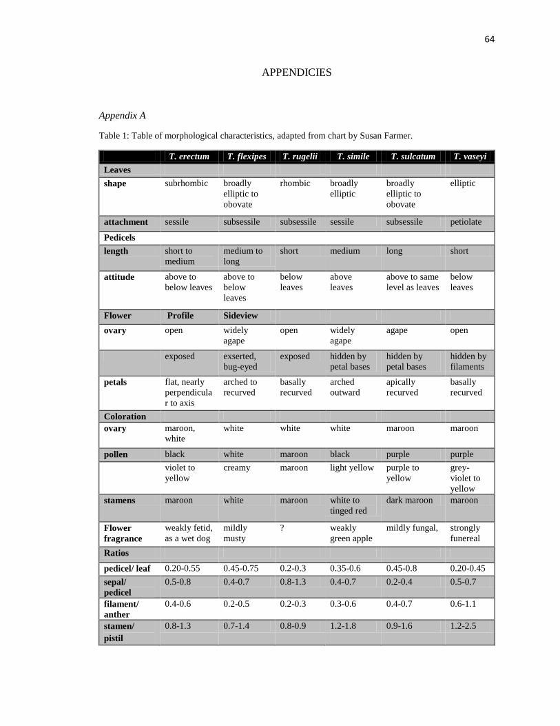
64

APPENDICIES

Appendix A

Table 1: Table of morphological characteristics, adapted from chart by Susan Farmer.

T. erectum T. flexipes T. rugelii T. simile T. sulcatum T. vaseyi

Leaves

shape subrhombic broadly

elliptic to

obovate

rhombic broadly

elliptic

broadly

elliptic to

obovate

elliptic

attachment sessile subsessile subsessile sessile subsessile petiolate

Pedicels

length short to

medium

medium to

long

short medium long short

attitude above to

below leaves

above to

below

leaves

below

leaves

above

leaves

above to same

level as leaves

below

leaves

Flower Profile Sideview

ovary open widely

agape

open widely

agape

agape open

exposed exserted,

bug-eyed

exposed hidden by

petal bases

hidden by

petal bases

hidden by

filaments

petals flat, nearly

perpendicula

r to axis

arched to

recurved

basally

recurved

arched

outward

apically

recurved

basally

recurved

Coloration

ovary maroon,

white

white white white maroon maroon

pollen black white maroon black purple purple

violet to

yellow

creamy maroon light yellow purple to

yellow

grey-

violet to

yellow

stamens maroon white maroon white to

tinged red

dark maroon maroon

Flower

fragrance

weakly fetid,

as a wet dog

mildly

musty

? weakly

green apple

mildly fungal, strongly

funereal

Ratios

pedicel/ leaf 0.20-0.55 0.45-0.75 0.2-0.3 0.35-0.6 0.45-0.8 0.20-0.45

sepal/

pedicel

0.5-0.8 0.4-0.7 0.8-1.3 0.4-0.7 0.2-0.4 0.5-0.7

filament/

anther

0.4-0.6 0.2-0.5 0.2-0.3 0.3-0.6 0.4-0.7 0.6-1.1

stamen/

pistil

0.8-1.3 0.7-1.4 0.8-0.9 1.2-1.8 0.9-1.6 1.2-2.5

65

Appendix B

Table 2: Pollination data

Color Taxa Number of

anthers dyed

Number of

anthers collected

Pollinated by

white flower

Pollinated by

red flower

White T. rugelii 28 15 11 4

Red

T. vaseyi 28 15 2 13

T. erectum 28 15 2 13

66

Appendix C

Table 3: Habitat characteristics extracted at known locations of individuals.

Species Geologic

Formation Forest Type

Avg.

Precip.

Avg.

Temp. Watershed

Soil

Type

erectum CZve Oak/Hickory Group 55 55 New 5153

erectum TRd Oak/Hickory Group 55 55 New 4858

erectum TRd Oak/Hickory Group 55 54 New 5769

erectum TRd Oak/Hickory Group 55 54 New 6136

erectum TRd Oak/Hickory Group 57 53 New 6757

erectum TRd Oak/Hickory Group 57 53 New 6552

erectum TRd Oak/Hickory Group 57 53 New 6582

erectum Mc Oak/Hickory Group 57 53 New 6582

erectum CZve Oak/Hickory Group 57 54 New 5897

erectum TRd Oak/Hickory Group 63 53 New 7733

erectum TRd Oak/Hickory Group 59 53 New 7032

erectum CZve Oak/Hickory Group 55 55 New 5153

erectum TRd Oak/Hickory Group 55 55 New 4858

erectum TRd Oak/Hickory Group 55 54 New 5769

erectum TRd Oak/Hickory Group 55 54 New 6136

erectum TRd Oak/Hickory Group 57 53 New 6757

erectum TRd Oak/Hickory Group 57 53 New 6552

erectum TRd Oak/Hickory Group 57 53 New 6582

erectum Mc Oak/Hickory Group 57 53 New 6582

erectum CZve Oak/Hickory Group 57 54 New 5897

erectum TRd Oak/Hickory Group 63 53 New 7733

erectum TRd Oak/Hickory Group 59 53 New 7032

erectum CZmv Oak/Hickory Group 69 50 New 4342

erectum PzZu Oak/Hickory Group 61 53 New 3384

erectum CZmv Oak/Hickory Group 69 50 New 4342

erectum CZmv Oak/Hickory Group 69 50 New 4342

erectum CZtp Oak/Hickory Group 55 55 New

erectum CZtp Oak/Hickory Group 55 55 New

erectum CZtp Oak/Hickory Group 69 50 New 2255

erectum CZmv Oak/Hickory Group 69 50 New 4342

erectum TRd Oak/Hickory Group 79 52 Savannah 12847

erectum TRd Oak/Hickory Group 77 52 Savannah 12826

erectum TRd Oak/Hickory Group 85 49 Savannah 13724

erectum TRd Maple/Beech/Birch 85 49 Savannah 13373

erectum TRd Oak/Hickory Group 67 49 Savannah 11307

erectum PzZu White/Red/Jack Pine 77 45 Savannah 806

erectum PzZg Oak/Hickory Group 65 48 New 462

erectum TRd Oak/Hickory Group 85 48 Savannah 13533

erectum TRd Oak/Hickory Group 81 50 Savannah 13723

erectum TRd Oak/Hickory Group 79 50 Savannah 3782

erectum PzZg Oak/Hickory Group 71 48 New 191

erectum PzZg Oak/Hickory Group 67 49 New 152

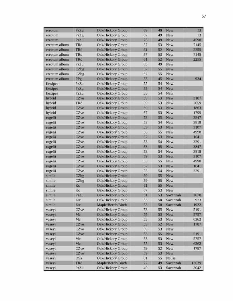
67

erectum PzZg Oak/Hickory Group 69 49 New 13

erectum PzZg Oak/Hickory Group 67 49 New 13

erectum PzZu Oak/Hickory Group 75 49 New 4590

erectum album TRd Oak/Hickory Group 57 53 New 7145

erectum album TRd Oak/Hickory Group 61 52 New 2255

erectum album TRd Oak/Hickory Group 57 53 New 7145

erectum album TRd Oak/Hickory Group 61 52 New 2255

erectum album PzZu Oak/Hickory Group 85 49 New

erectum album CZbg Oak/Hickory Group 57 55 New

erectum album CZbg Oak/Hickory Group 57 55 New

erectum album PPg Oak/Hickory Group 83 45 New 924

flexipes PzZu Oak/Hickory Group 55 54 New

flexipes PzZu Oak/Hickory Group 55 54 New

flexipes PzZu Oak/Hickory Group 55 54 New

hybrid CZve Oak/Hickory Group 59 53 New 3107

hybrid TRd Oak/Hickory Group 59 53 New 2059

hybrid CZve Oak/Hickory Group 59 53 New 1863

hybrid CZve Oak/Hickory Group 57 53 New 1799

rugelii CZve Oak/Hickory Group 53 55 New 3847

rugelii CZve Oak/Hickory Group 53 54 New 3818

rugelii CZve Oak/Hickory Group 59 53 New 3107

rugelii CZve Oak/Hickory Group 53 55 New 4998

rugelii CZve Oak/Hickory Group 57 53 New 1641

rugelii CZve Oak/Hickory Group 53 54 New 3291

rugelii CZve Oak/Hickory Group 53 55 New 3847

rugelii CZve Oak/Hickory Group 53 54 New 3818

rugelii CZve Oak/Hickory Group 59 53 New 3107

rugelii CZve Oak/Hickory Group 53 55 New 4998

rugelii CZve Oak/Hickory Group 57 53 New 1641

rugelii CZve Oak/Hickory Group 53 54 New 3291

simile CZbg Oak/Hickory Group 59 55 New

simile CZbg Oak/Hickory Group 59 55 New

simile Kc Oak/Hickory Group 61 55 New

simile Kc Oak/Hickory Group 67 53 New

simile PzZu Oak/Hickory Group 51 53 Savannah 2678

simile Zsr Oak/Hickory Group 53 50 Savannah 973

simile Zsr Maple/Beech/Birch 53 50 Savannah 1922

vaseyi CZve Oak/Hickory Group 53 55 New 5191

vaseyi Mc Oak/Hickory Group 55 53 New 5757

vaseyi Mc Oak/Hickory Group 55 53 New 6262

vaseyi CZve Oak/Hickory Group 59 52 New 1787

vaseyi CZve Oak/Hickory Group 59 53 New

vaseyi CZve Oak/Hickory Group 53 55 New 5191

vaseyi Mc Oak/Hickory Group 55 53 New 5757

vaseyi Mc Oak/Hickory Group 55 53 New 6262

vaseyi CZve Oak/Hickory Group 59 52 New 1787

vaseyi CZve Oak/Hickory Group 59 53 New

vaseyi DSs Oak/Hickory Group 81 55 Neuse

vaseyi TRd Maple/Beech/Birch 77 49 Savannah 13639

vaseyi PzZu Oak/Hickory Group 49 53 Savannah 3042

68

vaseyi Zsr Maple/Beech/Birch 53 50 Savannah 992

vaseyi TRd Oak/Hickory Group 49 51 Savannah 10956

vaseyi TRd Oak/Hickory Group 91 48 Savannah 13379

vaseyi Zsr Oak/Hickory Group 53 49 Savannah 1865

vaseyi Zb Oak/Hickory Group 65 55 New

vaseyi PzZu Oak/Hickory Group 55 54 New

69

Appendix D

Table 6: Allozyme trials. NR: not resolved

Enzyme Number of loci Number of alleles per locus

G-6PD 1 3

PGM 2 2

FE 1 NR

LAP NR NR

ATT 2 2-4

PGI NR NR

APER 1 2

MNR 1 6

CPER 2 2-4

UGPP 2 1-4

IDH 1 2

SKDH 1 5

DIA 1 4

TPI 2 2

Table 8: Genetic distance values from Allozyme data between taxa. A= T. erectum var.

album, E= T. erectum, V= T. vaseyi, R= T. rugelii, F= T. flexipes, SI= T. simile.

A E F R SI V Taxa

0.000 A

0.012 0.000 E

0.198 0.202 0.000 F

0.126 0.154 0.154 0.000 R

0.070 0.118 0.230 0.064 0.000 SI

0.026 0.040 0.240 0.219 0.133 0.000 V

Table 9: Genetic identity values from Allozyme data between taxa. A= T. erectum var.

album, E= T. erectum, V= T. vaseyi, R= T. rugelii, F= T. flexipes, SI= T. simile.

A E F R SI V Taxa

1.000 A

0.988 1.000 E

0.821 0.817 1.000 F

0.881 0.857 0.857 1.000 R

0.932 0.889 0.795 0.938 1.000 SI

0.974 0.960 0.786 0.804 0.876 1.000 V

70

Table 10: Pairwise Locality Matrix of Nei Unbiased Genetic Distance.

BMP WCU WFCK STIND WWF GSM FH BRM WWM MC OCO NG

0.000 BMP

0.397 0.000 WCU

0.500 0.642 0.000 WFCK

0.316 0.077 0.360 0.000 STIND

0.682 0.322 1.040 0.585 0.000 WWF

0.281 0.095 0.468 0.000 0.599 0.000 GSM

0.467 0.110 0.723 0.172 0.248 0.293 0.000 FH

0.529 0.162 0.848 0.324 0.010 0.326 0.141 0.000 BRM

0.534 0.218 0.699 0.334 0.027 0.314 0.308 0.007 0.000 WWM

0.454 0.138 0.725 0.377 0.097 0.338 0.224 0.072 0.057 0.000 MC

0.653 0.145 1.053 0.420 0.056 0.446 0.194 0.026 0.054 0.083 0.000 OCO

0.425 0.121 0.678 0.345 0.140 0.304 0.224 0.104 0.088 0.000 0.117 0.000 NG

0.705 0.180 1.067 0.550 0.043 0.586 0.181 0.048 0.100 0.054 0.041 0.073 RNBWF

Table 11: Pairwise Locality Matrix of Nei Unbiased Genetic Identity.

BMP WCU WFCK STIND WWF GSM FH BRM WWM MC OCO NG

1.000 BMP

0.673 1.000 WCU

0.607 0.526 1.000 WFCK

0.729 0.926 0.698 1.000 STIND

0.505 0.724 0.354 0.557 1.000 WWF

0.755 0.910 0.627 1.019 0.549 1.000 GSM

0.627 0.896 0.485 0.842 0.780 0.746 1.000 FH

0.589 0.851 0.428 0.723 0.990 0.722 0.869 1.000 BRM

0.586 0.804 0.497 0.716 0.973 0.730 0.735 0.993 1.000 WWM

0.635 0.871 0.485 0.686 0.908 0.713 0.799 0.930 0.945 1.000 MC

0.521 0.865 0.349 0.657 0.945 0.640 0.823 0.974 0.948 0.920 1.000 OCO

0.654 0.886 0.508 0.708 0.869 0.738 0.799 0.901 0.916 1.009 0.890 1.000 NG

0.494 0.835 0.344 0.577 0.958 0.557 0.835 0.953 0.905 0.947 0.960 0.929 RNBWF

Table 12: Summary AMOVA table by taxa.

Source df SS MS Est. Var. %

Among Taxa 5 63.541 12.708 0.319 10%

Within Taxa 192 567.333 2.955 2.955 90%

Total 197 630.874 3.274 100%

71

Table 13: Mean heterozygosity and standard error over all loci for each Locality

Pop Column1 Ho He

BMP Mean 0.125 0.219

SE 0.125 0.129

WCU Mean 0.331 0.468

SE 0.133 0.061

Wolf Creek Mean 0.250 0.250

SE 0.160 0.144

Standing Indian Mean 0.600 0.365

SE 0.216 0.124

WW Falls Mean 0.238 0.344

SE 0.085 0.099

GSMNP Mean 0.333 0.326

SE 0.152 0.111

Frozenhead Mean 0.176 0.253

SE 0.090 0.113

Black Rock Mtn Mean 0.343 0.495

SE 0.115 0.071

War Woman Mean 0.311 0.517

SE 0.030 0.040

Moses Creek Mean 0.413 0.341

SE 0.171 0.117

Oconolunftee Mean 0.352 0.487

SE 0.118 0.058

N GORGE Mean 0.375 0.307

SE 0.169 0.122

RAINBOW FALLS Mean 0.342 0.371

SE 0.123 0.077

Table 14: Mean Heterozygosity and SE over Loci for groups of Red and White Individuals.

Group Column1 Ho He

W Mean 0.347 0.484

SE 0.090 0.019

R Mean 0.329 0.483

SE 0.078 0.062

72

Table 15: Summary AMOVA table by locality and taxon.

Source df SS MS Est. Var. %

Among Regions 12 299.177 24.931 0.755 14%

Among Pops 12 114.884 9.574 1.092 20%

Within Pops 169 603.831 3.573 3.573 66%

Total 193 1017.892

5.420 100%

Table 16: Genetic distance matrix between three populations of T. vaseyi.

V-WWF V-BRM V-RF V-WWM

0.000 V-WWF

0.013 0.000 V-BRM

0.124 0.099 0.000 V-RF

0.021 0.005 0.127 0.000 V-WWM

Table 17: Summary of Chi-Square Tests for Hardy-Weinberg Equilibrium by Locality.

Key: ns=not significant, * P<0.05, ** P<0.01, *** P<0.001.

Pop Locus DF ChiSq Prob Signif

BMP UGPP 1 1 2.000 0.157 ns

BMP FE1 1 0.222 0.637 ns

BMP MNR 1 Monomorphic

BMP DIA 1 Monomorphic

WCU UGPP 1 3 23.037 0.000 ***

WCU FE1 6 28.107 0.000 ***

WCU MNR 1 1 2.798 0.094 ns

WCU DIA 1 3 0.600 0.896 ns

Wolf Creek UGPP 1 3 6.000 0.112 ns

Wolf Creek FE1 3 0.750 0.861 ns

Wolf Creek MNR 1 Monomorphic

Wolf Creek DIA 1 Monomorphic

Standing Indian UGPP 1 1 0.918 0.338 ns

Standing Indian FE1 3 2.222 0.528 ns

Standing Indian MNR 1 1 3.000 0.083 ns

Standing Indian DIA 1 Monomorphic

WW Falls UGPP 1 1 8.629 0.003 **

WW Falls FE1 1 2.333 0.127 ns

WW Falls MNR 1 1 1.976 0.160 ns

WW Falls DIA 1 3 2.794 0.424 ns

73

GSMNP UGPP 1 1 1.852 0.174 ns

GSMNP FE1 3 3.375 0.337 ns

GSMNP MNR 1 1 0.750 0.386 ns

GSMNP DIA 1 Monomorphic

Frozenhead UGPP 1 1 0.219 0.640 ns

Frozenhead FE1 1 6.516 0.011 *

Frozenhead MNR 1 Monomorphic

Frozenhead DIA 1 1 0.083 0.773 ns

Black Rock Mtn UGPP 1 1 7.783 0.005 **

Black Rock Mtn FE1 3 2.557 0.465 ns

Black Rock Mtn MNR 1 1 6.496 0.011 *

Black Rock Mtn DIA 1 6 5.031 0.540 ns

War Woman UGPP 1 3 3.953 0.267 ns

War Woman FE1 3 10.000 0.019 *

War Woman MNR 1 1 2.090 0.148 ns

War Woman DIA 1 3 6.366 0.095 ns

Moses Creek UGPP 1 Monomorphic

Moses Creek FE1 1 1.612 0.204 ns

Moses Creek MNR 1 1 10.164 0.001 **

Moses Creek DIA 1 3 2.051 0.562 ns

OCO UGPP 1 1 24.478 0.000 ***

OCO FE1 1 6.912 0.009 **

OCO MNR 1 1 3.789 0.052 ns

OCO DIA 1 3 15.264 0.002 **

N GORGE UGPP 1 Monomorphic

N GORGE FE1 3 1.106 0.776 ns

N GORGE MNR 1 1 7.200 0.007 **

N GORGE DIA 1 1 0.163 0.686 ns

RAINBOW FALLS UGPP 1 1 0.099 0.753 ns

RAINBOW FALLS FE1 3 1.837 0.607 ns

RAINBOW FALLS MNR 1 1 1.333 0.248 ns

RAINBOW FALLS DIA 1 1 6.368 0.012 *

74

Table 18: Summary of Chi-Square Tests for Hardy-Weinberg Equilibrium. Key: ns=not

significant, * P<0.05, ** P<0.01, *** P<0.001.

Pop Locus DF ChiSq Prob Signif

W UGPP 1 3 79.861 0.000 ***

W FE1 6 41.684 0.000 ***

W MNR 1 1 5.775 0.016 *

W DIA 1 6 28.375 0.000 ***

R UGPP 1 3 71.345 0.000 ***

R FE1 6 29.174 0.000 ***

R MNR 1 1 0.044 0.834 ns

R DIA 1 6 25.676 0.000 ***

Table 19: Allele frequencies by taxa. A= T. erectum var. album, E= T. erectum, V= T.

vaseyi, R= T. rugelii, F= T. flexipes, SI= T. simile.

Locus Allele/n A E F R SI V

UGPP1 N 53 24 9 20 23 67

2 0.009 0.063 0.000 0.025 0.000 0.052

3 0.179 0.188 0.667 0.475 0.370 0.157

4 0.811 0.750 0.333 0.500 0.630 0.791

FE1 N 49 21 11 17 23 65

2 0.031 0.048 0.000 0.118 0.000 0.054

3 0.439 0.548 0.227 0.059 0.283 0.431

4 0.531 0.405 0.773 0.735 0.696 0.485

5 0.000 0.000 0.000 0.088 0.022 0.031

MNR1 N 48 19 10 19 22 63

1 0.635 0.632 1.000 0.421 0.455 0.762

2 0.365 0.368 0.000 0.579 0.545 0.238

DIA1 N 45 22 10 12 18 61

1 0.256 0.273 0.000 0.125 0.139 0.451

2 0.633 0.727 1.000 0.792 0.500 0.451

3 0.100 0.000 0.000 0.083 0.361 0.074

4 0.011 0.000 0.000 0.000 0.000 0.025

75

Table 20: F-Statistics and Estimates of Nm over All Taxa for each Locus

All Pops. Locus Fis Fit Fst Nm

UGPP1 0.633 0.682 0.135 1.595

FE1 0.319 0.381 0.091 2.509

MNR1 -0.335 -0.114 0.166 1.257

DIA1 0.238 0.348 0.144 1.484

Mean 0.214 0.324 0.134 1.712

SE 0.202 0.164 0.016 0.275

Table 21: Summary of Chi-Square Tests for Hardy-Weinberg Equilibrium by Taxa. Key:

ns=not significant, * P<0.05, ** P<0.01, *** P<0.001.

Pop Locus DF ChiSq Prob Signif

E UGPP1 3 19.510 0.000 ***

E FE1 3 3.239 0.356 ns

E MNR1 1 4.321 0.038 *

E DIA1 1 0.617 0.432 ns

F UGPP1 1 0.000 1.000 ns

F FE1 1 6.043 0.014 *

F MNR1 1 0.139 0.709 ns

F DIA1 1 0.139 0.709 ns

R UGPP1 1 18.000 0.000 ***

R FE1 6 16.444 0.012 *

R MNR1 1 5.159 0.023 *

R DIA1 3 0.625 0.891 ns

SI UGPP1 1 18.908 0.000 ***

SI FE1 3 5.096 0.165 ns

SI MNR1 1 4.791 0.029 *

SI DIA1 3 4.698 0.195 ns

V UGPP1 3 44.799 0.000 ***

V FE1 6 23.935 0.001 ***

V MNR1 1 4.811 0.028 *

V DIA1 6 20.306 0.002 **

A UGPP1 3 19.577 0.000 ***

A FE1 3 1.095 0.778 ns

A MNR1 1 5.317 0.021 *

A DIA1 6 10.961 0.090 ns

76

Table 22: Mean Heterozygosity and SE over Loci for each taxa. A= T. erectum var.

album, E= T. erectum, V= T. vaseyi, R= T. rugelii, F= T. flexipes, SI= T. simile. Observed

heterozygosity= Ho; expected heterozygosity= He.

Pop Ho He

A Mean 0.401 0.455

SE 0.114 0.051

E Mean 0.364 0.449

SE 0.108 0.033

F Mean 0.134 0.199

SE 0.106 0.116

R Mean 0.374 0.449

SE 0.143 0.038

SI Mean 0.369 0.499

SE 0.145 0.036

V Mean 0.299 0.468

SE 0.073 0.066

Table 23: F-Statistics and Estimates of Nm over All Localities for each Locus

All Pops. Locus Fis Fit Fst Nm

UGPP 1 0.470 0.671 0.381 0.407

FE1 0.086 0.225 0.152 1.394

MNR 1 -0.310 0.294 0.461 0.292

DIA 1 0.247 0.456 0.276 0.654

Mean 0.123 0.412 0.318 0.687

SE 0.164 0.099 0.067 0.248

77

Table 24: Allele frequencies by locality.

Locus Allele BMP WCU Wolf

Creek

Standing

Indian

WW Falls GSMNP Frozenhead

UGPP 1 2 0.000 0.022 0.667 0.300 0.000 0.000 0.000

3 0.500 0.543 0.167 0.700 0.071 0.750 0.571

4 0.500 0.435 0.167 0.000 0.929 0.250 0.429

FE1 2 0.000 0.105 0.167 0.100 0.000 0.250 0.000

3 0.750 0.211 0.667 0.600 0.500 0.667 0.267

4 0.250 0.605 0.167 0.300 0.500 0.083 0.733

5 0.000 0.079 0.000 0.000 0.000 0.000 0.000

MNR 1 1 0.000 0.447 0.000 0.500 0.875 0.333 1.000

2 0.000 0.553 0.000 0.500 0.125 0.667 0.000

DIA 1 1 0.000 0.100 0.000 0.000 0.579 0.000 0.000

2 1.000 0.833 1.000 1.000 0.368 1.000 0.929

3 0.000 0.067 0.000 0.000 0.053 0.000 0.000

4 0.000 0.000 0.000 0.000 0.000 0.000 0.071

Locus Allele Black Rock

Mountain

War

Woman

Moses

Creek

Ocono Nantahala

Gorge

Rainbow Falls

UGPP 1 2 0.000 0.182 0.000 0.000 0.000 0.000

3 0.275 0.091 0.000 0.276 0.000 0.083

4 0.725 0.727 1.000 0.724 1.000 0.917

FE1 2 0.125 0.100 0.000 0.000 0.000 0.000

3 0.450 0.600 0.425 0.311 0.400 0.100

4 0.425 0.300 0.575 0.689 0.575 0.700

5 0.000 0.000 0.000 0.000 0.025 0.200

MNR 1 1 0.775 0.591 0.543 0.639 0.500 0.750

2 0.225 0.409 0.457 0.361 0.500 0.250

DIA 1 1 0.395 0.450 0.190 0.395 0.125 0.450

2 0.447 0.400 0.762 0.342 0.875 0.550

3 0.105 0.150 0.048 0.263 0.000 0.000

4 0.053 0.000 0.000 0.000 0.000 0.000

78

Table 25: Genetic identity matrix for three populations of T. vaseyi.

V-WWF V-BRM V-RF V-WWM

1.000 V-WWF

0.987 1.000 V-BRM

0.883 0.905 1.000 V-RF

0.979 0.995 0.881 1.000 V-WWM

Table 26: Allele Frequencies for three populations of T. vaseyi. N= sample size.

Locus Allele/n V-WWF V-BRM V-RF V-WWM

UGPP1 N 19 20 9 11

2 0.000 0.000 0.000 0.182

3 0.079 0.275 0.056 0.091

4 0.921 0.725 0.944 0.727

FE1 N 19 20 7 10

2 0.000 0.125 0.000 0.100

3 0.553 0.450 0.000 0.600

4 0.447 0.425 0.786 0.300

5 0.000 0.000 0.214 0.000

AAT1 N 16 16 8 7

3 0.219 0.375 0.063 0.214

4 0.750 0.625 0.875 0.786

5 0.031 0.000 0.063 0.000

MNR1 N 18 20 9 11

1 0.944 0.775 0.667 0.591

2 0.056 0.225 0.333 0.409

MNR2 N 17 16 2 8

1 0.971 0.875 0.500 0.938

2 0.029 0.125 0.500 0.063

DIA1 N 18 19 7 10

1 0.611 0.395 0.357 0.450

2 0.333 0.447 0.643 0.400

3 0.056 0.105 0.000 0.150

79

Table 27: Allele frequencies for red and white forms of Trillium at Clingman’s Dome.

Pop Allele/n UGPP1 FE1 DIA MNR1

Red flowered 1 0.500

2 0.000 0.000 0.250 0.500

3 0.000 0.500 0.500

4 1.000 0.500 0.250

White flowered 1 0.500

2 0.000 0.000 0.000 0.500

3 0.000 0.167 0.333

4 1.000 0.833 0.667

Table 28: Summary of AMOVA by locality.

Source df SS MS Est. Var. %

Among Pops 12 158.447 13.204 0.714 22%

Within Pops 187 486.453 2.601 2.601 78%

Total 199 644.900 3.315 100%

80

Appendix E

Table 29: Leaf tissue collections

Locality Species Quantity

Wolf Creek T. erectum 9

Black Rock Mtn T. vaseyi 26

Balsam Mountain Preserve T.erectum var. album 1

Balsam Mountain Preserve T. erectum 3

Balsam Mountain Preserve T. rugelii 2

Frozen Head T. flexipes 11

Frozen Head T. erectum 4

Frozen Head T. vaseyi 2

GSMNP T. erectum 9

GSMNP T. erectum var. album 8

GSMNP T.erectum hybrid 2

GSMNP T. simile 11

GSMNP T. vaseyi 15

Moses Creek T. rugelii 4

Moses Creek T. erectum hybrid 8

Moses Creek T. erectum 6

Moses Creek T.erectum var. album 7

Nantahala Gorge T. simile 18

Nantahala Gorge T. album 3

Standing Indian T. erectum 3

Standing Indian T. erectum var. album 6

Standing Indian T. erectum hybrid 2

War Woman T. vaseyi 18

WCU T. rugelii 17

WCU T. rugelii hybrid 2

Whitewater Falls T. vaseyi 25

Whitewater Falls T. vaseyi (white flowered) 2

Oconolunftee T. erectum var. album 19

Oconolunftee T. simile 3

Oconolunftee T. vaseyi 2

Oconolunftee T. vaseyi hybrid 1

81

Table 7: Allozyme data set. N/A: individual not run for that locus, 99: not resolved.

Location Collection

number

UGPP

1 FE1 AAT1 MNR1 MNR2

DIA

1

BMP 1 33 33 N/A 99 N/A 22

BMP 3 44 34 N/A 99 N/A 22

WCU 8 33 99 N/A 99 N/A 99

WCU 11 33 44 N/A 22 N/A 99

WCU 13 33 22 N/A 22 N/A 22

WCU 15 33 22 N/A 12 N/A 99

WCU 16 33 99 N/A 99 N/A 99

WCU 17 33 44 N/A 12 N/A 99

WCU 18 33 44 N/A 22 N/A 99

WCU 19 33 44 N/A 12 N/A 22

WCU 20 33 99 N/A 12 N/A 22

WCU 21 33 44 N/A 12 N/A 99

Wolf Creek 24 22 23 N/A 99 N/A 22

Wolf Creek 30 34 33 N/A 99 N/A 22

Wolf Creek 31 22 34 N/A 99 N/A 22

Standing Indian 39 33 33 N/A 12 N/A 22

Standing Indian 40 23 34 N/A 99 N/A 22

Standing Indian 41 23 34 N/A 12 N/A 22

Standing Indian 42 33 23 N/A 12 N/A 22

Standing Indian 45 23 34 N/A 99 N/A 22

Whitewater Falls 48 44 33 33 11 11 13

82

Whitewater Falls 49 44 34 44 11 11 13

Whitewater Falls 50 34 33 99 11 11 11

Whitewater Falls 51 44 34 34 11 11 11

Whitewater Falls 52 44 44 44 12 12 11

Whitewater Falls 53 33 33 N/A 11 N/A 22

Whitewater Falls 54 44 44 N/A 99 N/A 22

Whitewater Falls 57 44 34 44 11 11 11

Whitewater Falls 59 44 44 44 12 11 11

Whitewater Falls 60 44 33 44 11 11 11

Whitewater Falls 63 44 33 44 11 11 22

Whitewater Falls 64 44 33 34 11 11 12

Whitewater Falls 66 44 34 45 11 11 12

Whitewater Falls 67 44 34 34 11 11 99

Whitewater Falls 68 44 44 44 11 11 11

Whitewater Falls 69 44 33 44 11 11 12

Whitewater Falls 70 44 44 34 11 11 12

Whitewater Falls 71 44 34 44 11 11 12

Whitewater Falls 72 44 34 34 11 11 12

GSMNP 93 44 33 N/A 99 N/A 22

GSMNP 106 33 23 N/A 12 N/A 22

GSMNP 108 33 23 N/A 99 N/A 22

GSMNP 109 33 33 N/A 12 N/A 22

GSMNP 113 33 33 N/A 99 N/A 22

GSMNP 115 34 24 N/A 22 N/A 22

83

Frozen Head 115 44 99 N/A 99 N/A 22

Frozen Head 117 33 34 N/A 99 N/A 22

Frozen Head 118 44 33 99 11 11 99

Frozen Head 120 33 44 N/A 11 N/A 22

Frozen Head 121 33 44 N/A 11 N/A 22

Frozen Head 122 33 44 N/A 11 N/A 22

Frozen Head 123 99 44 N/A 11 N/A 22

Frozen Head 124 34 44 N/A 11 N/A 22

Frozen Head 131 34 33 44 11 11 22

Frozen Head 132 44 34 44 11 11 99

Frozen Head 133 99 33 N/A 99 N/A 22

Frozen Head 134 34 44 N/A 11 N/A 22

Frozen Head 135 34 44 N/A 11 N/A 22

Black Rock Mtn 136 44 44 44 11 11 14

Frozen Head 136 33 44 N/A 11 N/A 22

Black Rock Mtn 137 44 34 44 11 11 33

Frozen Head 137 34 44 N/A 11 N/A 24

Black Rock Mtn 138 44 44 34 11 11 11

Frozen Head 138 34 44 N/A 11 N/A 24

Black Rock Mtn 139 33 23 N/A 22 N/A 99

Black Rock Mtn 140 33 24 N/A 22 N/A 22

Black Rock Mtn 142 34 34 34 11 11 24

Black Rock Mtn 146 44 44 33 11 11 13

Black Rock Mtn 147 44 33 34 11 11 12

84

Black Rock Mtn 148 44 33 34 11 11 22

Black Rock Mtn 149 44 33 44 11 11 22

Black Rock Mtn 150 34 34 34 22 22 23

Black Rock Mtn 151 44 34 44 11 11 12

Black Rock Mtn 152 34 34 44 11 11 11

Black Rock Mtn 153 44 34 44 11 11 12

Black Rock Mtn 154 44 34 33 12 12 12

Black Rock Mtn 156 44 33 34 12 12 12

Black Rock Mtn 157 33 22 N/A 11 N/A 22

Black Rock Mtn 158 33 24 N/A 12 N/A 22

Black Rock Mtn 159 44 34 44 11 11 11

Black Rock Mtn 160 44 34 33 11 11 11

War Woman 162 22 99 N/A 22 N/A 22

War Woman 163 44 34 44 11 11 12

War Woman 165 44 33 34 11 11 99

War Woman 166 24 22 N/A 22 N/A 22

War Woman 168 23 44 N/A 22 N/A 22

War Woman 169 44 33 44 11 11 12

War Woman 171 44 33 44 12 11 11

War Woman 172 44 34 99 11 11 33

War Woman 173 44 34 44 12 12 13

War Woman 174 44 34 44 12 11 11

War Woman 176 34 33 33 11 11 11

Moses Creek 220 44 34 33 12 12 23

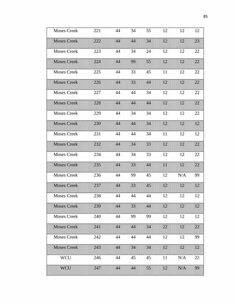
85

Moses Creek 221 44 34 55 12 12 12

Moses Creek 222 44 44 34 12 12 23

Moses Creek 223 44 34 24 12 12 22

Moses Creek 224 44 99 55 12 12 22

Moses Creek 225 44 33 45 11 12 22

Moses Creek 226 44 33 44 12 12 22

Moses Creek 227 44 44 34 12 12 22

Moses Creek 228 44 44 44 12 12 22

Moses Creek 229 44 34 34 12 12 22

Moses Creek 230 44 44 34 12 12 12

Moses Creek 231 44 44 34 11 12 12

Moses Creek 232 44 34 33 12 12 22

Moses Creek 234 44 34 33 12 12 22

Moses Creek 235 44 33 44 11 12 22

Moses Creek 236 44 99 45 12 N/A 99

Moses Creek 237 44 33 45 12 12 12

Moses Creek 238 44 44 44 12 12 12

Moses Creek 239 44 33 44 12 12 12

Moses Creek 240 44 99 99 12 12 12

Moses Creek 241 44 44 34 22 12 22

Moses Creek 242 44 44 44 12 12 99

Moses Creek 243 44 34 34 12 12 12

WCU 246 44 45 45 11 N/A 22

WCU 247 44 44 55 12 N/A 99

86

WCU 248 44 34 45 12 N/A 12

WCU 249 44 45 55 12 N/A 12

WCU 250 44 44 55 12 N/A 23

WCU 251 44 45 45 12 N/A 12

WCU 253 44 44 44 12 N/A 22

WCU 254 44 44 55 12 N/A 22

WCU 255 44 34 55 22 N/A 23

Oconaluftee 270 44 34 34 12 11 12

Oconaluftee 271 44 34 44 12 12 23

Oconaluftee 272 44 44 34 12 11 11

Oconaluftee 273 44 33 44 11 12 12

Oconaluftee 274 44 44 44 11 12 11

Oconaluftee 275 34 33 33 12 12 22

Oconaluftee 276 44 44 44 12 12 23

Oconaluftee 277 44 44 34 12 11 11

Oconaluftee 278 44 33 34 11 12 12

Oconaluftee 279 44 34 44 11 11 11

Oconaluftee 280 44 34 34 11 12 12

Oconaluftee 281 44 33 34 11 11 12

Oconaluftee 282 44 34 44 11 12 33

Oconaluftee 283 44 34 33 12 12 12

Oconaluftee 284 44 33 34 11 11 11

Oconaluftee 285 44 34 23 12 12 12

Oconaluftee 286 44 44 34 12 99 12

87

Oconaluftee 287 44 99 55 12 99 22

Oconaluftee 288 44 34 34 12 99 22

Oconaluftee 290 44 33 34 11 11 12

Oconaluftee 291 34 44 34 11 11 23

Oconaluftee 292 44 44 23 11 12 12

Oconaluftee 293 44 44 44 12 12 11

Oconaluftee 294 44 34 44 12 12 11

Oconaluftee 295 44 44 44 12 22 11

Oconaluftee 296 44 33 44 11 11 11

Oconaluftee 297 44 44 99 12 12 22

Oconaluftee 298 44 44 44 12 11 11

Nantahala Gorge 300 44 34 34 12 12 99

Nantahala Gorge 301 44 34 99 12 11 99

Nantahala Gorge 301 44 44 34 12 12 99

Nantahala Gorge 303 44 34 44 12 12 22

Nantahala Gorge 304 44 34 44 12 99 99

Nantahala Gorge 305 44 45 44 12 12 99

Nantahala Gorge 306 44 34 34 12 12 12

Nantahala Gorge 309 44 44 33 12 12 99

Nantahala Gorge 308 44 34 99 22 12 22

Nantahala Gorge 309 44 33 34 12 12 99

Nantahala Gorge 310 44 33 33 22 12 22

Nantahala Gorge 312 44 44 34 12 12 22

Nantahala Gorge 313 44 44 34 11 12 99

88

Nantahala Gorge 314 44 34 44 12 12 12

Nantahala Gorge 315 44 33 44 12 12 22

Nantahala Gorge 316 44 34 99 12 11 99

Nantahala Gorge 317 44 33 34 12 11 99

Nantahala Gorge 318 44 44 34 12 12 99

Nantahala Gorge 322 44 44 99 11 11 99

Nantahala Gorge 323 44 44 34 12 12 22

Rainbow Falls 330 34 34 34 11 11 11

Rainbow Falls 331 44 34 44 11 11 11

Rainbow Falls 332 44 45 44 11 N/A 22

Rainbow Falls 334 44 44 44 11 12 11

Rainbow Falls 335 44 99 45 12 N/A 22

Rainbow Falls 336 44 44 34 12 N/A 99

Rainbow Falls 337 44 44 44 11 12 11

Rainbow Falls 338 44 44 44 12 N/A 99

Rainbow Falls 339 44 45 44 11 N/A 22

Rainbow Falls 340 44 45 44 12 N/A 22

Rainbow Falls 341 44 45 99 12 N/A 12

Rainbow Falls 342 34 99 44 12 N/A 22

Whitewater Falls 350 44 44 44 22 N/A 99

Whitewater Falls 351 44 44 44 12 N/A 22

WCU A-maroon

thecae 23 99 N/A 12 N/A 22

Oconaluftee 202 34 44 N/A 22 N/A 33

89

Oconaluftee 203 33 44 N/A 22 N/A 33

Oconaluftee 204 33 44 N/A 12 N/A 23

Oconaluftee 205 33 44 N/A 12 N/A 23

Oconaluftee 206 33 44 N/A 99 N/A 33

Oconaluftee 207 33 44 N/A 12 N/A 23

Oconaluftee 208 33 44 N/A 12 N/A 33

Oconaluftee 209 33 44 N/A 12 N/A 23

Oconaluftee 210 33 44 N/A 12 N/A 23

Oconaluftee 211 33 44 N/A 12 N/A 33

WCU A-yellow

thecae 33 33 N/A 11 N/A 22