A Study of Skills, Problem Solving, andCollaboration Networks

by

Katharine A. Anderson

A dissertation submitted in partial fulfillmentof the requirements for the degree of

Doctor of Philosophy(Economics)

in The University of Michigan2010

Doctoral Committee:

Professor Scott E. Page, ChairProfessor Robert WillisAssistant Professor Lada AdamicAssistant Professor Stephan Lauermann

c© Katharine A. Anderson 2010

All Rights Reserved

ACKNOWLEDGEMENTS

I first express my gratitude to my advisor, Scott Page, who has been a true mentor.

Thanks also to Lada Adamic, Rick Riolo, Dan Silverman, Bob Willis, Kai-Uwe

Kuhn, Steve Salant, Charlie Brown, Yusufcan Masatlioglu, and Stephan Lauermann

who have been so generous with their time. Thanks to the membership of the Complex

Systems Advanced Academic Workshop, which has been the earliest audience for

much of my work. Thanks also to Ross O’Connell, who is both my harshest and best

critic.

This work has been funded, in part, by the National Science Foundation. The

Center for the Study of Complex Systems has provided me with computing resources,

and (more importantly) an academic home.

There are many people who have gotten me here in one piece. Thank you to the

physics cronies, the members of Lorch 107, and the Grinnell Plans community. I also

thank my parents and sister, who delivered me to adulthood. Finally, I thank my

Nora, who made my life interesting near the end of this process, and my dearest Ross,

who makes me whole.

ii

TABLE OF CONTENTS

ACKNOWLEDGEMENTS . . . . . . . . . . . . . . . . . . . . . . . . . . ii

LIST OF FIGURES . . . . . . . . . . . . . . . . . . . . . . . . . . . . . . . vi

LIST OF TABLES . . . . . . . . . . . . . . . . . . . . . . . . . . . . . . . . xii

LIST OF APPENDICES . . . . . . . . . . . . . . . . . . . . . . . . . . . . xiii

ABSTRACT . . . . . . . . . . . . . . . . . . . . . . . . . . . . . . . . . . . xiv

CHAPTER

I. Introduction . . . . . . . . . . . . . . . . . . . . . . . . . . . . . . 1

1.1 Collaborative Problem Solving and Innovation . . . . . . . . 31.1.1 Team Assembly . . . . . . . . . . . . . . . . . . . . 41.1.2 Agent Heterogeneity . . . . . . . . . . . . . . . . . . 51.1.3 Skill Acquisition . . . . . . . . . . . . . . . . . . . . 6

1.2 Network Structure and Behavior . . . . . . . . . . . . . . . . 61.2.1 Introduction to some relevant network concepts . . 71.2.2 The structure and function of social networks . . . . 7

1.3 Overview of this thesis . . . . . . . . . . . . . . . . . . . . . . 11

II. Collaboration Network Formation and the Demand for Knowl-edge Workers with Heterogeneous Skills . . . . . . . . . . . . . 12

2.1 Introduction . . . . . . . . . . . . . . . . . . . . . . . . . . . 122.2 A General Model of Skills, Problem Solving, and Collaboration

Networks . . . . . . . . . . . . . . . . . . . . . . . . . . . . . 192.2.1 Inputs: Problem Solving Population and Problems . 192.2.2 Cost-minimizing Collaboration Networks . . . . . . 222.2.3 Example . . . . . . . . . . . . . . . . . . . . . . . . 232.2.4 Discussion . . . . . . . . . . . . . . . . . . . . . . . 23

iii

2.2.5 A Note on Stability and Efficiency of the Cost Mini-mizing Social Network . . . . . . . . . . . . . . . . 25

2.3 Skills and Degree: Skill Sets and Collaborative Success . . . . 262.3.1 Skills and Degree: An Example . . . . . . . . . . . 262.3.2 Skills and Degree: General Results . . . . . . . . . . 272.3.3 Bundled Skills and the Importance of Skill Combina-

tions . . . . . . . . . . . . . . . . . . . . . . . . . . 292.4 Skill Distributions and the Distribution of Prominence: The

Bernoulli Skills Model . . . . . . . . . . . . . . . . . . . . . . 322.4.1 The Bernoulli Skills Model . . . . . . . . . . . . . . 322.4.2 Degree Distribution of the Bernoulli Skills Model . . 332.4.3 Problem Difficulty and the Distribution of Degree . 38

2.5 Skill Ladders: Specialization and Degree . . . . . . . . . . . . 412.5.1 Notation and Definitions . . . . . . . . . . . . . . . 412.5.2 Example: a single ladder of skills . . . . . . . . . . . 432.5.3 Results for m ladders . . . . . . . . . . . . . . . . . 44

2.6 A Comparison to a Model with a Single Skill . . . . . . . . . 472.7 Implications: Labor Markets and Industrial Organization . . 51

2.7.1 Extending the Model to Employment by Firms . . . 512.7.2 Returns to Skills and Optimal Training Decisions . 522.7.3 Variation in Labor Demand . . . . . . . . . . . . . . 532.7.4 Industrial Organization . . . . . . . . . . . . . . . . 55

2.8 Extensions . . . . . . . . . . . . . . . . . . . . . . . . . . . . 562.8.1 Bargaining Over Surplus . . . . . . . . . . . . . . . 562.8.2 Long Run Skill Acquisition . . . . . . . . . . . . . . 57

2.9 Conclusion . . . . . . . . . . . . . . . . . . . . . . . . . . . . 58

III. Foxes and Hedgehogs: Equilibrium Skill Acquisition Deci-sions in Problem-solving Populations . . . . . . . . . . . . . . . 60

3.1 Introduction . . . . . . . . . . . . . . . . . . . . . . . . . . . 603.2 Model . . . . . . . . . . . . . . . . . . . . . . . . . . . . . . . 623.3 Results: Specialization and Barriers Between Disciplines . . . 65

3.3.1 A Special Case: Symmetry Across Disciplines . . . . 653.3.2 Optimality of the Equilibrium . . . . . . . . . . . . 683.3.3 Discussion . . . . . . . . . . . . . . . . . . . . . . . 71

3.4 An Extension: Problems with Multiple Parts . . . . . . . . . 723.4.1 Problems With Multiple Parts . . . . . . . . . . . . 72

3.5 Conclusion . . . . . . . . . . . . . . . . . . . . . . . . . . . . 77

IV. Team Assembly with Network Constraints . . . . . . . . . . . 79

4.1 Introduction . . . . . . . . . . . . . . . . . . . . . . . . . . . 794.2 Basic Model Elements and the Static Game . . . . . . . . . . 83

4.2.1 Static Group Formation Game . . . . . . . . . . . . 85

iv

4.3 Sequential Group Formation Game–The Unconstrained Case 914.3.1 Sequential Coalition Formation Game . . . . . . . . 914.3.2 Discussion–Externalities in Coalition Membership . 96

4.4 Sequential Group Formation with a Network Constraint . . . 984.4.1 The Static Game–Network Constraints and Variable

Group Size . . . . . . . . . . . . . . . . . . . . . . . 1004.4.2 The Sequential Game–Network Topology and Effi-

ciency . . . . . . . . . . . . . . . . . . . . . . . . . 1034.5 The Effects of Network Topology on Optimal Institutional Design1074.6 Extensions and conclusions . . . . . . . . . . . . . . . . . . . 108

V. Conclusion and Extensions . . . . . . . . . . . . . . . . . . . . . 115

APPENDICES . . . . . . . . . . . . . . . . . . . . . . . . . . . . . . . . . . 119

BIBLIOGRAPHY . . . . . . . . . . . . . . . . . . . . . . . . . . . . . . . . 136

v

LIST OF FIGURES

Figure

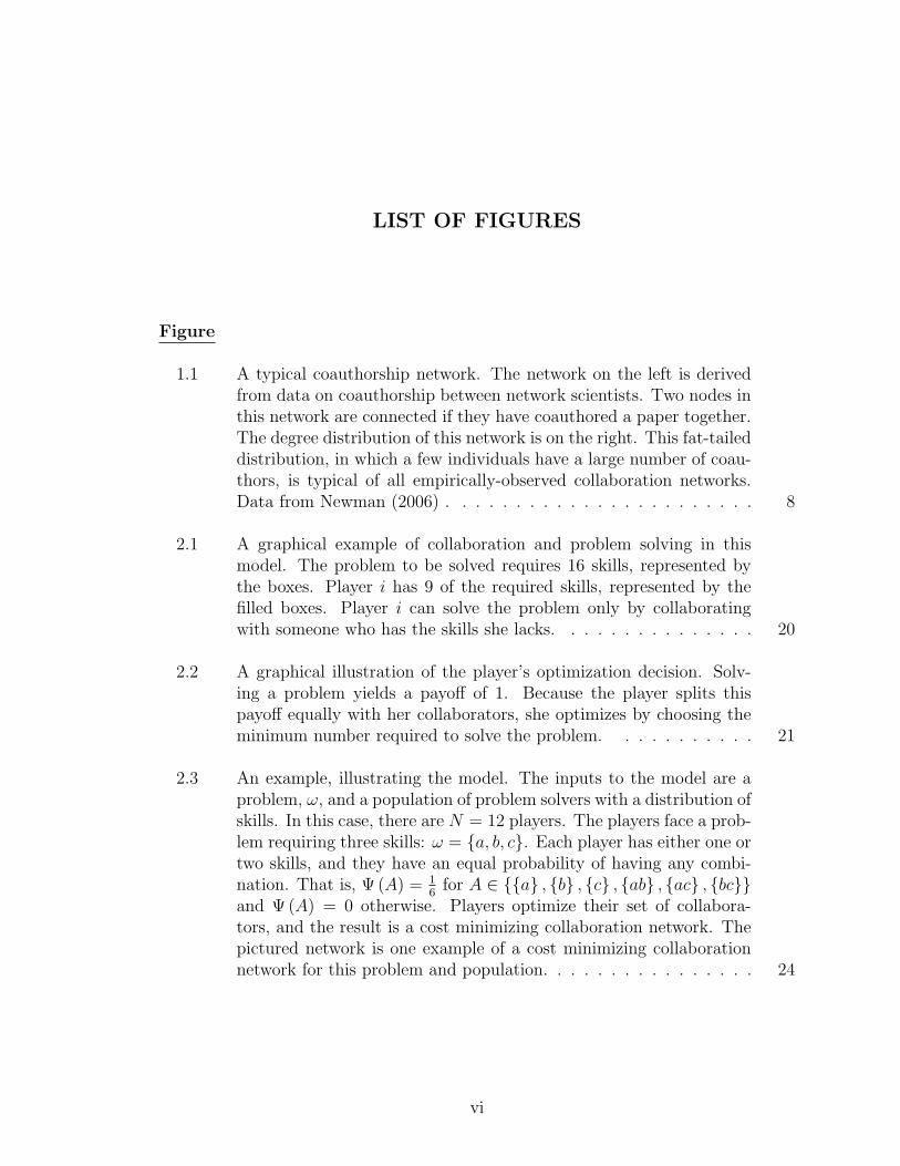
1.1 A typical coauthorship network. The network on the left is derivedfrom data on coauthorship between network scientists. Two nodes inthis network are connected if they have coauthored a paper together.The degree distribution of this network is on the right. This fat-taileddistribution, in which a few individuals have a large number of coau-thors, is typical of all empirically-observed collaboration networks.Data from Newman (2006) . . . . . . . . . . . . . . . . . . . . . . . 8

2.1 A graphical example of collaboration and problem solving in thismodel. The problem to be solved requires 16 skills, represented bythe boxes. Player i has 9 of the required skills, represented by thefilled boxes. Player i can solve the problem only by collaboratingwith someone who has the skills she lacks. . . . . . . . . . . . . . . 20

2.2 A graphical illustration of the player’s optimization decision. Solv-ing a problem yields a payoff of 1. Because the player splits thispayoff equally with her collaborators, she optimizes by choosing theminimum number required to solve the problem. . . . . . . . . . . 21

2.3 An example, illustrating the model. The inputs to the model are aproblem, ω, and a population of problem solvers with a distribution ofskills. In this case, there are N = 12 players. The players face a prob-lem requiring three skills: ω = a, b, c. Each player has either one ortwo skills, and they have an equal probability of having any combi-nation. That is, Ψ (A) = 1

6for A ∈ a , b , c , ab , ac , bc

and Ψ (A) = 0 otherwise. Players optimize their set of collabora-tors, and the result is a cost minimizing collaboration network. Thepictured network is one example of a cost minimizing collaborationnetwork for this problem and population. . . . . . . . . . . . . . . . 24

vi

2.4 In the Bernoulli Skills Model, a player’s degree is increasing in the sizeof her set of skills. The supermodularity of degree means that playerswith more skills receive many more links. This exaggerates any initialinequalities in the size of the skill sets. The resulting network has avery distinctive structure–a small number of players participate in amajority of the collaborations. . . . . . . . . . . . . . . . . . . . . . 36

2.5 Empirically, most collaboration networks have a skewed degree dis-tribution. The left panel depicts a coauthorship network for networkscientists–two nodes in this network are connected if the scientistscoauthored a paper together (only the largest connected componentis shown here). The right panel depicts the degree distribution forthis network. . . . . . . . . . . . . . . . . . . . . . . . . . . . . . . . 37

2.6 An example of the Gini coefficient for a discrete distribution, ∆ (y).In this case, the random variable y takes on one of five values, y0...y4.The Gini coefficient is the area of the shaded region between the lineof equality and the Lorenz curve. . . . . . . . . . . . . . . . . . . . 39

2.7 A graph of the Gini coefficient, G (p,M), for different populations.The four curves pictured represent different values of M , and the xaxis represents the value of p. The difficulty of a problem rises asthe number of skills required increases or the probability of having aparticular skill falls. . . . . . . . . . . . . . . . . . . . . . . . . . . . 40

2.8 A ladder of 6 skills–a player with skill ai in this set must have all ofthe skills that precede it: a1...ai−1. . . . . . . . . . . . . . . . . . . 42

2.9 An example of 12 skills arranged into four ladders of equal length. . 42

2.10 Two collaboration networks with 27 players. In both cases, the play-ers are solving a problem requiring M = 3 skills. These networksrepresent the two ends of a spectrum of skill specialization, withm = M ladders on the left and m = 1 ladders on the right. . . . . 44

2.11 The gini coefficient for M = 10, divided into different sets of ladders.The bottom curve pictures the case where m = 10, the second curvepictures the case where m = 5, the third shows m = 2, and the fourthshows m = 1. . . . . . . . . . . . . . . . . . . . . . . . . . . . . . . 46

vii

2.12 Contrasting the structure of collaboration networks resulting fromtype-based and skill-based models of collaboration. In both cases,the problem faced requires three skills. In the network on the left,each player has a single skill. In the network on the right, the threeskills are distributed independently with probability p = 1

3. The

bottom panels show both the distribution of degree in the picturednetworks (black dots) and the distribution of expected degree in theset of cost minimizing networks (grey bars). . . . . . . . . . . . . . 49

3.1 Two disciplines, each with three skills. . . . . . . . . . . . . . . . . 63

3.2 The equilibrium skill acquisition decisions as a function of the fractionof problems assigned to discipline 1 in the case where skills are sym-metric across disciplines (that is, where δ1 = δ2 = δ). If enough prob-lems are assigned to one of the disciplines, then all players will special-ize in that discipline. If problems are more evenly distributed acrossdisciplines, than players will tend to generalize. The point at whichindividuals will start to generalize depends on π = δh+ (1− δ) l, theexpected probability that a single skill will not solve the problem. . 68

3.3 Regions of social suboptimality. The line shows values of the param-eter φ–the fraction of problems assigned to discipline 1. The top partof the figure shows the parameter regions where individuals decide tospecialize. The bottom part of the figure shows where specializationis optimal from a societal perspective. The shaded areas indicate theparameter values where individuals choose to specialize, but societywould prefer to have at least a few generalists. . . . . . . . . . . . 69

3.4 A taxonomy of problem distributions. In the above, each problem

has two parts. The matrix

[δ11 δ21

δ12 δ22

]represents the distribution of

problems, where δid is the probability of a skill in discipline d beingan H skill for part i of the problem. In this case, I have simplifiedthe problem distributions by assuming that either δid = X (highprobability that the discipline will be useful on part i) or δid = O(low probability that the discipline will be useful on part i). Theproblem distributions can be divided into three categories accordingto which disciplines are more useful on which parts of the problem. 74

viii

3.5 Equilibrium decisions to specialize and generalize when problemshave two parts. The boundry between the regions where individ-uals specialize and generalize is defined by the equation πK1 + πK0 =

(π1π0)K−c

2 −(π1π0)K−c+(π1π0)K . This graph illustrates these regionsin the case where K = 3 and c = 1. This boundry moves upwards ascosts (c) rise, relative to a problem solver’s capacity (M = K + c). 76

4.1 An illustration of g –the smallest g such that f(g + 1) < f(2). . . . 85

4.2 Individual payoff function for Example IV.1. Note that the playersenjoy the highest payoff in a coalition of size 10. . . . . . . . . . . 89

4.3 The first individual to move joins another individual to form a groupof size 2. . . . . . . . . . . . . . . . . . . . . . . . . . . . . . . . . . 95

4.4 The second individual to move must choose between forming a newgroup of size 2 or joining the existing group of 3. He will choose thegroup of 3, since it gives him higher utility than the group of 2. . . 96

4.5 A new group forms when the large group is size g = 17 because theindividual is better off in a new group of size 2. . . . . . . . . . . . 97

4.6 A game with 12 players arranged on a ring. . . . . . . . . . . . . . . 101

4.7 An example of an equilibrium group configuration on a ring. Notethat this would not be an equilibrium on the fully-connected networkbecause the players in group C would move group A. . . . . . . . . 102

4.8 Four different networks connecting 12 players. Degree of the networkdecreases from left to right. The first panel depicts a fully connectednetwork. As edges are removed at random, average degree declinesand players potentially become more constrained in their choice ofgroups. . . . . . . . . . . . . . . . . . . . . . . . . . . . . . . . . . 104

4.9 Three different networks connecting 12 players. In the first panel,the players are connected to their two nearest neighbors on each side.This is called a regular network, and is often used to represent ar-rangements of individuals in space. In the second panel, a smallnumber of the links in the regular network are rewired at random.The result is called a small world network, and is a simple model ofa social network. In the last panel, all of the links in the originalnetwork are rewired at random. The result is a random network,similar to those depicted in Figure 4.8. Random networks are easilyanalyzed, but a poor approximation of social connections. . . . . . . 105

ix

4.10 Define efficiency to be ratio of actual social welfare to the maximumpossible social welfare. This plot shows average efficiency over 100runs of a sequential coalition formation game with N = 100 andf(g) = g(20−g). The network constraints are random (p = 1). As thedegree of the network constraint decreases, social welfare increases.Social welfare increases because the constraint binds more heavily,mitigating the tendency for groups to get too large. . . . . . . . . . 110

4.11 Define efficiency to be ratio of actual social welfare to the maximumpossible social welfare. This plot shows average efficiency for 100runs of a sequential coalition formation game. For all runs, N = 100and f(g) = g(20 − g). Holding degree constant (at 2, 4, 6) averagesocial welfare declines in the Watts-Strogatz parameter–that is, socialwelfare is higher when the network is ordered than when it is random. 111

4.12 An example in which the Exclusive Membership Rule induces a pooroutcome. In this game, g∗ = 3. If groups are able to deny member-ship, there is a possibility that more central individuals will form onegroup, leaving the outliers to a poor payoff. This degree distributionof this network is that of a hierarchical social structure. . . . . . . . 112

4.13 An example illustrating how the Exclusive Membership Rule can bedetrimental on a ring. This is a game with 20 individuals arrangedon a ring and g∗ = 3. Because the large groups can prevent themfrom joining, the isolated individuals must accept a lower payoff. . . 112

4.14 Comparing the exclusive membership rule to the open membershiprule for network constraints of different degree. . . . . . . . . . . . . 113

4.15 Comparing the exclusive membership rule to the open membershiprule for network constraints with different Watts-Strogatz parameters. 114

E.1 In this game, 12 individuals are arranged in a ring. The payoff func-tion, f(g), has maximum g∗ = 2 and g = 6. The individuals move inorder around the ring–φ1 = 1, 2, 3, 4, 5, 6, 7, 8, 9, 10, 11, 12–and windup in two groups of size 6. In fact, 〈6, 6〉 is the only equilibriumgroup size configuration of the game (12, f(g), φ1). Figure E.3 showsthe same game with a different order of play. . . . . . . . . . . . . . 132

E.2 An example of an equilibrium on fully-connected network. Wheng∗ = 3 and g = 6, Theorem 26 suggests that the individuals will forminto two groups of size 6. . . . . . . . . . . . . . . . . . . . . . . . . 133

x

E.3 This game is identical to the game presented in Figure E.3 except forthe order of motion: φ2 = 2, 3, 5, 6, 8, 9, 11, 12, 1, 7, 4, 10. This figureshows a particular sequence of moves, which leads to groups of theideal size: 〈3, 3, 3, 3〉. Note that 〈3, 3, 3, 3〉 is not an equilibrium ofthe game presented in Figure E.3, proving that the set of equilibriamay depend on the order of play. . . . . . . . . . . . . . . . . . . . 134

E.4 This game is identical to that presented in Figure E.3. Note, in partic-ular, that the order of play is the same: φ2 = 2, 3, 5, 6, 8, 9, 11, 12, 1, 7, 4, 10.However, the players have made different random choices, leading to adifferent equilibrium outcome: 〈4, 4, 4〉. This shows that when playersare sufficiently constrained, there need not be a unique equilibriumcoalition size configuration. . . . . . . . . . . . . . . . . . . . . . . . 135

xi

LIST OF TABLES

Table

2.1 An example where degree is not monotone in the size of the skill set. 5skills are distributed across 5N players as shown. In this population,all skills occur with equal frequency, and therefore there are no rareskills. Players 1 and 2 have the largest skill sets. However, player3 has more links. This demonstrates that a player with a usefulcombination of skills may receive more links than one with manyskills. . . . . . . . . . . . . . . . . . . . . . . . . . . . . . . . . . . 30

2.2 Consider the previous example, pictured in Table 2.1. Now, supposeplayers 4 and 5 were endowed with two extra skills, as shown here.Neither player’s degree is affected by this change, because their com-binations of skills are not useful to any of the players in the game.This example illustrates that we cannot value a player’s skill set bydetermining the value of her skills individually. . . . . . . . . . . . . 31

2.3 An illustration of the non-linearity of degree in a Bernoulli Skillsmodel with M = 3 and p = 1

3. . . . . . . . . . . . . . . . . . . . . . 36

2.4 In this example, the problem requires 3 skills: S = a, b, c. The skillsare distributed independently with Prob (have a) = 1

2, Prob (have b) =

13, and Prob (have c) = 1

6. This table shows the frequency of each skill

set, and the expected degree of an individual with those skills. . . . 48

xii

LIST OF APPENDICES

Appendix

A. Pairwise Stability and Efficiency . . . . . . . . . . . . . . . . . . . . . 120

B. General Proof of Supermodularity . . . . . . . . . . . . . . . . . . . . 122

C. Shapley Value of Each Skill in a Skill Set . . . . . . . . . . . . . . . . 124

D. A More General Case: Asymmetric Disciplines . . . . . . . . . . . . . 126

E. Examples Where Sequential Coalition Formation Game Have No UniqueEquilibrium . . . . . . . . . . . . . . . . . . . . . . . . . . . . . . . . 131

xiii

ABSTRACT

A Study of Skills, Problem Solving, and Collaboration Networks

by

Katharine A. Anderson

Chair: Scott E. Page

Problem solving plays an important role in many contexts, including scientific innova-

tion and economic production. Individual problem solvers work together, combining

their skills to innovate and solve problems that none of them could solve alone. The

collaborative links between individuals form a network, the structure of which af-

fects behavior and outcomes. This thesis focuses on the formation of collaboration

networks, specialization in problem solving populations, and the effect of network

structure on group formation.

In the first chapter, I present a formal model of collaborative problem solving. I

show that the number of collaborators an individual has is a highly non-linear function

of her set of skills. I show that the degree distribution of the network as a whole

will be fat-tailed–that is, a small number of players solve the vast majority of the

problems, while most players solve relatively few. This result holds, even when skills

are distributed independently across the problem solvers. The degree distribution

becomes more skewed when problems are difficult for the population, and when skills

are arranged into disciplines.

In the second chapter, I examine the equilibrium population of specialists and gen-

xiv

eralists in problem solving communities. I show that if problems are one-dimensional,

a population of generalists can only be sustained if there are significant barriers be-

tween disciplines. I then evaluate the social optimality of this equilibrium. I find

that because generalists internalize the costs of diversifying their skills, some popula-

tions suffer from an undersupply of generalists, suggesting that more problems may

be solved by subsidizing the costs of skill diversification.

In the final chapter, I model how individuals form problem solving teams when

constrained by an exogenous social network. I show that without network constraints,

the equilibrium of a sequential group formation game is highly suboptimal–groups

tend to be much too large. I then introduce an exogenous social network constraint,

and show that this constraint mitigates the tendency for groups to get too large. The

efficiency of the equilibrium depends on the topology of the underlying social network;

as the social network becomes more sparse, social welfare increases.

xv

CHAPTER I

Introduction

Innovation is largely the result of collaboration between individuals. Despite the

picture given to us by history and popular culture, the lone innovator is the exception,

rather than the rule; there is seldom a Watson without a Crick, and even Thomas

Edison relied on the contributions of an army of fellow researchers when producing

his patents. There are many advantages to collaboration in problem solving and

innovation. On a practical level, difficult problems often require talents that are

beyond the capacity of any single individual. Collaboration allows people with diverse

talents to pool their skills and solve problems that no individual could solve alone. For

example, the projects funded by the X-prize Foundation (a group that funds large cash

prizes for particularly difficult but ground-breaking problems) are so complex that

they could hardly be accomplished by even the most ambitious individual. Individuals

with different backgrounds also bring new perspectives to old problems, which can

allow for large leaps in thinking where only incremental progress had been made

before. Finally, on a practical level, collaboration can allow individuals with great

talents to spread those talents across multiple projects, and thus have an even greater

impact than they would have while working alone. The Hungarian mathematician

Paul Erdos, for instance, who had over 500 collaborators in his lifetime, could not have

had nearly the same impact if he had worked alone. The importance of collaboration

1

in problem solving and innovation makes the study of collaborative relationships a

valuable area of study. This thesis will be devoted to exploring several aspects of

collaborative problem solving, including the structure and function of collaboration

networks.

Collaborative relationships embed individuals in a vast network of connections.

Problem solvers use these connections for a wide range of other activities, and thus

the structure and function of these collaboration networks can have a huge effect on

both individual outcomes and the overall progress of innovation in the collaborative

community. In particular, because ideas are built on other ideas, and individuals

talk to their collaborators about new and exciting advancements in their fields, an

individual’s innovative potential will be affected by the connections she has in the

collaboration network. The structure of a collaboration network as a whole can help

or hinder the diffusion of information, and thus affect the efficacy of the community

in solving problems. Moreover, outcomes for individual innovators may be strongly

affected by their positions on the collaboration network–individuals who have many

connections may have better access to information and resources, and may be more

influential in their collaborative communities. Thus, there is enormous value in un-

derstanding how that structure is formed, and the effects of social network structure

on innovation.

In this thesis, I will model collaborative problem solving and innovation in the

context of collaboration networks. In particular, I will look at the formation of col-

laboration networks, the effects of network structure on the assembly of problem

solving teams, and the acquisition of skills in problem solving communities. In this

work, I draw upon and make contributions to two distinct literatures: the collabora-

tive problem solving literature, and the social networks literature. Here, I will briefly

discuss these two literatures, and outline the contributions of this thesis to both.

2

1.1 Collaborative Problem Solving and Innovation

Collaborative problem solving is important in a wide range of contexts. By collab-

orating, individual problem solvers are able to pool their resources, and solve problems

that none of them could solve alone. As problems become more difficult, collaboration

becomes increasingly important, driving basic science research and allowing individ-

uals to solve ever-more-difficult problems and extending the frontiers of knowledge

through innovation.

In an economic context, collaborative problem solving has become increasingly

important as our economy moves away from manufacturing towards knowledge-based

industries. This transition has been framed by Hagel et al (2009) as a movement

from knowledge exploitation (the use of existing stores of knowledge to create value)

towards knowledge creation (the development of value through innovation). They call

this transition “The Big Shift”. This shift in the nature of production has brought a

change in the nature of work. Increasingly, knowledge-based firms rely on team-based

production–small groups of specialists, who work together on problems (Lipnack and

Stamps (1993)). There has also been an increased emphasis on interfirm collaboration

(Powell et al. (1996)), which, in some industries, has led to“open innovation”projects,

which allow firms to share their knowledge more widely.

These changes in production are associated with a few patterns in labor and or-

ganization, including an increasingly skewed distribution of labor demand (Rosen

(1981)) and income (Juhn et al. (1991), Machin (2008)), and a flattening of organiza-

tional structures (Bresnahan et al. (2002), Rajan and Wulf (2006)). However, there

are very few models of these new kinds of production. Better models of collaborative

problem solving may provide insights into the origins of the patterns that we are now

observing and improve the explanatory power of empirical models of labor outcomes.

One major thrust of this thesis is developing a model of collaborative problem solv-

ing that is both detailed and flexible enough to address relevant questions, and also

3

tractable enough to provide clear answers. In the rest of this section, I will look at

three different aspects of collaborative problem solving that will be relevant in the

coming chapters: team assembly, agent heterogeneity, and skill acquisition.

1.1.1 Team Assembly

Given the importance of team-based production in modern, knowledge-based in-

dustries, the literature on team-assembly is relevant to the problem of collaboration

in problem solving.1 In this literature, individuals make group membership decisions.

In the context of collaborative problem solving, team assembly means forming groups

to work on projects. Traditionally, these models are static, with all individuals mak-

ing their membership decisions simultaneously (Hart and Kurz (1983), Nitzen (1991),

Yi and Shin (2000)). However, these games have multiple equilibria, not all of which

are efficient. Dynamic models, in which individuals make their group membership

decisions sequentially, provide a form of equilibrium refinement (Cooley and Smith

(1989), Bloch (1996), Arnold and Schwalbe (2002), Konishi and Ray (2003), Macho-

Stadler et al (2004)). However, none of these models have explored the effects of

social network structure on group formation. All of these models assume that players

can form groups with anyone. But in practice, group membership is constrained by

various social, spatial, and institutional barriers–for example, it is more difficult to

enter a collaboration with a stranger at a different institution than it is to collaborate

with a person you already know. In Chapter 4, I present a model of group formation

in which individual group membership decisions are constrained by an exogenous so-

cial network. In particular, individual players can join a group only if they already

know one of the members of that group. I use this model to look at how the structure

of this exogenous social network affects the efficiency of the groups formed.

1Note that there is considerably variation in the terms used to describe this literature. Relevantwork appears under the terms “group formation,”“club formation,” and “coalition formation” as wellas “team assembly”.

4

1.1.2 Agent Heterogeneity

The importance of diversity in collaborative problem solving has been widely

recognized in the business and economics literatures. On a theoretical level, Hong

and Page (2001) and (2004) show that diverse teams of intelligent problem solvers

will outperform teams of experts when performing difficult tasks. On an empirical

level, Guimera et al (2005) show that less diverse teams of academic collaborators

tend to have lower impact than those that are more diverse. However, there have

been few models that explicitly incorporate diverse problem solvers.

Traditionally, in models of economic production, workers are allowed to differ along

a single dimension–what we might usually think of as “ability”. While this might be

a reasonable measure of the worth of a worker in manufacturing industries, where

workers largely perform a single task, it is more problematic when thinking about

problem solving production, where individuals bring a variety of useful skills to the

table. We might be tempted to give each individual a “type” or speciality. However,

this method of dealing with agent heterogeneity is not as general as it might be–in

many cases it is difficult to categorize an individual’s talents in this way–and it is not

clear that such an assumption is without empirical consequences.

Chapter 2 of this thesis presents a more general model of skills and collaborative

problem solving, which subsumes both a model with one-dimensional ability and a

model with types or specialities. Moreover, I show that the way that skills are mod-

eled has implications for the amount of variation in outcomes that can be explained

empirically. In particular, the predictions of a model in which individuals have a

type or specialty are considerably different from the predictions of a model where

individuals can have overlapping sets of skills. This illustrates the importance of a

more fine-grained approach to modeling skills in a problem solving context.

5

1.1.3 Skill Acquisition

Given this more detailed treatment of skills, we may then take a step back and

look at the acquisition of those skills. How do individuals choose the kinds of skills

that they should acquire? Presumably, the optimal decision about which skills to

acquire will depend on the skills that others have, and perhaps the skills that one

already possesses. The division of skills into disciplines further complicates matters.

We value individuals with skills in a wide range of areas, because they provide vital

bridges between otherwise distinct collaborative communities. However, if there are

costs associated with acquiring diverse sets of skills, it is not at all clear that people will

do it. Unfortunately, given the somewhat coarse treatment of skills in the literature,

it has not been possible to consider these questions in the kind of detail they deserve.

The finer treatment outlined in Chapter 2 allows for a more careful consideration.

Near the end of Chapter 2, I consider some basic elements of the skill acquisition

problem. In Chapter 2, I look at the problem of diverse skills in more detail, and

consider under what conditions it is rational for an individual to obtain skills in more

than one discipline.

1.2 Network Structure and Behavior

In the past decade, there has been an increasing interest in understanding the

role of network structure in governing individual behavior. This has, in turn, sparked

interest in the origins of social network structure itself. In this section, I will give a

brief introduction to the terminology of social networks and then describe the growing

literature in the area, including where this thesis fits into this literature.

6

1.2.1 Introduction to some relevant network concepts

A network has two components: nodes and links (also called edges). In a social

network, the nodes represent agents, such as individuals or firms. The links between

nodes represent a relationship between those agents. A link may represent anything

from friendship to trading relationships, to professional association. In a collaboration

network, two individuals are connected by a link if they have collaborated on a project.

The degree of a node is the number of links that that node has to other nodes.

A path between nodes i and j is a series of links starting at node i and ending at

node j. The distance between two nodes is the length of the shortest path between

those two nodes. The diameter of a network is the longest distance between two

nodes.

The clustering coefficient of a node is the probability that two of the node’s neigh-

bors are connected. The clustering of a network is the average clustering coefficient

over all nodes in the network.

A node’s betweenness counts the average fraction of the shortest paths between

points that go through a given node. Betweenness is a measure of how central a

node is to the network, and nodes with high betweenness tend to connect otherwise

disconnected communities within a network.

1.2.2 The structure and function of social networks

Empirically, collaboration networks display some remarkable structural similari-

ties. First, the average distance between two nodes in a collaboration network is very

low, meaning that any two nodes in the network are connected by a relatively small

number of hops. They also display a clustering coefficient that is much higher than

what would be expected in a random network. Finally, the degree distribution of

the networks tends to be fat tailed–that is, a few of the nodes in the network have a

large number of links while the majority of the nodes have very few (see Figure 1.1

7

Pajek

Figure 1.1:A typical coauthorship network. The network on the left is derived fromdata on coauthorship between network scientists. Two nodes in this net-work are connected if they have coauthored a paper together. The degreedistribution of this network is on the right. This fat-tailed distribution, inwhich a few individuals have a large number of coauthors, is typical of allempirically-observed collaboration networks. Data from Newman (2006).

for an example). These characteristics are shared by collaboration networks across

contexts, including in academic coauthorship networks in a wide range of disciplines

(Newman (2001), Moody (2004), Goyal et al (2006), Acedo et al (2006)), networks of

broadway artists (Uzzi and Spiro (2005)), film actors (Barabasi and Albert (1999)),

jazz musicians (Gleiser and Danon (2003)), and interfirm collaboration (Powell et al

(1996), Iyer et al (2006)).

The structure of social networks is important because it governs a wide range of

behaviors, such as the flow of information and ideas (Jackson and Rogers (2007), New-

man (2003)), the adoption of new technologies (Ryan and Gross (1943), Hagerstrand

(1967)), and opinion formation (DeGroot (1974)). By channeling these activities,

social networks affect both individual welfare and equilibrium outcomes. An indi-

vidual’s position on the network affects her access to information and the degree of

influence she has over others, which in turn affects her outcomes. For example, it

has been shown that an individual’s position in a social network affects her access to

8

information about jobs, and thus her eventual job outcomes (Granovetter (1973) and

(1995)). Individuals with high betweenness tend to control the flow of information

and are thus likely to have greater power or influence (Burt (2001)). Individuals with

higher degree have more input when opinions are forming and may affect the time to

consensus (DeMarzo et al (2003), Golub and Jackson (2007)). On a more network-

wide level, network structure affects the timing of communication and the flow of

information in the network. Networks with a long average distance between nodes (a

large diameter) are likely to have slow or noisy communication when compared with

networks with a short average distance. Networks that consist of many tightly-knit

communities with few links between are likely to suffer from impeded information

flows, leading to a kind of “echo chamber” effect.

Because of the importance of the structure of social networks on determining out-

comes, the networks community has placed a premium on understanding the origins

of social network structure. The models of social network formation can roughly be

divided into two types: statistical models and behavioral models. In statistical mod-

els, linking decisions are made through some kind of stochastic process. Many of these

models are variations on preferential attachment, a model proposed by Barabasi and

Albert (1999). In preferential attachment models, new nodes connect to older nodes

at random, but they connect to high-degree nodes with greater probability. This cre-

ates a statistical “rich get richer” phenomenon, and the resulting network has a power

law degree distribution (f (k) ∝ αk), which resembles that found in empirical collab-

oration networks. Several variations on the preferential attachment model produce

degree distributions that are an even better fit to the observed distributions–see, for

example, Jackson and Rodgers (2007) and Ramansco et al (2007). Another statistical

model of network structure is the Watts-Strogatz small world network. In this model,

a fraction of links are made to nearest neighbors and a fraction are made at random.

This creates a network with high clustering and low network diameter, much as is

9

observed in empirical social networks. A more recent model, introduced by Guimera

et al (2005), uses two parameters to balance incumbency and diversity, producing

networks that have a similar degree distribution to observed collaboration networks,

as well as some other, secondary structures.

While statistical models do a good job of replicating the observed structure of

social networks, including collaboration networks, their stochastic nature makes it

difficult to draw conclusions about the connection between network structure and

incentives or behavior. Thus, there has been a move among social scientists towards

models of network formation in which individuals make their linking decisions based

on payoff maximization. For example, Jackson and Woolinsky (1996) present a model

of coauthorship networks in which individuals divide their attention across a number

of different projects. They use this model to show that collaboration networks tend

to be more connected than is efficient. Goyal and Moranga-Gonzalez (2001) construct

a model of inter-firm collaboration, in which firms enjoy spillover effects from their

neighbors’ R&D efforts. They use this model to look at the efficiency of networks

with high inter-firm rivalry and low inter-firm rivalry. These models give us a much

better understanding than statistical models of how the nature of social interaction,

institutional structures, and individual incentives affect the structure of networks that

form. However, in all of these models, individual agents are homogeneous, and thus

the network structures that are produced are highly symmetrical and do not resem-

ble network structures that we observe empirically. Additionally, with homogeneous

agents, it can be difficult to address the determinants of an individual’s position in

the social network.

This thesis makes progress on several questions that are central to the literature

on social networks. Network structure both affects and is affected by individual

behavior. In order to simplify our analysis of the complex feedback between the two,

we often divide analysis into two areas: first is the effect of social network structure

10

on behavior and outcomes and second is the effect of behavior on social network

structure. Chapter 4 of this thesis looks at how social network structure affects

the ability of individuals to form teams. In particular, in that chapter, I present a

of model team assembly in which individuals can only form teams with people to

whom they are connected on an existing social network. I then use that model to

examine the effect of social network structure on the efficiency of the teams formed.

Chapter 2 turns this question around to look at how behavior affects social network

structure. On an individual level, I look at how an individual’s characteristics affect

her position in the social network. This allows me to look at what distinguishes an

individual with many links from one with few links, and identify individuals who are

likely to be central to the collaborative community. On a more global level, I look at

how overall network structure is affected by the composition of the problem solving

community. This allows me to look at things like the effect of problem difficulty on

network structure, and the role of specialization.

1.3 Overview of this thesis

In the second chapter of this thesis, I model the formation of collaboration net-

works. I examine how the structure of a collaboration network is affected by the

mixture of skills in a problem-solving population and how an individual’s position in

this network is affected by her individual skills and those of other problem solvers.

In the third chapter, I look at the skill acquisition decision and the equilibrium dis-

tribution of skills in a problem-solving population. In the fourth chapter, I examine

the other side of the relationship between network structure and behavior–namely,

how the formation of groups, including problem-solving groups, is affected by the

structure of an exogenous social network. The fifth chapter concludes by presenting

some possible extensions to the current work.

11

CHAPTER II

Collaboration Network Formation and the Demand

for Knowledge Workers with Heterogeneous Skills

2.1 Introduction

Collaborative problem solving is important in a wide range of contexts, including

economic production, product development, policy making, and academic research.

In all of these, individual problem solvers work together to solve problems that none

of them could solve alone. For example, research groups in a pharmaceutical firm

search for new and better molecules; architectural firms design new buildings; teams

of programmers create more efficient algorithms; and academic collaborations answer

open scientific questions. Collaboration is widely recognized as a vital part of problem

solving, because it allows diverse teams of individuals to pool their skills towards a

common goal.1 As problems become more difficult, few individuals have all of the

pieces required, and collaboration becomes even more important.2

By linking two players who work together on a problem, we create a collabora-

tion network. An individual’s position in the network reflects her prominence in the

community of collaborators and her value as a problem solver. Players with more

1Philips et al. (2004), Polzer et al. (2002), Thomas-Hunt et al. (2003)2Hong and Page (2001) and (2004) show the importance of collaboration in problem solving.

They show that under a wide range of conditions, diverse teams of problem solvers will outperformteams of experts.

12

connections are presumably more important to the community because their skills

are in higher demand. The overall structure of this network reflects the nature of

the problem-solving community. In particular, the degree distribution of this network

shows how output is distributed across the problem solvers. In networks where the

degree distribution is skewed, a few individuals solve most of the problems, while the

majority solve relatively few. These network structures are important because they,

in turn, govern a wide range of other interactions, including the information and

ideas (Jackson and Rogers (2007), Newman (2003)), individual reputation (Golub

and Jackson (2007)), and opinion formation (DeGroot (1974)).

In this chapter, I present a formal model of collaborative problem solving and

collaboration network formation, in which individual problem solvers have heteroge-

neous skills and collaborate in order to solve difficult problems. In this model, skills

are pieces of knowledge useful for solving problems. For example, a skill might be

familiarity with a complex tool or technique, ability as a programmer, or knowledge

of a particular field.3 Each problem solver has a subset of the total set of skills, rep-

resenting her human capital. Problems, in this model, are activities requiring certain

sets of skills.4 Although individual problem solvers may have some of the skills re-

quired to solve a given problem, most problems are too difficult to be solved by an

individual working alone. Thus, problem solvers in my model collaborate with others

to gain access to the skills they lack. The number of problems they help solve is the

demand for their skills, and proxy for their value to the collaborative community.

In the first part of this chapter, I look at the relationship between an individual’s

3Note that skills (such as the ability to program in java, or familiarity with the field of combina-torics) are distinguished from information (such as an observation about local weather conditions,or the availability of employment at a firm) by the fact that skills they are non-transferable in theshort run. Whereas information can be passed easily from individual to individual, and may evenbe aggregated, skills cannot.

4For example, if the problem solvers are biologists, they may face an open research questionrequiring experience working with a particular organism, familiarity with a difficult lab technique,C-programming skills, knowledge of an unusual statistical tool, and familiarity with a the literaturein a particular sub-field.

13

skills and the demand for her as a collaborator. I show that the number of problems a

player solves is a supermodular function of her set of skills, and cannot be determined

by pricing her skills individually. This is because in collaborative problem solving,

collaborators bring all of their skills to the problem at hand. Thus combinations

of skills are important. In particular, an individual with a useful combination of

skills can outperform one with many rare skills, bringing into question the utility of

one-dimensional ability measures in models of problem solving.

By linking players who collaborate together on a problem, we form a collaboration

network. An individual’s degree on this network is the number of problems that she

helps to solve and the number of collaborators she has. In the second part of the

chapter, I make a connection between overall structure of this collaboration network

and the distribution of skills in the problem solving population. I find that even

when skills are distributed independently across players, the degree distribution of

the collaboration network is highly skewed–that is, a few players solve the majority

of the problems, while most players solve very few. This creates a network with a

distinctive, “hub and spoke” structure, similar to that observed in empirical collab-

oration networks. The inequality in the distribution of degree holds even when the

skills are independently distributed in the population (the Bernoulli Skills Model),

and becomes even more pronounced as problems become more difficult. When skills

are arranged into disciplines (the Ladder Model), the degree distribution becomes

even more skewed.

This chapter makes contributions to several distinct literatures. First, the results

of this chapter have important implications for labor and industrial organization, as

our economy shifts away from manufacturing towards more knowledge-based produc-

tion. It is widely recognized that the US economy has undergone a transition from

production based in knowledge exploitation to one based in knowledge creation (Hagel

14

et al. (2009)). This transition5 is associated with a wide range of effects in labor and

industrial organization, including an attenuation of the distribution of output Rosen

(1981) and income (see Juhn et al. (1991) and Machin (2008)) and a flattening of

organizational structures (Bresnahan et al. (2002) and Rajan and Wulf (2006)). In

addition, because problem solving production is an intensely cooperative effort, we

observe an increasing number of collaborative connections between firms (Powell et al.

(1996)). Unfortunately, most current models of production are still based in existing

models of manufacturing and trade. Labor productivity in these models is denoted ei-

ther by a one dimensional ability measure (eg: speed) or a labor type (eg: speciality).

This makes it very difficult to answer questions particular to collaborative problem

solving.

The detailed treatment of skills in this model adds considerable value, when com-

pared with these more traditional models of labor production. Players in this model

have multiple skills, and their skill sets can overlap in any of a number of ways. This

treatment of labor is advantageous because it is much broader than the traditional

treatment, encompassing both ability-based and type-based models. It also allows

us to ask questions about the value of skill combinations, which would not be rel-

evant in a model with individual skills or one-dimensional ability levels. Moreover,

the relationships revealed by this treatment of skills are not what we would naively

expect, given our understanding of more coarse-grained models. In particular, I find

that the distribution of labor demand will be skewed towards a few, highly productive

individuals, similar to what is observed in empirical labor markets. Moreover, this

model provides a framework for creating a more general model of organization within

knowledge-based firms. I am also able to answer questions about the value of a par-

ticular skill to a particular problem solver. I show that the value of a skill depends on

both the supply and demand for that skill in the population, and the set of skills the

5which Hagel et al. call “The Big Shift”

15

problem solver already has, indicating that optimal training decisions will be highly

individualized.

This chapter also contributes to the network formation literature. A growing

literature has demonstrated the importance of social networks in social, political,

and economic interactions.6 The structure of collaboration networks shapes a wide

range of other interactions, affecting the spread of information and ideas (Jackson and

Rogers (2007), Newman (2003)), individual reputation (Golub and Jackson (2007)),

and opinion formation (DeGroot (1974)). The position of an individual in the collab-

oration network governs her access to knowledge, tools, and information (Coleman et

al (1966)), and thus it may shape the kinds of questions she addresses. The struc-

ture of collaboration networks also affects job search and hiring (Granovetter (1973)

and (1995)), the adoption of new technologies (Ryan and Gross (1943), Hagerstrand

(1967)), and the influence of individual researchers (DeMarzo et al (2003), Golub and

Jackson (2007)). In the case of academic research, network structure may even affect

the course of scientific inquiry.

Empirically, we observe that collaboration networks have some common struc-

tural characteristics, which transcend context. In particular, the degree distribution

of these networks is fat-tailed.7 This means that a small number of individuals par-

ticipate in the vast majority of the collaborations, while most individuals participate

in relatively few. This skewed degree distribution has been observed in a wide range

of collaboration networks, including interfirm collaboration (Powell et al (1996), Iyer

et al (2006)), creative artists in broadway plays (Uzzi and Spiro (2005)), film ac-

tors (Barabasi and Albert (1999)), jazz musicians (Gleiser and Danon (2003)), and

coauthorship networks in a variety of fields.8

6See Jackson (2008) for a good survey of the existing literature.7That is, there are more players with very high degree and low degree, as compared to a random

network with the same average degree. Exponential and scale-free distributions are two examples offat-tailed distributions.

8Newman (2001) examines coauthorship networks for several subdisciplines of physics, biomedicalfields, and computer science. Moody (2004) does the same for sociology. Goyal et al (2006) looks

16

Because the structure of collaboration networks affects other behaviors, there is a

premium attached to understanding the origins and determinants of that structure.

Statistical models of network formation, such as preferential attachment,9 and models

based on incumbency10 do a good job of recreating the fat-tailed network structure in

empirical collaboration networks. However, these models rely on stochastic processes

to drive link formation. Players do not make choices about which links to make, so

they cannot answer questions about the relationship between behavior and network

structure.

There have been several attempts to model network formation behaviorally. In

these models, players choose their links strategically, in order to maximize their pay-

offs. Jackson and Wolinsky (1996) present a model of coauthorship networks, in which

each link represents a single paper. Players in their model must allocate effort across

various projects, and thus the payoff from a paper is inversely related to the number

of links the two coauthors have.11 Goyal and Moranga-Gonzalez (2001) construct a

model of collaboration among firms, rather than individuals. Firms in their model

choose a set of links and an effort level to put into research and development. The

firm’s immediate neighbors experience perfect spillover effects from the firm’s efforts,

whereas unconnected firms receive imperfect spillover effects. 12 Both of these mod-

at economists. Acedo et al (2006) present data on researchers in management and organizationalstudies, and while they do not directly address the degree distribution, their data includes morehigh-degree nodes than would be expected in a random network, suggesting a fat-tailed distribution.

9First introduced by Barabasi and Albert (1999). In preferential attachment models, new nodesconnect to older nodes at random, but they connect to high-degree nodes with greater probability.This creates a statistical “rich get richer” phenomenon, and the resulting network has a power lawdegree distribution (eg: f (k) ∝ αk). Several variations on the preferential attachment model producedegree distributions that are an even better fit to the observed distributions–see, for example, Jacksonand Rodgers (2007) and Ramansco et al (2007)

10Guimera et al (2005) presents a model sequential team assembly based on the balance betweenexperience and diversity. The model is statistical, and has two parameters, representing the proba-bility that a newcomer enters the field and the probability that an incumbent player works with thesame team twice.

11They show that in the equilibrium of this game, players form into a collection of fully-connectedgroups, each of a different size and the efficient configuration arranges all of the players into part-nerships, indicating that collaboration networks tend to be more connected than is efficient.

12They show that the complete network is the unique pairwise stable network structure. Theyalso compare the efficiency of equilibrium networks under different levels of firm rivalry. When firm

17

els provide insights into the relationship between incentives and network structure.

However, because players are homogeneous in these models, the network structure

obtained is very symmetrical. Moreover, it is impossible to answer questions about

the value of particular skill sets in a model with homogeneous players.

The model I present here is behavioral–players receive payoffs for solving problems,

and choose a set of links that maximizes that payoff. However, it differs from existing

behavioral models in its treatment of skills and problem solving. Here, I allow the

problem solvers to be heterogeneous. This creates a rich collaborative environment,

in which players seek out others with complementary skills, and allows me to ask

questions about how a particular individual’s skill set is valued in the community.

This heterogeneity in players also breaks the symmetry of the resulting collaboration

network, resulting in a network with a degree distribution similar to that observed

empirically. This allows me to look at how the degree distribution is affected by the

population of problem solvers.

Note that this model combines two distinct lines of research. Existing models of

collaboration network formation do not consider the impact of skills on individual

degree and overall network structure, and existing models of problem solving and

collaboration do not consider the network structures that result from the interactions

of individuals. The model I present in this chapter bridges that gap, and provides a

framework which can be used to address a wide array of new questions.

The rest of the chapter is organized as follows. Section 2 presents the model, and

offers a brief discussion of it’s characteristics. Section 3 examines the relationship

between a player’s degree on this network and her set of skills. Sections 5 and 6 take

a step back and look at how the overall structure of the collaboration network depends

on the distribution of skills in the population. Section 7 discusses the implications

of these results in the labor market and industrial organization. Section 8 presents

rivalry is low, the equilibrium configuration is also efficient. When firm rivalry is high, the completenetwork is inefficient when compared with a network with fewer links.

18

some possible extensions and Section 9 concludes.

2.2 A General Model of Skills, Problem Solving, and Collab-

oration Networks

2.2.1 Inputs: Problem Solving Population and Problems

The inputs to this model are a single problem and a population of problem solvers.

Let I = 1, 2, ...N be the set of problem solvers.

Let S = a1...aM denote the set of all skills.

Ai ⊆ S is the subset of those skills possessed by player i, which I will call her skill

set.13 The players’ skill sets are distributed according to Ψ, a probability measure

with support Σ (Ψ) ⊆ 2S–that is, Ψ (A) is the fraction of the players in I who have

the skill set A ⊆ S.14

Each player is endowed with a single problem, ωi ⊆ S, which requires a subset of

the skills in the population.

A collaboration is a subset of the players, C ⊂ I. A player and her collaborators

can solve a problem if together they possess all of the required skills–that is, if ωi ⊆⋃j∈Ci

Aj (see Figure 2.1 for an illustration).

The problem yields a payoff of 1 if solved. If the player can solve her problem

alone (that is, if Ai = ωi), then she keeps the entire payoff. If she solves it with the

help of other players, then she splits the payoff evenly with them, giving each a share

of 1|Ci| and retaining a similar share for herself. Each player faces a problem, and thus

player i’s payoff is the sum the payoff she gets from solving her own problem, plus

13We could think of Ai as player i’s human capital.14Formally, Ψ is a frequency distribution–that is, Ψ is a realized distribution of skill sets across

players, rather than a statistical one. The distinction between frequency and probability distributionsdisappears when N is large, but using a frequency distribution allows me to also make statementsabout small N as well.

19

A i=

Player i’s skills:

A i A j A i A j

yes

U

no

no

yes

Can solve S?

S=

Problem:

Figure 2.1:A graphical example of collaboration and problem solving in this model.The problem to be solved requires 16 skills, represented by the boxes.Player i has 9 of the required skills, represented by the filled boxes. Playeri can solve the problem only by collaborating with someone who has theskills she lacks.

20

or

π

π

=1/2

=1/3

Figure 2.2:A graphical illustration of the player’s optimization decision. Solving aproblem yields a payoff of 1. Because the player splits this payoff equallywith her collaborators, she optimizes by choosing the minimum numberrequired to solve the problem.

any payoffs she gets from collaborating with others on their problems:

ui =1

|Ci|+

∑j 6=i st i∈Cj

1

|Cj|

A player chooses her set of collaborators (Ci) to maximize her utility. Note that

player i’s payoff to solving her own problem is always positive, and thus it is always

incentive compatible for her to find a solution to the problem. Since the player

controls only her own collaborative decisions, a utility-maximizing player chooses Ci

to minimize the number of connections she must make–in other words, she chooses

a minimal subcover of the set of skills she lacks–Aci = ωi\Ai (see Figure 2.2 for an

illustration). Let Ci denote the set of all minimal subcovers of Aci . I assume that if

there exist multiple minimal subcovers (ie: if |Ci| > 1) then the player will choose a

21

random minimal subcover, C∗i ∈ Ci.15

2.2.2 Cost-minimizing Collaboration Networks

For a given a set of collaborations, C = C1...CN, the collaboration network

is represented by an adjacency matrix, g (C), where gij (C) = 1 if j ∈ Ci. Note

that the network is directed–since j ∈ Ci does not necessarily imply i ∈ Cj, it may

be that gij (C) 6= gji (C). However, the links are mutual, in the sense that neither

player wants to terminate a link (see Section 2.2.5 for further discussion). When all

collaborators are chosen optimally (that is, when Ci ∈ Ci ∀i), I will call the result a

cost-minimizing collaboration network.

Definition. A network, g (C), is a cost minimizing network if each player in the

network chooses a minimal set of collaborators required to solve her problem–eg: if

Ci ∈ Ci ∀i.

Since the set of minimal subcovers for each player (Ci), depends on the distri-

bution of skills in the population, I use Γ (Ψ) to denote the set of cost-minimizing

collaboration networks for a particular distribution of skills, Ψ.

Before continuing, a brief word about network notation is in order. First, for ease

of reading I will usually drop the argument of g (C). I will denote a link from player

i to player j by ij. Using a slight abuse of notation, I will use g to refer to both the

adjacency matrix (as above) and the set of links in the network–that is, ij ∈ g if i

is connected to j in the network g. In a similar abuse of notation, I will use g − ij

to represent the network that results when the link ij is removed from an existing

network, g, and g+ ij to represent the network that results when the link ij is added

to the existing network, g.

15Since players are indifferent between minimal subcovers, this choice at random follows conven-tion. The results are not sensitive to this assumption.

22

2.2.3 Example

An example will help clarify the structure of this model. Suppose all of the

players face the same problem requiring three skills: ωi = ω = a, b, c ∀i . Sup-

pose the distribution of skills is such that every player has at least one skill, but

no player has all of the skills required. In other words, the support of Ψ is the set

a , b , c , ab , ac , bc. In this particular case, each player needs to make

only one link in order to solve the problem–a player with skill set a must link to one

of the players with the skill set b, c, a player with skill set a, b may choose from

those with skill sets c , a, c, and b, c, and so on. Figure 2.3 shows a schematic

of the model. The inputs are the problem, and a particular skill distribution (in

this case, Ψ (A) = 16

for all A ∈ a , b , c , ab , ac , bc and Ψ (A) = 0

otherwise). The players optimize their choice of collaborators, and the result is a

collaboration network. The figure shows an example network for a particular set of

optimal choices. The set Γ (Ψ) is composed of many networks with the same skill

distribution, but different choices of minimal subcovers.

2.2.4 Discussion

Speaking generally, there are two inputs to the model: a problem (ω) and a distri-

bution of skills (Ψ). The output of the model is a set of cost minimizing collaboration

networks, in which each player has chosen a minimal set of links in order to solve her

problem.

This model produces outcomes consistent with several empirical facts about col-

laboration and problem solving. First, the model predicts that as problems be-

come increasingly difficult–that is, as each individual has a smaller fraction of the

skills required to solve the problems she faces–collaboration networks will become

more densely connected. This prediction is born out in data from a variety of aca-

23

Optimization

Problem

!=a,b,c

a

a

b

b

c

c

ab

ab

ac

ac

bcbc

Population of

Problem Solvers (")

a

a

c

c

ab

bcbb ac

ab

ac

bc

Figure 2.3:An example, illustrating the model. The inputs to the model are a prob-lem, ω, and a population of problem solvers with a distribution of skills.In this case, there are N = 12 players. The players face a problem requir-ing three skills: ω = a, b, c. Each player has either one or two skills,and they have an equal probability of having any combination. Thatis, Ψ (A) = 1

6for A ∈ a , b , c , ab , ac , bc and Ψ (A) = 0

otherwise. Players optimize their set of collaborators, and the result isa cost minimizing collaboration network. The pictured network is oneexample of a cost minimizing collaboration network for this problem andpopulation.

demic fields–collaborative work has become increasingly common in mathematics,16

physics,17 sociology,18 management science,19 and economics.20 Moreover, the litera-

ture supports a connection between increased collaboration, the difficulty of problems

faced, and the increasing complexity of required methodologies.21

The model also predicts that problem solvers will seek out collaborators that

are unlike themselves–that is, players who have complementary skills.22 Diversity

16Grossman and Ion (2002)17Barabasi et al (2002)18Moody (2004)19Acedo et al (2006)20Laband and Tollison (2000) look at papers published in three prominant economic journals

(American Economic Review, Journal of Political Economy, and The Quarterly Journal of Eco-nomics) from 1930-1995. The percentage of economics papers that were coauthored is around 10%in the period from 1930-1960, but rises to over 50% by 1990. The number of authors per paper alsorises, from essentially 1 to 1.5 by the mid-1990s. Goyal et al (2006) notes that the average numberof coauthors per individual in economics nearly doubled in the period from 1970-1999.

21Laband and Tollison (2000) suggest that coauthorship is more common in fields where intellectualadvances are difficult or costly, and that the rise in coauthorship in economics and biology over thepast 50 years could be attributed to increasingly complex methodologies, which are more costly tolearn. Moody (2004)

22This is because in this case, players do not benefit from redundant skills. However, the result

24

is widely recognized as contributing to the success of collaborative problem-solving

groups,23 and theoretical work indicates that diversity may even be more important

to collaborative success than raw ability.24 Empirical data backs up these assertions,

indicating that collaborators are more likely to collaborate if they have dissimilar

backgrounds.25

2.2.5 A Note on Stability and Efficiency of the Cost Minimizing Social

Network

Before considering specific questions about the cost-minimizing collaboration net-

work, it is worth considering the stability and efficiency of that network. Jackson

and Wolinsky (1996) introduce an equilibrium concept of network stability, called

pairwise stability. Briefly, a network is pairwise stable if no individual would prefer

to terminate an existing link, and if no pair of individuals would prefer to add a link

(see Appendix A for a more formal definition). Together, these two conditions ensure

that links are mutual. That is, if a network is pairwise stable, then both players agree

to maintain the link.

Theorem 1 states that any cost minimizing collaboration network is pairwise sta-

ble,26 and thus all links in the network are mutual. Moreover, it states that any

cost-minimizing collaboration network is strongly efficient–that is, the players extract

the maximum possible value from the network.

Theorem 1. Any cost minimizing collaboration network, g ∈ Γ (Ψ), is pairwise stable

and strongly efficient.

still holds for alternative production functions–we just need for the returns to a single skill to bedecreasing in the number of copies of that skill obtained.

23Using a longitudinal study of work groups, Polzer et al. (2002) find that diversity improvesgroup performance.

24Hong and Page (2004) shows that under a broad range of conditions, a randomly-selected groupof diverse problem solvers will out-perform a group of non-diverse experts.

25Fafchamps et al (2006) show that economics researchers are more likely to cooperate if they havedissimilar experience and ability levels.

26It is actually more than pairwise stable, because linking players choose an optimal set of linksfrom all possible sets.

25

Proof. See Appendix A

This means that in any cost-minimizing collaboration network, all collaborative

links are mutually beneficial, and the problem solvers choose an efficient network

structure. This result is in contrast with other models of network formation–for

example, Jackson and Wolinsky (1996) and Goyal and Moranga-Gonzalez (2001)–in

which pairwise stability and efficiency do not coexist.27

2.3 Skills and Degree: Skill Sets and Collaborative Success

A player’s in-degree in the network–which I will denote di– is the number of links

that are directed towards that player. In the context of collaboration networks, it

represents the number of problems that the player helps to solve. In this section,

I consider how a player’s degree in the collaboration network depends on her set of

skills. I show that when players can have multiple skills, a player’s degree28 in the

network is a highly non-linear function of her set of skills, meaning that the value of

a combination of skills may be greater than the sum of its parts. This result suggests

that as an input to production, skills should be valued much differently than either

raw materials or man hours.

2.3.1 Skills and Degree: An Example

Before presenting the main results of this section, it is useful to see an exam-

ple. Suppose players face a problem requiring three skills, S = a, b, c. Fur-

ther, suppose each player has one or two of those skills, so that Ψ has support

a , b , c , ab , ac , bc. The number of problems a player will help solve,

27In both of these papers, the pairwise stable network has too many links, when compared withthe efficient network.

28Here, and in most of the following, I will drop the modifier and refer to in-degree simply as“degree”. I use in-degree because it has a clear, empirical interpretation, but the results qualitativelysimilar if we consider a player’s degree to be the sum of his in-degree and out-degree, or use thedegree of the player in a network where directed links are projected into undirected links.

26

and thus her in-degree on the network, will depend on the number of players who

need her skills and the number of other players who have those same skills. For ex-

ample, consider a player with the skill set a. She can help any player who has the

complementary set of skills, b, c. A player with b, c may ask anyone with skill a

for help, including those with skill sets a , a, b , or a, c. So the expected degree

of a player with skill set a is

E [d (a)] =Ψ (b, c)

Ψ (a) + Ψ (a, b) + Ψ (a, c)

Similarly, a player with the skill set a, b can help any player who needs skill a or

skill b, yielding expected degree

E [d (a, b)] =Ψ (b, c)

Ψ (a) + Ψ (a, b) + Ψ (a, c)+

Ψ (a, c)Ψ (b) + Ψ (a, b) + Ψ (b, c)

+Ψ (c)

Ψ (a, b)

Note that the expected degree of a player with both skills a and b is greater than

E [d (a)] + E [d (b)]. This is because a player with both skills can help players who

need skill a, players who need skill b, and players who need both.

2.3.2 Skills and Degree: General Results

Theorem 2 states that degree is a supermodular function of a player’s set of skills.

That is, regardless of the skill set required for the problem, or the distribution of skills,

a player with skill set A ∪ B can solve at least as many problems as players with A

and B put together. The sketch of the proof is similar to the above example–the set

of all problems that can be solved by a player who has the skill set A ∪ B includes

those that can be solved by a player with skill set A, and those that can be solved by

a player with skill set B, and those requiring some skills from both sets.

Theorem 2. For any set of skills, S, and distribution of those skills, Ψ, a player’s

expected degree over the networks in Γ (Ψ) is a supermodular function of her set of

27

skills. That is, Ed (A ∪B) + Ed (A ∩B) ≥ Ed (A) + Ed (B).

Proof. Here, I will prove the result for the case where players need only one collabora-

tor to solve their problem. The proof for the general result is similar, and can be found

in Appendix B. For the sake of clarity, I consider the case where A∩B = ∅ (again, the

more general result appears in Appendix B). Since d (A ∩B) = d (∅) = 0, we need to

show that Ed (A ∪B) ≥ Ed (A) + Ed (B). Consider d (A ∪B). Recall that a player

can help anyone in the population who requires a subset of her skills. The fraction

of players who need a particular subset of A∪B is the fraction who have exactly the

complementary set of skills, so the fraction needing C ⊆ A ∪ B is δ (C) = Ψ (S\C).

The fraction who can supply the set C is σ (C) =∑

D⊆S\C Ψ (C ∪D). Thus, a player

with the skill set A ∪B has expected degree

E [d (A ∪B)] =∑

C⊆A∪B

Ψ (S\C)∑D⊆S\C Ψ (C ∪D)

=∑

C⊆A∪B

δ (C)

σ (C)

We can divide the subsets of A ∪ B into one of three categories according to the

skills required:

1. Problems requiring only skills in A

2. Problems requiring only skills in B

3. Problems requiring some skills from A and some from B

which gives us the following:

E [d (A ∪B)] =∑C⊆A

δ (C)

σ (C)+∑C⊆B

δ (C)

σ (C)+

∑C⊆A∪B andC∩A,C∩B 6=∅

δ (C)

σ (C)

= E [d (A)] + E [d (B)] + φ

≥ E [d (A)] + E [d (B)]

28

This theorem suggests an immediate corollary.

Corollary 3. Adding skills to a player’s skill set will never decrease her degree in a

cost minimizing collaboration network.

Proof. Suppose a player has a skill set, A, and we add a new skill that he did not have

a /∈ A. From Theorem 2, E [d (A ∪ a)] + E [d (A ∩ a)] = E [d (A ∪ a)] ≥ E [d (A)] +

E [d (a)], and so E [d (A ∪ a)]− E [d (A)] ≥ E [d (a)] ≥ 0.

2.3.3 Bundled Skills and the Importance of Skill Combinations

Theorem 2 indicates that an individual’s importance in a community of collabo-

rators reflects not only the supply and demand of her individual skills, but also the

supply and demand of her combination of skills. This means that a player with a

useful combination of skills might be more important to the community than a player

with many skills or rare skills.

This result is best illustrated using an example–consider a problem requiring five

skills, S = a, b, c, d, e, which are distributed across 5N players, as shown in Table

2.1. Each skill is held by exactly 2 players, and thus no skill is rarer than the others.

Traditionally, we might condense the information contained in this table into a single

measure of ability. Player 1 and 2 have the most skills, and therefore, we would expect

them to have the most value in the community. However, despite having fewer skills

than players 1 and 2, player 3 will receive more links, in expectation. Note that player

3’s skills are not rare, individually. However, her combination of skills is rare and

valuable to many different people.29 Therefore, she receives more links than a tally

of her individual skills might predict.30

29Note that a player’s skill combination must be both rare and useful–that is, complementary tothe skills of other players. In Table 2.1 players 4 and 5 both have rare combinations of skills, butthe combination they have is not useful for any player, and thus they receive few links.

30Examples of this phenomenon are not difficult to find. For example, consider a group conductinga field experiment in a remote mountain area. This type of problem requires a wide range of skills,including the ability to pose questions, design experiments, acquire funding, collect data, and (given

29

a b c d e in-degree

1 X X X 1.5

2 X X X 1.5

3 X X 3

4 X .5

5 X .5

Table 2.1:An example where degree is not monotone in the size of the skill set. 5

skills are distributed across 5N players as shown. In this population, all

skills occur with equal frequency, and therefore there are no rare skills.

Players 1 and 2 have the largest skill sets. However, player 3 has more

links. This demonstrates that a player with a useful combination of skills

may receive more links than one with many skills.

This example also highlights another implication of Theorem 2–because a player’s

degree is a supermodular function of her set of skills, it is not generically possible to

assign prices to individual skills in a way that captures a player’s degree. This means

that examining the supply and demand of single skills in isolation does not capture

an individual’s value to a community of problem solvers.

Corollary 4. There need exist no vector of prices for individual skills, µ, such that∑a∈A µa = d(A).

To further emphasize this point, consider the skill distribution shown in Table 2.2.

This distribution is identical to that in Table 2.1, except that players 4 and 5 have

both gained two skills. However, gaining these skills does not influence the degree of

either player. In fact, endowing players 4 and 5 with those skills does not change any

part of the degree distribution. Skills a and b have value to players 1 and 2, but not

the remote location) mountaineering skills. In this context, player 3 represents a lab assistant whoalso has mountaineering experience.

30

players 3 or 4–clearly, no linear weighting of the individual skills could produce that

pattern.

a b c d e in-degree

1 X X X 1.5

2 X X X 1.5

3 X X 3

4 X X X .5

5 X X X .5

Table 2.2:Consider the previous example, pictured in Table 2.1. Now, suppose play-

ers 4 and 5 were endowed with two extra skills, as shown here. Neither

player’s degree is affected by this change, because their combinations of

skills are not useful to any of the players in the game. This example illus-

trates that we cannot value a player’s skill set by determining the value of

her skills individually.

Two characteristics of problem solving production contribute to this result. First,

skills are bundled within a person. Thus, in evaluating a collaborator, that person’s

combination of skills must be considered as a unit. Second, players share their payoffs

from solving the problem among their collaborators, and thus have an incentive to

minimize the number of collaborators they work with. Together, these two factors

mean that a player’s value as a collaborator may be more than the sum of her in-

dividual skills. This non-linearity has implications for the distribution of degree in

the population as a whole. Sections 2.4 and 2.5 consider those implications in further

detail.

31

2.4 Skill Distributions and the Distribution of Prominence:

The Bernoulli Skills Model

Collaboration network structure governs a number of important interactions, in-

cluding the spread of information, control of reputation, and even the process of

finding jobs. Therefore, we would like to obtain a better understanding of the topol-

ogy of these networks. In the previous section, I looked at a local measure of network

topology–degree. In this section, I take a step back, and consider how the distribu-

tion of skills in the population affects the structure of the collaboration network as a

whole. I use a special case where skills are independently and identically distributed

to show that even when skills are distributed evenly across the population, the degree

distribution is highly skewed–that is, a very small number of players help to solve the

vast majority of the population’s problems, while a large number of players solve very

few. I then examine how the degree distribution is affected by changes in the prob-

lems faced and the distribution of skills in the population. I show that as problems

become more difficult for a population, the degree distribution becomes increasingly

unequal–in other words, superstars emerge.

2.4.1 The Bernoulli Skills Model

In this section, I consider a special case in which skills are distributed indepen-

dently, with equal probability–that is, Prob (ai ∈ A|aj ∈ A) = Prob (ai ∈ A) = p ∀ i 6=

j ∈ S. I call this the Bernoulli Skills model because each player’s skill set can be

thought of as the result of a set of M Bernoulli trials, each with probability p of

success. This means that the distribution of skill set sizes in the population is bino-

mial, implying that the fraction of the players who have a particular set of k skills is

Ψ (A) = pk (1− p)M−k, and the fraction having any k skills is(Mk

)pk (1− p)M−k.

This special case has several characteristics which make it interesting. First, be-

32

cause skills are completely uncorrelated and occur with the same frequency, all play-

ers with the same number of skills will have the same degree, in expectation. This

construction enables a clear picture of the effects of supermodularity on the degree

distribution of the network. Second, because this model has only 2 parameters–M

and p–I can use this model to illustrate how the distribution of skills in the population

affects the structure of the collaboration network.

2.4.2 Degree Distribution of the Bernoulli Skills Model

Let ∆ denote the distribution of expected degree. That is, ∆ (d) is the fraction

of players who have expected degree d, where the expectation is taken over all g ∈

Γ (Ψ).31 In this particular case, I will use a convenient shorthand: ∆M,p represents

the distribution of expected degree when M skills are independently distributed with

probability p.

Theorem 5 states the closed form expression for the degree of a player in the

Bernoulli Skills Model.

Theorem 5. Suppose players face a problem, ω (S), requiring M skills. If the skills

are distributed independently with Prob (a) = p ∀ a ∈ S, then the expected degree of a

player with k skills is

E [d(k)] = pM

[(1− p+ p2

p2

)k− 1

]

Proof. Since Σ (Ψ) = 2S, every player needs to make only one link. Thus, we can

write E [d (A)] =∑

C⊆Aδ(C)σ(C)

, where δ (C) is the fraction of players who need skill set

C and σ (C) is the fraction of players who can provide skill set C. Since the skills are

independent, we can separate this sum according to the size of the skill set required.

31Alternatively, we might plot the distribution of degree across all networks g ∈ Γ (Ψ). That is,we could set ∆ (d) =

∑g∈Γ(Ψ) δg (d) where δg (d) is the fraction of players in network g with degree

d. This choice does not affect the results.

33

If we start with the players who are lacking exactly one skill in Ai and end with

players needing all of the skills, we obtain the following sum:

E [d (A)] =∑i∈A

pM−1 (1− p)p

+∑i,j∈A

pM−2 (1− p)p2

+ ...+pM−k (1− p)k

pk

=k∑i=1

(k

i

)pM−i (1− p)i

pi

= pM

[(1− p+ p2

p2

)k− 1

]

Note that when skills are independent, a player’s degree depends only on the size

of the player’s skill set, k.32 Therefore, in this particular case, it is appropriate to

interpret the size of a player’s skill set as her “ability”–something that we cannot do

in the more general case (recall Table 2.1 in the previous section). This suggests a

corollary to Theorem 5.

Corollary 6. Suppose players face a problem, ω (S), requiring M skills. If the skills

are distributed independently with Prob (a) = p∀ a ∈ S, then expected degree is strictly

increasing in the size of the player’s skill set.

However, we still cannot price the skills individually in such a way that we cap-

ture degree, despite the fact that skills are independently distributed. Theorem 7

formalizes this statement.

Theorem 7. Suppose the players face a problem, ω (S), requiring M skills . If the

skills are distributed independently with Prob (a) = p ∀ a ∈ S, then there exists no

vector of prices, µ, such that∑

a∈A µa = d (A) for all A ⊆ S.

32In the Bernoulli skills model, skills are uncorrelated and occur with equal frequency. Therefore,there is no statistical difference between two sets of skills of the same size, and degree depends onlyon the number of skills the player has, rather than the exact set of skills.

34

Proof. Any such vector would be required to set µa = d (a) = pM−2(1 − p) for all

a ∈ S. But that would imply that d (A) = kpM−2(1− p) for |A| = k. This is clearly

not true for k > 1.

This also means that there is no way to price the individual skills such that a

player’s utility is the sum of the prices of her individual skills (Theorem 8)

Theorem 8. Suppose the players face a problem, ω (S), requiring M skills . If the

skills are distributed independently with Prob (a) = p ∀ a ∈ S, then there exists no

vector of prices, µ, such that a player can recover his utility, that is, there exists no

price vector, µ such that∑

a∈Aiµa = ui (Ai) for all Ai ⊆ S.

Theorem 5 implies that despite the fact that ability is binomial, the degree dis-

tribution for the Bernoulli skills model is highly skewed–a few players have a dispro-

portionately large number of links, while the majority of players receive no links at

all. As an illustration, consider a Bernoulli skills model with M = 3 and p = 13.

Table 2.3 lists the expected degree of every type of player in this case. Although the

distribution of ability is binomial, the distribution of links is highly skewed towards

those with more skills. For example, although the players with a, b, c comprise less

than 4% of the population and hold only 11% of the total skills, they help to solve

nearly 50% of the problems. The vast majority of the players solve only their own

problem, helping no other players at all.

35

Number of Skills (k) Degree (d)

Fre

qu

en

cy

Fre

qu

en

cy

f(k)

g(d

)

Figure 2.4:In the Bernoulli Skills Model, a player’s degree is increasing in the sizeof her set of skills. The supermodularity of degree means that playerswith more skills receive many more links. This exaggerates any initialinequalities in the size of the skill sets. The resulting network has a verydistinctive structure–a small number of players participate in a majorityof the collaborations.

k fraction of players fraction of skills links per player fraction of links

3 1/27 1/9 ≈ 12.7 ≈ .49

2 6/27 4/9 ≈ 1.8 ≈ .41

1 12/27 4/9 ≈ .2 ≈ .10

0 8/27 0 0 0

Table 2.3:An illustration of the non-linearity of degree in a Bernoulli Skills model

with M = 3 and p = 13.

The fact that the degree distribution is skewed is surprising, since the distribution

of skill set size (ability) is symmetrical in the Bernoulli Skills model. Figure 2.4 shows

both distributions for a representative set of parameters. This example illustrates that

even when the distribution of skills across players is symmetrical, the distribution of

links is not–because degree is supermodular, small differences in skill set size are mag-

nified in the degree distribution, making the distribution of links highly uneven. This

structure is similar to that which we observe in empirical collaboration networks. Fig-

ure 2.5 illustrates an example: a network science coauthorship network, in which two

scientists are linked if they have coauthored a paper together. The degree distribu-

tion of this network is remarkably similar to that of a cost-minimizing collaboration

36

Pajek

Figure 2.5:Empirically, most collaboration networks have a skewed degree distribu-tion. The left panel depicts a coauthorship network for network scientists–two nodes in this network are connected if the scientists coauthored a pa-per together (only the largest connected component is shown here). Theright panel depicts the degree distribution for this network.

network such as the one pictured in Figure 2.4.

This highly centralized network structure, in which a small number of players

participate in most of the collaborations, has implications for other behaviors that

take place over collaborative ties. For example, suppose players use collaborative

links to share information about jobs, new technologies, and open areas of study. In

a network with a skewed degree distribution, most players are connected to a few,

high-degree hubs. Thus, the average distance between two nodes in a collaboration

network is shorter than we would find in a random network.

A player’s degree in the collaboration network reflects their importance to the

collaborative community, and therefore the degree distribution also reflects the dis-

tribution of influence. In networks with a highly skewed distribution, the high degree

players have a more significant impact on opinion formation, reputation, and the

decisions over new technology than they would in a network with a more equitable

distribution of links. In the following section, I look at the determinants of network

37

structure more carefully–by looking at the comparative statics on the Bernoulli skills

model, I examine how changing the distribution of skills in the population affects the

degree distribution of the resulting collaboration network.

2.4.3 Problem Difficulty and the Distribution of Degree

In the following, will use the Gini coefficient as my measure of distributional equal-

ity. The Gini coefficient measures the area between the Lorenz curve of a distribution

(in this case, the distribution of expected degree), and the line of equality. In the case

of a discrete distribution with values y0...yN where yi < yi+1, the Lorenz curve is a

piecewise function connecting points (Fi, Di) where Fi =∑i

k=0 ∆ (yk) is the fraction

of players with strictly less than yi links, and Di =Pi

k=0 ∆(yk)ykPNk=0 ∆(yk)yk

is the fraction of the

total number of links held by those players. See Figure 2.6 for an example. The Gini

coefficient for a discrete distribution is given by G = 1−∑N

i=1 Di (Fi − Fi−1). Lower

values of the gini coefficient indicate a more equal distribution of links across players,

and higher values indicate a more skewed distribution of links. The coefficient is 0

when the distribution is perfectly equal (ie: the bottom x% of the population holds

exactly x% of the links) and 1 when all of the links are held by a single player.

Theorem 9 presents a comparative static on the number of skills required to solve

the problem. It shows that the degree distribution becomes more uneven when prob-

lems require more skills (M ↑)or the individual skills are less common (p ↓).

Theorem 9. Suppose the players face a problem, ω (S), requiring M skills. If the

skills are distributed independently with Prob (a) = p ∀ a ∈ S, then the Gini coefficient

of ∆M,p (the degree distribution of the resulting network) is increasing in M . That is,

the distribution of links in the collaboration network is more uneven when the problem

being solved requires more skills.

Proof. Using the fact that ∆M,p (d (k)) =(Mk

)pk (1− p)M−k for k ∈ 0, 1, 2, ...M,

38

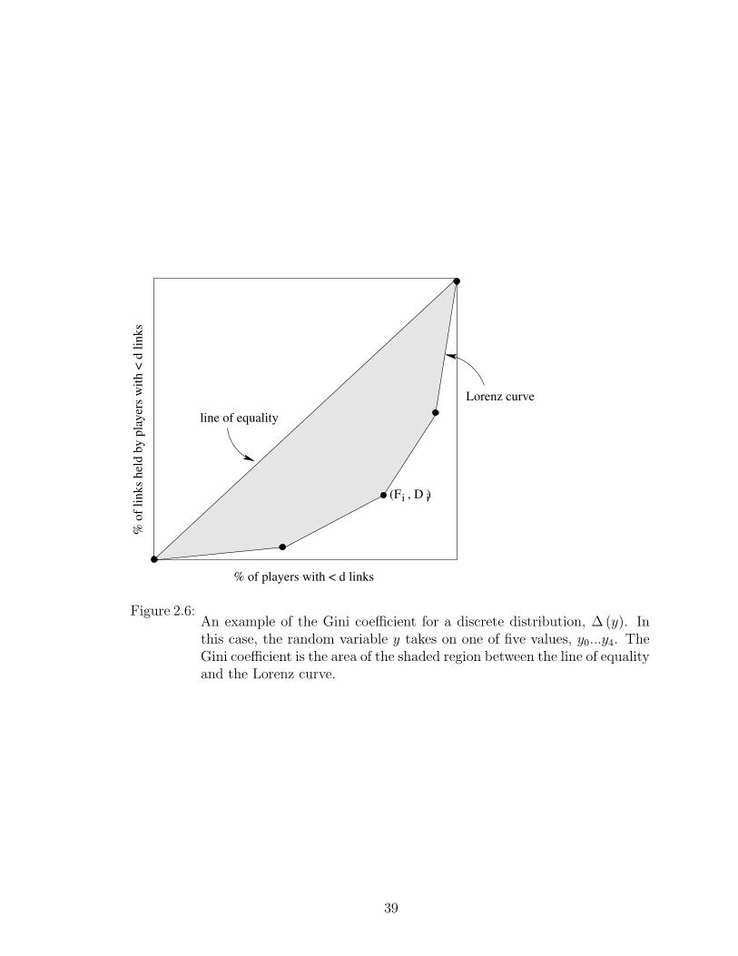
ii(F , D )

% o

f li

nk

s h

eld

by

pla

yer

s w

ith

< d

lin

ks

% of players with < d links

line of equality

Lorenz curve

Figure 2.6:An example of the Gini coefficient for a discrete distribution, ∆ (y). Inthis case, the random variable y takes on one of five values, y0...y4. TheGini coefficient is the area of the shaded region between the line of equalityand the Lorenz curve.

39

the gini coefficient of the degree distribution ∆M,p is

G = 1−(1− pM

)(1− p)

pM[(1− p+ p2)

[(1−p+p2p2

)M− 1

]−M (1− p)

]

It can be shown that δGδM

> 0, meaning that the degree distribution becomes more un-

even as the number of skills required for the problem increases (holding the probability

of having a skill constant).

Figure 2.7 illustrates this comparative static graphically.

M=1

M=4

M=7

M=10

Figure 2.7:A graph of the Gini coefficient, G (p,M), for different populations. Thefour curves pictured represent different values of M , and the x axis rep-resents the value of p. The difficulty of a problem rises as the numberof skills required increases or the probability of having a particular skillfalls.

Together, the two parameters of the Bernoulli skills model reflect the difficulty

of the problem the population faces–a problem is difficult if it requires many skills,

or if the average individual has only a few of them. Theorem 9 can therefore be

interpreted as a comparative static on problem difficulty–the model predicts that as

40

problems become increasingly difficult, a few “superstars” emerge, who participate in

most of the collaborations and help solve a disproportionate number of problems.

2.5 Skill Ladders: Specialization and Degree

In the previous section, I considered a special case in which skills are entirely

uncorrelated. Although there are cases where problem-solving skills are essentially

uncorrelated, we would also like to understand the impact of correlations between

skills. In this section, I consider a case where skills are divided into disciplines, and

the skills within a discipline build on one another, much as calculus builds on algebra

and algebra builds on arithmetic. I show that when skills are correlated in this

way, the degree distribution of the collaboration network becomes even more unequal

than when skills are uncorrelated. This suggests that as fields become increasingly

specialized, a very small number of players will tend to dominate the collaboration

network.

2.5.1 Notation and Definitions

Some additional notation is needed to formalize this concept of specialization. I

will define a ladder to be an ordered set of skills, L = a1, a2, a3...al ⊆ S, such that

any player who has the ith skill in the set must have all of the skills that precede it

in the set.33

Definition 10. A ladder is an ordered set of skills, L = a1, a2, a3...al ⊆ S, such

that Prob (have ai|have ai+1) = 1. An example of a single ladder with 6 skills is

shown in Figure 2.8.

33Page (2007) introduces this concept of skill ladders, where each skill builds on the one before it.

41

a1 a3a2 a5a4 a6

Figure 2.8:A ladder of 6 skills–a player with skill ai in this set must have all of the

skills that precede it: a1...ai−1.

Here, I consider a special case where the skills in S are partitioned into m ladders

of equal length.34 The set of all ladders is denoted S = L1...Lm. Figure 2.9 shows

an example with 12 skills arranged into four ladders.

L3L2L1 L4

Figure 2.9: An example of 12 skills arranged into four ladders of equal length.

I will call a player who has all of the skills in a single ladder an “expert” in that

ladder, and I will call the set of ladders that player i is an expert in Ai ⊆ S.

Definition 11. A player is an expert in a ladder Lk if she possesses all of the skills

in that ladder.34Obviously, since the length of a ladder is an integer, there will only be equal-length ladders if m

divides M evenly. To simplify the exposition, I have written the following as if this is true. However,all of the the following results hold if the ladders are equal length up to integer constraints, whichallows for cases where m does not divide M evenly.

42

One additional assumption will allow us to compare the results in this section to

the results of the Bernoulli skills model. Assume that the conditional probability of

having the next skill in a ladder is the same for all skills–that is, Prob (have ai| have ai−1) =

p for all ai.35 The probability of being an expert in a ladder of l skills is then pl.

The number of ladders, m, will be our measure of how specialized the problem-

solving skills are. Thanks to the above assumption, the case where m = M corre-

sponds to the Bernoulli skills model. On the other extreme, m = 1, and all of the

skills are arranged in a single ladder. Before considering ladders of arbitrary length,

I will first look at this case, where m = 1.

2.5.2 Example: a single ladder of skills

Suppose the skills in the set S comprise a single ladder of length M . Because

Prob (have ai|have ai+1) = 1 ∀i ∈ S, a player’s skill set can be represented by the

number of skills she has (|Ai| = k implies Ai = a1, a2...ak) .

The linking behavior in this case is very simple. The only players who have skill

aM are those who also have skills a1...aM−1. All of the players who don’t have all M

skills link to one of the players who does. The resulting collaboration network is a

set of isolated stars, each with 1−pM

pM links, on average.

Figure 2.10 compares the network structure in the case with one skill ladder

(m = 1) to the network structure in the Bernoulli skills model, where skills are in-

dependent (m = M). The two networks have the same number of skills and players,

and players have the same probability of having an additional skill. This means that

the probability of having all of the skills required to solve the problem is the same in

both networks. Moreover, in both, exactly one player has all of the skills required.

35In other words, I assume that putting a skill at the end of a ladder doesn’t change the essentialdifficulty of obtaining that skill. We could imagine cases where putting a skill at the top of a ladderwould make the skill easier to obtain (eg: because it builds on previous experience). We could alsoimagine a case where skills at the top of the ladder are more difficult to obtain (eg: because they aremore demanding than the skills that came before). These would both make interesting extensions.

43

Figure 2.10:Two collaboration networks with 27 players. In both cases, the playersare solving a problem requiring M = 3 skills. These networks representthe two ends of a spectrum of skill specialization, with m = M ladderson the left and m = 1 ladders on the right.

However, the two networks have a much different structure.

2.5.3 Results for m ladders

Using insights gained from this example, I can derive a more general result. Sup-

pose the skills are arranged in m equal-length ladders.36 As in the previous example,

the only players with all of the skills in a ladder are those who are experts in that field.

Thus, a model with m ladders reduces to a Bernoulli skills model with m independent

skills. Theorem 12 presents a closed-form expression for a player’s degree in the case

with m skill ladders.

Theorem 12. If Ψ is a distribution of skills such that S = L1...Lm is a partition

of S into m equal-length ladders with Prob(

have aji | have aj(i−1)

)= p, then a player

with the skill set A will have expected degree Ed(A) = pM

[(1−p

Mm +p2

Mm

p2Mm

)k− 1

],

36Again, the results are the same if the ladders are equal length to integer constraints.

44

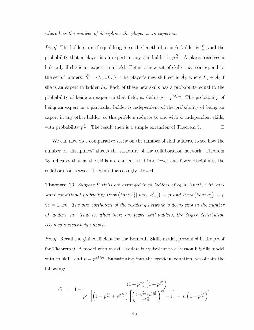
where k is the number of disciplines the player is an expert in.

Proof. The ladders are of equal length, so the length of a single ladder is Mm

, and the

probability that a player is an expert in any one ladder is pMm . A player receives a

link only if she is an expert in a field. Define a new set of skills that correspond to

the set of ladders: S = L1...Lm. The player’s new skill set is Ai, where Lk ∈ Ai if

she is an expert in ladder Lk. Each of these new skills has a probability equal to the

probability of being an expert in that field, so define p = pM/m. The probability of

being an expert in a particular ladder is independent of the probability of being an

expert in any other ladder, so this problem reduces to one with m independent skills,

with probability pMm . The result then is a simple extension of Theorem 5.

We can now do a comparative static on the number of skill ladders, to see how the

number of “disciplines” affects the structure of the collaboration network. Theorem

13 indicates that as the skills are concentrated into fewer and fewer disciplines, the

collaboration network becomes increasingly skewed.

Theorem 13. Suppose S skills are arranged in m ladders of equal length, with con-

stant conditional probability Prob(have aji | have aji−1

)= p and Prob

(have aj1

)= p

∀j = 1...m. The gini coefficient of the resulting network is decreasing in the number

of ladders, m. That is, when there are fewer skill ladders, the degree distribution

becomes increasingly uneven.

Proof. Recall the gini coefficient for the Bernoulli Skills model, presented in the proof

for Theorem 9. A model with m skill ladders is equivalent to a Bernoulli Skills model

with m skills and p = pM/m. Substituting into the previous equation, we obtain the

following:

G = 1−(1− pm)

(1− pM

m

)pm[(

1− pMm + p2 M

m

)[(1−p

Mm +p2

Mm

p2Mm

)m− 1

]−m

(1− pM

m

)]

45

0.1 0.2 0.3 0.4 0.5p

0.985

0.990

0.995

1.000

gini coefficient

Figure 2.11:The gini coefficient for M = 10, divided into different sets of ladders.The bottom curve pictures the case where m = 10, the second curvepictures the case where m = 5, the third shows m = 2, and the fourthshows m = 1.

which is decreasing in the number of ladders, m. Figure 2.11 shows how the gini

coefficient depends on the number of ladders for the case where M = 10.

Skills often build on one another because fields are specialized. The result in

Theorem 13 can thus be interpreted in terms of specialization and reliance on experts–

as skills become increasingly specialized, we would predict that the degree distribution

would become increasingly unequal. This is because when skills are specialized, most

players are not useful collaborators. As a result, most problems are solved by a few,

high-degree experts. On the other hand, when skills are distributed independently,

most players are capable of being useful to someone, and thus the networks will tend

to have a much more even distribution of links.

46

2.6 A Comparison to a Model with a Single Skill

One of the major contributions of the model presented above is its detailed treat-

ment of problem-solving skills. Rather than having a single specialty or“type”, players

in this model have sets of skills, which may overlap. These two models allow for dif-

ferent levels of analysis. In a “type-based” model, a player’s skills are represented by

a single unit–her type. In contrast, a “skill-based” model represents a player’s skills

individually, allowing players’ skill sets to overlap and interact in complex ways. In

this section, I examine how this more general representation of skills impacts network

topology by directly comparing a type-based model of problem-solving to a skill-based

model.

In the previous sections, I showed that when players have sets of skills, the rela-

tionship between a player’s skills and her value as a problem solver is often highly

non-linear. In particular, an individual’s combination of skills may be valuable, even

if her skills are not valuable individually. Since this nonlinearity of degree is driven

by the desirability of combinations of skills, we would expect to regain the linear

relationship between skills and degree in the special case where players’ skill sets do

not overlap–that is, where they have a type or specialty.

Consider the following pair of examples. First, suppose a problem requires 3 skills,

S = a, b, c, and all three skills are distributed independently to each player–that is,

Prob (have skill i |have skill j) = Prob (have skill i)∀i 6= j ∈ S. This means that the

probability of having skill set A is Ψ (A) =∏

i∈A pi. Let pa = Prob (have skill a) = 12,

pb = Prob (have skill b) = 13, and pc = Prob (have skill c) = 1

6. A player in this

population will have, on average, exactly one skill. Table 2.4 shows the expected

degree for all 8 possible combinations of skills. Note that we cannot price individual

skills in such a way that it characterizes a player’s degree in the network. To see this,

suppose that such a pricing scheme existed–that is, suppose ∃µ = [µa, µb, µc] such

that∑

i∈A µi = Ed (A). Then clearly µ (i) = Ed (i) for i ∈ S. But that price scheme

47

A Ψ (A) E [d (A)]

∅ 1036

0a 10

36118

b 536

16

c 236

56

ab 536

59

ac 236

259

bc 136

6abc 1

3618 1

18

Table 2.4:In this example, the problem requires 3 skills: S = a, b, c. The skills aredistributed independently with Prob (have a) = 1

2, Prob (have b) = 1

3, and

Prob (have c) = 16. This table shows the frequency of each skill set, and

the expected degree of an individual with those skills.

would predict that Ed (b, c) = 1, whereas the actual degree of a player with those

skills is Ed (b, c) = 6.

Now, consider a modification of this example–suppose that instead of skills be-

ing distributed independently, we assume that each player has exactly one skill, with

Ψ (a) = 12, Ψ (b) = 1

3,Ψ (c) = 1

6. The population in this example shares many char-

acteristics with the previous population–the frequency of each skill in the population

remains the same, and in both cases, the average player holds one skill. However, in

contrast with the previous example, skills in this population can be priced individu-

ally. If a player has skill i, her expected degree in the cost minimizing collaboration

network is 1−Ψ(i)Ψ(i)

. If we set the prices of skills a, b, and c to be µa = 1, µb = 2, and

µc = 5, then each player’s degree is a linear function of her endowments, weighted by

the prices.

The structure of the collaboration network is also considerably different when

players’ skill sets can overlap. For example, consider the two networks and associated

degree distributions pictured in Figure 2.12. In both cases, the players are solving a

problem requiring three skills: S = a, b, c. In the network on the left, each player

has exactly one skill, and all three skills occur with equal probability (Ψ (a) = Ψ (b) =

48

All players have one skill(type−based)

Players may have many skills(skill−based)

frequency

1

0

.6

.8

.4

.2

2 4

frequency

1

21 43 5 60

.6

.8

.4

.2

6 8 10 12 14 16 18 20

expected degreeexpected degree

Figure 2.12:Contrasting the structure of collaboration networks resulting from type-based and skill-based models of collaboration. In both cases, the problemfaced requires three skills. In the network on the left, each player has asingle skill. In the network on the right, the three skills are distributedindependently with probability p = 1

3. The bottom panels show both

the distribution of degree in the pictured networks (black dots) and thedistribution of expected degree in the set of cost minimizing networks(grey bars).

49

Ψ (c) = 13). In the network on the right, the skills are distributed independently, as

in the Bernoulli skills model, with Prob (have skill i) = 13

for i = a, b, c. In both of

these networks, the average player has one skill. However, the degree distribution

of the collaboration network is much different in the two cases. Every player in the

left hand network has, on average,1− 1

313

= 2 links, and the distribution of links in a

typical cost-minimizing collaboration network is symmetric around that value. In the

left hand network, the network structure is much different. Because combinations of

skills are valuable, players with more skills help to solve a disproportionate number

of problems. The initial inequalities in the distribution of skills in the population are

magnified, resulting in a network of interconnected stars.

This pair of examples illustrates two points. First, the type-based model is a

special case of the skill-based model–in particular, it is the case where each player has

exactly one skill. Second, it highlights the value of a more detailed treatment of skills

in modeling problem solving. Although in some contexts it is appropriate to assume

that each player has a type or specialty, this assumption is not necessarily benign.

That modeling choice impacts our predictions about the value of certain individuals

in the community, as well as impacting the structure of the collaboration network.

In particular, this comparison highlights the difference between modeling the value

of labor in manufacturing production and modeling the value of labor in problem-

solving. In manufacturing, players can plausibly be given a type or specialty, and

the wages of an individual are a function of their type. As production transitions

away from manufacturing towards problem-solving, it becomes more difficult to clas-

sify workers according to a type or specialty. Thus, the shift from manufacturing

production to problem-solving can be modeled as a shift from a type-based model to

a skill-based model. This comparison is particularly valuable because it allows us to

draw conclusions and make predictions about the labor market as we transition from

manufacturing to knowledge-based industries. The following section explores this in

50

greater detail.

2.7 Implications: Labor Markets and Industrial Organiza-

tion

The results of the previous sections have implications on employment, individual

welfare, and training of workers in knowledge-based industries, as well as the internal

organization of firms within those industries. This section examines some of these

implications in greater detail.

2.7.1 Extending the Model to Employment by Firms

Before going further it is worth taking a detour to look at the applicability of

this model outside of collaboration. Although the results of the previous section were

framed in terms of collaboration between individuals, it is relatively simple to extend

this model to firm/employer labor market interactions. Suppose there are two types

of agents in an economy: firms and problem solvers. Firms face problems, which have

value if solved. Let δ be a probability measure on the skill sets required to solve the

firms’ problems–that is, δ (A) is the probability that a firm faces a problem requiring

the skills A ⊆ S, with∑

A⊆S δ (A) = 1. The firms hire problem-solvers to work on

projects, giving them each a share of the proceeds from solving the problem.37 The

expected number of projects a player contributes to can be calculated much the same

way as before:

E [d (A)] =∑C⊆A

δ (C)

σ (C)

The sole difference between this case and that in the previous sections is that now

the demand for a particular set of skills is decoupled from the supply of those skills.

37I will assume that problem solvers don’t bundle themselves together and offer their servicesjointly for a single share of the problem-solving proceeds. This is consistant with the previousinterpretation of the model.

51

Since the proofs of the results in this chapter do not depend on such a coupling, we

can obtain a supermodularity result analogous to Theorem 2 for this firm-based case

as well. As a result, all of the results from previous sections apply to a case where

individuals work for firms, as well as cases where individuals collaborate.

2.7.2 Returns to Skills and Optimal Training Decisions

Although individuals in this model have static skill sets, we can use it to look

at the returns to skills, and thus optimal training decisions. Using the result from

Theorem 2, Theorem 14 shows that in a static population, returns to acquiring new

skills are non-decreasing.

Theorem 14. If a player’s utility is increasing in her degree in the collaboration

network, then players experience non-decreasing returns to obtaining additional skills,

holding the rest of the population fixed.

Proof. This is a simple application of supermodularity.

Theorem 2 states that d (Ai ∪ Aj) + d (Ai ∩ Aj) ≥ d (Ai) + d (Aj). Rearranging,

this tells us that d (Ai ∪ Aj) − d (Ai) ≥ d (Aj) − d (Ai ∩ Aj). Both sides of this

inequality represent a gain in degree from obtaining the skills in the set Aj\Ai. The

fact that this gain is greater when the player already has Ai indicates that returns

are non-decreasing.

The implication of this result is that every player will obtain the maximum num-

ber of skills possible. Thus, this model predicts that a shift in the economy from

manufacturing to knowledge-based production might be accompanied by increasing

returns to skills, and thus increased skill acquisition.

However, that is not the whole story–individuals also have to choose which skills

to obtain in which order. In a world with many possible skills, and costs to ob-

taining new skills, how will a worker determine the optimal skills to acquire? I can

52

calculate the contribution of each skill in a player’s skill set to the total demand

for her skills using a Shapely value decomposition. The demand for player i’s skills

can generically be written as d (Ai) =∑

C⊆Ai

δ(C)σ(C)

where δ (C) = Ψ (S\C)38 and

σ (C) =∑

D⊆S\C Ψ (C ∪D). Using this demand as a value function,39 we can obtain

an expression for the Shapely value of a skill, a, to a player, i.

Theorem 15. The Shapley value for a skill, a, to a player, i, is

φa,i (d) =∑

B⊆Ai\a

1(|Ai||B|

) (∑C⊆B

Ψ (S\ (C ∪ a))∑D⊆S\(C∪a) Ψ ((C ∪ a) ∪D)

)

Theorem 15 shows that the Shapley value of a skill to an individual depends on 1)

the existing skill distribution in the population and 2) the set skills the individual

already has. This theorem suggests that optimal training decisions should be highly

individualized, because the value of a skill depends on problem solver’s existing skill

set and the skills of others in the population.

2.7.3 Variation in Labor Demand

The number of collaborators an individual has (her degree in the collaboration

network) can be interpreted as the demand for her skills as a collaborator. Empirically,

it has been observed that output is highly concentrated among a small number of

people, creating an extremely skewed distribution of demand. For example, Rosen

(1981) observes that in certain creative fields (eg: music, film, textbook writing),

38Note that this is the expression when each player needs exactly one partner to solve theirproblem. The results are similar for the more general case.

39Note that d (.) satisfies both requirements for a value function: d (∅) = 0 and according toTheorem 2, d (A ∪B) + d (A ∩B) ≥ d (A) + d (B), which implies superadditivity.

53

a large fraction of demand goes to an extremely small number of producers. Uzi

and Spiro (2005) observe a similar patter among the directors, producers, and other

creative artists on Broadway. Similarly, data on academic collaborations suggests

that a small fraction of researchers are responsible for the majority of output (see

Newman (2001), Moody (2004), Acedo et al (2006), and Goyal et al (2006)).

This long-tailed distribution has implications for the distribution of wages and

welfare (see the next section for further discussion) and thus there has been consid-

erable interest in understanding why such a concentration in labor demand occurs.

Some existing models (for example, Rosen (1981)) can induce a long-tailed distribu-

tion when there is a high premium on quality, and production technology decouples

effort from output quantity (eg: in creative industries, where a single performance

or album can be enjoyed by many consumers). However, such technologies are not

relevant in knowledge-based industries, where effort is not decoupled from output

volume.

The model presented in this chapter induces a long-tailed distribution of demand

in cases where collaboration is important. As noted above, the search for complemen-

tarities and the bundling of skills within individuals exaggerates existing inequalities

in skill distributions, creating a long-tailed distribution of demand. Thus, this model

can explain uneven output demand when effort is not fixed, but skills are varied.

Moreover, the model makes predictions about the comparative statics of the distri-

bution of output. Specifically, the distribution of demand will become more skewed

as problems become more difficult. We can observe this trend in longitudinal studies

of coauthorship, such as Moody (2004) and Grossman and Ion (2002). These studies

observe the number of collaborations maintained by authors in the fields of sociology

and mathematics, respectively. It is widely believed that the problems faced in these

fields have become more difficult over time. The authors show that the upper tail of

the collaboration distribution extends over time, indicating that a small number of in-

54

dividuals capture an ever-increasing fraction of the collaborative demand. This model

connects those two trends, attributing the attenuation of the demand distribution to

the increasing difficulty of the problems being faced.

2.7.4 Industrial Organization

The results that precede also have implications of the organization of knowledge-

based firms. Traditional organizational structures were hierarchical, with several lay-

ers of supervisors. The theoretical underpinnings of these hierarchical structures are

explored in a wide range of models, including Rosen (1982). However, evidence in-

dicates that organizational structure within firms is changing–hierarchical structures

are flattening, and workplaces are becoming more decentralized (see, for example,

Bresnahan et al (2002) and Rajan and Wulf (2006)).

The model presented in this chapter provides a more general model of organi-

zational structure, one that allows for these more complex interrelationships be-

tween individuals. In particular, this model allows me to explore how a shift to-

wards knowledge-based industries and team-based production affects organizational

structures. In knowledge-based firms, value is created through the creation of new

knowledge, rather than the exploitation of existing knowledge.

My model produces strictly hierarchical structures in one special case–that in

which skills are arranged in a single ladder (see section 2.5.2 for the details of this

case). This case corresponds to a model in which ability is measured on a one-

dimensional scale. One dimensional measures of ability make sense in industries that

create value by exploiting an existing bank of knowledge. However, as demand for

workers shifts towards industries that create value by creating new knowledge, we

expect skills to be arranged in ladders less often. My model predicts that as such

a shift occurs, organizational structure should move away from hierarchies, towards

flatter, more distributed structures.

55

2.8 Extensions

The model I present in this chapter suggests a wealth of extensions. In the fol-

lowing, I will briefly discuss a few of the more promising of these extensions.

2.8.1 Bargaining Over Surplus

As mentioned earlier, there are several reasons to consider an even split of payoffs

between collaborators–indeed, when payoffs to problem solving are non-monetary, it

may be difficult to split returns any other way.40 The results in this chapter also hold

for a variety of other payoff-splitting methods–in particular, the results hold for any

payoff split which induces an individual to minimize the number of collaborators she

has.41

However, one might also want to consider what happens when individuals can

bargain over the surplus from solving a problem. This bargaining process gives each

player a “wage” from the collaboration,42 which I can then use to produce an income

distribution, much as we produce an output distribution in this chapter.

By producing an income distribution, I can attempt to explain some empirical

trends in labor markets. In particular, income inequality has grown dramatically over

the past 50 years, a trend that holds even if one controls for years of education and

tenure (Juhn et al (1991)). The labor literature draws a connection between this trend

towards greater wage inequality and the shift towards knowledge-based production in

our economy, telling a story that is potentially consistent with the model presented

in this chapter: knowledge-based production creates increasing returns to skills, a

trend which benefits high-skilled workers over low-skilled workers, widening the wage

40It is, for example, difficult to split the authorship of a publication into arbitrarily-sized shares.41Note that this is the case whenever an individual’s payoff to solving her problem is decreasing

in the number of collaborators she has. So, for example, if links are costly, the results will be thesame.

42It is possible to show two necessary conditions for non-zero wages: first, firms must face somefriction in hiring (such as search costs) and second, problem solvers must face constraints on theirtime.

56

gap.43 More recent work notes a second-order effect of the shift–the wage distribution

widens most significantly in the upper tail of the distribution. According to Machin

(2008), the wage difference between the 90th percentile and the 50th percentile rose

throughout the 80s, 90s, and early 2000s. On the other hand, the wage difference

between the 50th percentile and wages in the 10th percentile increased significantly

in the 80s, only slightly in the 90s, and actually contracted in the 2000s.

These empirical observations are not inconsistent with the predictions of this

model. As noted in Section 2.6, we can model the shift in production as a shift from

a type-based model to a skill-based model. As production becomes more problem-

solving based, the upper tail of the output distribution stretches dramatically, while

the lower tail contracts, increasing income inequality overall. By explicitly connecting

income to the output, I will be able to determine whether these results on the output

distribution can be extended to the income distribution.

2.8.2 Long Run Skill Acquisition

Thus far, I have assumed that the skill distribution in the population is fixed.

However, in the long run, we would expect problem-solvers to acquire new skills,

based on what will optimize their expected outcomes. I have already shown that in

a static world, the individual’s skill acquisition decisions will depend on the current

state of the world (distribution of skills in the population) and the set of skills the

individual possesses. It would be interesting to look at the long-run steady state

population of problem solvers that results from this dynamic skill acquisition process.

One might ask a number of question about this steady state population. Is the

equilibrium distribution of skills in the population efficient? Do individual players

43See, for example, Juhn et al (1991), who find a trend towards increased wage inequality, andattribute that gap to increasing returns to skills (which they specifically differentiate from yearsof education or tenure). Other, related papers include Kruger (1993) and Berman et al (1998).More recently, Machin (2008) refines this notion, pointing out that technological advances in the 80seliminated many routine tasks, accelerating the increasing returns to skills.

57

acquire too many skills, from a societal perspective? I can also use this model to

ask questions about the equilibrium levels of specialization and generalization in the

problem solving population. Under what conditions should we see individuals spe-

cializing in a set of related skills? In a companion paper, I explore whether specialists

and generalists can coexist in the same equilibrium population. It would also be in-

teresting to see whether, in the extreme long run, disciplines (groups of individuals

with related, specialized skills) emerge. Finally, if the distribution of problems faced

changes over time, then the steady state population may be subject to shocks in the

types of problems faced. A long run model with skill acquisition can explore questions

about the robustness of the populations to these shocks.

2.9 Conclusion

In this chapter, I present a model of problem-solving and collaboration. I use this

model to look at the demand for a problem-solver’s skills as a collaborator. I show

that because a problem solver’s skills are bundled, the number of problem she solves

is a supermodular function of her set of skills–in other words, an individual’s value

as a problem solver is more than the sum of her individual skills. Each additional

skill multiplies the number of skill combinations that the player can use, unlocking

many potential synergies with other problem solvers. Moreover, a player who has a

particularly useful combination of skills may participate in more collaborations than

a player who has many rare skills, but does not fill such a hole in the organization.

The fact that players collaborate with those who have complementary skills also has

an effect on the structure of the collaboration network as a whole–the model predicts

that the degree distribution of a collaboration network will be skewed, even if skills

are distributed independently across players. In other words, the model predicts that

a few players will solve the majority of the problems a population faces, even if the

distribution of skills in the population is symmetrical. Finally, this model connects

58

the nature of problems and problem solvers to the structure of the collaboration

network–as problems become more difficult for a population, the model predicts that

the collaboration network become more centralized around a few, high degree hubs.

In sum, this framework, in which problem solvers have skill sets and collaborate to

solve problems, appears to be sufficiently flexible to address many questions about

the returns to skills in knowledge production.

59

CHAPTER III

Foxes and Hedgehogs: Equilibrium Skill

Acquisition Decisions in Problem-solving

Populations

3.1 Introduction

In this chapter, I consider the decision to be a generalist or a specialist. Being

a generalist is costly. Each of us has a limited capacity for learning new things. By

focusing on a narrow field of study, specialists are able to concentrate their efforts and

maximize the use of that limited capacity. Generalists, on the other hand, are forced

to spread themselves more thinly in the pursuit of a wider range of knowledge. They

pay a penalty for each new field of study they pursue, in the form of effort expended

learning new jargon, establishing new social contacts in a field, and becoming famil-

iar with new literatures. This tradeoff between focus and depth has been observed

empirically in Adamic et al (2010).

In the economics and sociology literatures, it has become common to refer to this

distinction between specialists and generalists via a metaphor, used by Isaiah Berlin

in an essay on Leo Tolstoy: “The fox knows many things, but the hedgehog knows

one big thing” (Berlin (1953)).1 In other words, generalists are foxes, who know

1See, in particular, Tetlock (2005), which uses the metaphor to examine whether specialists or

60

many things, and specialists are hedgehogs, who know one big thing. The question I

will address in this chapter is as follows: given the significant penalty paid by foxes

in acquiring their skills, is there ever a reason that a rational actor would choose to

become one? And is the decision made by individual problem solvers socially optimal?

As I will show in this chapter, it can be difficult to justify the decision to become

a fox. In fact, when problems are simple and disciplinary boundaries fluid, I will show

that it is impossible to rationalize being a fox–obtaining skills in multiple disciplines

is costly, and there are no benefits to doing so. In order to justify becoming a fox,

there must be some advantage to having skills in multiple areas.

Here, I look at two conditions under which foxes can have an advantage over

hedgehogs. First, by virtue of having background in multiple areas, foxes may be

exposed to more ideas and have opportunities to address a wider variety of questions.

Second, if problems have multiple parts, then it may be the case that some elements

of a given problem are best addressed using skills in one discipline and other elements

are best addressed using skills in another discipline. In other words, as problems

become more difficult,2 there may exist problems that are truly interdisciplinary, and

can best be addressed by individuals with skills in many different areas.

The rest of this chapter is as follows. In the first section, I model an individual

problem-solver’s skill acquisition decision–in particular, her decision whether to spe-

cialize in one discipline, or generalize over multiple disciplines. Foxes (generalists)

pay a fixed cost for obtaining skills in a new discipline. In the following two sections,

I use this model to characterize the conditions under which there is a population of

foxes in equilibrium. I show that when problems are simple (consist of only one part),

and there are no barriers to communication between fields, foxes receive no benefit

from diversifying their skills, and in equilibrium all problem solvers will choose to be

generalists make better predictions.2I use the term “difficult” in a similar sense to Page (2008)–difficult problems have many possible

solutions, none of which is optimal, a priori.

61

hedgehogs. When problems are simple, a population of foxes can only be sustained

if there are significant communication or institutional barriers between disciplines,

which prevent specialists in one field from working on problems in another field. In

the presence of such barriers, being a fox is rationalizable as long as problems are

distributed relatively evenly across the different disciplines. I then show that from

a societal perspective, this equilibrium population may be suboptimal. In particu-

lar, there are parameter regions where society would prefer to have some foxes, but

the equilibrium population consists of only hedgehogs. In other words, because foxes

internalize the costs of diversifying their skills, some populations suffer from an un-

dersupply of foxes. This suggests that more problems may be solved by subsidizing

the costs of skill diversification. Finally, I present an extension of the model, which

looks at problems with multiple parts. I show that when problems have more than

one part, a population of foxes can be sustained, even in the absence of institutional

barriers between disciplines.

3.2 Model

I construct a two period model. In period 1, players choose their skills. In period

2, they, as individuals, attempt to solve a problem using those skills. Note that in this

model, there is no collaboration. The problem in period 2 is drawn from a distribution

of problems. Although players know the distribution of problems when making their

skill acquisition decisions, they do not know the particular problem they will face.

Each individual chooses her skills in period 1 to maximize her individual probability

of solving the problem in period 2. I will solve for the equilibrium choice of skills.

Let S be the set of all possible skills.3 The skills are arranged into 2 disciplines,

d1 and d2, each with K skills, s1d...sKd. An example with six skills arranged into

3Skills are defined as bits of knowledge, tools, and techniques useful for solving problems and noteasily acquired in the short run. See Anderson (2010) for a model with a similar treatment of skills.

62

Discipline 1

(d1)

s11

s31

s21Discipline 2

(d2)

s12

s32

s22

Figure 3.1: Two disciplines, each with three skills.

two disciplines is shown in Figure 3.1. A specialist is a person who chooses skills

within a single discipline. A generalist is a person who chooses some skills from both

disciplines.

A problem, y, is a task faced by the individuals in the model. A skill is a piece

of knowledge that can be applied to the problem in an attempt to solve it. Each

skill skd ∈ S has either a high probability (H) or a low probability (L) of solving the

problem. I will define a problem by the matrix of probabilities that each skill will

solve the problem. That is, y =

y11 y12

......

yK1 yK2

where ykd = H if skill k in discipline

d has a high probability of solving the problem and L if it has a low probability of

solving the problem. So, for example, if there are two disciplines, each with three

skills, a problem might be

y =

L H

H H

H L

meaning that two of the skills in each discipline have a high probability of solving the

problem, and one skill in each discipline has a low probability of solving the problem.

63

Define h ≡ 1−H and l ≡ 1− L.

The mechanics of the model are as follows. In period 1, the players, i1...iN , each

choose a set of skills Ai ⊂ S. In period 2, the players attempt to solve a problem

using those skills. I will assume that players have a capacity for learning skills, which

limits the number of skills they can obtain. For the moment, I will assume that all

players have the same capacity for learning new skills. Let M ∈ Z+ represent the

players’ capacities for new skills. For the moment, I will assume that all skills are

equally costly to obtain, and in particular, if qdk is the cost of obtaining skill k in

discipline d, then qdk = q = 1. I will also assume that player pay a fixed cost, c, for

learning skills in a new discipline. That is, players pay 1 + c to obtain the first skill

in a discipline, and q = 1 for every additional skill in that discipline. For simplicity, I

will assume that M = K + c. This assumption means that a specialist can obtain all

K skills in one discipline, and a generalist can obtain a total of K − c skills spread

over the two disciplines.

Although players in period 1 do not know the particular problem they will face,

they do know the distribution from which those problems are drawn. In particular,

they know the probability that each skill will be an H skill or an L skill. I will assume

that the probability that skill skd is an H skill is independent of the probability that

skill sk′d′ is an H skill.4 For the moment, I will also assume that skills are symmetric

within disciplines. That is, I will assume that every skill in a discipline has an equal

probability of being an H skill. This assumption simplifies one decision made by the

players–namely which skills a generalist will choose within each discipline. When skills

are symmetric within a discipline, a generalist’s skill acquisition decision is simply a

division of her skills across the two disciplines–within a discipline, she can choose her

skills at random.

Let δd be the probability that a skill in discipline d is an H skill–that is, δd =

4This assumption means that skills must work more or less independently. That is, it cannot bethe case that skills are used in combination to solve problems, or that skills build on one another.

64

E [Prob (ykd = H)] where the expectation is taken over the distribution of problems,

which I will call ∆. I will assume that the vector of probabilities in the two disciplines,

δ = [δ1, δ2], is known ex ante. This means that while the players do not know the

particular problem they will face, they do know the distribution of problems.

Players choose their skills to maximize their expected probability of solving the

problem in period 2. A Nash equilibrium of this game is a choice of skill set for each

player in the population, A = A1...AN , such that no player has an incentive to

unilaterally change her skill set, given the distribution of problems.

3.3 Results: Specialization and Barriers Between Disciplines

In this section, I consider two questions. The first question concerns individ-

ual decision-making–what is the equilibrium skill acquisition decision of the problem

solvers? Under what conditions do individuals decide to generalize? The second ques-

tion concerns the optimality of that population from a societal perspective. Is the

equilibrium population optimal?

3.3.1 A Special Case: Symmetry Across Disciplines

Before considering the general model, I first look at a special case where δ1 = δ2 =

δ. In this case, all disciplines are expected to be equally useful in expectation. This

case is useful because it produces particularly clear results. The following subsection

generalizes the results from this section to a case where δ1 6= δ2.

Given that generalists pay a significant penalty for diversifying their skills, it is

difficult to explain the existence of generalists in the population. Theorem 16 states

that if there are no barriers to problem solvers working on problems in other fields,

then there will be no generalists in equilibrium.

Theorem 16. If skills are symmetric, and players can work on any available problem,

65

then no player will ever want to be a generalist. In other words, the equilibrium

population will contain only specialists.

Proof. The ex ante probability that a specialist in discipline i will be able to solve a

problem from a given distribution, ∆, is

E [P (Si)] =∑y

Prob (one of skills solves y) ∗∆ (y)

=∑y

(1− Prob (none do)) ∗∆ (y)

= 1−K∑

ni=0

hnilK−ni

(K

ni

)δni (1− δ)K−ni

= 1− (δh+ (1− δ) l)K

where ni is the number of H skills in discipline i in a particular problem, y.

Now, consider a generalist who is spreading his skills across both disciplines. The

ex ante probability that a generalist with x skills in discipline 1 and K − c− x skills

in discipline 2 will solve a problem from a given distribution, ∆, is

E [P (G)] = 1−∑y

Prob (none of skills solve y) ∗∆ (y)

= 1− (δh+ (1− δ) l)K−c

Clearly, 1 − (δh+ (1− δ) l)K > 1 − (δh+ (1− δ) l)K−c, and thus no individual

will ever be a generalist in two disciplines.5

Theorem 16 clearly indicates that when there are no barriers to solving problems

in other fields, there is no advantage to being a generalist. However, in practice,

there may be several barriers between disciplines that prevent individuals in one

discipline from solving problems in another. An individual in one field may simply

5Note that this result generalizes to a case with more than two disciplines. Generalists do worseas they add skills in additional disciplines, so this result holds regardless of the number of disciplinesa generalist spreads himself across.

66

be unaware of problems that exist in other areas, even if her skills would be useful in

solving them. Cultural or institutional barriers may prevent her from working on the

questions she knows about, either because resources are not forthcoming, or because

publication is difficult. Communication barriers are also a significant impediment

to interdisciplinary work–although a physicist may have skills that would be useful

in solving a biology problem, field-specific jargon may make it difficult for her to

communicate her insights, and if communication barriers are severe enough, she may

even have difficulty understanding what open questions exist.

Barriers to working on problems outside ones discipline give specialists a disad-

vantage, because they are only able to work on problems in their own fields. Theorem

32 states that if there are barriers to working on problems outside of ones field, then

a population of all generalists may be sustained in equilibrium. In particular, if there

are two disciplines, and a fraction φ of all problems occur in discipline 1 , then gen-

eralists dominate the equilibrium population for values of φ in a particular range.

As shorthand, let π (δ, h, l) ≡ (δh+ (1− δ) l) be the expected probability that a skill

won’t be able to solve a problem drawn from ∆. Figure 3.2 shows the ranges of φ

in which individuals will specialize and generalize, as a function of π. If a sufficient

fraction of the problems are assigned to one or the other discipline, then all players

will specialize in that discipline. If problems tend to be evenly distributed across

the two disciplines, then players will tend to be generalists and acquire skills in both

disciplines.

Theorem 17. If skills are symmetric, and problems are assigned to one of two dis-

ciplines, then players will generalize (obtain K − c skills spread across the two disci-

plines) if 1 −(

1−πK−c

1−πK

)≤ φ ≤ 1−πK−c

1−πK where φ is the fraction of problems assigned

to discipline 1. If φ > 1−πK−c

1−πK , then the player will specialize in discipline 1 and if

φ < 1−(

1−πK−c

1−πK

)then the player will specialize in discipline 2.

Proof. In this case, the ex ante probability that a problem is solved by a specialist is

67

All specialists in discipline 2

All specialists in discipline 1

!

0 11-!K-c

1-!K

All generalists

!K-!K-c

1-!K

Figure 3.2:The equilibrium skill acquisition decisions as a function of the fraction ofproblems assigned to discipline 1 in the case where skills are symmetricacross disciplines (that is, where δ1 = δ2 = δ). If enough problems areassigned to one of the disciplines, then all players will specialize in thatdiscipline. If problems are more evenly distributed across disciplines, thanplayers will tend to generalize. The point at which individuals will startto generalize depends on π = δh+ (1− δ) l, the expected probability thata single skill will not solve the problem.

φ(

1− (δh+ (1− δ) l)K)

for a specialist in discipline 1 and (1− φ)(

1− (δh+ (1− δ) l)K)

for a specialist in discipline 2. Since generalists can work on problems in both disci-

plines, their expected probability of solving the problem is 1− (δh+ (1− δ) l)K−c. A

player will generalize if E [P (S1)] < E [P (G)] and E [P (S2)] < E [P (G)]. The result

follows immediately.

3.3.2 Optimality of the Equilibrium

The next question that we can ask is whether the distribution of specialists and

generalists in the population is socially optimal. There is reason to believe that it

would not be. From a societal standpoint, we would like to maximize the probability

that someone in the problem solving population manages to solve the problem. Indi-

viduals pay the price for diversifying their skills, which makes it individually rational

to specialize. However, on a societal level, it is optimal to have problem solvers apply

a wide range of skills to the problems faced. Theorem 18 states that for some values

of φ (the fraction of problems that occur in discipline 1) the equilibrium population

68

Generalists

!

0 1

Specialists (d2) Specialists (d1)

Society Prefers Specialists (d1)

Society Prefers Specialists (d2)

Society Prefers Generalists

Ranges in which generalists are under-provided

Figure 3.3:Regions of social suboptimality. The line shows values of the parameterφ–the fraction of problems assigned to discipline 1. The top part of thefigure shows the parameter regions where individuals decide to specialize.The bottom part of the figure shows where specialization is optimal froma societal perspective. The shaded areas indicate the parameter valueswhere individuals choose to specialize, but society would prefer to haveat least a few generalists.

is suboptimal. In particular, there will be an underprovision of generalists. Figure

3.3 illustrates these regions of social suboptimality. Note that these regions will exist

for any value of π ∈ (0, 1).

Theorem 18. If skills are symmetric and problems are assigned to one of two dis-

ciplines, then there is a range of values for φ (the fraction of problems assigned to

discipline 1) such that generalists are underprovided in the equilibrium population of

problem solvers.

In particular, generalists are underprovided when 1−πK−c

1−πK < φ < 1−πN(K−c)

1−πNK or

1− 1−πN(K−c)

1−πNK < φ < 1− 1−πK−c

1−πK .

Proof. The probability that at least one of the N problem-solvers in the population

solves the problem is 1 − Prob (none of them do). If all of the individuals in the

population are specialists in discipline 1, then with probability φ, each specialist

has a probability 1 − πK of solving the problem and πK of not solving it. With

probability 1 − φ, the problem is assigned to the other discipline, and no specialist

69

solves it. Thus, the probability of someone in a population of discipline 1 specialists

solving the problem is

Prob (one of N solve it) = 1− Prob (none of N solve it)

= 1− [φProb (none solve problem in d1)

+ (1− φ)Prob (none solve problem in d2)]

= 1−[φProb (one fails)N + (1− φ) ∗ 1

]= 1−

[φ(πK)N

+ (1− φ) ∗ 1]

= φ(1− πKN

)On the other hand, if they are all generalists, then the probability of at least one

solving the problem is

Prob (one of N solve it) = 1− Prob (none of N solve it)

= 1−(πK−c

)N= 1− πN(K−c)

Society is better off with a population of generalists when 1−πN(K−c) > φ(1− πKN

),

which is true when φ < 1−πN(K−c)

1−πNK . However, there is a population of general-

ists when φ ≤ 1−πK−c

1−πK . It is always the case that 1−πK−c

1−πK ≤ 1−πN(K−c)

1−πNK . So if

1−πK−c

1−πK < φ < 1−πN(K−c)

1−πNK , then society is better off with a population of generalists,

but has a population of specialists.

We can make a similar argument for specialists in discipline 2. Society is better

off with a population of generalists when 1 − πN(K−c) > (1− φ)(1− πKN

), which

is true when φ > 1 − 1−πN(K−c)

1−πNK . However, there is a population of generalists when

φ > 1 − 1−πK−c

1−πK . It is always the case that 1 − 1−πN(K−c)

1−πNK ≤ 1 − 1−πK−c

1−πK . So if

1 − 1−πN(K−c)

1−πNK < φ < 1 − 1−πK−c

1−πK , then society is better off with a population of

70

generalists, but has a population of specialists.

Note that although in this section I have assumed that disciplines are symmetric–

that is, that they are all equally useful for solving problems, in expectation–the results

easily extend to a more general case, where one discipline is more useful, in expec-

tation, than the other. The equivalent results are stated and proved in Appendix

D.

3.3.3 Discussion

In this section, I have shown that because diversifying ones skills is costly, it can be

difficult to justify the decision to be a generalist. The costs associated with learning a

new field, with its new jargon, literature, and social patterns, must be outweighed by

some kind of benefit–in this case, barriers to addressing problems in other fields. In

the real world, there are many reasons that individuals may have trouble working on

problems outside their home discipline. On a purely practical level, communication

barriers make it difficult to understand the content of questions in unfamiliar fields,

and those lacking familiarity with the field may also be unable to place questions in

context. If it is possible to understand the questions, techniques in another field may

be foreign enough to make communicating results extremely difficult. And culturally,

it may be impossible to be taken seriously without credentials in the field a problem

originates in. By possessing some skills in multiple areas, generalists are able to

overcome these barriers and work on problems in many different fields.

However, the final lesson of this section is that the equilibrium level of general-

ization is not always socially optimal. From a societal standpoint, we would like to

maximize the amount of progress made on problems we face. This means applying

skills to all problems that arise. However, when there are barriers to working on

problems outside of ones own field, there is a danger that not all all skills will be

applied to all problems. Generalists are able to apply skills from one discipline to

71

problems in another discipline. However, since they bear the costs of gaining skills in

a new field individually, it is possible for generalists to be underprovided.

3.4 An Extension: Problems with Multiple Parts

In the previous section, I showed that barriers to addressing problems in other

disciplines can induce problem solvers to diversify their skills. In this section, I con-

sider an extension of the previous model, which highlights a second scenario in which

individuals can be incentivized to acquire skills in multiple disciplines: problems with

multiple parts. As problems become more difficult, they may be broken down into

many different sub-problems. Although in some cases, these subproblems may all be

best addressed within a single discipline, in others, different subproblems will be best

addressed using different skills. In this section, I show that when different parts of a

problem are best addressed using different disciplines, then a population of generalists

can be sustained.

3.4.1 Problems With Multiple Parts

Here, I consider an extension of the previous model. Many of the model elements

are the same as before. Once again, the skills in the set S are divided into two

disciplines, d1 and d2. Players use their skills to address a problem, the nature of

which is not known ex ante. They will choose to be a specialist or generalist in period

1 to maximize their chances of solving the problem in period 2.

But now, suppose each problem consists of two parts, y1 and y2. Each part

of the problem is addressed independently by the skills in each of the disciplines.

Thus, much like the problems in the previous section, we can define the parts of the

problem by a matrix of probabilities that each skill will solve the problem. That is,

72

yi =

yi11 yi12

......

yiK1 yiK2

where yikd = H if skill k in discipline d has a high probability

of solving part i and L if it has a low probability of solving part i.

Again, the probability that a given skill is an H skill is not known ex ante. How-

ever, the players know the expected probability that a skill is an H skill. I will

allow the expected probabilities to vary across parts of the problem–in other words,

it is possible that a discipline will be more useful in solving one of the parts of the

problem than in solving the other part of the problem. Let δid be the probabil-

ity that a skill from discipline d is an H skill for part i of the problem. That is,

δid = E [Prob (yikd = H)]. The matrix δ =

δ11 δ12

δ21 δ22

describes a distribution of

problems, ∆, and is known ex ante.

Suppose, that there are just two possibilities for δid: δ1 and δ0, where δ0 < δ1. Then

we can categorize the possible distributions of problems according to which discipline

is useful for which part of the problem. Roughly, these fall into three categories,

which are outlined in Figure 3.4.

In the first category, both disciplines are equally likely to be useful on both parts of

the problem. When this is the case, the results are similar to those obtained in Section

3.3.1, where skills were symmetric across disciplines. In particular, if individuals can

work on any problem they like, then there will be no generalists in equilibrium.

In the second category of problem distributions, one discipline is more likely to

be useful on at least one of the parts. In this case, the results are similar to those

obtained in Section D, where on average one discipline is more useful in solving the

problems faced than the other discipline. Again, if all problems are accessible to all

individuals, no individual will ever chose to be a generalist.

The third category of problems is most interesting. In this category, one of the

disciplines is useful on one of the parts of the problem and the other discipline is

73

X

X

X

X

X

O

X

Oetc...

Category 1: Symmetric across disciplines

X

X

O

O

X

X

X

O

X

X

O

Xetc...

Category 2: One discipline more useful in both parts

X

O

O

X

O

X

X

O

Category 3: Each discipline useful for a different part

Figure 3.4:A taxonomy of problem distributions. In the above, each problem has two

parts. The matrix

[δ11 δ21

δ12 δ22

]represents the distribution of problems,

where δid is the probability of a skill in discipline d being anH skill for parti of the problem. In this case, I have simplified the problem distributionsby assuming that either δid = X (high probability that the discipline willbe useful on part i) or δid = O (low probability that the discipline willbe useful on part i). The problem distributions can be divided into threecategories according to which disciplines are more useful on which partsof the problem.

74

useful on the other part of the problem. This case does not resemble any of those

already explored, and it is the one I will focus on here. This case, where problems

have multiple parts, each of which is best addressed within the context of a different

discipline, presents a different kind of opportunity for generalists than before. Here,

generalists benefit by having diverse skills, useful in different contexts. Note that

unlike in the case where problems are simple (have only one part), when problems

are difficult, there need be no communication barriers in order for individuals to

generalize their skills. Difficult problems can be inherently interdisciplinary, giving

generalists the advantage they need without barriers to working in other fields.

Claim 19. When problems have multiple parts, each of which is best addressed using

a different discipline (eg: δ =

δ1 δ0

δ0 δ1

with δ1 > δ0) then there is a set of values

of π1 = δ1h + (1− δ1) l and π0 = δ0h + (1− δ0) l such that it is individually optimal

for problem solvers to be generalists, even when problems are open.

In order to see this, consider the case mentioned above, where δ =

δ1 δ0

δ0 δ1

with δ1 > δ0. This means that a specialist in discipline 1 will have K skills, all in

discipline 1. Each of her skills has a probability δ1 of being an H skill for part 1 of the

problem, and a probability δ0 < δ1 of being an H skill for part 2 of the problem. In

contrast, a specialist in discipline 2 will have K skills, each of which has a probability

δ0 of being an H skill for part 1 of the problem and a probability δ1 of being an H

skill for part 2 of the problem. A generalist will have skills in both disciplines. When

solving part 1 of the problem, her skills in discipline 1 will have a higher probability

of being H skills. When solving part 2, her skills in discipline 2 will have a higher

probability of being H skills. In this particular case, it will be optimal for a generalist

to split her skills evenly between the two disciplines, and she will obtain K−c2

skills in

each.

For a specialist in either discipline, the expected probability that her skills will

75

0.0 0.2 0.4 0.6 0.8 1.0

0.0

0.2

0.4

0.6

0.8

1.0

!1

!0

Specialists

Generalists

!1 = !0

Equilibrium Skill Acquisition as a Function of !1 and !0

(Two Part Problem with K=3, c=1)

Figure 3.5:Equilibrium decisions to specialize and generalize when problems have twoparts. The boundry between the regions where individuals specialize and

generalize is defined by the equation πK1 +πK0 = (π1π0)K−c

2 − (π1π0)K−c +(π1π0)K . This graph illustrates these regions in the case where K = 3and c = 1. This boundry moves upwards as costs (c) rise, relative to aproblem solver’s capacity (M = K + c).

solve both parts of the problem is E [P (success on part 1)]∗E [P (success on part 2)],

which is(1− πK1

)(1− π0)K where π1 = δ1h+ (1− δ1) l and π0 = δ0h+ (1− δ0) l.

For a generalist, the expected probability that she will solve both parts of the

problem is(

1− πK−c

21 π

K−c2

)2

.

In order to find the parameter region where individuals choose to generalize, we

look for the region where(

1− πK−c

21 π

K−c2

0

)2

>(1− πK1

)(1− π0)K .6 This region, as

a function of π1 and π0, is illustrated in Figure 3.5 for K = 3 and c = 1. As would be

expected, the region where individuals specialize shrinks as the costs to generalizing

(c) become smaller, relative to the individual’s total capacity for learning new skills

(M = K + c).

6Note that when δ1 = δ0, we have a case that fits into the first category in the taxonomy ofproblem distributions in Figure 3.4. Since δ1 = δ0 =⇒ π1 = π0, we can use this calculation toverify the claim made above that in the case where skills are symmetric, the results are the same asin Section 3.3.1.

76

3.5 Conclusion

Given the cost of obtaining skills in new areas, it may seem difficult to rationalize

the decision to diversify ones skills. However, there are clearly a large (and growing)

number of individuals in research communities who choose to do so. In addition,

national funding organizations have put considerable effort into promoting interdis-

ciplinary effort. This chapter indicates that both of those actions can be rationalized

under particular conditions. In particular, it is possible to rationalize the decision

to obtain skills in multiple disciplines if there are significant barriers to working on

questions in fields with which one is unfamiliar. Those who pay the initial price of

learning the jargon and literature of a new field reap the benefits in the form of a

larger pool of problems to solve. These benefits may be even larger if problems are

solved in a collaborative context, making adding collaboration an interesting possi-

ble extension to the current work. In particular, in a collaborative context, people

with skills in multiple disciplines may be able to link specialists in one discipline with

specialists in another discipline.

It is also possible to show that being a generalist is optimal if problems are difficult,

because different parts of a difficult problem may be best addressed using skills in

different disciplines. Again, it would be interesting to allow individuals in this model

to collaborate on problems, because in a collaborative context, we might imagine that

the advantage to generalists would be enhanced.

Finally, the results of this chapter indicate that the equilibrium population of prob-

lem solvers need not be socially optimal. In particular, because generalists internalize

the costs of diversifying their skills, it is possible for generalists to be undersupplied

in the population. If this were the case, a more socially optimal outcome could be

obtained by subsidizing the costs to diversifying ones skills, much as national funding

organizations are now doing. However, it is unclear whether our current situation is

one in which such funding is required. More careful consideration of this question is

77

a good candidate for further work.

78

CHAPTER IV

Team Assembly with Network Constraints

4.1 Introduction

In a group formation game, each player can be a member of one and only one group,

and individual payoffs depend, directly or indirectly, on group structure. Many dif-

ficult and pressing economic problems fall into this category, including rent-seeking,

resource management, contract bidding, volunteer organization, problem solving, and

political lobbying. Depending on the application, the collection of individuals may be

called a group, club, or coalition. However, apart from this basic semantic difference,

all of these problems share the same basic characteristics–they all create incentives,

such as economies of scale, risk-sharing, skill aggregation, and social capital accumu-

lation, that make working within a group (coalition or club) more attractive than

working alone.

Consider, for example, a simple rent-seeking game, in which players compete for

a single rent. There are many incentives for individuals to pool their efforts and

compete as a group: risk averse individuals may be willing to trade some rent in

expectation for a more consistent income stream; a complicated rent seeking task may

require a range of skills; and economies of scale may make larger groups more likely to

win. However, individuals must weigh these advantages against the disadvantages of

higher maintenance costs, free-rider problems, and the division of rents. Many of these

79

incentives come down to a decision over different size groups. Thus, we might think

of this example as one in which individuals have determined that a rent-seeking group

of size 10 maximizes their expected utilities by mitigating risk and taking advantage

of economies of scale. Beyond that ideal size, the losses from managing a larger size

group, free-riding off of others efforts, and division of rents between a larger number

of people reduce the expected utility of the individuals in those groups. However,

they still prefer that larger group to pursuing the rents alone. When a group has

more than 17 members, the costs of maintaining that group make pursuing rents

alone more attractive than staying in the group.

In this chapter, I combine two recent areas of interest–dynamic coalition formation

games and social network constraints–to explore how groups form when individuals

move dynamically and face social, spatial, and institutional constraints on group

membership.

Traditionally, group formation has been modeled statically–that is, players make

their group membership decisions simultaneously–see, for instance, Hart and Kurz

(1983), Nitzen (1991), Yi and Shin (1997), Konishi and Weber (1997), and Heintzel-

man et al (2006). These models are advantageous because of their analytical sim-

plicity and clarity. However, as I will show in Section 4.2.1, static group formation

games often have multiple equilibria, suggesting that there are potentially large gains

to clarifying the process by which they form. The presence of multiple equilibria

raises a new, more complicated set of questions. Which of these equilibria can we

realistically expect to reach given a dynamic group formation process? Will the equi-

librium outcome reached be efficient? What characteristics of the problem affect that

outcome? These questions cannot be addressed using a static model, and thus re-

searchers have increasingly turned towards dynamic models of the coalition formation

process. Recent work spans may different subfields, including industrial organization,

political economy, rent-seeking, and local public good provision and includes (among

80

many others) Bloch (1996), Yi (2000), Arnold and Schwalbe (2002), Konishi and

Ray (2003), Macho-Stadler et al (2004), Arnold and Wooders (2005), and Page and

Wooders (2007).

These dynamic group formation models assume that players are unencumbered

by social, spatial, or institutional barriers to group membership. That is, the play-

ers interact freely with all other individuals in the game and can join any of the

groups in the game without regard to the composition of the group. This is a reason-

able assumption in some contexts, such as political parties, unions, and other large

organizations–however, in many other cases, individuals face substantial barriers in

making their group membership decisions. The nature of these barriers will differ

depending on the context of the specific problem being considered. Barriers to group

membership may be social (eg: an individual can only join a group that contains

someone he knows) or spatial (eg: an individual can only join a group with close

neighbors). Some of these barriers are explicit (eg: a requirement that a current

member “vouch” for the applicant) but others are implicit (eg: a social norm against

attending a party composed only of strangers). The barriers may either limit actions

(an individual is unable to join a particular group) or information (an individual does

not know about the group). However, by modeling these constraints explicitly, we

can look beyond the more superficial of these differences and ask a whole new set

of questions. How do characteristics of the underlying constraint affect the eventual

group structure? Are individuals better or worse off when they are constrained more

heavily? How do constraints of different types affect social welfare?

In this chapter, I model the constraints faced by individuals via a network of

connections–a player can only join a group if she is connected to a current member.

This method allows me to use machinery from the burgeoning networks literature,

which explores how social, spatial and institutional networks affect individual behav-

ior. This literature encompasses a wide range of subfields that (as noted in Jackson

81

(2005)) have only recently started to interact. One branch of the literature has devel-

oped tools used to identify communities within existing social networks (see Fortunato

(2010) for a survey of the literature); another branch examines how limiting interac-

tions between individuals can affect strategic behavior (see, for instance, Galeotti et al

(2007) and Charness and Jackson (2006)); and a third branch explores the dynamics

of how social networks form (see Jackson (2005) for a survey of this work).

By combining elements of these two emerging literatures, I demonstrate the im-

portance of both dynamics and network constraints in the group formation process.

As a baseline for comparison, I start with a static game in which individuals are com-

pletely unconstrained in their choice of groups and show that this game has multiple

equilibria. I then allow individuals to move sequentially, and solve explicitly for the

set of Nash Equilibria of this game. I show that the dynamics act as an equilib-

rium refinement. However, the equilibrium reached in the dynamic game is highly

suboptimal–the negative externality imposed by entering individuals drives groups to

be much too large, relative to the social optimum.

I then compare the grouping behavior of the unconstrained individuals to the

behavior of individuals constrained by an exogenous network of connections. The

network limits a player’s action set to those groups containing individuals she is con-

nected to. I show that the network constraint mitigates the tendency for groups to get

too large. The efficiency of the outcome depends on the topological characteristics of

the network constraint–social welfare is higher when the network is sparse and highly

ordered. This result has the surprising implication that informational, institutional,

and geographic barriers to group membership may actually improve social welfare by

restricting groups from becoming too large.

Finally, I consider optimal institutional design and show that the optimal member-

ship rule also depends on network topology–when a network is dense or random, the

exclusive membership rule (which allows a group to reject members who do not im-

82

prove the group’s welfare) is always optimal. However, when the network is sparse or

highly ordered, the exclusive membership rule can lead to highly suboptimal results.

The structure of the chapter is as follows. In Section 4.2, I introduce a static

coalition formation model, in which individuals choose their group membership si-

multaneously. I characterize the set of Nash Equilibria of that game, and show that

only one is optimal. In Section 4.3, I transform the static model by allowing individ-

uals to make their group membership decisions sequentially over time. This defines a

dynamic game similar to that of Arnold and Wooders (2005). I characterize the set of

Nash Equilibria of this game, and show that a single, highly suboptimal equilibrium

survives. In Section 4.4, I introduce the network constraint. I first characterize the set

of Nash Equilibria of the constrained static game. I then move to the dynamic game

and show how network topology affects social welfare. In Section 4.5, I consider opti-

mal institutional design and show that the optimal membership rule depends on the

topology of the network constraint. In Section 4.6, I conclude and discuss extensions

to the model.

4.2 Basic Model Elements and the Static Game

Before considering the behavior of individuals who face a constraint, I will first

consider a game in which individuals are unconstrained. This game is actually a

special case of the constrained game (ie: one in which all individuals are connected)

and thus provides a good baseline for comparison between this game and the existing

unconstrained literature.

Consider a group formation game withN homogeneous individuals, I = 1, 2, ...N.

An individual can be a member of one and only one group–thus, the group structure

at time t is a partition of I, π(t) =G1G2...GJ(t)

, where Gj denotes the set of

individuals in group j. Note that the number of groups is determined endogenously,

and thus J(t) may vary from one period to the next. The set of all such partitions of

83

the players into groups is denoted Π.

Although all of the games defined in this chapter could be played using a gener-

alized payoff function, in the following I will assume that the players have identical

payoff functions that depend only on the size of the player’s own group. Thus, indi-

vidual i′s payoffs are given by f(gj) where i ∈ Gj and gj = |Gj| is the size of group j. I

also assume that f(g) is single-peaked with maximum value g∗. The assumption that

payoffs depend only on own group size obviously does not allow for externalities be-

tween groups. Nor does it allow players to have preferences over group composition.

However,this is an appropriately simple starting point for dynamic analysis–to the

extent that inter-coalition externalities muddy behavior, they are best left to future

extensions.

I will also assume that payoffs are single-peaked in group size. This assumption is

useful because individual and social preferences are aligned–the individuals all want

to be in groups of size g∗,1 and social welfare is highest when this occurs. I will

show that the equilibrium reached is suboptimal, despite this alignment. The as-

sumption that payoffs are single-peaked also covers nearly all cases that we might

encounter–generalizing further would add considerable complication without yielding

much useful insight. However, extensions to more general payoff forms are obviously

important, and are of interest for future studies. Section 4.6 includes a discussion of

these generalizations.

Define g to be the smallest g such that f(g + 1) < f(2). That is, g is the largest

group that will form before an individual forms a new group of size 2. If f(N) > f(2),

then a new group will never form, and for convenience, I will define g = N in these

cases. Figure 4.1 illustrates an example of g with g < N .

Note that since individuals in this game are homogeneous, the exact arrangement

of the players in the groups is not as important as the sizes of the groups. Thus, I will

1The results that follow can be extended to cases where individuals have different ideal groupsizes, but the results are not particularly illuminating.

84

g g+11 2g

f(g)

g*

Figure 4.1: An illustration of g –the smallest g such that f(g + 1) < f(2).

often find it convenient to refer to the vector of group sizes resulting from a particular

partition of the individuals into coalitions, rather than referring to the partition itself.

To that end, define the group size vector of a partition π(t) = G1...GJ by 〈g1...gJ〉.

Note that the mapping from partitions to group size vectors is many-to-one, and thus

the mapping from equilibrium partitions to equilibrium group size vectors will be as

well.

4.2.1 Static Group Formation Game

Ultimately, the process of group formation is a dynamic one–individuals join,

leave, and form new groups over time. However, the assumption that moves are

made simultaneously may be accurate in some instances and since dynamics add a

good deal of analytical complication to the model, it is reasonable to ask whether

making the model dynamic adds to our understanding of the problem. To that end,

I will first examine a static group formation model. I show that when payoffs are

single peaked in group size, there are often multiple Nash equilibria. In Section 4.3,

85

I allow individuals to choose their group membership sequentially, and show that the

dynamics of the game refine the set of equilibria, leaving a single equilibrium group

size vector. This demonstrates that adding model dynamics can yield insights beyond

those gained from static models.

Consider a static group formation game with N players and payoffs, f(g), single-

peaked in group size. Individuals choose their group membership simultaneously.

We can think of the individuals as choosing a “location”, and all of the individ-

uals who jump to the same location are then members of the same group–thus,

an individual’s behavior strategy consists of a choice of coalition: β ∈ 1, 2...N.

The pair (N, f(g)) defines the static coalition formation game. A Nash equilibrium

of this game is a partition of the players into coalitions, such that no individual

wishes to deviate unilaterally.2 Let Ω (N, f(g)) be the set of partitions of the in-

dividuals into coalitions such that no individuals wishes to move unilaterally–that

is, Ω (N, f(g)) = π = G1...Gj ∈ Π| f (|Gj|) ≥ f (|Gk|+ 1) ∀Gj andGk ∈ π. Let

ε (N, f(g)) denote the set of Nash Equilibrium coalition size vectors induced by those

equilibrium partitions.

In the following, I characterize ε (N, f(g)). This characterization reveals several

interesting aspects of group formation with single-peaked utility and also establishes

the need for equilibrium refinement. 20-22 establish several characteristics that an

equilibrium of the static game will have: 1) the coalitions will mostly be larger than

the social optimum (at most one will be smaller) and 2) all of the groups larger

than the optimum will be approximately the same size. Theorem 23 assembles these

conditions into a complete characterization of ε (N, f(g)). Finally, Theorem 24 puts

a lower bound on the number of equilibria in the set ε (N, f(g)), showing that this

static game will often have multiple equilibria.

Lemma 20 states that in equilibrium, most groups will be larger than the social

2This is equivalent to both an equilibrium in the Open Membership Game from Yi and Shin(1997) and the free mobility equilibrium in Konishi et al (1997)

86

optimum–at most one group can be too small.

Lemma 20. Let (N, f(g)) be a static group formation game with f(g) single-peaked.

If players are unconstrained in their choice of group, then there ∃ no equilibrium

〈g1...gJ〉 ∈ ε (N, f(g)) such that gi ≤ gj < g∗, i 6= j. That is, in equilibrium at most

one group will be smaller than the social optimum.

Proof. Towards a contradiction, suppose ∃ 〈g1...gJ〉 ∈ ε (N, f(g)) such that g1 ≤ g2 <

g∗. f(.) is strictly increasing in that range, so f(g1) < f(g2 + 1). But then players in

group 1 have an incentive to move to group 2, so 〈g1...gJ〉 cannot be an equilibrium

Lemma 20 implies that in characterizing ε (N, f(g)), we need consider only two

cases: either all of the groups are larger than the socially optimal size (g1...gk ≥ g),

or exactly one group is small (g1 < g∗and g2...gk ≥ g∗). The following two Lemmas

address the sizes of the groups in these two different cases. Lemma 21 shows that

in any equilibrium where all groups are larger than the social optimum, the groups

must be approximately the same size. Lemma 22 sets a more restrictive condition in

the case where one group is smaller than the social optimum.

Lemma 21. Let (N, f(g)) be a static group formation game with f(g) single-peaked.

If players are unconstrained in their choice of group, then for all 〈g1...gJ〉 ∈ ε (N, f(g)),

|gi − gj| ≤ 1∀gi, gj ≥ g∗. That is, in equilibrium, all groups larger than the social

optimum must be the same size, up to integer constraints.

Proof. Towards a contradiction, suppose ∃ 〈g1...gJ〉 ∈ ε (N, f(g)) such that g1 > g2 ≥

g∗ and g1 − g2 > 1. f(.) is strictly decreasing in this range, so f(g1) < f(g2 + 1) But

then players in group 1 have an incentive to move to group 2, so 〈g1...gJ〉 cannot be

an equilibrium.

Note that this result extends a result in Nitzen (1991) to the case of single-peaked

utility. Arnold and Wooders (2005) prove a similar result for a sequential game. The

87

following lemma extends that result to the case where one group is smaller than the

social optimum. The Nash Equilibrium requires a slightly stronger restriction on the

size of the groups.

Lemma 22. Let (N, f(g)) be a static group formation game with f(g) single-peaked.

If players are unconstrained in their choice of group, then for all 〈g1...gJ〉 ∈ ε (N, f(g))

such that g1 < g∗3, both of the following must be true:

1. f(gj) ≥ f(g1 + 1) ≥ f(g1) ≥ f(gj + 1) ∀ j > 1

2. gj = gk ∀ j, k 6= 1

Proof. Let 〈g1...gJ〉 ∈ ε (N, f(g))such that g1 < g∗.

Part 1: Consider group 1 (the small coalition) and an arbitrary group j, such that

gj ≥ g∗ Note that f(g1) < f(g1 + 1) and f(gj) > f(gj + 1). If f(g1) < f(gj + 1),

then players in group 1 would move to group k. Similarly, if f(gj) < f(g1 + 1), then

players in group k would move to group 1. Together, these three inequalities imply

f(gj) ≥ f(g1 + 1) ≥ f(g1) ≥ f(gj + 1) ∀ j > 1

Part 2: consider two arbitrary groups, j and k, such that gk ≥ gj ≥ g∗. Lemma

21 indicates that gk − gj ≤ 1. Towards a contradiction, suppose gk − gj = 1, so that

gk = gj + 1. By Part 1, f(gj + 1) ≤ f(g1). Since we assumed gk = gj + 1, this

implies that f(gk) ≤ f(g1). But since f(g1) < f(g1 + 1) to the left of the optimum,

f(gk) < f(g1 + 1), meaning that players in coalition j would move to coalition 1.

Thus, it must be that gj = gk exactly.

Theorem 23 combines the insights from Lemmas 20-22 to fully characterize ε (N, f(g)).

Theorem 23. Let (N, f(g)) be a static group formation game with single-peaked

payoff function f(g). If the individuals are unconstrained in their choice of group, the

set of Nash Equilibria of that game, ε (N, f(g)) , is the union of two sets:

3By Lemma 20, this implies gl ≥ g∗∀l 6= k

88

1. 〈g1...gJ〉 |g ≥ gj ≥ g∗ ∀j and |gj − gk| ≤ 1∀j, k

2. 〈g1...gJ〉 |g1 < g∗, gj ≥ g∗ ∀j 6= 1, gj = gk ∀j, k 6= 1,

and f(gk) ≥ f(g1 + 1) ≥ f(g1) ≥ f(gk + 1)

Example IV.1. A Static Group Formation Game with Logistic Utility

The implications of Lemmas 20-22 and Theorem 23 can be illustrated through

a specific example. Consider a static group formation game with 100 players and a

logistic payoff function f(g) = g(20−g). This function is single-peaked with maximum

g∗ = 10 and g = 17. It is illustrated in Figure 4.2.

g

u=f(g)

g=17g*=10 182

f(g)=g(20!g)

Figure 4.2:Individual payoff function for Example IV.1. Note that the players enjoythe highest payoff in a coalition of size 10.

Lemma 20 indicates that in any Nash equilibrium of this game, at most one

coalition will be smaller than the socially optimal group size, g∗ = 10. Lemma 21

indicates that all of the groups larger than the social optimum will be approximately

the same size. Using these two facts, one can show that there are 5 Nash Equilibria of

this static game: 〈10, 10, 10, 10, 10, 10, 10, 10, 10, 10〉, 〈11, 11, 11, 11, 11, 11, 11, 11, 12〉,

89

〈12, 12, 12, 12, 13, 13, 13, 13〉, 〈14, 14, 14, 14, 14, 15, 15〉, and 〈16, 16, 17, 17, 17, 17〉. Note

that 〈20, 20, 20, 20, 20〉 is not an equilibrium, because an individual in a group of size

20 is better off striking out as an individual.

This example illustrates several difficulties with the static game. First of all, the

set of stable coalition configurations is highly sensitive to the particular parameters

used. For example, with N = 100 individuals, the game illustrated above does not

have an equilibrium with a small group. However, if we change the game slightly,

so that there are N = 101 individuals, there will be an “odd-sized” equilibrium:

〈16, 16, 16, 16, 16, 16, 5〉.

Secondly, most games will have multiple stable group size configurations. In fact,

it is possible to put a lower bound on the number of equilibria for a given game.

Theorem 24 does just that.

Theorem 24. Let (N, f(g)) be a static group formation game. Then |ε (N, f(g))| ≥Ng∗− N

g− 1.

Proof. I will set the lower bound by enumerating the equilibria in which all groups

are larger than the social optimum (ie: the first set in Theorem 23). Note that since

all groups are approximately the same size, each equilibrium with all large groups

is entirely characterized by the number of groups. The largest possible group is g

and the smallest possible group is g∗. Thus, there should be one equilibrium for each

integer in the interval[Ng, Ng∗

],4 or N

g∗− N

g− 1.

Since the lower bound in Theorem 24 is usually greater than 1, the static game

will usually have multiple equilibria. However, the static game provides no insight

into which of those equilibria is most likely to occur. Are they all equally likely, or is

there a distribution of equilibria? Does that distribution depend in a predictable way

4This is actually also a lower bound on the number of equilibria with all large groups. Therecould be more, depending on whether g∗ and g divide N evenly, but including that complication onlyadds more equilibria, keeping the lower bound accurate (albeit a bit lower than is strictly necessary).

90

on the observable elements of a particular problem? These questions are particularly

important because some of the equilibria lead to considerably higher social welfare

than others.

The following section shows that a more dynamic model of the group formation

process, in which individuals make their decisions sequentially over time, provides

an equilibrium refinement. As I will show, not all of the equilibria characterized in

Theorem 23 are attainable when players start the game as individuals.5 Surprisingly,

the surviving equilibrium group size vector is the worst possible of the static equilibria.

4.3 Sequential Group Formation Game–The Unconstrained

Case

While a static group formation game (N, f(g)) will typically have more than one

equilibrium, only one is efficient. This obviously begs the question–will individuals

moving sequentially reach the efficient coalition arrangement, or will they reach an

inefficient outcome? Will that outcome be unique or are several outcomes possible?

In this section, I show that allowing the players to move sequentially refines the set

of equilibria from the static game. When the players start the game as individuals,

they will always reach an equilibrium group structure with the same coalition size

vector. Furthermore, it is not the socially optimal one–when individuals make their

group formation decisions dynamically, they end up in groups that are much too large,

despite a clear alignment between individual and social welfare.

4.3.1 Sequential Coalition Formation Game

In the unconstrained sequential group formation game, individuals are able to

join any currently existing group (Gj ∈ π(t)), or alternatively they can strike off as

5Note that this equilibrium configuration is not a ”Garden of Eden” configuration (Epstein andHammond (2002)) because it can be obtained from some initial configurations.

91

an individual, forming a group of size 1. Thus, individual i’s action set at time

t can be denoted by Ai(t) = π(t) ∪ ∅, where ∅ denotes the action of striking out

as an individual. In the following, I will assume that individuals make their group

membership decisions myopically–that is, they decide which group will maximize their

return, given only the current group structure. This defines a behavior strategy that

simply maps the current group partition, π(t), to the individual’s action set as defined

above: β (π(t)) ∈ Ai(t).

This myopic behavior strategy is identical to that used in Arnold and Schwalbe

(2002) and Arnold and Wooders (2005). The myopia assumption is convenient be-

cause it makes the analysis more tractable. However, in the case of sequential coalition

formation games, it is also behaviorally more reasonable than perfect foresight. The

sequential nature of this game induces an explosion in number of possible states, mak-

ing the sequential coalition formation game more like Chess or Go than Tic-tac-toe.

Moreover, as I will mention later, one can show that myopia is not the sole cause of

the observed behavior, making the assumption relatively innocuous.

(N, f(g), φ) defines an unconstrained sequential coalition formation game, where

φ is a particular order of motion for the players.6 An equilibrium of this dynamic

game is a partition of the players into groups, π = G1...GJ such that f (gj) ≥

f (gk + 1) ∀Gj, Gk ∈ π–that is, a group configuration is an equilibrium if no individ-

ual wishes to deviate unilaterally. Let ε (N, f(g), φ) represent the set of equilibrium

coalition size vectors resulting from those partitions.

Note that any Nash Equilibrium of the dynamic game must be a stable group

configuration in the static game, and therefore ε (N, f(g), φ) ⊆ ε (N, f(g)). Theorem

6This game was first introduced by Arnold and Wooders (2005). However, whereas Arnoldand Wooders consider a Nash Club Equilibrium (a group structure which is stable to deviations bycoalitions of individuals within a particular group) and a k-remainder Nash Club Equilibrium (whichis stable to deviations when k individuals are dropped from the system) I use a Nash Equilibrium.See the later text for a discussion of deviations by groups of n individuals. It is worth noting that Iobtain dramatically different results using the Nash Equilibrium than Arnold and Wooders do usingthe Nash Club and k-remainder Equilibria.

92

25 shows that the sequential game has a unique equilibrium up to the symmetry of the

players. Furthermore, Theorem 26 shows that when players start the game as indi-

viduals,7 this equilibrium is always the worst possible stable group configuration from

the standpoint of social welfare, despite the alignment between social and individual

preferences.

Theorem 25. Let (N, f(g), φ) be an unconstrained sequential group formation game

with f(g) single-peaked. Then there is a unique Nash Equilibrium group size vector,

γ (N, f(g)) = 〈g1...gJ〉, which is a function of the number of players and the payoff

function alone.

Theorem 26. Let (N, f(g), φ) be an unconstrained sequential group formation game

with f(g) single-peaked. Let (N, f(g)) be the static coalition formation game with

the same number of players and payoff function. If 〈g1...gJ〉 is the (unique) Nash

Equilbrium of (N, f(g), φ) then 〈g1...gJ〉 = arg minε(N,f(g))

∑i∈I f(gi). That is, the

Nash Equilibrium of the sequential game is the element of ε (N, f(g)) that minimizes

social welfare.

Proof. Let (N, f(g), φ) be an arbitrary sequential group formation game. Let (N, f(g))

be the corresponding static group formation game. The equilibrium of the static game

(N, f(g))that yields the lowest social welfare is the equilibrium with groups of the

largest size–or conversely, the equilibrium with the smallest number of groups. I will

show that regardless of the order of motion, φ, the players always reach a configura-

tion with the minimum number of groups, and thus the lowest possible social welfare

value.8

7Obviously the equilibrium reached will depend on the initial condition. Starting the game withthe individuals acting alone seems very natural, and also mimics the spirit of the static game. Afull characterization of the basins of attraction for the different equilibria of this game is beyond thescope of the current work. However, I will note that the results that follow are unchanged if theindividuals start the game in a grand coalition.

8Note that an“odd-size”equilibrium (one with a single small group) will always have higher social

93

If f(g) is strictly increasing or decreasing, then the result follows trivially. So sup-

pose f(g) is unimodal. f(g) unimodal implies f(1) < f(2). Thus, the first individual

will always want to start a new group. Since f(g + 1) > f(2)∀ g < g, subsequent

individuals will prefer to join the existing group to forming a new group of size 2. In

fact, it is only worthwhile to create a second group of size 2 when the existing group

is size g. If g ≥ N , then a second group never forms–the individuals ultimately form

one large group of size N and the result follows trivially. So suppose g < N .

For the sake of clarity, let r = Nmodg > 0.9 Thus, the equilibrium in ε (N, f(g))

with the lowest social welfare is the equilibrium with N−rg

+ 1 groups. Regardless of

the order of motion, a new group forms only if all existing groups have reached size

g. Thus, the final group forms only once there are N−rg

groups of size g. This implies

that the unique equilibrium of the sequential game will have N−rg

+ 1 groups.

The basic insights of the proof can best be appreciated via a specific example.

Example IV.2. An Unconstrained Sequential Group Formation Game with Logistic

Utility

Note that while a static group formation game, (N, f(g)), often has multiple equi-

librium group size vectors, only one is efficient. Recall from Example IV.1 that while

the game (100, g(20− g)) has 5 Nash equilibria– 〈10, 10, 10, 10, 10, 10, 10, 10, 10, 10〉,

〈11, 11, 11, 11, 11, 11, 11, 11, 12〉, 〈12, 12, 12, 12, 13, 13, 13, 13〉, 〈14, 14, 14, 14, 14, 15, 15〉,

and 〈16, 16, 17, 17, 17, 17〉– only the equilibrium with groups of size 10 is efficient.

Now, consider the sequential group formation game with the same parameters

and an arbitrary order of play: (100, g(20− g), φ). According to Theorem 25, this

sequential game has a unique equilibrium. Moreover, Theorem 26 indicates that

the equilibrium will be the stable group structure with the lowest possible social

welfare than the equilibrium with the smallest possible number of groups. However, it should becomeclear in the following that such an equilibrium could never arise through sequential movement withthe given initial condition. Therefore, I will not address it explicitly here.

9The same result holds for r = 0, but this assumption simplifies the exposition.

94

welfare–in this case, the configuration with coalitions of size 16 and 17. Note that

this equilibrium is inefficient, because all players are better off in groups of size 10.

The following analysis shows how players wind up in this suboptimal group structure.

The players start the game as individuals, so the first player to move faces a

choice between remaining as an individual and forming a group of size 2. The player

is myopic, so she chooses the group of size 2 because it gives her higher utility in the

next period (Figure 4.3). The second player to move faces a similar choice–she must

g

u=f(g)

21

Figure 4.3:The first individual to move joins another individual to form a group ofsize 2.

decide whether to join the existing large group to form a group of 3, or join another

individual to form a second group of 2. The group of 3 gives her higher utility, so she

joins that group (Figure 4.4).

A new group only forms when f(2) ≥ f(g + 1) where g is the size of the existing

large group. The smallest such g is obviously g– in this case, a group of 17 (Figure

4.5). This is true regardless of how many “large” groups (groups with more than one

individual) there are. Thus, the second group forms when there are 83 individuals

and one group of 17, the third group forms when there are 69 individuals and two

95

g

u=f(g)

2 31

X

Figure 4.4:The second individual to move must choose between forming a new groupof size 2 or joining the existing group of 3. He will choose the group of 3,since it gives him higher utility than the group of 2.

groups of size 17, and so on. The last group forms when there are 15 individuals and

five groups of size 17.

This sixth group is the final group that will ever form. Individuals may (and

indeed, will) move between the existing groups, but no new group will ever form.

The individuals will stop moving when all six groups are approximately the same

size–namely, in the configuration with two groups of size 16 and four groups of size

17: 〈16, 16, 17, 17, 17, 17〉. As predicted by Theorem 26, this is the stable group

arrangement with the lowest possible social welfare value. Note also that at no

point did we specify the order of play–thus, the players will reach the arrangement

〈16, 16, 17, 17, 17, 17〉 regardless of their order of motion.

4.3.2 Discussion–Externalities in Coalition Membership

One might be tempted to attribute the behavior detailed in Theorems 25 and 26

to the players’ myopia. However, it is possible to show that even perfectly forward-

96

g

u=f(g)

1 2 g=17 g+1=18X

Figure 4.5:A new group forms when the large group is size g = 17 because theindividual is better off in a new group of size 2.

looking players will form groups that are larger than the socially optimal size.10 Since

even forward-looking agents reach a suboptimal equilibrium, it is clear that myopia

is not all that is at work in this result.

The cause of the observed behavior is the externality that joining a group imposes

on existing group members. When the group is smaller than the social optimum, that

externality is positive. However, when the group is at the optimal size, the externality

is a negative one. The entering member is obviously made better off by the change

(otherwise, he would not move), but the rest of the group is made worse off. The

negative externality causes individuals to enter a group that does not benefit from

the extra member, which then drives groups to become too large.

Obviously, in the real world, groups of individuals will sometimes make their

membership decisions together. If we allow a subgroup of up to n individuals to move

as a group, then any equilibrium that exists will necessarily have smaller groups.

However, the set of equilibria that are stable to such coalitional deviations are largely

10An example with six players is available from the author upon request.

97

empty (see Arnold and Wooders (2005) for a discussion of this problem). More

importantly, when we move on to games with a network constraint, as in the following

section, it becomes less clear what is meant by a configuration that is stable to

“coalitional deviations”. Analysis of more complicated, network-specific equilibrium

concepts are obviously venues for future work.

Additionally, there is empirical evidence that groups tend to be too large. Many

institutions exist that constrain the size of coalitions, a measure that would be un-

necessary if individuals found themselves in groups of ideal size. In the following

section, I consider the effects of social and spatial constraints on individual behavior

and show that such constraints can improve total social welfare. Section 4.5 con-

tinues this discussion by exploring the effect of the network constraint on optimal

institutional design.

4.4 Sequential Group Formation with a Network Constraint

The analysis of the previous section (as well as much of the existing literature)

assumes that individuals are free to join any existing group, regardless of its current

composition. However, the cases where individuals are completely unconstrained

are relatively few–in most instances, individuals face social, spatial, and information

constraints when making their membership decisions. Consider, for example, a set of

farmers forming water management groups along the banks of a river. Although it

is conceivable that the farmers would organize into groups at random, they are more

likely to join farmers who are adjacent to them on the river than those in a distant

location. Similarly, research groups are more likely to be composed of colleagues than

strangers, and an individual is unlikely to attend a party unless he already knows

someone who is attending.

The most natural way of modeling these constraints is via a network of con-

nections. I give each individual an exogenous network of connections to other peo-

98

ple. An individual can only join a group if it contains a person she is connected

to on the network. More formally, (N, f(g), φ, C) defines a particular sequential

group formation game with a network constraint, where C is an exogenous, un-

changing11 matrix of connections between individuals–that is, Cij = 1 if i is con-

nected to j on the network and 0 otherwise.12 In the constrained game, an indi-

vidual’s action set is restricted to include only those groups she is connected to:

Ai(t) = G |Cij = 1 for some j ∈ G∪∅ ⊆ π(t)∪∅. Clearly such a matrix of connec-

tions can model any set of constraints faced by individual agents, making the network

formulation of this problem extremely general.

However, there is an additional advantage of using a network constraint–namely,

it allows us to draw conclusions about general “classes” of constraints that seem sim-

ilar, without getting caught up in the details of a particular case. For instance, we

might want to determine how individuals on a spatial network behave differently than

individuals on a social network, without getting tied up in the details of a particular

network structure. Fortunately, by varying only a few parameters, we can obtain a

natural spectrum of network structures that correspond nicely to the types of net-

works that we would observe in the real world. For my analysis of network topology

I will use a Watts-Strogatz small world network. This particular network has only

two parameters. The first is average degree, d, which enumerates the average number

of connections each individual in the network has. The second is the Watts-Strogatz

parameter, p ∈ (0, 1), which allows us to examine a spectrum of different network

types–when p = 0, the network is regular and approximates a spatial network; when

11One obvious extension is to allow the network structure to evolve over time. This could provideinsights into network formation. Jackson (2005) provides some background and a survey of thenetwork formation literature.

12Note that this differs significantly from the use of networks in Page and Wooders (2007), whichuses a bipartite network to illustrate the partition of individuals into groups–ie: each individual islinked to the group to which it is a member. Thus, this network contains no information about howindividuals are connected. In this chapter, the network links individuals to one another, restrictingan individual’s choice of groups. Although we could use a second, bipartite network to denote thedivision of players into groups, it adds no insights in the current context.

99

p = 1, the individuals are connected at random; for values of p between 0 and 1, the

network has a “small world” structure, which approximates that of a social network.

13 A pair (d, p) describes a family of networks with similar topological characteristics.

Note that when the network is fully connected, every player knows someone in

every group and therefore Ai(t) = π(t) ∪ ∅. Thus, the unconstrained static and

sequential games considered previously are a special case of the constrained game–

namely one where the average degree is at a maximum: d = N −1. I will first use the

static game to illustrate the effects of the network constraints on individual behavior

given a particular network and then I will show how social welfare is affected by the

network constraint.

4.4.1 The Static Game–Network Constraints and Variable Group Size

As in the unconstrained case, I will start by looking at individual behavior when

players make their group membership decisions simultaneously. This section general-

izes the results of Section 4.2.1 to the constrained case.

An equilibrium of the static game with a network constraint is a partition of the

players into groups that is both feasible and individually rational.

Definition 27. A Nash equilibrium of the game (N, f(g), C) is a partition of the

players into groups, G1...GJ, such that ∀i, i ∈ Gj implies:

1. f (gj) ≥ f (gk + 1) ∀Gk ∈ G1...GJ

2. Cij = 1 for some j ∈ Gj

One result of adding a network constraint is that the analogue to Lemma 21 need

not be true. That is, when players are constrained, there may exist stable group

structures in which groups are different sizes.

13Watts and Strogatz (1998)

100

Claim 28. For a given static group formation game (N, f(g), C), there may exist

a Nash equilibrium group structure, G1...GJ, such that |gj − gk| > 1 for some

gj, gk > g∗.

As an illustration of this claim, consider a game with 12 players on a ring, as

pictured in Figure 4.6. Note that the constraint of the ring could represent either

a constraint on actions (the players would move if they could) or information (the

players would move if they knew). It could also equally well represent an explicit

constraint (a legal constraint), an implicit constraint (a social norm), or a functional

constraint (a geographic coincidence). Further suppose g∗ = 2 and g = 6, so that all

7

11

3

4

5

6

8

10

9

12

1 2

Figure 4.6: A game with 12 players arranged on a ring.

individuals want to be in a group of size 2, and will never form a group larger than size

6. Figure 4.7 illustrates a stable coalition structure of the static game (N, f(g), C)

with uneven group sizes.

It is obvious from Figure 4.7 how the ring affects the stability of this configuration.

The individuals in group C would like to join group A, but they are unable to because

they are not connected to that group on the social network. If the network were

fully connected, the individuals in group C would like to move to group A, and the

configuration would not be stable.

101

C

A

BD

Figure 4.7:An example of an equilibrium group configuration on a ring. Note thatthis would not be an equilibrium on the fully-connected network becausethe players in group C would move group A.

This result is significant because while existing models predict that groups will

be the same size in equilibrium, real-world groups are seldom identical in size. This

analysis indicates that if individuals are constrained, group sizes need not be the same.

By exploiting the fact that any two connected individuals form a fully connected

subgraph, we can extend the results in Theorem 23 to the current case. To do so, we

need one final definition: given a network constraint C, I call two groups, Gj and Gk

connected if ∃h ∈ Gj and i ∈ Gk such that Chi = 1.

Theorem 29. Let (N, f(g), C) be a static group formation game with single-peaked

payoff function f(g) and network constraint C. G1...GJ ∈ ε (N, f(g), C) if for all

connected groups, Gj and Gk, either

1. gj, gk ≥ g∗ and |gj − gk| ≤ 1

or

2. gj < g∗ ≤ gk and f(gk) ≥ f(gj + 1) ≥ f(gj) ≥ f(gk + 1)

102

Proof. Simply note that any pair of connected groups contains a pair of connected

agents, who form a fully connected subgraph of the original graph. The result above

follows immediately from Theorem 23.

4.4.2 The Sequential Game–Network Topology and Efficiency

As in the special case of a fully connected network, the set of equilibria of the

dynamic game is a subset of the equilibria of the static game: ε (N, f(g), φ, C) ⊆

ε (N, f(g), C). However, claim 30 indicates that Theorem 25 need not be true–there

will often be multiple equilibrium group size configurations and the set of equilibria

may depends on the order of play.

Claim 30. A sequential coalition formation game (N, f(g), φ, C) need not have a

unique equilibrium. Furthermore, the set of equilibria of this game may depend on

the order of play, φ.

Examples illustrating this claim can be found in Appendix E.

Since the outcome of the constrained group formation game may depend on the

order of play and random moves and there is no strong theoretical foundation for

a particular order of play or set of random choices, I must somehow deal with this

multiplicity of equilibria. One method would be to determine the distribution of

outcomes combinatorially and calculate the expected social welfare exactly. However,

this method would yield results that are overly narrow, applying only to the specific

networks considered. As discussed earlier, I would like to draw conclusions about a

“class” of networks with similar topologies.

To that end, I will rely on the computational version of the combinatorial argue-

ment above. I will average social welfare over a large number of similar games. In

this case, I use a Watts-Strogatz network, which is constructed as follows. Start with

a regular network of degree d–this is a network in which every individual is connected

to her d2

nearest neighbors on each side. Then, rewire each of the links in the regular

103

graph with probability p. A link is rewired by disconnecting one end and reconnecting

it to a different, random node in the network. Thus, the pair (d, p) describes a family

of networks with a similar topology.

As an illustration of the effect of varying these two parameters, consider a coalition

formation game with 12 players. Figure 4.8 depicts four networks with different

degree. In the first panel, every player is connected to every other player–d = 11.

1 23

4

5

6

8 7

9

10

11

121 2

3

4

5

6

8 7

9

10

11

121 2

3

4

5

6

8 7

9

10

11

121 2

3

4

5

6

8 7

9

10

11

12

Figure 4.8:Four different networks connecting 12 players. Degree of the networkdecreases from left to right. The first panel depicts a fully connectednetwork. As edges are removed at random, average degree declines andplayers potentially become more constrained in their choice of groups.

This is called a fully-connected graph, and represents the special case examined in

Sections 4.2.1 and 4.3. The subsequent panels depict the same network with random

links removed. Obviously, as the degree of the network decreases, the individuals

within that network have fewer choices of groups to join (the size of an individual’s

action set is bounded above by the number of neighbors she has). This parameter

potentially has different meaning in different types of networks–in a spatial network,

the average degree specifies how far an individuals can“see”in all directions14, whereas

in a social network, the average degree varies inversely with the “familiarity” required

for membership.15

14For instance, in the case of the farmers on the river, it might indicate how many upstream anddownstream neighbors an individual can interact with.

15Consider, for example, an individual deciding to join a club. Membership in a college activitymay simply require having an acquaintance in the club. This low threshold of familiarity impliesa densely connected network constraint. Membership in a secret society, on the other hand, mayrequire an applicant to have a very strong social tie to a current member. This network constraintwould be much more sparse.

104

1 23

4

5

6

8 7

9

10

11

121 2

3

4

5

6

8 7

9

10

11

121 2

3

4

5

6

8 7

9

10

11

12

Figure 4.9:Three different networks connecting 12 players. In the first panel, theplayers are connected to their two nearest neighbors on each side. Thisis called a regular network, and is often used to represent arrangementsof individuals in space. In the second panel, a small number of the linksin the regular network are rewired at random. The result is called asmall world network, and is a simple model of a social network. In thelast panel, all of the links in the original network are rewired at random.The result is a random network, similar to those depicted in Figure 4.8.Random networks are easily analyzed, but a poor approximation of socialconnections.

As noted earlier, the parameter p allows us to examine networks with different

topologies. When p = 0, none of the links are rewired, and we have a regular net-

work such as that pictured in the first panel of Figure 4.9. These networks have

a high clustering coefficient (average probability that two of a node’s neighbors are

connected) and a high network diameter (largest minimum path length between two

nodes), and are a good model for spatial networks. On the other hand, when p = 1,

all of the links in the network are rewired at random. The result is a completely

random network, pictured in the last panel of Figure 4.9. These networks have a

low clustering coefficient and low diameter. Although easy to work with statistically,

random networks are unfortunately relatively rare empirically. By rewiring a small,

but non-zero fraction of the links, we obtain a small world network, pictured in the

second panel of Figure 4.9. A small world network has a high clustering coefficient

but low diameter, and is a reasonable first-order approximation of a social network.

In the following analysis, I average social welfare over 100 games with random

order of play and networks with the same pair (d, p). Note that with the exception

105

of the regular networks (p = 0), the network structure will differ from one run to

the next, even as the parameters remain the same. This allows me to average over

a number of networks with the same parameters, which gives the results greater

generality. Since I hope to isolate the effects of network topology on outcomes, the

non-network elements of the game remain the same. All results in this section use a

game with 100 players and logistic utility function f(g) = g(20− g).

Figure 4.10 shows that holding the Watts-Strogatz parameter constant, social wel-

fare declines in the degree of the network constraint.16 Since the size of an individual’s

action set is bounded above by her degree on the network, degree provides a rough

measure of how constraining the network is on individual behavior. As the degree of

the network decreases, the individuals are more constrained in their choice of groups,

which mitigates the tendency for groups to get too large. The fact that social welfare

increases as individuals are more constrained is consistent with the hypothesis that

groups are too large because of a negative externality.

Figure 4.11 shows the effects of the Watts-Strogatz parameter on social welfare.17

As the graph moves from regular, to small world, to random, social welfare declines.

One possible reason for this trend is that as the Watts-Strogatz parameter increases,

the clustering coefficient decreases. The clustering coefficient is the probability that

two of a node’s neighbors are connected. As the clustering coefficient decreases, the

probability that an individual knows more than one person in a group decreases,

and the expected size of the action set increases. Thus, as the clustering coefficient

decreases, the network becomes less constraining and average social welfare declines.

16For Figure 4.10, I used a random graph (p = 1). The results are qualitatively similar for othervalues of p.

17For Figure 4.11, I used networks of degree 2, 4, and 6. The results are qualitatively similarfor networks of different degree. Obviously, as degree increases, the drop in social welfare from theregular graph to the random graph becomes less dramatic.

106

4.5 The Effects of Network Topology on Optimal Institu-

tional Design

The most compelling evidence that real-world groups tend to be too large is that

groups have developed institutions to artificially restrict membership–a measure that

I argue would not be required if individuals self-organized optimally. In this section,

I examine how network topology affects the optimal choice of membership rule.

When individuals are homogeneous, there are only two possible membership rules:18

the “open membership rule” (no restriction on group membership) and the “exclusive

membership rule” (groups can reject a member).19 When individuals are uncon-

strained, the exclusive membership rule is always preferable to the open membership

rule. In other words, the coalition members should never allow the group to get larger

than g∗.

One might think that the exclusive membership rule would always be preferable.

However, Figure 4.12 illustrates that when individuals are restricted in their choice

of groups via a social network, the exclusive membership rule can sometimes result

in group configurations with extremely low social welfare values. An even simpler

example uses a ring network. Suppose 20 individuals are arranged on a ring as shown

in Figure 4.13. If g∗ = 3, then the exclusive membership rule may cause individuals

to be “isolated” between groups of the ideal size. Both of these examples highlight

why the exclusive membership rule is less beneficial when individuals are constrained

in their choice of groups. In the unconstrained case, all of the individuals who were

excluded from other groups could band together. When individuals are restricted,

18Because players are homogeneous, all current members will have the same opinion on whetheror not to admit a new member. Therefore, we need only consider two rules: one where the groupand the individual need to agree, and one where the individual can act as a dictator. Charnessand Jackson (2006) examines how the game play of entire groups depends on the voting rule usedto make decisions within groups. In his case, the individuals may have heterogenous opinions onthe strategic decision, and thus he must consider different types of voting rules. Any extension ofthis work to include heterogeneous players would have to make more careful consideration of how agroup decides to admit or reject a member.

19This terminology was introduced in Yi (2000)

107

they no longer have that option, and there is a much greater chance of individuals

being forced into low utility outcomes.

Once again, more general results can be obtained by averaging over many runs

on topologically similar networks. Figure 4.14 shows that when degree is low, the

exclusive membership rule is no longer the clear optimal choice. Similarly, Figure

4.15 shows that when the graph is very ordered, the exclusive membership rule is,

on average, less beneficial. Given the possibility of extremely poor outcomes, such

as those pictured in Figures 4.12 and 4.13, the open membership rule may be more

desirable when the network constraint is low degree or highly ordered.

4.6 Extensions and conclusions

The model I have introduced in this chapter lends itself to numerous interest-

ing extensions. Although I have chosen a very simple payoff function for this ini-

tial work, the basic game structure of the model is easily generalized to model any

problem in which payoffs depend on coalition structure. For instance, by making

payoffs a function of the entire coalition size vector (f (g1g2...gJ)), we can include

inter-coalitional externalities. This would allow us to model (among other things)

a sequential version of the traditional 2-period rent-seeking game (such as that in

Nitzen (1991)) or resource-allocation game (such as that in Heintzelman et al (2006))

and ask whether inter-coalitional externalities are affected by the structure of the

underlying network constraint. For example, we might ask whether social welfare

is higher when resource management groups are formed according to geography (eg:

water management groups on a river) or social/family ties (eg: fisheries on a bay).

If we allow heterogeneity of players, then the payoff function might depend on

the composition of the groups, as well as their size (f (G1G2...GJ)), which would

allow us to explore another set of problems. If individuals are heterogeneous in

ability or tool sets, then we can ask where self-organized teams contain an optimal

108

level of diversity for problem-solving. If individuals are heterogeneous in ideology,

we can explore the formation of lobbyist organizations and political parties. More

abstractly, if individuals are heterogeneous in an arbitrary characteristic, we can

model discriminatory behavior.

Finally, making the network structure endogenous may add some insight into net-

work formation (See Jackson (2005) for an excellent survey of this growing literature).

This might be accomplished either by making links weighted, or allowing links to be

added an lost over time.

The process of group formation is one that has attracted increasing interest in the

past decade. In this chapter, I use a simple extension of a static coalition formation

game to illustrate the importance of dynamics and membership constraints in the

coalition formation process. I show that in the sequential coalition formation game,

individuals tend to form groups that are too large, especially when players are un-

constrained. Real world groups often implement membership restrictions, indicating

that without such restrictions, the groups would tend to be too large. I also show

that if individuals are constrained by a network, they tend to form groups that are

closer to the ideal size, without the addition of membership restrictions. In fact, con-

straining group membership by requiring a social or spatial connection can effectively

substitute for the institutional constraint of a membership rule.

109

Average Efficiency--Random Graphs o(ideal group size = 10)

average degree

average efficiency

2 4 6 8 1012141618202224262830323436384042444648505254565860626466687072747

0.54

0.55

0.56

0.57

0.58

0.59

0.6

0.61

0.62

0.63

0.64

0.65

0.66

0.67

0.68

0.69

0.7

Figure 4.10:Define efficiency to be ratio of actual social welfare to the maximum pos-sible social welfare. This plot shows average efficiency over 100 runs of asequential coalition formation game with N = 100 and f(g) = g(20−g).The network constraints are random (p = 1). As the degree of thenetwork constraint decreases, social welfare increases. Social welfareincreases because the constraint binds more heavily, mitigating the ten-dency for groups to get too large.

110

Average Efficiency--Watts Stro(ideal group size 10)

probability a given link is rewired

average efficiency

0 0.1 0.2 0.3 0.4 0.5 0.6 0.7

0.7

0.75

0.8

0.85

0.9

Figure 4.11:Define efficiency to be ratio of actual social welfare to the maximumpossible social welfare. This plot shows average efficiency for 100 runsof a sequential coalition formation game. For all runs, N = 100 andf(g) = g(20 − g). Holding degree constant (at 2, 4, 6) average socialwelfare declines in the Watts-Strogatz parameter–that is, social welfareis higher when the network is ordered than when it is random.

111

Figure 4.12:An example in which the Exclusive Membership Rule induces a pooroutcome. In this game, g∗ = 3. If groups are able to deny membership,there is a possibility that more central individuals will form one group,leaving the outliers to a poor payoff. This degree distribution of thisnetwork is that of a hierarchical social structure.

Figure 4.13:An example illustrating how the Exclusive Membership Rule can bedetrimental on a ring. This is a game with 20 individuals arranged ona ring and g∗ = 3. Because the large groups can prevent them fromjoining, the isolated individuals must accept a lower payoff.

112

Average Efficiency--Veto (ideal group size 10)

degree

average efficiency

2 4 6 8 1012141618202224262830323436384042444648505254565860626466687072747

0.5

0.55

0.6

0.65

0.7

0.75

0.8

0.85

0.9

0.95

1

Figure 4.14:Comparing the exclusive membership rule to the open membership rulefor network constraints of different degree.

113

Average Efficiency--Watts Stro(ideal group size 10)

probability a given link is rewired

average efficiency

0 0.1 0.2 0.3 0.4 0.5 0.6 0.7

0.7

0.75

0.8

0.85

0.9

Figure 4.15:Comparing the exclusive membership rule to the open membership rulefor network constraints with different Watts-Strogatz parameters.

114

CHAPTER V

Conclusion and Extensions

The research agenda started by the work in this thesis is fairly ambitious. The the-

sis itself is a small step in the direction of understanding the interplay between skills,

problem solving, and collaboration networks and the work contained here suggests

many pathways for future research. In the chapters themselves, I have mentioned a

few of the more modest extensions, some of which represent works in progress. In this

concluding section, I will look at a few of the more ambitious possibilities suggested

by this work.

Empirical connection between skills and degree

In Chapter 2, I make a connection between the set of skills an individual has and

her position on the collaboration network. This connection is valuable, because it has

the potential of providing a clearer explanation of the variation in outcomes among

problem solvers. If one assumes that skills contribute to an individual’s success as

a problem solver in a linear manner, when in fact skills interact with one another,

we will be able to explain a relatively small amount of the variation in outcomes

based on skills. Moreover, the problem becomes worse if we, as researchers, are

unable to observe skills that are known to the agents themselves. If we assume that

skills contribute to outcomes in a linear fashion, then unobserved skills reduce the

115

amount of variation we can explain in a linear fashion. On the other hand, if skills

contribute to outcomes in combination, there will be a nonlinear drop-off in explained

variation with every unobserved skill. Thus, it would be valuable to be able to test

the predictions of this model in a real world collaborative setting.

Unfortunately, data that links skills and collaborative success is relatively rare.

However, with the increase in freely-available online data, there are several new and

exciting data sources that might be used. One particularly good source of data on

skills and problem solving comes from the world of large-scale online gaming. In

large-scale games, such as World of Warcraft, individual players work together in

groups to solve puzzles and complete tasks. The advantage of this data is that it

contains very explicit information about individuals’ skills and the tasks that they

complete. Moreover, because skills are measured within the context of the game,

and easily observed by both other players and the researcher, empirical work is quite

clean. Other possible sources of data include patent and grant-writing networks. In

both of these, there is usually a sense of which individuals bring which skills to the

table. In particular fields, the number of patents or grants written is large enough to

produce a network that is reasonably well-connected. The observability of skills in

this data is less clear than in large-scale gaming, which makes this data more difficult

to work with. On the other hand, the context of that data is closer to the kinds

of problems that are relevant to businesses and universities, making it a worthwhile

avenue to pursue.

Collaboration and skill acquisition

In Chapter 3, I take a first look at some questions surrounding the acquisition

of skills. The results of that chapter are the first step into what is clearly a rich

and valuable field of research. One particularly compelling sets of questions would

consider equilibrium skill acquisition in the context of collaboration. In this thesis, I

116

have mostly considered skill acquisition in the context of individual problem solving.

It would certainly be valuable to consider the equilibrium decisions individuals would

make if they were working in a more collaborative environment. One might suspect

that specialists and generalists would play different roles in a collaborative environ-

ment, and perhaps occupy different positions in the collaboration network. Modeling

these questions theoretically will require a considerable amount of work, but may

provide insights into the “ecology” of collaborative communities.

Empirically, it would be interesting to study the connection between specialization

of skills and outcomes. Data on this subject is becoming increasingly available as

more individuals participate in work-based online social networking. In the context of

academic collaboration, one might ask questions about how an individual researcher’s

outcomes depend on her advisor’s position in the social network. Do individuals

whose advisors are more central to the network do better on the job market, holding

all other factors equal? One could also consider the connection between focus and

outcomes. Suppose we look at the committee members for two young researchers.

In one case, the researcher’s committee members are all located in a single, tight-

knit collaborative community within the collaboration network. In the other case,

the committee members are spread across a wide range of relatively disconnected

collaborative communities. All other things equal, which of these researchers will

have a better outcome? Will the individual whose committee resides in a single

community benefit from having greater focus? Or will the individual with a wide-

spread committee benefit from a greater diversity of ideas and social information?

Finally, we might consider skill-acquisition in a much more long-run context. In

the extreme long-run, we would suspect that the kinds of problems faced by a problem-

solving community (such as a group of academic researchers) would have an effect

on the skills acquired by those individuals. We might expect that over time, skills

would cluster into groups, based on the combinations of skills that are useful for

117

solving different kinds of problems. Thus, we might expect to observe the evolution

of disciplines over time. It would be interesting to look at the robustness of these

equilibrium communities to shocks in the kinds of problems faced. It may be that

communities become “overfitted” to the distributions of problems they face, causing

failures when that distribution experiences external shocks. On the other hand, it

may be that by sustaining a small population of generalists, these communities are

robust to the effects of shocks.

Dynamic, long run model of networks and collaboration

As mentioned in the introduction to this thesis, there are two aspects to the re-

lationship between social network structure and behavior. On the one hand, social

networks clearly affect individual behavior–they shape interactions between individ-

uals and a person’s position in the network affects how others view her. On the other

hand, social network structure is clearly a product of individual behavior. Chapters

2 and 4 of this thesis address these two aspects of network formation individually.

However, there is clearly a feedback between the two. Who a person knows now af-

fects who she is able to interact with in the future, both because she is more likely

to interact with new people through your existing social network, and also because

others’ perceptions of your quality as a collaborator depend on your position in the

network. Linking the effects of network structure on behavior into a more dynamic

model of network formation is a difficult task. However, it promises to provide in-

sights into the evolution of collaborative communities, and the networks that support

them.

118

APPENDICES

119

APPENDIX A

Pairwise Stability and Efficiency

Briefly, a network is pairwise stable if no individual would prefer to terminate an

existing link, and if no pair of individuals would prefer to add a link. Although this

definition is usually used in undirected networks, it works equally well in the current

context. Formally, a collaboration network, g, is pairwise stable if

1. for all ij ∈ g, ui (g) ≥ ui (g − ij) and uj (g) ≥ uj (g − ij)

2. for all ij /∈ g, if uj (g + ij) > uj (g) then ui (g + ij) < ui (g)

Together, these two conditions ensure that links are mutual. That is, if a network is

pairwise stable, then both players agree to maintain the link.

Theorem. Any cost minimizing collaboration network, g ∈ Γ (Ψ), is pairwise stable.

In other words, ∀ij ∈ g ui (g) ≥ ui (g − ij) and uj (g) ≥ uj (g − ij) and for all ij /∈ g,

if uj (g + ij) > uj (g) then ui (g + ij) < ui (g).

Proof. Let g be a cost-minimizing collaboration network. First, consider whether any

player wishes to unilaterally remove a link, ij ∈ g. Severing this link deprives player

j of his share of the payoff from solving i′s problem,(

1|Ci|+1

≥ 0)

, and thus he will

never choose to terminate one of his incoming links. Since player i chooses a minimal

120

set of collaborators that allowed her to solve the problem, removing a link means

that she can no longer solve the problem and no longer receives a payoff. Since her

share of the payoff is greater than zero(

1|Ci|+1

≥ 0)

, this ensures that she will also

never choose to severe a link unilaterally. Finally, note that no player will ever want

to add an outgoing link to a cost-minimizing collaboration network–because every

player has chosen a set of collaborators optimally, any additional link would require

her to further split her prize.

Theorem. Any cost minimizing collaboration network, g ∈ Γ (Ψ), is strongly effi-

cient. In other words,∑

i ui (g) ≥∑

i ui (g′) ∀ g′ ∈ G.

Proof. Because all value is generated from solving problems, the maximum possible

value in the network is N . Since solving the problem is incentive compatible for every

player, and the payoff from solving the problem is split evenly between collaborators,

with no loss, the players always extract the maximum value from the network.

121

APPENDIX B

General Proof of Supermodularity

Theorem. For any distribution of skills, Ψ, a player’s expected degree over the net-

works in Γ (Ψ) is a supermodular function of her set of skills. That is, E [d (A ∪B)]+

E [d (A ∩B)] ≥ E [d (A)] + E [d (B)].

Proof. A player with the set A∪B will be able to help players needing any subset of

those skills. Let δ (C) be the demand for a particular set of skills, C. In the general

case,

δ (C) = Ψ (S\C) +∑

D : Ψ(C∪D)=0

Ψ (S\ (C ∪D))

. The fraction who can supply the set C is σ (C) =∑

D⊆S\C Ψ (C ∪D). Note that

δ (C) and σ (C) depend only on the particulars of the problem (S), the distribution

of skills (Ψ), and the subset of skills (C). Thus, any player with the skill set A ∪ B

has expected degree

E [d (A ∪B)] =∑

C⊆A∪B

δ (C)

σ (C)

We can divide the problems that a player with A∪B can solve into three groups:

1. Requires only skills from set A: C ⊆ A

122

2. Requires only skills from set B, including at least one found only in B:

C |C ⊆ B and∃ b ∈ C st b ∈ B\A

3. Requires at least one skill from each set that can only be found in that set:

C |C ⊆ A ∪B, where∃ a, b ∈ C s.t. a ∈ A\B and b ∈ B\A

Using this partition, we can write

E [d (A ∪B)] =∑C⊆A

δ (C)

σ (C)+

∑C⊆B andC∩B 6=∅

δ (C)

σ (C)+

∑C⊆A∪B andC∩A,C∩B 6=∅

δ (C)

σ (C)

= E [d (A)] +∑

C⊆B andC∩B 6=∅

δ (C)

σ (C)+ φ

which implies that

E [d (A ∪B)] + E [d (A ∩B)] = E [d (A)] +∑

C⊆B andC∩B 6=∅

δ (C)

σ (C)+ φ+ E [d (A ∩B))]

= E [d (A)] +

∑C⊆B andC∩B 6=∅

δ (C)

σ (C)+

∑C⊆A∩B

δ (C)

σ (C)

+ φ

= E [d (A)] + E [d (B)] + φ

≥ E [d (A)] + E [d (B)]

123

APPENDIX C

Shapley Value of Each Skill in a Skill Set

We can calculate the contribution of each skill in a player’s skill set to the total

demand for her skills using a Shapely value decomposition. The demand for player i’s

skills can generically be written as d (Ai) =∑

C⊆Ai

δ(C)σ(C)

where δ (C) = Ψ (S\C)1 and

σ (C) =∑

D⊆S\C Ψ (C ∪D). Using this demand as a value function,2 we can obtain

an expression for the Shapely value of a skill, a, to player i:

φa,i (d) =∑

B⊆Ai\a

1(|Ai||B|

) (∑C⊆B

Ψ (S\ (C ∪ a))∑D⊆S\(C∪a) Ψ ((C ∪ a) ∪D)

)

This decomposition highlights several points that have been made earlier in the paper:

first, the value of a skill to a player depends on the rest of the skills that player has,

and second, the value of a skill depends on the population of problem solvers.

1Note that this is the expression when each player needs exactly one partner to solve theirproblem. The results are similar for the more general case.

2Note that d (.) satisfies both requirements for a value function: d (∅) = 0 and according toTheorem 2, d (A ∪B) + d (A ∩B) ≥ d (A) + d (B), which implies superadditivity.

124

In the particular case of the Bernoulli Skills Model, we can make several other

observations. In this case, the value of skill a to player i is

φa,i (d) = pM (1− p)k−1∑j=0

(1− j

k

)(1− p+ p2

p2

)j

Skills are symmetric in the Bernoulli Skills model, and thus each skill has the same

value to a particular player–that is, φa,i = φi∀a ∈ Ai. Also, because skills are dis-

tributed independently, the value of a skill to a player is strictly increasing in the

number of skills the player already has–that is, φa,i > φa,j iff |Ai| > |Aj|.

125

APPENDIX D

A More General Case: Asymmetric Disciplines

Theorem 31 is the equivalent of Theorem 16, and states that if individuals can

work on any available problem, then there is no advantage to being a generalist.

Theorem 31. If skills are symmetric within disciplines, and players can work on any

available problem, then no player will ever want to be a generalist. In other words,

the equilibrium population will contain only specialists.

Proof. As above, the ex ante probability that a specialist in discipline i will be able

to solve a problem from a given distribution, ∆, is

E [P (Si)] = 1− (δih+ (1− δi) l)K

= 1− πKi

where πi = (δih+ (1− δi) l).

WLOG, suppose δ1 > δ2. Since h < l, this means that π1 < π2 and E [P (S1)] >

E [P (S2)]. Thus, to determine whether any player will generalize, I need to compare

E [P (S1)] to E [P (G)].

The ex ante probability that a generalist with x skills in discipline 1, and K−c−x

126

skills in discipline 2 solves a problem from a given distribution, ∆, is

E [P (G)] = 1− (δ1h+ (1− δ1) l)x (δ2h+ (1− δ2) l)K−c−x

= 1− πx1πK−c−x2

Since π1 < π2, E [P (G)] is strictly increasing in x. This means that a generalist

will set x = K − c − 1 and E [P (G)] = 1 − πK−c−11 π2, which is clearly less than

E [P (S1)] = 1− πK1 .

Theorem 32 is a generalized version of Theorem 17, and states the parameter

range in which individuals will choose to diversify their skills when there are barriers

to working interdisciplinarily.

Theorem 32. If skills are symmetric within disciplines, and problems are assigned

to one of two disciplines, then players will generalize for intermediate values of φ, the

fraction of problems assigned to discipline 1.

In particular, the ranges are as follows:

• If δ1 = δ2 = δ, players will obtain K − c skills spread across the two disciplines

when 1− 1−πK−c

1−πK ≤ φ ≤ 1−πK−c

1−πK , K skills in discipline 1 when φ > 1−πK−c

1−πK , and

K skills in discipline 2 when φ < 1− 1−πK−c

1−πK .

• If δ1 > δ2, then players will obtain K − c− 1 skills in discipline 1 and one skill

in discipline 2 when 1−(

1−πK−c−11 π2

1−πK2

)≤ φ ≤ 1−πK−c−1

1 π2

1−πK1

, K skills in discipline

1 when φ >1−πK−c−1

1 π2

1−πK1

, and K skills in discipline 2 when φ < 1−(

1−πK−c−11 π2

1−πK2

).

• If δ2 > δ1, then players will obtain K − c− 1 skills in discipline 2 and one skill

in discipline 1 when 1−(

1−πK−c−12 π1

1−πK1

)≤ φ ≤ 1−πK−c−1

2 π1

1−πK1

, K skills in discipline

1 when φ >1−πK−c−1

2 π1

1−πK1

, and K skills in discipline 2 when φ < 1−(

1−πK−c−12 π1

1−πK2

).

Proof. In this case, the ex ante probability that a problem is solved by a specialist

is φ(1− πK1

)for a specialist in discipline 1 and (1− φ)

(1− πK2

)for a specialist

127

in discipline 2. Since generalists can work on problems in both disciplines, their

expected probability of solving the problem is 1 − πx1πK−c−x2 where x is the number

of skills the generalist chooses to acquire in discipline 1. First, suppose δ1 > δ2. Since

h < l, this means that π1 < π2 and E [P (G)] is strictly increasing in x. Thus, a

generalist will choose a minimal number of skills in the less useful discipline, and

E [P (G)] = 1− πK−c−11 π2.

A player will generalize if E [P (S1)] < E [P (G)] and E [P (S2)] < E [P (G)]. Set-

ting φ(1− πK1

)< 1−πK−c−1

1 π2 implies that φ ≤ 1−πK−c−11 π2

1−πK1

. Setting (1− φ)(1− πK2

)<

1 − πK−c−11 π2 implies that 1 − 1−πK−c

1−πK ≤ φ. We can verify that in the appropriate

ranges, players choose to specialize. The result follows immediately. The proof for

δ2 > δ1 is similar. For the proof when δ1 = δ2, see Theorem 17.

Finally, Theorem 33 is the generalization of Theorem 18. It states that there is a

parameter region in which individuals choose to specialize, but society would prefer

to have at least a few generalists.

Theorem 33. If skills are symmetric within disciplines and problems are assigned to

one of two disciplines, then there is a range of values for φ (the fraction of problems

assigned to discipline 1) such that generalists are underprovided in the equilibrium

population of problem solvers.

In particular, generalists are underprovided in the following ranges:

• If δ1 = δ2, then generalists are underprovided when 1−πK−c

1−πK < φ < 1−πN(K−c)

1−πNK or

1− 1−πN(K−c)

1−πNK < φ < 1− 1−πK−c

1−πK

• If δ1 > δ2 , then generalists are underprovided when1−πK−c−1

1 π2

1−πK1

< φ <1−πN(K−c−1)

1 π2

1−πNK1

or 1− 1−πN(K−c−1)1 π2

1−πNK2

< φ < 1− 1−πK−c−11 π2

1−πK2

• If δ2 > δ1 , then generalists are underprovided when1−π1π

K−c−12

1−πK1

< φ <1−π1π

N(K−c−1)2

1−πNK1

or 1− 1−π1πN(K−c−1)2

1−πNK2

< φ < 1− 1−π1πK−c−12

1−πK2

128

Proof. First, suppose that δ1 > δ2. The probability that at least one of theN problem-

solvers in the population solves the problem is 1 − Prob (none of them do). If all of

the individuals in the population are specialists in discipline 1, then every individual

has probability φ of a problem occurring in her discipline. In that case, each specialist

in discipline has a probability 1 − πK1 of solving the problem and πK1 of not solving

it. With probability 1 − φ, the problem is assigned to the other discipline, and no

specialist solves it. Thus, the probability of someone in a population of specialists

solving the problem is

Prob (one of N solve it) = 1− Prob (none of N solve it)

= 1− [φProb (none solve problem in d1) + (1− φ)Prob (none solve problem in d2)]

= 1−[φProb (one fails)N + (1− φ) ∗ 1

]= 1−

[φ(πK1)N

+ (1− φ) ∗ 1]

= φ(1− πKN1

)Through a similar argument, if everyone in the population is a specialist in dis-

cipline 2, then the probability that someone in the population solves the problem is

(1− φ)(1− πKN2

).

If everyone in the population is a generalists, then the probability of at least one

person in solving the problem is

Prob (one of N solve it) = 1− Prob (none of N solve it)

= 1−(πK−c−1

1 π2

)N= 1− πN(K−c−1)

1 πN2

Society is better off with a population of generalists than a population of dis-

cipline 1 specialists when 1 − πN(K−c−1)1 πN2 > φ

(1− πKN1

), which is true when

129

φ <1−πN(K−c−1)

1 πN2

1−πNK1

. However, there is a population of generalists when φ ≤ 1−πK−c−11 π2

1−πK1

.

It is always the case that1−πK−c−1

1 π2

1−πK1

≤ 1−πN(K−c−1)1 π2

1−πNK1

. Thus, if1−πK−c−1

1 π2

1−πK1

< φ <

1−πN(K−c−1)1 π2

1−πNK1

, then society is better off with a population of generalists, but has a

population of specialists.

Through a similar argument, society is better off with a population of generalists

than a population of discipline 2 specialists when 1−πN(K−c−1)1 πN2 > (1− φ)

(1− πKN2

),

which is true when φ > 1− 1−πN(K−c−1)1 πN

2

1−πNK2

. However, there is a population of generalists

when φ ≤ 1− 1−πK−c−11 π2

1−πK2

. It is always the case that 1− 1−πN(K−c−1)1 π2

1−πNK2

≤ 1− 1−πK−c−11 π2

1−πK2

.

Thus, if 1− 1−πN(K−c−1)1 π2

1−πNK2

< φ < 1− 1−πK−c−11 π2

1−πK2

, then society is better off with a pop-

ulation of generalists, but has a population of specialists.

The proof for δ2 > δ2 is similar. See the proof of Theorem 18 for the case where

δ1 = δ2.

130

APPENDIX E

Examples Where Sequential Coalition Formation

Game Have No Unique Equilibrium

I will illustrate the second half of this claim first–that the order of play can affect

the set of Nash Equilibria. Consider a game with 12 players arranged in a ring, as

shown in Figure 4.6. Further, suppose the payoff function is f(g) such that g∗ = 2

and g = 6.

For the first case, suppose that the players proceed in order around the ring–

that is, φ1 = (1, 2, 3, 4, 5, 6, 7, 8, 9, 10, 11, 12). Figure E.1 shows game play leading

to an equilibrium coalition structure with two groups of size six. Because of the

order of play, the individuals are always choosing between joining an existing large

group, forming a new group of two, or remaining as an individual. This choice is

much the same as the choice players face in the unconstrained game with the same

payoff function–pictured Figure E.2. Thus, it should be unsurprising that the players

reach the same equilibrium coalition structure as they would in the unconstrained

game: 〈6, 6〉. In fact, this is the only equilibrium coalition size vector possible in this

particular coalition formation game.

Now consider a second game with the same number of players, network constraint,

and payoff function, but a different order of play φ2 = (2, 3, 5, 6, 8, 9, 11, 12, 1, 7, 4, 10).

131

11

10

1 2

3

5

4

6

78

9

12

11

10

1 2

3

5

4

6

78

9

12

11

10

1 2

3

5

4

6

78

9

12

11

10

1 2

3

5

4

6

78

9

12

11

11

10

1 2

3

5

4

6

78

9

12

10

1 2

3

5

4

6

78

9

12

11

10

1 2

3

5

4

6

78

9

12

11

Order of Movement: 1, 2, 3, 4, 5, 6, 7, 8, 9, 10, 11, 12

10

1 2

3

5

4

6

78

9

12

Figure E.1:In this game, 12 individuals are arranged in a ring. The payoff function,f(g), has maximum g∗ = 2 and g = 6. The individuals move in orderaround the ring–φ1 = 1, 2, 3, 4, 5, 6, 7, 8, 9, 10, 11, 12–and wind up in twogroups of size 6. In fact, 〈6, 6〉 is the only equilibrium group size configu-ration of the game (12, f(g), φ1). Figure E.3 shows the same game witha different order of play.

Figure E.3 shows one possible sequence of game play, given φ2. Because the first few

players to move are separated from the existing large groups, they are unable to

impose on the groups that have already formed, as they did in the previous example.

The result is an equilibrium coalition structure with four groups of the ideal size:

〈3, 3, 3, 3〉. Since 〈3, 3, 3, 3〉 is in ε (N, f(g), φ2, C) but not in ε (N, f(g), φ1, C), it is

clear that the order of motion does affect the set of equilibria.

Of course, the outcome pictured in Figure E.3 is not the only possible equilibrium

of the game with order of play φ2. Many players in this game are forced to make

random choices. Figure E.4 shows that if some of those players make different choices,

then the players will find themselves in a different configuration–in this case, 〈4, 4, 4〉.

132

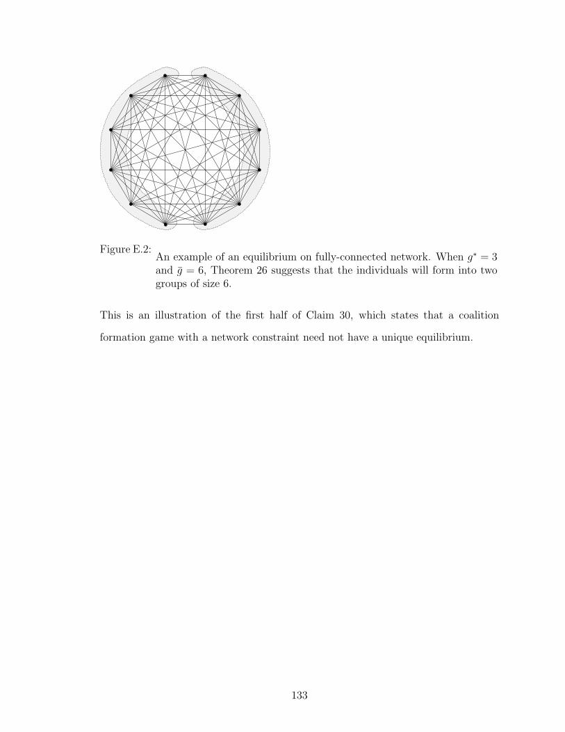
Figure E.2:An example of an equilibrium on fully-connected network. When g∗ = 3and g = 6, Theorem 26 suggests that the individuals will form into twogroups of size 6.

This is an illustration of the first half of Claim 30, which states that a coalition

formation game with a network constraint need not have a unique equilibrium.

133

11

10

1 2

3

5

4

6

78

9

12

10

1 2

3

5

4

6

78

9

12

11

10

1 2

3

5

4

6

78

9

12

11

10

1 2

3

5

4

6

78

9

12

11

10

1 2

3

5

4

6

78

9

12

11

10

1 2

3

5

4

6

78

9

12

11

10

1 2

3

5

4

6

78

9

12

11

10

1 2

3

5

4

6

78

9

12

11

10

1 2

3

5

4

6

78

9

12

11

Figure E.3:This game is identical to the game presented in Figure E.3 except for theorder of motion: φ2 = 2, 3, 5, 6, 8, 9, 11, 12, 1, 7, 4, 10. This figure showsa particular sequence of moves, which leads to groups of the ideal size:〈3, 3, 3, 3〉. Note that 〈3, 3, 3, 3〉 is not an equilibrium of the game pre-sented in Figure E.3, proving that the set of equilibria may depend onthe order of play.

134

10

1 2

3

5

4

6

78

9

12

11

10

1 2

3

5

4

6

78

9

12

11

10

1 2

3

5

4

6

78

9

12

11

10

1 2

3

5

4

6

78

9

12

11

10

1 2

3

5

4

6

78

9

12

11

10

1 2

3

5

4

6

78

9

12

11

11

10

1 2

3

5

4

6

78

9

12

10

1 2

3

5

4

6

78

9

12

11

10

1 2

3

5

4

6

78

9

12

11

10

1 2

3

5

4

6

78

9

12

11

10

1 2

3

5

4

6

78

9

12

11

Figure E.4:This game is identical to that presented in Figure E.3. Note, in particular,that the order of play is the same: φ2 = 2, 3, 5, 6, 8, 9, 11, 12, 1, 7, 4, 10.However, the players have made different random choices, leading to adifferent equilibrium outcome: 〈4, 4, 4〉. This shows that when players aresufficiently constrained, there need not be a unique equilibrium coalitionsize configuration.

135

BIBLIOGRAPHY

136

BIBLIOGRAPHY

Acedo, F. J., C. Barroso, C. C. Rocha, and J. L. Galan (2006), Co-authorship in man-agement and organizational studies: An empirical and network analysis, Journalof Management Studies, 43 (5), 957–983.

Adamic, L. A., X. Wei, J. Yang, S. Gerrish, K. K. Nam, and G. S. Clarkson (2010),Individual focus and knowledge contribution, working Paper.

Arnold, T., and U. Schwalbe (2002), Dynamic coalition formation and the core, Jour-nal of Economic Behavior and Organization, 49, 363–380.

Arnold, T., and M. Wooders (2002), Dynamic club formation with coordination,Warwick Economic Research Papers, 640.

Berman, E., J. Bound, and S. Machin (1998), Implications of skill-biased technologicalchange: International evidence, Quarterly Journal of Economics, 133 (4), 1245–1279.

Bloch, F. (1996), Sequential formation of coalitions in games with externalities andfixed payoff division, Games and Economic Behavior, 14, 90–123.

Bresnahan, T. F., E. Brynjolfsson, and L. M. Hitt (2002), Information technology,workplace organization, and the demand for skilled labor: Firm-level evidence, TheQuarterly Journal of Economics, 117 (1), 339–376.

Burt, R. S. (2001), Structural Holes versus Network Closure as Social Captial, chap. 2,pp. 31–56, Aldine Transaction.

Calvo-Armengol, A. (2004), Job contract networks, Journal of Economic Theory,115 (1), 191–206.

Calvo-Armengol, A., and M. O. Jackson (2004), Social networks in determining em-ployment: Patterns, dynamics, and inequality, American Economic Review, 94 (3),426–454.

Charness, G., and M. O. Jackson (2007), Group play and the role of consent innetwork formation, Journal of Economic Theory., 136 (1), 417–445.

Coleman, J., E. Katz, and H. Menzel (1957), The diffusion of innovation amongphysicians, Sociometry, 20 (4), 253–270.

137

Copic, J., M. O. Jackson, and A. Kirman (2005), Identifying community structuresfrom network data, working Paper.

DeGroot, M. H. (1974), Reaching a consensus, Journal of the American StatisticalAssociation, 69, 118–121.

DeMarzo, P. D., D. Vayanos, and J. Zwiebel (2003), Persuasion bias, social influence,and unidimensional opinions, Quarterly Journal of Economics, 118, 909–968.

Fafchamps, M., M. J. van der Leij, and S. Goyal (2006), Scientific networks andcoauthorship, in The University of Oxford, Department of Economics DiscussionPaper Series, vol. 256.

Galeotti, A., S. Goyal, M. O. Jackson, F. Vega-Redondo, and L. Yariv (2007), Networkgames, European University Institution Department of Economics Working Papers.

Girvan, M., and M. Newman (2002), Community structure in social and biologicalnetworks, Proceedings of the National Academy of Sciences, 99 (12), 7821–7826.

Girvan, M., and M. Newman (2004), Finding and evaluating community structure innetworks, Physics Review E, 69 (2), 69–84.

Gleiser, P. M., and L. Danon (2003), Community structure in jazz, Advances inComplex Systems, 16 (4), 565–573.

Golub, B., and M. Jackson (2007), Naive learning in social networks: Convergence,influence and the wisdom of crowds, working Paper.

Goyal, S., M. J. van der Leij, and J. L. Moraga-Gonzalez (2006), Economics: Anemerging small world, Journal of Political Economy, 144 (2), 403–412.

Granovetter, M. S. (1973), The strength of weak ties, American Journal of Sociology,78, 1360–1380.

Granovetter, M. S. (1995), Getting a Job: A Study of Contacts and Careers, 2 ed.,University of Chicago Press.

Guimera, R., B. Uzzi, J. Spiro, and L. A. N. Amaral (2005), Team assembly mech-anisms determine collaboration network structure and team performance, Science,308, 697=702.

Hagel, J. I., J. S. Brown, and L. Davidson (2009), Measuring the forces of long-termchange: The 2009 shift index, Deloitte Center for the Edge.

Hagerstrand, T. (1967), Innovation Diffusion as a Spatial Process, Chicago: Univer-sity of Chicago Press.

Hart, S., and M. Kurz (1983), Endogenous formation of coalitions, Econometrica,51 (4), 1047–1064.

138

Heintzelman, M. D., S. W. Salant, and S. Schott (2009), Putting free-riding to work:A partnership solution to the common-property problem, Journal of EnvironmentalEconomics and Management, 57, 309–320.

Hong, L., and S. E. Page (2001), Problem solving by heterogeneous agents, Journalof Economic Theory, 97, 123–163.

Hong, L., and S. E. Page (2004), Groups of diverse problem solvers can outperformgroups of high-ability problem solvers, Proceedings of the National Academy ofSciences, 101 (46), 16,385–16,389.

Iyer, B., C.-H. Lee, and N. Venkatraman (2006), Managing in a ’small world ecosys-tem’: Lessons from the software sector, California Management Review, 48 (3),28–47.

Jackson, M. O. (2005), A Survey of Models of Network Formation: Stability andEfficiency, Cambridge University Press.

Jackson, M. O. (2008), Social and Economic Networks, Princeton University Press.

Jackson, M. O., and B. Rogers (2007), Relating network structure to diffusion prop-erties through stochastic dominance, The B.E. Journal of Theoretical Economics,7 (1), 1–13.

Jackson, M. O., and A. Wolinsky (1996), A strategic model of social and economicnetworks, Journal of Economic Theory, 71 (1), 44–74.

Juhn, C., K. M. Murphy, and B. Pierce (1993), Wage inequality and the rise in returnsto skill, Journal of Political Economy, 101 (3), 410–442.

Konishi, H., and D. Ray (2003), Coalition formation as a dynamic process, Journalof Economic Theory, 110, 1–41.

Konishi, H., M. Le Brenton, and S. Weber (1997a), Pure strategy nash equilibrium ina group formation game with positive externalities, Games and Economic Behavior,21, 161–182.

Konishi, H., S. Weber, and M. le Brenton (1997b), Free mobility equilibrium in alocal public goods economy with congestion, Research in Economics, 51, 19–30.

Kruger, A. B. (1993), How computers have changed the wage structure: Evidencefrom microdata 1984-1989, Quarterly Journal of Economics, 108 (1), 33–60.

Lipnack, J., and J. Stamps (1993), The TeamNet Factor: Bringing the Power ofBoundary Crossing Into the Heart of Your Business, John Wiley and Sons.

Machin, S. (2008), Big ideas: Rising wage inequality, CentrePiece, 13 (2), 8–10.

139

Macho-Stadler, I., D. Perez-Castrillo, and N. Porteiro (2006), Sequential gormationof coalitions through bilateral agreements, International Journal of Game Theory,34, 207–228.

Moody, J. (2004), The structure of a social science collaboration network: Disciplinarycohesion from 1963 to 1999, American Sociological Review, 69 (2), 213–238.

Newman, M. (2001), Scientific collaboration networks. i. network construction andfundimental results, Physical Review E, 64, 016,131.

Newman, M. (2003), Properties of highly clustered networks, Physical Reveiw E, 68,026,121.

Newman, M. E. J. (2006), Finding community structure in networks using the eigen-vectors of matrices, Physical Reveiw E, 74, 036,104.

Nitzen, S. (1991), Collective rent dissipation, The Economic Journal, 101 (409), 1522–1534.

Page, F. H., and M. Wooders (2007), Networks and clubs, Journal of EconomicBehavior and Organization, 64, 406–425.

Phillips, K. W., E. A. Mannix, M. A. Neale, and D. H. Gruenfeld (2004), Diversegroups and information sharing: The effects of congruent ties, Journal of Experi-mental Social Psychology, 40, 497–510.

Polzer, J. T., L. P. Milton, and J. William B. Swann (2002), Capitalizing on diversity:Interpersonal congruence in small work groups, Administrative Science Quarterly,47 (2), 296–324.

Powell, W. W., K. W. Koput, and L. Smith-Doerr (1996), Interorganizational col-laboration and the locus of innovation: Networks of learning in biotechnology,Adminitrative Science Quarterly, 41 (1), pp 116-145., 41 (1), 116–145.

Rajan, R. G., and J. Wulf (2006), The flattening firm: Evidence from panel dataon the changing nature of corporate hierarchies, The Review of Economics andStatistics, 88 (4), 759–773.

Rosen, S. (1981), The economics of superstars, The American Economic Review,71 (5), 845–858.

Rosen, S. (1982), Authority, control, and the distribution of earnings, The Bell Jour-nal of Economics, 13 (2), 311–323.

Ryan, B., and N. C. Gross (1943), The diffusion of hybrid seed corn in two iowacommunities, Rural Sociology, 8, 15–24.

Thomas-Hunt, M. C., T. Y. Ogden, and M. A. Neale (2003), Who’s really sharing?effects of social and expert status on knowledge exchange within groups, Manage-ment Science, 49 (4), 464–477.

140

Topa, G. (2000), Social interactions, local spillovers and unemployment, Review ofEconomic Studies, 68 (2), 261–295.

Uzzi, B., and J. Spiro (2005), Collaboration and creativity: The small world problem,American Journal of Sociology, 111 (2), 447–504.

Uzzi, B., L. A. Amaral, and F. Reed-Tsochas (2007), Small-world networks and man-agement science research: a review, European Management Review, 4, 77–91.

Watts, D., and S. Strogatz (1998), Collective dynamics of ’small-world’ networks,Nature, 393, 440–442.

Yi, S.-S. (1997), Stable coalition structures with externalities, Games and EconomicBehavior, 20 (201-237).

Yi, S.-S., and H. Shin (2000), Endogenous formation of research coalitions withspillovers, International Journal of Industrial Organization, 18 (2), 229–256.

141