.f ,

1

\

A STUDY OF RESONANCE MECHANISMS

FOR NONLINEAR ATMOSPHERIC FLOWS

by

Michael Lazare ,.

A thesis submitted to the Faculty of Graduate Studies and Research in partial fulfilment of the requirements for a degree of Master of Science.

Department of Meteorology McGill University Montreal

August. 1979

: )

J 1

1

{-,.

- i i-

(, ,.

ABSTRACT

, The forced~ weakly non-' inear barotropic vortlicity equation wiUr small

initial ampl itude perturbations superimposed on a uniform zona 1 flow is '- {1 ! n

studied ilna1ytically. The basic -types of nonl inear interactions among

Rossby waves are investigated. Wh en resonant forcing is present, nonl inear

effects due to the excitation of waves other, than the stationary mode ("no; se") _ • ct. ~

can ultimately modify the linear response .. In the limit of smafl inHial ,

noise, both mOda~nd resonpnt tr'lad interactions permit large responses,

whereas the response is considerably redueed for larger initial noise.

rt i s argued that Egger' s (1978) resonance meeha~ism ;nvoiv;ng forced­

forced wave interactions is probably not efficient in the presence <;>f initial

noise. In more realist;c baroel;nic shear flows, a resonant growth ;5

possible .in the absence of ,background noise, provided that certain

restrictions on the background floware satisfied. This might help explain

the appea rance bloçking activity.

,

)

,. Il

\

t

/

,

(

-III.

-11,-./'

" ,

RESUME

On ~tudie analytiquement " 'êquation barotrope forc~e du tourbillon

incluant des termes de faible nonlinêaritê. Cette ~quation décrit des

perturbations de faible amplitude initi-ale superposêes a un écoulement '",

zonal uniforme. On examine les prineipau~ types d'interaction nonlinéaire

entre des ondes de Rossby, En prés~nce de fOrçage~rOdUi sant de 1 a

résonance, l es effets nonl inêa ires dOs a " excitation d" ondes autres que

stationnaire ("brui'!: de fond") peuvent êver'ttuellement modifie'r 1-8 rêponse , l

linéaire. Dans la limite 00 le bruit de fond est faible initialement, les ,

interactions modales ainsi que les interactions de triade rêsonnante

permettent de grandes rêponses, tandi s que cell es-ci sont con~idérabTement 4-

-réduites p9ur un brui t de fond important.

On prétend que le mêcanisme de rêsonanee de Egger (1978), lf1!pl iquant

un couple d'ondes forcées interagissantes, n'est probablement pas efficace •

en présenc~ de bruit de fond initial. Dans le casop.lus réaliste d'lm )

écoulement barDel ine, une croissance résonnante est possible en l'absence , -

de bruit de fond., pourvu qu'il satisfasse certaines conditions. Cette idée fT

pourrait contribuer a expliquer la formation de blocage a grande échelle.

."' , .. /

q

,1

l

l "

p

\ '

(.

(

'0

-iv-

fl ,

Il ACKNOWLEDGEMENTS

,

The authortlJuld like to perSona 11 Y thank the thesis supervisor, . J 1"

Dr. T. Warn, for ~ntroducing him to tl1is problem and/for his invaluable

aid in understanding the compléxities involved. His guidance, criticisms

and helpful suggestions, w'hieh 'led to many stimulating discussions, are """,,-, 1

-..... 1<

reflected in a major portion of this work. ,

l am also indebted to the National S!:ience and Engineerin~ Research

Coùncil and to McGill University for their flnancial 'support during .the Ic

research period. Finally, 1 wish to thank Ms. Ursul a Seidenfuss for

drafting the figures and Mrs. D. Mathewson for her typing of the manuscript.

J /

,1

f

/

.1

, .J

p

-,

(

Figure 2.1

SAO

-vi-

LIST OF FIGURES , ! '\ ;_i

Locus of pairs of wavevectors k1 'and k2 whiçh ~orm a resonant

triad with.ko fo'r \1=0.5,4>0=135°, and \Ï<012/n 2 =17 (curve 1),

50 (curve 2), and 97 (curve 3)~

3,.1 Energy transfer diagrams for a res.QnanJ; tri ad' when the·,sorced mode is a wing member (top) and th~ntre (be1ow). .'

, , 3.2 The motion in the Y-Z plane (solid curves) in relation to

regions of decayi ng solutions for X (SCI1aded .. region), when X ., i s a wi n9 member.

f

Page

25

35

42

3.3 The three possible farms of f(p} when ~>1, with ~l< a2< a3. 44 The dark curves represent the permitted motion, while the dashed l;nes indicate the envelope of f(p).

3.4 The response in the a-K plane when X is a wing member. In the 47 thin hatched region, the response ;s dependent on the initial value of Y. The 1ines of constant response in the bounded region are a1so indicated. " •

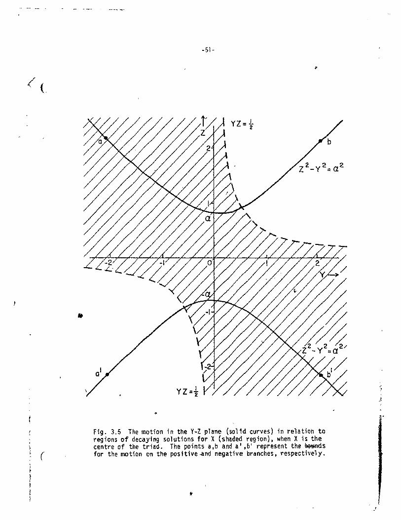
3.5 The motion in the Y-Z plane (solid curves) in relation to 51 regions of decaying solutions for X (shaded region), wh en X is the centre of the triad. The points a,b and a' ,b' represent the bounds for the motion on the' positive and negative brancnes, respectiyely. .

3.6 The response in thé a-K plane when X ;s the centre member.

3.7 Fourier coefficients in Egger's model during period up ta t=5 (reproduced from his Figure 2J. The solid, dotted, dashed and alternating dashed 1ines are associat,ed with the modes (2,2). (1,1), (3,1), and (1,3), respectively.

4.1 The variation of ~ with height and latitude, as determined by Matsuno (reproduced from hi s Figure 3).

...

\

53 \

\{ 59 j

71 , .

\

; t , •

1 '. ~

,1

a

1 •

(:

,"

>

An

81'1

('le"!.'

Do,DI,D" ..., F(x,y)

Fn

In J"( ) )

K 1.:

,;. " M '.

Q

if ~

SO,SI,S':I.

Sen' Tn

Um

X,Y,Z ktl,-ln

t

\ -v 11-

(\

LIST OF SYMBOLS

th Fourier coefficient of leading arder n free mode

Fourier coefficient of nth mode

general inter~ction coefficient

resonant triad amplitudes

external forcing

Fourier coefficient of leadi~g order nth

mode forcing (

initial amplitude of leading order nth mode

Jacobian Dperator

initial conditions parameter for resonant triad interactions

channel wi·dth

resonant forcing

potential vorticity

mean potential vort;city gradient n t ~

resonant tria~ interaction coefficients

modal interaction coefficient

1. Fourier coefficient of leading order nth forced moçle

velocity scale -

normalized r~sonant triad amplitudes

x and y wavenumbers of n th mode

time

) "

,~

i

p c '0

1

c

Ü(y,z)

x,y,z

0('

\. . .,. ~

S €

Âo

.lb

t:

~ (>(, '1, t\

41(x, y, t)

W'~(~}

..w." {jJ,".fff. D 0, 1) :a.

li (

(

, '

! .y i i i-

zonal mean wind

Cqrtesian coord;n~tes in easterly, northerly and vertical directions

normalized initial noise parameter for resonant triad interactiofns

planetary yorticitY gradient

order of resonant forcin~

order of initial ~oi~e

initial noise parameter for modal interacti6ns

aspect ratio

slow time scal e

perturbation stream function t '

total stream -function

linear Rossby frequency of nth

mode

Doppler-shifted frequencies of resonant triad ..

....

"

1 ~ l

~ l

i

" 1

(

,,-,

CHArtER l

INTRODUCTION '

/

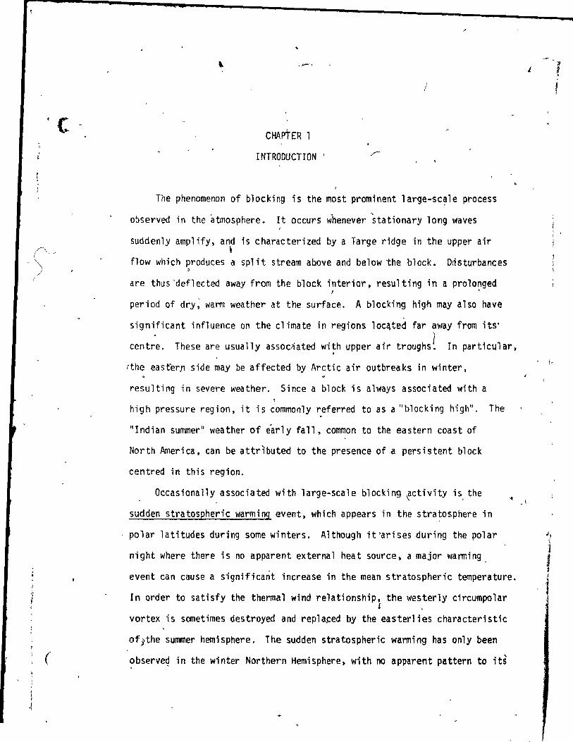
The phenomenon of blocking ;s the most prominent large-sc~le process

obsel"ved in the atmosphere. It occurs w'henever 'stationary long waves ,

suddenly ampl if Y , and is characterized by a Targe ridge in the upper air \

flow which produces a spl it stream above and below the bleck. Dtisturbances o

are thus 'deflected away from the block interior. resulting in a prolo~ged

period of dry; warm weather at the surface. A blocking hig~ may also have .

significant influence on the climate in regions locqted far away from its'

cent;e. These are usually assoc~ated wi~h upper air trOUghS~ In particular.

(the easfer.n side may be affected by Arctic air outbreaks in winter.

resulting in severe weather. Since a block ;s always associated with a

high pressure region, it i ~ commonly referred to as a "blocking high". The

"Indian summer ll weather of éarly fa", common te the eastern coast of

North America, can be attrlbuted ta the presence of ,a persistent block

centred in this regian.

Occasionally associated with large-scale blocking fctivity is, the

sud den stratospheric warming event, which appears in the stra~osphere in

polar latitudes durjng sorne winters. Although it'arises during the polar

night where there is no apparent external heat source, a major warming

..

event can cause a s;gnificant ;ncrease in the mean stratospheric temperature.

In order to satisfy the thermal wind relationship, the westerly circumpolar i .

vortex is sometimes destroyed and replaçed by the easterlies characteristic

of)the summer hemisphere. The sudden stratospheric warming has only been

?bserve~ in the winter Northern Hemisphere, with no apparent pattern ta its

• 1

c

')

~ ~

" \ ,

f ~ ,

J

f , ~

("

, t

Î .'

-2-

1

appearance, and has only appeared simultaneously with the presence of

large-scale tr5"posph.eric block;ng activity. For a more ç1etai1.ed discussion

of major warmings and ttieir pQssible causes, the reader is referred to

Tung )1977).

A blocking situatlon can be a manifestation of so~e instability

mechan;sm, or a resonant response (i.e. the wave amplitude grows linearly

with time) toa surface forcing associated with topographical effects and/or

land~sea differential heating. Recent observations have indicated that the , ~

forcings due to these'latter t~o influences have similar amplitudes, but ~I \;

are 'generally out of phase with each other (Tung, 1977). A shifting of the

relative phase can then lead to constructive or destructjve interference. \

Stnce blocking patterns are usua~ly geographically fixed, this"would seem o

to suggest that a stationary surface forcing is fundamental to the;r

appearance.

A necessary condition for resonance is the existence of a ~resonant ~

cavity", with associ'ated normal modes. "This requires waves· to be reflected

in the meridional direction and at some levèl in the vertical. Energy is

then accumulated in the cavity as waves are forced at ttle lower boundary.

Thus, a polar cap can act as a resonant cavity once southern and vertical

~ reflecting boundaries have been established. It was O~igin~llY thought that \ > •

9

) \ ' 1

the tropospheriC' jet (with its associat.ed large shear) could act as the

southern boundary, resulting in the so-cal1ed J'polar wave guide". However, , o

the planetary-scale Rossby waves are able ta "tunnel ll through this barrier ......

(Tung (1977)}. The recent interest in the dynamics assaciated with , J. "" II

cr itica 1 layers, which are thin "regions in the, y-z plane wh~re the mean , ...

,zonal wind equals the phase speed of the Rossby wave, ha5 led ta the .

o

\ !

(

1

f .

,

1 i l 1 1 \

.

1

t

... • ,

l,

~

t ~,

r ,~' .

i

! ~

r ! \

f 1 • , 1

e ..

(

-3-

concept of the "singu1ar wave guide". This is based on recent ana1ytical

studles which have shown that, given rea1istic atmospheric values of ... viscosity and nonlinearity, the crHical surface can act as the southern

ref1ecting wall. The vertically propagating waves are trapped in the

..,ertical by regions of easterly zonal winds or strong ~terlies, as first

proposed by Charney and Orazin (1961).

These concepts of normal mode~ and resonant cavities are based on '\

linear models and direct resonant forcing. However, because of the 1inear

growth in time, it is c1ear that we cannot continue to dea1 with infinite-

sima1 amplÏtudes. The non1 inearities may significantly affect the ultimate

behaVlOur of a resonant mode. In this study, we shall 'be investigating the

influence of these non1inear interactions on the creation and maintenance

of a stationary, planetary-scale Rossby wave, which can interact resonant1y

with the surface forcing apd produce a large response. ~J

In the literature, Armstrong et al. (1962) and Oavidson (1962) have

investigated nonlinear interactions. in ~asmas. Phi,llips (1960), Benney ..)

(1962) and Longuet-Higgins and Phillips (1962) dealt with nonlinear gravit y

wave interactions. The concept of wave-wave interactions among mixed modes

has been studied by Duffy (1974) for inertia1-gravity and Rossby waves at

mid-latitudes, and by Do~aracki and loesah (1977) for tre var;ous equatorial

types. Matsuno (1971) and Holton (1976) described how wave-mean, flow

interactions "bight possibly tra.wer en erg y ana momentum from resonant waves

ta the up~er jet stream during the onset of a sudden stratospheric warming.

This concept was a1so used by Ho1ton and Lindzen (1972) to account for the

quasi-biennial oscillation of the tropical stratosphere.

( \

r

- ;

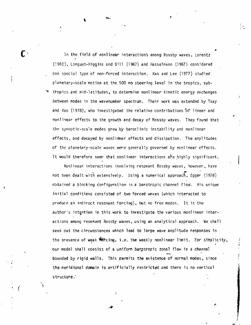
In the field of nonlinear interactionS among Rossby waves, Lorentz

(1960), Longuet-Higgins and Gil1 (1967) and Hasselmann (1967) considered

one special type of non-forceq interaction. Kao and Lee (1977) studied

p1anetary-sca1e motion at the 500 mb steering leve1 in the tropics, sub-

~ t~opics and mid-latitudes, ta determine nonlinear kinetic energy exchanges

between modes in the wavenumber spectrum. Their work was extended by Tsay

and Kao (1978), who investigated the relative contributions 'of 1 inear and

nonlinear effects to the growth and decay of Rossby waves. They found that

the synoptic-scale modes grew by baroclinic instability and non1inear

effeets, and decayed by nonlirrear effects and dissipation. The amplitudes

of the planetary-scale waves were-generally governed by non1inear effects.

It wou1d therefore seem that nonlinear interactions ate highly significant . . Nonlinear interactions involving resonant Rossby waves, however, have

not been dealt with extensively. Using a numerical approac~, Egge~ (1978)

obtained a blocking êonfiguration in a barotropic channel flow. His unique

initial conditions consisted of two foreed waves (which interacted to

produce an indirect resonant forcing), but no free modes. It is the

author's int~ntion in this work ta investigate the various nonlinear inter­

actlons among resonant Rossby waves, using an analytical approach. We shal1

seek out the cireumstanees which lead to large wave amplitude responses in

the presence of weak ~"cing, i.e. the weakly nonlinear limite For simp1icity, , , -';

our model shall consist of a uniform bar~tropic zonal flow in a channel

bounded by rigid walls. This permits the existence of normal modes, sinee

the meridianal domain is artificial1y restricted and there is no vertical

structure .'

, , .

c

. '

(

-5-

'In Chapter 2, the most commonly occurring nonlinear interactions among

forced Rossby waves are described, in the absence of resonant forcing. This

discussion is extended in Chapter 3 to include resonant forcing, in which

we atternpt ta obtain large amplitude responses for each of the various types

of nonlinear interactions. Egger's (1978) results are a1so discussed in

rela ti on to the above ideas. In Chapter 4, the genera l criteri a necessary

to obtain resonant responses in more rea1istic, non-uniform zonal frows are

derived. It will be shown that, ~n general, a resonant mode can grow to a

high level for certain background f10ws provided that the initial free

wave àmplitudes are small enough. This novel concept of the "initial noise

level" wi"ll prove ta ce high1y influential in deterrnining the resonant

response in these nonlinear flows.

l ' , 1

r

t:

•

(

-6-

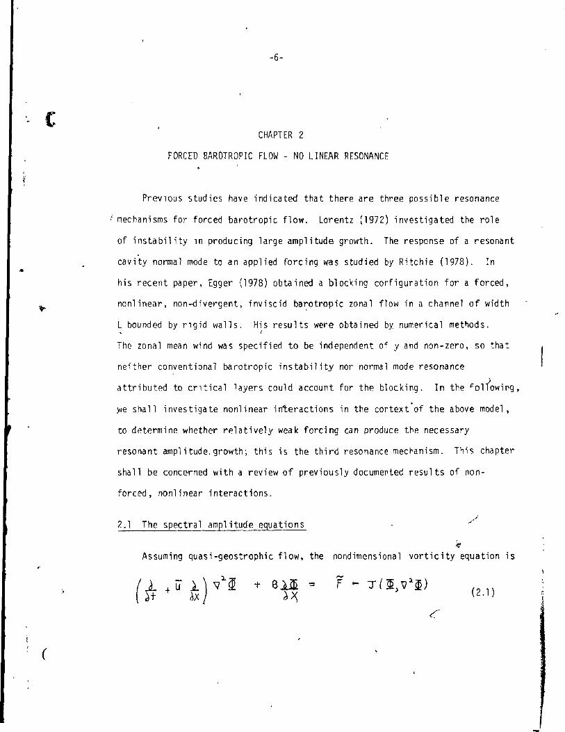
CHAPTER 2

FORCED BAROTROPIC FLOW - NO LINEAR RESONANCE

Prev10us studies have indicated that there are three possible resonance

1 mechanisms for forced barotropic flow. Lorentz (1972) investigated the role

of instability ln producing large amplitude growth. The response of a resonant

cavity normal mode to an app1ied forcing was studied by Ritchie (1978). In

his recent paper, Egger (1978) obtained a b10cking configuration for a forced,

nonl inear, non-divergent, inviscid bar:otropic zonal flow in a channel of width

L bounded by rlgid walls. His results were obtained by. numerical methods. 1

The zonal mean wind was specified ta be independent of y and non-zero, so that

neither conventiona1 barotropic instability nor normal mode resonance

attributed ta crltical layers could account for the b1ocking. In the fodowing,

.we shall investigate nonlinear interactions in the context'of the above mode1,

ta determine whether relative1y weak forcing can produce the necessary

resonant amp1itude.growth; this is the third resonance mechanism. This chapter

sha11 be concerned with a review of previously documented resu1ts of non-

forced, nonlinear interactions.

2.1 The spectral amp' itude eguations

~ Assuming quasi-geostrophic flow, the nondimensional vorticity equation is

(2.1)

c

(

-7 -

- . where U is the constant part of the zonal mean wind and ~ is the perturbation

streamfunction. The total streamfunction,ljI, is related to ~ Dy

\jJ == -uy +~. (2.2)

The Beta pl ane approximation

6 = cJf'I-dy Y:Yo

f -

has been used ta simpl if Y the geometry. The non1 inearities are repr,€sented 1

bY the Jacobian

a.I .L \7:l~ - il. 1. \];r~ = rix V ~). \l(Vl~) d X ày ~y àx

where ~ is a unit vector in the vertical direction. The perturbation velocity

components are related to the streamfunction by

u' =- - ~ ~y

, v' ::; li . dX

The forcing f, assumed steady, is provided by a vort;city source on the right-

hand side and can be thought of as Ci> simpl ified form of direct Newtonian

heating, as suggested by Vickroy and Dutton (l9t9).

In deriving (2.1), we ,have nondimensionalized according to ~J

(2.3)

where "*,, quantities represent dimensional variables. The parameter Um ;5 a

typical velocity scale for the flow.

...

'1 .

(

-8-

':;'!

1t win be assumed that there1is a small forcing, wi.th initial conditions.

consisting of ~"es of. small amplitude (Q(f)). Cyc1ic periadicHy in x is

also impased to model the flow around a latitude circle. This latter assumption,

along with the Eeta' pl~ne approximation, incorporates gome aspects of the

spherical nature of the earth into our model ••

It cil;n be shown that the boundary conditions corr.esponding to no flow

across the channel walls may De written as

at .." = 0,1 (2.4)

provi.ded tha t . • ( i ) œ = 0 at y :: 0) 1 initially

(ii) no mean pressure gradient in x exists

and

( i i i) ~f F cl Y = 0 .

\

)

Here,F is the zona"y averaged forcing. The above will be assumed ta hoJd.

sa (2.4) is applicable. We further assume that F=O at the channel"walls • •

which. together w;th (2.4) and the requirement of zero initial vorticity on ,

the boundaries, impl ies

for all time. It follo~s that a double Fouri'er series representation

;:r;-(' )1::- '=" .( k" X ~ x,y,t ---~An(tlsjn.fnye (2.5.à)

,

or (2.5.b)

;s valid for thls problem and that ,it" is three time'li differentiable in y.,

J i

, , ~ ",

(

(

-9-

The sum 1s oyer all waveyectors,

Tf'le wavevector in (2 .. 5.0} is defined by

where rnand sftare non-zero integers and

f

il :: ..L Llf

(2.6}

(2.7.a,)

is the aspect r~tio. The quantity lx is the zonal wave1ength of the

fundamenta 1 wa ve a t y ~ yo :

(2.7 .'9.)

li

where a is the radius of the earth. /

By defi nition,

mK =-r7' -/\ 1\"

(2.8.a)

while the reality condition for~ results in

B-n :: B~ . (2.8.b)

It also fol1ows by rewr.iting the sin 'nY' term in (2.S.a) in tenns of complex

exponential s that

III

(2.8.c)

In the above, Bn and Bne are the complex amplitudes associated with the

wavevector ~ and the cQnjugate wavevector O. (2.9)

...... -

i 1 1 ,

(

-10-

PC ( ,

The forcing is expanded in the same manner as.!. i.e. •

, {.

F (x,yJ '= )( 2.10)

~" with fn satisfying requirements as in (2.8). Substituting (2.5.b) and (2.10)

i nto (2.1):

? -IK:I~ f ~ + .(.-W;, B"5 e-<~' t - ~ f:. e -i. ~. t ~f " . -!a. ----'" 1· -.<.('l2 of ~~). t

+ L C*>< (-<. k:,)]. [--<. 'K~I";tR;J BiBrn+ e .f,m l

1 ).

,

where •

(2.11)

is the wavevector modu1us, and

(2.12)

. is the dispersion relation for linear Rossby waves. Obviously,..f1!,.. is real and

1l!-o = -.fdn , W"n c ::: 10' n • (2.13)

J App1ying the usual orthogonaliey conditions then yie1ds

<la. +.( .{Un B" = - (!!;; + L C .t", B~ 9: d t - I<i\ 1 a. el""

(2.14)

where the symmetrized interaction coefficients take the form

CntL = Rt)C ~)]~R! ~-1~la)8(~iki+~ ~ 1 nia.

(2.15)

( with 6 ( ) denoting the Kronecker delta.

,

(

, ; ","

~ . ,

-11-

Evidently, C l vani shes if n m

(i ~ t kl+~ =FO

(i;) ~,,~

(iiï) ,KiI:t==IR:I~.

The following relations also hold:

'Cnmm=O (2.16.a)

(2.16.b)

'~ (2.16.c)

(2.16.d)

(2.16.e)

(2.16.f)

(2.16.g)

'where

etc.

Throughout this chapter, we shall consider the initial conditions

(2.17)

Of course, B_n. Bne and B.nc cannot be specified independently, due to the ~

conditions (2.8). Since we shall be dealing with the weak1y nonlinear limit,

we require E"-<I and small forcing. For the -most part, attention will be

l )

f ! }

c.

(

p zno

• 1

-12-

,focused on a few special modes. However, we shal1 soon see that other'waves 0)

which are excited by the initial conditions or the forcing'may have a

significant effect on the flow evolution. One of the objects of the present

investigation is ta examine the role of this "background noise" in the

~ evolut~ geographica 11y fixed di sturbances.

An examinatlon of (2.14) shows that if there is no initial noise

(Ir\=O,Yn) and only a single ~tationary mode is being forced (i .e . .{(J",,= 0,

F,,::/:.O,for sorne n),"then the corresponding solution will grow like t. This

15 the phenomenon of linear resonance. In the next chapter, we shall consider

the amplitude growth of waves when at least one wave is being forced at

resonance. For the moment, we shall discuss the general concepts of various

nonlinear interactions when no such stationary mode~ are present.

2.2 The straightforward expansion

Since it is assumed that there are no linear1y resonant modes present,

the forcing wlll be taken to be of the same order as the background noise,

i.e. ore) , 50 that

To solve (2.14), we expand Bn(t) in a power series in f<:<./:

Sn (t) (2.18)

Substitution into (2.14) and equating powers of E then gives the probl~m

sequence

1

q

)

(

-13-

O(E:) :

The last expression follows from (2.8.b) and (2.16.bl.

",.

The OrE') solution is < ,-"

.' A -.(, (JI' nt B~') (t) -= 0 e + To (2.19)

consist;ng of a 'steady, travelling wave comhined with a stationary, forced ... -

wave which is related to the forcing by oP

Tr\ ;: .( Frl w,.., 1 nl:l (2.20)

Substituting th;s solution into the ()(e~ prob1em g;ves " . ,

(2.21)

Thè first term on the right hand side reprèsents free wave interactions,

and ;s resonant if

and (if Cnlm ;s non-zero)

. Any three free ,waves which satisfy th~ above conditions are common1y referred

to as a resonant triad (not ta be confused with the resonant mode associated ,~"

t " 1

-14-

with linear resonance). Satisfying the above conditions is not a simpfe task.

The existence of resonant triads depends on both the dispersion formula and - , ~~ ~ , l ,

the quantization restr.alnts on the waves. A more detailed discussion of r _..-/

. resonant triads will be presented later in this chapter.

The second term in (2.21) will produce a resonance provid~d that

1JJtl, t ljJ,., :: 0

and

Assuming realistic quantization rules, this resonance condition is more

easily satisfied than that for resonant triads. The details of this type of

interaction will be Giscussed in the next section.

The final term of (2.21\1. involves the interaction of two forced waves to

produce a stationary forcing. This term is not resonant under t,he assumptions

made in this chapter. ~

In the event tha t none of the above interactions result in resQna nc es ..

the solution to (2.21> is

B~(t) =-i ., .If' i.W"t+

+ ~Ae Tm e iWt + -W,,)

-+ Te .... r: 1 . -{U,.,

This result can be used in the O(ë') J crs>· (3) • 'ÇC QJ2!l. + .( {Lf',.. 8" = - ~ -i. L nt-", Clnrt dt /J'

~·,t

,

" 1

i'

c

(

-15-

,-

The first term involves the interaction of free waves. the last involves

only forced waves, while the remaining two are mixfd, involving both free

and forced wave interactions.

The first term is of primary importance. since it is invariably resonant .

whenever tnere are at 1east two waves present. T~s term is resonant if

and

, 1

• (2.22.a)

K' = 0 '1. • (2.22.b)

Any four distinct waves which satisfy these conditions are called a resonant

quartet, which is the higher order equivalent of ~sonant triad. We

will not investigate bhis special type of non1inear interaction any further,

since many of its features are a1so characteristic of resonant triad interactions.

The interacting free waves need not necessarily be distinct; one wave may

b'e int,eracting twice with at 1east one other wave to reproduce itself. Through

such modal interactions, re,sonant termsjare always produced at this order,

and ~an be sho~~ to cause a l'inear frequency modification (Longuet-Higgins

and Phillips (1962) a~d Benney (1~62)). The consequences of this type of

nonlinear in'teracti.on are discussed later in this chapter.

\

2.3 . Freè-forced wave i nteract.iQ.ns r

In t~ last section, we determined that free-forced wave interactions at ,

o (E'lI.) could producé' a resona.nt response provided that

(2.23.a)

.1 1 !

, , "

1 "

po

,

l~ 1 , , ~

" .. t ~ f

! (

• , i , (

~

r 1 r

c;zapq ...

-16-

f

and

(2.·23.b)

where R% is the wavevector of the forced wave. Upon using the dispersion

rel ationship, the above conditions reduce to )' .

- - Km..Y.. a .(2.24)

This can a1ways be satisfied by choosing the initial mean wind correct1y, for

• any set of interacting free·and forced waves.

In the presence of resonant terms at O(€~) due ta free-~orced wave

interactions, t~ solution to (2.21) ;s

The. straightforward expansion (2.18) will th!Js become disordered at large "

times, due t~ this secular terme The series must then be re-ordered in such (li

a way as to l\~),ma;n uniform1y valid for all time, if it is indeed possible.

This is gene~allY accomplished by the method of multiple scales, as outlined

by Nayfeh (1973). The multiple scales approach prov;des for the existente of

,

!

\ i ~ l l l ,

, , J

? 1

, '

a "slow" time scale t' , in addition ta the "fast" t;me scale t. This ,allows ,!

the removal of the secular.terms and results in an amplitude evolution

equatjon for An on the slow time scale~

In the present instance, we require

1: = Et

fram which it fol1ows that

(2.25)

'.

r !

t

(1

•

.d.. ...,. la dt àt

-17 - o

The general amplitude equation (2.14) then becomes

.t

li

Upon substitution ~f the usual asymptotic expanSion and equating powers

the a(E) equa tion i s

with the solution

-F, I~rl

of t '

consistlng of a slow1y modulated travelling wave and a stationary, forced

wave. Using this result in the' O(~ equation yields

f,,). (-l.) \' Il' .. .(.m(t -"-<Un"\" ~ +-<.tlTn 6" =;). LCnh,Ar.. TI"/\ e - dA,. e + non-secu l ar terms. (2.26) èt .e,rn Cft

We consider two free waves and one forced wave, denote~ by subscripts 0,

and 2 respectively, which satisfy (2.23). Sirce other waves transfer their 1\,

energy through higher order interactions, they can be ne91ected to leading

arder. This constitutes a "natural closure" for the system, which seems

more rational than the commonly employed, arbitrary truncation of spectral

models. From (2.26), the evolution equations are ~

(2.27.a)

\

1:

i • J "

\

c.

(

-18-

and

(2.27.b)

Ellmlnating Al ln the above, we obtaln

The same equation a150 applies for Al' This yields solutions of the form

V"'l:' - V'1;'

Ao('t)""'ae +be

where

(2.28. a )

ThlS can be put ln more meaningful form by using (2.15) and (2.23):

[ ;=r, ':l ,.... ,.\ (~~ ,..:r :1.) J'la..

71= lTillk,lo-Koe.l (/K.j -\1<:1.\; IK~I-IKol • rl<~ll ~l "

(2.28.b)

The free modes will grow exponential1y in time 'ifl/iS~eal, which requires

or

Since the inverse of the wavevector modulus can be thought of as a length

scale for the wave, these conditions imply that the forced wave must be of

intermediate scale compared to the free waves for the latter ta graw

exponeotially on the slow time scale. This is a direct consequence of

" Fj~rtoft's (1953) BJocking Theorem, which states that the energy lost (gained)

')

by a wave must be transferred to (from) waves of both larger and smaller scales, .

for two-dimensional. incompressible flow. Here. the non1 inear interactions c

'\

1

!

(

-19-

/

-j

resul t in a transfer of energy from the stationary, forcel wave

to 'the 1ravel1ing waves, which can th en grow. Clearly, the

expansion will become disordered, and we must rescale th"e growtfg'

waves w1th respect to the forcing if a uniformly valid represen-

tation 15 to be achieved. Specifically, the free-forced resonant

tf?rms must be ba1anced by higher order resonances.

To the best of the author' s knowl edge, thi s type of wave

1nteraction has not been previously investigated in the 1iterature.

It is slgnificant ln that it can occur at low arder in the absence

of resonant triads, by imposing an easily satisfied condltion on

the zonal mean wind. The resulting f;rst-order solution takes

the genera 1 form of a slowly modu,lated (in time) trave11; ng wa.ve

moving through a tixed modulation pattern in space. We shall not

t;

consider this type of interaction further. as it does not deal

with ampl jfying stationary waves associated with blocking situations.

However, it cou1d very well provide an insight into thé amplification

of travelling waves, and as such. warrants further investigation.

. '

c

(

-20-

2,4 The resonant triad

In an ear1 ier section, it was shown that a resonant triad consists of

any three waves satlsfying

(2.29.a)

and

(2.29.b)

In the event that there is only a singl~ iso1ated resonance, a natural c10sure

for the syst'em exists, and we can focus our attention solely on the waves

compnsing the triad. The three waves are all assumed to be O(E) initially,

as in (2.17).

The governing evo1utlon equations can be deduced fram (2.21), in the

'bsent of st,tionary WilveS, by'g,in introducing the slow time scale defined

by (2.25) and removing the secu1ar terms at O(E"). This yie1ds the usual '.

triad set:

1 r

\

d& == i (01'1 AI "At d't

clfu = -i.. C:10 Ao "At dt'

.J.II 'C .Ir Jt \.!.!J2... = {. ::tOI Ao A, . d't

Using the resonant triad conditions (2.29) and the definition of Cnlm

given by (2.15), it can be determined that

Cntm

(2.30)

(2.31 )

,,' .

/

(

-21-

where n,land m are distinct sub5cripts, and

o ~ U~R! 1< K'r 1- K: JI K! + ~Kf!)] [(ko<O",--k',<u.)+(k,W"1.-k':I<l!i )-+(!u-(O;,- t:o~Ü lK:tl~tl~i 1 9 <3 1<'0 k, k'l.

~ (2.32)

15 a constant symmetric with respect ta cye1 ic permutatons of the three p

lndices. From (2.31), we see that the relative signs of the interaction

coeff1cients are determined by the relative sign5 of kO

' kl and k2. From '\.,

the co~dition (2.29.a), the x-wavenumbers cannot be of the same sign; hence

the same result must hold .for the interaction coefficients. This restriction

on the slgns Dt the interaction coefficients will be shown in Chapter 3 ta

play an important role in 'resonant triads having a l inearl·y resonant mode.

If we use the transformation

and define the Doppler shifted frequency

the amplitude equations (2.30) become

where

d....Ik =: -t 5 Wo D D,~ D'4" d't

J t'\ • S .Jlf"° "'0'" DI" ~ == 0( "W:l Vi

d't'

s=- - D

6 1 ~Il KfIlKtI

• (2.33.a)

(2.33.b)

(2.34.a)

(2.34.b)

-

---~----.--~~-----_ ... ----~--------------~-- -----

(

-22-

For convenience, we define

(2.34. c)

The constant S is again symmetric wlth respect to cyclic permutations of the

three indices, and the three interaction coefficients can be shown to sum ta

zero. In this system, the interaction coefficients ?re proportional to the

Doppler shifted frequency, and tO"I;\ represents the actual energy of the

nth mode. This is the form used byJ1asse1mann (1967) to show that the mode

with the highest Doppler shifted frequency magnitude is linearly unstab1e '

with respect to smal1 perturbations. We shall work with this form, as opposed

to the original set (2.30).

Equations (2.34.a) may be solved analytically in terms of Jacobi e1liptic \

functions, as shown by Bretherton (1964). It turns out that the solution

is perlodic, with the three triad members simp1y sharing energy among them-

selves. If a second resonant triad were to exist having a member in common

with the original triad, ener~y could be shared between 'the two set~via the common member. This possibility shall not be considered here.

It remains to determine the existing triads. Using the dispersion \ Co

• relation and the resonant triad requirements (2.29), it fol1ows that

(2.35 )

Once pairs of wavevectors are determined from t~e above, the third member

of each triad can be found byapplying (2.29.a).

This situation was examined from a different point of view by

\

(.

-23-

<;

Longuet-Higgins and Gill (1967). They pointed but that the wavevector

requirements for a resonant triad can be written as

. , -=J ~ 4 ~

so that the ends of the four vectors KI , K:I., - KO and 0 form a parall elo-

gram whose d; agona l s i ntersect at - 1 R:I/~. They then def; ned a wavevector ~

such that

(2.36) 1

sa that (2.29.b) is"satisfied for any choice of Ki . 1 This was substituted

into (2.35) and simplified through the use'of polar coordinates:

(2.37)

where

(2.38)

... After a considerabl e amoùnt of algebra, they obtained

(2.39.a)

where

(2.39.6)

with

(2.39.c)

Once a particular K:, has been chosen, specifying IRtI and 1\ by (2.38) and

(2.39.c), then I~I can be found as a function of r/;!, by using (2.39.a) and

( . ) ,~ ~ 2.39.b. This results in values Q'I K.3 which can be used albng with

• l

, ] t

1 •

..

/

i . l

(

-24-

. ~ ~ f in (2.36) to determlne KI and Kl. . It 'follows that the quartic curve

obtained from (2.39.a}gives the locus of pairs of wavevectors which form

do \ :-'tkor resonant triads with Ke . One will obtain different curves by changing

or ~o , or both. Some ex~mples of the curves obtained by thlS method are

i11ustrated in Figure 2.1. The geometry of the flow has been specifled so

that ~C:-S: , fram which it follows from (2.6) that a11 wavenumbers are integer

multiples off!'. We have also fixed ~o= t'3Sowhile varying ~ such that f~f'=-

171f, SOr( and Q711"l. for the three curves with centres denoted by Pn , PSO

and P97' respectively. In the diagram, the 'resonant triads are determined by

any two diagona11y opposite (through the centre- Kl/.l1r) points on the guartic

curves which passess integer coordinates. These points are indicated by their

wavenumber coordinates, (divided by 1( ) and form a parallelogram with the ~ ...,.

vectop -Ko and 0 , as expected. Evidently, the wavevectors (-5,5), (4,-9) . and (1,4) form nearly an exact resonant triad for this geometry (in the sense

that (2.35) is satisfied within ().Ol%), a fact which can be verified numeri-1

• cally. For more i~ormation, the reader ;s referred to Longuet-Higgins and

Gill~ 967).

I~ the next chapter, these previously estab1ished results shall be

extend~ to include resonant triads having one member forced lat resanance,

with~ome interesting cOnsequences.

2.5 Modal interactions .,

If no resonantes occur at cie' in the straightforward expansio~, then

attention must be shifted to the next arder. Assùming no resonant quartets

are present, the OUjequation can be written as

1

(.

(

-25-

15

t " l-

TT

10

(- 5, 5)

'" -10 -5

K --TT

3

Fig. 2.1 Locus of pairs of wavevectors k1 and t which form a

resonant triad with ka for 11=O.5, <1>0=135°. and l~o~2/1T2=17 (curve , ). 50 (curve 2). and 97 (curve 3).

(

, (

-26-

/

We can then determine the governing evo1ution equations by introducing the

slow time scale

(2.40 )

and removing the secular terms. This leads to equations of the form

(2.41.a)

where

(2.41.b)

In (2.41.a), the sum extends over positive and negative wavenumber components

ln x and y. However, according to (2.8) and the leading order solution (2.19),

It is thus convenient ta regroup the interacti~on coefficients associated with ~

these four modes into one general interaction coefficient associated with IAt/. The sum in (2.41 .a) may then be written as a sum over non-negative integers:

" where

J" • N 5 !4 CUl..O = --tAn l b IAel dt' ~o ~

(2.42.a)

Sel' = 4 L 2: f"'· ... ClhPk ) (2.42.b) ".. p",~-e, (~_e.c {Or. +W-p t ".

is the interaction coeffici~t associated with An ;nt~racting twice with AL

to reproduce itself. In this analysis, N+I waves are being considered.

Using (2.16.a) and (2.16.e) in the above, we obtain

1

(

-27-

This should be immediately obvious due ta the nature of the Jaçobian. which

disallows any wave self-interaction .•

Upon mu1tiplying (2.42.a) by An* and adding the result to ni .comp1ex

canjugate: :4

- Ji/AnI = 0 "In. d't

Since the initial conditions (2,17) and the leading order solution imp1y

it follows that

1 An \':1.:: 1 ~1':I.::2 con~t (2.43)

The solutions to (2.42.a) are then

(2.44 )

where , (2.45)

is a real constant containing the inf1uence of the initial noise. Combining ~

(2.19) and (2.44), we see that ta leading order,

sa that the total frequency Wn for the non1 inear probl em i s given by

\

\

) ..

( l

-\ ,

-28-

Thus, the nonlinear terms act ta drive the wave off its linear frequency by an

amount

Ân el.

referred to as the nonl inear freguency shift. It will be small for E<:,( l, but

may still have a significant effect. Furthermore. it is strongly dependent ,

on the initial noise level. An impo{tant consequence of this behaviour, which

shall be discussed in the next chapter, is that a wave being forced at

resonance may be driven off its resonant frequency by the nonlinear inter~

actions of other waves. Thus, this mechanism can clearly inhibit resonant

growth, especia'lly if the initial noise level is large.

'1

, , ! " .

F (.

( ,

•

•

-29-

CHAPTER 3

FORCED BAROTROPIC -FLm~ AT LINEAR RESONANCE

The previous chapter was concerned with nonlinear wave interactions

in the absence of linearly resonant forcing. It was found that a variety

of interactions were possible, depending on the frequency an~wavevector

relationships among the participating waves. Of these, only the forced­

free wave interactions tesulted in a large response (defined as the modulus

of the ratio of the free wave solution to the forcing). For resonant

triads a~d modal interactions in the absence of resonant forcing, we found

the response to be 0(1). Our aim in this chapter will be t~ investigate

resonantly forced stationary waves. q

According to the dispersion relation-

ship (2.12), these modes satisfy

(3.1)

which reduces to a condition on the zonal'mean wind once the geometry of ,

the flow is spe~ified. As in Chapter 2, the weakly nonlinear approach will

be used; this Wlill be foûnd to require both smalT initial wave amplitudes

. and forcings. Resonant triad and modal interactions shall be studied, and

the conclu-stons applièd to Egger's (1978) mmerical results. In particular, -the effect of the initial noise level shall be examined for each typè of

interaction.

1 1 1

L , 1

-30-

3. l The straightforward expansion

We are interested in obtaining solutions to the spectral amplitude

equations (2.14) in the weakly nonlinear limit when stationary modes are

present; the procedure is as outlined in Chapter 2. The amplitudes are

expanded in the usual power series, substituted into (2.14) and powGrs of

~ equated. It;s first assumed that the forcing is of the same level as ... the initial noise, i.e. 0 (E), with the usual initial conditions (2.17)

being used. For clarity, the resonant and non-resonant modes will be •

designated by subscripts n and p, respectively. This yields the following

set of equations at the lowest orders:

. (3.2) ,

*1) _ ~ C B II14:S

lt1•• djl2J . 11'1" B (~J - ~ r cf.J4a(I). - L "em e "', + -!.Ulp P - L.,-pllflDC. l1l'I {3.3} t ' -i,rt') t ~ /YI,

o (e'):

where the forced component T pis de fi ned as in (2.20). " -­v '

J

,-, ,

•

1 1 ,

,

i 1

~ 1

f

(

-31-

If Fn:#O and there i s no background noi se or forci ng in other modes:

A p = Fp = 0 't/ P

then the ser i es termi na tes a nd the complete sol ut ion 'i s .

. , Br (t): 0 V P .

On the,other hand. free travelling waves and non-resonant forced waves will

normal1y be present in the actual atmosphere. sa this case is hardly

real istic.

Ih the presence of background noise with one resonant mode, the

expansion for the perturbation streamfunction can be shawn ta go as

Evidently, the expansion becomes disordered at large times TNO(€-').

and the fundamental and its harmonies are seen to grow to the level of the

~ean flow. At this point. the flow becomes fu1ly nonlinear and weakly non-

1inear theory no longer applies. To make analytical progress. it is '. ty,

apparent that the forcing must be assumed smaller ~han the initial noise

level.

The choice of the forcing wil~ depend on the type of nonlinear inter­

action being considered. It will be determined by requiring that the

resonant growth due to forcing and that due to secular nonlinear interactions ,.

appear at the same order. If we define () ta be the order of the forcing,

it is clear that a=€~ for resonant triad interactions and J= €'"

(

-32-

for modal interactions. The resulting evolution equations for these two

types shall be considered in the following two sections.

Flnally, it should be mentioned that even if there is no direct

resonant forcing (F"t o) , resonance may still appear at 0 ({l} due to

the interactions of other forced modes. This is the situation considered

by Egger (1978); it will be discussed at the end of this chapter.

3.2 The forced resonant triad. ~

From the resonant triad conditions (2.29), i~ c~ easily be shown that '

al' three waves must be stationary if more than one ~tionary mode exists. -f

In this event, there are two distinct possibilities. One of the triad

members may have a vanishing zonal wavenumber, in which case the resonant

triad represents two waves interacting with a vanable mean flow. \~e shall

not be concerned with this possibility, as it does not involve energy

exchanges among a wave triad. It;s a1so conceivab1e that three stationary

waves satisfy (2.29) and hence are forced at resonance. This system does "

not appear to lend itself to a simple analytical approach, and requires an

additional restriction on the wavenumbers (the wavevectors must define an

equilateral triangle in wavevector space)_ Hence, we shall consider a

resonant triad cons;sting of ~ stationary mode only. The resonant mode

shall be denoted by DO and the travell ing waves by Dl and O2, The usua1

initial conditions are assumed:

On ('(=0> =In ; n::.o,',~.

...

-33-

. ( ) Us i ng cf:J e~ , cr= Et and the resu lts of Chapter 2, the resulti n9 evo1 ution

equations 3fe

D," D~" d.Qg = .( 50 - M d'C ciJh :: -i... S, Do .... Da ... (3.5) d1;

~= { S If' * ::l Do DI dt:

~ 0

where

n ': 0, I,~

------.. as in (2.33.a). The interaction coefficients are defined by (2.34.b) and

(2.34.c), while the forcing at this arder is given by

(3.6)

, It can easily be shawn from the evolution equations that there is no

direct energy exchange between waves having the same sign. Moreover,

Fj~rtoft's (1953) Blocking Theorem indicates that energy transfers must

proceed via the wave of intermediate scale. with energy flowing into or out

of this mode fram waves of larger and smaller scales. ,Hence, the triad

member having the different interaction coefficient sign ;s a1so the wave of ------\~

/intermed;ate length scale. It also has the largest Doppler-shifted

( frequency adcording to (2.33.b) and (2.34.c), as noted by Hasselmann (l967).

The wave of di fferent 5 i gn will be referred to as the "centre" o,f the tr i ad. ,

(

while the othe~two modes shall be called the "w;ng members".

•

i i 1

i

l 1 l , 1

i , ï î j , !

},

,

1,

(

, i ~

~ ( .1

... UJ ; ...

------

-34-

From (3.5), we have

.lJ2J? = S,

eonn-. (3.7)

Since E~ ~ lonra represents the energy of the nth mode and from (2.34.c):

S = Const.

then the quantities in (3.7) are proportional to the action, defined by

(3.8 )

Hence, (3.7) împlies that both the sum or the difference of the actions

of the two free waves is conserved, depending on whether S, and S2 are of . opposite or similar sign. If S.5:1.<0) the sum of the actions is a constant,

1

sa that the action in each mode is bounded. Without any loss of generality,

we may then define Dl as the centre of the triad. An energy transfer

diagram may then bé u~ilized to describe energy exchanges among,the triad

members, as illustrated in the top of Figure 3.1. From the form of the

amplitude~quations (3.5), it is evidently difficult ta transfer the energy

in DO (due to the for~ing) into the free waves unless there is SUffiCien~ energy in O2, If the initial noise level is small, tQis energy transfer

will be impaired, and we can expect the forced wave to grow to large

ampl itudes. Thus, the initial noise level appears to play a significant t

role in this case. In the case where SIS~70, it is the difference of the

actions which is a constant, sa that the action in each mode is no longer

necessarily bounded. In this instance, we can define D2 as the mode having

--~ -,,--..

,

, ....

-35-

FORCING

. D,

FORCING

Fig. 3.1 Energy transfer diagrams for a resonant triad when the forced mode ;s a wing m~ber (top) and the centre (below).

, ; ;

1 1

j 1

i i

1 ~ ,

i ','

(

-36-

( the larger lnitia1 action. i.e.

The associated energy transfer for this case lS illustrated in the lower

part of Figure 3.1. One would anticipate the forced wave growth to'be

limited somewhat since it can give up its energy easi1y ta the free waves.

Furthermore, the initial noise level'might nct be expected to be a signifi-

cant factor here.

The equation set (3.5) does not appear to possess an explicit closed

form solution, unlike the non-forced set. However, we can obtain sorne

va1uable information about the resonant response under certain limiting

conditions. If we introduce the substitutions

and

~j7

Do:' ooe ,

.irt M = me

> .i(l}-t)

D:I.=Q:.l.e

in (3.5), where 1 is any constant, then it is easily seen that aO' al

(3.9)

(3.l0)

and a2 will rema;n real if theyare initially sa. In the ensuing discussion,

we shall consider this special case. If;5 important to keep in.mind that

ao' al and a2 are permitted to take on negative values.

Substituting (3.9) and (3.10) into {3.5} yields

, )

\ i

1 3

f , ,

(

(

.... ---- ~-~ ----..--...----

-37 -

d...1L. = 5;', Qo Q:.. dt"

dJh::. ç:l, QoO, d't

while the integral constraint (3.7) becomes

co ",sT. .\

f

(3.11~

(3.12)

If we regard aO' al and a2 as the Cartesian coordinates of a particle (phase

space), the equatiDns (3.11) govern the motion at each point. In addition,

the constraint (3.12) ~estricts the trajectory to lie on a certain surface,

determined by the initial conditions. If aO

;s the c~ntre of the tri~,

S,S::\.)o and (3,12) becomes

Q:l.:I IS:d

~ = c':l Isd (3.13)

which defines an hyperbola in the al - a2 plane.' Converse1y, if aO is a

w;ng member, S,S" <0 and (3.12) takes the form

aL -r ~ :: C).

IS:l.1 \ 1 S"d (3.14)

which is an ellipse in the al - a2 plane.

We now proceed to an exam1nation of the stationary solutions to (3.11)

and their stabil ity. Evidently, the steady solutions are

00 = 0 ., (3.15)

The 1; n,earf zed equations then become

, !

'" 1

)

,

" 1

(

1 f-i

~~~--~~--- -- ---

.. -38-

-, - 1 50 Q,a~ + $0 a~ Q,

dJh.' == ~t Q ~ Q 0 '

dt

which reduce to

- m

(SoS~ a,'a + SoS. ëf~"l.) aD '.:: 0 .

QI

Hence, the system is unstable if

If aO is the centre, both SOSl and 50S2 are negative, 50 that the steady

solutions are always stable. If aO is a wing member (with al being defined

as the centre), then SoS. ~O, S~ Sa 70 and the condition for

instability becomes

(3.16)

"-

This indicates that the action in the wing free wave must be less than that

in the central free wave for instability,as proposed earlier. As QI 70, ~

this reduces to Hasselmann's (1967) criterion for the instability of a

non-forced resonant triad.

1

!. i •

1

(

(

-39-

Essentially, there are four parameters for the problem, namely the ./ .-/-

three initial amplitudes and the forcing. The forcing dependence can be

eliminated by normalizing according ta

where

E;!. = i,m ; 0( = ...c.. 'Sol/S,Soll'l... E

so that the evo1ution equations (3.11) become

with

d.X= dT

$'0 YZ -.J. ~

.dt. = s. XZ dT

.dL::: $,. XY dT

5,,- Sg"~n.

The integral constraint (3.12) simplifies to

,

• •

(3.17)

(3.18)

(3.19)

(3.20)

(3.21 )

To determine the motion in phase space, we shal1 consider separately the

two possibi1ities for the sign of 5,S2:

(i) Forcing in a wing member

If the stationary mode (X) is a wing member, while Y is taken

as the centra' member, then S,Sa <: 0 and (3.21) takes the form

1

\

(

-40-

Y:l z;l. l. + .::. 0<. (3.22)

or

z = of- / o<~ _ y.l . 1 /"

The Z sign indicates that the correct branch must be chosen for the square

root. Using the above resul t and the first two equations of (3.19) gives

+

Upon integration. this leads to

(3.23)

In the above,Cl( involves the initial noise,(normalized by the forcing),

Whlle the initial values of al1 three modes determine K . . Before proceeding to an analysis of (3.23), it will be instructive to

determine sorne preliminary information about the motion. For convenience,

we shall take Sa to be positive in (3.19); the qualitative behaviour will

not change if it is chosen negative. It follows from the first equation

in (3.19) that the rectangular hyperbola in the Y-Z plane,

(3.24)

separa tes the region where X is increasing with time fram that where it is

decreasing. There is no growth alon9 ·the"above curve. However, we a150

know from (3.22) that the projection of the'motion onto the Y-Z plane ;s a

, ,/

(

-41-

circle of radius C<. The situation is then as illustrated in Figure 3.2.

For CX'< 1 ,the motion lies total1y within the region where X is always

decreasing at a finite rate with time. Evident1yX~-C:Oas T~ ~ and

we have unbounded growth. If 0(=1, the circle and rectangular hyperbola

intersect at the two points

and the motion may or may not be bounded, depending on whether X:: 0 at

these intersection points (the steady-state solution). For r:J... "/ l , there

are four tntersection points which separate the positive and negative

tendency regions for X a10ng the projected path of motion. From the above,

it is clear that a sufficient condition for unbounded growth is 0< é.. 1

To determine whether unbounded growth exists when rX.. > l , we now consider

(3.23) indetail.

It will be convenient to work with the quantities

(3.25 )

and x2, instead of X and Y. Equation (3.23) may then be written as

It can also be shown from (3.19) that ,

~ j

(

, ' , .

-42-

Fig. 3.2 The motion in the Y-Z plane (solid curves) jn rel~tion tg regions of decaying solutions for X (shaded region), when X ;s a w; ng member.

-43-

(' 1

~ Combining these two results yields

(3.26 )

... where

(3.27)

From (3.23) and (3.27), the initial values of p and Y are/relôted by

. -1 ( Yo / ) , po ::: ± SoS • n 1 0<.

and we can restrict Po ta the principle branch of the inverse sine function:

\

We can regard (3.26) as an equation of motion governing thê trajectory

of a partiel e, with p representing its dJsplacement. S-inee the ,left-hand

side is non-negative, the motion will be restricted to values of p sueh

that f(p)~o. Evidently, f(p) is bounded by the curves

g.(p)= I<+p

and fl f (p) -1 :!: 00 CI s P -T ± 00 •

We then have the following possibil Hies for f(p}, assuming 0<."'1' ,as

shown in F'igure 3.3. If fep) has only one zero in thè region Ipl~ t-(or remains positive in this region), ·the motion is restricted to the right

of this root. With larger values of eX. ~ for a given K, two more zeroes

(

(

/ /

, "

-44-t _

t( p)

t t(p)

/ /

/ ~, / \).').

/ ~'" / Il 1

~ f(p)

/ / ')., / ~~

/ ~

/

'" / '"

lT

/ /

4

7 /

/

lT

2" p~

/

/

/

/

/ ~'" Fig. 3.3 The thrcc po-ssihlc fonns of f(p) when ft;'>". \'lÎth (ll':: a2~ <13_'

The clilrk curvcs r'cprcscnt t~c p(~rmitted motion, ~/hile the dashed ".,. It"ti .'~. tl\,. "'" .• ~./I' t/ll' ~

- ' . ~

-

t 1 i i , .J

1

\ .' 1

i i j .

f ,

'. ,

, '.

\ , .

, .

-45-

may appear;n Ipf ~ ~. The motion ;s then either contained in the

region bounded by the smaller two roots, or restricted ta the right of

the'lèlrger root. for even greater values of o<~ ,there will onlY be two

zeroes in the interval and the~otion will be bounded. Let us ,denote a

~ given root by p. Local1y, (3.26) becomes .. ,,~ 't!

wHich integrates to give

(p_ p) l'V

for large T. Evidently the particle is reflected by the zeroes of f(p), c - •

since (p - p) has the same sign as f'(P). Thus ,the motion will be unbounded

if the particle is restri~ted ta 1 ie to the right of the largest root in

1 p 1 ~* . For the case represented by the middle diagram, the initial ....

values of p (hence Vo) will determine the rest~cted region .. Finally, we " ,!

note that for K small enough, f(p) will be negative for a given 0( for a11

r pl ~ f ; this is not allowed a~cording to (3.26). " Hence, the

permissable values of K are larger than a critical value, which depends onlo(.

In ~ region of interest

can be shown to occur at

~ 1 P 1 ~ ~ , the rel ative extrema of f(p)

-1 -1-)'-.! .J. coS (0("

J

~

with the plus sign corresponding ta a minimum and the mi~U~S;gn' to a

maximum. For 0(.( J ,the "function is monotonically increasing, implying

unbo~nded solutions as argued earlier. A lower bound for K wh~n 0< <

1

(.

is found by rf!quiring

-46-

f(~J 2 0 ,which from (3.26) leads to ~

When tX= l ,f(p) is monotonicall~ increasing. Hence, there will be an

unbounded response unless f(if}=o, in which case the particle can De

shown to becornt:! "absorbed" at the root (the steady-state solution). From

{3.26), this requires

kc t"" = J) :: ± -*' ...... -O. ~ 85. (3.28)

For ex), , the lower bound. of K ois determined by requiring f(p",Qllu 0

This condition can be obtained with the aid of (3.26) and the expression

for the rel ative maximum. It i s found that

.,

'" Bounded solutions are possible if f(plI\'I\)~O ,for which (3.26) and the

expression for the relative minimum give

1

Final1y, in the overlap region k', (II() < 1< < K::s (rit,) • the response may be

either bounded or unbounded (depending ton 'the initial value of Y). These - d

various regions are illustrated in Figure 3.4. The dividing curves k,(~) '.j K~(O(.) and \('3 fod intersect at the triple point Kc defined by (3.28),

~ ,

which iS'lcharaçt~ristic of the steady-state solution. According ta (3.22)

and (3.23), keelting the initial noise con~tant whi1e varying XO' the initial ~ (

l ' 1

!

1

l , } 1 (

, , "

(

-47-

____ "'2 X = 3-0

___ -~ ..... 2 X = 2·5

.... 2 X = 2-0

Î K

~ ____ ---_80UNDED .... 2 X "1,5

RESPONSE

rr----- _~ __ ..... 2 X = 1-0

-3

Fig. 3.4 Th ' In the th" e respons . val 1n hatched e ~n the a-K l are Ile Qf Y. The li reg10n, the r/ ane when X is . a 100 ; nd ; c. ted . ne s 0 f co ns ta nt s ~~nse i s depend:n ~' ng member. sponse in the b on the initial ounded reg' 10n

i

1 1 ,

. '

..

•

, i \ t 1

1

$ P :#

-48-

ampl itude of the re,sonant mode, is equivalent to varying K with 0< constant.

From the diagram, it is clear that for any 0< , there exists a ·value of K

sucf't-, that the response becomes unbounded. This is not too surprising since

the effekt of the nonlinearities can be shown to be small in this limit.

Similarly, decreasing Zo with Xo and Va held constant is essentially' the

same as decreasing O(with K fixed, and will eventually lead to an unbounded

response. Hence, the amount of initial energy in the wing free mode is , crlJc;al in determining the resonant response, as was indicated by the

earl ier stability analysis.

For values of 0( and K in the bounded response reg;on, we may a1so

determine the maxi~um response in the following manner. The relative maxima

for X will be given by

and

dX :: 0 dT

,..., at X=X.

From (3.19), the first condition requires

and ; t may be shown tha t

N ,...,

The values of Y and ,2 may be detennined by solvmg (3.22) and (3.24)

•

1 ( ..

r,

{ f

simultaneously, which leads to

and

?='!o([1 ?â

Z=ZA-[I fi:

The maximum response occurs for

-49-

+

+

V 1 ~ o<.-~] Il,,

v -~ ] -Ill. 1 - lX •

tv:l _~ ,...,

• y -2 <0 . X ) 0 ) ,

and can be shawn from (3.23) to take the form

(3.29)

X~ (<<, k) = k - ~"[ 1 - VI - o(-~ J + 5Î ~ Tf I-J~-o<.-' rl (3.30)

The lines of constant response ln the bounded motion ~:g;on are plotted in

Figure 3.4; theyare nearly parallel to the li~s Of constant K. The maximum

response is evidently directly proportional ta K and inversely related to~.

It appears that the initial noise level is the significant parameter for the ~ ..

resonant response only forO(~I. Whenot)l, it i5 the initial amplitudes

of the resonant mode (XO

) and the wing free wave (Zo)which determin! whether

the response i s bounded or not. Furthermore, Xo i 5 the critica l parameter

for bounded responses.

As a sidel ight, we recall that the steady-state solution for 0( = 1 ~:;L

required X = 0 , or us;ng (3.30):

which is in agreement with (3.28).

•

--

"

-50-

(ii) Forc;ng in the centre member

If the stationary mode is the centre of the triad, Sr S::t ') 0 and

(3.21) becomes (3.31)

or Z := t. J 0( ~ + y::t

i'he particular branch ;s fixed by the initial condltions, since Z can never

go through zero. Let us first consider the motion in the Y-Z plane.

According to (3.31), the particle mpves along one branch of an hyperbola,

specified by the initial conditions. The rectangular hyperbola

YI = s~ once more separates the reg;on;n the Y-Z plane whe,re X is increas;ngjlith

time from that where it is decreas;ng. For a given branch, the two curves

intersect at one point. These concepts are i11ustrated in Figure 3.5.

Proceeding in the same manner as in case (i), we obtain the second

i ntegra1 constra i nt

X:l + y;l.:: :tSo sÎnh-' (YI d() + 1IfK ; lX. =1= 0 (3.32)

or

where ~ X:l + y~. r" ==

It follows that

f1f=) ~ =- p ,. • t~

D( SInn p (3.33)

p== r'-- K . . /

Equation (3.32) impl ies

..

o

..

(

- --~- ~ ---.,-v-

-51-

l'

YZ=t

fig. 3.5 The motion in the Y-Z plane (sol id curves) in relatioh ta regions of decaying solutions for X (shaded region), when X is the centre of the triad. The points a,b and al ,b' represent the OOttnds for the motion on the positive .and negative branches, respectively.

--'

(

-52-

so that Po is no longer restricted to a particular interval. The derivative

of f(p) vanishes at the point

pc = t si nh-' ( ~) corresponding to an absolute maximum. Hence, we require

for (3.33) to be consistent; thtis constraint reduces to

in the c(-K plane. Since (3.33) indicates that

as p ~ ± 00

the permitted motion must be bounded. These results are i1lustrated in

Figure 3.6.

(3.34)

The maximum possible response can be determined by the same,method as

used in the previous problem:

.1(' (0<, k) = k - ~' ~I t 0(' - 1] T Sinhn kt~" -In. (3.35)

The lines of constant response are included in Figure 3.6. We again find

that the maximum possible response is directly proportional to K and inversely

related to 0(. By taking ex. to be constant, we see that Xo determines

the response for large 0<. , but is not ;'mportant when 0< <<: f. As 0< approaches

zero, it can be shown that values of Y and Z become restricted to one

quadrant of the Y-Z plane, and that an unbounded response win resul t if ...

(3.36)

t, ~

{ • l' r,

•

~ ~ "

p

(

LA_

-53-

3 -2 X =3,0

..... 2 X =2·5

2 .-w2 X =2·0

i BOUNDED K ..... 2

X = 1·5

RESPONSE -2 X = ',0

.... 2 X =0,5

-2 , 1

~ " 1

-3

Fig. 3.6 The responsé in the a~K pla~ wh en X is the centre member:

1

1

(

\

p UJO<1QS

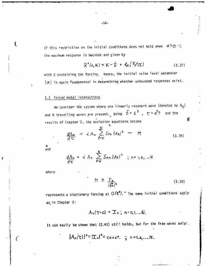
-54-

If this restriction on the initial conditions does not hold when o<.=-O~'

the maximum response is bGunded and given by

(3.37)

with E containing the forcing. Hence, the initia' noise level parameter

(0<) is again fundamental in determining whether unbounded responses exist.

3.3 Forced modal interactions

We cDnsider ttie system where one' inearly resonant wave (denoted by AO)

and N travelling waves are present. Using 0' = €"3 , ~

l:' €T and the r ," ,

results of Chapter 2, the evolution equations become

'III and

where

N .,

.{ A 0 L 5(0 IAt/"l t=o'

M

~ 1"\= t,;l, ..• N

(3.38)

(3.39 )

represents a stationary forcing at 0 (€1). - The same initial conditions apply

as .. in Chapter 2:

It can easily be shown that (2.43) still holds, but for the free waves on1y: ,

; n = \,~, ••• N.

8 _

"

,

j

t

-55-

Hence, (3.38) may be rewritten as

(3.40)

where ./\0 is given by (2.45). This can be ;mmediately integrated to give

• ..<: Ao 't' Ao('l)= -~ + ce

..1\0 (3.41 )

consisting of a stationary component and a travelling mode of frequency

(3.42)

on the fast time sca1e.

The effect of the initial noise, which is contained in the factor Àe

is to produce a non1 inear frequency shi ft (defined by 3.42) off the

resonant frequency of the stationary mode. Since e is small for the weakly

\, nonlinear theory, this shi ft requires a significant amount of t;me to

influence the ampl itude growth. Once the nonl inear effects become important,

the stationary mode will achieve a maximum amp1itud~, which involves the

factor 1 H/.Àol . This value ;s essentially the i~~erse of 0(

defined in the prev;ous section. Hence, the resp6nse ;s again inversely

related to d.. , and will ,be large, but finite, for small cf.... If the

resonant forcing is detuned hy an amount equal to the nonlinear frequency

shift, it can be shown that an infinite response will be obtained. Thus.

since modal inter.actions are not,required to satisfy imposed conditions

(as was the case for resonant triads), they are more 1 ikely associated

with amplifying planetary waves • . These concepts agree quite well with Labitzke's (1978) observations

"' \" " •

p

(

(,

1

CUQ

-56-

of the planetary-scale zonal harmonic height waves during a winter w~en the

sudden strataspheric warming appeared, as opposed to a winter where it

didn't. A major warming was found to occur only when height wave 1 reached

a maximumamplitudewhilé height wave 2 attained a corresponding minlimum,

in bath the troposphere and stratosphere. The results for the baroclinic

problem should not differ qualitatively from those of the simpler barotropic

case. rt follows that the occurrence of the sudden stratospheric warming

is apparently contralled ta some extent by a large average value of the zonal ,

mean wind (necessary for stationary, planetary-scale waves) and a small

initial noise level.

3.4 Appl ication to [gger's model

The nonl ;near interactions of forced waves and slowly moving free waves

in a uniform barotropic flow were studied numeriçally by Egger (1978), in

the context of ~ fully nonlinear, barotropic model. He attempted to deter­

mine whether particular configurations of forcing could produce a blocking

pattern. One experiment 'he eonsidered involved inviscid flow without wave­

mean flow interaction :'in a channel of width L bounded by rigid wall s.

,The forcing was defined as a vorticity source, and the wavelength Of the

fundamental wave was chosen to ~e

which defines the aspect ratio as «=0.5.

Basic"ally then. his model corresponds to that presented in the first

section of Chapter 2; the initial conditions, however, are quite special ..

Egger prescribed his initial conditions 50 that two forced standing waves

•

! t

t

f'·

• p

r

co

-57-

but .!!Q. free waves were present. He ,then assurned a double Fourier series i_

expansion of the perturbation strea~function, (which is valid according to

the reasons discussed in Chapter 2) arbitrarily truncated at wavenumber 3

in both x and y, 50 that

l(t) = --CL '\ ~"c(t)coSf("xsine"y + If'ns(t}Sinf(I\.xSin~I\YJ (3.43) LU,." LL:

r\~o

in nondimens;onal form. In the above, the wavevectors are defined by (2.6)

with -li.:. t : (3.44)

where r n and sn are non-z.ero integers. The forcing was specified to pro­

duce standing waves in the (1,1) and (3,1) modes, corresponding to the

amplitudes 'PIC and 'fl'll respectivelYt with

d:::: 10'7 rn/sec

and

\/-h,(f= 0) :: 1.3 . (3.45) . ,

These amp1;tudes represent typical mid-latitude win~~r values. A11 other

modes were chosen to be absent initia'ly. E9ger a1so chose the initial

mean wind to render the (2,2) mode stationary, for which the resonant \

forcing condition (3,1) gives the ~elocity scale

(3..46)

q

"

1

-58-

for mid-latitude motion. Here~ Um 15 taken to be the initial mean wind.

Using a numerical approach, Egger obtained large scale blocking

activity which broke down after approxfmately t=4-'. His, results for the

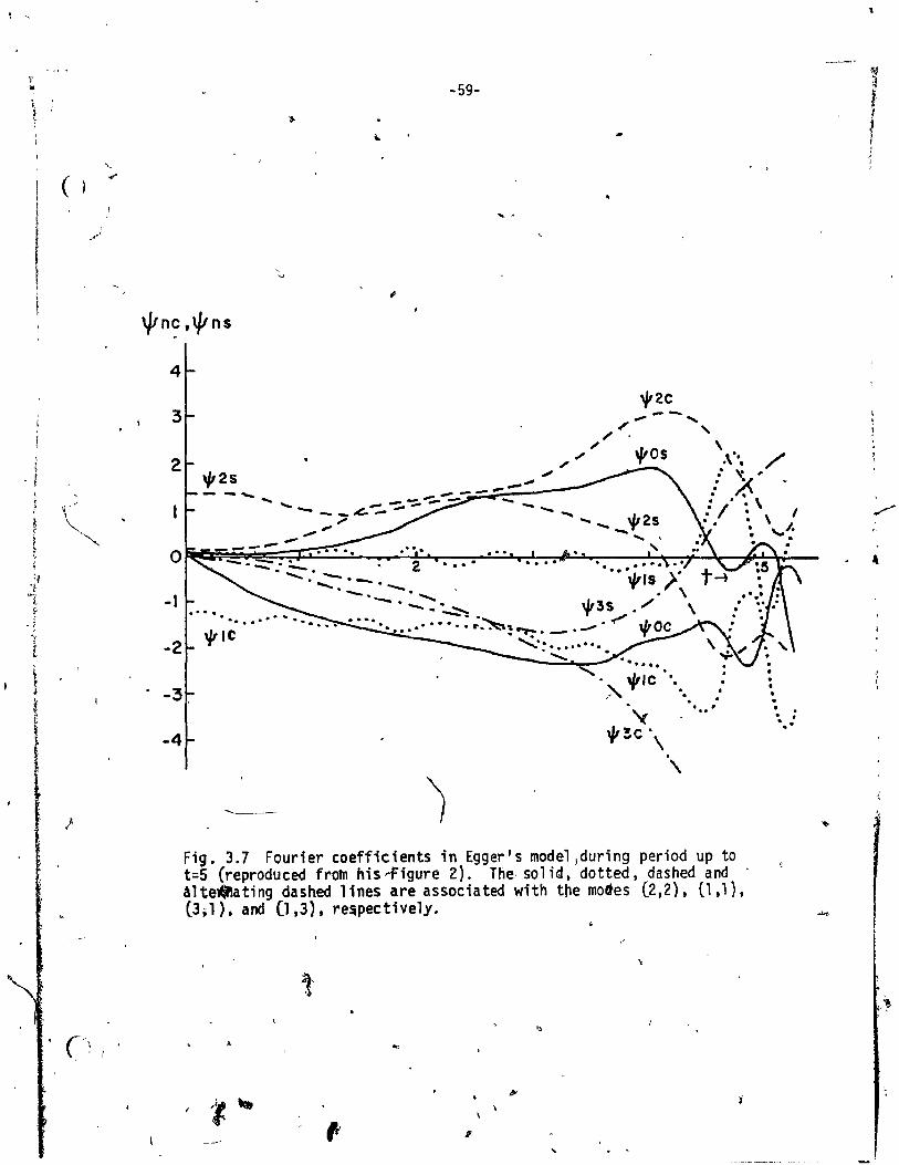
Fourier çoefficients are illustrated in Figure 3.7; we have defined the 9

,

~ ~ (2,2) and (1,3) modes ta be represented by kOl and k! , respective1y. '\

Evidently, the plock is created by the amplitude magnification of the (l,3),

(3,1) and (2,2) modes. The (1,1) mode generally~hows behaviour character-

istic of a sma 11 ampl itude free wave oscillating about a fixed forced

component with a frequency close to that predic.ted by linear theory. All • •

other waves exhibited negligib1e growth during the formation of the block.

The ~o~ coefficient initially underwent linear growth which began levelling

off at t-o.S , eventually reaching the level of-the forced waves at + .... , This initial linear growth turns out to be very near that predieted by

weakly nonlinear theory, which ;s hardly surprising. The other il1ustrated

modes also grew qu;te rapidly, in some cases (for instance \l'le) under­

go;n9 exponential growth. Once the block had broken down, irregu1ar be-

haviour developed in most of the modes. Our a;m in'th;s section will be

ta determlne to what extent weakly nonlinear theory.can help explain the

long time behaviour.

The ratio of t~e meridional perturbation velocity to the Doppler

shifted phase speed (commonly referred to as the interaction number) may

be evaluated for each of the two initially present forced modes, to deter-1

mine the amount of nonlinearity. involved 'in Egger 1 s tTI0de1. If this ratio , '

is O(lLor larger, the weakly nonlinear approach is no longer valid. In

his paper, Egger claimed that the interaction number approaches infinity

'w1th a stationary mode present, and hence that one must resort to numerical '\\

~j ..

-

/ 1

l, ,l,

,-, •

(

4

3

, l

. 1 2

t 1 "

-1

-59-

. ,

,.

~2e --- ..... tI' , ,. ,. \ " " ",os .,... /' .1. 2 s ."..: '\ .. T ~~ ~ - -"" ...,. --:.:;:-:.;-;::;:;:;.....--- . ';::' ...... ...... ..,. -::,..-=- - ....... : _. \

...... --_.,-:...... .................. :/ ~ 1 " . . . \ - ,. • ",,1. _...- ...... .,.. ~ .

." .. . .. ...... .::::::-.- :...... 2 . . . • . . . . .

'-.:~.-._ ""5)' t~ -0 0'-. • \

- • - _ :....::.- ~3S -. . . .. -.. . . .. -.~ . ~ ..... . ..... ~~.--- . .....,

----

, ........ -- . . '-. '

o ""e ", ... , -.. e' ~ ....

"'~C " '\

Fig. 3.7 Fourier coefficients in Egger's mode' }during period up to t::;5 (reproduced frotn his ..figure 2). Tfîe· so 1 id, dotted, dashed and ~lte.ating dashed Hnes are associated with the mottes (2,2), (l,l), (3.1). and (1 ,3). re~pectively.

,

. • • · • , . . '

, ,

~ ) , ,

" ~

" f f'

~

t

1

,-1

1 ,

,

1 ~

c

. ,.

-bU-

methods to proceed further. However, he based this conclusion 0D an , ,

incorrect definition of the interaction number which contained the

ordinary phase speed in the denominator. In terms of the previously

defined quantities. the two interaction numbers associated with the forced

waves can 8e shown to take the form

, n:; l, ~ . (3.47)

In the above. rand sare defined according to (3.44). • n n

Upon substitution

of the required values, we obtain

.i .,

Hence, it is evident that the forced wave ampl itude associated with the

(3.1) mode is large enough to prohiblt weakly nonlinear theory from being

used. This is due to the relatively large values of typical mid-latitude ,

forcing. and not because a stationàry wave is present in the model. Tc .. gain additional insight into the p'roblem, a numer;cal approach must be

considered. such as employed by Egger. We shall concentrate on the initial

growth stage to investigate the resonant fOrcing mechanism.

One can easily verity that no res~s. resonant quartets or

" resonant free-forced wave interactions exist in ,the truli\cated spectrum~

satisfying the approxJmate conditi~ns:

. ,

,

r

1 '. . J , ,

,', "

1 , _"

"

I--~--------~~~..----_ .. ~~--

-61-

or

1 {)ft" Wn 1 ,... 0 , -

respective1y. This leaves modal interactions as the major non1inear

resonance mechanism applicable to his model.

At this point r we define

(3.48.a)

(3.48.b)

, (3.48. c)

where the frequencies have been determined by the dispersion relationship

(2.12). The arbitrary sign convention for the wavenumbers has been chosen

to satisfy

(3.49)

We' represent the orders of the stationary and for.ced waves by '6 and E

respectfvely. The two forced waves will interact to produce a forcing for

the stationary wllte at o(e~l Free waves will be generated ,at higher

orders, when the forced waves have interacted tw;ce with each other or with ,

the stationary wave ta reproduce themsefves and must satisfy the initial

conditions at these orders. We then have the following ordering of terms:

stationary wave (AO)

forc~ waves ~Tl,T2)

stat10nary and forced wave interaction (AOT1,AOTZ)

1 1

\ ,

, .1

1

.

-62-

o (E"1) : forced waye interaction (T1T2); secular term for Ao

o(rt): secular term for AO (AOT/,AOT/) , production of higher order free waves .

For a balance of secular terms, we require

or

~= 1.

This result merely reflects the fact that the two forced waves cannot halt

the linearly resonànt growth through modal interaction~, since their inter-

action produces the resonant forcing. The stationary wave thus grows

linearly in time until the weakly nonlinear approach is no longer applicable.

This occurs quite early in the development, due to the large interaction

number associated with the forced (3,1) wave.

For small enough forcing, the weakly nonlinear approach wou1d have

undoubtedly have been val1d dur1ng the 1niti~1 growth stage, until the '~/O..J!.J

resonant mode had grown large enough ta induce unstable growth in the other

modes. This mechanism is somewhat related to the instability of a steady

p1anetary wave. as investigated by Lorentz 'X1972) and Gill (1974).

Another interesting case involves the presence of Jnitial free waves.

It is then possible that a weakly nonlinear approach could be used on the

long time sca1e. The tnave11ing ~odes might produce secular terms at ;

ote) which drive the stationary wave off its resonant frequency, as

explained in thè last section. Using the scaling arguments pre~ented

earlier, it can be shown that the t\avelling modes must be initially larger . than Ofe) for the weakly nonlinear apRroach to be val id. The 1 eading order

terms in the perturbation expansion would then involve one stationary mode

>

i 1

1 .

• -63-

and/or one or more travelling waves, which would not result in the

sustained blocking configuration obtained by Egger. Hence for a large

enough initial noise level, his resonance mechanism will not be efficient.

It should be noted that the exclusion of initial free waves is not a very

realistic cholce, since they are typically present in the atmosphere.

Egger's model demonstrates the importance of nonlinear interactions

in producing typically large resonant forcïng, as well as how the absence

of initial noi se can result in a 1 arge response"( in agreement with

Labitzke's (1978) results). In the rema ining chaptett we sha i'] deve10p

the general criteria required to produce resonant responses in more

realistic. non-uniform zonal flows. c.)

\ \ ~ ,~ .

, l" .;

.

1 . ,

" , ,

---~-~----~~--------------~--~ -- ---- --

. ,

\

t. Î

" ~

i' ,1

~ ~

(

•

CHAPTER 4 , RESONANCE IN SHEAR FLOWS WITH SMALl BACKGROUND NOISE

We have seen in the last two chapters that the initial noise 1eve1

plays a major role in the growth of planetary waves forced at resonance.

A large response was found to be possible provided that there was insuffi­

cient noise for the nonlinear effects to drive the stationary wave off its

resonant frequency. The wave then grows to a high leve1 at which the non­

linearities and/or damping mechanisms can finally check the resonant

growth. Having shown that this possibility exists for a uniform background,

flow. one might ask whether it holds for other, more rea1istic wind profiles.

In th;s chapter, we shall investigate the general conditions neeessary to

obtain resonant growth in shear flows, as first proposed by VJarn (private ~

communication). Both barotropic and baroel inic f10ws shall be eonsidered.

It shou1d be noted that the ensuing theory applies for the fully nonlinear 1

probl em. as well as for weakly nonl inear theory.

4.1 Barotropic flow

The inviscid, nonlinear, forced barotropic vorticity equation is

(~. + üty)..l)V.t}" +(e- ~)ll == Frx,y) (H' ~X cf y~ ~)(

t(I, 'V~!.L (4.1)

We look for separable solutions of the form

~ ,

~ ()(,Y,+) ==A(t> mo(x,y) (4.2)

where 10 satisfies the eigénvalue probl em

(4.3 )

, .

t

l j À j ~

a

\

(

't

-65-

associated with the eigenvalue (phase speed) c=o and a particular set of

specified boundary conditions. If mo is also of the f~rm such that

where G(fo}is an undetermined function, then the nonlinear terms vanish:

and using (4.2), (4.3), (4.4) and (4.5) in (4.1) yields

Hence. for a forcing

equation (4.6) reduces to

dt1 == n. dt

• 1Z= con st

In the absence of initial noise: -J

~ (t=o) = Q "0 . a:: const.

then

A(t) = a +nt

(4.5)

(4.6)

and the solution to (4.l) grows linearly with time. This resonance will

not occur in t~e presence of background noise. since solutions of the form

(4.2) will not be permitted.

'Thus, there are four requirements which need to be met: "

(i) (4.7.a)

\

, 1 t i

1 'l " -j

l "

, \ ;)

~~ t [.

, 1 1

'­,

\ ~;

t

(

t (" ~

{

p sn.

-66-

(i i)

(i i il

(i v)

F(x,y) ~ G (le)

i (10) = 0

\1:1~o = 6(~oL

(4.7.b)

(4.7.c)

(4.7.dl and

If one or more of these are only approximately satisfied. we may still

anticipate a reasonably large response. This has been shown in previous

chapters to be especially true for the initial noise restriction. Ta avoid j

having to specify the forcing and the boundary conditions. both (4.7.b)

and (4.7.c) shall be assumed to hold. In addition, we will assume that

the initial noise level is reasonably small enough that (4.7.a) is

approximately satisfied, and shall concentra te on the remaining require-

ment (4.7. d ).

The eigenvalue problem (4.3) may be rewritten in more convenient

form as

1- f vr:l ~o + [~ - Ü;q ] ~o l = 0 ~x l Û (y) J

where we have divided through by U(y), assuming it is non-zero. This

assumption 1s made throughout this chapter, to avoid deali~g with critical

layers. I,ntegrating with respect to x, using (4.7 .d) and dividing through

by 10+0 gives

+ B- Un = üey)

(4.8)

where 1f(y) is an arbitrary function arising from the partial integration.

The middle term is only a function of y while

consistency we must have 1r(y) :: 0

10 -= .10 (x, y) , 50 for "

q

\

- r

':­and

-67-

::1. = - (J' :. Co n ST.

l,

(4.9)

The negative sign is chosen in view of (4.7 .d). Substituting this result

into (4.7.b) indicates that the forcing must have the same spatial

structure as the stationary mode if resonance is to occur. Using the

above resu1ts in (4.8), we obtain

6:.Ü yy = cr:!. Uly)

or

with the associated general solution

qly) == R sirdcry-x) + a. cr:l.

(4.10)

(4.1l)

Any mean flow of this form will result in initial resonant growth of

a forced, stationary wave in the absence of initial noise. The constants

Rand :Xc!!n be determined by applying the associaied boundary conditions.

If p.= 0 then the zonal mean wind is constant, corresponding to the

profile used in the previous two chapters. There, we obtained resonant

responses in the absence of initial noise because our model included

resonant forcing, implying that al1 the conditions (4.7) were met. Thus,

the examples studied in the previous chapters are merely special cases of

the above general theory in the limit of van;shing initial noise. However,

both the uniform and the sinusoidal mean wind profiles do not reflect typieal

atmospheric conditions. lt therefore makes sense to proceed ta the more

realistic case involving baroelinic flow.

~ ;~

l '. "

" . , " j'

l

3

ff

"

\ /'

- ~~

(

'. , 1> 1

t " \

i ~ (,

-68-

4.2 Baroclinic flow

Using the theory presented in Charney (1973), the inviscid, nonlinear,

forced, baroc1inic potential vort;city equation ;s

(1. + û(y;z.)1. ) Q + ~ ~ dt 6X J y

.-J

f (x, y, 7.) (4.12)

where

Q= (4.13)

is the perturbation potentia1 vorticity and

(4.14)

is the mean potentia1 vorticity gradient. In the above, fo is the

pJanetary vorticity at the centre of the Beta plane, ~(Z) i5 the mea(~ atmospheric density and Jf(Z) i$ the Brunt-Va rssala frequency. As in the

-,

barotropic case, we shall assume that a stationary mode (~o) exists

having the same spatial structure as the forcing, and that the initial

noise level ;5 very small. For the nonlinear effects to vanish, we

require

(4.15)

such that

(4.16)

The stationary mode ïs as~med to satisfy the steady, unforced version of T ) •

(4.12) in the absence of non1 iné'ar effects:

') "- - ~" ___ ~ _____ r ..... _

, ~ , i

-

; t

i

i ,. f

i·

-69-

Ü(y2)~ + ~~ =0. ) ~X '6y ~x

Dividing through by Ü(y,Z)#O , using (4.15) and integrating with respect

to x yfe1ds

G (mo~z.) + ~o

(4.17)

where 1T'(y,Z) again represents an arbitrary function arising fram the

partial integration. Since the middle term is a function of y and Z only,

whirle ~o = Io(~)y,Z), we require

1f(y,Z) ::0

and

~= - (j (7.) •

Here, (J{z) is an arbitrary function of z, with the negative sign being

chosen in the spirit of (4.9). Using the above results, (4.17) reduces to

(4.18)

or using (4.14):

(4.19)

Due to the presence of the arbitrary function or(l), (4.19) can on1y

be studied once 0"(z1 is specified. In addition, suitable boundary

conditions and the mean atmospheric temperature profile must also be known.

On the other hand, (4.18) merely requires the knowledge of A values as a

function of latitude and height. These may be determined by assimi1ating

1 1

1 \ 1 , ,1

, "

r

-70-

zonally averaged global data during any particular time interval. If the

ratio of the mean potentlal vorticity gradient to the zonal mean wind

is indepenoent of y in a certain region of the y-z plane, then a resonant , '

planetary wave can exist t~ere in the presence of very sma11 initial noise.

Tn his investigation of vertica'lly propagating stationary waves,

Matsuno (1970) determined the variation of ~ with latitude and height in

the winter Northern Hemisphere. Althoùgh his study invo1ved spherical

geometry, the qualitative behaviour ;s not expected to change when the

simplifying Beta plane assumption is employed. His results are illustrated

in Figure 4.1. Averaged over the winter season. (4.18) is approximately

satisfied'north of the subtropics and up to about 10 km in height. The fact

that it does not seem to hold in .the equatorial region is of no concern,

since our quasi-geostrophic assumption is not applicable there either. Tt

therefore seems li~ely that the zonal mean wind in the winter Northern

Hemisphere permits the existence of resonant planetary waves in mid-latitude

tropospheric regions. One possible topic for future study might be to

determine whether similar regions exist on the average in the summer

Northern Hemisphere. In addition, past blocking situations could be ,

investigated in detail to determine whethel the conditions of resonant

forcing, lad of initial noise and !J.:F~(y) were satisfied. These concepts

may also be of use in practical meteorological applications. sinee they

can be used to forecast regions where blocking patterns might be expected

to oecur in the presence of very small initial noise.

,

f

C' ',' ,',

~,~, .; " "

t t i' , "

~

, l

.."

.'

~ l

~ ~

i f'

n

-71-

60

50

r ,......

~o ~ --) -..J

l-:t: <.!) ....... 30 L.LJ :::z:::

~o

!O

. . o 10 'lO 30 40 50

LATITUDE (0)--+ \

Fig. 4.1 The vadati,on of fJ. with he1ght and latitude, as detennined by r~atsuno (reproduced fram his Figure 3). ..

J 1

1 , 1 , 1

j

\ l l }

?

~I

l " 1

, ,

c

<,

-72-

. CHAPTE% 5

CONCLUSION

The main body of this work has dealt with the various types of nonlinear

interactions in a uniform, barotropic zonal flow. This model was chosen for

" its relative simpliclty; the resulting general principles are not expected

to differ in more realistic barocliniç flows. The weakly nonlinear limit

was cOnsidered to allow the use of an anàlytical approach. Using a straight­

forward asymptotic expansion in the spectral amplitude equations, a number

of nonlinear interactions were found to exist: resonant triads, resonant

quartets, modal interactions, forced-forced wave interactions and free-

forced wave interactions. The resonant triad co~ditions were hard to

satisfy, ~hile modal interactions were always present, but at a higher order.

Resonant quartets were not investigated in detail since they were similar in

many r.espects to resonant triads. Egger's (1978) model demonstrated how

(1) forced-forced wave interactions could create a resonant forcing and

(ii) the absence of initial noise might produce a significant response.

This resulted in a fully nonl inear flow, which mày accol:Jnt for his large­

scale blocking pattern. Unlike the other nonlinear processes, free-forced

wave interactions produced an amplifying travelling wave. This novel concept

may be significant in understanding the phenomenon of propagating upper air "

-troughs which amplify with time; it does,not, however. lead to the stationary

blocking pattern. of interest ta us.

In order to create lar~e-scal e block,1ng activity. our model required a

stationary planetary-scale wave which can in~era~resonantlY with the .

surface forcing. It was assumed that only one s~stationary mode existed. ,

, ! '

, 1 1

:-1\ , l . l '

!

'" -, ~ , , ~ '..., . ~t~ -7\

.~

, .v

r ,

, i

, '

e 44

") -.73-

1

,"

, -f

l"~

A natural closure of the s.ystem w~'s found to be associated with resonant , , . ,

triad interactions since a11 other waves~exchanged ene~gy through higher-• J

order mechanisms. 1Jsqng. fj~rtoft's (1953) B10cking Theorem, the cerltre

membe~ of the triad wàs determined ta be th~wave of intermediate ~en9th . ~

s~a 1 e. When the; r4esonant mode was the centra 1 member. the response to the , • ,\ T

forcing was bounded for al1 non-zero values of the normal ized (with respect' 1

"to t.he forcing) initial noise 1eve1, CL. ·~·For CL = 0, an unbounded res~onse

.. S pos.i b 1 e' under' cert:; n l-imi ti,~9 'i ni ti~+ condit i Jns, Whe~ the s ~ ;onory

~ve was a~ing member, an un1imited respqnse was found for CL < 1. Fo~' , .... , values of à ~ 1, an unbounded response was still possible, e?pe~;ally if the.

, initial energy in the r~sonant lJlode was, large enough. Whi1e these results l '9 1 ~ ......,

were obtained by solving a simpli~ied form of the forced rêsonant triad , ÂJ~" ~ ..

'equa~ions, it is nOlexpected that the overal1 concepts will différ in t~e

more general case.~· This m~ght be,confirm~ by obtaining numerical solutions

to the'general reso~a~t t~d amplitude eqUations.·' ".

, The ~tudy of m~daJ intera~tiàns fnvo1ving a 1inearlj reso~ant ~ode a1so

y1elded a finite response, whieh was inverse)y proportional bo the ratio of '1, ' ., \, \

101 the initial noise pa rame ter to the forcing. Hence in al1 types of nonlinear ~

interactions, ,.this nonnalized initial noise leve1 1S eViden,tly a crucial

factpr in determin1ng. the ~esonant response to an appli~d forciDg. Sinee , ".... " ! " ~

the re~oftant trià~ conditions are d1fficult to satisfy, the modal interaction • . mechan1sm 1s l1kely 'the most promi'nent n~nl inear atmospheric phenomenon.

I~ c~n, a1~o résult ~n an inf.injte r~sponse;~ forci ng ;~' doetuned by an

. r amount equal to the .. nonlinear frequency, shift. . \ ..

.. 0' .. J

~, -" ;. "

'. \ < ..

·f " --' t ,

1. ------ t. ,

11-~

• '1

,

...

~

1

'" '\

J 1

J ! !

.t ~

~

1

'1' }

'Z '1 v

"

j

" ' .

.

..

.'

't)

.

•

o

40

, r

-74-

..-" We 1ater derived the general conditions necessary to obtain resonant

responses tn barotropic and baroc1inic shear f10ws. Both required the

absence of initial noise (to be able ta neglect the nonlinear effects) and , the existence of a linearly resanant forcing. In addition, the zonal mean

wind "was restflcted to certain forms, ln the barotropic case, these

cons"isted of a sinusoidal and/or a constant component, while in the more

realistic baroclinic flow, the ratio of the mean potential vorticity

gradient to the zonal mean wind was required ta be independent of y. Since .

Matsuno's (1970) results indicate that this latter condition is 'fairly wel.1

satisfied in mid-latitude tropospheric regions in the winter Northern

~emisp~ere, this theory might account for the wave amplification observed

during tAis time period. Future studies involving these concepts could

prove very beneficial in forecasting blacking situations. { .

It is now possible"ta propose the.following expTanation for the 'creation

of large-scale blockif19 activity, based on tne above results. Ouring abnormal

a~sPheric' conditlons, the mean zonal wind (averaged throughout the whole

atmosPh~) ,becomes l~rge enough to render ~n ultra-long zonal harmonie

height wave stationary, If there 1s a distinct "lack of additional fr~e

waves and the background flow satisfies the previously stated requirements, ':

the nonline~~ effects.can be approximately negle&ted. A planetary-scale

re~an~ forcing will then cause the wave to grow tQ large amplitudes, at :~­

which t~me higher-order effects can finally suppress the growth. In winter, ,r;'

this,may lead to a sudden stratospheric warming, since the stratospheric

easterly jet core can trap the upwards-propagat1ng, resonant planetary waves. " -~

The conclusions ''Of thi s study may alsà be compared to the results . ' . J \'.

obtained by Charney and Devore (1979). Using an arbitrari1Y truncated

barotropic spectral model, they found the atmospheré to fluctuate between . , 1 ---'

~

t \

, 1

1-i j , ,

J

1 1

, 1

,-

",

5 b&iiiiiiiiii

~ 1

-

~ c' 1 1 .f

• \

\.

!

"

'LQ2

two stable regimes: a low index, zonal circulation and a high-index,

meridional flow. Thi~ was accomplished via a third, unstable mode,

Whil e the arbitrary truncation and the barotropic model do not conform

wi.th.atmospheric real ity, the result i s neverthel ess in agreement wi th

the obs~rved behaviour of the upper air flow., Our study has yielded

sorne relevant information on the transition from the zonal to the

meridiona1 circulation, at 1east in the weak.ly nonlinear '.imit, Future '

investigations could prove useful ,in analyzing the reverse procedure,

al thougi1_ it is apparent that weakly non1 inear theory would -no longer be \

applicatfle. More realistic zonal f10ws cou1d a1so be considered. The

su bS,equ en t r esu lts cou l d go a long way towa rd s à bet ter und er s tâ'nd i "g

and fm-ecasting of t-he dyn,amical ,atmospheric circulation.

.' ,.

/

1 i -

" -, .

...

r

~ 1 " ' ,

~

.1'

~/' ~

! " .' " ~

j ]"

~ t ~

, ,

coq p

-76-

BIBLIOGRAPHY

\

Abramowitz, M., and I.A. Stegun, 1964: flandoook of mathematici!.l functions with formulas, graphs and mathematlcal tables. U.S. Dept. of Commerce, Nat. Bur'. ?tnds., 1046 pp.

Armstrong, I.A., N. Bloembergen, J. Ducuin~, and P.S. Pershan, 1962: Light waves in a non-linear dielectric. Phys. Rev., 127,1918-1939 . .

Benney, D.J., 1962: Non-1inear gravit y wave interactioos. J. Fluid. Mech., '14, 577-584 ..

t

Benney, D.J., 1979: Instabilities associated with forced non1inear waves. Stud. Appl. Math., 60,., 27-41.

Bretherton, F.P., 1964: Ilesonant interactions between waves" The case of discrete oscillatiBtts .. ~. Fluid Meeh., 20, 457-479.

Charney, J.G., 1973: Planetary f1uidOdynamics. In Dynamic Meteoro1ogy, edited by P. Morel. D. Reide1 Pub1ishing Co:, Dordrecht-Hol1and/ Boston - U.S.A., pp. 97-352.

Charney, J.G., and J.G. Dev~re, 1979: Multiple f1ow~quilibria in the atmosphere and blocking. To be published.

~ Charney, J.G., and P.G. Drazin, 1961: Propagation of p1anetar;-scale \. disturbances from the lower i~to the uppe~ atmosphere. J. Geophys. Res., 66,83-109.

Clark, J.H.E., 1974: Atmospheric response \{> the quasi-resonant growth of forced p1anetary waves. J. Met. Soc. Japan~ 52, 143-195.

Davidson. R.C •• 1972: Methods in non-1inea-r ,p/lasma theory. Academie Press, New York, 356 pp.

Dickinson. R.E.. 1968: P1anetary Rossby waves propagating vertically through weak wester1y wind guides. J. Atmos. ~ci .• 25, ~84-1002. ,

Dickinson, R.E., 1968: On the exact ~ approximate linear theory of vertiea11y propagating planetary Rossbytwaves forced at a spherital

, lo~er boundarY. Mon. "ea. Rev •• 96, 405-415. . . ~. ,

Domaracld, A., and A.Z. Loeseh, 1977:, "on~1inear o~interactiolls among equatorial waves. J. t~tm~. SoC~t. 34, 486 .. 4~8. , " .

Ouffy, D.G., 1974: Resonant interactfons of inertia1 gravit y and Rossby ': waves. J. Atmos. Sei., 28, 1218-1231. '

.,'

JI..

...

"

"

i

1

~,

c

,. \

..

\ -77-

Egger1 J., 1978: Dynamics of blocking highs. J. Atmos. Sei,; 35, 1788-1801 .

.fj~rtoft, Ragnar, 1953: On the changes in the spectral distribut·ion of ~inetic energy for two-dimensional, non-divergent f10w. Te11us, 5, 225-230.

Gill, A.E., 1974: The stabil ity of p1anetary waves on an infinite Beta plane. Geophys. F1uid Dyn., 6,~-47,. -

Hasse1m,ann, K., 1967: A criterion for non1inear wave instability. J. Fluid Mech., 30, 737-739.

Hirota, I., 1968: On the dynamics of long and ultra-long waves in a baroc1inic zonal current. J. Met. Soc. Japan, 46, 234-249.

Holton: J.R., 1975: The dynamica1 meteoro1ogy of the stra~osphere and mesospher:;e. Lancas~ Press, Lancaster, 216 (~~ _____ /

. ---' Holton, J.R., 1~7&: A semi-spectral mmerical mode'r for wave-mean flow intera~tio~ in the stratosphere: Applicatîon ta sud den strataspheric warmings. J. Atmos. SeL, 33.1639-1649.

-Holton, J.R., and R.S. lindzen. 1972: An updated theory for the quasi-

bienni'al oscillation of the tropical stratosphere. J. Atmos. Sci., 29, )076-'1080. 1

Kao, S.K., and H.N. Lee, 1977: The non-linear interact'Ïons and maintenance of the 1arge-sca1e.moving waves in the atmosphere. J. Atmos. ~ci.~ 34, 471-485. i

.' ,

Labitzke, K., 1978: On the different behaviour o'i-the zl.bnal hannonic height waves l and 2 during the winters 1970/71 and 1971/72. Mon. Wea. Rev., 106, 170Ml713. ' ~

Longuet-Higgins, M.S., and D.M. Phtl1ips, 1962: Phase velocity effects in tertiary wave interactions. J. Fluid Mech.·, 12, 333-:33-6.

~onguet-Higgins, M. S., and A.E. Gill, 1967:- Resonant interactions between planetary waves. ,Proe. Roy. Soc. London, A299, 120-140.

Lorentz, E. N., 1960: traXimum simplification of the dynamic equations. Tellus. 12, 243 .. ~. . . -Lorentz, LN." 1972: Barotropic instability·of Rossby wave motion. J. Atmos. Sei., 29, 256-2.64.

,

Matsun~ T" 1970: Vertical propagation of stationàry planetary waves ,in' thewinter northern hemisphere. J. Atmos. Sct., 27, 871.:.aa3.

, ,

t

.. '

-78-

Matsuno, T., 1971: A dynamica1 mode1 of the sudden stratospher;c warming. J. Atmos. ScL, 28, 1479-1494.

Nayfeh, A.H., 1973: 425 pp.

Perturbation methods. 'Ji

John Wiley and Sons, New York, ,

Phillips, O.M .• ~n: O~the dynamics of unsteady gravit y waves of finite amp 1 itude:~ J. F1 uid Meeh., 9, 193-217. Il

Ritchie, C.H .• 1978: Numerica1 simulàtion of eritiea1 layer evo1ution. M'.Se. thesis, McGil1 University. Montreal, Quebec.

Tsay, C.Y., and S.K. Kao, 1978: Linear and non1inear contributions to the growth and decay of the 1 arge-scale atmospheric waves and jet stream. Tell us. 30, 1-14.

Tung, K.K., 1977: Stationaryatmospheric long waves and the phenomena of , blocking and sudden warm;ng. Ph.D. thesis, Harvard University,

Cambridge, Massachusetts. -Vickroy. G .• and J.A. DuttCW. 1979: Bifurcation and catastrophe in a

simple. foreed, dissipative quasi-geostrophic f1ow. J. Atmos. Sei.. 1 36, 42-52.

•

)

t " "

l'

1 , ;

1 î

~ i

\

,

l'

".

J ,

~"' l

.-',1 ~ '\1 ~

" ~; !