a study of polluted eco-system of industrial areas …
TRANSCRIPT
A STUDY OF POLLUTED ECO-SYSTEM OF INDUSTRIAL
AREAS CAUSED BY THE INDUSTRIAL EFFLUENTS
A thesis submitted
to
Bahauddin Zakariya University
in fulfillment of the requirement for the degree of
DOCTOR OF PHILOSOPHY
in
Chemistry
By
SYED NOOR-ULLAH HUSAINI
Department of Chemistry, Bahauddin Zakariya University,
Multan, Pakistan
2008

II
IN THE NAME OF
ALLAH
WHO IS THE MOST GRACIOUS AND MERCIFUL

III
This dissertation is dedicated to my loving father
SYED MINALLAH HUSAINI (Late)
Who was a beacon of true Muslim, integrity and honest

IV
Declaration of originality
I hereby declare that the research work and the intellectual contents of this thesis
are the outcome/ fruit/ results of my own worth. This thesis has neither been previously
published in any form nor does it contain any verbatim of the published resources which
could be treated as infringement of the international copyright law.
I also declare that I do understand the terms “copyright” and “plagiarism” and that
in case of any copyright violation and plagiarism found in this work, I would be fully
responsible for the consequences of any such violation.
Most of the work of this thesis has been published in my different international/
national publications. The lists of such research publications and presentations are also
endorsed here.
Signature:______________________ (Syed Noor-ullah Husaini)

V
Department of Chemistry Bahauddin Zakariya University,
Multan, Pakistan
Certificate This is to certify that we have read this thesis entitled “A Study of
Polluted Eco-System of Industrial Areas Caused by the Industrial
Effluents” carried out by Syed Noorullah Husaini and that in our opinion,
it is fully adequate in scope and quality for the degree of Ph.D. in Chemistry.
The work contained in this thesis has been carried out under our supervision
and is approved for submission in fulfillment of the requirement for the
degree of Doctor of Philosophy in Chemistry.
Approved by: Signature:_________________ (Supervisor) DR. JAMSHED HUSSAIN ZAIDI Chief Scientist Director Science PINSTECH, P.O. Nilore, Islamabad, Pakistan.
Approved by: Signature:_________________ (Supervisor) PROF. DR. MUHAMMAD ARIF Department of Chemistry, Bahauddin Zakariya University, Multan, Pakistan.
Approved by External Supervisor:
Signature:_________________
VI
Acknowledgement In the name of ALLAH, the most merciful and his Holy Prophet MUHAMMAD
(Sallalaho Allihi wa Aalahi wa Sallam), who is forever a source of guidance and
knowledge for human being.
I feel highly privileged to express my sincere and deep gratitude to my respected
supervisor Dr. Muhammad Arif, Professor of Chemistry, Department of Chemistry, Baha-
ud-Din Zakariya University, Multan, for his supervision, best cooperation and
encouragement through out the course of this research.
I gratefully acknowledge Dr. Syed Jamshed Hussain Zaidi, Chief Scientist and
Director Science PINSTECH, my honorable co-supervisor, for his enthusiastic guidance,
keen interest and persistent support. He has always been a source of enlightenment,
knowledge and cooperation for me in all fields of life. I feel a real honour to complete my
Ph. D. under his kind supervision.
I also wish to express my gratitude and admiration to Dr. M. Arif, Dr. Matiullah,
Dr. Shahida Waheed, Dr. Ismat Fatima, Dr. Shahid Pervez and Dr. M. Aslam for their
help, constructive criticism and valuable suggestions. My special thanks to Dr. Shoaib
Ahmad, Member Physical Sciences and Dr. J.I. Akhtar, Head Physics Division for their
full cooperation and gracious attitude to complete this research work in time.
I realize that the fulfillment of Ph.D. task is a collective effort, which involves the
guidance, cooperation and help of my well wishers. I would like to pay greatest thanks to
my in-laws, especially Mr. Shahid Munir Qureshi, Syed Badar-ul-Hassan Chishti and Dr.
Saeed-ul-Hassan Chishti for their cooperation in the collection of samples and valuable
contribution for the completion of the manuscript. I appreciate Syed Junaid Akhtar for his
cooperation and help in computer programming. Heartiest thanks are extended to my all
colleagues (officers and staff members) especially Dr. I.E. Qureshi, Dr. E.U. Khan, Dr.
M.I. Shahzad, Dr. S.A. Mujahid, Mr. M. Akram, Dr. S. Karim, Mrs. F. Malik, Dr. M.
Daud, Mr. A.K. Rana and Mr. Amjad Mehmood for their help and cooperation.
It is a fact that without the cooperation of my family, it was not possible for me to
get the Ph.D. degree. My special thanks are for my mother, wife, children, sisters and
brothers for their continuous help, endless cooperation, moral support, encouragement,
patience and sacrifice in all respects.

VII
Abstract
The adverse effects of industrial pollution are becoming a challenge for
scientists and environmentalists around the globe. The management of the pollution is
imperative to improve the human health, economy, aquatic life and to protect from further
deterioration of the environment. The leading intend of the present work was to evaluate
trace elemental contaminations in agricultural soil, crops and vegetables being irrigated
with industrial effluents and their treatment to reduce the pollution. This research will be
beneficial to decrease the industrial pollution by the immobilization of the toxic
constituents in the effluents and will provide database pertaining to the concentration of
metals in the industrial effluents and their accumulation in soil, crops and vegetables. The
data will assist to identify the trends, nature, and sources of pollution and will aid in the
formulation of legislation related to the controlled release of industrial effluents into the
environment. Moreover, present data for nutrition can be useful for nutritionists and food
technologists for the formulation of diet menu for the inhabitants of the respective regions
with adequacy/ safety viewpoint for balance intake of essential and toxic trace elements.
For this research, more than 500 samples of vegetables (brinjal, baffle gourd,
ridged gourd, tomato, pumpkin, bitter gourd, cabbage, mustard, spinach, potato, turnip,
radish & carrot), crops (millet, maize, rice & wheat), effluents (ceramics, pulp/paper &
textile/yarn industries) and soils (top & sub-surfaces) have been collected from the
vicinity of industrial zones of Faisalabad and Gujranwala areas. Each species of vegetable
and crop plants was separated into its fruits (edible portion), flowers, leaves, stems and
roots to evaluate the bio-distribution of trace elements, in each portion. Neutron
Activation Analysis (NAA) and Atomic Absorption Spectroscopic (AAS) techniques
have been utilized to analyze the selected samples for the quantitative determination of
more than 36 trace and toxic elements. Accuracy and precision have been ensured by
comparing with five different certified reference materials (CRMs) and by making
replicate measurements for each sample. Moreover, the Z-score method was also applied
to assess the discrepancy between the measured and the certified values.
Ultra-filtration membrane therapy (UFMT), which is a separation technique,
was used for the reduction of toxic level in industrial effluents. Various runs have been
conducted on samples of the effluents by using a lab-scale UFMT unit, which was fitted

VIII
with a Polyethylene tere phthalate (PETP) membrane. This filtration technique is very
effective, reliable and economical for the quantitative separation of suspended particles
from the effluents. The effects of temperature and pressure on flow rates of the effluents
have been investigated. The parameters such as flux, temperature, applied pressure,
filtration velocity, density, concentration of the effluents and their relationships have been
illustrated. Spectro-photometric analyses prove the effectiveness of UFMT system in
removing dissolved coloured species and chromate ions also. The pollution parameters
such as colour/ dyes, biochemical oxygen demand (BOD), total suspended solids (TSS),
total dissolved solids (TDS), turbidity, oil/ grease/ fat etc., have been reduced
quantitatively up to 96% in the post filtration effluents. Moreover, in the absence of other
electrolytes, the chromate removal up to 98.9% from effluents has also been achieved.
Arsenic, chromium and iron metals have also been successfully removed from
the industrial effluents, on laboratory scale, by using husk of sweet peanut. In this regard,
optimize experimental parameters have been established for smooth/reliable performance.
The analytical results for the concentrations of 36 minor, major, rare earth and
toxic elements in each sample of vegetables, cereal, soil and effluents are presented in
tables 6.1 to 6.12. Moreover, the evaluated concentrations of some selected trace elements
have been presented in figures 7.4 7.41 for their comparison patterns with each other.
The results of physico-chemical analysis and trace elemental concentrations
showed that all untreated effluents were un-fit for irrigation purposes due to the higher
values of metals as compared to the NEQS values. Effluents vary in quality for textile,
pulp, and ceramics industries and are specific for each industry. The effluent
contamination has been decreased in the following pattern.
Textile/ Yarn Pulp/ Paper Ceramics
Faisalabad industrial area was divided into four zones (i.e. F-1, F-2, F-3 & F-4).
Zone F-1 represents the area of Industrial Estate, F-2 represents the area of Ghulam
Muhammad abad, F-3 represents the area of Peoples Colony and F-4 represents the area
of Sitara Colony. According to the high concentration of the elements, the intensity of
toxicity in the specified soils of Faisalabad is decreased in the following order.
F-1 F-2 F-3 F-4

IX
Similarly, Gujranwala industrial area was divided into four zones (i.e. G-1, G-2,
G-3 & G-4). Zone G-1 represents the area of Dhula, G -2 represents the area of Garjakh,
G -3 represents the area of Small Industrial Estate and G-4 represents the area of
Muhammad Nagar. Moreover, due to the high concentration values of concerned
elements, the intensity of the toxicity in the specified soils of Gujranwala shows the
following decreasing sequence.
G-4 G-3 G-2 G-1
Leaching tendency of some selected trace elements was observed for Faisalabad
and Gujranwala soils. The elements (i.e. Ba, Cr, As, Na, Cl, K, Br & Mg) move from
topsoil (St) to sub-soil (Ss) very easily as compared to other elements (i.e. Mn, Sb, Sc, Co,
Se, Fe & Zn) due to high leaching tendency. The same behaviour was observed in both
soils of Faisalabad and Gujranwala. Therefore, the quantities of the elements (i.e Ba, Cr,
As, Na, Cl, K, Br & Mg) are higher in sub-soils as compared to the topsoil. This behavior
was also confirmed by the evidence of observed high electrical conductivity (EC) values
(5.6-4.3 S cm-1) at sub-soil as compared to topsoil (4.1-3.1 S cm-1) values.
According to the concentrations of the trace elements, the industrial (Gujranwala
& Faisalabad) and non-industrial (Rawalpindi & Islamabad) national soils are arranged in
the following descending series.
Gujranwala > Faisalabad > Rawalpindi > Islamabad
A comparison was made among the national soils (i.e. Faisalabad &
Gujranwala) and international soils (i.e. Norway & India). All soils samples were
analyzed using NAA technique. According to the high concentrations of the trace
elements, generally all zones are arranged in the following sequence.
Gujranwala > Faisalabad > Norway > India
Vegetables are staple part of food and are widely consumed in all over the
world. The determination of metal contents in vegetables is significant from the
viewpoint of crop-yield technology, food nutrition and health impacts. The differences for
the accumulation of mineral/ metal contents in the edible portions of vegetables depend
upon the soil compositions and the rate of uptake of minerals/ metals by each plant.
Results showed that different vegetables had different abilities to take up heavy metals.

X
However, the general trend shows that the maximum concentration of the trace elements
is accumulated in roots while their least concentration is found in fruits i.e. edible part of
the vegetables and are arranged in the following decrasing sequence.
Roots Stems Leave Fruits (Edible portion of vegetables/ crops)
All over the world, about 70% of human diet consists of cereals and legumes. In
case of edible portion of cereals the toxic activity decreases in the following sequence,
which indicates that wheat crop is the least affected by the industrial effluents as
compared to other cereal crops.
Millet Maize Rice Wheat
It was observed that the concentrations of all elements are high in the wheat of
Faisalabad and low in the wheat of Kashmir. The order of toxicity decreases as following:
Faisalabad Gujranwala Islamabad Kashmir
The concentrations for majority of elements are high in the rice of Faisalabad
and low in Kashmir. The order of toxicity decreases in the following sequence.
Faisalabad Islamabad Gujranwala Kashmir
Similarly, the concentrations for majority of elements are high in the vegetables
of Faisalabad and low in Islamabad. The order of toxicity decreases as under:
Faisalabad Gujranwala Kashmir Islamabad
Regular monitoring for further assessment as to ascertain the quality of the
foodstuffs and the origin of trace metal distribution is a pre-requisite. In order to obtain
consolidate achievements numerous analyses of various species are required where
seasonal and regional variations need to be studied in detail.

XI
LIST OF CONTENTS
Sr. # Captions Page #
Bismillah II Dedication III Declaration IV Certificate V Acknowledgement VI Abstract VII List of Tables XVI List of Figures XIX List of Abbreviations XXI
Chapter-1 1. INTRODUCTION 1 1.1. Eco-system 2 1.2. Pollution 3 1.2.1. Air Pollution 4 1.2.2. Water Pollution 4 1.2.3. Land Pollution 5 1.2.4. Noise Pollution 5 1.2.5. Radioactive Pollution 5 1.2.6. Thermal Pollution 6 1.2.7. Industrial Pollution 6 1.2.7.1. Type of Industrial Pollutants 7 1.2.7.2. Environmental Impacts of Industrial Effluents 7 1.2.8. National Environmental Quality Standards (NEQS) 9 1.3. Monitoring Techniques for the qualitative and quantitative
determination of Industrial Pollution 11
1.3.1. Conventional Analytical Techniques 12 1.3.2. Nuclear Analytical Techniques 14 1.4. Neutron Activation Analysis (NAA) 15 1.4.1. Sensitivity and Detection Limits of NAA 17 1.4.2. Industrial application of NAA 19 1.4.3. Advantages of NAA 20 1.4.4. Limitations of NAA 20 1.5. Atomic Absorption Spectroscopy (AAS) 21 1.5.1. Theoretical Aspects of AAS 21

XII
1.5.2. Advantages of AAS 22 1.5.3. Limitations of AAS 22 1.5.4. Sensitivity and Detection Limits of AAS technique 23
Chapter-2 2. LITERATURE REVIEW 24 2.1. Industrial effluents 24 2.2. Agricultural soils 25 2.3. Vegetables 26 2.4. Crops 28
Chapter-3 3. AIMS AND SCOPE 29 3.1. Motivation 29 3.2. Research Objectives 30 3.3. Work Plan 30 3.4. Working Strategy 31 3.4.1. Sampling and Sample Preparation 31 3.4.2. Analysis 32 3.4.3. Data Processing 32 3.4.4. Decontamination Procedures 32
Chapter-4 4. EXPERIMENTAL WORK 33 4.1. Sampling 33 4.1.1. Sample collection 33 4.1.2. Samples preservation 37 4.1.3. Sample preparation 38 4.1.4. Sample identification 39 4.2. Reference materials for NAA 42 4.2.1. Preparation of secondary standards 45 4.3. Irradiation facilities 46 4.3.1. Pakistan Research Reactor –1 (PARR-1) 46 4.3.2. Pakistan Research Reactor –II (PARR-II) 48 4.4. Irradiation technique 49 4.4.1. Container/ rabbit for irradiation 50 4.4.2. Calculations for the measurement of radio-activity 50 4.4.3. Protocol for sample irradiation 52 4.5. Gamma - Spectrometric Instrumentation 53
4.5.1. Description of Instruments for NAA 55 4.5.2. Calibration of the detectors 55

XIII
4.5.3. Essential parameters for the Gamma spectrometry 55 4.5.4. Gamma scanning of the radio nuclides 56 4.6. Statistical Calculations 58 4.6.1. Correction with back ground counts 58 4.6.2. Decay Factor 59 4.6.3. Concentration of elements 59 4.7. Preparation of solutions for AAS 60 4.7.1. Stock solutions 60 4.7.2. Standard blank solution 61 4.7.3. Standard solutions 61 4.7.4. Solutions of geological and effluent samples 61 4.7.5. Blank solution for geological and effluent samples 62 4.7.6. Solutions of crop and vegetable samples 62 4.7.7. Blank solution for crop and vegetable samples 62 4.8. Analysis of samples through AAS 63 4.8.1. Atomic Absorption Spectrometric Instrumentation 64 4.8.2. Analytical parameters for AAS analysis 65 4.8.3. Instrumental operating conditions and specifications 65 4.9. Sources of errors 66
Chapter-5 5. RESULTS (Evaluation of trace elements) 67 5.1. Validation of methodology for NAA technique 67 5.2. Validation of methodology for AAS technique 69 5.3. Trace elemental contents in the Effluents 70 5.4. Trace elemental contents in the Soils 77 5.5. Trace elemental contents in the Crops 82 5.6. Trace elemental contents in the Vegetables 86
Chapter-6 6. TREATMENT OF INDUSTRIAL EFFLUENTS 90 6.1. Introduction 90 6.2. Objectives of effluent treatment 90 6.3. Utilization of fresh water in the industries 91 6.4. Industrial wastewater pollution 91 6.5. Need for the pollution control in the industry 92 6.6. Technologies for the treatment of industrial effluents 92 6.7. Existing processes for the industrial effluent treatment 93 6.8. Industrial effluent treatment by Ion Track Filters 94 6.8.1. Membrane filtration and its advantages 95 6.8.2. Membrane 95

XIV
6.8.3. Configuration of Ultra-filtration plant 97 6.8.4. Membrane fouling 99 6.8.5. Membrane cleaning 99 6.8.6. Membrane performance 100 6.8.6.1. Effect of Effluent’s Concentration on Flux 100 6.8.6.2. Effect of Effluent’s Concentration on Filtration Velocity 101 6.8.6.3. Effect of Temperature on Flux 101 6.8.6.4. Effect of Temperature on Filtration Velocity 102 6.8.6.5. Effect of Time on Electrical Conductivity 103 6.8.6.6. Effect of Time on Filtration Velocity 103 6.8.6.7. Effect of Density on the Filtration Velocity 104 6.8.6.8. Effect of Pressure on the Filtration Velocity 105 6.8.6.9. Effect of Flux 106 6.9. Removal of Pollutants 106 6.9.1. Reduction of BOD 108 6.9.2. Separation of TSS 109 6.9.3. Elimination of oil and grease 109 6.9.4. Removal of turbidity 109 6.9.5. Retardation of TDS 110 6.9.6. Extraction of dyes 110 6.9.7. Removal of chromium 111 6.10. Sweet peanut husk, a potential scavenger 112 6.10.1. Low cost materials 112 6.10.2. Sweet peanut husk 112 6.10.3. Purification/ preparation of peanut husk’s material 113 6.10.4. Solutions preparation 113 6.10.4.1. Buffer solutions 114 6.10.4.2. Stock/ Standard solutions of Acids 114 6.10.4.3. Standard solution of Arsenic 114 6.10.4.4. Standard solution of Chromium 115 6.10.4.5. Standard solution of Iron 115 6.10.5. Physico-chemical parameters to optimize the conditions 115 6.10.6. Adsorption process (Experimental) 115 6.10.7. Analysis of Industrial Effluents 117 6.10.7.1. Chromium (Cr) 117 6.10.7.2. Arsenic (As) 118 6.10.7.3. Iron (Fe) 118 6.10.8. Effect of pH 119 6.10.9. Effect of acid concentrations 120 6.10.10 % Removal of concerned metals 122

XV
Chapter-7 7. DISCUSSION 123 7.1. Quality assurance for the Results 124 7.2. Solutions for the interferences in Gamma peaks 126 7.3. Industrial Effluents 128 7.3.1. Physico-Chemical Analysis of Effluents 128 7.3.2. Effluents of Textile/ Yarn Industry 130 7.3.3. Effluents of Pulp/ Paper Industry 131 7.3.4. Effluents of Ceramics Industry 132 7.3.5. A comparison among the effluents of textile, pulp and ceramics
industries 133
7.4. Faisalabad & Gujranwala Soil 135 7.5. Faisalabad and Gujranwala Crops 142 7.5.1. Faisalabad & Gujranwala Wheat 143 7.5.2. Faisalabad & Gujranwala Rice 148 7.5.3. Faisalabad & Gujranwala Maize 152 7.5.4. Faisalabad & Gujranwala Millet 156 7.5.5. A comparison among cereals (grains) for the evaluation of toxic
levels 160
7.6. Faisalabad & Gujranwala Vegetables 162 7.6.1. Faisalabad & Gujranwala Summer Vegetables 163 7.6.2. Faisalabad & Gujranwala Winter Vegetables 167 7.6.3. Faisalabad & Gujranwala under-ground Vegetables 169 7.7. Comparison of crops, vegetables and soils with literature
reference values
172
Chapter-8 8. CONCLUSIONS AND RECOMMENDATIONS 181 8.1. Conclusions 181 8.2. Recommendations 183 References 184 List of Publications Papers Presentation in Conferences

XVI
LIST OF TABLES
Table 1.1 Industrial media with possible pollutants 7 Table 1.2 Adverse environmental impacts of industrial effluents 8 Table 1.3 National Environmental Quality Standards (NEQS, 1997) for
Municipal liquids and Industrial effluents 10
Table 1.4 Detection limits and relative errors for different analytical techniques
12
Table 1.5 Calculated detection limits for neutron activation analysis 18 Table 1.6 Sensitivity (g/g) of NAA technique for metals 19
Table 1.7 Sensitivity (g/g) & Detection Limits (g/g) of AAS techniques 23
Table 4.1 List of the crops / vegetables cultivated within the vicinity of industrially polluted areas of Faisalabad and Gujranwala cities
36
Table 4.2 Codes for samples of the crops and vegetables 40 Table 4.3 Codes for samples of the soil 41 Table 4.4 Codes for samples of industrial effluents 42 Table 4.5 Description of geological and biological reference materials/
standards 43
Table 4.6 IAEA Reference sheets (1999 & 2000) for cited values of Biological (Lichen, CL & WP) and Geological (SL-1 & S-7) standards
44
Table 4.7 Specifications of Pakistan Research Reactor-1 (PARR-1) 47 Table 4.8 Specifications of Pakistan Research Reactor-II (PARR-II) 48 Table 4.9 Nuclear data, essential to calculate the activity of the elements for
irradiation 51
Table 4.10 Operating conditions for the Gamma spectrometric analysis 56 Table 4.11 Nuclear data for intermediate term irradiation conditions (05 to 10
min) of crops, vegetables and soil samples at PARR-1 56
Table 4.12 Nuclear data for intermediate term irradiation conditions (25 to 35 min) of crops, vegetables and soil samples at PARR-1
57
Table 4.13 Nuclear data of long-term irradiation conditions (300 min) for crops, vegetables and soil samples at PARR-1
57
Table 4.14 Nuclear data of short-term irradiation conditions (02 minute) for crops, vegetables and soil samples at PARR-2
58
Table 4.15 Analytical parameters for AAS analysis 65 Table 4.16 Instrumental operating conditions and specifications for AAS 65

XVII
Table 5.1 Comparison of the trace elemental concentrations (g/g) for reference values of biological (Lichen, Citrus Leaves & Whey Powder) and geological (SL-1 & S-7) Standard Reference Materials (SRMs) with present work analyzed through NAA technique
68
Table 5.2 Comparison of the trace elemental concentrations (g/g) for reference values of IAEA Standard Reference Materials (SRMs) with present work analyzed through AAS technique
69
Table 5.3.a
Concentrations (g/g) of trace elements in the effluents of textile/ yarn industry
71
Table 5.3.b
Concentrations (g/g) of trace elements in the effluents of Pulp/ paper/ board industry
72
Table 5.3.c
Concentrations (g/g) of trace elements in the effluents of Ceramics industry
73
Table 5.4.a
Physical analysis of Textile/ Yarn industrial effluents, collected from industries of Faisalabad and Gujranwala
74
Table 5.4.b
Physical analysis of Pulp/ Paper industrial effluents, collected from industries of Faisalabad and Gujranwala
75
Table 5.4.c
Physical analysis of Ceramics industrial effluents, collected from industry of Gujranwala
76
Table 5.5 Concentrations (g/g) of trace elements in the soils of Gujranwala’s industrial areas
78
Table 5.6 Concentrations (g/g) of trace elements in the soils of Faisalabad’s industrial areas
79
Table 5.7 Concentrations (g/g) of trace elements in the agriculture soils of Islamabad and Rawalpindi Non-industrial zones
80
Table 5.8 A comparison among the concentrations (g/g) of trace elements in the international and national soils
81
Table 5.9.a
Concentrations (g/g) of trace elements in Faisalabad’s crops (Fruits)
82
Table 5.9.b
Concentrations (g/g) of trace elements in Gujranwala’s crops (Fruits)
83
Table 5.10.a
Concentrations (g/g) of trace elements in Faisalabad’s crops (Leaves)
84
Table 5.10.b
Concentrations (g/g) of trace elements in Gujranwala’s crops (Leaves)
85
Table 5.11.a
Concentrations (g/g) of trace elements in Faisalabad’s summer vegetables (Edible portion)
86
Table 5.11.b
Concentrations (g/g) of trace elements in Faisalabad’s winter & underground vegetables (Edible portion)
87

XVIII
Table 5.12.a
Concentrations (g/g) of trace elements in Gujranwala’s summer vegetables (Edible portion)
88
Table 5.12.b
Concentrations (g/g) of trace elements in Gujranwala’s winter & underground vegetables (Edible portion)
89
Table 6.1 Commercial ultra-filtration membranes 96 Table 6.2 Optimized operating parameters of UFMT unit 98 Table 6.3 Pre and post filtration values, with standard deviations, of the
pollutants along with their recommended values for the effluents of textile/ yarn industry
107
Table 6.4 The contamination levels with standard deviations, before and after the purification, for the effluents of pulp/paper/ board industry along with their recommended values
108
Table 6.5 Preparation of buffer solutions (pH 1-12) 114
Table 7.1 A comparison of physico-chemical parameters among the effluents of textile, pulp and ceramics industries along with the NEQS values
129
Table 7.2 A comparison between the trace elemental concentrations (μg/g) of literatures cited values and present work for summer vegetables
174
Table 7.3 A comparison between the trace elemental concentrations (μg/g) of literatures cited values and present work for winter vegetables
175
Table 7.4 A comparison between the trace elemental concentrations (μg/g) of literatures cited values & present work for underground vegetables
176
Table 7.5.a
Concentrations (g/g) of trace elements in wheat and rice crops (edible portion) along with their literature cited values
177
Table 7.5.b
Concentrations (g/g) of trace elements in maize and millet crops (edible portion) along with their literature cited values
178
Table 7.6 Concentrations (g/g) of trace elements in the industrial soils along with their literature cited values
180

XIX
LIST OF FIGURES
Fig.1.1 Neutron Activation Analysis Process 17
Fig.4.1 Samples collection sites plan of Faisalabad areas 34 Fig.4.2 Samples collection sites plan of Gujranwala areas 35 Fig.4.3 Layout for the experimental facilities in PARR-I 47 Fig.4.4 Layout for the experimental facilities in PARR-II 49 Fig. 4.5 Stack arrangements of ampoules in Rabbit for irradiation at reactors 53 Fig.4.6 Block diagram for a Gamma Spectroscopic System 54 Fig.4.7 Block diagram for Atomic Absorption Spectrometry 64
Fig. 6.1 Typical effluent treatment scheme 94 Fig. 6.2 Scanning electron microscopic photograph of PETP membrane 96 Fig. 6.3 Plate and frame membrane module 98 Fig. 6.4 The effect of concentration (%) of the industrial effluents on the Flux 100 Fig. 6.5 The effect of Concentrations (%) of the industrial effluents with their
Filtration velocity (l/h) 101
Fig. 6.6 The effect of Temperature (0C) on the Flux (l/m 2/ h) 102 Fig. 6.7 The effect of Temperature (0C) on the Filtration velocity (l/h) 102 Fig. 6.8 The effect of Time (h) on the Electrical Conductivity (mS/l) 103 Fig. 6.9 The effect of Time (h) on the Filtration velocity (l/h) 104 Fig. 6.10 The effect of Density (gm/ml) on the Filtration velocity (l/h) 104 Fig. 6.11 The response of applied Pressure (Kpa) on the Filtration velocity (l/h)
of industrial effluents 105
Fig. 6.12 The response of the Flux (l/m 2/h) with Specific gravity 106 Fig. 6.13 Pre and post filtration curves for the extraction of dyes/ coloured
materials from the industrial effluents 111
Fig. 6.14 Removal of chromate (%) from different (%) concentrations of effluents at various applied pressure (Kpa)
111
Fig. 6.15 Response of pH vs %adsorption of Cr, As and Fe on Peanut husk 120 Fig. 6.16 Behaviour of % adsorption of Arsenic on the Peanut husk
with various concentrations of mineral acids 121
Fig. 6.17 Behaviour of % adsorption of Chromium on the Peanut husk with various concentrations of mineral acids
121
Fig. 6.18 Behaviour of % adsorption of Iron on the Peanut husk with various concentrations of mineral acids
122
Fig. 6.19 % Removal of Cr, As and Fe industrial effluents by Peanut husk 122
Fig.7.1 Z – Score values for trace elements in SRM IAEA-336 (Lichen) 125 Fig.7.2 Z–Score values for trace elements in SRM IAEA-SL 1 (Lake Sediment) 126 Fig.7.3 Z – Score values for trace elements in SRM IAEA-S 7 (Soil) 126 Fig.7.4 Comparison of different effluents from textile industry 130 Fig.7.5 Comparison of different effluents from pulp industry 131 Fig.7.6 Comparison of different effluents from ceramics industry 132 Fig.7.7 Comparison among the effluent of textile, pulp & ceramics industries 134
XX
Fig.7.8 Concentrations (g/g) of trace elements in Faisalabad’s topsoils (F-St) 136 Fig.7.9 Concentrations (g/g) of trace elements in Faisalabad’s subsoils (F-Ss) 137 Fig. 7.10 Concentrations (g/g) of trace elements in Gujranwala’s topsoils (G-St) 138 Fig. 7.11 Concentrations (g/g) of trace elements in Gujranwala’s subsoils (G-Ss) 138 Fig. 7.12 Comparison among the concentrations (g/g) of trace elements in the
topsoils of industrial and non-industrial zones (C St) 139
Fig. 7.13 Comparison among the concentrations (g/g) of trace elements in the sub soils of industrial and non-industrial zones (CSs)
140
Fig. 7.14 Comparison among the concentrations (g/g) of trace elements in the national and international soils (Compare)
141
Fig. 7.15 Leaching tendency of some selected trace elements for Faisalabad and Gujranwala soils (Leach)
142
Fig. 7.16 Toxicity level in the wheat grains grown in Faisalabad areas 144 Fig. 7.17 Toxicity level in the wheat leaves grown in Faisalabad areas 145 Fig. 7.18 Toxicity level in the wheat grains grown in Gujranwala areas 146 Fig. 7.19 Toxicity level in the wheat leaves grown in Gujranwala areas 147 Fig. 7.20 Bio-distribution pattern for wheat crop 147 Fig. 7.21 Toxicity level in the rice grains grown in Faisalabad areas 149 Fig. 7.22 Toxicity level in the rice leaves grown in Faisalabad areas 150 Fig. 7.23 Toxicity level in the rice grains grown in Gujranwala areas 150 Fig. 7.24 Toxicity level in the rice leaves grown in Gujranwala areas 151 Fig. 7.25 Toxicity level in the maize grains grown in Faisalabad areas 152 Fig. 7.26 Toxicity level in the maize leaves grown in Faisalabad areas 153 Fig. 7.27 Toxicity level in the maize grains grown in Gujranwala areas 154 Fig. 7.28 Toxicity level in the maize leaves grown in Gujranwala areas 155 Fig. 7.29 Toxicity level in the millet grains grown in Faisalabad areas 157 Fig. 7.30 Toxicity level in the millet leaves grown in Faisalabad areas 158 Fig. 7.31 Toxicity level in the millet grains grown in Gujranwala areas 159 Fig. 7.32 Toxicity level in the millet leaves grown in Gujranwala areas 160 Fig. 7.33.a
Comparison among the grains of wheat, rice, maize and millet cereals from Faisalabad areas for the evaluation of toxic levels
161
Fig. 7.33.b
Comparison among the grains of wheat, rice, maize and millet cereals from Gujranwala areas for the evaluation of toxic levels
161
Fig. 7.34 Toxicity level in the summer vegetables-1 grown in Faisalabad areas 164 Fig. 7.35 Toxicity level in the summer vegetables-2 grown in Faisalabad areas 165 Fig. 7.36 Toxicity level in the summer vegetables-1 grown in Gujranwala areas 166 Fig. 7.37 Toxicity level in the summer vegetables-2 (edible portion) grown in
Gujranwala areas 167
Fig. 7.38 Toxicity level in the winter vegetable leaves grown in Faisalabad 168 Fig. 7.39 Toxicity level in the winter vegetable leaves grown in Gujranwala 169 Fig. 7.40 Toxicity level in the under-ground vegetable roots (edible portion)
grown in Faisalabad 170
Fig. 7.41 Toxicity level in the under-ground vegetable roots (edible portion) grown in Gujranwala
171

XXI
ABBRIVIATIONS (used in the thesis)
Short Names
Descriptions
% Percent < Smaller than > Greater than µg/g Micro gram per gram mg/g Milli-gram per gram g/ml Gram per Milli-liter As Arsenic BDL Below Detection Limit BOD Biochemical Oxygen Demand cm Centi-meter COD Chemical Oxygen Demand Conc Concentration Cr Chromium CV Cited Values EC Electrical Conductivity Fe Iron H2SO4 Sulfuric acid HCl Hydro chloric acid HNO3 Nitric acid Kg Kilo-gram Kpa Kilo-Pascal L Liter M Molar concentration mA Milli-Ampere meq Milli-equivalence mg Milli-gram min Minute N Normal concentration ND Not Detected NR Not Reported pH Hydrogen ion concentration ppm Parts per million SD Standard Deviation TDS Total Dissolved Solids Temp Temperature TS Total Solids TSS Total Suspended Solids Vs Verses

1
CHAPTER-1
1. Introduction
Environmental pollution is an increasing hazard to human health and it is more
severe in the industrially intense cities. The poor quality of water due to the addition of
industrial pollution is a major problem faced by big industrial cities. The uncontrolled
discharge of waste effluents to large water bodies has harmful effects both on water
quality and aquatic life. Human beings manipulate the environment or even the entire
eco-sphere by changing the global cycles of elements or by releasing chemicals, industrial
effluents, pesticides etc. in the environment. Such adapted eco-sphere presents a threat to
man’s own survival on the earth. Ecosystem is the study of how the living and nonliving
things in nature communicate to one another. The principles of ecosystem are the
essential points in considerating any environmental problem. Human’s impact on the
earth and its resources has enlarged at an unprecedented rate with every decade. Human
activities are now touching some of the basic climatic and biological cycles of the planet.
Industrial expansion and the development of new processes is also a major contributor to
injurious environmental impacts.
Industrial pollution is one of the most severe problems, which need an urgent
practical attention. It has considerable adverse effects on the behavior and health of
human beings, animals and plants. The haphazard discharge of industrial effluent has
given rise to rigorous problems of water pollution. The concentration of heavy metals in
eco-system is getting at alarming levels and is increasing yearly. Pollution level can be
controlled with the help of defensive measures such as dilution of industrial effluents.
Actuality, the industries are not equipped with suitable recycling and effluent treatment

2
plants. The law is not firmly implemented to strict the release and/or proper disposal of
industrial effluents. Therefore, the volume of indeterminate industrial discharge is
growing at an exponential rate without any specific safeguards. Enforcing the
environmental protection laws and public awareness can manage the situation. It will not
only guide to a clean Pakistan but also convert it into a healthy place to live.
1.1. Eco-system
An organism obtains all the necessities of life (e.g. food, shelter etc.) from its
environment. The survival of organisms may become tricky if the conditions in the
environment change. An eco-system is a unit of landscape in which living organisms
(biotic) and non-living (a-biotic) parts are unavoidably intermixed and intertwined. In
other words, eco-system is formed by the interaction of biotic factors and their a-biotic
factors in the environment. The living part of the eco-system comprises of producers,
consumers and decomposers while its non-living part consists of light, water, oxygen,
temperature, salinity and pH of soil and water. Ecological pyramids are pyramid of
numbers, pyramid of biomass and pyramid of energy, which are involved to precis the
tropic structure of eco-systems. Environmental radioecology is a science of learning
radionuclide transfer and distribution in the environmental ecosystem and the effects of
radiation of the ecosystem. The dynamic eco-systems are included by the flow of nutrient
materials and energy between organisms and their environments. The stream of materials
in an eco-system is cyclic; very few materials enter or leave the eco-system while flow of
energy is in one direction i.e. entering only at the producer’s level. Due to the effects of
human activities such as deforestation and air/ water pollution, the eco-system is
distressed. Its conservation is essential for the protection of plant and animal species to

3
maintain a stable and balanced eco-system. However, all eco-systems are self-sufficient
and self-regulatory.
Eco-toxicology is fundamentally a practical and applied science, which is
concerned to the management of adverse effects of industrial effluents released to the
environment. Eco-toxicology is also related with the prediction of possible adverse effects
in new situations associated to new developments [1]. Universal effects of toxic
chemicals on ecosystems comprise of reduced species diversity, reduced biomass, change
in the types of biota present and changes in the energy and nutrient flows. Moreover, it is
a sequence of interactions and effects controlled by the physical, chemical and biological
properties of a chemical. A chemical released to the environment as a solid, liquid or gas,
can then be subjected to circulation in the atmosphere, water or soils and sediment,
depending on its physical and chemical properties. The organisms present are then
exposed to the toxicant in its original form and in its modified state, and at concentrations
resulting from its scattering. Uptake of the chemical and its deprivation products occurs
and organisms can exhibit a variety of reactions from negligible to sub-lethal factors, such
as reduced growth, reproduction decline and behavioral effects or ultimately death.
1.2. Pollution
The contamination of waste and injurious materials to the environment is called
pollution. The term pollution is derived from the Latin word “Pollutus”. “Pol” means
before and “lutus” means wash. There are seven types of pollution such as Land
Pollution, Air Pollution, Noise Pollution, Water Pollution, Radioactive Pollution,
Industrial Pollution and Thermal Pollution.

4
With raising the pollution levels in the country, life has become dangerous.
Water, Air and Sound pollution is making people injurious, leading to immediate deaths.
It is expected that every year, due to air pollution, several people are prone to immediate
deaths. There are various laws to manage the pollution yet these laws are not properly
executed; hence this problem has enlarged day by day. It is essential to clean dirty water
of different industries; otherwise it may result in serious consequences.
1.2.1. Air Pollution
Air pollution is a sign of disorder to the composition of chemicals/ particulates
and excess emission of gases/vapors in the atmosphere. Approximately, 57% pollution
rate is caused by Automobile and 20% is due to released from industries. Global
warming, ozone depletion, smog and acid rain are some major causes of this pollution.
Moreover, carbon and nitrogen cycles are necessary for regulating their composition in
environment. The common sources that escort to air pollution are the fuel gases from
garbage burning, exhaust gases from industries/ auto-motives, biological decay, forest
fire, volcanic eruptions, building demolition/ construction and municipal waste disposal.
1.2.2. Water Pollution
It is the contagion of water by foreign particles, pathogenic germs, toxic
materials, substances that involve much oxygen to decompose, radioactive stuff, easy-
soluble substances, etc, which deteriorated the worth of the water and interfere with the
condition of aquatic ecosystems. Water pollution occurs in the lakes, oceans, streams,
underground water, rivers, bays, etc. The pollutants can be classified into four types:
toxic, sediment, nutrient and bacterial. Its main sources are heavy metals, products,
sediment/ infectious organisms, synthetic agricultural chemicals and organic matter.

5
1.2.3. Land Pollution
Land pollution creates mostly due to the untreated sewage, accumulation of
solid waste, alteration/ imbalance of soil chemical composition, deposition of non-
biodegradable materials, toxification of chemicals into poisons, pesticides and fertilizers.
Due to land pollution, there is a huge damage of land and topsoil per year. Moreover,
there is a loss of cultivated land to overuse and mismanagement. The bases for such
destruction are usually due to non-idealistic soil management methods and indecent
cultivation practices. The important causes of land pollution are mining/ quarrying,
buildings demolition/ constructions, municipal/ industrial/ agriculture wastes etc.
1.2.4. Noise Pollution
Noise is a frequent problem in modern-day life and it represents a severe threat
to worth of life. Due to Noise pollution, many people are prone to serious health hazards.
Noise creates shocking impact on man’s brain. Due to the increase in the utilization of
heavy-duty machineries and vehicles, the prescribed pollution is still increasing day by
day. Noise levels are calculated by various methods such as decibel method, traffic noise
index, community noise equivalent level, noise rating, noise pollution level and sound
pressure level. Industrial noises, road traffic noise, rail traffic, air traffic and
neighborhood/ domestic noises are the major sources of noise pollution.
1.2.5. Radioactive Pollution
Nuclear energy is released by the fission or fusion reactions of atoms. It is used
to generate electricity and nuclear weapons. Nuclear waste is a radioactive pollution
because it emits ionizing radiations such as Alpha, Beta and Gamma. The main sources

6
that escort to radioactive pollution are nuclear power plants, nuclear weapon, uranium
mining and nuclear waste disposal.
1.2.6. Thermal Pollution
Thermal Pollution is the most recent pollution, which is increasing day by day.
Heat produced from industries and the increases of the environmental temperature are two
main contributors of this pollution. Due to the pollution, the OZONE layer has been
damaged and hence global warming impact becomes more intense.
1.2.7. Industrial Pollution
The haphazard discharge of different types of industrial effluents along with
hazardous waste has resulted in severe environmental pollution through the deterioration
of the ecosystem in Pakistan. Poisonous industrial chemicals were identified in the
groundwater of many industrial cities of Pakistan. There is not appropriate monitoring
system of industrial effluents and there is an insufficient record of nature of effluents,
their magnitude and composition. A systematic/ comprehensive survey has not been
conducted for the industrial sources, volumes and characteristics of industrial effluents in
Pakistan. However, partial investigations of particular sources and observations have
shown significance of the industrial pollution in a number of locations. Only few
industries have treated their effluents according to the recommended standards. The
remainders simply release their effluents in the most convenient way. These effluents are
the major source of pollution. Soils adjacent to the industries and the cultivated crops/
vegetables become polluted extensively. So there is a need for their check and balance.
The main industries producing environmental hazards are the manufacturer of chemicals,
cement, textiles, pharmaceuticals, pulp and paper, leather tanning and petroleum refining.

7
1.2.7.1. Type of Industrial Pollutants
Water, Air and Soil are the probable sources for the industrial pollution. Organic/
inorganic and toxic pollutants are the major reasons of such pollution in different media.
Their particular detailed description is mentioned in Table 1.1.
Table 1.1. Industrial media with possible pollutants [2]
Media Industrial Pollutants
Effluents Antimony, Arsenic, Beryllium, Bromine, Cadmium, Chlorine, Chromium, Lead, Manganese, Mercury, Nickel, Selenium, etc
Gases Carbon mono oxide (CO), Sulfur dioxide (SO2), Oxides of nitrogen, Hydrogen fluoride (HF), Hydrogen sulfide (H2 S), Methane (CH4), Poly Aromatic Hydrocarbons, Chlorofluorocarbons, Mercaptans etc
Solid Wastes Garbage, Rubbish, Ashes, Demolition, Sewage treatment residue, Pesticides, Insecticides, Fertilizers, Lumber and metal scraps, etc
1.2.7.2. Environmental Impacts of Industrial Effluents
There are a variety of industries located in Faisalabad and Gujranwala cities. The
agricultural lands are mostly irrigated through the water resources contaminated with
untreated industrial effluents. These effluents contain different metallic and toxic
elements. Therefore, release of untreated industrial effluents may not only be poisonous
for human health but they may also be injurious for the environment. Toxic elements are
those which bind at non-binding centers or cause precipitation of metals of metallo-
enzymes and replace essential elements of the same charge or shape in the molecules and
enzymes. Some typical toxic elements are Arsenic, Antimony, Lead, Manganese,
Selenium, Cadmium and Mercury.
An element is considered to be essential if it is present in the body in association
with a particular tissue, organ, enzyme or cell and forms a rational basis of action. It can

8
not be replaced completely by any other element. Further, its excess or deficiency results
in the impairment of normal biological and physiological function. Some typical essential
elements are Calcium, Magnesium, Iron, Potassium, Sodium, Iodine, Barium, Zinc and
phosphorus. Similarly, Non essential elements are those elements whose contribution is
either not yet known or which has little or no effect on the normal biological and
physiological functions. Some typical non-essential elements are Molybdenum, Bromine,
Cesium, Hafnium, Rubidium and Scandium.Various adverse environmental impacts of
industrial effluents are listed in Table 1.2.
Table1.2. Adverse environmental impacts of industrial effluents [3]
Sr. No. Parameters Environmental Impacts
1. Value of pH i The Growth inhibition of bacterial species under highly acidic and alkaline conditions
ii The Corrosion of water carrying system and structures with acidic effluents having low pH
iii Malfunctioning and impairment of certain physico-chemical treatment process under highly acidic and alkaline condition
2. Temperature i The depletion of the dissolved oxygen levels, of the receiving water body, resulting in growth inhibition of aquatic life
ii The malfunctioning of effluent treatment systems, under high temperatures
3. Color i The reduced light penetration in natural waters and consequent reduction in photosynthesis
ii Aesthetic nuisance
4. Organic Pollutants The depletion of the dissolved oxygen levels, of the receiving water body, below limits necessary to maintain aquatic life (4-5 mg/l)
5. Suspended Solids i Sedimentation in the bottom of water bodies covers the natural fauna and flora

9
on which aquatic life depends ii Localized depletion of dissolved oxygen
in the bottom layers of water bodies iii Reduced light penetration in natural
waters and consequent reduction in photosynthesis
iv Aesthetic nuisance
6. Oil and Grease i Reduced re-aeration in the natural surface bodies, because of the floating oil and grease film and consequent depletion in dissolved oxygen levels
ii Reduced light penetration in natural water and consequent reduction in photosynthesis
iii Aesthetic nuisance
1.2.8. National Environmental Quality Standards (NEQS)
There exist self-explanatory rules under the heading of “Pakistan Environmental
Protection Act, 1997, Ordinances, Acts, President’s Orders and Regulations” by “The
Ministry of Environment, Senate Secretariat, Islamabad, Pakistan” for the protection of
industrial pollution. “According to this law, any industry or people will discharge/ emit or
allow the discharge/ emission of any effluent/ waste or air/ noise pollutants in an amount,
whose concentrations/ levels will in excess from the National Environmental Quality
Standards (NEQS), shall be punished and a fine will be charged as a penalty to violate the
Act. Moreover, no person shall generate, collect, consign, transport, dispose of, store,
handle or import hazardous substances, with out the holding of a license issued by the
Federal Agency Authority”. World Health Organization (WHO) and Government of
Pakistan have established renowned standards (NEQS) for different disciplines of life
such as food, drinking water, municipal wastes, industrial effluents etc. These NEQS 97
have been published for the guidance of their users and awareness of general public. The
values of different parameters of these standards are listed in Table 1.3.

10
Table 1.3 National Environmental Quality Standards (NEQS, 1997) [4] for Municipal liquids and Industrial effluents
Sr. No. Essential Parameters Standard Values
1. Temperature 40 C
2. pH value (acidity or basicity) 06-10 pH
3. Biochemical Oxygen Demand (BOD) at 20 C 80 mg/L
4. Chemical Oxygen Demand (COD) 150 mg/L
5. Total Suspended Solids (TSS) 150 mg/L
6. Total Dissolved Solids (TDS) 3500 mg/L
7. Grease and Oil 10.0 mg/L
8. Phenolic Compounds 0.1 mg/L
9. An-ionic Detergents 20.0 mg/L
10. Pesticides, Herbicides, Fungicides and Insecticides 0.15 mg/L
11. Total Toxic Metals 2.0 mg/L
12. Chloride (Cl) –1 1000 mg/L
13. Cyanide (CN) –1 2.0 mg/L
14. Fluoride (F-1) 20.0 mg/L
15. Sulphate (SO4)-2 600 mg/L
16. Sulphide (S-2) 1.0 mg/L
17. Arsenic (As) 1.0 mg/L
18. Barium (Ba) 1.5 mg/L
19. Boron (B) 6.0 mg/L
20. Cadmium (Cd) 0.1 mg/L
21. Chromium (Cr) 1.0 mg/L
22. Copper (Cu) 1.0 mg/L
23. Iron (Fe) 2.0 mg/L
24. Lead (Pb) 0.5 mg/L
25. Manganese (Mn) 1.5 mg/L
26. Mercury (Hg) 0.01 mg/L
27. Nickel (Ni) 1.0 mg/L
28. Selenium (Se) 0.5 mg/L

11
29. Silver (Ag) 1.0 mg/L
30. Zinc (Zn) 5.0 mg/L
1.3. Monitoring Techniques for the Qualitative and Quantitative Determination of Industrial Pollution
Trace elemental analysis is processed routinely by a diversity of methods but in
the present day challenge is the reliable measurements of elements at the ultra trace level.
Although there have been many significant advances in trace element methodology in the
past three decades, there has not been a single analytical technique which is clearly
superior to all others for the determination of most elements. Analytical techniques
deliver information on the composition of substances. Many analytical techniques are
accessible for the analysis of multi-variant matrices and the evaluation of elements with
more sensitivity, accuracy and with low detection limits. While choosing an analytical
technique, first task is to define the analytical problem. Then the nature of the sample, the
end-use of the analytical results, the species to be analyzed and the information requisite
by the analyst are observed. It is also considered whether the information required is
qualitative or quantitative. For quantitative data, priority is given to accuracy and
precision, range of the expected analyte, concentrations and detection limits of the
analysis, unique physical and chemical properties of the sample, nature of the matrix and
the interference that are likely to create problems for the desired determinations. Some
other factors are also important like strengths and limitations of the technique. Detection
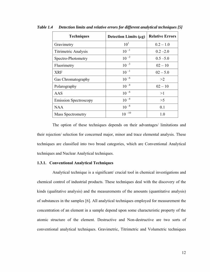
limits and relative errors for different analytical techniques are listed in Table 1.4.
12
Table 1.4 Detection limits and relative errors for different analytical techniques [5]
Techniques Detection Limits (g) Relative Errors
Gravimetry 101 0.2 – 1.0
Titrimetric Analysis 10 –1 0.2 –2.0
Spectro-Photometry 10 –2 0.5 –5.0
Fluorimetry 10 –3 02 – 10
XRF 10 –1 02 – 5.0
Gas Chromatography 10 –6 >2
Polarography 10 –4 02 – 10
AAS 10 –6 >1
Emission Spectroscopy 10 –4 >5
NAA 10 –8 0.1
Mass Spectrometry 10 –10 1.0
The option of these techniques depends on their advantages/ limitations and
their rejection/ selection for concerned major, minor and trace elemental analysis. These
techniques are classified into two broad categories, which are Conventional Analytical
techniques and Nuclear Analytical techniques.
1.3.1. Conventional Analytical Techniques
Analytical technique is a significant/ crucial tool in chemical investigations and
chemical control of industrial products. These techniques deal with the discovery of the
kinds (qualitative analysis) and the measurements of the amounts (quantitative analysis)
of substances in the samples [6]. All analytical techniques employed for measurement the
concentration of an element in a sample depend upon some characteristic property of the
atomic structure of the element. Destructive and Non-destructive are two sorts of
conventional analytical techniques. Gravimetric, Titrimetric and Volumetric techniques

13
fall in the group of the destructive technique. Some important non-destructive analytical
techniques, along with their principles, are mentioned below:
Polarography technique (measurement of voltage of electrolyte solution to obtain
current-voltage curve) [7]
Voltametry technique (measurement of current on a microelectrode at a specified
voltage)
Coulometry technique (measurement of current and time needed to complete an
electrochemical reaction or to generate sufficient material to react completely
with a specified reagent)
Potentiometry technique (measurement of the potential of an electrode in
equilibrium with an ion to be determined)
Conductimetry technique (measurement of the electrical conductivity of a
solution)
Visible Spectro-photometry (Colourimetry)
Ultraviolet Spectro-photometry technique (the absorption/ emission of radiant
energy and the measurement of the amount of energy of a particular wavelength
absorbed/ emitted by the sample)
Atomic Absorption Spectroscopy technique (vaporization of the specimen by
spraying a solution of the sample into a flame and then studying the absorption
of radiation from an electric lamp producing the spectrum of the element to be
determined) [8]
Atomic Emission Spectroscopy technique (submission of the sample to an
electric arc or spark so that atoms are raised to excited states causing them to
emit energy, which is measured)
Mass Spectrometry (on the basis of applied high voltage and mass to charge ratio
of ionized samples, obtained mass spectra)
X-ray Fluorescence Spectrometry (measurement of the wavelengths and their
characteristic intensities through x-ray spectra)
14
1.3.2. Nuclear Analytical Techniques
Nuclear analytical techniques are utilized for the analysis of the concentration of
elements in a wide diversity of materials and the composition of complex matrices. These
are extremely responsive methods for the trace elemental analysis and based on the
measurement of characteristic radiation emitted from radionuclides. By bombarding the
material with neutrons or charge particles (alpha particles, deuterons, protons etc.) or
gamma rays, the activation is provoked. They are applied for multi-elemental
determination in rocks, minerals, alloys, biological materials and environmental samples
such as water, air particulate matter, crops, vegetables, soil, sediments and diet. These are
also utilized to encompass a broader scope, which includes the production and
measurement of radio-isotopes in materials of known composition, for nuclear reaction
studies, for flux and beam intensities measurements of trace experiments and process
quality control. Some important nuclear techniques along with their principle are listed
below:
Activation Analysis (measurement of characteristic radiations emitted from radio-
nuclides which were formed directly or indirectly by activation)
Charge Particle Activation Analysis (sample is activated in accelerator with a
wide range of energies)
Photon Activation Analysis (-ray absorb to emit neutron with nuclear excitation
energy) [9]
Radio-chemical Neutron Activation Analysis (post irradiation chemical separation
occurs before Activation Analysis)
Neutron Activation Analysis (emission of characteristic -ray by the absorption of
thermal neutrons)
Instrumental Neutron Activation Analysis (involves irradiation and analysis of
samples in powder form without any chemical treatment)

15
Prompt -ray Neutron Activation Analysis (observe measurement readings during
irradiation of samples)
Delayed -ray Neutron Activation Analysis (measurements take place after
radioactive decay)
1.4. Neutron Activation Analysis (NAA)
With passage of time latest, sophisticated, sensitive, accurate and user-friendly
instruments are available in market for analyzing all feasible standard quality parameters.
Neutron Activation Analysis (NAA) is one of the most frequently utilized techniques for
elemental determination due to its high accuracy, specificity and multi-elemental analysis
capability. Due to its selectivity and sensitivity, NAA engage a significant place among
the various analytical methods performing both qualitative and quantitative multi-element
analysis of major, minor and trace elements in samples from almost every conceivable
field of scientific or technical interest [10-17]. It is an established powerful non-
destructive analytical technique for determination of concentrations at or below the ug/g
range, while up to 60 elements can be evaluated performing four irradiations processes
and several gamma-spectrum measurements after different decay periods. The major
fields of NAA application are analytical chemistry, geology, biology, life sciences and
industrial/ environmental pollution investigations. The utilization of purely instrumental
procedures for trace element analysis is commonly called instrumental neutron activation
Analysis (INAA) [18-22]. INAA is a method of analysis in which element specificity is
considered by employing appropriate irradiation conditions, radiation measurement
techniques and mathematical models for the interpretation of the results. With the use of
automated sample handling, gamma ray spectrum measurement with detectors and
computerized data processing, the sample may be recognized qualitatively and

16
quantitatively. Due to its superior sensitivities, NAA can determine many elements in the
order of parts per billion or better and in sample sizes from 10-5 to 10-1 gram. Moreover,
because of its accuracy and reliability, NAA is normally recognized, as the “referee
method” of choice when procedures are being developed or when other methods yield
results that do not agree. The physical phenomena upon which NAA is depending are the
properties of the nucleus, radioactivity and the interaction of radiation with matter. More
than about 70 elements can be investigated by this technique. At the 1ppm level, the
precision for many elements is about 3%. A majority of samples can be analyzed
without any preliminary preparation while aqueous samples are normally freeze-dried
before irradiation. NAA pursued by high-resolution gamma ray spectrometry has become
one of the promising and attractive analytical methods of simultaneous multi-element
analysis of biological and geological materials [23-27].
The series of events occurring during the nuclear reaction used for NAA,
namely the neutron capture or (n,) reaction is illustrated in fig. 1.1. A compound nucleus
is produced in an excited state due to unelastic collision of a neutron with the target
nucleus. Its excitation energy is due to the binding energy of the neutron with the nucleus.
The compound nucleus will almost immediately de-excite into a more stable form
through emission of one or more characteristic prompt gamma rays. In a majority of
cases, this new configuration yields a radio-active nucleus, which also de-excites (or
decays) by emission of one or more characteristic delayed gamma rays but at a much
slower rate according to the unique half-life of the radioactive nucleus. Due to the
particular radioactive species, half-lives can range from fractions of second to several
years.

17
Fig. 1.1 Neutron Activation Analysis Process
1.4.1. Sensitivity and Detection Limits of NAA
Neutron activation analysis is frequently applicable to the analysis of many
elements at pico-gram levels. The choice of chemical separation after irradiation is often
available for the blank-free removal of interfering materials. The technique is mainly
sensitive for the rare earth elements (e.g. Ce, La, Eu, Nd, Yb, Sm, Lu and Tb), Hf, Sc, Co,
Ta, Cr, Th, Cs, U and many others inorganic elements.
The sensitivities of NAA are based on following parameters:
The irradiation parameters (e.g. neutron flux, irradiation and decay times)
Measurement conditions (e.g. measurement time, detector efficiency)
Nuclear parameters (e.g. isotope abundance, neutron cross-section, half-life)

18
The calculated detection limits and sensitivity of NAA technique for different
metals are mentioned in Table 1.5 and 1.6 respectively.
Table 1.5 Calculated detection limits for neutron activation analysis [18]
Sr. No.
Elements Detection limit ( gm)
Sr. No.
Elements Detection limit ( gm)
1. Al 1 x 10⁻³ 21 Mg 1 x 10⁻¹
2. As 2 x 10⁻⁴ 22 Mn 6 x 10⁻⁵
3. Ba 6 x 10⁻² 23 Mo 2 x 10⁻²
4. Br 7 x 10⁻⁴ 24 Na 7 x 10⁻⁴
5. Ca 3 x 10⁻¹ 25 Nd 3 x 10⁻³
6. Cd 4 x 10⁻² 26 Ni 5 x 10⁻²
7. Ce 7 x 10⁻⁴ 27 Pb 2 x 100
8. Cl 3 x 10⁻⁴ 28 Rb 5 x 10⁻²
9. Co 5 x 10⁻⁵ 29 Sb 3 x 10⁻³
10. Cr 2 x 10⁻² 30 Sc 6 x 10⁻⁴
11. Cs 1 x 10⁻³ 31 Se 5 x 10⁻²
12. Cu 3 x 10⁻⁴ 32 Sm 3 x 10⁻⁴
13. Eu 2 x 10⁻⁶ 33 Sr 2 x 10⁻²
14. Fe 1 x 100 34 Ta 1 x 10⁻²
15. Hf 4 x 10⁻⁴ 35 Th 4 x 10⁻⁴
16. Hg 2 x 10⁻³ 36 Ti 1 x 10⁻²
17. I 4 x 10⁻⁴ 37 V 2 x 10⁻⁴
18. K 7 x 10⁻³ 38 Yb 7 x 10⁻⁴
19. La 2 x 10⁻⁴ 39 Zn 3 x 10⁻¹
20. Lu 4 x 10⁻⁵ 40 Zr 5 x 10⁻¹

19
Table 1.6 Sensitivity (g/g) of neutron activation analysis technique for metals [18]
Sr. No. Elements Sensitivity Sr. No. Elements Sensitivity
1. Aluminum (Al) 0.004 10. Magnesium (Mg) ND
2. Arsenic (As) 0.005 11. Manganese (Mn) 0.001
3. Calcium (Ca) ND 12. Sodium (Na) ND
4. Cadmium (Cd) 0.005 13. Nickel (Ni) 0.70
5. Cobalt (Co) 0.01 14. Lead (Pb) 0.5
6. Chromium (Cr) 0.3 15. Antimony (Sb) 0.007
7. Copper (Cu) 0.002 16. Selenium (Se) 0.01
8. Iron (Fe) 2.0 17. Tin (Sn) 0.03
9. Mercury (Hg) 0.003 18. Zinc (Zn) 0.1
1.4.2. Industrial Application of Neutron Activation Analysis (NAA)
In industrial application of Neutron Activation Analysis, the most significant
advantages involve the very low detection limits of elements, non-destructive and multi-
elemental analysis [28]. The matrices analyzed frequently comprise high purity and high-
tech materials, plastics, geological materials and such materials that are tricky to convert
quantitatively into a solution for subsequent analysis by other analytical techniques.
Various NAA methods have been developed for process research, testing, process control
and quality improvement.
The most common industrial applications or most regularly analyzed industrial
related matrices in which predominantly trace and ultra-trace concentrations of elements
were determined by various NAA procedures involve alloys, catalysts, ceramics and
refractory materials, coatings, electronic materials, detection of explosives, fossil and
other safeguard materials, fertilizers, graphite, integrated circuits, packing materials,
textile, dyes, semi-conductors, oil products and solvents, pharmaceutical products, silicon
processing. In the field of geology and geo-chemistry analyses of a variety of substances

20
have been frequently performed such as asbestos, borehole samples, bulk coal and coal
products, crude oils, kerosene, petroleum, cosmos-chemical samples, cosmic dust, coral,
diamonds, meteorites, ocean nodule, rocks, sediments, soil, glacial till, ores and minerals.
1.4.3. Advantages of NAA
NAA has become a base for geo-chemical and bio-chemical trace elemental
analysis because the technique owns several important advantages. Some salient ones are
listed below:
1. It is appreciably sensitive technique among multi-element analysis methods
2. More than 35 elements can be determined simultaneously, from parts per billion to percentage concentration
3. Little or no sample preparation is required and hence no blank reagent values are involved
4. High specificity is achieved via sophisticated computer program
5. Matrix interference effects are rare and good precision level (below 1%) is achieved
6. Owing to the low detection limits, small size samples are sufficient for analysis
7. Intermediate steps such as dissolution and separation are not necessary because chemical treatment is not required
8. There is substantial freedom from systematic errors
1.4.4. Limitations of NAA
There are a few limitations of NAA such as
1. Nuclear reactor is its basic requirement
2. The elapsed time for an analysis of long lived radionuclides can be 4-6 weeks
3. The radiation hazards involved also make it a less attractive technique
4. The highly active matrix nuclides (e.g. 24Na, 42K, 82Br, 32P etc) interfere with long- lived radionuclides (e.g. Cu, As, Mo, Cd, Zn, Sb, Co, Fe, Cr, Hg, Se etc.)

21
1.5. Atomic Absorption Spectroscopy (AAS)
The principle of atomic absorption spectroscopy (AAS) depends on the
absorption of light energy by atoms and follows Beer’s Law. A distinct amount of energy
is absorbed and re-emitted by an atom and after absorbing a quantum of energy, the atom
is transformed into a particular energy excited state. The atom generally releases the
absorbed energy in the form of radiations after de-exitation. The technique recommends
low detection limits for most of the elements [29-31]. Due to detection limits, flame
Atomic Absorption Spectroscopy has been substitute by Non- flame Atomic Absorption
Spectroscopy, which has graphite furnace instead of flame. The quantitative evaluation
can be carried out by comparison with reference substances. The physical interferences
are produced by differing physical properties of the sample and the reference substance,
such as different viscosities, surface tensions or specific gravities of the solutions or
solvents. Sample dissolution procedures may face some contamination problems. Hence,
this technique is not appropriate for high purity materials and for those samples with low
elemental concentration. In addition, direct introduction of solid samples into the flame
brings diversity of problems.
1.5.1. Theoretical Aspects of AAS
Atomic absorption spectroscopic method is depending on the relationship
between the concentration of an element and the intensity of absorbed light. Two
fundamental laws i.e. Lambert and Beer’s laws rule the absorption of monochromatic
radiations by homogenous clear solution. In AAS, the absorption of light “A” is
associated to the path length and number of ground state atoms as shown by following
equation [5]:

22
A = log (I0/ It) = K N0 L
Where
I0 = Intensity of the incident light It = Intensity of the transmitted light K = Absorption coefficient N0 = Number of ground state atoms per cm3 L = Path length through the flame (cm)
For a fix path length, the absorption will be a linear function with the number of
atoms (concentration) at ground state of up to a certain level. At higher absorption
values, deviations from the law will observe.
1.5.2. Advantages of AAS
Some salient advantages of AAS are losted below:
1. AAS is famous for its simplicity, ease of use, capable of analyzing for a wide range of elements in a variety of matrices and high sensitivity
2. The technique offers low detection limits for majority of the elements
3. For hydride forming elements such as arsenic and selenium, great sensitivity is obtained by generating the volatile hydrides
4. Reducing of Hg (II) compounds to produce elemental mercury vapours also give an extremely sensitive method for quantitative determination of mercury
1.5.3. Limitations of AAS
Some major limitations are listed below
1. Due to chemical interference, 30 elements (e.g. lanthanides, aluminum, silicon, boron, uranium etc.) cannot be determined in air/ acetylene flame due to formation of stable metal oxides. Similarly, the elements in sub group IV, V, tungsten and several other elements can be determined with relatively low sensitivities.
2. Some physical and organic interference also control the use of AAS for trace element analysis of many matrices and solutions.

23
3. Various elements are more or less strongly ionized, especially in hot flames producing ionization interferences, which bring reduction in the sensitivity.
4. A separate hollow cathode lamp is desired for each element. Some of them are very costly and have short lifetime of 100 operation hours only.
5. Two major limitations apply to all the atomic spectroscopic methods. First, they have restriction to distinguish among oxidation states and the chemical setting of the analyte elements. Second, they are insensitive to non-metallic elements.
1.5.4. Sensitivity and Detection Limits of Atomic Absorption Spectrometric technique
AAS technique has reasonable sensitivity and detection limits for the analysis of
elements, which are generally present in pollution environment. The sensitivity and
detection limits for such elements are listed in following Table. 1.7.
Table 1.7 Sensitivity (g/g) and Detection Limits (g/g) of AAS techniques [5]
Elements Sensitivity Detection Limits
Elements Sensitivity Detection Limits
Al 0.8 3 x 10⁻² Mn 0.02 2 x 10⁻³
As 0.8 1 x 10⁻¹ Mo ND 3 x 10⁻²
Ca 1.0 1 x 10⁻³ Na ND 2 x 10⁻³
Cd 0.01 1 x 10⁻³ Ni 0.07 5 x 10⁻³
Co 0.07 2 x 10⁻¹ Pb 0.1 1 x 10⁻²
Cr 0.06 3 x 10⁻³ Sb 0.3 ND
Cu 0.04 2 x 10⁻³ Se 0.5 ND
Fe 0.06 5 x 10⁻³ Sn 1.0 2 x 10⁻²
Hg 2.2 5 x 10⁻¹ Zn 0.009 2 x 10⁻³
Mg ND 1 x 10⁻⁴

24
CHAPTER – 2
2. Literature review
In various under-developed countries, untreated sewage and industrial effluents
are utilized for the cultivation of crops and vegetables [32]. It is a frequent practice in the
industrial cities of Pakistan also [33] because farmers suppose it a source of irrigation and
nutrients for cultivation [34] while administrators assume it a low cost method of
disposal. Unprocessed effluents contain heavy metals, microorganisms and organic
pollutants [35]. Problems arise due to the increase of metal ions in biosphere with
continuous application onto soils. These metals have toxic impact on metabolism of
living organisms when they exist beyond their respective safe limits in soils, vegetables
and crops. These metals get their way, through food chain, in the bodies and produce
health hazard effects on animals and human beings. According to the surveys, from
public health services of under developed countries, large number of people has been
exposed to health hazards of excess metals through municipal water supplies [36-38]. The
increasing amounts of toxic metals emitted into the biosphere, as a result of fast
industrialization and urbanization, cause permanent threatening to the ecosystem also.
Thus the main objective of the proposed project was to identify the pollutants in the
industrial effluents and their treatment through reliable and economical technique to
minimize the industrial pollution.
2.1. Industrial effluents
Numerous studies [39-41] have been conducted to characterize the city and
industrial effluents for cultivation with respect to Electrical Conductivity (EC), Sodium
Adsorption Ratio (SAR), Residual Sodium Carbonate (RSC) and metal ion concentration.

25
Ghafoor et al [34] concluded that the effluents of Faisalabad city were unfit for irrigation
purposes due to high EC and RSC. However, the concentrations of metals (Fe, Mn, Cu,
Zn, Pb and Ni) were within the safe limits. Ibrahim et al [32] also decided that the
effluents of Faisalabad were unfit for cultivation regarding EC, SAR and RSC.
Concentration of Cd, Fe, Cu, Pb and Mn ranged between 0.051-0.054, 1.78-1.85, 0.34-
0.58, 0.39-0.63 and 0.18-3.07 mg/l respectively in the city effluents, according to the
results of Khan et al [35]. Ali [42] reported pollution of River Ravi from Lahore city
where the concentration of Cr, Cu, Pb, Mn, Hg, Ni and Cd at the main out fall was 1.29,
1.20, 1.10, 2.00, 0.003, 0.006 and 0.007 mg/l respectively. It was concluded by many
researchers [32-34] that the concentrations of Cd, Cr, Cu and Mn in the effluents of
Faisalabad’s industries were higher than the recommended values. Sewage being used to
grow vegetables and crops in India was also assessed [43]. Manzoor et al [44] estimated
heavy metals by AAS in textile effluents. They concluded that the concentrations of Cr
(5.96 mg/Kg) and Pb (4.46 mg/Kg) were dominant in the effluents. Various scientists [45-
54] had performed treatment of industrial effluents through different methods. Babursah
et al [55] and Gyliene et al [56] had removed certain metals using filters. Similarly many
researchers [57-60] had removed heavy metals by the use of husks.
2.2. Agricultural soils
According to various researchers [61-65], industrial effluents have been applied
onto agricultural soils as a suitable mean of disposal but it resulted in the contamination
of soils with a wide range of metals. Ghafoor et al [66] reported higher accumulation of
metals (Fe, Mn and Zn) in sewage receiving soils than those irrigated with canal water.
Singh et al [67] concluded that extractable metals (Fe, Cu, Zn, Mn, Pb, Cd and Cr) were

26
comparatively higher in soils being continuously irrigated with city sewage in India. The
behavior of trace metals in soils depends on the level of contamination and properties of
soils like pH, texture, type of clay, lime contents and organic matter [68-73]. Solubility of
heavy metals in soils as a function of pH is often guided by the presence of organic and
inorganic ligands [74-77]. Generally, addition and availability of metals from
anthropogenic sources are more than those from soil parent material, particularly in the
third world countries [78-82]. Soils enrich in clay-sized minerals tend to retain a higher
concentration of trace elements. Most of the trace metals have a low mobility in soils
because they get adsorbed strongly on soil minerals and organic matter or from insoluble
precipitates as oxides, carbonates and sulphides [83-85]. Even in well-drained sandy loam
soils, maximum concentration of metals (Fe, Mn and Zn) was observed in upper (30 cm)
soil layer near Faisalabad receiving sewage irrigation for the last 2-3 decades [66].
Ghafoor et.al [86] concluded that almost all the surface layers of several sewage-irrigated
soils contained higher concentration of metals (Cd, Pb, Cr, Cu, Zn, Mn and Fe).
Comparatively less concentration of these metals in lower soil horizons was attributed to
their lower mobility. The concentration of Mn, Cd and Co tended to decrease with an
increase in the soil depth [87-90]. A comprehensive review data for last 30 years [91]
indicated that the soil irrigated with Faisalabad city effluents had attained concentration
of Cu, Fe, Mn and Zn beyond their respective permissible limits.
2.3. Vegetables
Growing vegetables and crops with industrial effluents for longer periods may
guide to accumulate the trace metals in soils up to toxic levels. This could be of particular
importance where vegetables are grown [66]. Vegetables sampled from pollutant free

27
areas contained concentrations of metals at permissible levels [91]. Spinach and
cauliflower grown with canal water had better-looking quality and taste than irrigated
with effluent [92]. Normally, vegetables grown on sewage/ effluents applied soils
accumulated high concentration of metal ions like Cd, Cu, Ni, Pb and Zn [43]. Qadir et al.
[93] presented a comprehensive review about the metal poisoning in more than 12
vegetables, irrigated with city effluent. Ado-Ekiti [94] observed that concentration of Cu,
Pb and Zn in lettuce, tomato stalk, leaves and fruit tissues generally increased in the
Granby and fox soils. In general, correlation between concentration of metals in soils and
vegetables is said to be unpredictable [89]. They reported that not only species differed
significantly but also different anatomical parts of the same species changed in level of
contamination with Pb and Cd. Concentration of Pb and Cd was maximum in leaves
(Spinach lettuce) followed by root and tuber (radish & carrot), cabbage (various types of
cabbages & cauliflower), bulb (onion & garlic) and fruits (tomato & nipper green bean).
Boom et al [95] found the same patern for lettuce, potato, radish and carrot along with
eighty vegetable samples. Heavy metals (Mn, Cd and Co) tended to accumulate more in
leaves than their respective fruits of okra, bitter guard, mint and spinach [87]. The
vegetables cultivated with fresh water in different countries of the world such as Pakistan
[96-97], Iraq [98], Italy [99], Poland [100], China [101] and India [28, 102] were
analyzed for major, minor and trace elements and were found contamination free, with a
couple of exceptions. Fardy et al [103] determined the concentration of Manganese in
Australian vegetables such as pumpkin, potato, carrot etc. The city effluent is a big source
of heavy metals [65, 104].like Cd, Cr, Ni and Zn, which may accumulate in the edible
portion of the vegetables and cause different diseases through human food chain.

28
2.4. Crops
Various workers have reported the elemental concentrations for the crops such
as Wheat [41, 98, 105], Maize [106-107] and Rice [28, 105, 108]. Field data from
Chicago district [109] indicated that crop tissue metal (Cd, Cu & Zn) concentration was
dependent on soil pH and increased at a low metal loading (50, 200, 750 g/gm
respectively). Four categories of metals have been observed for partitioning the plant
parts i.e. (a) Pb, Sn, Ti, Ag, Cr, Zn, Ca, As and Be mostly accumulated in roots with a
little quantity in shoot, (b) Fe, Cu, Al, Cd, Co, Mo and Si mostly accumulated in roots
with a substantial quantities in shoot, (c) Zn, Mn, Ni and Se were almost uniformly
distributed in root and shoot and (d) B, Li and some times Mn mostly accumulated in
shoot. However, these effects differed somewhat with plant species. This has the
implication that plants, grown on soils where effluent has been applied in the past, are
likely to accumulate even greater metal contents in the event of a rise in atmospheric
temperature Hooda et al [110]. The requirement of essential elements is necessary to
maintain the human health. The bioavailability of Zinc element from Pakistani cereals
(wheat and rice) grains is more than sufficient for human consumption [105]. The
concentration of Manganese was determined in Australian diet (wheat, rice and maize) by
Fardy et al [103] to evaluate its dietary intake values. Selenium concentration was high in
corn samples collected from China [107]. Similar results were obtained [111] for the
analysis of toxic/ trace elements in wheat, rice and maize samples. Various researchers
[41, 67, 106, 112-118] had determined major and minor elements in crops (wheat, rice
and maize) to evaluate their toxic level and nutrition values in them.

29
CHAPTER-3
3. Aims and Scope
The present research work is in the field of industrial pollution, which is a
current burning topic. The control of the pollution is imperative to improve the human
health and to clean the environment. The prime aims of this research are to investigate the
harmful pollutants in effluents, agricultural soil, crops, vegetables and their treatment to
reduce the pollution. This study gives detailed information about the pollution sources
and their hazardous impacts on the aquatic life/ animals/ human beings. In this regard, a
variety of polluted crops and vegetables have been analyzed which indicated the presence
of metal poisoning, above the recommended permissible level by WHO. Suitable,
economical and reliable treatment techniques have been used to check the pollution
parameters. This research will be beneficial to minimize the industrial pollution by the
immobilization of the toxic constituents in the effluents.
3.1. Motivation
Industrial pollution in Pakistan is growing at a faster rate and is a serious threat
to its economy as well as human health. Pollutants that degrade air, water and soil make it
difficult for environment to sustain long-term developments. The problems related to
industrial pollution and the need to protect/ preserve the environment from further
deterioration have largely drawn attention of scientists and environmentalists of the
country. Effective measures, which can eliminate or considerably reduce hazardous
factors from the human environment to minimize the associated health risks, must be
identified and eradicated collectively. Moreover, sufficient database is not available,
presently in Pakistan, pertaining to the concentration of metals in the industrial effluents

30
and their accumulation in soil, crops and vegetables. In order to achieve these objectives,
suitable experimental modeling and analysis techniques need to be applied to reach a
balanced assessment of the risks and benefits involved. Enforcing the environmental
protection laws and public awareness can control the situation. It will not only lead to a
clean Pakistan but also make it a healthy place to live.
3.2. Research Objectives
Following are the three main objectives for the study of industrial effluents,
agricultural soils, crops and vegetables with reference to the pollution:
Identification of the pollution sources
Estimation of the industrial toxic levels
Treatment of the industrial effluents
3.3. Work Plan
To study pollution, induced in the ecosystem of the industrial cities by the
effluents, the salient points were as follows:
Extensive literature survey was carried out in order to update the current status
of the problem in Pakistan
Survey of the selected industrial cities i.e. Faisalabad and Gujranwala was done
to build a database regarding the relevant particulars of industries under
investigation and the ecology of the vicinity of the industrial areas. Faisalabad
and Gujranwala from Punjab Province were chosen as industrial cities because
there were 288 ceramics, 51 Pulp/ paper and 5786 textile industries in
Gujranwala division while 72 Pulp/ paper and 11348 textile industries were
present in Faisalabad division. There was no Ceramics industry in Faisalabad.
Industrial effluents from Textile/ Yarn, Pulp/ Paper and Ceramics industries
were collected for the determination of toxic inorganic elements contaminating
the ecosystem of the industrial cities

31
The specimens of the irrigated soil exposed to the industrial effluent, used for
cultivation, were collected to study the contamination levels
The crops and vegetables, grown on the effected soils, were collected to
determine the degree of trace metal contents in them
The procedures were optimized for the application of Neutron Activation
Analysis (NAA) and Atomic Absorption Spectrometric (AAS) techniques to
carry out these studies
On the basis of the data obtained and its interpretation, procedures were
developed to decontaminate the effluents from the toxic inorganic elements and
to make them immobilize
3.4. Working Strategy
The proposed work has been performed with the help of available/ existing facilities
such as 10 MW Research Reactor (PARR-I), Zero Power Research Reactor (PARR-II),
High Resolution γ-ray Spectrometric System, Atomic Absorption Spectrometer, Pentium-
IV PC for data processing utilizing different software packages, Freeze dryer, Incubator,
Laminar flow, Hot cell and Analytical facilities i.e. pH meter, Conductivity meter, Titrino
Unit, TDS meter, Turbidity meter etc
3.4.1. Sampling and Sample Preparation
Samples from the effluents of the four industries selected for this study were
collected along with the samples of soil, crops and vegetables from the vicinity of
the industrial areas
All samples were prepared according to the requirements of the techniques used,
i.e. NAA or AAS, for the analysis
Each species of vegetable and crop sample was separated into its fruits, flowers,
leaves, stems and roots to evaluate the bio-distribution of trace elements, in each
portion

32
The samples of crops and vegetables were washed, freeze-dried, crushed, sieved
and homogenized
All the samples so prepared, along with the synthetic/ secondary reference
materials, were encapsulated in polyethylene or aluminum capsules according to
the recommended time of irradiation
For NAA, the samples of the effluent were dried to form a homogeneous
powder
For AAS, the samples of soil, vegetables and crops were digested, along with
the synthetic/ secondary reference materials to form clear solutions
3.4.2. Analysis
i) For NAA, following parameters were optimized in order to get best results:
Time of irradiation
Cooling time
Counting time
Determination of variations in neutron flux gradient
ii) For AAS different experimental parameters were optimized, according to
the requirements of an element under investigation
3.4.3. Data Processing
The experimental readings obtained were processed for the
determination of concentrations of different inorganic elements in the
samples of different matrices
The data were interpreted to draw conclusion with reference to the
hazardous effects of these anthropological activities on human life
3.4.4. Decontamination Procedures
The decontamination methodologies of the industrial effluents from
the toxic inorganic elements were investigated
The optimized method was developed to immobilize the toxic elements

33
CHAPTER-4
4. Experimental Work
Experimental work is planned with different steps in a systematic sequence for
the qualitative and quantitative determination of major, minor and trace elements present
in the samples of crops, vegetables, soils and industrial effluents. The important steps like
sample collection, preparation, irradiation and analysis are described here in detail.
4.1. Sampling
Soil sampling was completed according to prescribed standard procedures [81].
The weather conditions e.g. rain, sun shining, cloudy day, wind blowing and other
important features at the time of sampling were also indicated. The frequency and type of
samples from suitable sampling locations were mentioned. Sampling equipments and
current methods of sample preservation were also revealed. Sampling was performed, in
different seasons, for the collection of crops, vegetables and soil samples. All possible
parameters were considered during work to minimize the errors. All collected samples
were about 01-03 km away from the selected industries. All samples were transported
carefully to the laboratory site for their preparation and analysis.
4.1.1. Sample Collection
The Grab sampling technique was utilized for the collection of samples of soil,
crops and vegetables. 406 soil samples were collected with the aid of a Shovel. from
those areas in Faisalabad and Gujranwala which were irrigated with effluents. Before
collection of soil samples, superficial layer from topsoil was removed to avoid
unnecessary contaminations, which was fallout from the atmosphere. The sample

34
collection sites of Faisalabad [119] and Gujranwala [120] areas are mentioned in Fig. 4.1
and 4.2 respectively.
Fig. 4.1 Samples collection sites plan of Faisalabad areas

35
Fig. 4.2 Samples collection sites plan of Gujranwala areas
The Composite sampling technique was adapted for the collection of industrial
effluents from a specific location at different times. In this regard, 325 effluents samples
of textile, 118 effluents samples of ceramics and 139 effluents samples of pulp/ paper
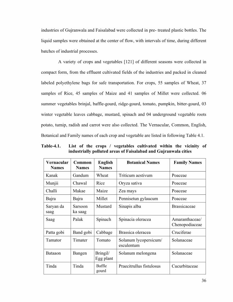
36
industries of Gujranwala and Faisalabad were collected in pre- treated plastic bottles. The
liquid samples were obtained at the center of flow, with intervals of time, during different
batches of industrial processes.
A variety of crops and vegetables [121] of different seasons were collected in
compact form, from the effluent cultivated fields of the industries and packed in cleaned
labeled polyethylene bags for safe transportation. For crops, 55 samples of Wheat, 37
samples of Rice, 45 samples of Maize and 41 samples of Millet were collected. 06
summer vegetables brinjal, baffle-gourd, ridge-gourd, tomato, pumpkin, bitter-gourd, 03
winter vegetable leaves cabbage, mustard, spinach and 04 underground vegetable roots
potato, turnip, radish and carrot were also collected. The Vernacular, Common, English,
Botanical and Family names of each crop and vegetable are listed in following Table 4.1.
Table-4.1. List of the crops / vegetables cultivated within the vicinity of industrially polluted areas of Faisalabad and Gujranwala cities
Vernacular Names
Common Names
English Names
Botanical Names Family Names
Kanak Gandum Wheat Triticum aestivum Poaceae
Munjii Chawal Rice Oryza sativa Poaceae
Challi Makae Maize Zea mays Poaceae
Bajra Bajra Millet Pennisetun gylaucum Poaceae
Saryan da saag
Sarsoon ka saag
Mustard Sinapis alba Brassicaceae
Saag Palak Spinach Spinacia oleracea Amaranthaceae/ Chenopodiaceae
Patta gobi Band gobi Cabbage Brassica oleracea Cruciferae
Tamator Timater Tomato Solanum lycopersicum/ esculentum
Solanaceae
Bataaon Bangen Bringil/ Egg plant
Solanum melongena Solanaceae
Tinda Tinda Baffle gourd
Praecitrullus fistulosus Cucurbitaceae

37
Kali Tori Tori Ridged gourd
Luffa acutangula Cucurbitaceae
Karayla Karayla Bitter gourd
Momordica charantia Cucurbitaceae
Ghiya Kaddu Pumpkin Cucuabita maxima/ pepo Cucurbitaceae
Aalo Aalo Potato Solanum tuberosum Solanaceae
Thipper Shalgum Turnip Brassica rapa rapa Brassicaceae
Molian Moli Radish Raphanus sativus Brassicaceae
Gajaran Gajer Carrot Daucus carota Apiaceae
The large size/ volume samples [27] of soil, crops, vegetables and effluents
were obtained through grab and composite sampling techniques. One-kilogram sample
[23] was collected, beneath the super-facial layer of the soil. Another one-kilogram
sample was collected from one foot deep, on the same site and both were packed
separately, in proper sized-labeled Polythene bags. Crop and vegetable samples of one-
kilogram each were collected in different seasons. Each effluent sample with a volume of
500-600 milli-liters was collected to perform all the required analysis plus any quality
control need, split samples or repeat examinations.
4.1.2. Samples Preservation
Sample preservation techniques such as addition of chemicals, pH control (e.g.,
for metal analysis the pH of the samples should be less than 2), refrigeration (temperature
up to 4 C) etc., were utilized. These steps were significant to attain the following targets:
i. To minimize the biological activities
ii. To retard hydrolysis of chemical compounds and complexes
iii. To reduce the volatility of the constituents
iv. To stabilize the desired parameters for long period before analysis

38
4.1.3. Sample Preparation
Sample preparation procedures and equipments [26] were quite different
depending upon the type of the sample under investigation. The purpose of sample
preparation was to trim down the size of a representative sample of required material to
be chosen for analysis. During sample preparation, plastic disposable gloves were worn to
protect further contamination in all the samples. Each soil sample was dried separately, in
an oven, for about 24 hours at 50 –60 ºC to defend the losses of more volatile elements
such as Mercury. After complete dryness, possible contaminated materials such as root,
stones, bricks, cotton, pieces of paper etc. were physically removed to decontaminate the
soil sample. In order to obtain same size of the grains, the clay/ silt/ sand samples were
crushed, in mortar, into fine powder. In sieve shaker, fine powder was scanned
thoroughly, for uniform particle (260-micron meter) size grading. Polythene or Nylon
sieves and Teflon mortar were utilized to avoid iron contamination in the samples. The
homogeneous, mono-grade powder was assembled in proper sized plastic containers with
screw caps.
For the collection and storage of effluent samples [122-123], pre-treated acid
cleaned high-density polyethylene bottles were engaged. Plastic containers were
permeable to Oxygen, Carbon dioxide and Mercury vapours. Therefore, physical
parameters (such as pH, temperature, density, electrical conductivity, specific gravity,
TDS and turbidity) of the effluent were determined within a possible short time and then
it was dried to protect from further contamination before chemical analysis. Slow heating
was performed to avoid evaporation of volatile compounds from the samples.

39
One selected most important species of crop/ vegetable was separated from all
other minor species. Fruits, flowers, leaves, stems and roots were separated from one
another. All parts were washed thoroughly with tap water for about 8–10 times. These
parts were again washed thoroughly with distilled water for about 2 times to remove all
minor traces of clay, silt, sand or any other contamination. Each part was dried separately,
in an incubator (BE-200, Memmert, Germany), at 50 –59 ºC for about 24 hours. After
complete dryness, the sample was crushed in grinder (Moulinex)), into fine powder.
Homogenization of each sample was done to get uniform results. The powder was then
collected in proper sized plastic containers with screw caps.
4.1.4. Sample Identification
A large number of samples were collected from same location and occasion. So a
specific code number identified each sample. Sample classification information such as
origin of sample, sampling station, location, date, weather, sampling techniques, sampling
procedures, field observations and remarks were also recorded to make clear the protocols
of the sampling. Each prepared container of sample was labeled with a specific number.
After affixing appropriate codes and notations on them, all samples were stored in a dark,
cool and clean (with out any chemicals) storeroom to protect them from further
contaminations.
Crops (178), vegetables (102) and soil (406) samples were collected from
twenty-four different industrial areas of Faisalabad/ Gujranwala. Ceramics (118), Textile/
yarn (325) and Pulp/paper (111) industrial effluents from different locations were also
collected. Proper codes and notations were allotted for their identification as shown in
Tables 4.2, 4.3 and 4.4 for all crops/ vegetables, soil and industrial effluents respectively.

40
Table 4.2 Codes for samples of the crops and vegetables For city code
Sr. No. CITIES CODE 01. 02.
FAISALABAD GUJRANWALA
F G
For places/ locations
Sr. No.
PLACES (Faisalabad))
Zones Sr. No.
PLACES (Gujranwala)
Zones
01. 02. 03. 04. 05 06
Industrial Estate Ghulam Muhammad-abad Peoples Colony Sitara Colony Nishatabad Gulistan Colony
F – 1 F – 2 F – 3 F – 4 F – 5 F – 6
07. 08. 09. 10. 11. 12.
Dhule Garjakh Small Industrial Estate Muhammad – Nagar Fatomand Satellite Town
G – 1 G – 2 G – 3 G – 4 G – 5 G – 6
Note: When more than one sample was collected from different locations of the same
place then a star “ * ” was added with it.
For crops/ vegetables
Sr. No. SPECIES CODES Sr. No. SPECIES CODES
01. WHEAT i 10. TURNIP x 02. RICE ii 11. BRINJAL xi 03. MAIZE iii 12. Baffle Gourd xii 04. MILLET iv 13. Ridged Gourd xiii 05. MUSTARD v 14 RADISH xiv 06. POTATO vi 15 Bitter Gourd xv 07. SPINACH vii 16 CARROT xvi 08. CABBAGE viii 17 PUMPKIN xvii 09. TOMATO ix
For parts of the crops/ vegetables
Sr. No. PARTS CODES
01. 02. 03. 04. 05.
FRUITS/ LEGUMES FLOWERS LEAVES STEMS ROOTS
F FL L S R
FORMULA: City + Place + Star + Species + Part
G3vL Along with sampling Date

41
Table 4.3 Codes for samples of the soil
For Cities
FOR CITY CODE: FOR DEPTH OF SOIL:
Sr. No.
CITIES CODE Sr. No.
DEPTH CODE
01. FAISALABAD F 01. Sample of topsoil St 02. GUJRANWALA G 02. Sample of subsoil Ss
For places/ locations
Sr. No.
PLACES (Faisalabad))
Zones Sr. No.
PLACES (Gujranwala)
Zones
01. 02. 03. 04. 05 06
Industrial Estate Ghulam Muhammad-abad Peoples Colony Sitara Colony Nishatabad Gulistan Colony
F – 1 F – 2 F – 3 F – 4 F – 5 F – 6
07. 08. 09. 10. 11. 12.
Dhule Garjakh Small Industrial Estate Muhammad – Nagar Fatomand Satellite Town
G – 1 G – 2 G – 3 G – 4 G – 5 G – 6
Note: When more than one soil sample was collected from different locations of the same
place then a star “ * ” was added with it. For crops/ vegetables
Sr. No. SPECIES CODES Sr. No. SPECIES CODES
01. WHEAT i 10. TURNIP x 02. RICE ii 11. BRINJAL xi 03. MAIZE iii 12. Baffle Gourd xii 04. MILLET iv 13. Ridged Gourd xiii 05. MUSTARD v 14 RADISH xiv 06. POTATO vi 15 Bitter Gourd xv 07. SPINACH vii 16 CARROT xvi 08. CABBAGE viii 17 PUMPKIN xvii 09. TOMATO ix
FORMULA: City + Place + Star + Depth + Crop Species
G 1 A iii Along with sampling Date

42
Table 4.4 Codes for samples of the industrial effluents
For city code
Sr. No. CITIES CODE
01. 02.
FAISALABAD GUJRANWALA
F G
For places/ locations
Sr. No.
PLACES (Faisalabad))
Zones Sr. No.
PLACES (Gujranwala)
Zones
01. 02. 03. 04. 05 06
Industrial Estate Ghulam Muhammad-abad Peoples Colony Sitara Colony Nishatabad Gulistan Colony
F – 1 F – 2 F – 3 F – 4 F – 5 F – 6
07. 08. 09. 10. 11. 12.
Dhule Garjakh Small Industrial Estate Muhammad – Nagar Fatomand Satellite Town
G – 1 G – 2 G – 3 G – 4 G – 5 G – 6
Note: When more than one effluent sample was collected from different locations of the same place then a star “ * ” was added with it.
For industries:
Sr. No. INDUSTRIES CODE
01. 02. 03. 04.
CERAMICS PAPER TEXTILE YARN
C P T Y
FORMULA: City + Place + Star + Industry G 1 C Along with sampling Date
4.2. Reference Materials for NAA
Any homogeneous material with recognized concentrations of appropriate
elements is classified as multi-element reference/ standard material. All Standard
Reference Materials (SRM) are purposely-prepared materials, which are composed of
definite concentrations of the elements. The technique of Instrumental Neutron Activation
Analysis (INAA) was utilized by adopting comparator/ relative method for the

43
determination of concentration of elements without any pretreatment of the samples.
Excellent standardization is the basic requirement for the accuracy of any analytical
facility so SRMs are regularly used in most laboratories for calibration of the
measurement processes. Such standards were obtained from different certifying
authorities like National Bureau of Standards (NBS), International Atomic Energy
Agency (IAEA) and various other commercial sources. Descriptions of geological and
biological reference materials (Standards) along with their elements, which were used for
this work, are given in Table 4.5.
Table 4.5 Description of geological & biological reference materials/ Standards
Supplier Code Material Unit Wt.
Elements of cited/ informative values
IAEA IAEA/ SL-1
Lake Sediment
25 gm Ag, Al, As, Au, Ba, Br, Ca, Cd, Ce, Cl, Co, Cr, Cs, Cu, Dy, Eu, Fe, Ga, Ge, Hf, Ho, Hg, I, In, K, La, Lu, Mg, Mn, Mo, Na, Nb, Nd, Ni, Pt, Rb, Ru, Sb, Sc, Se, Sm, Sn, Sr, Ta, Tb, Te, Th, Ti, U, V, W, Y, Yb, Zn, Zr
IAEA IAEA/ S-7
Soil 25 gm Al, As, Ba, Br, Ca, Cd, Ce, Co, Cr, Cs, Cu, Dy, Eu, F, Fe, Ga, Hf, Ho, Hg, K, La, Lu, Mg, Mn, Mo, Na, Nb, Nd, Ni, Rb, Ru, Sb, Sc, Se, Si, Sm, Sr, Ta, Tb, Th, Ti, U, V, Y, Yb, Zn, Zr
NBS NBS/ SRM-1572
Citrus Leaves (CL)
70 gm Al, As, Ba, Br, Ca, Cd, Ce, Cl, Co, Cr, Cs, Cu, Eu, Fe, Hg, I, K, Lu, Mg, Mn, Mo, Na, Ni, Rb, Sb, Sc, Se, Si, Sm, Sn, Sr, Te, Ti, U, Zn
IAEA IAEA-336
Lichen 20 gm Al, As, Ba, Br, Cd, Ce, Cl, Co, Cr, Cs, Cu, Eu, Fe, Hg, K, La, Lu, Mn, Na, Nd, P, Pb, Rb, Sb, Sc, Se, Sm, Sr, Tb, Th, V, Yb, Zn
IAEA IAEA-155
Whey Powder (WP)
50 gm Al, As, B, Br, Ca, Cd, Cl, Co, Cr, Cs, Cu, Fe, Hg, K, Mg, Mn, Na, Ni, P, Pb; Rb, S; Sc, Se, Sr, Zn

44
For trace elemental analysis, the certified reference materials utilized, for the
study of geological samples, were Soil (IAEA-S 7) and Lake Sediment (IAEA-SL 1),
both supplied by IAEA. SL-1 was collected from the Sardis Reservoir, Mississippi, USA.
For the analysis of biological samples (crops and vegetables), three other types of
standards were consumed for trace elemental analysis. The one certified reference
material engaged was Lichen (IAEA-336) {Date/ Batch No. 1994/ 56} and was supplied
by IAEA. The other selected certified reference material was Citrus Leaves (NBS/ SRM-
1572) and was supplied by National Institute of Science and Technology (NIST), USA.
The third certified reference material was Whey Powder (IAEA-155) {Date/ Batch No.
1990/ 100} and was supplied by IAEA. Whey Powder (WP) is the dried material of water
extracted from the split milk. The cited/ informative values of elements for all five
standard materials (SRM/CRM), used for the work, are listed in Table 4.6.
Table 4.6 IAEA Reference sheets (1999 & 2000) for cited values of Biological (Lichen, CL & WP) and Geological (SL-1 & S-7) standards
Sr. No.
Elements Lichen (ppm)
CL (ppm)
Whey Powder WP
(ppm)
SL-1 (ppm)
S-7 (ppm)
1. Al 0680.0000 00092.0000 00052.900 89000.00 047000.00
2. As 0000.6300 00003.1000 00000.049 00027.50 000013.40
3. Ba 0006.4000 00021.0000 00639.00 000159.00
4. Br 0012.9000 00008.2000 00039.100 00006.82 000007.00
5. Ca 31500.0000 42100.000 02500.00 163000.00
6. Ce 0001.2800 00000.2800 00117.00 000061.00
7. Cl 1900.0000 00414.0000 69200.000 00010.00
8. Co 0000.2900 00000.0200 00000.043 00019.80 000008.90
9. Cr 0001.0600 00000.8000 00000.590 00104.00 000060.00
10. Cs 0000.1100 00000.0980 00000.086 00007.01 000005.40
11. Cu 0003.6000 00016.5000 00000.570 00030.00 000011.00
12. Eu 0000.0230 00000.0100 00001.60 000001.00

45
13. Fe 0430.0000 00090.0000 00062.000 67400.00 025700.00
14. Hf 00004.16 000005.10
15. K 1840.0000 18200.0000 41700.000 15000.00 012100.00
16. La 0000.6600 00000.1900 00052.60 000028.00
17. Lu 0000.0066 00000.54 000000.30
18. Mg 5800.0000 03190.000 29000.00 011300.00
19. Mn 0063.0000 00023.0000 00009.300 03460.00 000631.00
20. Na 0320.0000 00160.0000 15800.000 01720.00 002400.00
21. Nd 0000.6000 00043.80 000030.00
22. Rb 0001.7600 00004.8400 00039.200 00113.00 000051.00
23. Sb 0000.0730 00000.0400 00001.31 000001.70
24. Sc 0000.1700 00000.0100 00000.028 00017.30 000008.30
25. Se 0000.2200 00000.0250 00000.064 00002.90 000000.40
26. Sm 0000.1060 00000.0520 00009.25 000005.10
27. Sn 00000.2400 00004.00
28. Sr 0009.3000 00100.0000 00010.500 00080.00 000108.00
29. Ta 00001.60 000000.80
30. Tb 0000.0140 00001.40 000000.60
31. Th 0000.1400 00014.00 000008.20
32. Ti 00000.0100 05170.00 003000.00
33. V 0001.4700 00170.00 000066.00
34. Yb 0000.0370 00003.42 000002.40
35. Zn 0030.4000 00029.0000 00034.300 00223.00 000104.00
36. Zr 00241.00 000185.00
4.2.1. Preparation of Secondary Standards
Standard Reference Materials (SRMs)/ Certified Reference Materials (CRMs)
were applied to confirm the accuracy of analytical methods/ instrumental procedures by
comparison of analytical results achieved with the certified values. Moreover, the
accessibility of such standard materials is limited also. Therefore, the multi-elemental
comparator standards/ synthetic secondary standards of suitable concentrations for all the
elements under investigation were used. The standards were prepared from the stock

46
solutions of the respective elements under investigation having, 1 mg cm-3 ultra pure
spectro-graphically-standardized substances (from Johnson, Matthey & Co Ltd, London).
The solutions were diluted accordingly to give an extensive range of standards for each
element. Then solutions were dried on ash-less filter papers and sealed in polyethylene/
quartz capsules for irradiations. Blank filter papers were also irradiated to determine their
contributions and necessary corrections were made. These standards were then used, on
routine basis, to check the accuracy and precision of the analytical results.
4.3. Irradiation Facilities
Nuclear reactors differ significantly from each other, for specific applications,
throughout the world. In Pakistan, there are following two types of research reactor:
4.3.1. Pakistan Research Reactor –1 (PARR-1)
Pakistan Research Reactor-1 (PARR-1) was a 10 MW swimming pool type
reactor, via low enriched uranium using an average thermal neutron with mean energy
0.025 eV and the flux density of 7x10¹³ n cm-2 sec-1. The reactor core was 7.5 m under
water in a 10 m deep open pool [124]. Research and irradiation facilities [125] were
accessible at six radial beam tubes, one tangential through tube and one vertical tube for
in-core irradiation of small samples. Moreover, pneumatic rabbit tubes were present for a
rapid transfer of samples from and to the control stations for short irradiations. The
detailed specifications of PARR-1 are listed in the Table 4.7. To execute in core
irradiation of the samples, the target containers lowered down into the water pool, near
the reactor core in some sort of basket. To avoid any trouble due to the immersion of the
target containers into the water pool, the cold welding of irradiation containers were pre-
tested for leakage and additional weight to stay safe underneath the water.

47
Table 4.7 Specifications of Pakistan Research Reactor-1 (PARR-1)
DESCRIPTION SPECIFICATION
GENERALReactor type Tank-in-pool Fuel 20 % enriched 235 U Full power 10 MW Purpose NAA Research, Training, Radioisotope
– production, etc REACTOR PHYSICS
Thermal neutron flux (Inner sites) 3x 10 14 n-cm –2 sec –1 Thermal neutron flux (Outer sites) 9x 10 12 n-cm –2 sec –1
CORE Equilibrium core size elements 23 Standard, 13 control Normal core loading, U-235 6.59 kg Mass of 235 U 4.42 kg Fuel loading per element, U-235 290 gm Fuel thickness 0.51mm Moderator Light water Coolant Light water Reflector Light water + Graphite Control rods 5 # Control rods material Ag-In-Cd
FUEL ELEMENT Origin of fissile material USA, China Fuel material U3Si2-Al Cladding material Aluminum
Moreover, the layout for the experimental facilities of PARR-I is given in the figure 4.3.
Fig.4.3. Layout for the experimental facilities in PARR-I

48
4.3.2. Pakistan Research Reactor –II (PARR-II)
Pakistan Research Reactor-II (PARR-II), a low power Miniature Neutron Source
Reactor (MNSR), is applied as a neutron source mostly for academic purposes. It is a 27
KW tank in pool type reactor that utilizes highly enriched uranium as a fuel, light water
as moderator and metallic beryllium as reflector [126]. The thermal neutron flux density
at the irradiation sites was 1x1012 cm-2 sec-1 [127]. It was adopted for multi-element
analysis by developing suitable irradiation and cooling protocols. The detailed
specifications of the PARR-II are shown in the Table 4.8. Manual and automatic controls
for reactor and flux regulations were available on the reactor console or through computer
based control system. Two independent pneumatic systems were accessible to deliver and
receive sample capsules into the irradiation sites. A positive compressed air source was
utilized for the transport of the samples. The cooling and counting times were adjusted in
accordance with the half-life of the isotope of the concerned element. PARR-II was
employed to get information of short and medium half-life radionuclides.
Table 4.8 Specifications of Pakistan Research Reactor-II (PARR-II)
DESCRIPTION SPECIFICATION
GENERAL Reactor type Tank-in-pool (MNSR) Fuel 90% enriched 235 U Full power 30 kW Self limited peak power 87 kW Purpose NAA, Research, Training
REACTOR PHYSICS Thermal neutron flux (Inner sites) 1 x 10 12 n-cm –2 sec –1 Thermal neutron flux (Outer sites) 5 x 10 11 n-cm –2 sec –1 Excess reactivity 4.0 mk (cold clean)
CORE Shape and dimensions 230 mm cubic cylinder Fuel pins 344 # Mass of 235 U 994.8 gm
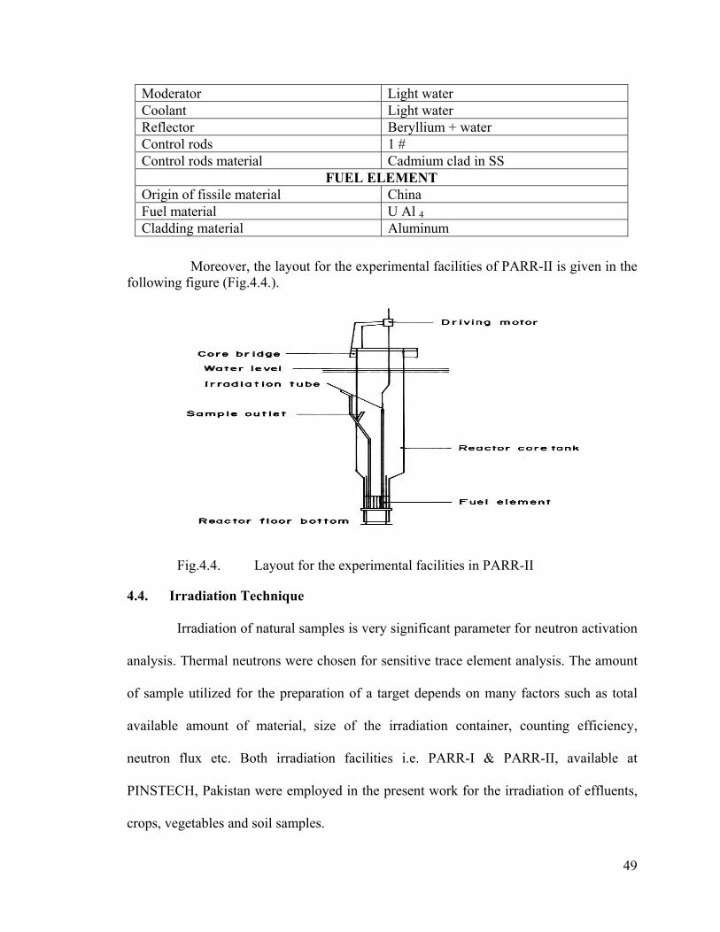
49
Moderator Light water Coolant Light water Reflector Beryllium + water Control rods 1 # Control rods material Cadmium clad in SS
FUEL ELEMENT Origin of fissile material China Fuel material U Al 4 Cladding material Aluminum
Moreover, the layout for the experimental facilities of PARR-II is given in the following figure (Fig.4.4.).
Fig.4.4. Layout for the experimental facilities in PARR-II
4.4. Irradiation Technique
Irradiation of natural samples is very significant parameter for neutron activation
analysis. Thermal neutrons were chosen for sensitive trace element analysis. The amount
of sample utilized for the preparation of a target depends on many factors such as total
available amount of material, size of the irradiation container, counting efficiency,
neutron flux etc. Both irradiation facilities i.e. PARR-I & PARR-II, available at
PINSTECH, Pakistan were employed in the present work for the irradiation of effluents,
crops, vegetables and soil samples.

50
4.4.1. Container/ Rabbit for Irradiation
Rabbit and containers were utilized in order to segregate the sample material from
external turbulence and to protect the reactor pool from contaminations in case of any
breakage/ spillage of the sample materials. Irradiation containers for long irradiations
were prepared from aluminum material and had low contents of sodium, manganese and
copper as impurities. Irradiation capsules and rabbits employed for all other modes of
irradiations were made of polyethylene. The size of such capsule was 1.5 x 1.0 cm2 while
for rabbit; it was 3.0 x 6.6 cm2. The capsules were pretreated for decontamination from
grease and other materials by extensive washing with fresh tap water, dilute (about 02
molar) HNO3 solution and then with distilled/ demineralized water (DMW). After
washing, they were dried in an oven at 80 C for about 24 hours. Empty ampoules were
weighed and were affixed proper number/ code on the top & side of each ampoule.
4.4.2. Calculations for measurement of radioactivity
Determination of radioactivity for all concerned elements was a fundamental
requirement, before irradiation of samples with PARR-I or PARR-II, to avoid any
accident during irradiation. The following formula was applied for the calculation of
activity measurements.
iWNawA e T
it
2/1
693.0
1
A Activity in Bq (3.7 x 10⁷ Bq 1m Ci)
w Weight of sample taken (in gm)
a Abundance of natural element (%)
σ Neutron cross section of isotope in barns (1 barn 10–24 cm2)

51
Wi Atomic weight of isotope prepared (in gm)
ti Time of irradiation of element (in seconds)
T1/2 Half life of isotope (in seconds)
N Avogadro # 6.023 x 10²³
φ Neutron flux in Reactor (1014 n. cm2 s-1)
By inserting the values of different common factors, the final shape of
the formula becomes as follow where the unit for Activity is in mCi & Neutron cross
section of isotope is in Cm2.
610628.11 2/1
693.0
iWawA e T
it
(1)
1.628 x 10⁶ 10–24 x 1014 x 6.023 x 1023 / 3.7 x 10⁷
The nuclear data [128], which was applied for the computation of radioactivity of
the elements in the samples, before the irradiation of samples through PARR-1 or PARR-
II, is shown in the Table 4.9.
Table: 4.9 Nuclear data, essential to calculate the activity of the elements for irradiation [128]
Element Abundance (a %)
Neutron Cross section (б)
Isotope used
Half life (T1/2)
Irradiation time (t)
27Al 100.0 0.23 28Al 2.264 m 02 m 48 Ca 0.19 1.1 49 Ca 8.72 d 02 m 65 Cu 30.9 2.17 66 Cu 5.1 m 02 m 26 Mg 11.01 0.038 27 Mg 9.46 m 02 m 50 Ti 5.3 0.179 51 Ti 5.8 m 02 m 51 V 99.75 4.88 52 V 3.75 m 02 m 37 Cl 24 0.433 38 Cl 37.18 m 05 m 55 Mn 100.0 13.3 56 Mn 2.6 h 10 m 75 As 100.0 4.3 76 As 26.4 h 25 m

52
41 K 006.7 1.46 42 K 12.36 h 35 m 139 La 099.9 9.0 140 La 40.3 h 35 m 23 Na 100.0 0.4 + 0.13 24 Na 15.0 h 35 m 130 Ba 000.1 2.5 + 11 131 Ba 11.5 d 300 m 140 Ce 088.5 0.57 141 Ce 32.51 d 300 m 59 Co 100.0 20 + 17 60 Co 5.272 y 300 m 50 Cr 004.35 15.9 51 Cr 27.7 d 300 m 133 Cs 100.0 2.5 + 26.5 134 Cs 2.06 y 300 m 151 Eu 047.8 4.0 + 3300 + 5900 152 Eu 12.4 y 300 m 58 Fe 000.28 1.3 59 Fe 44.6 d 300 m 180 Hf 035.1 12.6 181 Hf 42.4 d 300 m 202 Hg 029.7 4.9 203 Hg 46.6 d 300 m 176 Lu 100.0 2050 177 Lu 6.7 d 300 m 85 Rb 072.17 0.05 + 0.41 86 Rb 18.7 d 300 m 121 Sb 057.3 0.055 + 6.2 122 Sb 2.7 d 300 m 45 Sc 100.0 9.6 + 16.9 46 Sc 84 d 300 m 74 Se 000.9 51.8 75 Se 120 d 300 m 154 Sm 022.5 5.5 155 Sm 23.5 m 300 m 181 Ta 099.9 0.0103 + 21.0 182 Ta 115 d 300 m 159 Tb 100.0 25.5 160 Tb 72 d 300 m 232 Th 100.0 7.4 233 Pa 27.d 300 m 168 Yb 00.14 3470 169 Yb 30.7 d 300 m 64 Zn 48.9 0.78 65 Zn 244 d 300 m 94 Zr 17.5 0.056 95 Zr 64.0 d 300 m
4.4.3. Protocol for Sample Irradiation
The irradiation method was the most significant in calculating the quality of the
product obtained [129]. The aim of irradiation was to produce sufficient activity in the
sample, taking into account the decay time to analyze the gamma spectrum. Preparation
of all the samples for neutron irradiation was performed under standard terms and
conditions. Safety measures were adopted to avoid any cross contamination. In the
laboratory, all the samples were processed in Laminar flow fume hood (Kotterman 8580).

53
The working tables were protected with clean Polyethylene sheets. After wearing lab coat
and Polyethylene disposable gloves, all the samples were processed. For irradiation 100-
125 mg dry weight powder of geological (soil)/ effluent samples and 200-250 mg dry
weight powder of vegetable/ crop samples was used for each sample. The corresponding
standard reference materials, for each sample, were also packed and sealed in the pre-
cleaned ampoules for simultaneous irradiations. Same weight of the sample and standard
materials were used to avoid the errors from self- absorption of the neutron flux. All
ampoules were arranged in the form of stacks in rabbit, as given in Fig. 4.5.
Fig. 4.5 Stack arrangements of sample ampoules in Rabbit for irradiation at reactors
Samples irradiation for long, intermediate and short time interval was performed
for 300, 10 – 35 and 02 minutes respectively. All the samples were irradiated for long,
intermediate and short times at PARR-I and PARR-II, according to the approved standard
irradiation procedures/ protocols.

54
4.5. Gamma - Spectrometric Instrumentation [130]
Gamma spectrometric instrumental set-up was applied for the studies of the
elemental analysis of effluents, crops, vegetables and soil samples for the estimation of
polluted ecosystem caused by the industrial pollution. The instrumental setup consists of
a high purity germanium detector, ORTEC Co-axial HPGe, which was attached to a PC-
based multi-channel analyzer (MCA Inter- Technique model pro – 286e) through a
sensitive spectroscopy amplifier (CANBERRA model 2022). The detector is operated at
liquid nitrogen temperature (77 K) and the crystal is mounted in a vacuum cryostat. The
software “Inter-gamma, version 5.03” was utilized for the measurements. The resolution
of the system is 1.9 keV for 1332.5 keV peaks of 60Co along with a peak to Compton ratio
of 40:1. This is the ratio for the evaluation of the detector’s capability to differentiate low-
energy peaks in the presence of high-energy sources. The data from MCA was then
shifted to the personnel computer for processing and statistical analysis of the results.
Complete setup for gamma spectrometry is presented as a block diagram in Fig.4.6.
Fig. 4.6 Block diagram for a gamma spectroscopy system

55
4.5.1. Description of Instruments for NAA
There is a series of different instruments in the gamma spectroscopy. NaI(Th),
Si (Li), Ge (Li) etc detectors are normally utilized for the detection of Gamma rays. In the
present research, the High Purity Germanium (HPGe) detector was used. The detector can
resolve two gamma rays with an energy difference of 3-6 KeV only. The limitations of
HPGe detectors are their high cost and the continuous need to be cooled with liquid
nitrogen to avoid re-diffusion of the Lithium and to minimize electronic noise. Moreover,
other significant instruments are detector bias high voltage supply, Pulser, Pre-amplifier,
Spectroscopic amplifier, Multi-Channel Analyzer (MCA), Integral Discriminator,
Differential Discriminator (SCA), Computer, Printer etc.
4.5.2. Calibration of the Detectors for NAA
Schedule checkup for channel energy calibration of the detector with two point
sources 152Eu and 60Co was executed. 152Eu source was placed on detectors at a height of
10 cm above the top of the detector. Spectrum was achieved for 100 seconds. Energy
channels for the major peaks i.e. 121.8, 244.7, 344.3, 411.1, 444, 778.9, 867.4, 964,
1085.8, 1112, 1408.1 keV were used. Subsequently same procedure was repeated with
60Co source of its two main peaks at energy channels 1173.2 and 1332.5 keV. By using
these two sources, especially for lower energy spectrum, the MCA was calibrated. For the
present research, the resolution of the system was 1.9 keV for 1332.5 keV gamma-peaks
of 60Co and peak/ Compton ratio was 70:1.
4.5.3. Essential parameters for the Gamma Spectrometry
Following essential parameters were observed during the Gamma spectrometric
analysis to obtain the best results within 5% accuracy as presented in the Table 4.10.

56
Table 4.10 Operating conditions for the Gamma spectrometric analysis
Sr. No.
Parameters Descriptions
1. Weight of Soil Sample taken 0.025 mg to 0.05 mg
2. Weight of Bio Sample taken 0.1 mg to 0.15 mg
3. Nature & composition of the Standard material Similar with the sample
4. Weight of the Standard Material taken Equivalent to sample’s Wt.
5. Nuclear Reactor Power 9MW – 10 MW
6. Thermal Neutron Flux Density 7 x 10¹³ n. cm-2 sec-1
7. Energy of Thermal Neutrons 0.025 eV at 25 °C
8. Possible Irradiation Reaction (n, ) reaction
9. Position of Sample & Standard in Reactor core As close as possible
10. Dead time for sample analysis 0 – 5%
11. Full Width with Half Maximum (FWHM) 1.2 keV for 122 keV -rays to 2.1 keV for 1332.5 keV -rays
12. Counts under the area of the Gamma Peak 100 – 10,000 Counts
4.5.4. Gamma scanning of the radionuclides
The gamma scanning of particular radionuclides was executed by applying
standard recommended procedure. During the scrutining of the samples, which were
irradiated for 05 to 10 minutes, only 04 elements were detected. The nuclear data and
essential parameters for this category are presented in Table 4.11.
Table 4.11 Nuclear data of intermediate term irradiation conditions (05 to 10 min) for effluents, crops, vegetables and soil samples at PARR-1
Elements for search
Radionuclides formed
Half life (T1/2)
-Ray used (KeV)
Irradiation Time
Cooling Period
Counting Time
37Cl 38Cl 0.62 h 1642 05 to 10 minutes
04 to 26 hours
02 to 15 minutes 55Mn 56Mn 2.57 h 847
41K 42K 12.3 h 1525 23Na 24Na 15.0 h 1369

57
Five elements were calculated during gamma scanning of those samples, which
were irradiated for 25 to 35 minutes. Prescribed cooling time was allotted to a particular
sample for decay of the undesired elements, prior to its analysis. The essential parameters
for this category are listed in Table 4.12.
Table 4.12 Nuclear data of intermediate term irradiation conditions (25 to 35 min) for effluents, crops, vegetables and soil samples at PARR-1
Elements for search
Radionuclides formed
Half life (T1/2)
-Ray used (KeV)
Irradiation Time
Cooling Period
Counting Time
75As 76As 26.30 h 559 25 to 35 minutes
02 to 06 days
10 to 25 minutes 81Br 82Br 35.40 h 554, 777
139La 140La 40.30 h 486, 1596 41K 42K 12.40 h 1525 23Na 24Na 15.00 h 1369
Long-term irradiation of samples was conducted for 300 minutes. During gamma
spectrometry, precise peaks of twenty elements were obtained. The essential parameters
used for 300-minute irradiation of samples are presented in Table 4.13.
Table 4.13 Nuclear data of long-term irradiation conditions (300 min) for effluents, crops, vegetables and soil samples at PARR-1
Elements for search
Radionuclides formed
Half life (T1/2)
-Ray used (KeV)
Irradiation Time
Cooling Period
Counting Time
130Ba 131Ba 11.50 d 496 05 to 12 hours
04 to 06 weeks
03 to 30 hours 140Ce 141Ce 32.40 d 145
59Co 60Co 05.26 a 1173, 1332 50Cr 51Cr 27.80 d 320 133Cs 134Cs 02.00 a 604, 796 151Eu 152Eu 12.70 a 1408 58Fe 59Fe 44.60 d 1099, 1291 180Hf 181Hf 42.50 d 133, 482 85Rb 86Rb 18.60 d 1078 123Sb 124Sb 60.20 d 1691 45Sc 46Sc 83.90 d 889, 1120 74Se 75Se 120.0 d 264, 279 153Sm 154Sm 46.60 h 103

58
84Sr 85Sr 64.50 d 513 181Ta 182Ta 115.0 d 1188, 1221 159Tb 160Tb 72.10 d 298, 879 232Th 233Th 27.4 d 311 168Yb 169Yb 31.80 d 177, 198 64Zn 65Zn 243.8 d 1115 94Zr 95Zr 65.50 d 724, 756
Irradiation for 02 minutes at PARR-II was carried out for sequential analysis.
During gamma spectrometry, distinct peaks of ten elements were characterized. For this
category used irradiation, cooling and counting parameters are shown in the Table 4.14.
Table: 4.14 Nuclear data of short-term irradiation conditions (02 minutes) for effluents, crops, vegetables and soil samples at PARR-II
Elements for search
Radionuclides formed
Half life (T1/2)
-Ray used (KeV)
Irradiation Time
Cooling Period
Counting Time
27Al 28Al 02.25 m 1779 02 minute 03 to 06 minute
02 to 05 minute 48Ca 49Ca 08.72 m 3084
37Cl 38Cl 37.30 m 2167 65Cu 66Cu 05.10 m 1039 41K 42K 738.0 m 1525 26Mg 27Mg 09.50 m 843 55Mn 56Mn 155.0 m 847 23Na 24Na 900.0 m 1369 50Ti 51Ti 05.80 m 320 51V 52V 03.75 m 1434
4.6. Statistical Calculations
For the calculation of elemental concentrations, in each sample of effluents,
soils, crops and vegetables, the following parameters were encountered.
4.6.1. Correction with back ground counts
To achieve the best results, all possible sources of error were considered. Decay
factor and other correction factors were also employed to enhance the efficiency and
accuracy. The Background correction was calculated by utilizing the following formula:

59
C U A P Bg X C T Samp
C U A P Samp (Corrected) = C U A P Samp – -------------------------------------
C T Bg
Where, C U A P Samp (Corrected) Counts Under the Area of Peak of Sample, after background
correction
C U A P Samp Counts Under the Area of Peak of Sample
C U A P Bg Counts Under the Area of Peak of Back ground
C T Samp Counting Time of Sample
C T Bg Counting Time of Back ground 4.6.2. Decay Factor
The decay factor was utilized for the normalization of the time delay of sample as
compared to the analysis time of the standard.
Decay Factor
21T
t693.0e
Where: t time difference between standard and sample analyses T1/2 Half life of a radionuclide
Formula with “▬” value predicted that the sample was analyzed before the
standard. Formula with “+” value indicated that the standard was analyzed before the
sample. Results were within the range of 5% for accuracy.
4.6.3. Concentration of elements
Neutron activation counting of samples produced gamma spectra, which
indicated sharp peaks for each element. More than 30 elements in each sample were
recognized due to the characteristic energy of each peak. By applying the following
formula, the calculation of the concentration of each element was done by incorporating
the counts under the area of a specific peak along with other parameters.

60
CUAP Samp X Wt Std X CT Std X CV X Decay Factor
Conc = -------------------------------------------------------------------- CUAP Std X Wt Samp X C T Samp
Where:
Conc Concentration of desired element in the sample (units in ppm or %)
C T Std Counting Time of Standard
C T Samp Counting Time of Sample
C V Certified Value of a standard element from literature/ catalogue of standard
C U A P Std Counts Under the Area of Peak of standard
C U A P Samp Counts Under the Area of Peak of Sample
Wt Std Weight of Standard
Wt Samp Weight of Sample
4.7. Preparation of solutions for AAS analysis
Atomic absorption spectrometric (AAS) sample analysis was a comparative
technique. All sort of samples were analyzed in the form of solutions. For the analysis of
crop, vegetable, soil and effluent samples, a variety of solutions were prepared such as
standard solution, reference blank solutions, IAEA reference material solutions etc. To
reduce the errors in the results, all the reagents used were of Analar grade. Distilled water
and demineralized water (DMW) were consumed for the preparation of the solutions. All
glasswares utilized were cleaned by over night soaking them in dilute Nitric acid
followed by multiple rinses with tap water and then dried in oven. The following different
kinds of solutions were prepared for the analysis of the samples.
4.7.1. Stock solutions
Each stock solution contained a concentration of 1000 ppm for concerned
element/ metal. Commercially available stock solutions of Co, Cd, Ni, Pb, Fe, Cu, Mn
and Zn elements were used for all analysis through AAS.

61
4.7.2. Standard blank solution
For the preparation of dilute nitric acid (01 molar concentration with a volume of
01 liter) solution, as a standard blank solution, 65 ml of concentrated HNO3 were mixed
with 935 ml distilled water in a measuring flask. This solution was utilized for the
dilution of stock solutions.
4.7.3. Standard solutions
Standard solutions were prepared by diluting the stock solution of concerned
element, with standard blank solution, just before their analysis. Such diluted acidic
solutions of each required element, contained different concentrations e.g. 1, 2, 3, 4, & 5
ppm, according to the requirement of the analysis.
4.7.4. Solutions of geological and effluent samples
Soil, IAEA reference material and effluent dry samples were converted in to
solution form by the prescribed recommended procedure. 0.5 gram IAEA-S-7 dry sample
or dry effluent sample was taken in a teflon beaker and 10 ml Aquaregia (3 ml conc. HCl
: 1 ml conc. HNO3) was mixed with it. The mixture was dried on a hotplate at 80 ºC.
Filtrate and precipitates were separated through filtration technique. 5 ml conc. HF and 1
ml conc. H2SO4 were added in the residue. Heating and fuming were done for two times.
Then 1 ml conc. HF, 0.5 ml conc. HClO4, 0.5 ml conc. H2SO4 and 2 ml Aquaregia were
added in it. Heating was done up to fuming. Again 5 ml Aquaregia was added and filtrate
was also mixed. The final volume was made up to 50 ml with DMW.

62
4.7.5. Blank solution for geological and effluent samples
10 ml Aquaregia was used in a teflon beaker and 1 ml conc. H2SO4 with 5 ml conc.
HF were mixed. After dryness, 1 ml conc. HF, 0.5 ml conc. HClO4, 0.5 ml conc. H2SO4
and 7 ml Aquaregia were added. Finally, the volume was made up to 25 ml with DMW.
4.7.6. Solutions of crop and vegetable samples
Dry samples of crop and vegetable were converted in to solution forms by
adapting the following procedure. In a tephlon bomb, 0.5 gram dry sample was mixed
with 5 ml conc. HNO3 and 1 ml conc. H2O2. The mixture was placed in a Micro-wave
oven for 35 minutes to dissolve the sample at high pressure and temperature. After
required time to cool the bomb, the sample was extracted in a tephlon beaker and it was
dried on a hot plate at 100 ºC. Then the dried treated sample was mixed with 1 ml conc.
H2SO4, 1 ml conc. HClO4, 0.5 ml conc. H2O2, 2 ml Aquaregia and 0.5 ml conc. HF. The
mixture was again dried up to fuming. 5 ml reverse Aquaregia (3 ml conc. HNO3 : 1 ml
conc. HCl) and 1 ml distilled water were mixed and again it was heated to dryness. After
cooling, the volume was made up to 25 ml with DMW.
4.7.7. Blank solution for crop and vegetable samples
5 ml conc. HNO3 was taken in a tephlon beaker with 1 ml conc. H2O2. The
solution was heated on a hot plate up to dryness. Then 1 ml conc. H2SO4, 1 ml conc.
HClO4, 0.5 ml conc. H2O2, 2 ml Aquaregia and 0.5 ml conc. HF were mixed with it. After
complete dryness, the precipitate was dissolved in 5 ml reverse Aquaregia (3 ml conc.
HNO3: 1 ml conc. HCl). Finally, the volume was made up to 25 ml with DMW.

63
4.8. Analysis of samples through Atomic Absorption Spectrometry (AAS)
Atomic Absorption Spectrometry (AAS) was a susceptible means for the
qualitative and quantitative measurement of more than 60 metals/ elements. For the
analysis of effluents (from ceramics, paper and textile industries), soils (from upper and
lower surfaces of Faisalabad and Gujranwala industrial areas), crops (i.e. wheat, rice and
maize), vegetables (i.e. cabbage and tomato) and IAEA standard material (i.e. S-7)
samples, all relevant solutions were prepared according to the literature cited procedures.
The analysis was carried out using a Hitachi model Zeeman-8000, Atomic absorption
spectrometer with a polarized Zeeman’ effect and background correction mode. The
spectrometer was equipped with a graphite furnace, a microprocessor based data handling
facility and an auto-sampler. A water cooled, premix, fishtail type burner, heaving 10 x
0.05 cm2 size, was employed for the air-acetylene flame. Hollow cathode lamps of each
metal i.e. chromium, cobalt, cadmium etc., from Hitachi were used as radiation sources
for each respective metal. The measurements were made employing electro-thermal
atomization technique. Calibration curves (for sample and standard solutions) were
obtained under identical conditions by extracting the concentration of required metal. By
taking measurements for triplicate runs, the reproducibility of the obtained data was
checked. The precision achieved was better than ±1.5 %. The instrumental response was
documented at a high S/N ratio (Signal to Noise ratio = S/N = Mean/ Standard deviation
= X / δ). Moreover, the detection limit for flame AAS was within the range of ±0.2 to
±30 ng/ ml. The accuracy range was ±0.5 % to ±1.0%. To reduce the errors in the results,
a suitable slit width, for each element, was chosen because a broad slit width degraded its
sensitivity and aggravated curvature of calibration curves.

64
4.8.1. Atomic Absorption Spectrometric Instrumentation
Hitachi Atomic Absorption Spectrometer model Z-8000, with a Zeeman-effect/
background correction mode, was employed for all measurements. It comprises of a
graphite furnace, an auto-sampler and a computer based programme for sample analysis.
Argon was consumed as an inert purging gas; the flow was interrupted during the
atomization step. Signal assessment was based on integrated absorbance values. The
measurements of cadmium (Cd), cobalt (Co), copper (Cu), iron (Fe), manganese (Mn),
nickel (Ni), lead (Pb) and zinc (Zn) were processed with an electro-thermal atomization
technique. A complete system for sample analysis through the atomic absorption
spectrometric technique is shown as a block diagram in Fig. 4.7.
Fig. 4.7 Block diagram for Atomic Absorption Spectrometry 4.8.2. Analytical parameters for AAS analysis
The selection of optimum conditions was crucial to obtain high sensitivity in
practical analysis. The atomic absorption spectrometric technique involved a number of
operating parameters based on atomization mode and instrumental optical design. Air-
Acetylene flame was utilized for atomization of all selected elements. Other optimum
parameters, which were used for AAS analysis, are shown in Table 4.15.

65
Table 4.15 Analytical parameters for AAS analysis [131]
Metal Resonance Absorbance line λ (nm)
Interfering agents
Instrument detection limit (μg/ml)
Sensitivity (μg/ml)
Optimum concentration range (ppm)
Cadmium (Cd)
228.8 Silicon 0.002 0.025 0.05 – 6.0
Copper (Cu)
324.8 NIL 0.01 0.1 0.2 – 30
Iron (Fe)
248.3 Silicon 0.02 0.12 0.3 – 20
Manganese (Mn)
279.5 Molybdenum & Silicon
0.01 0.05 0.1 – 20
Nickel (Ni)
232.0 NIL 0.02 0.15 0.3 – 10
Lead (Pb)
217.0 Aluminum & Silicon
0.05 0.5 1.0 – 200
Cobalt (Co)
240.7 Aluminum & Calcium
0.03 0.2 0.5 – 10
Zinc (Zn)
213.8 Silicon 0.005 0.02 0.05 – 4.0
4.8.3. Instrumental operating conditions and specifications
The analysis was executed for all concerned elements, by the alteration of
instrumental conditions at optimum levels such as utilized Burner was standard type,
Oxidant was Air at a pressure of 1.6 Kg/cm2, Measurement mode was direct, Analytical
mode was concentration (ppm) and the Equation type was linear fit. Other selected
instrumental operating conditions and specifications are illustrated in Table 4.16.
Table 4.16 Instrumental operating conditions and specifications for AAS [131]
Metal Lamp current (mA)
Width of Slit (Cm)
Burner height (Cm)
Fuel & flow-rate (L/mim)
Cadmium (Cd)
7.5 1.3 7.5 C2H2 2.2
Cobalt (Co)
12.5 0.2 10.0 C2H2 2.5
Copper 7.5 1.3 7.5 C2H2

66
(Cu) 2.3 Iron (Fe)
12.5 0.2 7.5 C2H2 2.3
Manganese (Mn)
7.5 0.4 7.5 C2H2 2.3
Nickel (Ni)
12.5 0.2 7.5 C2H2 2.3
Lead (Pb)
7.5 1.3 7.5 C2H2 2.3
Zinc (Zn)
10.0 1.3 7.5 C2H2 2.0
4.9. Sources of errors
Reliability, reproducibility and accuracy are the fundamentals of analytical
chemistry. Precision, standard deviation of measurements and absolute/ relative errors are
the significant parameters for an analyst to produce an authentic data. The instrumental
errors, method errors, operational errors, personal or human errors and determinate errors
are the major sources of error for any measurement. To ensure the validity and integrity
of the results, all possible sources of error are identified and reduced. In this research
work, the possible sources of errors [17] for NAA were weighing, dead time (5%), peak
area measurements, full width with half maximum (FWHM optimum range 1.2 – 2.1),
peak’s back ground correction, efficiency of detection, spectrum size, counting time,
neutron flux, absolute decay rate, position in the reactor for irradiation, uncertainties in
the number of target nuclei ( 1%) as well as in irradiation and cooling times (1%). To
minimize the errors, representative and un-contaminated samples were used. Neutron
activation/ atomic spectro-metric measurements and spectra analysis were performed
carefully. All results were quoted with 95% confidence level and overall error was within
1% accuracy.
67
CHAPTER-5
5. RESULTS (Evaluation of trace elements)
For the evaluation of trace elements, the samples of vegetables, crops, soil and
industrial effluents were analyzed through Neutron Activation Analysis (NAA) and
Atomic Absorption Spectrometric (AAS) techniques. The scientific, common, vernacular,
family and English names to which each vegetable/ crop belonged, are given in Table 4.1
(section 4.1.1). Their elemental concentrations were calculated on dry weight basis and
each mean value was an average of at least six or more individual measurements along
with their standard deviations. In each sample, thirty major, minor and trace elements
including essential, non-essential, toxic and rare earth elements were determined. The
data obtained is expressed here in the tables 6.1 to 6.12. Due to their significance, all the
results are classified in the following eight categories.
5.1. Validation of methodology for NAA technique
The analysis of Certified Reference Materials (CRMs) were executed for the
quality assurance measures of the analytical data in order to minimize the measurement
errors to the reasonable limits and the results were cited within a confidence limit of 95%.
A comparison for elemental concentrations (g/g) shows that the results of present work
are in good agreement with the cited values of the CRMs within 1 error. The details of
geological and biological CRMs, along with their trace elements, utilized for this work,
are given in Table 4.5 (section 4.2). The results obtained from this work and the certified/
cited values for concentrations of trace elements for all employed CRMs i.e. Lichen, CL,
WP, SL-1 and S-7 are presented in Table 5.1.

68
Table 5.1 Comparison of the trace elemental concentrations (g/g) for reference values of biological (Lichen, Citrus Leaves & Whey Powder) and geological (SL-1 & S-7) Standard Reference Materials (SRMs) with present work analyzed through NAA technique
Elements IAEA-336 Lichen
NBS/ SRM-1572 Citrus Leaves (CL)
IAEA-155 Whey Powder (WP)
IAEA/ SL-1 (Lake Sediment)
IAEA/ S-7 (Soil)
Reference Values
Present work
Reference Values
Present work
Reference Values
Present work
Reference Values
Present work
Reference Values
Present work
As 0.63 0.39±0.12 03.10 2.79±0.16 0.049 0.09±0.019 27.5 32±2.25 13.4 11.5±0.95 Ba 6.40 4.7±0.85 21.0 32.69±5.85 NC ND 639.0 654±7.5 159.0 155±2.0 Br 12.9 13.6±0.35 8.20 6.82±0.69 39.1 37.1±1.0 6.82 6.5±0.16 7.0 8.8±0.9 Ca NC ND 31500.0 33752±1126 42100.0 42218±59 2500.0 2473±13 163000.0 162136±432 Ce 1.28 1.58±0.15 0.28 0.42±0.07 NC ND 117.0 113.8±1.7 61.0 66±2.5 Cl 1900.0 1926±13.0 414.0 386.9±63 69200.0 65780±1710 10.0 14.7±2.35 NC ND Co 0.29 0.22±0.03 0.02 0.03±0.005 0.043 0.056±0.007 19.8 19.4±0.2 8.9 9.1±0.1 Cr 1.06 1.36±0.15 0.80 1.06±0.13 0.59 0.63±0.02 104.0 105.7±0.85 60.0 59.38±0.3 Cs 0.11 0.16±0.02 0.098 0.101±0.03 0.086 0.076±0.005 7.01 6.4±0.3 5.4 5.32±0.04 Cu 3.60 3.2±0.2 16.50 16.1±0.2 0.57 0.42±0.07 30.0 25.7±2.1 11.0 12.85±0.9 Eu 0.023 0.039±0.018 0.01 0.02±0.01 NC ND 1.6 1.98±0.19 1.0 0.98±0.01 Fe 430.0 426±2.0 90.0 116±28 62.0 67.7±2.85 67400.0 67274±63 25700.0 25820±60 Hf NC ND NC ND NC ND 4.16 4.48±0.16 5.1 4.74±0.18 K 1840.0 1769±35.5 18200.0 17384±408 41700.0 40986±357 15000.0 14825±587 12100.0 12386±143 La 0.66 0.55±0.05 0.19 0.21±0.01 NC ND 52.6 54.4±0.9 28.0 26.8±0.6 Mg NC ND 5800.0 5768±16 3190.0 3218±14 29000.0 28682±159 11300.0 11698±199 Mn 63.0 58.6±2.2 23.0 22.32±0.34 9.3 9.99±0.34 3460.0 3566±53 631.0 665.6±17 Na 320.0 333±6.5 160.0 146.4±16.8 15800.0 15692±304 1720.0 1685±37 2400.0 2511±55 Rb 1.76 1.28±0.24 4.84 4.57±0.13 39.2 45.8±7.3 113.0 119±3.0 51.0 53.89±1.45 Sb 0.073 0.087±0.007 0.04 0.31±0.03 NC ND 1.31 1.51±0.1 1.7 1.49±0.1 Sc 0.17 0.19±0.01 0.01 0.02±0.01 0.028 0.024±0.002 17.3 16.81±0.25 8.3 8.54±0.12 Se 0.22 0.27±0.02 0.025 0.031±0.003 0.064 0.051±0.006 2.9 2.58±0.16 0.4 0.52±0.06 Yb 0.037 0.042±0.008 NC ND NC ND 3.42 3.65±0.1 2.4 2.22±0.09 Zn 30.4 35.3±2.55 29.0 33.1±5.05 34.3 29.5±2.4 223.0 254±15 104.0 97.28±3.3

69
5.2. Validation of methodology for AAS technique
All the samples, for the present work, were analyzed mainly through neutron
activation analyses (NAA) technique. However, for the verification of the obtained
results, atomic absorption spectrometric (AAS) technique was also employed for
quantitative evaluation of selected samples of crops, vegetables, soil and effluents. In this
regard, the dissolution of soil samples was very significant process that is illustrated in
the section 4.7.4. For the validation of this technique, Table 5.2 presents the comparison
about the results (μg/g) of trace elements analyzed through AAS technique for IAEA
standard reference materials Lake sediment (SL – 1) and Soil (S – 7) with present work
along with its Standard Deviations (SD).
Table 5.2 Comparison of the trace elemental concentrations (g/g) for reference values of IAEA Standard Reference Materials (SRMs) with present work analyzed through AAS technique
Elements IAEA/ SL-1 (Lake Sediment)
IAEA/ S-7 (Soil)
Reference Values
Present work
Reference Values
Present work
As 27.5 ND 13.4 ND Cd 1.3 1.02±0.6 1.3 1.08±0.71 Co 19.8 20.3±1.4 8.9 9.82±0.92 Cr 104.0 107±4.8 60.0 63.2±2.60 Cu 30.0 28.1±3.2 11.0 12.38±1.20 Fe 67400.0 66928±81 25700.0 26130±215 Mn 3460.0 3569±72 631.0 623±21 Ni 26.0 27.3±1.7 26.0 29±1.50 Pb 60.0 61.8±0.8 60.0 63.8±1.90 Sb 1.31 ND 1.7 ND Se 2.9 ND 0.4 ND Zn 223.0 242±21 104.0 112.58±9.29

70
5.3. Trace elemental contents in the Effluents
The effluents, engaged for the cultivation purposes, were collected from textile,
pulp and ceramics industries periodically. They were analyzed for pollution parameters
(chemical analysis) and trace elemental concentrations (soluble ions) through NAA and
AAS techniques. More than 100 samples of effluents from a variety of industries were
collected and analyzed for the present study. The concentrations (g/l) of trace elements
in the industrial effluents of textile/ yarn, pulp/ paper and ceramics are shown in Tables
5.3.a, b & c respectively. While the chemical analysis of industrial effluents of textile/
yarn, pulp/ paper & ceramics, collected from industries of Faisalabad and Gujranwala, is
presented in Tables 5.4.a, b & c respectively.

71
Table 5.3.a Concentrations (g/l) of trace elements in the effluents of textile/ yarn industry
Industry Codes/ Elements
T-503 T-510 T-520 T-529 T-544 T-549
As 26.7±0.6 15.2±1.0 49.1±1.8 21.7±1.2 37.9±2.6 29.9±1.7
Ba 220±14.3 156±38.7 130±19.0 139±14.7 224±15.5 178±12.3
Br 67.3±0.1 52.4±1.6 59±1.6 56±1.2 75±2.1 45±2.6
Ca 15917±143 12513±185 17760±130 12367±240 19247±142 14765±108
Cd 0.93±0.06 1.05±0.07 1.21±0.08 0.86±0.06 0.99±0.07 1.11±0.09
Ce 10.3±1.0 17.6±1.7 18.3±2.0 16.7±1.8 17.8±1.7 18.6±1.6
Cl 15120±115 19100±144 12430±194 16446±148 18388±163 14271±192
Co 5.51±0.19 8.5±0.3 2.2±0.2 7.48±0.81 7.29±0.23 6.5±0.24
Cr 4.84±0.28 4.3±0.2 9.49±0.6 8.5±0.5 8.4±0.5 8.25±0.21
Cs 4.5±0.4 4.4±0.1 3.6±0.42 3.8±0.04 3.3±0.05 2.45±0.12
Cu 37.43±1.06 37.66±1.07 38.01±1.05 34.3±2.08 21.90±2.1 32.7±1.51
Eu 0.2±0.01 0.3±0.02 0.35±0.03 0.4±0.05 0.5±0.04 0.21±0.09
Fe 9224±80 8773±57 9350±87 7344±44 7586±53 8807±84
Hf 0.46±0.05 0.86±0.09 0.24±0.02 0.9±0.09 0.7±0.01 0.4±0.04
K 24315±896 13046±326 18380±460 18744±474 18703±688 21574±616
La 0.12±0.03 0.6±0.01 0.13±0.03 0.23±0.01 0.15±0.04 0.31±0.08
Mg 5219±147 5918±164 5868±159 6525±268 7432±306 6217±271
Mn 25.2±1.0 34.8±0.5 53.7±1.4 39.4±0.5 30±0.4 51.1±0.7
Na 15791±546 16220±706 24031±512 15904±657 12893±495 14284±456
Ni 33±3.1 29±1.7 36±2.3 40.1±3.3 22.8±1.1 25.6±1.6
Pb 52±4.6 46±3.4 55±4.8 42±3.1 58±4.8 49±4.1
Rb 0.79±0.07 0.64±0.02 0.56±0.04 0.88±0.05 0.69±0.06 0.98±0.08
Sb 1.41±0.03 1.24±0.05 1.59±0.01 1.89±0.04 1.79±0.03 1.63±0.03
Sc 1.45±0.23 1.04±0.17 1.5±0.5 1.64±0.26 2.48±0.39 1.48±0.4
Se 0.4±0.01 0.39±0.01 0.32±0.03 0.11±0.01 0.1±0.01 0.48±0.01
Yb 0.19±0.02 0.16±0.05 0.2±0.05 0.23±0.06 0.25±0.04 0.29±0.02
Zn 79.2±0.2 70.8±0.3 45.3±1.1 62.0±1.5 75.5±1.9 74.5±1.9

72
Table 5.3.b Concentrations (g/l) of trace elements in the effluents of pulp/ paper/ board industry
Industry Codes/ Elements
P-312 P-313 P-320 P-324 P-335 P-338
As 25±1.3 24±2.1 20±0.5 15.1±4.4 26±7.4 15.4±4.4
Br 37±4.9 42±1.8 18.3±3.2 43±7.5 33±2.1 40±5.7
Ca 22980±692 21360±547 29786±897 23267±605 24665±733 9054±585
Cd 0.47±0.02 0.51±0.03 0.57±0.03 0.42±0.01 0.49±0.02 0.54±0.04
Ce 24±0.1 25.7±1.4 16±0.1 15.1±1.0 24.3±1.4 18.7±1.1
Cl 18450±501 19815±744 15428±692 6475±504 12179±232 19062±687
Co 4.1±0.8 2.45±0.1 3.1±0.6 1.6±0.2 2.7±0.3 1.7±0.2
Cr 31.17±1.67 35.4±1.1 25.87±1.88 21.92±1.28 24.2±1.1 36.5±1.5
Cs 1.8±0.01 1.1±0.1 1.5±0.01 1.56±0.2 1.2±0.1 1.0±0.1
Cu 1.9±0.4 1.2±0.2 2.1±0.3 1.6±0.1 1.4±0.2 2.6±0.4
Eu 0.13±0.03 0.27±0.02 0.2±0.01 0.14±0.03 0.44±0.09 0.18±0.04
Fe 6308±423 9316±920 8314±325 7884±777 6767±664 7213±710
Hf 2.09±0.02 2.78±0.4 1.6±0.03 1.1±0.1 3.12±0.5 1.1±0.1
K 17925±595 21758±633 15375±405 13796±103 18122±610 16549±349
La 15±1.4 18.6±2.4 25±0.2 16±1.4 26±2.0 18±1.3
Mg 21568±568 24190±966 28692±358 22670±218 27310±131 19505±245
Mn 22.3±1.5 35.7±2.0 34.2±2.0 26.0±0.5 25.57±1.4 36.9±1.5
Na 22763±351 24273±410 27869±424 28945±156 30087±455 24469±376
Ni 39±4.4 35±3.8 31±3.1 29±3.0 37±3.5 41±4.2
Pb 48±5.1 41±4.3 44±4.1 51±4.7 46±3.8 50±4.6
Rb 0.36±0.01 0.48±0.01 0.62±0.02 0.38±0.01 0.29±0.02 0.28±0.01
Sb 0.22±0.06 0.34±0.01 0.28±0.06 0.3±0.02 0.45±0.12 0.36±0.01
Sc 1.12±0.01 2.02±0.05 1.9±0.02 1.33±0.2 2.4±0.4 2.0±0.3
Se 0.31±0.02 0.39±0.03 0.24±0.02 0.12±0.02 0.28±0.04 0.19±0.01
Yb 0.77±0.04 0.81±0.07 0.53±0.02 0.41±0.06 0.67±0.09 0.71±0.05
Zn 82±12 62±6.0 55±8.0 98±14 60±8.7 43±6.2
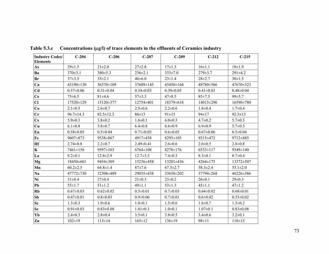
73
Table 5.3.c Concentrations (g/l) of trace elements in the effluents of Ceramics industry
Industry Codes/ Elements
C-204 C-206 C-207 C-209 C-212 C-215
As 29±1.5 21±2.0 27±2.8 17±1.3 16±1.1 18±1.9
Ba 370±3.1 380±5.3 236±2.1 333±7.0 279±3.7 291±4.2
Br 37±3.5 35±2.1 40±6.0 23±1.4 28±2.7 30±1.5
Ca 43190±130 36370±109 37689±145 45450±164 48780±566 47670±323
Cd 0.37±0.06 0.31±0.04 0.34±0.03 0.39±0.05 0.41±0.03 0.48±0.04
Ce 75±6.5 81±4.6 57±3.3 47±8.5 85±7.5 99±5.7
Cl 17520±129 15120±377 12754±401 18379±618 14015±296 16590±780
Co 2.1±0.5 2.6±0.7 2.5±0.6 2.2±0.6 1.8±0.4 1.7±0.4
Cr 96.7±14.3 82.5±12.3 86±13 91±15 94±17 92.3±13
Cs 5.9±0.3 3.8±0.2 1.6±0.1 6.0±0.3 4.7±0.2 5.7±0.3
Cu 6.1±0.8 5.8±0.7 6.4±0.8 6.6±0.9 6.9±0.9 5.7±0.5
Eu 0.58±0.05 0.5±0.04 0.71±0.03 0.6±0.05 0.67±0.06 0.5±0.04
Fe 9607±873 9538±867 4917±438 8293±103 9215±472 9712±885
Hf 2.74±0.8 2.2±0.7 2.49±0.41 2.6±0.6 2.0±0.5 2.8±0.8
K 7461±156 9597±103 6764±108 8278±176 6533±117 9349±140
La 9.2±0.1 12.8±2.9 12.7±3.3 7.4±0.3 8.3±0.1 8.7±0.4
Mg 18450±601 9454±389 15236±458 13201±436 4264±175 13372±507
Mn 60.2±2.5 64.8±1.4 87±7.6 67.5±2.7 58.3±2.4 55.1±2.0
Na 47772±730 32308±489 29035±438 33630±202 37794±268 46226±586
Ni 31±0.4 27±0.4 21±0.3 23±0.2 26±0.1 29±0.3
Pb 55±1.7 51±1.2 49±1.1 53±1.3 45±1.1 47±1.2
Rb 0.67±0.03 0.62±0.02 0.5±0.01 0.7±0.03 0.64±0.02 0.68±0.01
Sb 0.47±0.01 0.8±0.03 0.9±0.06 0.7±0.01 0.6±0.02 0.53±0.02
Sc 1.3±0.3 1.9±0.6 1.0±0.1 1.5±0.6 1.6±0.7 1.3±0.2
Se 0.91±0.03 0.83±0.08 1.01±0.3 1.0±0.1 1.07±0.1 0.83±0.08
Yb 2.4±0.3 2.8±0.4 3.5±0.1 3.8±0.5 3.4±0.6 3.2±0.1
Zn 102±19 113±14 165±12 136±19 98±11 110±15

74
Table 5.4.a Physical analysis of Textile/ Yarn industrial effluents, collected from industries of Faisalabad and Gujranwala
Industry Codes
Sample Volume
(ml)
Temp (C)
Wt. Of Dry Sample
(gm)
pH Density (gm/ml)
Electrical Conductivity EC
(ms/l)
Specific Gravity
TDS (ppm)
Turbidity (NTU)
T-501 540 57.3 01.479 10.10 1.00168 12.5 1.00072 5892 16.0 T-502 610 58.5 00.848 09.25 1.00104 32.0 1.00038 6194 19.5 T-503 570 59.1 09.571 10.50 1.01412 19.5 1.01315 7189 30.0 T-504 550 60.5 00.501 09.75 1.00188 10.0 1.00092 5144 44.5 T-505 590 56.2 01.799 11.00 1.00396 30.5 1.00299 7236 27.0 T-506 620 58.9 00.632 10.40 1.00316 23.0 1.00219 6726 17.0 T-507 630 60.4 01.201 09.10 1.00344 15.5 1.00248 4471 39.5 T-508 580 56.8 00.922 11.95 1.00252 24.0 1.00156 5038 20.0 T-509 560 59.4 00.086 10.80 1.00164 28.0 1.00068 4419 41.5 T-510 550 57.7 10.017 09.15 1.02432 33.5 1.02334 7645 16.5 T-511 565 58.6 02.857 10.25 1.00516 25.0 1.00421 6812 24.0 T-512 595 56.3 00.601 09.35 1.00141 11.5 1.00044 5863 37.5 T-513 615 60.3 03.291 11.90 1.00636 20.0 1.00539 6597 32.0 T-514 625 56.1 01.737 10.35 1.00284 35.0 1.00188 7563 29.0 T-515 585 59.2 13.619 09.20 1.03544 26.5 1.03445 5109 21.5 T-516 570 58.7 00.474 10.60 1.00174 17.5 1.00079 6912 38.5 T-517 555 56.5 00.412 09.30 1.00186 21.0 1.00091 5257 25.5 T-518 575 57.9 04.498 11.10 1.01116 13.0 1.01019 4558 28.0 T-519 580 59.9 02.021 10.15 1.00296 12.0 1.00199 6592 18.0 T-520 590 57.4 02.122 09.70 1.00392 21.5 1.00296 7828 41.0

75
Table 5.4.b Physical analysis of Pulp/ Paper industrial effluents, collected from industries of Faisalabad and Gujranwala
Industry Codes
Sample Volume
(ml)
Temp (C)
Wt. Of Dry Sample
(gm)
pH Density (gm/ml)
Electrical Conductivity
EC (ms/l)
Specific Gravity
TDS (ppm)
Turbidity (NTU)
P-311 520 41.0 3.000 06.3 1.0021 16 1.00279 4789 28 P-312 610 44.4 0.839 07.1 1.0033 26 1.00148 5338 37 P-313 550 42.6 0.819 08.3 1.0030 19 1.00112 7037 29 P-314 620 43.5 3.051 09.2 1.0042 31 1.00232 6445 51 P-315 530 45.0 0.811 06.5 1.0031 37 1.00128 7332 46 P-316 570 41.3 0.815 10.8 1.0027 28 1.00084 7419 33 P-317 540 42.7 0.934 07.4 1.0032 23 1.00132 5175 39 P-318 560 43.4 0.613 06.9 1.0036 33 1.00181 7256 44 P-319 630 41.8 0.717 09.7 1.0032 25 1.00136 7960 56 P-320 580 45.3 0.714 08.6 1.0036 29 1.00172 7567 53 P-321 610 44.2 1.496 06.7 1.0042 22 1.00423 9253 41 P-322 620 43.7 1.061 08.2 1.0033 40 1.00148 8695 48 P-323 560 44.6 0.954 10.3 1.0032 27 1.00132 8766 32 P-324 590 45.8 1.81 07.8 1.0033 34 1.00144 6253 36 P-325 580 41.9 0.752 06.4 1.0039 36 1.00204 6826 27 P-326 570 43.6 1.489 09.3 1.0035 18 1.00168 9626 25 P-327 540 42.2 1.424 08.4 1.0043 35 1.00248 6113 34 P-328 560 44.7 3.555 07.9 1.0040 38 1.00212 8697 31 P-329 590 42.5 8.497 07.5 1.0048 15 1.00295 6615 59 P-330 560 43.1 1.283 08.7 1.0031 32 1.00121 8589 38

76
Table 5.4.c Physical analysis of Ceramics industrial effluents, collected from industry of Gujranwala
Industry Codes
Sample Volume
(ml)
Wt of dry Samples
(gm)
Temp (C)
pH Density (gm/ml)
EC (ms/l)
TDS (ppm)
Specific Gravity
Turbidity (NTU)
C-201 560 1.105 26.0 8.20 1.01056 09.35 384 1.00722 08.55
C-202 600 1.755 27.5 9.00 1.01168 07.25 302 1.00833 21.50
C-203 540 1.157 28.2 8.10 1.01112 07.85 328 1.00777 29.55
C-204 630 0.826 26.4 8.50 1.00976 07.67 317 1.00642 08.30
C-205 500 2.145 30.0 9.90 1.01200 08.91 366 1.00865 31.55
C-206 560 1.000 29.8 9.30 1.01180 15.50 618 1.00845 11.90
C-207 520 5.215 28.7 8.80 1.01408 12.35 490 1.01072 53.65
C-208 565 0.804 29.5 8.00 1.01032 15.12 617 1.00698 11.25
C-209 615 2.686 26.3 9.50 1.01176 08.27 334 1.00842 34.70
C-210 520 1.396 27.2 8.60 1.01168 07.49 312 1.00833 17.50
C-211 610 0.860 28.4 8.90 1.01032 09.65 391 1.00701 16.05
C-212 620 1.840 29.6 9.40 1.01072 07.27 296 1.00738 31.00
C-213 510 0.932 26.6 9.80 1.01052 09.04 285 1.00718 10.15
C-214 620 1.246 27.7 9.20 1.01024 07.89 321 1.00691 12.25
C-215 550 1.008 29.3 8.40 1.00996 10.19 410 1.00662 16.65
C-216 555 0.826 28.1 8.70 1.00976 09.14 372 1.00642 12.90
C-217 545 0.931 29.9 9.80 1.01044 13.38 539 1.00711 14.20
C-218 560 0.900 28.6 8.30 1.01128 13.55 461 1.00794 13.25

77
5.4. Trace elemental contents in the Soils
All the soil samples, collected from Faisalabad and Gujranwala industrial areas,
were irrigated with industrial effluents. The selected fields for the present studies were
located in the vicinity of Peoples colony, Industrial estate, Nishatabad, Gulistan colony,
Sitara colony and Ghulam Muhammad-abad within the Faisalabad municipal corporation
limits. Moreover, the selected fields, for Gujranwala municipal corporation limits, were
Small industrial estate, Fatomand, Garjakh, Dhule, Satellite town and Muhammad Nagar.
200 soil samples were analyzed, through NAA and AAS techniques, for the present study.
Table 5.5 represents the results for the trace elements of soils (Top-soil St and Sub-soils
Ss), on which Faisalabad’s crops and vegetables (summer, winter and under-ground) were
grown. Similarly, the results for the trace elements of soils (Top soil St and Sub soils Ss),
on which Gujranwala’s crops, summer, winter and under-ground vegetables were
cultivated, are presented in Table 5.6. Concentrations (g/g) of trace elements in the
agriculture (non-industrial) soils of Islamabad and Rawalpindi zones are shown in Table
5.7. Those were used as blank references. Similarly, a comparison among the
concentrations (g/g) of trace elements in the international soils of India & Norway and
national soils of Faisalabad & Gujranwala are shown in Table 5.8.

78
Table 5.5 Concentrations (g/g) of trace elements in the soils of Faisalabad’s industrial areas
Places/ Elements
Peoples Colony-St
Peoples Colony –Ss
Industrial Estate-St
Industrial Estate –Ss
Sitara colony-St
Sitara colony –Ss
Ghulam Muhammad abad-St
Ghulam Muhammad abad-Ss
As 6.26±0.2 6.20±0.3 3.5±0.1 3.2±0.1 5.1±0.3 4.8±0.3 13.55±0.1 15.85±0.1 Ba 148±22 268±35 480±25 339±9.0 506±48 483±46 457±5.0 415±4.0 Br 5.57±0.7 4.36±0.5 3.27±0.29 5.9±0.6 2.9±0.1 4.4±0.3 3.42±0.39 1.77±0.23 Cd 0.31±0.01 0.37±0.03 0.39±0.02 0.51±0.05 0.41±0.03 0.46±0.05 1.32±0.2 0.38±0.03 Ce 76±12 62.8±2.2 98±16 52±8.3 72±16 62±15 61±1.0 83±1.0 Cl 647±17 619±16 1047±85 966±74 782±113 715±96 867±111 789±98 Co 11.6±0.2 10.6±0.2 10.78±0.3 7.2±0.2 12.4±0.8 14.8±1.2 7.8±0.1 8.1±0.1 Cr 66±4.5 85±6.1 66.7±2.15 60±1.5 79±24 73.6±22 138±1.0 133±1.0 Cs 8.4±0.5 7.4±0.4 6.8±0.9 4.7±1.0 7.5±0.3 8.5±0.4 5.02±0.2 4.98±0.2 Cu 27±4.7 25.1±5.3 37±3.4 31±3.1 32±2.8 26±2.1 41±2.7 34±1.9 Eu 1.3±0.02 0.99±0.01 1.05±0.17 0.7±0.05 1.32±0.04 1.06±0.02 0.85±0.06 1.1±00.1 Fe 30754±169 37142±292 27154±663 16935±303 33405±104 38174±127 21293±328 22196±349 Hf 7.7±0.5 8.8±0.6 4.37±0.1 4.95±1.0 6.0±0.1 7.2±0.2 5.07±0.3 4.91±0.3 K 16240±485 14460±389 26991±203 20250±234 30895±253 28916±167 20852±516 21577±538 La 119±3.5 56.3±1.2 30.6±2.68 23±2.1 68.7±2.0 43.8±1.6 29.4±0.4 48.3±0.8 Mg 2053±61 2294±39 7320±43 7445±75 3512±74 3718±71 4572±83 5893±95 Mn 470±76 383±30 756±79 503±5.4 543±12 581±13 544±5.2 498±4.7 Na 20208±472 31306±685 18310±342 19863±615 21690±950 22416±463 3941±258 11233±248 Ni 16±1.3 18±1.5 21±1.6 23±1.7 19±1.1 16±1.0 32±1.5 28±1.3 Pb 47±2.1 56±2.5 41±1.8 49±2.0 45±1.4 51±1.7 53±2.2 58±2.5 Rb 123±3.0 222±5.0 111±7.3 88±5.0 91±20 100±22 94±2.0 92±2.0 Sb 0.79±0.01 0.83±0.01 1.28±0.4 0.89±0.01 0.56±0.05 0.87±0.07 1.69±0.05 1.32±0.01 Sc 12.1±0.7 11.7±0.3 10.1±0.91 7.5±0.6 11.6±0.9 12.9±1.0 7.0±0.1 7.2±0.1 Se 3.2±0.5 3.1±0.6 1.97±0.1 1.51±0.1 1.22±0.6 1.67±0.9 3.28±0.7 3.31±0.7 Th 14±1.6 27±4.0 8.9±0.3 10.9±0.6 10.2±0.9 17.8±1.2 11.88±0.7 15.16±0.7 Ti 916±16 926±25 1707±95 1320±75 1018±66 1134±72 1542±78 1236±54 V 102±10 113±12 141±12.6 93.6±3.0 98±2.5 81±2.1 101±1.2 84±1.0 Yb 3.3±0.1 4.1±0.5 3.2±0.1 1.6±0.1 3.2±0.1 4.1±0.1 2.07±0.1 2.33±0.2 Zn 89±5.8 58±3.2 206±24 131±3.8 107±32 226±57 82±11 67±13 Zr 248±16 257±17 227±19 171±32 493±27 530±29 380±6.0 172±4.0

79
Table 5.6 Concentrations (g/g) of trace elements in the soils of Gujranwala’s industrial areas
Places/ Elements
Small Industrial Estate-St
Small Industrial Estate –Ss
Dhula-St Dhula –Ss Muhammad Nagar-St
Muhammad Nagar –Ss
Garjakh-St Garjakh-Ss
As 4.58±0.4 4.27±0.3 8.1±0.8 8.9±0.8 6.3±0.5 6.9±0.6 18.7±0.72 14.3±0.19
Ba 235±32 238±33 549±48 589±68 277±46 284±43 216±3.7 242±4.2 Br 3.13±0.6 3.95±0.4 4.7±0.5 5.1±0.4 3.2±0.2 3.9±0.3 6.9±0.3 10.8±1.3 Cd 0.56±0.08 0.63±0.08 0.49±0.04 0.54±0.05 0.59±0. 0.71±0.06 1.68±0.04 0.77±0.06 Ce 95±16 107±17 80±19 61±14 54±12 43±10 52.1±1.8 139±12.6 Cl 586±68 207±53 824±36 485±21 631±26 349±14 512±17 478±14 Co 9.7±0.8 12.6±0.3 14.9±1.9 13.9±1.1 9.1±0.6 10.7±0.7 16.5±0.4 17.7±0.4
Cr 106±6.9 144±10 145±42 195±57 213±63 293±86 86±0.8 76±0.6 Cs 6.3±0.2 8.1±0.2 6.4±2.2 6.5±1.9 5.9±0.3 6.2±0.3 5.24±0.5 5.9±0.5 Cu 14.2±1.9 23.1±2.6 12.1±1.2 21.3±3.0 17.2±1.6 26.3±1.4 19.5±1.2 28.1±1.6 Eu 0.88±0.02 1.0±0.1 1.45±0.3 1.24±0.3 0.9±0.02 0.8±0.02 0.92±0.07 0.86±0.06 Fe 31910±290 39065±424 35318±117 34768±112 25422±763 27805±931 19855±118 12250±109 Hf 9.8±0.8 8.6±0.5 4.8±0.3 5.5±0.4 4.1±0.2 5.7±0.2 8.4±0.1 7.9±0.5
K 17768±199 16540±133 26760±200 23180±190 19560±161 21805±179 33483±276 44800±369 La 46.8±1.2 43.94±1.8 56.1±1.2 52±1.1 48±0.8 42±0.6 41±2.0 82±5.0 Mn 507±25 384±21 470±11 433±10 419±9.0 315±7.0 320±4.9 368±10
Na 8422±102 8404±122 10805±475 11180±490 10785±425 10675±465 2168±20.4 2703±25.4
Ni 51±4.7 59±4.9 36±1.3 42±1.4 44±1.5 49±1.5 33±1.1 39±1.3
Pb 72±5.5 78±5.7 64±2.3 67±2.7 61±1.8 69±2.0 74±3.2 79±3.8
Rb 171±6.0 205±4.0 144±12.1 146±12.2 120±10.1 113±9.5 112±19.6 169±29.7
Sb 1.3±0.2 1.6±0.3 0.65±0.05 0.57±0.05 1.21±0.1 1.38±0.1 1.11±0.1 1.23±0.1
Sc 10.4±0.2 12.6±0.5 10.5±0.7 9.5±0.8 7.4±0.5 8.4±0.6 8.1±0.5 9.3±0.6 Se 3.5±0.8 2.9±0.3 1.68±0.1 0.32±0.02 1.16±0.6 1.03±0.5 1.76±0.05 1.6±0.05 Yb 3.9±0.2 4.3±0.1 3.7±0.7 3.0±0.6 2.3±0.05 3.9±0.7 3.34±0.08 3.21±0.04 Zn 355±3.0 452±5.0 111±13 170±5.0 361±11 357±17 50.6±0.9 44±7.0 Zr 250±13.5 246±17 339±34 212±30 342±76 362±20 268±6.3 235±42

80
Table 5.7 Concentrations (g/g) of trace elements in the agriculture soils of Islamabad and Rawalpindi Non-industrial zones
Places/ Elements
Rawalpindi –St Rawalpindi –Ss Islamabad-St Islamabad-Ss
Al 35592±345 34468±298 35968±317 33998±277 As 14.1±1.6 12.8±1.1 14.4±1.8 12.9±1.2 Ba 762±39 659±32 826±43 734±35 Br 8.6±0.81 9.3±0.92 9.1±0.91 9.9±0.95 Ca 3183±226 3527±237 3691±243 3978±258 Ce 78±8.0 70±7.0 66±6.0 59±5.0 Cl 616±25 692±27 732±30 763±33 Co 9.3±0.9 8.1±0.8 7.9±0.7 7.2±0.6 Cr 56±9.0 75±12 81±10 96±14 Cs 8.9±0.8 10.2±0.9 8.2±0.7 9.9±0.8 Cu 46±4.6 33±2.8 52±5.1 41±3.9 Eu 0.98±0.03 0.76±0.02 1.3±0.1 1.0±0.1 Fe 29763±389 40536±417 27456±367 38967±395 Hf 3.9±0.8 0.77±0.04 2.6±0.7 0.83±0.05 K 15678±235 19325±257 16519±239 20168±263 La 23.7±9.2 31.7±9.4 32.2±9.5 38.6±9.7 Mg 31578±467 33296±478 35367±483 38593±488 Mn 772±55 528±36 666±42 505±31 Na 8362±144 8897±167 7816±152 8274±161 Nd 35.3±4.3 31.6±3.7 48.3±4.9 43.2±4.5 Rb 58±6.1 74±7.2 65±6.3 81±7.8 Sb 2.1±0.1 0.18±0.06 2.4±0.1 2.2±0.1 Sc 10.2±1.3 8.7±0.8 12±1.1 11.3±1.0 Se 0.84±0.06 0.63±0.03 1.3±0.2 0.96±0.07 Ta 1.0±0.1 0.36±0.04 1.26±0.1 0.74±0.05 Th 2.4±0.21 2.1±0.2 3.1±0.3 2.7±0.24 Ti 1126±39 1065±31 1374±43 1115±37 V 81.6±9.4 71.9±8.1 97.2±9.9 88.3±9.2 Yb 2.9±0.2 1.64±0.1 2.8±0.21 1.5±0.1 Zn 96.7±3.1 79.4±2.5 121±4.7 100±4.2 Zr 117±5.2 73±3.0 84±3.4 69±2.8

81
Table 5.8 A comparison among the concentrations (g/g) of trace elements in the international and national soils
Places/ Elements Faisalabad Gujranwala India Norway
As 13.55 18.7 18.17 14.6 Ba 457 216 838 2261 Br 3.42 6.9 1.85 3.71 Cl 867 512 732 795 Co 7.8 16.5 23.86 22 Cr 138 86 85.83 63 Cs 5.02 5.24 13.85 4.6 Fe 21293 19855 38800 36940 Hf 5.07 8.4 2.85 14.1 K 20852 33483 23000 14550 La 29.4 41 32.55 108 Mg 4572 36654 1666 41050 Mn 544 320 1360 5054 Na 3941 2168 4200 2765 Rb 94 112 100.74 68.5 Sb 1.69 1.11 2.4 2.6 Sc 7.0 8.1 12.13 10.79 Se 3.28 1.76 1.3 2.0 Th 11.88 4.6 13.88 6.5 Yb 2.07 3.34 2.24 1.8 Zn 82 50.6 66 146 Zr 380 268 230 360

82
5.5. Trace elemental contents in the crops
Crops (wheat, rice, maize and millet) were collected from industrial areas of
Faisalabad & Gujranwala and analyzed for the trace elemental concentrations. Twenty-
two elements were determined in each sample of human edible portion, which included
essential, non-essential, rare earth and toxic elements. Elemental concentrations are given
in Tables 5.9.a & b for crops (edible portions) collected from Faisalabad and Gujranwala
respectively. Similarly twenty-eight elements were determined which included essential
non-essential, rare earth and toxic elements in Faisalabad or Gujranwala’s crops leaves
(edible portion for animals). Tables 5.10.a & b show the concentrations (g/g) of trace
elements in the crops leaves collected from Faisalabad and Gujranwala respectively.
Table 5.9.a Concentrations (g/g) of trace elements in Faisalabad’s crops (Fruits)
Crops/Elements Wheat Rice Maize Millet As 0.16±0.4 0.18±0.02 0.43±0.01 0.79±0.03 Ba 6.9±0.4 5.0±0.2 1.6±0.1 2.1±0.1 Br 2.1±0.1 0.9±0.1 4.12±0.2 1.2±0.05 Cd 0.1±0.01 0.05±0.01 1.5±0.6 1.2±0.5 Ce 0.38±0.02 0.4±0.01 1.11±0.1 0.16±0.01 Cl 846±31 399±28 393±22 469±36 Co 0.018±0.003 0.1±0.01 0.03±0.001 0.06±0.004 Cr 0.7±0.04 1.7±0.3 2.5±0.3 9.63±1.3 Cs 0.04±0.001 0.01±0.005 0.05±0.001 0.07±0.01 Cu 14.2±1.2 8.1±1.0 3.9±0.4 17.8±2.3 Eu 0.02±0.001 0.01±0.003 0.03±0.001 0.32±0.07 Fe 217±26 120±1.0 136±1.5 163±7.0 Hf 0.25±0.02 0.01±0.001 0.03±0.001 0.01±0.001 K 1292±102 2229±132 4124±128 5588±544 La 0.86±0.02 0.11±0.06 0.72±0.03 0.21±0.01 Mn 33.7±2.6 9.9±0.2 7.4±0.3 46.5±1.0 Na 669±41 337±47 15.9±1.8 52.9±3.9 Ni 0.24±0.04 4.3±0.6 5.1±0.9 3.6±0.8 Pb 0.48±0.07 2.36±0.3 4.3±0.2 2.7±0.1 Rb 2.1±0.2 0.6±0.02 1.12±0.3 0.25±0.04 Sb 0.03±0.001 0.05±0.004 0.02±0.001 0.04±0.002 Sc 0.05±0.001 0.01±0.001 0.3±0.01 0.05±0.003 Se 0.28±0.06 0.6±0.06 0.2±0.01 1.03±0.01 Yb 1.4±0.05 0.8±0.01 0.5±0.02 0.3±0.01 Zn 27±2.0 48±4.1 28±1.0 18.5±2.9

83
Table 5.9.b Concentrations (g/g) of trace elements in Gujranwala’s crops (Fruit)
Crops/ Elements
Wheat Rice Maize Millet
As 0.32±0.02 0.31±0.02 0.47±0.03 0.4±0.01
Ba 4.6±0.1 7.2±0.3 2.1±0.1 3.6±0.2
Br 3.42±0.34 1.4±0.1 2.38±0.6 6.2±0.1
Cd 0.08±0.006 0.09±0.004 1.3±0.3 0.6±0.01
Ce 0.53±0.07 0.31±0.02 2.0±0.1 0.23±0.01
Cl 277±44 357±13 416±26.8 831±85
Co 0.04±0.003 0.11±0.01 0.05±0.001 0.06±0.001
Cr 0.39±0.01 0.65±0.08 4.9±0.68 5.3±0.1
Cs 0.09±0.005 0.026±0.002 0.07±0.009 0.03±0.001
Cu 15.5±1.6 9.9±1.1 6.0±0.5 18.3±1.4
Eu 0.1±0.01 0.06±0.001 0.073±0.008 0.17±0.01
Fe 540±11 233.7±1.5 177.7±4.5 169±7.2
Hf 0.07±0.001 0.29±0.01 0.24±0.05 0.1±0.01
K 1966±159 1642±30 4687±86 5966±101
La 0.6±0.02 0.1±0.01 0.9±0.04 0.36±0.05
Mn 40±3.0 8.65±0.3 9.6±0.2 44.2±2.7
Na 345±27 123±11.6 10.4±0.1 39.7±1.2
Ni 0.36±0.06 4.9±0.8 4.8±0.9 1.7±0.3
Pb 0.61±0.09 3.84±0.27 4.9±0.8 2.3±0.4
Rb 2.7±0.6 6.8±0.9 7.13±0.12 0.8±0.02
Sb 0.08±0.005 0.03±0.002 0.053±0.003 0.04±0.001
Sc 0.04±0.001 0.04±0.003 0.31±0.07 0.05±0.002
Se 0.6±0.01 1.1±0.2 1.1±0.1 1.07±0.3
Ta 0.3±0.01 0.48±0.01 0.21±0.02 0.5±0.02
Tb 0.2±0.01 0.4±0.01 0.031±0.001 0.01±0.001
Th 0.08±0.002 0.57±0.01 0.42±0.01 0.63±0.01
Yb 1.2±0.01 0.69±0.05 0.17±0.03 0.11±0.01
Zn 45.2±4.5 22.3±3.9 32.1±4.15 39±1.0
Zr 15.6±2.0 29±1.8 7.66±0.16 10.6±0.1

84
Table 5.10.a Concentrations (g/g) of trace elements in Faisalabad’s crops (Leaves)
Crops/
Elements
Wheat Rice Maize Millet
As 1.3±0.05 2.74±0.2 0.82±0.02 0.58±0.06
Ba 36.4±0.3 27.8±0.4 6.4±0.4 19.4±0.9
Br 23.7±3.8 5.8±0.2 4.76±0.2 23.5±0.5
Ce 1.96±0.38 1.23±0.1 1.91±0.2 0.33±0.04
Cl 6223±270 5723±43 818±31 4984±392
Co 0.41±0.01 0.81±0.05 0.06±0.001 0.18±0.01
Cr 8.97±1.0 3.1±0.2 4.1±0.4 16.1±0.22
Cs 0.32±0.03 0.12±0.03 0.07±0.01 0.03±0.001
Eu 0.18±0.01 0.2±0.01 0.06±0.003 0.12±0.02
Fe 917±10 713±29 271±21 251±10
Hf 0.08±0.006 0.6±0.04 0.21±0.01 0.1±0.01
K 1966±68 1583±38 5536±31 7522±27
La 5.37±0.5 1.0±0.1 7.2±0.8 0.31±0.08
Mn 26.9±1.7 18.4±0.4 13.6±1.0 60±4.9
Na 319±8.0 1451±22 88±4.3 577±27
Rb 4.5±0.6 5.83±0.1 2.98±0.6 0.8±0.01
Sb 0.37±0.05 0.36±0.04 0.04±0.002 0.09±0.01
Sc 0.025±0.001 0.15±0.01 0.7±0.03 0.08±0.001
Se 0.2±0.04 0.23±0.07 0.32±0.02 0.1±0.02
Ta 0.03±0.002 0.7±0.04 0.09±0.01 0.07±0.001
Tb 0.02±0.001 0.07±0.002 0.04±0.001 0.06±0.01
Th 0.33±0.01 0.21±0.05 0.06±0.003 0.13±0.01
Yb 0.06±0.004 0.12±0.03 0.08±0.004 0.56±0.01
Zn 39.9±6.4 50.7±1.9 36±2.1 27.5±1.0
Zr 2.86±0.4 4.5±0.3 9.3±0.8 0.7±0.01

85
Table 5.10.b Concentrations (g/g) of trace elements in Gujranwala’s crops
(Leaves)
Crops/ Elements
Wheat Rice Maize Millet
As 1.8±0.1 1.6±0.13 2.1±0.4 0.6±0.01
Ba 14.7±0.3 36.2±0.6 23.1±1.3 11.8±1.0
Br 4.5±0.36 19.9±0.8 1.52±0.08 17.0±0.8
Ce 0.52±0.07 3.1±0.2 4.36±0.48 0.36±0.03
Cl 253±49 4047±30 711±15 6352±98
Co 0.52±0.05 0.88±0.05 0.08±0.001 0.6±0.01
Cr 2.88±0.2 2.0±0.1 10.19±1.3 24.8±0.3
Cs 0.11±0.02 0.38±0.03 0.103±0.07 0.05±0.01
Eu 0.18±0.02 0.3±0.02 0.086±0.007 0.1±0.02
Fe 488±18 154±6.9 165±6.2 225±39
Hf 0.046±0.002 0.15±0.01 0.24±0.09 0.1±0.01
K 38321±568 2269±49 5219±57 6284±98
La 0.51±0.06 0.6±0.02 0.8±0.02 0.4±0.01
Mn 27±2.0 61.7±8.8 23.86±4.25 47.4±2.9
Na 723±29 1167±15.7 95±2.5 47±3.4
Rb 9.6±0.2 14.6±0.57 16.14±0.69 0.14±0.03
Sb 0.03±0.001 0.13±0.01 0.064±0.004 0.06±0.001
Sc 0.012±0.001 0.47±0.03 0.54±0.07 0.1±0.01
Se 0.18±0.01 0.53±0.01 0.16±0.08 0.15±0.01
Ta 0.15±0.02 0.07±0.001 0.03±0.003 0.3±0.02
Tb 0.02±0.001 0.058±0.003 0.082±0.002 0.04±0.001
Th 0.13±0.03 0.61±0.01 0.04±0.002 0.07±0.001
Yb 0.37±0.01 0.11±0.001 0.08±0.004 0.4±0.01
Zn 69±6.0 38.7±0.7 43±3.9 17±1.0
Zr 48.9±1.1 17.4±0.6 13.63±0.29 1.6±0.1

86
5.6. Trace elemental contents in the vegetables
Twelve different types of vegetables were collected during various seasons within
the vicinity of industrial areas of Faisalabad and Gujranwala. Concentrations (µg/g) of
trace elements in edible portions of summer vegetables (brinjal, tomato, bitter gourd,
ridye gourd & pumpkin), winter vegetables (mustard, cabbage, & spinach) and under
ground vegetables (potato, turnip, radish and carrot) were determined. In each sample,
more than thirty trace elements were analyzed, qualitatively and quantitatively. These
include major nutrients, essential, non-essential, toxic and rare earth elements. The
concentrations (g/g) of trace elements in edible portions for Faisalabad and
Gujranwala’s summer/ winter vegetables are presented in Tables 5.11.a & b and 5.12.a &
b respectively.
Table 5.11.a Concentrations (g/g) of trace elements in Faisalabad’s summer vegetables (Edible portion)
Names/ Elements
Brinjal Tomato Bitter gourd Ridye gourd Pumpkin Mustard
As 0.49±0.01 0.53±0.04 0.35±0.01 0.72±0.06 0.64±0.02 2.5±0.9
Ba 9.6±0.1 5.43±0.18 72±4.0 15±3.0 26±2.1 39±2.8
Br 24.8±1.6 65±3.8 6.3±0.5 18.6±0.2 11.1±0.2 47±1.5
Cd 0.08±0.001 0.08±0.002 0.05±0.001 0.07±0.001 0.1±0.01 0.12±0.01
Ce 0.76±0.1 0.16±0.01 0.5±0.01 0.5±0.01 0.8±0.02 1.2±0.1
Cl 982±31 1279±74 1812±39 1698±68 1624±23 1967±43
Co 0.29±0.02 0.4±0.02 0.17±0.01 0.13±0.02 0.2±0.01 0.68±0.07
Cr 1.37±0.5 1.67±0.02 4.4±0.2 7.1±0.1 8.3±0.6 5.2±0.6
Cs 0.1±0.03 0.3±0.01 0.19±0.01 0.08±0.001 0.01±0.001 0.04±0.003
Cu 6.5±0.3 11.3±0.01 10.2±0.1 5.2±0.2 9.1±0.7 7.4±0.5
Eu 0.021±0.001 0.02±0.001 0.09±0.003 0.06±0.001 0.04±0.01 0.01±0.004
Fe 587±21 250±21 372±10 598±37 267±26 1117±18
Hf 0.21±0.05 0.12±0.01 0.04±0.003 0.32±0.06 0.03±0.001 0.08±0.001
K 2871±303 5761±515 3325±457 1265±135 3328±288 2087±261
La 0.3±0.01 1.48±0.26 0.6±0.06 0.43±0.02 0.1±0.01 0.3±0.05
Mn 11±1.2 13±1.3 38±2.6 34±1.8 15±0.8 42±6.0

87
Na 1154±137 1624±186 3987±154 284±33 172±17 383±47
Ni 1.6±0.1 1.5±0.1 2.3±0.1 1.9±0.1 2.7±0.2 1.5±0.1
Pb 0.8±0.01 0.3±0.01 1.1±0.1 0.5±0.02 0.9±0.02 0.1±0.01
Rb 6.1±0.2 33.4±1.0 10.2±0.1 11±0.1 20±1.0 10.9±1.2
Sb 0.03±0.001 0.03±0.001 0.06±0.004 0.06±0.006 0.08±0.001 0.1±0.01
Sc 0.16±0.08 0.04±0.004 0.08±0.006 0.04±0.002 0.03±0.001 0.1±0.01
Se 0.24±0.01 0.11±0.05 0.08±0.001 0.11±0.01 0.18±0.01 0.21±0.02
Ta 0.3±0.01 0.5±0.01 1.1±0.1 0.01±0.001 0.03±0.001 0.04±0.001
Th 0.11±0.01 0.14±0.01 0.03±0.001 0.03±0.002 0.02±0.001 0.05±0.002
Yb 0.12±0.01 0.6±0.01 1.3±0.1 0.08±0.003 0.05±0.001 0.1±0.02
Zn 34±3.0 47.8±2.6 111±2.0 65±8.0 34±2.0 207±19
Table 5.11.b Concentrations (g/g) of trace elements in Faisalabad’s winter & underground vegetables (Edible portion)
Names/ Elements
Cabbage Spinach Potato Turnip Radish Carrot
As 2.73±0.34 0.52±0.02 0.36±0.02 0.22±0.02 0.43±0.05 0.73±0.01 Ba 23.7±1.6 10.5±1.1 8.9±0.3 27±4.0 23±4.0 13±1.0 Br 4.3±0.2 32±1.6 11.4±0.9 26±5.0 19.9±1.3 35.8±3.1 Cd 1.1±0.01 0.1±0.01 0.2±0.01 0.09±0.001 0.4±0.01 0.4±0.01 Ce 0.78±0.3 0.4±0.01 3.7±0.5 0.8±0.05 0.3±0.01 0.1±0.01 Cl 1438±136 6321±237 783±9.0 872±18 1287±15 3267±44 Co 0.25±0.01 0.11±0.03 0.1±0.01 0.3±0.04 0.07±0.003 0.65±0.02 Cr 1.4±0.52 2.8±0.1 1.3±0.3 1.9±0.2 2.4±0.3 0.8±0.05 Cs 0.02±0.006 0.1±0.03 0.9±0.1 0.2±0.01 0.22±0.03 0.14±0.01 Cu 8.1±0.7 21±1.2 4.8±0.2 4.7±0.2 4.1±0.2 2.1±0.1 Eu 0.01±0.001 0.4±0.02 0.01±0.003 0.01±0.002 0.01±0.001 0.05±0.001 Fe 172±11 389±26 63±7.0 121±6.0 110±4.0 123±6.0 Hf 0.02±0.003 0.06±0.001 0.21±0.02 0.32±0.04 0.24±0.03 0.22±0.02 K 1718±177 3725±328 2593±362 2835±326 4649±245 3129±561 La 3.79±0.1 0.1±0.01 3.6±0.3 0.05±0.004 0.06±0.001 0.4±0.01 Mn 13.7±1.4 22±2.3 10.5±0.8 6.9±0.4 9.7±1.0 8.3±0.1 Na 2732±343 4893±316 2166±113 2366±141 1669±129 2236±151 Ni 1.1±0.1 2.6±0.1 1.8±0.1 1.0±0.1 0.7±0.01 2.1±0.1 Pb 2.3±0.2 2.1±0.1 3.4±0.2 0.07±0.001 0.08±0.001 0.5±0.02 Rb 2.85±0.84 15.5±1.6 13±1.0 29±3.0 10.6±0.5 4.4±0.2 Sb 0.01±0.001 0.02±0.005 0.06±0.002 0.05±0.002 0.04±0.001 0.09±0.001 Sc 0.01±0.001 0.03±0.001 0.01±0.001 0.04±0.001 0.02±0.001 0.06±0.001 Se 0.09±0.008 0.06±0.002 0.1±0.02 0.05±0.002 0.03±0.001 0.02±0.001 Ta 0.28±0.04 0.7±0.02 3.4±0.2 1.6±0.1 1.0±0.1 0.3±0.01 Th 0.23±0.01 0.26±0.01 0.04±0.001 0.38±0.05 0.06±0.001 0.02±0.001 Yb 0.07±0.003 0.4±0.01 0.7±0.01 1.1±0.1 1.9±0.1 0.8±0.02 Zn 59±3.6 42±1.8 51±3.0 42±2.0 37±3.0 20±1.0 Zr 4.8±0.3 7.1±0.21 0.4±0.01 0.57±0.04 0.26±0.05 0.08±0.001

88
Table 5.12.a Concentrations (g/g) of trace elements in Gujranwala’s summer vegetables (Edible portion)
Names/ Elements
Bitter gourd Tomato Brinjal Ridye gourd
Pumpkin Mustard
As 0.2±0.02 0.44±0.03 0.26±0.01 0.64±0.02 0.8±0.01 2.1±0.8
Ba 53±3.0 5.7±0.45 11.3±0.2 16±2.0 21±1.0 33.2±3.4
Br 9.4±0.1 52±2.9 19.6±1.3 14.9±0.1 16.4±0.4 35±1.4
Cd 0.07±0.001 0.1±0.01 0.09±0.001 0.11±0.01 0.09±0.001 0.18±0.01
Ce 0.26±0.01 0.22±0.01 0.88±0.01 0.4±0.05 0.72±0.01 1.75±0.16
Cl 725±44 698±61 547±56 1832±63 1377±42 1252±26
Co 0.21±0.04 0.5±0.01 0.35±0.02 0.27±0.05 0.15±0.03 0.49±0.01
Cr 5.7±0.8 2.68±0.02 11.6±0.05 6.2±0.5 9.7±0.7 3.7±0.3
Cs 0.13±0.02 0.5±0.06 0.12±0.01 0.06±0.001 0.01±0.002 0.09±0.004
Cu 11.5±1.0 12.2±0.6 8.3±0.5 6.7±0.3 11.3±0.9 8.9±0.4
Eu 0.08±0.001 0.03±0.002 0.03±0.002 0.04±0.002 0.07±0.002 0.05±0.001
Fe 222±30 347±33 651±27 766±24 210±38 1021±225
Hf 0.03±0.001 0.1±0.01 0.41±0.07 0.13±0.01 0.02±0.001 0.1±0.01
K 3265±318 5622±364 2456±254 2071±136 3143±193 3161±185
La 0.8±0.07 1.3±0.2 0.1±0.01 0.5±0.03 0.7±0.02 1.3±0.1
Mn 45.3±2.0 10±1.0 9.0±0.03 28.3±1.4 11.25±2.0 68±3.8
Na 3379±326 1596±118 1036±83 215±20 204±15 408±67
Ni 3.1±0.1 1.9±0.1 2.1±0.1 2.3±0.2 3.1±0.3 1.9±0.1
Pb 1.7±0.1 0.5±0.01 0.9±0.01 0.9±0.04 1.1±0.1 0.2±0.01
Rb 9.4±0.3 40±1.3 5.1±0.1 9.0±0.6 12.7±3.0 13.3±0.4
Sb 0.1±0.01 0.08±0.001 0.05±0.004 0.03±0.005 0.13±0.02 0.07±0.001
Sc 0.06±0.001 0.09±0.01 0.2±0.06 0.04±0.007 0.024±0.003 0.24±0.01
Se 0.1±0.01 0.18±0.02 0.29±0.08 0.25±0.02 0.14±0.05 0.32±0.01
Ta 2.02±0.01 0.7±0.01 0.14±0.01 0.02±0.005 0.06±0.001 0.07±0.001
Th 0.02±0.002 0.23±0.02 0.15±0.03 0.04±0.001 0.047±0.002 0.33±0.01
Yb 1.05±0.1 0.9±0.01 0.16±0.04 0.07±0.001 0.048±0.01 0.09±0.01
Zn 99.8±7.0 80±2.0 35±4.0 55±1.0 43±3.0 143±25
Zr 19.5±1.0 10.8±2.1 15±1.3 14.2±1.0 22.2±2.0 8.68±0.2

89
Table 5.12.b Concentrations (g/g) of trace elements in Gujranwala’s winter &
underground vegetables (Edible portion)
Names/ Elements
Cabbage Spinach Potato Turnip Radish Carrot
As 1.9±0.1 0.94±0.06 0.3±0.01 0.4±0.02 0.26±0.02 0.68±0.05
Ba 19.7±0.48 15.2±0.1 7.9±0.2 5.2±0.4 11±1.0 8.0±0.1
Br 10.6±0.8 26±1.9 7.9±1.0 47±8.0 15.2±2.0 27.8±2.4
Cd 1.4±0.1 0.3±0.02 0.3±0.01 0.12±0.01 0.5±0.01 0.51±0.02
Ce 0.59±0.03 1.0±0.1 2.5±0.4 0.5±0.01 0.09±0.006 0.07±0.001
Cl 1267±116 5248±253 1186±82 1132±24 1694±23 28312±161
Co 0.19±0.01 0.46±0.03 0.08±0.002 0.18±0.01 0.04±0.004 0.4±0.03
Cr 1.05±0.05 3.8±0.1 0.96±0.01 1.4±0.1 1.5±0.1 0.47±0.04
Cs 0.02±0.001 0.3±0.01 0.68±0.02 0.6±0.02 0.08±0.001 0.05±0.001
Cu 9.1±0.8 27±2.1 7.1±0.3 5.8±0.3 5.3±0.4 2.5±0.1
Eu 0.02±0.001 0.7±0.01 0.007±0.0001 0.008±0.0006 0.009±0.0003 0.03±0.001
Fe 279±13 441±72 82±5.0 94±8.0 120±7.0 136±4.0
Hf 0.01±0.001 0.09±0.001 0.11±0.01 0.17±0.01 0.25±0.02 0.21±0.03
K 1136±124 4832±261 23364±121 37569±428 33982±211 25664±123
La 2.1±0.1 0.3±0.02 2.3±0.2 0.07±0.001 0.04±0.001 0.3±0.01
Mn 10±0.1 16±0.3 9.3±0.5 8.4±0.7 4.6±0.1 5.7±0.1
Na 2165±145 4126±156 1649±107 6697±328 3698±334 9472±324
Ni 1.8±0.1 3.2±0.1 2.1±0.1 1.3±0.1 0.9±0.01 3.2±0.2
Pb 2.8±0.3 3.3±0.1 5.2±0.4 0.09±0.001 0.12±0.01 0.6±0.03
Rb 3.1±0.2 18.5±0.4 9.6±0.6 25±1.0 8.8±0.3 5.1±0.1
Sb 0.02±0.001 0.04±0.001 0.04±0.001 0.02±0.001 0.03±0.001 0.6±0.03
Sc 0.03±0.002 0.05±0.003 0.008±0.0007 0.01±0.001 0.02±0.002 0.05±0.002
Se 0.06±0.002 0.08±0.005 0.06±0.005 0.02±0.001 0.04±0.001 0.03±0.002
Ta 0.3±0.03 0.5±0.08 3.0±0.2 1.3±0.1 0.8±0.06 0.17±0.01
Th 0.33±0.02 0.37±0.03 0.1±0.01 0.24±0.02 0.06±0.003 0.02±0.001
Yb 0.17±0.08 0.5±0.08 0.5±0.02 1.6±0.1 1.3±0.1 0.5±0.05
Zn 86±1.8 56±3.0 46±4.0 40±1.0 57±1.5 19±1.0
Zr 4.6±0.4 8.9±0.2 0.1±0.01 0.25±0.05 0.15±0.04 0.08±0.005
90
CHAPTER-6
6. TREATMENT OF INDUSTRIAL EFFLUENTS
6.1. Introduction
Environmental protection is a critical part for the operation of chemical plants in
industrialized countries. So it is significant to focus on the environmental regulations in
major industrialized cities, their influence and implementation on the treatment of residues
and effluents. The industrial effluents violated the standard quantities of diverse
ingredients. Unprocessed discharge of the effluents is a cognizable offence under the
Environmental Protection Act 1997. The industries were releasing their effluents in the
streams, which pass through various villages posing severe health risk to the people,
animals and plants. Due to improved agriculture production, a number of agricultural based
industries have been established which are producing solid wastes and wastewater as a
byproduct in large quantity. These are liable for pollution/ contamination of the
surrounding soils, ground water and environment. Appropriate treatment and release of
industrial effluent is a growing concern as environmental awareness increases. The
prerequisite of a treatment plant is to protect the ecology of the surrounding areas from
adverse effects of industrial effluents. The pollution management and adoption of clean
technologies in the industries are to be the strategies to trim down the accessible pollution
load and will also have to sustainable industrial development in Pakistan.
6.2 Objectives of effluent treatment
The significant objectives for the management of industrial effluents are
summarized as below:

91
1. Smooth flow of effluents
2. Decontamination of oil and grease
3. Separation of suspended solids
4. Removal of heavy metals
5. Elimination or reduction of organic materials
6. Reduction of toxic compounds
7. Minimization of pollution load
8. Protection of soil and environment from pollution
9. Supply of treated industrial wastewater (without contaminations) for irrigation
6.3. Utilization of fresh water in the industries
Water is essential in industry for the following disciplines:
1. Industrial Processes
2. Product washing
3. Cleaning of raw materials
4. Plant and equipment washing
5. Steam generation
6. Cooling systems
7. Personnel consumption and sanitation
8. Air conditioning
6.4. Industrial wastewater pollution
Industrial effluents (wastewater) pollution is one of the major significant
environmental issues [132-133]. The term pollution is derived from the Latin word
“Pollutus”. “Pol” means before and “lutus” means wash. Industrial effluents contain
dissolved solids, suspended solids, organic/ inorganic compounds, oils, fat etc. Most of the
pollution creating industries is sugar, textile, pulp & paper, chemicals, fertilizers, tanneries
etc. The effluents of these industries are including large quantities of organic matter.
Organic pollution levels of effluents are measured in terms of Bio-chemical Oxygen
92
Demand (BOD) and Chemical Oxygen Demand (COD) values. The industries situated in
Faisalabad and Gujranwala regions release high levels of heavy metals, solids, organic
materials, dyes and salts directly into the municipal sewerage system for dumping into the
River Chanab and agricultural lands. Effluents of textile and yarn industries include acids,
caustic soda, organic materials (starch, wax, urea and ammonia), dyes, pigments,
detergents, cotton fiber and cuttings, bleaching agents, sodium hydroxide etc. Effluent of
paper and pulp industry contains chlorine, sulfides, cellulose, sulfite, sodium hydroxide,
resins, cotton waste, lignin, sludge etc. The effluent of ceramics industry enclosed alumina,
lime, magnesia, alkali, titania, silica, oxides of iron, chromium, manganese etc.
6.5. Need for the pollution control in the industry [134-138]
Textile and paper processing/ printing plants utilize a wide range of dyes and other
chemicals such as acids, bases, salts, detergents, wetting agents, stripping agents etc. Many
of these are not preserved in the final product and are released with the effluent. Usually
textile processing water usage is 150-1400 liters per kilogram of the product. The discharge
of industrial effluents to the environment may have severe and long-lasting consequences.
The effects and specific types of pollution in industrial effluents may generate problems.
6.6. Technologies for the treatment of industrial effluents
Treatment of industrial effluents is essential to protect human health and
environmental worth. To this consequence, the chosen technology should be cost effective,
simple and easy to operate and maintain. The remediation technologies embrace biological,
mechanical, electro-chemical, chemical and thermal means to detoxify the pollutants. Such
main classes of technical approaches differ significantly in their applicability to arrest the
problems because of both site and specific conditions. Bio-remediation appears to be the

93
secure one but involves substantial period of time to clean the environment. Electro-
chemical and thermal approaches are complicated to implement on extensive scale. Heavy
metals are frequently removed by chemical means through filtration, precipitation, ion
exchange, adsorption, reverse osmosis, membrane separation and electro-dialysis.
Retardation, immobilization/ fixation, dilution, oxidation, retention, extraction, recycling,
reduction and Radiation treatment are also some significant techniques for the purification
of industrial effluents.
6.7. Existing processes for the industrial effluent treatment
The textile, yarn, ceramics, pulp and paper industries are extremely water
demanding. During the whole production, water is required for cleaning the raw material
and for many flushing steps. Spend water has to be free from chemicals, oil, color, fat
which were utilized during the several processing steps. The extent of industrial wastewater
treatment depends upon strength/ amount of effluent, the method of disposal and the final
direct or indirect reuse of the effluents. Physical, chemical and biological processes
frequently treat industrial effluents. However, each sort of treatment has its own
limitations. Biological processes are incapable in removing color, whereas chemical
process is inadequate of removing biodegradable organic matter. Therefore, complete
treatment involves a combination of all above-mentioned processes. A brief glimpse about
a typical effluent treatment scheme is shown in Figure 6.1.

94
Fig.6.1. Typical effluent treatment scheme
6.8. Industrial effluent treatment by Ion Track Filters [139]
Textile, yarn and pulp/ paper processing is the main source of water consumption
and wastewater pollution. To eliminate industrial effluent pollution, there exist various
treatment techniques such as distillation, coagulation, flocculation, filtration, extraction,
sedimentation, adsorption (i.e. Ion exchangers, sand/ active carbon filters) etc. Filtration is
a skill of growing information, distinctive terminology and proprietary knowledge [140-
144]. Membrane filtration technique [145-152] is one of them to reduce pollution due to
suspended particles. An experimental study was conducted on the textile, ceramics and
paper effluents to evaluate the removal efficiency by membrane filtration process.
95
6.8.1. Membrane filtration and its Advantages
Membrane filtration technique is an effective technology especially for the study
of aqueous solutions of microbial/ particulate contaminations and quantitative separation of
suspended particles from liquids. This technique has various benefits over the existing
water purification procedures. Some salient are listed below:
i) This process can take place at low temperatures also. So it is significantly
applicable for the treatment of heat-sensitive matter like food processing, etc.
ii) This is a low energy cost process. Most of the required energy is used to pump
liquids through the membrane. However, the cost of such energy is minor as
compared to the total cost of other alternative techniques.
iii) This process can be easily utilized due to its simplicity and without the
involvement of any sophisticated equipment.
However, the blockage of pores of the filter membranes is its main limitation.
So for prolong filtration, preferably it is a batch process instead of a continuous process.
6.8.2. Membrane
Filtration membranes are thin sheets of specific materials with ultra-fine
microscopic pores, which permit very precise particles to pass through them. Membranes
are quite vigorous with pH and temperature ranges of 1-11 and 15-85 C respectively. The
membranes have resistance against the aggressive chemicals, radiations and strong electric/
magnetic fields. In addition, they have high density and uniform pore size distribution. Yet,
cellulose membranes have lower operating ranges. An electron micrograph of an ultra-
filtration membrane is shown in Figure 6.2.

96
Fig. 6.2 Scanning electron microscopic (SEM) photograph of PETP membrane
Membranes have diverse properties, which affect the performance of the filter for
applications in the fields of scientific research and analysis like life sciences, analytical
chemistry, pharmaceutical analysis, environmental study etc. Various polymeric materials
are utilized for the membrane preparation such as polyamide, cellulose acetate, polyether
sulphone, polyethylene terpathalate (PETP), cellulose ester, poly vinylidene floride
(PVDF), polypropylene (PP), cellulose nitrate (CN), etc. Some distinguished Ultra-
filtration membrane manufacturers along with the characteristics of the membranes are
listed in Table 6.1.
Table 6.1 Commercial ultra-filtration membranes [151]
Manufac-turers
Membrane Type
Module configuration
PH range
Temp (C)
Water flux (l/m2/h)
Pore diameter (A)
Abcor Poly ether sulfone
Tubular 3-9 60 19 21
Carre Poly sulfone
Spiral 2-13 75 25 24
DDS Polyamide Plate & Frame 3-11 65 60 38

97
Dorr-Oliver
Acrylic copolymer
Tubular 3-10 80 48 30
PCI Poly vinylidene fluoride
Channel 3-8 50 74 47
Romicon Poly propylene
Tubular 3-12 70 105 50
Pall Gelman
Cellulose nitrate
Linear Thin 3-8 55 120 66
Saturius Poly vinyl chloride
Spiral 2-11 70 140 92
What man Cellulose ester
Hollow Fiber 3-11 85 170 110
6.8.3. Configuration of Ultra-filtration plant
Ultra-filtration system designs are Spiral, Tubular, Plate and frame, Hollow fiber,
etc. Each module has its own processing characteristics and limitations. For a plate and
frame module of an ultra-filtration (UF) membrane, the factor affecting on the membrane
flux were inlet pressure, flow velocity, effluent concentration, temperature, membrane
fouling, etc. Standard ultra-filtration flux rates are in the range 15 – 200 liters of product
per m2 of membrane area per hour (L/m2h). The morphology of an ultra-filtration
membrane is significant to its performance in any type of device. A plate and frame
membrane module is expressed in Figure 6.3.
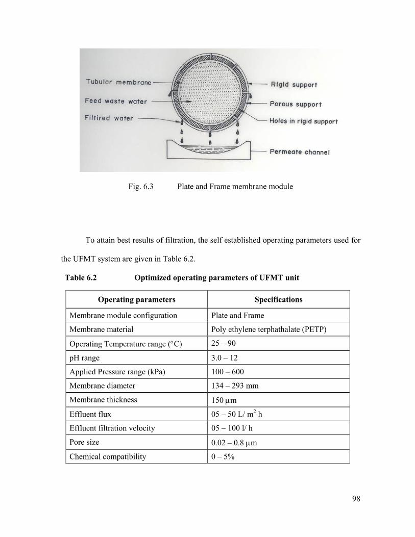
98
Fig. 6.3 Plate and Frame membrane module
To attain best results of filtration, the self established operating parameters used for
the UFMT system are given in Table 6.2.
Table 6.2 Optimized operating parameters of UFMT unit
Operating parameters Specifications
Membrane module configuration Plate and Frame
Membrane material Poly ethylene terphathalate (PETP)
Operating Temperature range (C) 25 – 90
pH range 3.0 – 12
Applied Pressure range (kPa) 100 – 600
Membrane diameter 134 – 293 mm
Membrane thickness 150 m
Effluent flux 05 – 50 L/ m2 h
Effluent filtration velocity 05 – 100 l/ h
Pore size 0.02 – 0.8 m
Chemical compatibility 0 – 5%

99
6.8.4. Membrane fouling
Due to prolong filtration, scaling and ultimate plugging of the membrane’s pores
may happen. The probability to foul a filter diverges with the nature of effluents. The
nature and amounts of fouling are reliant on various aspects such as quality of feed
effluent, brand/ materials of membranes, design and operating process conditions etc.
Three main types of fouling on a membrane are Chemical, Mechanical and Bio fouling.
Due to fouling, workload on membrane increases so much that the membrane is no longer
economically, practically and technically responsible. Chemical fouling arises due to the
build-up of gel, waxes, starches and metal hydroxides on the membrane surface. The
effluent fluxes can be restored by simple water washings or by chemical cleaning with
sodium peroxide or ammonium citrate rinses. Mechanical fouling is created by the
blockage of the feed spacer mesh due to particulates, which lead to an increased pressure
drop through the module, along with the reduction in effective membrane area. The extent
of fouling of the membranes can be evaluated by measuring the water flux of the
membranes. The water flux of a new membrane is in the region of 220 L/m2h yet after
about two month’s operation it drops to 90-110 L/m2h. Water flux can be decrease due to
following factors:
Membrane compaction
Chemical fouling of the membrane surface
Mechanical fouling of the feed spacer mesh
6.8.5. Membrane cleaning
There are a variety of cleaning techniques for the elimination of membrane fouling.
These procedures are air flushing, forward flushing, backward flushing, chemical cleaning

100
and various combinations of these methods. Ammonium citrate and sodium peroxide
solutions are commonly used for membrane’s cleaning purposes.
6.8.6. Membrane performance [153]
To check the membrane’s performance flux, effluent’s filtration velocity, time,
temperature, EC, pH, applied pressure, density and concentrations of the effluents with
their inter relationships are described here in sections 6.8.6.1 to 6.8.6.9.
6.8.6.1. Effect of Effluent’s Concentration on Flux
The concentration (%) of the industrial effluents and the flux (L/ m2 h) were
inversely proportional to each other. To study this relationship, actual industrial effluent
was diluted to prepare 10 solutions of different concentrations such as 10%, 20%, 30%,
40%, 50%, 60%, 70%, 80%, 90% and 100%. To speedup the filtration velocity, the
experiment was performed at 60 C. Three hyperbolic curves of the relationship for
ceramics, paper and textile effluents are shown in Fig. 6.4. In general, at very low
concentration (10%) of the effluent, the value of the flux is very high and it gradually
decreases with the increase in concentration (up to 100%).
0 20 4 0 6 0 80 1 00
4
8
12
16
20
24
6 0 oC
Flu
x (l
/m2 /h
)
C o n c e n tra tio n (% )
C e ra m ic s P a p e r T e x tile
Fig. 6.4 The effect of concentration (%) of the industrial effluents on the Flux (L/m2 h)

101
6.8.6.2. Effect of Effluent’s Concentration on Filtration Velocity
There was an inversely proportional relationship between the filtration velocity (L/
h) and % concentrations of the industrial effluents. Filtration velocity was measured by
using flowmeter. With the increase of concentration of the effluents i.e. from 10 to 100%,
there was a decrease in its filtration velocity. This trend was more pronounced in the case
of ceramics effluents and its filtration velocity was the lowest (15 – 30 ml/ min) among
other effluents even at 60 C, as shown in the Fig. 6. 5,
0 20 40 60 80 10010
20
30
40
50
60
70
60 0C
Filt
rati
on
Vel
oci
ty (
l/h)
C oncentration (% )
C e ram ics P ape r T e x tile
Fig.6. 5. The effect of Concentrations (%) of the industrial
effluents with their Filtration velocity (L/h)
6.8.6.3. Effect of Temperature on Flux
Fig. 6.6 illustrates the effects of temperature on the flux. Operation at high
temperature (0C) significantly increases the flux (L/ m2 h) and lowers the pumping cost.
Temperature – Flux curves for ceramics, paper and textile effluents are presented in the
figure. It indicates that there is the smallest flux range (3.0 – 6.5) for ceramics effluent, the
moderate flux range (4.0 – 11) for paper effluent and the highest flux range (5.0 – 15.8) for
textile effluent.

102
20 30 40 50 60 700
2
4
6
8
10
12
14
16
18
Flu
x (l
/m2 /h
)
T e m p e ra tu re (0C )
C e ra m ic s P a p e r T e x tile
Fig.6.6 The effect of Temperature (0C) on the Flux (L/m 2 h)
6.8.6.4. Effect of Temperature on Filtration Velocity
The parameters, filtration velocity (L/ h) and temperature (C) are directly
proportional to each other. The filtration velocity increases with increase in temperature.
The selected optimum temperatures are 25C, 30C, 40C, 50C, 60C and 70C. The three
straight lines with different slopes for ceramics, paper and textile effluents are shown in
Fig. 6.7. The textile effluent has the highest filtration velocity (78 L/ h). The paper effluent
has the moderate (48 L/ h) while the ceramics effluent has the minimum filtration velocity
(21 L/ h).
20 30 40 50 60 7010
20
30
40
50
60
70
80
Filt
rati
on
Vel
oci
ty (
l/h)
T em p e ra tu re (oC )
C e ra m ic s P a p e r T e x tile
Fig. 6.7 The effect of Temperature (C) on the Filtration velocity (L/h)

103
6.8.6.5. Effect of Time on Electrical Conductivity
The effect of time (h) on the electrical conductivity (mS/L) during the filtration of
effluents at 30 C is shown in Fig. 6.8. With the passage of time, due to the removal of
electrolytes from the effluents, the electrical conductivity (EC) decreases. For the
measurements of EC values in the effluents, 712 Conducto-meter (Metrohm) was used. Its
accuracy range was 0.01. The unit of EC is milli Siemens per centimeter (mS cm-1) or
milli ohms per centimeter (m mhos cm-1). The figure indicates that there is a very sharp
decrease in EC with in 5 hours during the filtration process. After that, steady state lines are
obtained for all the effluents.
0 10 20 30 40 505
10
15
20
25
30
35
4030 oC
Co
nd
uct
ivit
y (m
S/l)
Time (h)
Ceramics Paper Textile
Fig. 6.8 The effect of Time (h) on the Electrical Conductivity (mS/L)
during the filtration
6.8.6.6. Effect of Time on Filtration Velocity
The effect of time (h) on the filtration velocity (L/ h) at 25 C is shown in Fig. 6.9.
It is clearly indicated by the figure that the filtration velocity of all the effluents retards
with time during the filtration process. It is due to the chocking/ clogging/ fouling of the
pores of the filtration membrane. The novelty of the UFMT unit is that the blocked
membrane can easily be re-used after proper cleaning with suitable chemical/ water.

104
0 1 0 20 3 0 40 5 00
1 0
2 0
3 0
4 0
5 0
6 0
7 0
8 0
2 5 oC
Filt
rati
on
Vel
oci
ty (
l/h)
T im e (h )
C e ra m ic s P a p e r T e x ti le
Fig. 6.9 The effect of Time (h) on the Filtration velocity (L/h)
6.8.6.7. Effect of Density on the Filtration Velocity
The parameters, density (g/ L) and filtration velocity (L/ h) were found inversely
proportional to each other. Density was measured through 25 ml capacity density bottle.
Dense effluents have low filtration velocity as shown in the Fig. 6.10. The density range
(1.02 – 1.05 gm/ ml) of ceramics effluents is the highest. So its maximum filtration velocity
is 20 L/ h only. While the textile effluent was least dense and its maximum filtration
velocity was more than 40 L/ h even at room temperature.
1 .0 0 1 .0 1 1 .0 2 1 .03 1 .04 1 .0 5
1 0
2 0
3 0
4 0
5 0
6 0
7 0
2 5 oC
Filt
rati
on
Vel
oci
ty (
l/h)
D e n s ity (g m /m l)
C e ra m ic s P a p e r T e x t ile
Fig. 6.10 The effect of Density (g/ L) on the Filtration velocity (L/h)

105
6.8.6.8. Effect of Pressure on the Filtration Velocity
The separation efficiency increases with increasing operating pressure and
decreases with increasing time. Monometer was used for the measurement of liquid
pressure. The responses of applied pressure (Kpa) and filtration velocity (L/ h) of the
industrial (ceramics, paper and textile) effluents are indicated in Fig. 6.11. Three parabolic
curves describe that even with the increase of pressure (from 100 Kpa to 500 Kpa), the
filtration velocity of the industrial effluents decreases gradually with the passage of time. It
was due to the blockage in the pores of the membrane after prolonged filtration. In case of
ceramics effluents, due to the presence of mud, the complete blockage of pores occurred
with in 500 minutes of filtration process.
100 200 300 400 50010
15
20
25
30
35
40
25 oC
Filt
rati
on
Vel
oci
ty (
l/h)
Pressure (KPa)
Ceramics Paper Textile
Fig. 6.11 The response of applied Pressure (Kpa) on the Filtration velocity (L/ h)

106
6.8.6.9. Effect of Flux
The membrane flux is a complex function of inlet pressure, filtration velocity,
effluent concentration, temperature and membrane fouling. The applied pressure and
temperature both are linearly dependent on the flux. The flux rates were in the range 15 –
220 liters of product per m2 of membrane area per hour (M/m2 h). The response of the flux
(L/m2 h) with the specific gravity of mentioned effluents, at 60 C is shown in Fig. 6.12.
For all the industrial effluents, the flux was inversely proportional to the specific gravity.
The slope line for textile effluent was very sharp as compared to other effluents. Moreover,
the trend of specific gravity for the effluents was
Ceramics > Pulp/ Paper > Textile/ Yarn
1 .0 0 1 .0 1 1 .0 2 1 .0 3 1 .0 40
5
10
15
20
25
60 oC
Flu
x (l
/m2 /h
)
S p ec ific G ravity
C e ra m ics P a p e r T e x tile
Fig. 6.12 The response of the Flux (L/m 2 h) with Specific gravity
6.9. Removal of Pollutants
UFMT system is very efficient for the treatment of industrial effluents. The
pollution parameters such as pH, Biochemical Oxygen Demand (BOD), Total Suspended
Solids (TSS), Total Dissolved Solids (TDS), oil/ grease/ fat, Turbidity etc, were easily

107
controlled with the help of such system. The pH of the feed and purified effluents remained
at the optimized value ≈ 10 for the removal of pollutants and purification of all effluents.
Moreover, the separation efficiency of dyes and chromate from the industrial effluents is
also illustrated. A comprehensive analysis of the textile/ yarn and pulp/ paper effluents for
pollution parameters along with their measured values of the pre & post filtration and their
comparison with the relevant standards is presented in the Tables 6.3 and 6.4 respectively.
Table 6.3 Pre and post filtration values, with standard deviations, of the pollutants along with their recommended values for the effluents of textile industry
Parameters of pollution
Measured Values (mg/l) NEQS Standard (mg/L)
World Bank Guidelines (mg/L)
US-EPA Standards (mg/L) Pre-
filtration Post filtration
BOD5 639 ± 45 132 ± 16 80 33 – 49 33 – 49
TSS 787 ± 62 156 ± 13 150 82 – 123 36 – 54
TDS 7938 ± 583 4739 ± 271 3,500 3,500 3000
pH 12.7 ± 1.0 10.9 ± 0.5 6 – 10 6 – 9 6 – 9
Conductivity (mS/l)
38 ± 1.2 21.7 ± 0.8 5 – 20 3 – 15 3 – 15
Temperature (C)
58 ± 1.1 25 ± 0.7 40 30 30
Turbidity (NTU)
59 ± 2.4 35 ± 1.8 10 – 30 7 – 27 3 – 27
Oil & Grease 131 ± 11.7 21 ± 2.9 10 10 6 – 8
Total Solids 8776 ± 569 4897 ± 364 5000 4000 4000

108
Table 6.4 The contamination levels with standard deviations, before and after the purification, for the effluents of pulp/paper/board industry along with their recommended values
Parameters of pollution
Measured Values (mg/l) NEQS Standard (mg/L)
World Bank Guidelines (mg/L)
US-EPA Standards (mg/L) Pre-
filtration Post filtration
BODs 2350 ± 115 630 ± 53 80 33 – 49 33 – 49
TSS 930 ± 70 280 ± 24 150 82 – 123 36 – 54
TDS 8236 ± 615 4640 ± 367 3,500 3,500 3000
Temperature (C)
44 ± 1.0 25 ± 0.6 40 37 37
pH 12.1 ± 0.5 10.2 ± 0.4 6 – 10 6 – 9 6 – 9
Conductivity (mS/l)
56 ± 1.9 27 ± 0.9 5 – 20 3 – 15 3 – 15
Turbidity (NTU)
51 ± 2.3 37 ± 1.1 10 – 30 7 – 27 3 – 27
Oil & Grease 83 ± 4.6 16 ± 1.0 10 10 6 – 8
Total Solids 9166 ± 431 4920 ± 212 5000 4000 4000
6.9.1. Reduction of BOD
Biochemical Oxygen Demand (BOD)5 test measures the losses of dissolved oxygen
in the effluent, incubated over a period of 5 days, under standard conditions. The dyes
increase the BOD by consuming dissolved oxygen and thus upset the biological activities
in the aquatic environment. The reduction values of BOD by this method were presented in
Table 6.3 for the effluents of textile/ yarn and in Table 6.4 for the effluents of pulp/ paper
industries.

109
6.9.2. Separation of TSS
Effluents of textile/ yarn and pulp/ paper industries were rich with the suspended
solids. There were dense pollutants of different contaminations, which float with the
effluents. The UFMT system was equipped with a grid and membrane, which separated the
suspended solids from the effluents. Separation of Total Suspended Solids (TSS) from the
effluents of textile/ yarn and pulp/ paper was reported in Table 6.3 and 6.4 respectively. For
TSS, there was a significant change in pre and post filtration effluents.
6.9.3. Elimination of oil and grease
Oil and grease were produced during the treatment of raw materials and their
washings. Such pollutants could block the sewer lines when they passed along with the
effluents. Moreover, they prevent the transfer of oxygen from atmosphere to the ground
water bodies, which retards the aquatic life. UFMT system was very successful for the
elimination of oil and grease from the effluents. FTIR spectrometer was used for the
measurements of oil and grease. As proved by FTIR spectrometric results, the quantitative
eliminations of these pollutants were indicated in Table 6.3 for the effluents of textile/ yarn
and in Table 6.4 for the effluents of pulp/ paper industry.
6.9.4. Removal of turbidity
The effluents of textile/ yarn and pulp/ paper were dense in turbidity. The turbidity
was measured by Micro-100 Turbidimeter (HF Scientific Inc.). The meter showed very
high values in the pre-filtration effluents and removal of turbidity was very pronounced in
the post filtration effluents. The phenomenon was illustrated in Tables 6.3 & 6.4 for the
effluents of textile/ yarn and of pulp/ paper industry respectively.

110
6.9.5. Retardation of TDS
High concentrations of Total Dissolved Solids (TDS) were mentioned in Table 6.3
for the effluents of textile/ yarn and in Table 6.4 for the effluents of pulp/ paper industry.
The treated effluents (post filtration with membrane) were checked by TDS meter, which
declared that the readings for such pollutants were significantly reduced in them.
6.9.6. Extraction of Dyes
Rhodamine-B, Metomega chrome orange GL, Methylene blue etc, dyes are widely
used in various industries for colouring purposes [154-156] and their discharge in to water
bodies causes environmental pollution. There are so many significant hazards of such dyes
because they are toxic in nature. Mostly they cause body pain, ulceration of skin,
hemorrhage, acute diarrhea, kidney damage and a loss of bone marrow leading to anemia.
Effluents from industries such as carpet manufacturing, dyeing, pulp/ paper, tanneries/
leather and textile/ yarn, were rich in colour. The quantitative extraction of almost all
colour/ dyes from the industrial effluents was checked by the measurement of % absorption
of light through UV-Visible Spectrophotometer. Fig. 6.13 illustrates the intensity of colour
differences for pre and post filtration of ceramics, paper and textile effluents at λmax 665 nm
for Methylene Blue and λmax 544 nm for Rhodamine-B dyes respectively. It is indicated
from the figure that the textile effluent is the densest in colour so its values for %
absorption are also very high as compare to others.

111
0 20 40 60 80 1000
1 5
3 0
4 5
6 0
7 5
9 0
2 5 oC
Ab
sorb
ance
(%
)C o n c e n tra tio n (% )
C - P re C - P o s t P - P re P - P o s t T - P re T - P o s t
Fig. 6.13 Pre and post filtration curves for the extraction of dyes/
coloured materials from the industrial effluents
6.9.7. Removal of Chromate
The %removal of chromate ions has been reported by various scientists [157-160].
PETP membrane was used first time from different concentrations (%) of industrial
effluent on various applied pressures (Kpa) at 70 C and 10 pH is shown in Fig. 6.14. It
was observed that the removal rate of chromate was highly dependent on the pH of the feed
effluents. With increase in pressure, the % removal efficiency for chromate decreases.
While with increase in effluent’s concentration, the % removal efficiency for chromate also
increases. The plots also demonstrate the efficiency of the UFMT unit in removing
chromate from contaminated effluent stream at applied pressures.
100 200 300 400 5000
20
40
60
80
100
70 0C pH 10
% R
emova
l of Chro
mat
e
Pressure (PKa)
Effluent 20% Effluent 40% Effluent 60% Effluent 80% Effluent 100%
Fig. 6. 14 Removal of chromate (%) from different concentrations (%)
of effluents at various applied pressures (Kpa)

112
6.10. Sweet peanut husk, a potential scavenger
The presence of heavy toxic metals in industrial effluents is a severe pollution
problem. Therefore, the need to monitor, control and remove the toxic metal ions and
hazardous organic substances from industrial effluents [161-168] has focused the attention
for their efficient and cost effective treatment. The available methods for the removal of
toxic metals are expensive and time consuming. Many agricultural waste materials utilize
as natural ion exchanger/ scavenger/ adsorbent for the treatment of industrial effluents yet,
all have their own advantages and limitations.
In the present research, sweet peanut husk has been used as an adsorbent for the
removal of arsenic (As), chromium (Cr) and Iron (Fe) from the industrial effluents.
6.10.1. Low cost materials
Some economical materials have been utilized on routine bases for the separation of
toxic metals, even with very low concentrations, from the industrial effluents which are
activated charcoal, maize combs, rice husk, onion skin, coconut husk, bagasse, Barks,
natural clay, mineral mixture, foam, wool, etc. These are not ultimate waste materials
because they can further be used in the preparation/ synthesis of various other useful
products such as sofa cushion, foot mat, pulp/ paper, pillows and heat. However, from
industrial point of view, peanut husk has not any significant value.
6.10.2. Sweet peanut husk
Raw peanut skin cannot be used as a good natural absorbent due to its two major
disadvantages. First, on contact with water, there is a leaching of reddish colour into the
solutions. Second, on prolonged contact with water, peanut skin tends to disintegrate. On
the other hand, the sweet peanut husk has an enough potential to be used as a scavenger for

113
the economic and effective removal of heavy metal ions as arsenic (As), iron (Fe) and
chromium (Cr) from the industrial effluents. Peanut husk is an inexpensive natural organic
waste material because it has no significant industrial utility. It is easily and abundantly
available in nature. It can be retained in water for more than three months without any
deterioration. Its absorption tendency for toxic elements is also appreciable. Moreover, it is
resistant to some extent against heat, temperature variations, pH, mechanical stress and
chemical corrosion. The binding capacity of peanut husk is quite high (1meq of metal/ g of
the substrate) for Cr, As and Fe ions and is competitive with many synthetic ion-
exchangers. The reaction rate is reasonably fast requiring short contact time.
6.10.3. Purification/ preparation of peanut husk’s material
Sweet peanut husk was collected from various sources. It was physically purified to
remove bagasse, small pieces of papers/ cotton, stones etc. Then it was thoroughly washed
with tape water to remove all dust/ attached unwanted environmental contaminations and
was oven dried at 70 C till constant weight. It was then ground and sieved up to required
mesh sizes (50-100 mm) to obtain homogenized material. It was done in order to increase
its surface area and to reduce wall effects in small packed columns, which were used in
laboratory continuous processes. After proper grading, all prepared samples were packed in
suitable containers and were stored in clean/ dry places at room temperature.
6.10.4. Solutions preparation
According to the requirements, the following solutions have been prepared from the
standard purified chemicals. All the reagents used were of analytical grades. Distilled and
deionized water was used through out the experiment.

114
6.10.4.1. Buffer solutions
Buffer solutions of twelve different strengths (1 – 12 pH) have been prepared to
maintain the acidic strength of adsorbent during column chromatography. The preparation
scheme is given in the following Table 6.5.
Table 6.5 Preparation of buffer solutions (pH 1-12) [6]
pH Buffer mixtures
1 0.1 M HCl
2 250 ml 0.2 M KCl + 53 ml 0.2 M HCl (up to 1L)
2 5.26 g NaCl + 100 ml 0.1 M HCl (up to 1L)
3 500 ml 0.036 M HCl + 7.35 g KH Phthalate (up to 1L)
4 10.2 g anhydrous KH Phthalate [KHC8H4O4] (up to 1L)
5 20.4 g KH Phthalate + 3.73 g KCl + 50 ml 1 M KOH (up to 1L)
6 250 ml 0.2 M KH Phthalate + 227 ml 0.2 M NaOH (up to 1L)
7 2.72 g KH Phthalate + 4.26 g Na2PO4 + 1.16 g NaCl (up to 1L)
8 250 ml 0.2 M KH2PO4 + 234 ml 0.2 M NaOH (up to 1L)
8.2 3.1 g Boric acid + 3.73 g KCl + 29.5 ml 0.2 M NaOH (up to 1L)
9 3.81 g Borax [Na2B4O7.10H2O] + 1.7 g NaCl (up to 1L)
10 250 ml 0.2 M H3BO3 + 250 ml 0.2 M KCl + 220 ml 0.2 M NaOH (up to 1L)
12 1.28 g Ca(OH)2 + 1.06 g NaCl (up to 1L)
6.10.4.2. Stock/ Standard solutions of Acids
Standard stock solutions of 1 M concentration of HCl, HNO3 and H2SO4 were
prepared through standard procedure. The solutions of 0.1, 0.01 and 0.001 M strengths
were prepared from the stock solutions of the respective acids by dilution technique
6.10.4.3. Standard solution of Arsenic
Stock solution of arsenic (450 ppm) was prepared according to the prescribed
standard procedure. Analytical grade arsenic oxide (As2O3) of 0.2981 g was dissolved

115
within a minimum amount of 0.01 M HCl. The solution was warmed for rapid dissolution
of oxide. The resultant solution was then diluted up to one liter (1L) with distilled water.
6.10.4.4. Standard solution of Chromium
Stock solution of chromium (1000 mg/ L) was prepared according to the prescribed
standard procedure. One-gram (1g) spec-pure chromium metal was dissolved with in a
minimum amount of 0.01 M HCl. The solution was warmed for rapid dissolution of metal.
The resultant solution was then diluted up to one liter (1L) with distilled water.
6.10.4.5. Standard solution of Iron
Stock solution of iron (499 ppm) was prepared according to the prescribed standard
procedure. Analytical grade ferrous sulphate (FeSO4. 7H2O) of 2.48 g was dissolved in de-
ionized water. The solution was warmed for rapid dissolution of the compound. The
resultant solution was then made up to one liter (1L) with distilled water.
6.10.5. Physico-chemical parameters to optimize the conditions
The following essential parameters, leading to maximum absorption, have been
optimized according to the experimental conditions and applied to check the efficiency of
the sweet peanut husk to remove the concerned metal ions from the industrial effluents.
i. Appropriate electrolyte ii. Shaking/ mixing time
iii. Concentration of absorbent iv. Concentration of absorbate v. Temperature range
vi. pH range vii. Mesh size of absorbent
viii. Column bed length
6.10.6. Adsorption process (Experimental setup)
The amount of adsorbent was affected with the efficiency of the adsorption. 1mm-
screened material (peanut husk) was used to optimize adsorption process. 1.5 cm inner

116
diameter (ID) and 50 cm long glass tubes with stopper/ nozzle were used as columns. Dry
adsorbent was poured in to the column and the column was tapped very gently to promote
even distribution of packing. In this way, 10 cm long uniform beds of adsorbent, in each
column, were prepared to perform column chromatography. The packing density was
approximately 0.15g/ cm2. Glass wool was used as plugging agent, on the top and bottom
of the packing bed, to prevent the adsorbent particles from floating/ leaking/ separating etc.
It was then pregnant with 500 ml 1 pH buffer solution up to the saturation stage. The whole
experiment was performed at room temperature.
Activated samples were prepared according to the prescribed procedures. The dry
solid arsenic (As) sample was irradiated for intermediate time interval as 10 – 35 minutes.
Similarly, dry solid chromium (Cr) and iron (Fe) samples were irradiated for 300 minutes
in Pakistan Research Reactor (PARR) at a thermal neutron flux of 4.5 x 10¹³ n cm-2 sec-1.
Three columns with bed size 9.5, 8.5 and 7.5 cm were used for each experiment. In first
experiment, 5.0 ml activated arsenic (As) solution was loaded in each column on the un-
modified peanut husk bed. Flow of metal ion solutions, through the column, was by gravity
and was controlled by the stopper valve. The loading capacity of the peanut husk for metal
ions under the optimal conditions was 23.7 to 45 gram metal ions per kilogram husk. Then
the elution of activated arsenic (As) solution was started with 0.001, 0.01 and 0.1 M HCl
respectively, from all three columns. During the elution, 5 ml acid solution was added from
the top and collected from the bottom to check the activity through counter. This step was
repeated for several times until a clean solution with out any activity was obtained from the
bottom of each column. The peanut husk bed was washed thoroughly with fresh water to
reuse it. The same experiment of arsenic was repeated with the activated solutions of

117
chromium (Cr) and iron (Fe) one by one. Above 99% adsorption was obtained using the
peanut husk. The error was within 3%.
For the treatment of industrial effluents, a pre-filter such as wire gauze was used in
front of the peanut husk trap to stop the sludge/ floating particles which could block the
trap and decrease the flow rate of the effluents.
6.10.7. Analysis of Industrial Effluents
Effluents of textile/ yarn, pulp/ paper and ceramics industries, collected from
Faisalabad and Gujranwala areas, were analyzed to evaluate the toxicity of industrial
pollution. In this regard, more than twenty-six trace elements including essential, non-
essential, toxic and rare earth elements were determined qualitatively/ quantitatively
through NAA and AAS techniques. Among them, the amounts of arsenic (As), chromium
(Cr) and iron (Fe) were found to be above the recommended permissible levels. So they
were removed from the effluents through adsorption by peanut husk. Some salient features
of these elements are described below.
6.10.7.1. Chromium (Cr)
Chromium is a naturally occurring element found in rocks, animals, plants, soil,
volcanic dust and gasses. Its main contributing industries are the mining, metal plating,
chemical pigments, leather tanning and textile. Its dietary sources are meat, liver, brewer’s
yeast, whole grain nuts and cheese. Chromium is widely distributed in the body tissues. Its
physiological importance is for the regulation of blood sugar. It is essential for the
maintenance of normal glucose/ insulin and lipid/ protein/ amino-acid metabolism. The
biological effects of chromium depend on its valency i.e. in the trivalent form chromium is
an essential element while in the hexavalent form it is carcinogenic. The deficiency of this

118
element produces hyperglycemia, hypo-cholestermia, diabetes, weight loss, growth
retardation and cardiovascular disease. Chromium at higher concentration levels is
injurious to health because it induces muco-dermal ulceration, lung cancer, liver/ kidney
damage and allergic dermatitis of the skin.
6.10.7.2. Arsenic (As)
Arsenic is present in atmosphere, minerals, smelting of ores, various biological
substrates, sea and fresh water. Arsenic is widely distributed in human tissues, hair, skin
and nails. The accumulation of arsenic can damage the kidney, liver, spleen and heart.
Absorption of this element above the tolerance limit results in toxicity causing anorexia,
nausea, weight loss, vomiting, diarrhea, burning of mouth and throat. A chronic exposure
results in hepatic toxicity, weakness, muscular aching, gastrointestinal disorder,
pigmentation in finger and nail, drowsiness and headache. For human beings, arsenic has a
carcinogenic effect on health. The WHO recommends a limit of 0.05mg As/ kg body
weight in the daily ingestion of food. The recommendation of WHO for drinking water was
up to 20g/L. The normal body burden of adults is 10-20 mg for arsenic.
6.10.7.3. IRON (Fe)
Iron is one of the essential nutrients for human health and life. Iron constitutes
5% of the earth’s crust so it is one of the most abundant metallic elements. The biological
significance of iron is derived largely from its ability to undergo reversible oxidation-
reduction reactions. Activity of a number of metallo-enzymes and metallo-proteins is
dependent on this element. Iron is a necessary component of many important body
constituents, e.g. hemoglobin, myo-globin, enzymes etc., which have essential roles in the
utilization of oxygen and for energy requirements in cells. Fe is also involved in CO2 –

119
transport and in maintaining the proper physiological pH. The need for iron in the human
diet varies greatly at different ages and under different circumstances. Iron deficiency
causes paleness of skin leading to anemia and reduced blood hemoglobin concentration and
muscle exertion, reduced physical activity and palpitation.
6.10.8. Effect of pH
The influence of pH (1-12) is critical because it regulates the release of free metal
ions from bound chemical forms in the industrial effluents. The pH also controls the
adsorption of the metal ions on the peanut husk. The pH of effluents was measured with the
help of a pH meter # 8520 (Hanna). Its accuracy range was 0.01. A decrease of sorption
from pH 5.0 was due to the formation of colloidal/ hydroxide species, which did not
undergo complete sedimentation. The pH factor also affected the surface charge of the
adsorbent, degree of the ionization and speciation of the adsorbate. The best results were
obtained for the removal of arsenic (As), chromium (Cr) and iron (Fe) ions at pH 5.0 as
shown in Fig. 6.15.

120
0 2 4 6 8 10
0
20
40
60
80
100
% A
dso
rpti
on
pH
Cr As Fe
Fig. 6.15 Response of pH vs space of Cr, As and Fe on Peanut husk
6.10.9. Effect of acid concentrations
The effect of acid concentration is important for the assessment of the metal
adsorption process. Therefore, the adsorption behaviour of metal ions was measured in
mineral acids (HCl, HNO3 & H2SO4) having concentration range from 0.001 to 1.0 M. The
maximum adsorption of metal ions occurred at the acid concentration of 0.01 in all the
acids used in the present study, which gradually decreased with the increase of acidic
concentrations. The % adsorptions of arsenic, chromium and iron metal ions on the peanut
husk, with various concentrations of mineral acids, are illustrated in Figures 6.16, 6.17 and
6.18 respectively.

121
0.00 0.02 0.04 0.06 0.08 0.10
80
82
84
86
88
90
92
94
96
98
100
HCl HNO3
H2SO4
% A
dso
rpti
on
of
As
Acid Conc. (M)
Fig. 6.16 Behaviour of % adsorption of Arsenic on the Peanut husk with various concentrations of mineral acids
0.00 0.02 0.04 0.06 0.08 0.10
0
10
20
30
40
50
60
70
80
HCl HNO3
H2SO4% A
dso
rpti
on
of
Cr
Acid Conc. (M)
Fig.6.17 Behaviour of % adsorption of Chromium on the Peanut husk with
various concentrations of mineral acids

122
0.00 0.02 0.04 0.06 0.08 0.105
10
15
20
25
30
35
HCl HNO3
H2SO4
% A
dso
rpti
on
of
Fe
Acid Conc. (M)
Fig. 6.18 Behaviour of % adsorption of Iron on the Peanut husk with various
concentrations of mineral acids
6.10.10. % Removal of concerned metals
The concerned metal ions have been removed up to 99% from the industrial
effluents by the use of peanut husk. The maximum removal of Cr, As and Fe metal ions
was achieved at 0.01 molar concentration of HCl solution as shown in Fig. 6.19. The
behaviour/ pattern of all the metal ions were somewhat similar to each other. The metal
removal efficiency was very low at high acidic concentrations.
-3 -2 -1 0 1
20
40
60
80
100
% M
etal
Rem
ove
d
Log 10 x (Molar Conc.)
As Cr Fe
Fig. 6.19 % Removal of Cr, As and Fe metal ions from the industrial
effluents by Peanut husk

123
CHAPTER-7
7. DISCUSSION
The concentrations of 24-30 major, minor and trace elements in each part of the
vegetables/ crops were evaluated on dry weight basis and the statistical results, as the
averages of at least five determinations with standard deviations around mean values, are
given in the Tables 6.1 to 6.12. The concentrations of some preferred trace elements have
been plotted in the Figures 7.1 to 7.41 to graphically display their concentration pattern in
effluents, cereal, vegetables and soils. The concentration values are plotted in the log scale
in order to combat the variations of concentrations due to large differences in their ranges
and to make the results compatible. On the basis of epidemiological, clinical, pathological
and experimental evidence, it is established that trace elements play curative and preventive
roles in combating diseases while the intake of toxic elements, above the tolerence limit,
are health injurious and may create the impairment in the vital organs of the body. The
normal biological functions adversely affected due to the excess accumulation or
deficiency of trace elements in the human body Therefore, a balance amount of such
constituents is required for the maintenance of good health and optimum health
performance. Mechanized forming, use of artificial fertilizers, spray of harmful chemicals,
irrigation with industrial effluents etc are the major causes to induce contamination in
vegetarian food. The efficient control and management of the environmental burden caused
by the industrial pollution has become an issue of human health [169-172]. The present
research offers baseline values for toxic and essential elements in diverse varieties of crops
and vegetables cultivated with the industrial effluents, which will be helpful to monitor the
changes in trace element contents of these items in future.

124
7.1. Quality Assurance for the Results
All the procedures of the chemical analysis were utilized with the highest
precision to ensure the validity/ reliability of the method and integrity of the results.
Biological matrices were usually difficult to analyze due to low concentrations of some
important trace elements. For accurate analysis, extensive care was taken during research
and sources of error were minimized. To achieve best results, following steps were used:
1. Representative and uncontaminated samples were composed. Addition or loss
during sample preparation/ storage was avoided.
2. Every analytical parameter e.g. irradiation/ decay time, sample weight, irradiation
site in the reactor etc. for NAA was optimized both for the sample and CRMs.
3. Gamma spectrometric measurements and subsequent spectrum analysis were
vigilantly performed. Spectral interferences were also taken into account.
By analyzing CRMs of similar matrix compositions with a particular set of
samples, the accuracy of overall analytical procedure was examined, which was the most
direct and reliable method for quality assurance. For a sample, the choice of particular
reference materials was made on the basis of .the maximum matrix match, maximum
number of certified elements available and the comparable analyte concentrations. The
values of present research were fairly in good agreement with the certified/ reference
values of used different biological CRMs, as shown (section 6.1 Validation of methodology
for NAA technique) in the Table 6.1 and geological CRMs, as shown (section 6.2
Validation of methodology for AAS technique) in the Table 6.2.
To make sure the analytical quality control, Z-score method of self-assessment was
adopted to assess the difference between the measured and the certified values. IAEA
applies this method in proficiency tests to check and assess the measured results. Z score,

125
which helped to recognize systematic errors and to optimize the data quality, was utilized
according to the following formula:
(X1 – Xa) Z – Score = ________________ Sb
Where X1= arithmetic mean of reported value Xa = arithmetic mean of certified value Sb = target standard deviation
The Z-score values for all the elements in CRMs were measured with standard
procedure. The calculated Z score values were plotted against trace element as shown in
figures 7.1, 7.2 & 7.3 for IAEA-336, IAEA-SL-1 and IAEA-S-7 respectively. The positive
score shows higher than the actual value and negative score denotes lower than the actual
value. The reliability of the results was satisfactory for the values +2 Z -2. The plots
clearly pointed out that almost all the analyzed elements for this research were present
within the permitted limits i.e. the upper warning limit (UWL) with positive Z-score values
of less than +2 and lower warning limit (LWL) with negative Z-score of –2 values.
2 4 6 8 1 0 1 2 1 4
- 3
- 2
- 1
0
1
2
3
Z n
T h
S r
S eS bN a
M nK
F e
C u
C r
C o
C l
B r
A s
L W L
L C L
U W L
U C L
Z -
Sco
re
E l e m e n t s
Fig. 7.1 Z – Score values for trace elements in SRM IAEA-336 (Lichen)

126
2 4 6 8 1 0 1 2 1 4
- 3
- 2
- 1
0
1
2
3
B r
T h
M n
Z nS r
C o
S e
F e
C lS bC u
K
A s
C r
N a
L C L
L W L
U W L
U C L
Z -
Sco
re
E l e m e n t s
Fig. 7.2 Z – Score values for trace elements in SRM IAEA-SL 1 (Lake Sediment)
2 4 6 8 1 0 1 2 1 4
- 3
- 2
- 1
0
1
2
3
C o
T hC uK
S e
N aB r
C r
F e
Z n
A s
M n
R b
S r
S b
L C L
L W L
U W L
U C L
Z -
Sco
re
E l e m e n t s
Fig. 7.3 Z – Score values for trace elements in SRM IAEA-S 7 (Soil)
Solutions for the interferences in Gamma peaks
A majority of the elements were resolute without any spectral interference of
gamma peaks for sample analysis through NAA technique with a few exemptions. The
photo-peak of 46Sc at 1120 keV could not be resolved from 1115 keV of 65Zn due to the
comparatively higher amount of zinc in the matrix. To solve this trouble, the data for
another peak of 46Sc at 889.3 keV with -abundance of 100% was considered to calculate
the concentration of scandium while the zinc concentration was computed using 1115 keV
γ-peak subtracting the contribution of 1120 keV from 46Se. Interference of 134Cs at 604.7

127
keV (98%) peak was recorded with full intensity peak of 124Sb at 602.7 keV (98.1%). The
concentration of antimony was evaluated by using less intense, interference free peak at
1691.0 KeV (50%) with long counting times. Cesium-134 concentration was estimated via
interference free peak at 795.8 keV (89%) instead of more intense peak at 604.7 keV.
The high profusion photo-peak of 140La at 1596.5 keV, which is free from
interference, was utilized for the calculation of lanthanum. The other peak at 487 keV
cannot be utilized due to interference from 47Ca. The photo-peak of 141Ce at 145.5 keV was
incorporated for the determination of cerium. However, in certain samples containing
significant amount of iron, the peak of 141Ce was not fully resolved from 142.5 keV peak of
59Fe. In such cases the two peaks were integrated together and the contribution of 142.5
keV peak, as estimated from 1292 keV peak of 59Fe was subtracted from it. Large quantity
photo-peak of 155Sm at 104.2 keV, which is free from interference, was incorporated for the
calculation of samarium. 152Eu has a number of peaks however; only high abundance peak
at 1408 keV was utilized, which was interference free. The photo-peaks of 160Tb at 1178
keV and 299 keV were utilized for the estimation of terbium as other high abundance peaks
had interferences. The second highest quantitative peak of 175Yb at 283 keV, which is
interference free, was used. It was difficult to resolve 396 keV peak from that of 152Eu.
Ytterbium was also determined using 308 keV peak of 169Yb. The values obtained via the
two routes were in very good agreement with each other.
In the same way the single photo-peak of 203Hg was at 279.2 keV (81.5%) and
75Se had three photo-peaks with energies 136 keV (58%), 264.7 keV (58.5%) and 279.5
keV (25%). The photo-peak of 75Se at 279.5 keV interfered with the photo-peak of 203Hg.
This problem was trounced by calculating the concentration of selenium from the non-

128
interfering peak at 264.7 keV. The peak area under the 264.7 keV of 75Se was multiplied by
the correction factor of 0.4 to evaluate the contribution of selenium to peak area of the
279.5 keV peak. The correction factor was derived from the abundances of these two
radionuclides along with the minor variation in the efficiency of the detector at the two -
peaks used. The calculated area was then subtracted from the total peak area corresponding
to the 279.3 keV peak to discover upon the actual corrected peak area due to mercury. This
value was then incorporated to find the concentration of 203 Hg at 279.2 keV.
7.3. Industrial Effluents
All industrial effluents were collected from the textile/ yarn, pulp/ paper and
ceramics industries situated in Faisalabad and Gujranwala municipal areas. Ceramics
industry was situated within Gujranwala area only. The effluents were analyzed through
NAA and AAS techniques for the quantitative estimation of trace elements. Their detailed
results (section 6.3 Trace elemental contents in the effluents) for each industry have been
presented in Tables 6.3 a, b & c respectively.
7.3.1. Physico-Chemical analysis of Effluents
Physico-Chemical analysis indicates the nature of the industrial effluents, which
is very useful and important factor for the prediction and estimation of different
parameters. The nature of effluents influences the soil and ultimately involves the quality
and quantity of the crops because industrial effluents cultivate a large area of soil in
Pakistan. Tables 6.4 a, b & c represented the results of physico-chemical analysis for the
effluents of 325 textile, 111 pulp and 118 ceramics industries respectively. Different
physical/ chemical parameters such as colour, volume/ dry weight of all collected effluents,
temperature, pH, density, electrical conductivity (EC), total dissolved solids (TDS),

129
specific gravity, turbidity, etc were measured through appropriate analytical techniques/
instruments as mentioned in the sections 5.8.6.1 to 5.8.6.9 Comparisons of different
parameters for the physico-chemical analysis of the effluents of textile, pulp and ceramics
industries are presented in the Table 7.1.
Table 7.1 A comparison of physico-chemical parameters among the effluents of textile, pulp and ceramics industries along with the NEQS values
Industries/ Parameters
Textile/ Yarn Pulp/ Paper Ceramics NEQC Standards
Temperature (0C) 56.0 60.9 41.0 45.9 26.0 30.0 40
pH 9.10 10.95 6.1 10.8 8.10 9.90 6 - 10
EC (mS/ cm) 10 35 15 40 7.25 15.50 5 - 20
Weight of dry samples (g/l)
0.444 1.311 1.095 14.40 10.029 23.280
TDS (ppm) 4187 7826 4789 9626 302 618 3,500
Turbidity (NTU) 16 45 25 59 8.30 34.65 10 - 30
Parameter pH is a vital factor especially for the uptake of micronutrients from
the soil by a plant. Electrical conductivity (EC) is the indicator of the presence of alkali and
alkaline earth metals in the samples. Sodium contents determine the salinity of the soil. The
plant growth is depressed with the increase in sodium contents in the soil, while it is
enhanced with the presence of high concentration of Ca and Mg salts. The physico-
chemical analysis of all effluents revealed that the values of temperature and pH were
higher for the effluent of textile industry as compared to the effluents of rest of the
industries. The ranges of turbidity, EC and TDS for the effluents of pulp were higher and
for the effluents of ceramics, all values were low except the dry weight of the samples.

130
7.3.2. Effluents of Textile/ Yarn Industry
The 325 effluent samples were collected from different textile/ yarn industries
situated in Faisalabad and Gujranwala areas. In each sample, 27 trace, essential, non-
essential, toxic and rare earth elements were measured as shown in Table 6.3.a (section
6.3). Samples with similar results were arranged in one group. The comparison of results
for six groups from textile industries shows that the elemental concentrations of Cs, K &
Zn is higher in the effluents of group # 503. Cl, Co, Lu & Sm elemental concentrations are
higher in the group # 510. The elemental concentrations of Al, As, Cr, Cu, Fe, Mn, Na, Tb,
Th & Zr are higher in the effluents from group # 520. Only Hf & Sb are high in the group #
529. In the group # 544, the concentrations of Ba, Br, Ca, Eu, Mg & Sc are higher. The
elemental concentrations of Ce, Rb, Se, Ta & Yb are higher in the effluents of group # 549.
A s B r C l C o S b S e T h
0 . 1
1
1 0
Co
nce
ntr
atio
ns
(pp
m)
E l e m e n t s
T 5 0 3 T 5 1 0 T 5 2 0 T 5 2 9 T 5 4 4 T 5 4 9
Fig. 7.4 Comparison of different effluents from textile industry
The Fig. 7.4 shows that the concentration of Cl (19100-12440) is very high in all
textile effluents. The concentrations of Br (75-52), Th (7.6-3.4), Co (8.5-2.2) & As (49.1-
15.2) are also on higher side, while the concentrations of Se (0.48-0.1) & Sb (1.89-1.24) are
in low quantities. The effluent of group # 520 is the worst among all other textile industries
due to the presence of high concentrations of all toxic elements.

131
7.3.3. Effluents of Pulp/ Paper Industry
The effluent samples were collected from 139 different pulp/ paper industries
located in the vicinities of Faisalabad and Gujranwala areas. In each sample 26 trace,
essential, non-essential, toxic and rare earth elements were determined as shown in Table
6.3.b (section 6.3). On the basis of variations in the concentration ranges, some groups of
similar results were made and were given them numbers as P-312, P-320, P-338 etc. The
comparison of results for randomly selected six groups shows that the elemental
concentrations of Co & Cs are higher in the effluents of group # 312. Fe, Ce, Zr, Se, Yb K,
& Cl elemental concentrations are higher in the group # 313. The elemental concentrations
of Mg, Ca, Rb, Lu & Th are higher in the effluents from group # 320. The elemental
contents of Al, Sm, Br & Zn are higher in the group # 324. In the group # 335, the
concentrations of Eu, Sc, As, Na, Hf, V, Sb, Ta & La are high. The elemental
concentrations of Cr & Mn are high in the effluents of group # 338.
A s B r C l C o S b S e T h
0 . 1
1
1 0
Co
nce
ntr
atio
ns
(pp
m)
E l e m e n t s
P 3 1 2 P 3 1 3 P 3 2 0 P 3 2 4 P 3 3 5 P 3 3 8
Fig. 7.5 Comparison of different effluents from pulp industry
This Figure indicates that As (31-15 μg/g) & Br (52-18 μg/g) concentrations are
on higher side while the concentrations of Co (4.7-1.6 μg/g), Sb (0.49-0.22 μg/g), Th (5.9-
1.8 μg/g) and Se (0.42-0.12 μg/g) are on lower side in all the pulp effluents. The

132
concentration of chlorine (19960-6480 μg/g) is as usual high for all effluents. It has been
revealed from the obtained results and is also indicated in the Fig. 7.5 that the effluent of
group # 335 is the worst among all other pulp industries due to the presence of high
concentration of all toxic elements.
7.3.4. Effluents of Ceramics Industry
The effluent samples were collected from 118 different ceramics industries
located in the vicinity of Gujranwala. There was no ceramics industry situated in the
vicinities of Faisalabad areas. As shown in Table 6.3.c (section 6.3), in each sample, 27
trace, essential, non-essential, toxic and rare earth elements have been measured. The
comparison of results of randomly selected six groups shows that the elemental
concentrations of As, Cr, Mg & Na are higher in the effluents of group # 204. Al, Ba, Co,
K, La, Sc & V elemental concentrations are higher in the group # 206. The elemental
concentrations of Mn, Br, Zn, Sb, Sm, Eu & Zr are higher in the effluents of group # 207.
The elemental concentrations of Cl, Cs, Ta, Ti & Yb are higher in the effluents of group #
209. In the group # 212, the concentrations of Ca, Th, Se & Lu are higher. Only Fe, Ce, Hf
& Rb are higher in the group # 215.
A s B r C l C o S b S e T h
0 . 1
1
1 0
Co
nce
ntr
atio
ns
(pp
m)
E l e m e n t s
C 2 0 4 C 2 0 6 C 2 0 7 C 2 0 9 C 2 1 2 C 2 1 5
Fig. 7.6 Comparison of different effluents from ceramics industry
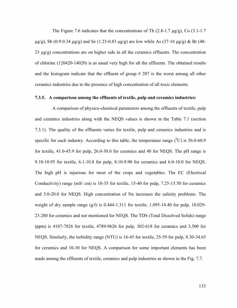
133
The Figure 7.6 indicates that the concentrations of Th (2.8-1.7 μg/g), Co (3.1-1.7
μg/g), Sb (0.9-0.34 μg/g) and Se (1.23-0.83 μg/g) are low while As (37-16 μg/g) & Br (48-
23 μg/g) concentrations are on higher side in all the ceramics effluents. The concentration
of chlorine (120420-14020) is as usual very high for all the effluents. The obtained results
and the histogram indicate that the effluent of group # 207 is the worst among all other
ceramics industries due to the presence of high concentration of all toxic elements.
7.3.5. A comparison among the effluents of textile, pulp and ceramics industries:
A comparison of physico-chemical parameters among the effluents of textile, pulp
and ceramics industries along with the NEQS values is shown in the Table 7.1 (section
7.3.1). The quality of the effluents varies for textile, pulp and ceramics industries and is
specific for each industry. According to this table, the temperature range (0C) is 56.0-60.9
for textile, 41.0-45.9 for pulp, 26.0-30.0 for ceramics and 40 for NEQS. The pH range is
9.10-10.95 for textile, 6.1-10.8 for pulp, 8.10-9.90 for ceramics and 6.0-10.0 for NEQS.
The high pH is injurious for most of the crops and vegetables. The EC (Electrical
Conductivity) range (mS/ cm) is 10-35 for textile, 15-40 for pulp, 7.25-15.50 for ceramics
and 5.0-20.0 for NEQS. High concentration of Na increases the salinity problems. The
weight of dry sample range (g/l) is 0.444-1.311 for textile, 1.095-14.40 for pulp, 10.029-
23.280 for ceramics and not mentioned for NEQS. The TDS (Total Dissolved Solids) range
(ppm) is 4187-7826 for textile, 4789-9626 for pulp, 302-618 for ceramics and 3,500 for
NEQS. Similarly, the turbidity range (NTU) is 16-45 for textile, 25-59 for pulp, 8.30-34.65
for ceramics and 10-30 for NEQS. A comparison for some important elements has been
made among the effluents of textile, ceramics and pulp industries as shown in the Fig. 7.7.

134
A s B r C l C o S b S e T h
0 .1
1
1 0
Co
nce
ntr
atio
ns
(pp
m)
E le m e n ts
T e x t i le P u lp C e r a m ic s
Fig. 7.7 A comparison among the effluents of textile, pulp and ceramics industries
It has been revealed from the figure that the concentration of “Chlorine” for all
the effluents is very high. The concentrations of As & Br are moderate in all the effluents
while for other elements the values are very low. Moreover, the toxic elements are present
in noticeable amounts in the effluents of textile, pulp and ceramics industries. The values of
physico-chemical parameters and selected elemental concentrations of effluents are high
for textile, moderate for pulp and low for ceramics industries as compared to the NEQS
values. Therefore, it is recommended that the effluent from textile industry should not be
used for irrigation purposes without its prior treatment.
The order of effluent contamination has been decreased in the following pattern:
Textile Pulp Ceramics

135
7.4. Faisalabad and Gujranwala Soil
The evaluation of trace (essential, non-essential, toxic and rare earth) elemental
concentrations has become popular during the past few decades. Soil contamination arises
due to the contribution of many factors like industrial operations, agricultural activities,
domestic/ industrial waste disposal, vehicles discharge etc. The selected soils samples from
Faisalabad and Gujranwala zones are irrigated with industrial effluents instead of tube well
or canal water. On those zones, the grown crops were wheat, rice, maize & millet and
grown vegetables were brinjal, baffle gourd, Ridged gourd, tomato, pumpkin & bitter
gourd (as summer vegetables), cabbage, mustard & spinach (as winter vegetables), potato,
turnip, radish & carrot (as under ground vegetables). According to the sample identification
scheme (section 4.1.4), Faisalabad industrial area was divided into four zones (i.e. F-1, F-2,
F-3 & F-4). F-1 represents the area of Industrial Estate, F-2 represents the area of Ghulam
Muhammad abad, F-3 represents the area of Peoples Colony and F-4 represents the area of
Sitara Colony. Similarly, Gujranwala industrial area was divided into four zones (i.e. G-1,
G-2, G-3 & G-4). G-1 represents the area of Dhula, G -2 represents the area of Garjakh, G-
3 represents the area of Small Industrial Estate and G -4 represents the area of Muhammad
Nagar. Grab soil sampling was done at different depths (02-20 cm) and analyzed 200 soil
samples for the establishment of a base line about the behavior of soils. The plough soil
layer was 05 to 20 cm because the under investigated crops and vegetables were not deep-
rooted plants. The nature of Gujranwala’s soil is clay loam while Faisalabad’s soil is sandy
loam, which is less fertile/ productive.
The chemical behavior of metals in soils depends on their concentrations in the
effluent and also on the properties of soils like pH, texture, type of clay, lime contents and

136
organic matter [59]. The pH value of Faisalabad’s soil was within the range of 7.6 to 7.8
for both the topsoil surface and at 15 cm depth. Similarly, the pH value of Gujranwala’s
soil was within the range of 8.1 to 8.4 for both the topsoil surface and at 15 cm depth. The
effluent irrigated soils have relatively higher pH values as compared to the soils irrigated
from Tube well/ canal, which is unsuitable for the plant’s growth.
A s B a B r C l C o C r F e K M g M n N a S b S c S e Z n
1
1 0
1 0 0
F - St
Co
nce
ntr
atio
ns
(pp
m)
E l e m e n t s
F - 1 F - 2 F - 3 F - 4
Fig.7. 8 Concentrations (g/g) of trace elements in Faisalabad’s top-soils (F-St)
The concentrations (g/g) of some selected trace elements in the top surface of
Faisalabad’s soils (F-St) are presented in the Fig. 7.8 and Table 6.5 (Section 6.4). It
indicates that the concentrations for majority of elements are higher in F-1 zone. However,
the concentrations of As, Zn, Sc and Mn in F-2 zone are higher. Similarly, the
concentrations of Se, K & Co in F-3 zone and Cl in F-4 zone are high. According to the
high concentrations of the trace elements, the zones are arranged in the following
descending sequence
F-1 > F-2 > F-3 > F-4

137
A s B a B r C l C o C r F e K M g M n N a S b S c S e Z n
1
1 0
1 0 0
F - Ss
Co
nce
ntr
atio
ns
(pp
m)
E l e m e n t s
F - 1 F - 2 F - 3 F - 4
Fig.7. 9 Concentrations (g/g) of trace elements in Faisalabad’s sub soils (F-Ss)
The concentrations (g/g) of some selected trace elements in the sub surface of
Faisalabad’s soils (F-Ss) are presented in the Fig. 7.9 and Table 6.5 (Section 6.4). It
indicates that the concentrations of Fe (33405-21695), K (30895-21577), Mg (37189-
17320) & Na (31306-19863) are higher, Cl (1047-782) & Mn (1698-1470) are moderate
and all other values are low & comparable with one another for the soil of all zones. The
concentrations of majority of elements are higher in F-1 zone. The concentrations of Co
(27.8) and Se (3.28) only are higher in F-3 zone. According to the concentration values, the
trace elements are arranged in the following order
Mg >Fe > Na > K > Cl > Ba > Zn > Sc
Similarly, according to the concentration values, the toxic elements are arranged
in the following order
Mn > Cr > Co > As > Br > Se > Sb

138
A s B a B r C l C o C r F e K M n N a S b S c S e Z n
1
1 0
1 0 0
G - St
Co
nce
ntr
atio
ns
(pp
m)
E l e m e n t s
G - 1 G - 2 G - 3 G - 4
Fig.7. 10 Concentrations (g/g) of trace elements in Gujranwala’s top-soils (G-St)
The concentrations (g/g) of some selected trace elements in the top surface
of Gujranwala’s soils (G-St) are presented in the Fig. 7.10 and Table 6.6 (Section 6.4). It
indicates that the concentrations for majority of elements are higher in G-1 zone.
However, the concentration of K in G-3 and Zn & Fe in G-2 zone are higher. According to
the high concentrations of the trace elements, generally all zones are arranged in the
following sequence
G-1 > G-2 > G-3 > G-4
A s B a B r C l C o C r F e K M n N a S b S c S e Z n
1
1 0
1 0 0
G - Ss
Co
nce
ntr
atio
ns
(pp
m)
E l e m e n t s
G - 1 G - 2 G - 3 G - 4
Fig.7. 11 Concentrations (g/g) of trace elements in Gujranwala’s sub soils (G-Ss)
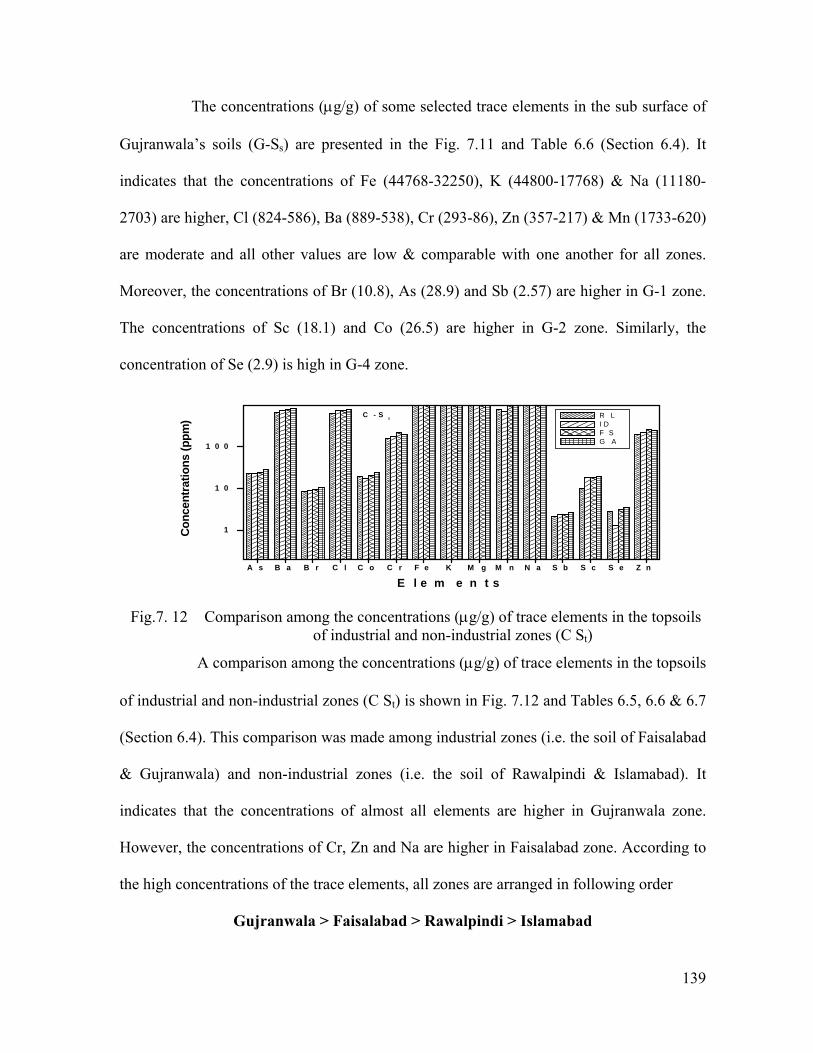
139
The concentrations (g/g) of some selected trace elements in the sub surface of
Gujranwala’s soils (G-Ss) are presented in the Fig. 7.11 and Table 6.6 (Section 6.4). It
indicates that the concentrations of Fe (44768-32250), K (44800-17768) & Na (11180-
2703) are higher, Cl (824-586), Ba (889-538), Cr (293-86), Zn (357-217) & Mn (1733-620)
are moderate and all other values are low & comparable with one another for all zones.
Moreover, the concentrations of Br (10.8), As (28.9) and Sb (2.57) are higher in G-1 zone.
The concentrations of Sc (18.1) and Co (26.5) are higher in G-2 zone. Similarly, the
concentration of Se (2.9) is high in G-4 zone.
A s B a B r C l C o C r F e K M g M n N a S b S c S e Z n
1
1 0
1 0 0
C - St
Co
nce
ntr
atio
ns
(pp
m)
E l e m e n t s
R L I D F S G A
Fig.7. 12 Comparison among the concentrations (g/g) of trace elements in the topsoils
of industrial and non-industrial zones (C St)
A comparison among the concentrations (g/g) of trace elements in the topsoils
of industrial and non-industrial zones (C St) is shown in Fig. 7.12 and Tables 6.5, 6.6 & 6.7
(Section 6.4). This comparison was made among industrial zones (i.e. the soil of Faisalabad
& Gujranwala) and non-industrial zones (i.e. the soil of Rawalpindi & Islamabad). It
indicates that the concentrations of almost all elements are higher in Gujranwala zone.
However, the concentrations of Cr, Zn and Na are higher in Faisalabad zone. According to
the high concentrations of the trace elements, all zones are arranged in following order
Gujranwala > Faisalabad > Rawalpindi > Islamabad

140
A s B a B r C l C o C r F e K M g M n N a S b S c S e Z n
1
1 0
1 0 0
C - Ss
Co
nce
ntr
atio
ns
(pp
m)
E l e m e n t s
I D F S R L G A
Fig.7. 13 Comparison among the concentrations (g/g) of trace elements in the sub soils
of industrial and non-industrial zones (CSs)
A comparison among the concentrations (g/g) of trace elements in the sub soils
of industrial and non-industrial zones (C Ss) is shown in Fig. 7.13 and Tables 6.5, 6.6 & 6.7
(Section 6.4). This comparison was made among industrial zones (i.e. the soil of Faisalabad
& Gujranwala) and non-industrial zones (i.e. the soil of Rawalpindi & Islamabad). It
indicates that the concentrations (g/g) of some selected trace elements such as Fe (44768-
27456), K (28916-19325), Mg (36827-33296) & Na (31306-2816) are higher, Cl (824-
692), Ba (889-762), Zn (226-179) & Mn (1733-605) are moderate and all other values are
low & comparable with one another for all zones. Moreover, the concentrations of all
elements are higher in Gujranwala zone. However, the concentrations of Sc (17.6) & Zn
(226) are higher in Faisalabad zone and the concentration of Se (2.63) is higher in
Rawalpindi zone. However, the concentrations of all elements are lower in Islamabad zone
as compared to Rawalpindi, Faisalabad and Gujranwala zones.

141
A s B a B r C l C o C r F e K M g M n N a S b S c S e Z n
1
1 0
1 0 0
C o m p a r e
Co
nce
ntr
atio
ns
(pp
m)
E l e m e n t s
N o r w a y I n d i a F a is a l a b a d G u j r a n w a la
Fig.7. 14 Comparison among the concentrations (g/g) of trace elements in the national
and international soils (Compare)
A comparison among the concentrations (g/g) of trace elements in the
national and international soils (Compare) is shown in Fig. 7.14 and Table 6.8 (Section
6.4). This comparison was made among national soils (i.e. Faisalabad & Gujranwala) and
international soils (i.e. Norway & India). All soils samples were analyzed through NAA
technique. The histogram indicates that the concentrations of all the elements except Cr,
Mg, Zn, Na and Mn are higher in the soil of Gujranwala. However, the concentrations of
Cr, Zn and Na are higher in the soil of Faisalabad. Similarly, the concentrations of Mg and
Mn are high in the soil of Norway. However, the concentrations of elements are least in the
soil of India. According to the high concentrations of the trace elements, generally all
industrial and non-industrial zones are arranged in the following sequence
Gujranwala > Faisalabad > Norway > India

142
A s B a B r C l C o C r F e K M g M n N a S b S c S e Z n
1
1 0
1 0 0
L e a c h
Co
nce
ntr
atio
ns
(pp
m)
E l e m e n t s
F S t F S s G S t G S s
Fig.7. 15 Leaching tendencies of some selected trace elements for Faisalabad and Gujranwala soils (Leach)
Leaching tendency of some selected trace elements was observed for Faisalabad
and Gujranwala soils, which is indicated in the Fig. 7.15 and Tables 6.5 & 6.6 (Section
6.4). The elements (Ba, Cr, As, Na, Cl, K, Br & Mg) due to high leaching tendency move
from topsoil to sub soil very easily as compared to other (Mn, Sb, Sc, Co, Se, Fe & Zn)
elements. This behavior was observed in the soils of both Faisalabad and Gujranwala. So
the quantities of the elements (Ba, Cr, As, Na, Cl, K, Br & Mg) are higher in sub soils (Ss)
as compared to the topsoil (St). This behavior is also conformed by the evidence of
observed high EC values (4.3 S/cm) at topsoil as compared to sub-soil (2.1S/cm) values.
7.5. Faisalabad and Gujranwala Crops
The four selected varieties of harvested crops namely wheat, rice, maize and
millet were collected within the vicinity of industrially polluted areas of Faisalabad and
Gujranwala. In this regard, 55 wheat samples, 37 rice samples, 45 maize samples and 41
millet samples were collected from twelve different sites in the fields as mentioned in the
samples location maps in section 4.1.1. Each species was then separated in to its fruits
(grains), leaves, stems and roots to evaluate their hazardous effects on animals and human

143
health. The results for elemental concentrations in the grains and leaves have been
presented in Tables 6.9a and 6.10 a respectively (section 6.5) for Faisalabad’s crops.
Similarly, the Tables 6.9 b and 6.10 b for grains and leaves respectively (section 6.5)
represent the results for Gujranwala’s crops. Moreover, the behavior of some important
selected elements is represented in Figures 7.16 to 7.33. According to the sample
identification scheme (section 4.1.4), Faisalabad industrial area was divided into four zones
(i.e. F-1, F-2, F-3 & F-4). F-1 represents the area of Industrial Estate, F-2 represents the
area of Ghulam Muhammad abad, F-3 represents the area of Peoples Colony and F-4
represents the area of Sitara Colony. Similarly, Gujranwala industrial area was divided into
four zones (i.e. G-1, G-2, G-3 & G-4). The areas of Dhula, Garjakh, Small Industrial Estate
and Muhammad Nagar are represented by G-1, G-2, G-3 & G-4 respectively.
7.5.1. Faisalabad and Gujranwala Wheat
All over the world, about 70% of human diet consists of cereals and legumes. The
yield capacity of wheat crop depended on some essential factors such as type of soil, wheat
variety, amount/ type of fertilizer, atmospheric conditions, pH, EC etc. of soil. In each
wheat sample, 26 trace elements have been determined quantitatively among which there
are 10 essential, 06 non-essential, 03 toxic and 07 rare earth elements. As mentioned in the
table 6.9a, the harvested wheat grains in F-3 zone contain Eu, Co, Fe, Cs & Sb elements in
the high concentrations. The elemental concentrations of Mg, Cl, Cr, Hf, Se, La, Na & Sm
are high in those samples, which were cultivated on F-1 zone. In the F-2 zone elemental
concentrations of Br, Al, As, Ce, Yb, Mn, Zr, Rb, Zn &. Sc is high and the elemental
concentrations of Ba, Ta, K & Th are high in the sown wheat grains from the F-4 zone.

144
A s B r C l C o S b S e T h
0 . 0 1
0 . 1
1
Co
nce
ntr
atio
ns
(pp
m)
E l e m e n t s
F - 1 F - 2 F - 3 F - 4
Fig.7.16. Level of toxic elements concentration for wheat grains grown in Faisalabad areas
The comparison results of Faisalabad wheat grains (fruits) for the elemental
concentrations revealed that the F-1 zone is the most contaminated among other zones as
shown in the Fig. 7.16, while the elemental concentrations are very low in F-4 zone.
Among all the elements, the chlorine concentration (4846-1348) is high in all zones. The
concentration values of each element are comparable with one another for all zones.
According to the high concentration of elements, the intensity of toxicity in the specified
zones of Faisalabad is decreased in the following pattern:
F-1 F-2 F-3 F-4
The results of randomly selected 04 zones for Faisalabad wheat leaves are shown
in Table 6.10.a (section 6.5). According to the table, the elemental concentrations of Ba,
As, Hf, Ce, Fe, Na, Yb, K, Se, La, Sc, Th & Zn are high in the leaves of wheat crop
cultivated in F-1 zone. The elemental concentrations of Mg, Cl, Sb, Cr, Sm & Zr are high
in F-3 zone. The elemental concentrations of Cs, Ta, Mn & Al are high in the F-2 zone
whereas the elemental concentrations of Br, Eu, Co & Rb are high in the F-4 zone.

145
A s B r C l C o S b S e T h
0 . 1
1
1 0
Co
nce
ntr
atio
ns
(pp
m)
E l e m e n t s
F - 3 F - 1 F - 2 F - 4
Fig. 7.17 Level of toxic elements concentration for wheat leaves grown in Faisalabad areas
The concentration levels of some selected important elements, which were present
in Faisalabad’s wheat leaves, are illustrated in the Fig. 7.17. It is indicated that the wheat
crop leaves grown in the F-1 zone are more contaminated than the leaves grown in other
zones of Faisalabad. Moreover, the elemental concentrations of Br (24.8-10.3) & Cl (6223-
2209) collected from all sites, are higher among other elements. In F-3 zone, the
concentrations of As (0.9) & Cl (2209) are low while the Se (0.18) & Sb (0.1) have low
concentrations in F-2 zone. In Faisalabad’s wheat crop, all elemental concentration values
for leaves are higher as compare to their grains.
Grown wheat crop was also collected from 06 different industrial places of
Gujranwala. In each sample, 29 trace elements including 09 essential, 06 non-essentials, 03
toxic and 06 rare earth elements have been explore. According to the table 6.9.b, the
elemental concentrations of Fe, Sm & Zr are high in the grains of wheat crop, which was
cultivated in G-3 zone. The elemental concentrations of Ce, As, K, Ba, Br, Mg, Eu, Zn, Hf,
Th, La, Yb, Sb, Ta & Na are high in G-1 zone. The elemental concentrations of Al & Se
are high in the G-4 zone whereas the elemental concentrations of Rb, Cl, Co, Mn, Cr, Cs,
Sc & V are high in the G-2 zone. The comparison results of wheat grains for the elemental
concentrations reveal that G-1 zone is the most polluted while G-4 is the least polluted.

146
A s B r C l C o S b S e T h
0 . 0 1
0 . 1
1
Co
nce
ntr
atio
ns
(pp
m)
E l e m e n t s
G - 1 G - 2 G - 3 G - 4
Fig. 7.18 Level of toxic elements concentration for wheat grains grown in Gujranwala areas
It is illustrated from the Fig. 7.18 that the concentration values of each element
are comparable with one another for all zones except for Sb (0.1-0.01) & Co (0.059-0.016),
which are very low. The concentration of Cl (327-195) is higher than all other elements in
all zones. Moreover, according to the high concentration values of concerned elements, the
intensity of the toxicity in the specified zones of Gujranwala was increased as follows
G-4 G-3 G-2 G-1
The results of randomly selected 04 zones for Gujranwala wheat leaves are shown
in Table 6.10.b (section 6.5). According to the table, the elemental concentrations of Ba,
La, Mg, Br, Eu, Hf, Sb, K & Se are higher in the leaves of wheat crop, which was
cultivated in G-3 zone. The elemental concentrations of Yb, As, Zr, Na & Mn are higher in
G-1 zone. The elemental concentrations of Sm, Al, Sc & Rb are higher in the zone of G-4
whereas the elemental concentrations of Th, Ce, Fe, Cl, Co, Ta, Cr, Zn & Cs are higher in
the G-2 zone.

147
A s B r C l C o S b S e T h
0 . 0 1
0 . 1
1
1 0
Co
nce
ntr
atio
ns
(pp
m)
E l e m e n t s
G - 3 G - 1 G - 4 G - 2
Fig. 7.19 Level of toxic elements concentration for wheat leaves grown in Gujranwala area
The concentration levels of some selected important elements, which were present
in Gujranwala’s wheat leaves, are illustrated in the Fig. 7.19. It indicates that the elemental
concentrations of Br (11.9-4.5) & Cl (325-135) collected from all zones are higher among
other elements. The concentrations of Br (11.9) & Se (0.61) are high in G-3 zone.
Similarly, the concentrations of Br (4.5) & Sb (0.03) are low in G-1 zone. According to the
concentration values, the elements are arranged in the following order for all zones
Cl > Br > As > Co > Se > Th > Sb
A s B r C l C o S b S e S r T h
0 . 1
1
W h e a t - c r o p
Co
nce
ntr
atio
ns
(g
/g)
E l e m e n t s
F r u i t s L e a v e s S t e m s R o o t s
Fig. 7.20 Bio-distribution pattern for wheat crop

148
The pattern of bio-distribution for wheat crop into its parts such as fruits (grains),
leaves, stems & roots are illustrated below and in the Histogram 7.20. The concentration of
Cl is higher in all parts of the wheat species. The elemental concentrations of Se, As & Sb
are comparable with one another. The concentrations of Co, Th & Br are higher in all parts.
In short, the activity increases in the following sequence and indicates that the roots are the
most polluted (in term of high concentration of elements) with industrial effluents as
compared to other parts of the plants and the fruits (grains) have least concentration of all
concerned elements.
Fruits (Grains) Leaves Stems Roots
7.5.2. Faisalabad and Gujranwala Rice
Grown crop of rice was collected from more than 12 areas of Faisalabad and
Gujranwala. In each sample of Faisalabad & Gujranwala rice crop, total 26 elements were
determined, among which there were 08 essential, 06 non-essential, 03 toxic and 06 rare
earth elements. The concentrations of all elements are expressed in μg/g unit.
Cultivated rice crop was collected from more than 04 zones of Faisalabad. The
results of rice fruit (grains) obtained from 02 selected zones i.e. F-3 and F-2 are presented
in Table 6.9.a (Section 6.5). According to the table, in the fruits (grains) of Faisalabad rice,
the concentrations of elements such as Cr, Ba, Br, Yb, Rb, Se, Zn & Zr are high in the zone
of F-3. While the elemental concentration of Cl, As, Ce, Eu, Co, Hf, Cs, Lu, Fe, K, La, Sb,
Mn, Ta, Na, Sc & Th are higher in the rice (grains) harvested in the F-2 zone.

149
A s B r C l C o S b S e T h
0 . 0 1
0 . 1
1
1 0
Co
nce
ntr
atio
ns
(pp
m)
E l e m e n t s
F - 3 F - 2
Fig. 7.21 Level of toxic elements concentration for rice grains grown in Faisalabad areas
The Fig. 7.21 indicates that the concentrations of Cl (1300-1130) & Br (9.8-8.0)
are higher among all other selected elements in all zones where the rice crop was cultivated
in Faisalabad. While the concentrations of Th (0.36-0.2), Sb (0.47-0.1), Co (0.14-0.23), Se
(0.3-0.38) and As (0.4-0.3) are low in quantity for all zones. The concentration values for
all elements are higher in zone F-2 as compared to zone F-3. Therefore, due to high
concentration of elements, the toxic level of F-2 zone is higher than F-3 zone as shown in
the following descending order
F-2 > F-3
The results of randomly selected 2 zones for Faisalabad rice leaves have been
shown in Table 6.10.a (Section 6.5), which indicates that the concentrations of Mn, Br, K,
Cr, Eu, Sb, Hf, Rb, Sc, Yb, Se & Zr elements are high in the rice leaves grown in the zone
of F-3. While the elemental concentrations of As, Cl, Ba, Ce, Fe, Co, Lu, Cs, La, Th, Na,
Ta & Zn are higher in the zone of F-2.

150
A s B r C l C o S b S e T h
0 . 0 1
0 . 1
1
1 0
Co
nce
ntr
atio
ns
(pp
m)
E l e m e n t s
F - 3 F - 2
Fig. 7.22 Level of toxic elements concentration for rice leaves grown in Faisalabad areas
The Fig. 7.22 indicates that the concentrations of As (2.7), Co (0.81) & Cl (5723)
are higher in F-2 zone as compare to F-3 zone for rice leaves. The Br (5.8) & Se (0.23)
concentrations are low in F-2 zone. The concentrations of Th (0.2-0.21) and Sb (0.4-0.36)
are comparable to each other in all zones.
Gujranwala rice fruit (grains) was collected from 04 different zones. The results
of randomly selected 03 zones i.e. G-1, G-2 and G-3 were shown in Table 6.9b (Section
6.5). According to the table, the elemental concentrations of As, Br, Fe, Hf & Yb are higher
in the grains of rice crop which was cultivated in G-3 zone. The elemental concentrations
of Ba, Ce, Co, Cr, Eu, Lu, Rb, Sc, Ta & Zn are higher in G-1 Zone whereas the elemental
concentrations of Cl, Cs, K, La, Mn, Na, Sb, Sc, Th & Zr are higher in the G-2 zone.
A s B r C l C o S b S e T h
0 . 1
1
Co
nce
ntr
atin
(p
pm
)
E l e m e n t s
G - 1 G - 3 G - 2
Fig. 7.23 Level of toxic elements concentration for rice grains grown in Gujranwala areas
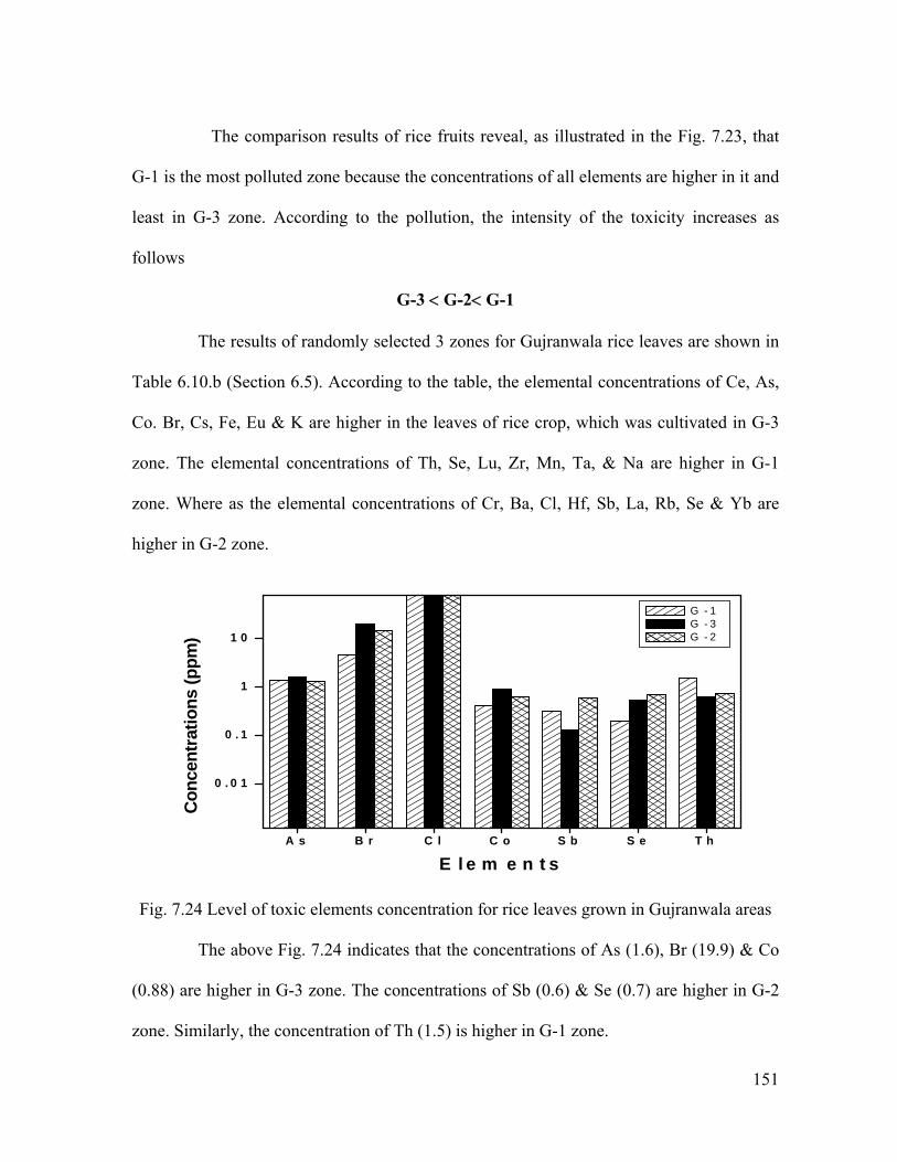
151
The comparison results of rice fruits reveal, as illustrated in the Fig. 7.23, that
G-1 is the most polluted zone because the concentrations of all elements are higher in it and
least in G-3 zone. According to the pollution, the intensity of the toxicity increases as
follows
G-3 G-2 G-1
The results of randomly selected 3 zones for Gujranwala rice leaves are shown in
Table 6.10.b (Section 6.5). According to the table, the elemental concentrations of Ce, As,
Co. Br, Cs, Fe, Eu & K are higher in the leaves of rice crop, which was cultivated in G-3
zone. The elemental concentrations of Th, Se, Lu, Zr, Mn, Ta, & Na are higher in G-1
zone. Where as the elemental concentrations of Cr, Ba, Cl, Hf, Sb, La, Rb, Se & Yb are
higher in G-2 zone.
A s B r C l C o S b S e T h
0 . 0 1
0 . 1
1
1 0
Co
nce
ntr
atio
ns
(pp
m)
E l e m e n t s
G - 1 G - 3 G - 2
Fig. 7.24 Level of toxic elements concentration for rice leaves grown in Gujranwala areas
The above Fig. 7.24 indicates that the concentrations of As (1.6), Br (19.9) & Co
(0.88) are higher in G-3 zone. The concentrations of Sb (0.6) & Se (0.7) are higher in G-2
zone. Similarly, the concentration of Th (1.5) is higher in G-1 zone.

152
7.5.3. Faisalabad and Gujranwala Maize
Harvested crop of maize was obtained from more than 06 areas of Faisalabad and
Gujranwala. In each sample of Faisalabad maize crop total 26 elements were determined,
among which there are 08 essential elements, 06 non-essential elements, 03 toxic elements
and 06 rare earth elements. Similarly, in each sample of Gujranwala maize crop total 24
elements were determined, among which there are 09 essential elements, 05 non-essential
elements, 02 toxic elements and 05 rare earth elements.
Grown maize crop was collected from more than 03 industrial areas of
Faisalabad. The result of maize fruit (grains), collected from 02 selected zones i.e. F-1 and
F-3, has been presented in Table 6.9.a (Section 6.5). According to the table, the
concentrations of Cl, Ba, Hf, Cs, Mn, Eu, Yb, Sc & K elements, for the cultivated crops of
Maize (Grains), are higher in the F-3 zone. Similarly the concentrations of Ce, As, Cr, Br,
Co, Na, Se, Fe, Sb, Sm, Ta, Sr, Tb, Zn, Th & Zr elements, for the cultivated crops of Maize
(Grains), are higher in the F-1 zone.
A s B r C l C o S b S e T h
0 . 0 1
0 . 1
1
1 0
Co
nce
ntr
atio
ns
(pp
m)
E l e m e n t s
F - 3 F - 1
Fig. 7.25 Level of toxic elements concentration for maize grains grown in Faisalabad areas
The comparison results of Faisalabad maize grains (fruits) for the elemental
concentrations revealed that the F-1 zone is the most contaminated among other zones as
shown in the Fig. 7.25, while the elemental concentrations are very low in F-3 zone.

153
Among all the elements, the chlorine concentration (800-700) is high in all the zones. The
concentration values of Br (3.86-4.12) and As (4.12-3.86) are moderate for all zones. While
the concentrations of Th (0.02-0.04), Sb (0.01-0.02), Co (0.01-0.03) and Se (0.16-0.2) are
low in quantity for all zones. The concentration values for all elements are higher in zone
F-1 as compared to zone F-3. Therefore, due to high concentration of elements, the toxic
level of F-1 zone is higher than F-3 zone as shown in the following descending order
F-1 > F-3
The results of randomly selected 02 zones for Faisalabad maize leaves are shown
in Table 6.10.a (Section 6.5). According to table, the concentrations of elements Co, Ba,
Cl, Hf, Cr, Mn, Cs, Rb, Eu, Na, Yb, Ta, & Sm, for the cultivated crops of maize (Leaves),
are higher in the F-3 zone. Similarly the concentrations of Br, As, Ce, K, Sb, Th, Sc, Fe, Zr,
Sr, Tb, Zn & Se elements, for the cultivated crops of maize (Leaves), are higher in the F-1
zone.
A s B r C l C o S b S e T h
0 . 0 1
0 . 1
1
Co
nce
ntr
atio
ns
(pp
m)
E l e m e n t s
F - 3 F - 1
Fig. 7.26 Level of toxic elements concentration for maize leaves grown in Faisalabad areas
The concentration levels of some selected important elements, which were present
in Faisalabad’s maize leaves, are illustrated in the Fig. 7.26. It is indicated that the maize
crop leaves grown in the F-1 zone has higher elemental concentrations than the leaves
grown in other zones of Faisalabad. Moreover, the elemental concentration of Cl (919-818)

154
collected from all sites, is higher among other elements. The concentration values of Br
(4.0-4.76) are moderate for all zones. The concentrations of As (0.72-0.82) & Se (0.2-0.32)
are comparable for both zones. The concentration values of Sb (0.03-0.06) & Co (0.09-
0.06) are very low in all zones. All the leaves values are higher than the values of all
elements present in the grains of Faisalabad maize crop.
Grown maize crop was collected from more than 03 industrial areas of
Gujranwala. The result of maize fruit (grains), collected from 02 selected zones i.e. G-2
and G-1, has been presented in Table 6.9b (Section 6.5). According to the table, the
concentrations of elements Yb, Br, Tb, Na, Sc, Ta & Cl, for the cultivated crops of Maize
(Grains), are highest in the G-2 zone. Similarly the concentrations of Th, Ca, Zn, Ce, Zr,
Co, Rb, Cs, Sb, Eu, Fe, Sc, Hf, K, Mn, Sr, & Cr elements, for the cultivated crops of Maize
(Grains), are higher in the G-1 zone.
A s B r C l C o S b S e T h
0 . 0 1
0 . 1
1
Co
nce
ntr
atio
ns
(pp
m)
E l e m e n t s
G - 2 G - 1
Fig. 7.27 Level of toxic elements concentration for maize grains grown in Gujranwala areas
It is illustrated from the Fig. 7.27 for the maize grains of Gujranwala that the
concentration values of As (0.3-0.4) & Se (0.12-0.21) are comparable with each other for
all zones. The concentration value of Cl (890-420) is higher than all other elements in all
zones. The concentrations of Br (2.38), As (0.3), Co (0.03), Sb (0.013), Th (0.011) & Se

155
(0.12) are low for G-2 zone while the concentration value of Cl (420) is low for G-1 zone.
Moreover, G-1 is the most polluted zone because the concentrations of all elements are
higher in it and least in G-2 zone. According to the high concentration values of concerned
elements, the intensity of the toxicity in the specified zones of Gujranwala maize grains is
increased as follows
G-2 G-1
The results of randomly selected 04 zones for Gujranwala maize leaves are shown
in Table 6.10.b (section 6.5). According to the table, the concentrations of elements Br, Yb,
Cl, Hf, K, Th, Rb, Ta, Na, Zr, Se, Tb & Mn, for the cultivated crops of Maize (Leaves), are
higher in the G-2 zone. Similarly the concentrations of elements Ca, Ce, Sb, Zn, Co, Sr, Cr,
Rb, Cs, Eu, Sc & Fe for the cultivated crops of Maize (Leaves), are higher in the G-1 zone.
A s B r C l C o S b S e T h
0 . 0 1
0 . 1
1
Co
nce
ntr
atio
ns
(pp
m)
E l e m e n t s
G - 2 G - 1
Fig. 7.28 Level of toxic elements concentration for maize leaves grown in Gujranwala area
The concentration levels of some selected important elements, which were present
in Gujranwala’s maize leaves, are illustrated in the Fig. 7.28. It indicates that the elemental
concentration of Cl (982-711) collected from all zones is higher among other elements. The

156
concentration of Br (4.83-1.52) is moderate. The concentrations of Co (0.04-0.08), Th
(0.02-0.04), As (0.04-0.05) & Sb (0.022-0.064) are comparable with one another. The
concentrations of Co (0.04), As (0.04), Sb (0.022) & Th (0.02) are low in G-2 zone.
Similarly, the concentrations of Br (1.52), Se (0.16) & Cl (711) are low in G-1 zone.
According to the concentration vales, the elements are arranged in the following order for
all zones
Cl > Br > Se > Co > As > Sb > Th
7.5.4. Faisalabad and Gujranwala Millet
Cultivated crop of millet was collected from more than 05 areas of Faisalabad and
Gujranwala. In each sample of Faisalabad’s millet crop, total 26 elements were determined,
among which there were 09 essential, 05 non-essential, 03 toxic and 06 rare earth elements.
Similarly, in each sample of Gujranwala’s millet crop total 31 elements were determined,
among which there were 10 essential, 05 non-essential, 03 toxic and 07 rare earth elements.
Harvested millet crop was collected from more than 02 industrial areas of
Faisalabad. The result of millet fruit (grains), collected from 02 selected zones i.e. F-3 and
F-2, has been presented in Table 6.9.a (Section 6.5). According to the table, the
concentrations of elements Cr, As, Eu, Sr, Br, Mn, Cs, Yb, Sb, Fe, Tb, K, Ta, La, Rb, Sc,
Th, & Na, for the cultivated crops of Millet (Grains), are higher in the F-2 zone. Similarly
the concentrations of elements Ca, Zr, Ce, Zn, Co, Se, Cl & Hf, for the cultivated crops of
Millet (grains), are higher in the F-3 zone.

157
A s B r C l C o S b S e T h
0 . 0 1
0 . 1
1
Co
nce
ntr
atio
ns
(pp
m)
E l e m e n t s
F - 2 F - 3
Fig. 7.29 Level of toxic elements concentration for millet grains grown in Faisalabad areas
The concentration levels of some selected important elements, which were present
in Faisalabad’s millet grains (fruits), are illustrated in the Fig. 7.29. It is indicated that
among all the elements, the chlorine concentration (470-710) is high in all zones. The
concentration values of Br (1.2-0.94) and As (2.79-0.2) are moderate for all zones. While
the concentrations of Th (0.08-0.04), Sb (0.01-0.04), Co (0.06-0.04) & Se (0.01-0.03) are
low in quantity and are comparable with one another for all zones. The concentration values
for all elements are higher in zone F-1 as compared to zone F-3. Therefore, due to high
concentration of elements, the toxic level of F-1 zone is higher than F-3 zone as shown in
the following descending order
F-1 > F-3
Harvested millet crop leaves were collected from more than 02 industrial areas
of Faisalabad. The result of millet leaves, collected from 02 selected zones i.e. F-3 and F-2,
has been presented in Table 6.10.a (Section 6.5). According to the table, the concentrations
of elements As, Yb, Br, Ca, Ta, Ce, K, Cr, Fe, Hf, Tb, La, Rb, Sb, Mn, Se, Th & Co, for the
cultivated crops of Millet (Leaves), are higher in the F-2 zone. Similarly the concentrations
of elements Zr, Cs, Eu, Na, Sc, Zn, Sr & Cl, for the cultivated crops of Millet (Leaves), are
higher in the F-3 zone.

158
A s B r C l C o S b S e T h
0 . 0 1
0 . 1
1
1 0
Co
nce
ntr
atio
ns
(pp
m)
E l e m e n t s
F - 2 F - 3
Fig. 7.30 Level of toxic elements concentration for millet leaves grown in Faisalabad areas
The concentration levels of some selected important elements, which were present
in Faisalabad’s millet leaves, are illustrated in the Fig. 7.30. It is indicated that the millet
crop leaves grown in the F-1 zone have higher elemental concentrations than the leaves
grown in other zones of Faisalabad. Moreover, the elemental concentration of Cl (4984-
6098) collected from all sites, is higher among other elements. The concentration values of
Br (23.5-13.7) are moderate for all zones. The concentrations of As (0.58-0.52), Se (0.1-
0.09), Sb (0.09-0.05) & Co (0.18-0.15) are very low and are comparable with one another.
Harvested millet crop was collected from more than 03 industrial areas of
Gujranwala. The results of millet fruit (grains), collected from 03 selected zones i.e. G-1,
G-2 and G-3, have been presented in Table 6.9.b (Section 6.5). According to the table, the
concentrations of elements Co, Br, Ce, Eu, Na, Hf & Ta, for the cultivated crops of Millet
(Grains), are higher in the G-1 zone. Similarly the concentrations of elements Cs, Zr, Lu,
Th, Sc, Tb & Rb, for the cultivated crops of Millet (Grains), are higher in the G-3 zone.
Also the concentrations of elements Cl, Al, Zn, As, Ca, K, Cu, Fe, Mg, La, Sb, Mn, Se, Yb,
Ti & Cr, for the cultivated crops of Millet (Grains), are higher in the G-2 zone.

159
A s B r C l C o S b S e T h
1 E - 3
0 . 0 1
0 . 1
1
1 0
Co
nce
ntr
atio
n (
pp
m)
E l e m e n t s
G - 1 G - 3 G - 2
Fig. 7.31 Level of toxic elements concentration for millet grains grown in Gujranwala areas
It is illustrated from the Fig. 7.31 for the millet grains harvested in Gujranwala
that the concentration values of all elements are high in G-1 zone, moderate in G-2 zone
and low in G-3 zone. However, the concentration value of Cl (830-390) is high, Br (96-62)
is moderate and As (0.4-0.1), Co (0.08-0.05), Sb (0.04-0.02), Th (0.04-0.024) & Se (0.07-
0.05) are low and comparable with one another for all zones. According to the high
concentration values of concerned elements, the intensity of the toxicity in the specified
zones of Gujranwala maize grains is increased as follows
G-3 G-2 G-1
Harvested millet crop was collected from more than 03 industrial areas of
Gujranwala. The result of millet leaves, collected from 03 selected zones i.e. G-1, G-2 and
G-3, has been presented in Table 6.10.b (Section 6.5). According to the table, the
concentrations of elements Ti, Al, Br, As, Ca, Fe, Co, Mn, Hf, Mg, Sb, K, Sc, Na, Th &
Ce, for the cultivated crops of Millet (Leaves), are higher in the G-1 zone. Similarly the
concentrations of elements, Cs, Zr, Rb, Se, Yb, Tb, Zn, La & Eu, for the cultivated crops of
Millet (Leaves), are higher in the G-3 zone. Also the concentrations of elements Cl, Ta, Lu
& Cr, for the cultivated crops of Millet (Leaves), are higher in the G-2 zone.

160
A s B r C l C o S b S e T h
0 . 0 1
0 . 1
1
1 0
Co
nce
ntr
atio
ns
(pp
m)
E l e m e n t s
G - 1 G - 2 G - 3
Fig. 7.32 Level of toxic elements concentration for millet leaves grown in Gujranwala areas
The concentration levels of some selected important elements, which were present
in Gujranwala’s millet leaves, are illustrated in the Fig. 7.32. It indicates that the elemental
concentration of Cl (6352-2706), collected from all zones. is higher among other elements.
The concentration value of Br (27-4.0) is moderate. The concentrations of Co (1.8-0.1) &
As (1.3-0.26) are low and Sb (0.19-0.06), Th (0.4-0.07) & Se (0.21-0.15) are comparable
with one another, for all zones. The concentrations of Co (0.1), Sb (0.06), Th (0.07) & Se
(0.15) are low in G-2 zone. Similarly, the concentrations of Br (4.0), As (0.26) & Cl (2706)
are low in G-3 zone. According to the concentration values, the elements are arranged in
the following order for all zones
Cl > Br > As > Co > Th > Se > Sb
7.5.5 Comparison among the cereal grains for the evaluation of toxic levels
To evaluate the toxic levels among the cereal grains, which had been grown
within the vicinity of industrial zones of Faisalabad and Gujranwala, a comparison is
presented in Fig. 7.33a & b.

161
A s C d C o C r C u F e M n N i P b S b S e
0 . 0 1
0 . 1
1 0
F - C r o p s
Co
nce
ntr
atio
ns
(pp
m)
E l e m e n t s
W h e a t R i c e M a i z e M i l l e t
Fig. 7.33.a Comparison among the grains of wheat, rice, maize and millet cereals from
Faisalabad areas for the evaluation of toxic levels
A s C d C o C r C u F e M n N i P b S b S e
0 . 0 1
0 . 1
1
1 0
G - C r o p s
Co
nce
ntr
atio
ns
(pp
m)
E l e m e n t s
W h e a t R i c e M a i z e M i l l e t
Fig. 7.33.b Comparison among the grains of wheat, rice, maize and millet cereals from Gujranwala areas for the evaluation of toxic levels
In this comparison, eleven heavy and toxic metals such as As, Cd, Co, Cr, Cu, Fe,
Mn, Ni, Pb, Sb and Se were selected. These metals were present in all selected cereals such
as wheat, rice, maize and millet, which were cultivated in Faisalabad and Gujranwala areas.
Their concentrations were higher as compared to the recommended values, which was due
to the contribution of industrial effluents. It was observed that the crop species are selective

162
for selected metals. For example the concentrations of Cr & Cu were high in millet crop,
which was collected from both Faisalabad and Gujranwala areas. The concentrations of Cd
& Pb were high in maize crop, which was collected from both Faisalabad and Gujranwala
areas. Similarly, wheat and rice crops were enriched in Fe and Sb respectively. Moreover,
it reveals that the toxic elemental concentrations are higher in millet and lower in wheat.
The toxic activity decreases in the following sequence, which indicates that wheat crop is
the least affected by the industrial effluents as compared to the other cereal crops.
Millet Maize Rice Wheat
7.6. Faisalabad and Gujranwala Vegetables
Vegetables are staple part of food and are widely consumed in all over the world.
The determination of metal contents in vegetables is important from the viewpoint of crop
yield technology, food nutrition and health impacts. The differences for the accumulation
of mineral/ metal contents in the edible portions of vegetables are depending upon the soil
composition and the rate of uptake of minerals/ metals by each plant. A variety of common
vegetables had been collected, in summer and winter seasons, for present work, from
selected zones of Faisalabad and Gujranwala. Out of 13 vegetables there are 06 summer
vegetables (i.e. brinjal, baffle gourd, Ridged gourd, tomato, pumpkin and bitter gourd), 03
winter vegetables (i.e. cabbage, mustard and spinach) and 04 under ground vegetables (i.e.
potato, turnip, radish and carrot). Their elemental concentrations (µg/g) results for
Faisalabad’s vegetables have been presented in Tables 6.11.a and 6.12.a, mentioned in
section 6.6. Moreover, the elemental concentrations (µg/g) results for Gujranwala’s
vegetables have been presented in Tables 6.11.b and 6.12.b, mentioned in the section 6.6.

163
7.6.1. Faisalabad and Gujranwala Summer Vegetables
Grown summer vegetables 1 & 2 were collected from more than 04 areas of
Faisalabad and Gujranwala. In the sample of Faisalabad summer vegetables-1 (Baffle
gourd, Ridged gourd & Pumpkin), total 28 elements were determined, among which there
are 08 essential elements, 06 non-essential elements, 03 toxic elements and 06 rare earth
elements. While in the sample of Faisalabad summer vegetables-2 (Brinjal, Tomato &
Bitter gourd), total 29 elements were determined, among which there are 10 essential
elements, 06 non-essential elements, 03 toxic elements and 06 rare earth elements.
Similarly, in the sample of Gujranwala summer vegetables-1 (Baffle gourd, Ridged gourd
& Pumpkin), total 27 elements were determined, among which there are 08 essential
elements, 06 non-essential elements, 03 toxic elements and 07 rare earth elements. While in
the samples of Gujranwala summer vegetables-2 (Brinjal, Tomato & Bitter gourd), total 28
elements were determined, among which there are 09 essential elements, 06 non-essential
elements, 03 toxic elements and 07 rare earth elements.
The result of the edible parts of the cultivated summer vegetables-1 (Baffle
gourd, Ridged gourd & Pumpkin), which were grown on the industrial zones of Faisalabad,
has been presented in Table 6.11.a (Section 6.6). According to the table, for the cultivated
Faisalabad summer vegetables-1, the concentrations of elements Br, Rb, Se, Na, Ta & Ti,
are higher in the edible portion of Baffle gourd. Similarly the concentrations of elements
Yb, Cs, As, Hf, Co, Lu, Zn Fe, La, Zr Mn, Sb, V & Sc for the edible portion of Ridged
gourd, are higher. Moreover, the concentrations of elements Cl, Ba, Ce, Eu, Cr, K & Th,
for the edible portion of Pumpkin, are high.

164
A s B r C l C o S b S e T h
0 . 0 1
0 . 1
1
1 0
Co
nce
ntr
atio
ns
(pp
m)
E l e m e n t s
B u f f l e g o u r d R i d y g o u r d P u m p k i n
Fig. 7.34 Toxicity level in the summer vegetables-1 (edible portion) grown in Faisalabad areas
The concentration levels of some selected important elements, which were present
in Faisalabad’s summer vegetables-1 (edible portion), are illustrated in the Fig. 7.34. It is
indicated that the chlorine concentration (4600-1460) is high and bromine concentration
(1.86-17.8) is moderate while the values of all other elements are low and comparable with
one another in all vegetables. The values of Br (17.8) & Se (0.21) are higher for Baffle
gourd. While the concentrations of As (0.72), Sb (0.06) & Co (0.43) are higher for Ridged
gourd. Similarly, the concentration values for Cl (4600) & Th (0.06) are higher for
Pumpkin. In short, due to high concentration of elements, the vegetables are shown in the
following descending order
Ridged gourd > Baffle gourd > Pumpkin
The result of the edible portions of the cultivated summer vegetables-2 (Brinjal,
Tomato & Bitter gourd), which were grown on the industrial area of Faisalabad, has been
presented in Table 6.11.a (Section 6.6). According to the table, for the cultivated
Faisalabad summer vegetables-2, the concentrations of elements Th, Cr, Zr, Fe, Se, Ba &
Hf are higher in the edible portion of Brinjal. Similarly the concentrations of elements As,
Lu, Br, K, Co, Sm, Cu & Ca, in the edible portion of Tomato, are higher. Moreover, the
concentrations of elements Ce, Sc, Cl, Zn, Cs, Eu, Yb, La, Sb, Mn, Rb, Ta & Na, in the
edible portion of Bitter gourd, are high.

165
A s C d C o C r C u F e M n N i P b S b S e
0 . 1
1
F - S u m m e r V e g e t a b l e s
Co
nce
ntr
atio
ns
(pp
m)
E l e m e n t s
B r i n j a l T o m a t o B i t t e r g o u r d
Fig. 7.35 Toxicity level in the summer vegetables-2 (edible portion) grown in Faisalabad areas
The concentration levels of some selected important elements, which were present
in Faisalabad’s summer vegetables-2 (edible portion), are illustrated in the Fig. 7.35. It is
indicated that the chlorine concentration (1810-1300) is high and bromine concentration
(65-6.3) is moderate while the values of all other elements are low and comparable with one
another in all vegetables. The values of Br (65), As (0.53) & Co (0.4) are higher for Tomato.
The concentrations of Sb (0.06) and Cl (1810) are higher for Bitter gourd. The concentration
values for Se (0.24) and Th (0.11) are higher for Brinjal. In short, due to high concentration
of elements, the vegetables are shown in the following descending order
Tomato > Bitter gourd > Brinjal
The result of the edible parts of the cultivated summer vegetables-1, which were
grown on the industrial area of Gujranwala, has been presented in Table 6.12.a (Section
6.6). According to the table, for the cultivated Gujranwala summer vegetables-1, the
concentrations of elements As, Yb, Co, Eu, Hf, Mn, Fe, Sm & Cs are higher in the edible
portions of Ridged gourd. Similarly the concentrations of elements Ba, Ce, Br, Cl, La, Cr,
Zr, Lu, Rb, Zn, Th & K, in the edible portions of Pumpkin, are higher. Moreover, the
concentrations of elements Sb, Ta, Sc & Se, in the edible portions of Baffle gourd, are high.

166
A s B r C l C o S b S e T h
0 . 0 1
0 . 1
1
Co
nce
ntr
atio
ns
(pp
m)
E l e m e n t s
R i d y g o u r d P u m p k i n B u f f l e g o u r d
Fig. 7.36 Toxicity level in the summer vegetables-1 (edible portion) grown in Gujranwala areas
The concentration levels of some selected important elements, which were present
in Gujranwala’s summer vegetables-1 (edible portion), are illustrated in the Fig. 7.36. It is
indicated that the chlorine concentration (4377-1267) is high and bromine concentration
(1.64-1.49) is moderate while the values of all other elements are low and comparable with
one another in all vegetables. The values of Sb (0.07) & Se (0.35) are higher for Baffle
gourd, while the concentrations of As (0.64) & Co (0.27) are higher for Ridged gourd.
Similarly, the concentration values for Br (1.64), Cl (4377) & Th (0.047) are higher for
Pumpkin. In short, due to high concentration of elements, the vegetables are shown in the
following descending order
Ridged gourd > Baffle gourd > Pumpkin
The result of the edible portions of the cultivated summer vegetables-2 (Brinjal,
Tomato & Bitter gourd), which were grown on the industrial area of Gujranwala, has been
presented in Table 6.12.a (Section 6.6). According to the table, the concentrations of
elements Zr, Ba, Cr, Yb, Cs, Eu, La, Mn, Rb, Na, Sb & Cl are high in the Bitter gourd and
the concentrations of elements As, Th, Ca, K & Zn, in the Tomato, are high. The elemental
concentrations of Br, Ce, Fe, Lu, Sc, Ta, Se, Hf, Sm & Co, in the Brinjal, are high.

167
A s C d C o C r C u F e M n N i P b S b S e
0 . 1
1
G - S u m m e r V e g e t a b l e s
Co
nce
ntr
atio
ns
(pp
m)
E l e m e n t s
B i t t e r g o u r d T o m a t o B r i n j a l
Fig. 7.37 Toxicity level in the summer vegetables-2 (edible portion) grown in Gujranwala areas
The concentration levels of some selected important elements, which were present
in Gujranwala’s summer vegetables-2 (edible portion), are illustrated in the Fig. 7.37. It is
indicated that the chlorine concentration (725-547) is high and bromine concentration (52-
9.4) is moderate while the values of all other elements are low and comparable with one
another in all vegetables. The values of Br (52), As (0.44) & Th (0.23) are higher for
Tomato. The concentrations of Co (0.35) and Se (0.29) are higher for Brinjal. Similarly, the
concentration values for Sb (0.5) and Cl (725) are higher for Bitter gourd. In short, due to
high concentration of elements, the vegetables are shown in the following descending order
Brinjal > Bitter gourd > Tomato
7.6.2. Faisalabad and Gujranwala Winter Vegetables
Grown winter vegetables (whose edible parts are leaves) were collected from
more than 04 areas of Faisalabad and Gujranwala. In each sample of Faisalabad &
Gujranwala winter vegetables, total 30 elements were determined, among which there were
10 essential, 06 non-essential, 03 toxic and 07 rare earth elements. The result of the edible
portion (leaves) of the cultivated winter vegetables (Mustard, Cabbage & Spinach), which
were grown on the industrial area of Faisalabad, has been presented in Table 6.11.b

168
(Section 6.6). According to the table, the concentrations of elements Ba, Cr, Zr, Cs, Eu,
Sm, Cu, Yb, Hf, La, Sb, Mn, Sc, Th & Co are higher in the edible portion (leaves) of
Mustard. Similarly, the concentrations of elements Ti, Ce, Se, Fe, Ta & As, for the edible
portion (leaves) of Cabbage, are higher. Moreover, the concentrations of elements Br, Lu,
K, Zn, Na, Rb, Mg & Cl, for the edible portion (leaves) of Spinach, are high.
A s C d C o C r C u F e M n N i P b S b S e
0 . 0 1
0 . 1
1
F - W i n t e r V e g e t a b l e s
Co
nce
ntr
atio
ns
(pp
m)
E l e m e n t s
M u s t a r d C a b b a g e S p i n a c h
Fig. 7.38 Level of toxic elements concentration for winter vegetable leaves grown in
Faisalabad
The concentration levels of some selected important elements, which were
present in Faisalabad’s winter vegetable leaves, are illustrated in the Fig. 7.38. It indicates
that the concentration of Cl (6321-1438) is high and the concentration of Br (32-4.7) is
moderate for all vegetables. The concentrations of As (2.73) and Se (0.59) are high in
cabbage leaves. The concentrations of Sb (0.1), Co (0.68) and Th (0.33) are high in
mustard leaves and the concentrations of Br (32) and Cl (6321) are high in spinach leaves.
The result of the edible portion (leaves) of the cultivated winter vegetables, which
were grown on the industrial area of Gujranwala, was presented in Table 6.12.b (Section
6.6). According to the table the concentrations of elements As, Zn, Ba, Ce, Fe, Hf, Mn, Sc,
Co, Sm, Cu, Ta, Cs, Ti, Yb, Cl & Br are higher in the leaves of Mustard. Similarly the

169
concentrations of elements Lu & Se, for the leaves of Cabbage, are higher. Moreover, the
concentrations of elements Cr, Al, Eu, Th, K, La, Zr, Sb & Rb, for the leaves of Spinach,
are high.
A s C d C o C r C u F e M n N i P b S b S e
0 . 1
1
G - W i n t e r V e g e t a b l e s
Co
nce
ntr
atio
ns
(pp
m)
E l e m e n t s
M u s t a r d C a b b a g e S p i n a c h
Fig. 7.39 Level of toxic elements concentration for winter vegetable leaves
(edible portion) grown in Gujranwala
The concentration levels of some selected important elements, which were
present in Gujranwala’s winter vegetable leaves, are illustrated in the Fig. 7.39. It indicates
that the concentrations of Br (35), As (2.1), Co (0.49) and Cl (7252) are high in mustard
leaves. The concentration of Se (0.6) is high in cabbage leaves. Similarly, the
concentrations of Th (0.37) and Sb (0.4) are high in spinach leaves. The concentration of Cl
(7252-1267) is high and the concentration of Br (35-30.6) is moderate for all vegetables.
7.6.3. Faisalabad and Gujranwala Under-ground Vegetables
Grown under ground vegetables, whose edible portions are roots were collected
from more than 04 areas of Faisalabad and Gujranwala. In each sample of Faisalabad and
Gujranwala under ground vegetables, total 27 elements were determined, among which
there were 08 essential, 06 non-essentials, 03 toxic and 08 rare earth elements.

170
The result of the edible portion (roots) of the cultivated under ground vegetables
(Potato, Turnip, Radish & Carrot), which were grown on the industrial area of Faisalabad,
has been presented in Table 6.11.b (Section 6.6). According to the table, for the cultivated
Faisalabad underground vegetables, the concentrations of elements La, Mn, Zn, Se, Ce, Ta
& Cs, are higher in the edible portion (roots) of Potato. Similarly the concentrations of
elements Ba, Zr, Na, Th, Rb & Hf, for the edible portion (roots) of Turnip, are higher.
Moreover, the concentrations of elements Eu, Yb, Lu, Sm & Cr, for the roots of Radish, are
high. Also, the concentrations of elements As, Sc, Br, K, Co, Fe, Sb & Cl, for the edible
portion (roots) of Carrot, are high.
A s C d C o C r C u F e M n N i P b S b S e
0 . 0 1
0 . 1
1
F - U n d e r g r o u n d V e g e t a b l e s
Co
nce
ntr
atio
ns
(pp
m)
E l e m e n t s
P o t a t o T u r n i p R a d i s h C a r r o t
Fig. 7.40 Level of toxic elements concentration for under-ground vegetable roots
(edible portion) grown in Faisalabad
The concentration levels of some selected important elements, which were present
in Faisalabad’s under-ground vegetable roots (edible part), are illustrated in the Fig. 7.40. It
indicates that the concentration of Se (0.16) is high in potato leaves. The concentrations of
Br (35.8), Cl (3267), Co (0.65), As (0.73) and Sb (0.09) are high in carrot leaves. Similarly,
the concentration of Th (0.38) is high in turnip leaves. However, the concentrations of all
elements are low in radish leaves. The concentration of Cl (3267-183) is high and the
concentration of Br (35.8-11.4) is moderate for all under ground vegetables (i.e. edible
parts -roots).
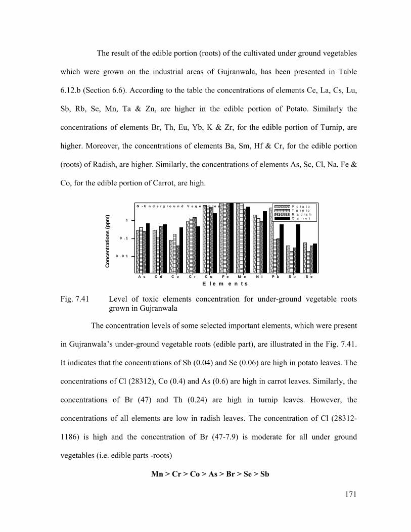
171
The result of the edible portion (roots) of the cultivated under ground vegetables
which were grown on the industrial areas of Gujranwala, has been presented in Table
6.12.b (Section 6.6). According to the table the concentrations of elements Ce, La, Cs, Lu,
Sb, Rb, Se, Mn, Ta & Zn, are higher in the edible portion of Potato. Similarly the
concentrations of elements Br, Th, Eu, Yb, K & Zr, for the edible portion of Turnip, are
higher. Moreover, the concentrations of elements Ba, Sm, Hf & Cr, for the edible portion
(roots) of Radish, are higher. Similarly, the concentrations of elements As, Sc, Cl, Na, Fe &
Co, for the edible portion of Carrot, are high.
A s C d C o C r C u F e M n N i P b S b S e
0 . 0 1
0 . 1
1
G - U n d e r g r o u n d V e g e t a b l e s
Co
nce
ntr
atio
ns
(pp
m)
E l e m e n t s
P o t a t o T u r n i p R a d i s h C a r r o t
Fig. 7.41 Level of toxic elements concentration for under-ground vegetable roots
grown in Gujranwala
The concentration levels of some selected important elements, which were present
in Gujranwala’s under-ground vegetable roots (edible part), are illustrated in the Fig. 7.41.
It indicates that the concentrations of Sb (0.04) and Se (0.06) are high in potato leaves. The
concentrations of Cl (28312), Co (0.4) and As (0.6) are high in carrot leaves. Similarly, the
concentrations of Br (47) and Th (0.24) are high in turnip leaves. However, the
concentrations of all elements are low in radish leaves. The concentration of Cl (28312-
1186) is high and the concentration of Br (47-7.9) is moderate for all under ground
vegetables (i.e. edible parts -roots)
Mn > Cr > Co > As > Br > Se > Sb

172
7.7. Comparison of crops, vegetables and soils with literature reference values
A comparison among the elemental values of present work for vegetables, crops
and soils with literature cited reference values is presented in this section. In this regard,
the values of selected trace elements in vegetables for such comparison are listed in Tables
7.2 to 7.4 and the values of selected trace elements in crops (wheat, rice, maize and millet)
for such comparison are listed in Tables 7.5a & b. Similarly, the values of selected trace
elements in soils for such comparison are listed in Table 7. 6.
A comparison is presented in Table 7.2 among the literature (Waheed, Singh &
Al-Jabori) cited values and present work for more than twenty-five selected (i.e. minor,
major, toxic, trace, etc) elements in each summer vegetable (i.e. brinjal, tomato and bitter
gourd), which were collected from both Faisalabad and Gujranwala industrial areas. In case
of brinjal, the concentrations (μg/g) of eleven elements (As, Cd, Ce, Co, Cr, Eu, La, Ni, Pb,
Sc and Se) out of 25 observed elements were 2-3 times high for present work as compared
to the literature reported values. The values of Br, Fe, Mn, Na, Sb and Zn are comparable
with each other while the values of Cl and K are very low as compared to the reported
values. In case of tomato, the concentrations (μg/g) of eleven elements (Br, Cd, Cu, Eu, Fe,
La, Mn. Ni, Pb, Sc and Se) out of 25 observed elements were more than two times high for
present work as compared to the literature reported values. Similarly, in case of bitter
gourd, the concentrations (μg/g) of ten elements (As, Ba, Co, Cr, Eu, Fe, La, Mn, Na and
Zn) out of 25 observed elements were 2-3 times high for present work as compared to the
literature reported values.

173
A comparison is presented in Table 7.3 among the literature cited values and
present work for more than twenty-five selected elements in each winter vegetable (i.e.
cabbage, spinach and potato), which were cultivated in both Faisalabad and Gujranwala
industrial areas. In case of cabbage, the concentrations of twelve elements (i.e. Ba, Ce, Cl,
Cr, Eu, Fe, La, Ni, Pb, Se and Th) were 2-3 times high for present work as compared to the
literature reported values. The values of Br, Fe, Mn, Na, Sb and Zn are comparable with
each other while the values of Cl and K are very low as compared to the reported values. In
case of spinach, the concentrations of seven elements (i.e. As, Cr, Eu, Fe, La, Se and Th)
were more than two times high for present work as compared to the literature reported
values. Similarly, in case of potato, the concentrations of eighteen elements (i.e. As, Ba, Br,
Ce, Cr, Cs, Eu, La, Mn, Ni, Pb, Sb, Sc, Se, Ta, Th, Tb and Zn) were 2-3 times high for
present work as compared to the literature reported values.
Table 7.4 represents the comparison among the literature-cited values and
present work for more than twenty-six selected elements in each under ground vegetable
(i.e. turnip, radish and carrot), which were cultivated in both Faisalabad and Gujranwala
areas. In case of Turnip, the concentrations of fourteen elements (i.e. As, Ce, Cr, Cs, Cu,
Eu, La, Mn, Ni, Pb, Ta and Zn) out of 26 observed elements were 2-3 times high for
present work as compared to the literature reported values. In case of radish, the
concentrations of fourteen elements (i.e. As, Ba, Cd, Cr, Cs, Cu, Eu, La, Ni, Pb, Sb, Se, Ta
and Yb) out of 26 observed elements were more than two times high for present work as
compared to the literature reported values. Similarly, in carrot, for present work, the
concentrations of seven elements (i.e. Br, Cd, Cr, Mn, Ni, Pb, and Zn) out of 26 observed
elements were 2-3 times high as compared to the literature reported values.

174
Table 7.2 A comparison between the trace elemental concentrations (μg/g) of literatures cited values and present work for summer vegetables (NR ≈ Not Reported)
Names/ Elements
Brinjal Tomato Bitter gourd
Faisalabad Gujranwala Reference values
Reference values
Faisalabad Gujranwala Reference values
Reference values
Faisalabad Gujranwala Reference values
Reference values
As 0.49±0.01 0.26±0.01 0.115±0.01130 NR 0.53±0.04 0.44±0.03 0.69±0.07130 NR 0.35±0.01 0.2±0.02 0.177±0.02130 NR
Ba 9.6±0.1 11.3±0.2 27.5±2.0130 NR 5.43±0.18 5.7±0.45 6.3±0.6130 31.9±4.498 72±4.0 53±3.0 43.6±3.8130 NR
Br 24.8±1.6 19.6±1.3 24.2±1.7130 47.5±1698 65±3.8 52±2.9 10.3±0.9130 NR 6.3±0.5 9.4±0.1 5.9±0.6130 35.267
Cd 0.08±0.001 0.09±0.001 0.07±0.00496 0.0793 0.08±0.002 0.1±0.01 NR 0.075±0.00396 0.05±0.001 0.07±0.001 0.0693 0.02567
Ce 0.76±0.1 0.88±0.01 0.65±0.06130 NR 0.16±0.01 0.22±0.01 0.38±0.03130 NR 0.5±0.01 0.26±0.01 0.86±0.07130 NR
Cl 982±31 547±56 6448±359130 650±8098 1279±74 698±61 2089±120130 11100±230098 1812±39 725±44 2328±108130 190067
Co 0.29±0.02 0.35±0.02 0.076±0.008130 0.12±0.0398 0.4±0.02 0.5±0.01 0.17±0.019130 0.43±0.1498 0.17±0.01 0.21±0.04 0.168±0.01130 0.0767
Cr 1.37±0.5 11.6±0.05 0.97±0.1130 6.1693 1.67±0.02 2.68±0.02 2.4±0.2130 0.11±0.00496 4.4±0.2 5.7±0.8 1.5±0.1130 0.4667
Cs 0.1±0.03 0.12±0.01 0.11±0.01130 NR 0.3±0.01 0.5±0.06 0.78±0.08130 NR 0.19±0.01 0.13±0.02 0.135±0.01130 NR
Cu 6.5±0.3 8.3±0.5 2.8±0.2130 13.3293 11.3±0.1 12.2±0.6 10.8±0.9130 NR 10.2±0.1 11.5±1.0 9.4±0.8130 13.793
Eu 0.02±0.001 0.03±0.002 0.004±0.0005130 NR 0.02±0.001 0.03±0.002 0.003±0.0003130 NR 0.09±0.003 0.08±0.001 0.019±0.002130 NR
Fe 587±21 651±27 95±7.0130 815±15.498 250±21 347±33 105±9.0130 238±18498 372±10 222±30 120±9.0130 20767
K 2871±303 2456±254 29000±2000130 15000±890098 5761±515 5622±364 28000±2000130 41600±110098 3325±457 3265±318 27000±2000130 2990067
La 0.3±0.01 0.1±0.01 0.012±0.002130 NR 1.48±0.26 1.3±0.2 0.995±0.018130 NR 0.6±0.06 0.8±0.07 0.01±0.002130 NR
Mn 11±1.2 9.0±0.03 13.6±0.6130 5.27±2.598 13±1.3 10±1.0 12.2±0.6130 11.6±2.798 38±2.6 45.3±2.0 17.4±0.8130 26.367
Na 1154±137 1036±83 1270±100130 1060±145098 1624±186 1596±118 1930±1000130 2850±54098 3987±154 3379±326 1470±100130 34067
Ni 1.6±0.1 2.1±0.1 0.08±0.00596 9.4893 1.5±0.1 1.9±0.1 NR 1.365±0.0196 2.3±0.1 3.1±0.1 8.3293 0.46100
Pb 0.8±0.01 0.9±0.01 0.06±0.00596 1.7893 0.3±0.01 0.5±0.01 NR 0.255±0.00396 1.1±0.1 1.7±0.1 2.1593 0.115100
Rb 6.1±0.2 5.1±0.1 10.2±0.8130 13.1±2.498 33.4±1.0 40±1.3 37.3±2.9130 16.9±3.398 10.2±0.1 9.4±0.3 27.3±0.293 8.167
Sb 0.03±0.001 0.05±0.004 0.068±0.007130 2.85±0.798 0.03±0.001 0.08±0.001 0.057±0.006130 NR 0.06±0.004 0.1±0.01 0.072±0.008130 0.04567
Sc 0.16±0.08 0.2±0.06 0.01±0.001130 NR 0.04±0.004 0.09±0.01 0.014±0.001130 NR 0.08±0.006 0.06±0.001 0.063±0.006130 0.00967
Se 0.24±0.01 0.29±0.08 0.028±0.003130 NR 0.11±0.05 0.18±0.02 0.039±0.004130 NR 0.08±0.001 0.1±0.01 0.034±0.003130 0.0667
Ta 0.3±0.01 0.14±0.01 0.9±0.09130 NR 0.5±0.01 0.7±0.01 0.58±0.05130 NR 1.1±0.1 2.02±0.01 2.6±0.2130 NR
Yb 0.12±0.01 0.16±0.04 0.94±0.08130 NR 0.6±0.01 0.9±0.01 2.5±0.2130 NR 1.3±0.1 1.05±0.1 1.7±0.1130 NR
Zn 34±3.0 35±4.0 39.5±3.6130 81.5±15.498 47.8±2.6 80±2.0 36.2±3.5130 91.3±10.398 111±2.0 99.8±7.0 71.3±6.2130 8167

175
Table 7.3 A comparison between the trace elemental concentrations (μg/g) of literatures cited values and present work for winter vegetables (NR ≈ Not Reported)
Names/ Elements
Cabbage Spinach Potato
Faisalabad Gujranwala Reference values
Reference values
Faisalabad Gujranwala Reference values
Reference values
Faisalabad Gujranwala Reference values
Reference values
As 2.73±0.34 1.9±0.1 0.15±0.016130 1.2101 0.52±0.02 0.94±0.06 0.198±0.02130 NR 0.36±0.02 0.3±0.01 0.21±0.02130 NR
Ba 23.7±1.6 19.7±0.48 7.8±0.7130 NR 10.5±1.1 15.2±0.1 10.5±1.0130 NR 8.9±0.3 7.9±0.2 5.9±0.6130 NR
Br 4.3±0.2 10.6±0.8 5.3±0.5130 6.4±4.968 32±1.6 26±1.9 28.1±1.3130 1667 11.4±0.9 7.9±1.0 1.3±0.1130 10.7±11.498
Cd 1.1±0.1 1.4±0.1 0.9±0.0496 1.5101 0.1±0.01 0.3±0.02 0.6±0.0196 0.0993 0.2±0.01 0.3±0.01 0.4596 NR
Ce 0.78±0.3 0.59±0.03 0.1±0.01130 NR 0.4±0.01 1.0±0.1 0.46±0.04130 NR 3.7±0.5 2.5±0.4 1.1±0.1130 NR
Cl 1438±136 1267±116 997±76130 1240±14098 6321±237 5248±253 5175±295130 771067 783±9.0 1186±82 953±79130 6700±140098
Co 0.25±0.01 0.19±0.01 0.06±0.006130 0.66±0.1498 0.11±0.03 0.46±0.03 0.223±0.02130 0.27767 0.1±0.01 0.08±0.002 0.08±0.007130 0.33±0.2898
Cr 1.4±0.52 1.05±0.05 0.47±0.05130 0.5±0.0298 2.8±0.1 3.8±0.1 2.3±0.2130 1.1767 1.3±0.3 0.96±0.01 0.8±0.09130 0.19±0.0198
Cs 0.02±0.006 0.02±0.001 0.59±0.006130 NR 0.1±0.03 0.3±0.01 0.29±0.03130 NR 0.9±0.1 0.68±0.02 0.53±0.05130 NR
Cu 8.1±0.7 9.1±0.8 7.4±0.5130 5.19±1.1104 21±1.2 27±2.1 30.4±2.3130 19.2293 4.8±0.2 7.1±0.3 6.9±0.5130 NR
Eu 0.01±0.001 0.02±0.001 0.005±0.001130 NR 0.4±0.02 0.7±0.01 0.16±0.018130 NR 0.01±0.003 0.007±0.0001 0.005±0.0005130 NR
Fe 172±11 279±13 89±7.0130 117±6898 389±26 441±72 363±22130 28867 63±7.0 82±5.0 68±5.0130 40±2598
K 1718±177 1136±124 12200±900130 32000±780098 3725±328 4832±261 25000±1300130 2540067 2593±362 23364±121 22000±1100130 24200±430098
La 3.79±0.1 2.1±0.1 1.4±0.1130 NR 0.1±0.01 0.3±0.02 0.018±0.002130 NR 3.6±0.3 2.3±0.2 1.14±0.1130 NR
Mn 13.7±1.4 10±0.1 8.9±0.4130 17.7±2.698 22±2.3 16±0.3 79±3.8130 23967 10.5±0.8 9.3±0.5 8.5±0.4130 5.85±2.198
Na 2732±343 2165±145 4250±300130 2630±99098 4893±316 4126±156 42000±3000130 932067 2166±113 1649±107 1380±100130 660±7298
Ni 1.1±0.1 1.8±0.1 NR NR 2.6±0.1 3.2±0.1 NR 18.5193 1.8±0.1 2.1±0.1 1.65596 NR
Pb 2.3±0.2 2.8±0.3 1.6101 NR 2.1±0.1 3.3±0.1 1.75±0.0896 7.3493 3.4±0.2 5.2±0.4 NR NR
Rb 2.85±0.84 3.1±0.2 9.8±0.5130 4.63±1.498 15.5±1.6 18.5±0.4 11.2±0.8130 16967 13±1.0 9.6±0.6 7.2±0.05130 17.7±2498
Sb 0.01±0.001 0.02±0.001 0.03±0.003130 NR 0.02±0.005 0.04±0.001 0.116±0.012130 0.01467 0.06±0.002 0.04±0.001 0.026±0.006130 NR
Sc 0.01±0.001 0.03±0.002 0.01±0.001130 NR 0.03±0.001 0.05±0.003 0.076±0.008130 0.02167 0.01±0.001 0.008±0.0007 0.007±0.0007130 0.08±0.0198
Se 0.09±0.008 0.06±0.002 0.03±0.004130 NR 0.06±0.002 0.08±0.005 0.016±0.002130 0.03967 0.1±0.02 0.06±0.005 0.05±0.006130 NR
Ta 0.28±0.04 0.3±0.03 0.69±0.05130 NR 0.7±0.02 0.5±0.08 1.2±0.1130 NR 3.4±0.2 3.0±0.2 1.0±0.08130 NR
Th 0.23±0.01 0.33±0.02 NR NR 0.26±0.01 0.37±0.03 NR 0.17967 0.04±0.001 0.1±0.01 NR NR
Yb 0.07±0.003 0.17±0.08 1.2±0.1130 NR 0.4±0.01 0.5±0.08 1.8±0.2130 NR 0.7±0.01 0.5±0.02 0.48±0.04130 NR
Zn 59±36 86±1.8 37.3±3.3130 70.4±8.698 42.2±1.8 56±3.0 42.2±3.3130 57.867 51±3.0 46±4.0 22.3±2.3130 16.2±8.598

176
Table 7.4 A comparison between the trace elemental concentrations (μg/g) of literatures cited values and present
work for underground vegetables (NR ≈ Not Reported)
Names/ Elements
Turnip Radish Carrot Faisalabad Gujranwala Reference
values Reference
valuesFaisalabad Gujranw
alaReference
values Reference
valuesFaisalabad Gujranw
alaReference
values As 0.22±0.02 0.4±0.02 0.12±0.01130 NR 0.43±0.05 0.26±0.02 0.13±0.01130 NR 0.73±0.01 0.68±0.05 NR Ba 27±4.0 5.2±0.4 16±1.4130 NR 23±4.0 11±1.0 9.3±1.0130 NR 13±1.0 8.0±0.1 NR Br 26±5.0 47±8.0 6.6±0.6130 40.2±16.498 19.9±1.3 15.2±2.0 7.7±0.6130 82.9±8498 35.8±3.1 27.8±2.4 26.5±15.998 Cd 0.09±0.001 0.12±0.001 0.115±0.00596 NR 0.4±0.01 0.5±0.01 0.35±0.0396 NR 0.4±0.01 0.51±0.02 0.32±0.0396 Ce 0.8±0.05 0.5±0.01 0.4±0.03130 NR 0.3±0.01 0.09±0.006 0.15±0.01130 NR 0.1±0.01 0.07±0.001 NR Cl 872±18 1132±24 697±43130 13500±140098 1287±15 1694±23 2223±129130 1400±40098 3267±44 28312±161 25000±960098
Co 0.3±0.04 0.18±0.01 0.2±0.02130 1.69±0.5698 0.07±0.003 0.04±0.004 0.049±0.006130 0.7±0.298 0.65±0.02 0.4±0.03 0.52±0.498 Cr 1.9±0.2 1.4±0.1 1.0±0.1130 0.39±0.0498 2.4±0.3 1.5±0.1 1.6±0.1130 0.35±0.0496 0.8±0.05 0.47±0.04 0.4±0.0398 Cs 0.2±0.01 0.6±0.02 0.1±0.01130 NR 0.22±0.03 0.08±0.001 0.1±0.01130 NR 0.14±0.01 0.05±0.001 NR Cu 4.7±0.2 5.8±0.3 3.3±0.2130 NR 4.1±0.2 5.3±0.4 3.2±0.3130 NR 2.1±0.1 2.5±0.1 NR Eu 0.01±0.002 0.008±0.0006 0.006±0.001
130 NR 0.01±0.001 0.009±0.0003 0.007±0.001130 NR 0.05±0.001 0.03±0.001 NR
Fe 121±6.0 94±8.0 96±7.0130 175±4198 110±4.0 120±7.0 137±9.0130 417±5798 123±6.0 136±4.0 135±58.598 K 2835±326 37569±428 23000±1000130 27400±630098 4649±245 33982±211 24000±5000130 39600±690098 3129±561 25664±123 24800±390098
La 0.05±0.004 0.07±0.001 0.05±0.005130 NR 0.06±0.001 0.04±0.001 0.02±0.003130 NR 0.4±0.01 0.3±0.01 NR Mn 6.9±0.4 8.4±0.7 6.4±0.3130 6.8±2.898 9.7±1.0 4.6±0.1 21.5±1.0130 3.76±1.598 8.3±0.1 5.7±0.1 4.52±2.598 Na 2366±141 6697±328 1060±100130 5010±125098 1669±129 3698±334 9560±500130 15600±320098 2236±151 9472±324 17600±140098
Ni 1.0±0.1 1.3±0.1 0.895±0.008130 NR 0.7±0.01 0.9±0.01 NR NR 2.1±0.1 3.2±0.2 1.985±0.00696
Pb 0.07±0.001 0.09±0.001 0.06±0.01130 NR 0.08±0.001 0.12±0.01 0.05±0.00196 NR 0.5±0.02 0.6±0.03 0.485±0.00596
Rb 29±3.0 25±1.0 28.3±1.9130 23±2098 10.6±0.5 8.8±0.3 8.8±0.8130 63.6±31.698 4.4±0.2 5.1±0.1 4.7±1.498 Sb 0.05±0.002 0.02±0.001 0.04±0.005130 NR 0.04±0.001 0.03±0.001 0.026±0.003130 NR 0.09±0.001 0.6±0.03 NR Sc 0.04±0.001 0.01±0.001 0.015±0.002
130 0.04±0.0198 0.02±0.001 0.02±0.002 0.02±0.002130 NR 0.06±0.001 0.05±0.002 0.03±0.0198
Se 0.05±0.002 0.02±0.001 0.02±0.002130 NR 0.03±0.001 0.04±0.001 0.013±0.001130 NR 0.02±0.001 0.03±0.002 NR Ta 1.6±0.1 1.3±0.1 1.1±0.1130 NR 1.0±0.1 0.8±0.06 0.87±0.09130 NR 0.3±0.01 0.17±0.01 NR Yb 1.1±0.1 1.6±0.1 2.2±0.1130 NR 1.9±0.1 1.3±0.1 1.1±0.1130 NR 0.8±0.02 0.5±0.05 NR Zn 42±2.0 40±1.0 38.9±3.1130 14.5±1.698 37±3.0 57±1.5 40.7±3.8130 74.5±8.498 20±1.0 19±1.0 13.4±3.498

177
Table 7.5.a Concentrations (g/g) of trace elements in wheat and rice crops (edible portion) along with their literature cited values (NR ≈ Not Reported)
Crops/ Elements
Faisalabad Wheat
Gujranwala Wheat
Reference values
Reference values
Faisalabad Rice
Gujranwala Rice
Reference values
Reference values
As 0.16±0.04 0.32±0.02 0.058±0.006130 0.13±0.09173 0.18±0.02 0.31±0.02 0.087±0.009130 0.2101 Ba 6.9±0.4 4.6±0.1 1.3±0.1130 NR 5.0±0.2 7.2±0.3 3.9±0.3130 NR Br 2.1±0.1 3.42±0.34 0.8±0.08130 0.6167 0.9±0.01 1.4±0.1 0.64±0.06130 1.9±0.2104 Cd 0.1±0.01 0.08±0.006 NR 0.18±0.07173 0.05±0.001 0.09±0.004 0.11±0.07171 0.025±0.004107 Ce 0.38±0.02 0.53±0.07 0.31±0.03130 NR 0.4±0.01 0.31±0.02 0.05±0.005130 NR Cl 846±31 277±44 924±73130 18067 399±28 357±13 269±17130 NR Co 0.018±0.003 0.04±0.003 0.014±0.002130 0.03567 0.1±0.01 0.11±0.01 0.31±0.04130 0.3±0.07104 Cr 0.7±0.04 0.39±0.01 0.2±0.02130 0.2167 1.7±0.3 0.65±0.08 0.43±0.04130 0.86±0.14104 Cs 0.04±0.001 0.09±0.005 0.07±0.008130 NR 0.01±0.005 0.026±0.002 0.06±0.006130 0.075±0.001107 Cu 14.2±1.2 15.5±1.6 3.6±0.2130 0.2367 8.1±1.0 9.9±1.1 4.9±0.4130 2.5±0.4104 Eu 0.02±0.001 0.1±0.01 0.05±0.006130 NR 0.01±0.003 0.06±0.001 0.05±0.006130 NR Fe 217±26 540±11 241±17130 18167 120±1.0 233.7±1.5 21.5±2.0130 63±4.8104 K 1292±102 1966±159 3400±200130 200067 2229±132 1642±30 1900±100130 830±20104 La 0.86±0.02 0.6±0.02 0.39±0.04130 NR 0.11±0.06 0.1±0.01 0.064±0.007130 NR Mn 33.7±2.6 40±3.0 16.2±1.2130 0.1967 9.9±0.2 8.65±0.3 8.6±0.4130 9.5±3.0104 Na 669±41 345±27 532±43130 2067 337±47 123±11.6 35±2.0130 110±30104 Ni 0.24±0.04 0.36±0.06 NR 1.49±0.88173 4.3±0.6 4.9±0.8 0.97±0.66173 0.67±0.36110 Pb 0.48±0.07 0.61±0.09 NR 0.86±0.79173 2.36±0.3 3.84±0.27 0.6±0.3171 1.5101 Rb 2.1±0.2 2.7±0.6 5.3±0.4130 6.3667 0.6±0.02 6.8±0.9 1.8±0.1130 1.6±0.38110 Sb 0.03±0.001 0.08±0.005 0.06±0.001130 0.19567 0.05±0.004 0.03±0.002 0.011±0.002130 0.066±0.003107 Sc 0.05±0.001 0.04±0.001 0.08±0.009130 0.00967 0.01±0.001 0.04±0.003 0.03±0.003130 NR Se 0.28±0.06 0.6±0.01 0.22±0.028130 0.12767 0.6±0.06 1.1±0.2 0.75±0.074130 0.26±0.03110 Ta 0.5±0.01 0.3±0.01 0.9±0.08130 NR 0.36±0.01 0.48±0.01 0.73±0.06130 NR Tb 0.6±0.01 0.2±0.01 1.1±0.1130 NR 0.51±0.01 0.4±0.01 0.85±0.08130 NR Th 0.05±0.002 0.08±0.002 NR 0.04367 0.42±0.01 0.57±0.01 NR NR Yb 1.4±0.05 1.2±0.01 1.1±0.1130 NR 0.81±0.01 0.69±0.05 0.94±0.08130 NR Zn 27±2.0 45.2±4.5 26.3±2.5130 28.567 48±4.1 22.3±3.9 18.7±1.9130 30.8±5.2104
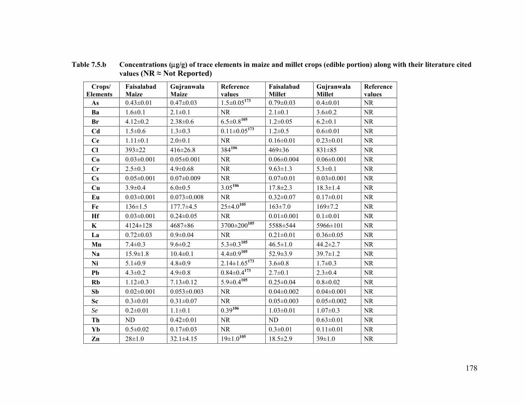
178
Table 7.5.b Concentrations (g/g) of trace elements in maize and millet crops (edible portion) along with their literature cited values (NR ≈ Not Reported)
Crops/ Elements
Faisalabad Maize
Gujranwala Maize
Reference values
Faisalabad Millet
Gujranwala Millet
Reference values
As 0.43±0.01 0.47±0.03 1.5±0.05173 0.79±0.03 0.4±0.01 NR
Ba 1.6±0.1 2.1±0.1 NR 2.1±0.1 3.6±0.2 NR
Br 4.12±0.2 2.38±0.6 6.5±0.8105 1.2±0.05 6.2±0.1 NR
Cd 1.5±0.6 1.3±0.3 0.11±0.05173 1.2±0.5 0.6±0.01 NR
Ce 1.11±0.1 2.0±0.1 NR 0.16±0.01 0.23±0.01 NR
Cl 393±22 416±26.8 384106 469±36 831±85 NR
Co 0.03±0.001 0.05±0.001 NR 0.06±0.004 0.06±0.001 NR
Cr 2.5±0.3 4.9±0.68 NR 9.63±1.3 5.3±0.1 NR
Cs 0.05±0.001 0.07±0.009 NR 0.07±0.01 0.03±0.001 NR
Cu 3.9±0.4 6.0±0.5 3.05106 17.8±2.3 18.3±1.4 NR
Eu 0.03±0.001 0.073±0.008 NR 0.32±0.07 0.17±0.01 NR
Fe 136±1.5 177.7±4.5 25±4.0105 163±7.0 169±7.2 NR
Hf 0.03±0.001 0.24±0.05 NR 0.01±0.001 0.1±0.01 NR
K 4124±128 4687±86 3700±200105 5588±544 5966±101 NR
La 0.72±0.03 0.9±0.04 NR 0.21±0.01 0.36±0.05 NR
Mn 7.4±0.3 9.6±0.2 5.3±0.3105 46.5±1.0 44.2±2.7 NR
Na 15.9±1.8 10.4±0.1 4.4±0.9105 52.9±3.9 39.7±1.2 NR
Ni 5.1±0.9 4.8±0.9 2.14±1.65173 3.6±0.8 1.7±0.3 NR
Pb 4.3±0.2 4.9±0.8 0.84±0.4173 2.7±0.1 2.3±0.4 NR
Rb 1.12±0.3 7.13±0.12 5.9±0.4105 0.25±0.04 0.8±0.02 NR
Sb 0.02±0.001 0.053±0.003 NR 0.04±0.002 0.04±0.001 NR
Sc 0.3±0.01 0.31±0.07 NR 0.05±0.003 0.05±0.002 NR
Se 0.2±0.01 1.1±0.1 0.39106 1.03±0.01 1.07±0.3 NR
Th ND 0.42±0.01 NR ND 0.63±0.01 NR
Yb 0.5±0.02 0.17±0.03 NR 0.3±0.01 0.11±0.01 NR
Zn 28±1.0 32.1±4.15 19±1.0105 18.5±2.9 39±1.0 NR

179
A comparison is presented in Table 7.5a&b among the literature cited values
and present work for more than twenty-five selected (i.e. minor, major, toxic, trace, etc)
elements in each crop (i.e. wheat, rice, maize and millet), which were grown in Faisalabad
and Gujranwala areas. In case of wheat, the concentrations (μg/g) of eleven elements (As,
Ba, Br, Ce, Cr, Cu, La, Mn, Se, Th and Yb) out of 27 observed elements were 2-3 times
high for present work as compared to the literature reported values. The values of Br, Fe,
Mn, Na, Sb and Zn are comparable with each other while the values of Cl and K are very
low as compared to the reported values. In case of rice, the concentrations (μg/g) of nine
elements (Br, Ce, Cl, Cu, Fe, La, Na, Ni and Pb) out of 27 observed elements were more
than two times high for present work as compared to the literature reported values.
Similarly, in case of maize, the concentrations (μg/g) of eight elements (Cd, Cu, Fe, Mn,
Na, Ni, Pb and Zn) out of 28 observed elements were 2-3 times high for present work as
compared to the literature reported values.
Similarly, in Table 7.6 there is a comparison of concentrations of selected
elements present in soils, which were collected from Faisalabad and Gujranwala areas, with
literature values. It was observed that the concentrations of most of the elements were high
due to the mixing of industrial effluents with soil.

180
Table 7.6 Concentrations (g/g) of trace elements in the industrial soils along with their literature cited values
Places/ Elements
Faisalabad Soil
Gujranwala Soil
Reference values
Reference values
As 13.55±0.1 18.7±0.72 18.17±1.2441 13.3±4.0164 Ba 457±5.0 216±3.7 838±35.541 226112 Br 3.42±0.39 6.9±0.3 1.85±0.1141 6.7±1.8164 Cd 1.32±0.2 1.68±0.04 1.212 NR Ce 61±1.0 52.1±1.8 41.6±2.741 43.5±5.5174 Cl 867±111 512±17 732±12441 3620±800174 Co 7.8±0.1 16.5±0.4 23.86±1.0141 10±1.0174 Cr 138±1.0 86±0.8 85.83±3.1241 152±38174 Cs 5.02±0.2 5.24±0.5 13.85±0.6141 4.612 Cu 41±2.7 19.5±1.2 29.15±4.841 21.1±2.2174 Eu 0.85±0.06 0.92±0.07 0.69±0.0741 NR Fe 21293±328 19855±118 38800±70041 27000±200174 Hf 5.07±0.3 8.4±0.1 2.85±0.1741 10.6±1.4174 K 20852±516 33483±276 23000±110041 2810±596174 La 29.4±0.4 41±2.0 32.55±2.0341 21.6±0.9174 Mg 4572±83 3658±79 666±12241 410512 Mn 544±5.2 320±4.9 1360±10041 378±49174 Na 3941±258 2168±20.4 4200±20041 822±185174 Ni 32±1.5 33±1.1 43.912 12.5±3.0174 Pb 53±2.2 74±3.2 NR 85.9±17.7174 Rb 94±2.0 112±19.6 100±3.541 34.8±2.3174 Sb 1.69±0.05 1.11±0.1 2.4±0.141 1.3±0.1174 Sc 7.0±0.1 8.1±0.5 12.13±0.941 4.9±0.1174 Se 3.28±0.7 1.76±0.05 1.3±0.141 3.8±0.8174 Th 11.88±0.7 13.88±1.12 6.512 6.0±0.8174 Ti 1542±78 1746±84 145012 3987±518174 V 101±1.2 93±1.1 12012 NR Yb 2.07±0.1 3.34±0.08 2.24±0.1241 2.5±0.5174 Zn 82±11 50.6±0.9 66.07±2.7241 72.7±9.7174 Zr 380±6.0 268±6.3 36012 507±168174
It may be concluded that the water resources contaminated with untreated
industrial effluents is cultivating fields around the industrial estates of Gujranwala and
Faisalabad.

181
CHAPTER-8
8. CONCLUSIONS AND RECOMMENDATIONS
Some salient findings and suggestions are described here as follows:
8.1. Conclusions:
The results of effluents for trace elemental concentrations and physico-chemical
analysis revealed that all untreated industrial effluents contain high concentrations of heavy
and toxic metals. Chemical analysis showed the nature of the industrial effluents. Effluents
vary in quality for textile, pulp, and ceramics industries and have specific nature for each
industry. These effluents have been treated, on laboratory scale, for the successful removal
of chromium, arsenic and iron by the use of UMFT unit and the column chromatography
through sweet peanut husk. According to the presence of high concentrations of pollution
parameters, the effluents of textile/ yarn industries were worse as compared to the effluents
of pulp/ paper and ceramics industries.
Textile/ Yarn Pulp/ Paper Ceramics
The soils cultivated with industrial effluent have comparatively higher pH and
EC values as relative to the soils irrigated from tube-well or canal water. High pH value is
not appropriate for growth of most of the crops and vegetables. High values of EC pointed
out the presence of alkali and alkaline earth metals in the soil, which hinder the growth of
plants. Similarly, the soils of industrial areas were with higher concentrations of the heavy
metals than the soils of non-industrial zones. Leaching tendency of some selected trace
elements in soils was also observed. The elements (Ba, Cr, As, Na, Cl, K, Br & Mg)
leached from topsoil to sub-soil very easily as compared to others (Mn, Sb, Sc, Co, Se, Fe

182
& Zn). The addition of different metal ions in cereals and vegetables is linearly linked to
the cumulative metal loading rate in soil due to the physical, chemical, mineralogical and
biological properties of the soils. However, the toxic elemental level is higher in the soil of
Faisalabad industrial areas as compared to that of Gujranwala.
Faisalabad Gujranwala
The diversity of metal ions uptake by plants (vegetables & cereals) not only
differs from species to species and morphology of soil but also due to climatic variations.
The obtained data from the present research to evaluate the levels of essential and toxic
trace elements in vegetables/ cereals will assist to identify the trends and sources of
pollution. It may be useful for regulatory authorities in the formulation of legislation
concerning the controlled release of industrial effluents into the environment. The normal
trend shows that the maximum concentration of the trace elements is accumulated in roots
while their least concentration is present in fruits i.e. edible part of cereals and vegetables.
Roots Stems Leaves Fruits (edible part)
The toxic activity reduces in the following sequence, which indicates wheat crop
is the least affected by the industrial effluents as compared to the other cereal crops.
Millet Maize Rice Wheat
It was observed that the concentrations of all elements are high in the wheat,
rice and vegetables grown in the industrial areas of Faisalabad & Gujranwala and low in
the non-industrial areas of Kashmir & Islamabad. The order of toxicity is as following:
Faisalabad Gujranwala Islamabad Kashmir
It is concluded that the crops and vegetables, cultivated with untreated effluents,
should not be utilized because such foods may have some adverse effects on the animals
183
and human health, through the accumulation of heavy metals poisoning into the bodies.
However, diet samples analyzed were not contaminated with trace toxic metals up to an
extent to cause any possible adverse impact on human health.
8.2. Recommendations:
The source of trace metal distribution is a pre-requisite to ensure the
quality of foodstuffs. Therefore, a regular monitoring of toxicity should be
conducted.
In industrial polluted areas the intake of Chlorine from the dietary items is
very low. So the chlorination of water should necessarily be done to meet
the required intake suggested by DRI.
The government has to ensure that all new and existing industries have
adequate sites facilities for treatment and removal of toxic materials from
the waste or effluents. Under no circumstances, the direct discharge of the
industrial effluents ought to be allowed in the stream or river. The
government should strictly enforce the existing pollution laws.
A public awareness campaign about the pollution should be launched with
strong emphasis on the effects of pollution on personal and community
health. Industrial pollution information must be published by
environmental public organizations periodically and using mass media for
informing the public sectors by utilizing audio and video media, holding
workshops, seminars, colloquia and presentations by the experts.

184
References
Sr. No. References
1. Connell, D.W., Basic concepts of environmental chemistry, Chapter-20 (Ecotoxicology - the interaction of chemicals with ecosystems), Lewis publishers, New York, USA, (1997) 459-467.
2. Hussain, M., Environmental degradation, realities and remedies, Chapter 6, Industrial Pollution, Feroz sons Ltd., Rawalpindi, Pakistan, (1998) 120-136.
3. Tchobanoglous, G., Burton, F.L., Waste water Engineering, treatment, disposal and reuse, Mc Grew-Hill, Inc, New York, 3rd Revised Edition, 1991.
4. National Environmental Quality Standards (NEQS), Pakistan environmental protection act, PEPA-97, The gazette of Pakistan 1997.
5. Welz, B., Sperling, M., Atomic Absorption Spectrometry, Wiley-VCH, New York, 3rd Revised Edition, 1999.
6. Svehla, G., Vogel’s Qualitative inorganic analysis, 7Th Edition, (2002) Pearson Education PTE Ltd, India
7. Mohammad, M., Electro analytical techniques: their scope and limitation in environmental analysis, The Nucleus, 36 (3-4), (1999) 125-136.
8. Lancaster, H.L., Marshall, G.D., Gonzalo, E.R., Ruzicka, J., Christian, G.D., Trace metal atomic absorption spectrometric analysis utilizing sorbent extraction on polymeric-based supports and renewable reagents, The Analyst, 119(7) (1994) 1459-1465.
9. Miyamoto, Y., Habra, H., Kalikow, A., Masumoto, K., Nakanishi, T., Sakamoto, K., Interferences in Neutron and Photon Activation Analysis, J. Radio anal. Nucl. Chem., 240 (1999) 165-175.
10. Bruin, M. de., Present and Future of Neutron Activation Analysis, J. Radio anal. Nucl. Chem. (Articles), 160 (1) (1992) 31-40.
11. Guinn, V.P., Past, Present and Future of Neutron Activation Analysis, J. Radio anal. Nucl. Chem. (Articles), 160 (1), (1992) pp 09-19.
12. Neumann, R., Steinnes, E., Guinn, V. P., Feasibility of instrumental neutron activation analysis for trace element studies in natural soils, J. Radio anal. Nucl. Chem. (Articles), 168 (1), (1993) 61-68.
13. Nasir, A., Practical considerations in instrumental neutron activation analysis, The Nucleus, 38 (3-4), (2001) 215-230.
14. Grazman, B.L., Schweikert, E.A., A brief review of the determination of Cadmium by Prompt Gamma-ray Neutron Activation Analysis (PGNAA), J. Radio. Anal. and Nucl. Chem. (Articles), 152(2), (1991) 497-506.
15. Kilikoglou, V., Grimanis, P., Vassilaki-Grimani, M., Grimanis, A. P., Comparison between two INAA methods applied to chemical characterization of ancient Ceramics, J. Radio anal. Nucl. Chem. (Articles),

185
151 (2), (1991) 469-477.
16. Freitas, M.C. Martinho, E., Accuracy and Precision in Instrumental Neutron Activation Analysis of Reference Materials and Lake Sediments, Analytica Chimica Acta., 223 (1), (1989) 287-292.
17. Gilmore, G., Hemingway, J., Practical Gamma ray Spectrometry, Chapter 5, “Statistics of Counting,” John Wiley & Sons, New York., (2004) 104-127.
18. Trkov, A., Nuclear reactions and physical models for neutron activation analysis, Lecture materials for the workshop on nuclear data for activation analysis, International center for theoretical physics, Miramare-Trieste, Italy, (2005)
19. Al-Bedri, M.B.H, Al-Jobori, S., Multi-element Determination in River Water By Neutron Activation Analysis, Journal of Radio-analytical and Nuclear Chemistry (Articles) 147(2) (1991) 235-241.
20. Alvarez, J. R. E., Montero, A. A., Jiménez, N. H., Muñiz, U. O., Padilla, A.R., Molina, R. J., Vera, S. Q. D., Nuclear and related analytical methods applied to the determination of Cr, Ni, Cu, Zn, Cd and Pb in a red ferralitic soil and Sorghum samples, J. Radio anal. Nucl. Chem., 247 (3) (2001) 479-486.
21. Be-dregal, P.S., Montoya, E.H., Determination of Cadmium using Radio-chemical Neutron Activation Analysis, Journal of Radio-analytical and Nuclear Chemistry, 254 (2), (2002) 363-364.
22. Ehmann, W. D., Vance, D. E., Studies of trace element involvement in human disease by in vitro activation analysis, (Medical and Industrial Application), J. Radio anal. Nucl. Chem. (Articles), 203 (2), (1996) 429-445.
23. Bode, R.M.W.P., Goeij, J.J.M., Hoogenboom, J.E., Feasibility of elemental analysis of kilogram size samples by Neutron Activation Analysis, Anal. Chem., 68 (1996), 341-348.
24. Dardenne, C., Deschanps, N., Revel, G., Riglet, G., Herviou, C., Application of the K0 standardization method in Neutron Activation Analysis of ceramic materials, J. Radio anal. Nucl. Chem. (Articles), 168 (2) (1993) 417-427.
25. Freitas, M.C. Martinho, E., Neutron Activation Analysis of Reference Materials by the Co-Standardization and Relative Methods, Analytica Chimica Acta., 219 (2) (1989) 317-322.
26. Glasgow, D. C., Dyer, F. F., Robinson, L., Methods for preparing comparative standards and field samples for neutron activation analysis of soil, J. Radio anal. Nucl. Chem. (Articles), 192 (2), (1995) 361-370.
27. Over-water, R. M. W., Bode, P., Goeij, J. M. D., Hoogenboom, J. E., Feasibility of elemental analysis of kilogram-size samples by instrumental neutron activation analysis, Anal. Chem., 68 (1996) 341-348.
28. Kucera,-J., Selected industrial and environmental applications of neutron activation analysis, Workshop on industrial and environmental applications of nuclear analytical techniques, IAEA, Vienna (Austria) , Report of the workshop (1999) 117-129, 50 refs, 4 tables, IAEA-TECDOC—1121.

186
29. Fang, Z., Guo, T., Welz, B., Determination of cadmium, lead and copper in water samples by flame atomic-absorption spectrometry with pre-concentration by flow-injection on-line sorbent extraction, Talanta, 38(6) (1991) 613-619.
30. Hodrejarv, H.; Vaarmann, A., Pseudo-total analysis for metallic elements in siliceous soil by acid digestion and flame atomic absorption spectrometry, Analytica Chimica Acta, 396(2-3) (1999), 293-301.
31. Krekler, S., Frenzel, W., Schulze, G., Simultaneous determination of iron(II)/ iron(III) by sorbent extraction with flow-injection atomic absorption detection, Analytica Chimica Acta, 296(2) (1994) 115-117.
32. Ibrahim, M., Salmon, S., Chemical composition of Faisalabad city sewage effluent: I-Nitrogen, phosphorus and potassium contents, Pak. J. Agriculture Sci., 30 (1992 a) 381-390.
33. Ibrahim, M., Salmon, S., Chemical composition of Faisalabad city sewage effluent: II-Irrigation quality, J. Agriculture Res., 30 (1992 b) 391-401.
34. Ghafoor, A., Rauf, A., Arif, M., Muzaffar, W., Chemical composition of effluents from different industries of Faisalabad, Pak. J. Agriculture Sci., 31 (1994) 367-370.
35. Khan, A., Ibrahim, M., Ahmad, N., Anwar, S.A., Accumulation of heavy metals in soil receiving sewage effluent, J. Agricul. Res., 32 (1994) 525-533.
36. WHO (World Health Organization), Guidelines for drinking-water quality, Health Criteria and other supporting information, 1996, 94/9960-Mastereom/ Wiener Verlag-800, Australia.
37. WHO (World Health Organization), Trace elements in human nutrition, 1990, WHO, Technical report series No. 797, Geneva
38. World health organizations report WHO/FAO/IAEA., Expert consultation on trace elements in human nutrition and health, 1994; WHO, Geneva.
39. Ziai, K.H., Control and incentives for industrial waste water treatment and emerging waste water treatment practices in Pakistan, The Environ Monitor, 11 (3), (2002) 24 – 31.
40. Misra, R. N., Behera, P. K., The effect of Paper industry effluent on the growth, pigments, carbohydrates and proteins of Rice seedlings, Environmental Pollution, 72 (1991) 159-167
41. Reddy, A. V. R., Reactor neutron activation for multi elemental analysis,
Workshop on industrial and environmental applications of nuclear analytical techniques Vienna (Austria), Report of the workshop (1999) 129-145, 20 refs, 9 tables, IAEA-TECDOC—1121, AN: 30-060369
42. Ali, J., Javaid, M.A., Accumulation and distribution of Cd and Pb in sewage effluent irrigated soils, J. Eng. Appl. Sci., 16(1) (1997) 43-47.
43. Adhikari, S., Gupta, S.K., Banerjee, S.K., Heavy metals content of city sewage and sludge, J. Indian Soc. Soil Sci., 41 (1993) 170-172.

187
44. Manzoor, S., Munir, H.S., Shaheen, N., Khalique, A. Jaffar, M., Multivariate analysis of trace elements in textile effluents in relation to soil and ground water, Journal of hazardous materials, 137 (1) (2006) 31-37.
45. Kazmi A.M., Sacrificial Ion Exchange - A revolution in waste water treatment, The Environ Monitor, V I (12), (2001) 22-25.
46. Mann, J. G., Liu, Y. A., Industrial water reuse and waste water minimization, Chapter-4 (The design of distributed effluent treatment systems), Mc Grew Hill, New York, (1999) 77-122.
47. Mitchenko, T.; Stender, P.; Makarova, N., Optimization of sorption purification of industrial effluents, waste waters and technological solutions from polyvalent metal ions, Solvent extraction and ion exchange, 16 (1), (1998) 75-149.
48. Wells, M. J. M., Rossano, A. J., Roberts, E., Solid phase extraction for toxicity reduction evaluations of industrial waste-water effluents, Anal. Chim. Acta, 236 (1), (1990) 131-139.
49. Ghoreishi, S.M., Haghighi, R., Chemical catalytic reaction and biological oxidation for treatment of non-biodegradable textile effluents, Chemical Engineering Journal, 95 (1-3) (2003) 163-169.
50. Gianiuca Clardelli, Nicola Ranieri, The treatment and reuse of waste water in the textile industry by means of ozonation and electroflocculation, Water Research, 35 (2) (2001) 567-572.
51. Azbar, N., Yonar, T., Kestioglu, K., Comparison of various advanced oxidation processes and chemical treatment methods for COD and colour removal from a polyster and acetate fibre dyeing effluent, Chemosphere, 55 (1) (2004) 35-43.
52. Iyengar, G.V., Wolf, W.R., Tanner, J.T., Morris, E.R., Electrochemical coagulation for textile effluent decolorization, Journal of hazardous Materials, 127 (1-3) (2005) 40-47.
53. Garcia, J.C., Oliveria, J.L., Silva, A.E.C., Oliveria, C.C., Nozaki, J., de Souza, N.E., Comparative study of the degradation of real textile effluents by photo-catalytic reactions, Journal of Hazardous Materials, 147 (1-2) (2007) 105-110.
54. Chakzaborty, S., De, S., Basu, J.K., Das Gupta, S., Treatment of textile effluent: Application of a combination method involving adsorption and nanofiltration, Desalination, 174 (1) (2005) 73-85.
55. Selma Babursah, Mehmet Cakmakci, Cumali Kinaci, Analysis and monitoring: Costing textile effluent recovery and reuse, filtration and separation, 43 (5) (2006) 26-30.
56. Ona Gyliene, Sigita Visniakova, Heavy metal removal from solutions using natural and synthetic sorbents, Environmental research,engineering and management, 43(1) (2008) 28-34.
57. Nasim, A.K, Shaliza, I., Subramaniam, P., Elemination of heavy metals from waste water using agricultural wastes as adsorbents, Malaysian Journal of

188
Science, 23 (2004) 43-51.
58. Adam, F., Kandasamy, K., Balakrishnan, S., Iron incorporated heterogeneous catalyst from rice husk ash, Journal of colloidal and interface science, 304 (1) (2006)137-143.
59. Abdul-Ghani, N.T., Hefny, M., El-Chaghaby,G.A.F., Removal of lead from aqueous solution using low cost abundantly available adsorbents, Int. J. Environ. Sci. Tech., 4 (1) (2007) 67-73.
60. Srivostava, V.C., Mall, I.D., Mishra, I.M., Optimization of parameters for adsorption of metal ions on to rice husk, Chemical Engineering Journal, 140 (1-3) (2008) 136-144.
61. Cruvinel, P. E.; Flocchini, R. G.; Artaxo, P.; Crestana, S.; He., Elemental analysis of agricultural soil samples by particle induced x-ray emission (PIXE) technique, Nuclear Instrument Methods in Physics Research Section B – beam interactions with materials and A, 150 (1-4), (1999) 478-483.
62. Nabi, G., Ashraf, M. Aslam, M. R., Heavy metal contamination of agricultural soils irrigated with industrial effluents, Science Technology & Development, 20 (1), (2001) 32-36.
63. Kakar, R.G., Yasinzai, M., Salarzai, A.U. Nasir, M.H., Concentration of heavy metals in soil and spinach irrigated with sewage water in Quetta city, The Environ. Monitor, 12 (2005) 41-45.
64. Misra, S.G., Mani, D., Soil Pollution, Ashish Publishing House, 8/81, Punjabi Bagh, New Delhi, India, (1991) 109-110.
65. Farid, S., City effluent the major source of soil pollution, The Environ Monitor, 12, (2003) 23-25.
66. Ghafoor, A., Rauf, A., Muzaffar, W., Irrigation with Madhuana drain water: Impacts on soils and vegetables at Faisalabad, J. Drainage and Reclamation, 7 (1995) 7-12.
67. Singh, B., Singh, A.K., Natural radioactivity measurements in soil samples from some areas of Punjab and Himachal perdesh, India using gamma spectroscopy, Radiat. Meas., 39 (2004) 431-439.
68. Auburn, A. L., Heavy metal soil contamination, NRCS Urban technical note No. 3, (2000) 1-7.
69. Banuelos, G.S. Ajwa, H.A., Trace elements in soils and plants, J. Environ. Sci. Health-A, 34 (4) (1999) 951-974.
70. Chen, T.B., Wong, J.W.C., Zhou, H.Y. Wong M.H., Assessment of trace metal distribution and contamination in surface soils of Hong Kong, Environ. Pollut., 96 (1997) 61-68.
71. Chlopecka, A., Bacon, J. R., Wilson, M. J., Kay, J., Form of cadmium, lead and zinc in contaminated soils from south-west Poland, J. Environ. Qual., 25 (1996) 69-79.

189
72. Ebaid, Y, Y., El-Tahaway, M. S., El-Lakany, Garcia, S. R., Brooks, G.H., Environmental radioactivity measurements of Egyptian Soils, J. Radio. Anal. Nucl. Chem., 243 (2) (2000) 543-550.
73. Fresquez, P.R., Francis, R.E., Dennis, G.L., Sewage sludge effects on soil and plant quality in degraded semiarid grassland, J. Environ. Qual., 19 (1990) 324-329.
74. Giusquiani, P.L., Gigliotti, G., Businelli, D., Mobility of heavy metals in urban waste-amended soils, J. Environ. Qual., 21 (1992) 330-335.
75. Guengoer N, Alemdar A. Determination of trace elements by instrumental neutron activation analysis in Anatolian bentonitic clays, NIMB, Beam interactions with materials and atoms, 142 (4), (1998), 555-560.
76. Geiger, G., Federer, P., Sticher, H., Reclamation of heavy metal-contaminated soils: Field studies and germination experiments, J. Environ. Qual., 22 (1993) 201-207.
77. Holmgren, G. G. S., Meyer, M. W., Chaney, R. L., Daniels, R. B., Cadmium, lead, zinc, copper and nickel in agricultural soils of the United States of America, J. Environ. Qual., 22 (1993) 335-348.
78. Shtangeeva I.V., Vuorinen, A., Rietz, B., Christiansen, G., Carlson, L., Decontamination of polluted urban soil by plants. Our possibilities to enhance the uptake of heavy metals, J. radio. Anal. Nucl. Chem. (Articles), 249 (2) (2001) 369-374.
79. Sparks, D.L., Environmental soil chemistry, Academic Press, San Diego. CA, USA. (1995) 236-312.
80. Sterckeman, T., Douay, F., Priox, N. Fourrier, H., Vertical distribution of Cd, Pb and Zn in soils near smelters in the North of France, Environ. Pollut. 107 (2000) 377-389.
81. Winegardner, D. L., An introduction to soil for environmental professionals, Chapter 8, “Soil sampling techniques”, pp 147-159, 1995, Lewis Publishers, New York.
82. Wyttenbach, A., Tobler, L., Furrier, V., Schleppi, P., Variation of the rare earth element concentrations in the soil, soil extract and in individual plants from the same site, J. radio. Anal. Chem. (articles), 231 (1-2) (1998) 101-106
83. Lee, B. D., Carter, B. J., Basta, N. T., Weaver, B., Factors influencing heavy metal distribution in six Oklahoma benchmark soils, Soil Sci. Soc. Am. J., 61 (1997) 218-223.
84. Mc. Bride, M.B., Environmental chemistry of soils, Oxford Univ. Press, NY, USA, (1994) 127-213.
85. Mench, M.J., Didier, V.L., Loffler, M., Gomes, A., Masson, P., A mimicked in-situ remediation study of metal-contaminated soils with emphasis on cadmium and lead, J. Environ. Qual., 23 (1994) 58-63.
86. Ghafoor, A., Ahmad, S., Qadir, M., Murtaza, G., Movement and retention of

190
lead and chromium in soil applied with irrigation water, J. Arid Land Studies, (1999) 8-14
87. Murtaza, G., Ghafoor, A., Qadir, M. Rasheed, M. K., Concentration of Cd, Co and Mn in soils and vegetables irrigated with city effluent, National seminar on “Drainage in Pakistan”, Jamshoro, (2000) 177-182.
88. Javaid, M.A., Javaid, M., Heavy metal distribution and soil depth relation in some contaminated soil profile, J. Eng. Appl. Sci., 16(2), (1997) 59-64.
89. Kashem, M.A. Singh, B.R., Heavy metal contamination of soil and vegetation in the vicinity of industries in Bangladesh, Water, Air and Soil Pollution, 115 (1999) 347-361.
90. Nisar, A., Ibrahim, M., Khan, A., Long term disposal of city sewage effluent on agricultural lands: I-Effect on spinach growth, J. Agriculture Res., 32 (1994) 403-410.
91. Atta, S., Sattar, A., Ahmed, T., Sattar, S., Shamsuz-Zuha, Heavy metal contamination of vegetables grown on sewerage and canal water, J. Pure and Applied Sci., 16 (1997) 71-75.
92. Khan, A.S., Tabassum, R., Yousaf, M., Mineral elements of some green vegetables, J. Sci. & Tech. Univ. Peshawar, 22(1-2), (1998), 05-08.
93. Qadir M, Ghafoor A, Murtaza G., Irrigation with city effluent for growing vegetables: A silent epidemic of metal poisoning. Proceedings of Pak Acad Sci 36(2) (1999) 217-222.
94. Ado-Ekiti, S.S. Asaolu, Lead Content of Vegetables and Tomatoes at Erekesan Market, Pak. J. Sci. Ind. Res., 38 (11-12), (1995) 399-401.
95. Boon, D.Y., Soltanpour, P.N., Lead, cadmium and zinc contamination of Aspen Garden soils and vegetation, J. Environ. Qual. 21 (1992) 82-86.
96. Masud K, Jaffar M., Selected trace metal levels in local vegetables procured from Punjab, Pakistan, J Chem Soc Pak., 19(1) (1997) 49-53.
97. Husaini, S.N., Zaidi, J.H., Khan, E.U., Arif, M., Fatima, I., Qureshi, I.E., Malik, F., Arif, M., A study of polluted eco-system around industrial areas, Proc. Int. Conf. Environ. Sustainable Develop, Pakistan, III (2005) 1955-1962.
98. Al-Jabori, S.M., Itawi, R.K., Jalil, M., Saad, A., Ali, Kh.E., Determination of major, minor and trace elements in Iraqi vegetable samples by INAA, J. Radio anal. Nucl. Chem. (Articles), 159 (1) (1992) 29-36.
99. Fidanza, A. A., Burini, G., Perriello, G., Fidanza, F., Trace element intake and status of Italian subjects living in the Gubbio area, J. Environmental Research, 91 (2003) 71-77.
100. Gzyl, J., Lead and Cadmium contamination of soil and vegetables in the upper Silesia region of Poland, The science of the total environment, 96, (1990) 199-209.
101. Haiyan, W. Stuanes, A.O., Heavy metal pollution in air-water-soil-plant system of Zhuzhou city, Hunan province, China, Water, Air and Soil Pollution, 147

191
(2003) 79-107.
102. Phukan, S. Bhattacharya, K.G., Modification of soil quality near pulp and paper mill, Water, Air and Soil Pollution, 146 (1-4) (2003) 319-333.
103. Fardy, J. J., Mc Orist, G. D., Farrar, Y. J., The determination of Manganese status in the Australian diet using Neutron Activation Analysis, J. Radio anal. Nucl. Chem. (Articles), 163(2), (1992) 195-203.
104. Ahmad, S.A. Rizvi, R., Toxic effects of vegetables grown by city effluents on human health, The Environ. Monitor, 12 (2003) 21-22.
105. Khurshid, S. J., Waheed, S., Ahmad, S., Qureshi, I. H., Bio-availability of zinc from different Pakistani cereal grains, Specialist, Pak. J. Med. Sci., 15 (3 (1999) 225-228.
106. Armelin, M.J.A., Maihara, V.A., Vasconcellos, M.B.A., Favaro, D.I.T., Nascimento, V.F., Neutron activation analysis of the distribution of inorganic elements among five varieties of Brazilian Corn, J. Radio anal. Nucl. Chem., (Letters), 164 (4) (1992) 265-274.
107. Jibang, T., Qingfang, Q., Chifang, C., Wang, Ke., Tong, Qu., The distribution of Selenium and other elements in Corn samples studied by NAA and a biochemicacal technique, J. Radio anal. Nucl. Chem., (Articles), 151 (2), (1991) 287-292.
108. Mannan, A., Waheed, S., Qureshi, I. H., Concentration and distribution of toxic elements in Rice and Husk, J. Radio anal. Nucl. Chem. (Articles), 140 (1) (1990) 91-102.
109. Granato, T. C., G. R. Richardson, R. I. Pietz, C. Lue-Hing, Prediction of phytotoxicity and uptake of metals by models in proposed USEPA 40 CFR Part 503 sludge regulations: Comparison with field data for corn and wheat. Water, Air and Soil Pollution. 57-58 (1991) 891-902.
110. Hooda PS, Alloway BJ. The plant availability and DTPA extractability of trace metals in sludge-amended soils, Sci Total Environ 149 (1994a) 39-51.
111. Teherani, D.K., Trace elements analysis in Rice, J. Radio anal. Nucl. Chem., (Letters), 117 (3), (1987) 133-143.
112. Rubio, A. M., Salvador, A., Guardia, M. De ta., Ros, R., Determination of Cd and Ni in Rice plants by Flame Atomic Absorption Spectrometry, Atomic Spectroscopy, 14 (1), (1993) 08-12.
113. Waheed, S., Zaidi, J. H., Ahmad, S., Instrumental Neutron Activation Analysis of 23 individual food articles from a high altitude region: II. Determination of toxic trace elements, J. Radio Anal. Nucl. Chem., 254 (3) (2003) 73-81.
114. Ahmad M., Hussain, M., Shafique, M., Important Macro and Micro elements of Wheat and Rice, The Nucleus, 38 (3-4), (2001) 311-315.
115. Ahmed, S., Waheed, S., Mannan, A., Fatima, I., Qureshi, I.H., Evaluation of trace elements in wheat and wheat by products, J. Am. Oil Chem.(AOAC) International Soc., 77(1) (1994) 11-18.

192
116. Pulhani V. A., Dafauti, S., Hegde, A. G., Sharma, M. R., Mishra, U. C., Uptake and distribution of natural radioactivity in wheat plants from soil, Environ. Radiation, 79 (2005) 331-346.
117. Uchida, S., Tagami, K., Hiraj, J., Komamura, M., Transfer factors of radio nuclides and stable elements from soil to rice and wheat, Radio protech. Suppl., 40 (1), (2005) 129-134.
118. Hernandez, T., Moreno, J.I., Costa, F., Influence of sewage sludge, Application on crop yields and heavy metal availability, Soil science plant nutr., 37, (1991) 201-210.
119. Nasrullah, J., Faisalabad Guide Map by the Government of Pakistan, 1995-96, 2nd Edition, printed at the Survey of Pakistan office, Rawalpindi
120. Bokhari, S., District guide map of Gujranwala by the Government of Pakistan, (2002), 2nd Edition, printed at the Survey of Pakistan office, Rawalpindi
121. Belitz, H.D., Grosch, W., Food Chemistry, 2nd edition, (1999), Chapter 9 (food contamination), Spring – Verlag Berlin Heidelberg, Germany
122. Abbasi, S.A., Water quality, sampling and analysis, chapter 1, (Sampling of wateand wastewater), Discovery Publishing House, New Delhi, India, (1998) 1-12.
123. Saeed, M.S., Sampling for industrial water pollution control, The Environ. Monitor, 09 (2004) 12-16.
124. Khan, L. A., Neutronic analysis for up-gradation of PARR-1, (1993), PINSTECH Report-132.
125. Khan, L. A., Raza, S. S., Radiological consequence analysis for up-gradation of PARR-1, (1993), PINSTECH Report-134
126. Ayazuddin, S. K., Israr, M., Qazi, M. K., Akhter, K. M., Initial startup and full power operation of Pakistan Research Reactor-2, PINSTECH Report-115, (1990), 4-13.
127. Qazi, M. K., Neutronic analysis and reactivity coefficient calculations for Pakistan Research Reactor-2, PINSTECH Report-123, (1991)
128. Browne, E., Firestone, R. B., Table of Radioactive Isotopes, (1986), John Wiley & Sons, New York
129. UNSCEAR, Source and effects of ionizing radiation, United Nations Scientific Committee on the Effects of Atomic Radiation, (2000), Volume 1: Sources, United Nations, New York
130. Waheed, S., Zaidi, J. H., Ahmad, S., Saleem, M., Instrumental Neutron Activation Analysis of 23 individual food articles from a high altitude region: I. Determination of 14 essential minor and trace elements, J. Radio anal. Nucl. Chem., 254 (3) (2002) 597-605.
131. Instructions for Flame/ Zee man Atomic Absorption Spectro-photometry (User’s Manual)

193
132. Eckenfelder, W. W., Industrial water pollution control, Chapter-2 (Waste water treatment processes), Mc Grew Hill, New York, (2000), 3rd Ed., 64-123.
133. Qureshi I.H., An overview of environmental pollution and monitoring techniques, Proc. NSMTCC 97 on Environmental Pollution, (1997) 03-14.
134. Adeyeye, E. L., Ayejuyo, O. O., Assessment of the physico-chemical status of a textile industry’s effluent and its environment, Pak. J. Sci. Ind. Res., 45 (1) (2002) 10-16.
135. Ara, S., Physical profile of Pakistan Textile processing mills, The Environ. Monitor, II (5) (2002) 14-16.
136. CPP Report, Textile Polyester processing sector, An Environmental report, (2002), Cleaner Production Program (CPP), Karachi
137. Shukla S. P., Kumar, T.A., Tiwari, D.N., Mishra, B.P. and Gupta, G.S., Assessment of the effect of the toxicity of a textile dye on Nostoc muscorum ISU, a diazotrophic cyanobacterium, Environ. Pollution, 84 (1994) 23-25.
138. Waheed Shahina, Assessment of colour measurement in textile industry (A Review), Sci. Int. (Lahore), 9 (3), (1997) 295-300.
139. Hart, O.O., A guide for the planning, design and implementation of wastewater treatment plants in the textile industry, Pretoria, 1983
140. Gopalani D, Jodha AS, Saravanan S, Kumar S., Nuclear track micro-filters in controlled drug delivery against chronic skin disease, Radiat. Meas., 36 (2003) 581-584.
141. Husaini S.N, F. Malik, E.U. Khan, S. Karim and M. Sajid, Application of ion track micro-filters in chemical sciences: A review, The Nucleus, (2001), 38 (1), 59-66.
142. Takeshi, I., Kenzo F., Shinji T., Ryuhei K. Characteristics of major filters used for 222Rn progeny measurements, Radiat. Meas 29 (1998) 161-169.
143. Yamazaki, I.M., Outi, E.Y., Makroflol KG micro-filters with large pores applied for the separation of two different liquid phases (Emulsion), Radiation Measurements, 23 (1), (1994) 203-207.
144. Sudowe, R., Penzhorn, R.D., Vater, P., Jarad, S. Abu., Brandt, R., Filters with small holes as a tool to separate gases. Radiat. Meas., 28 (1) (1997) 811-815.
145. Beriozkin, V.V., Zagorsky, D.L., Nechaev, A.N., Tsiganva, T.V., Mitrofanova, N.V., Apel, P.Yu., Mchedlishvili, B.V., The track membrane porous structure and selective properties investigation, Radiation Meas., 34 (2001) 593-595.
146. Buezkowski, M., Sartowska, B., Wawszczak, D., Starosta, W., Radiation resistance of track etched membranes, Radiat. Meas., 34 (2001) 597-599.
147. Happel, S., Streng, R., Vater, P., Ensinger, W., Sr/ Y separation by supported liquid membranes based on nuclear track micro-filters, Radiation Measurements, 36 (2003) 761-766.

194
148. Jonsson, J.A., Mathiasson, L., Liquid membrane extraction in analytical sample preparation, Trends Anal. Chem., 18 (5), (1999) 318-334.
139. Mchedishvili, B.V., Beryozkin, V.V., Oleinikev, V.A., Vilensky. A.I., Vasiluev, A.B., Structure, physical and chemical properties and applications of nuclear filters as a new class of membranes, J. Membrane. Sci., 79 (1993) 285-304.
150. Nishizawa M, Menon VP, Martin CR., Metal nano-tubule membranes with electrochemically switch-able ion transport selectivity, Science, 268 (1995) 700-705.
151. PALL, The Filter Book, The ultimate laboratory filtration and separations reference, (2000), Pall Gelman laboratory, USA
152. Rao, V., Amar, J.V., Avasthi, D.K., Charyulu, R.N., Etched ion track polymer membranes for sustained drug delivery, Radiat. Meas., 36 (2003) 585-589.
153. Husaini, S.N., Zaidi, J.H., Malik, F., Arif, M., Utilization of nuclear track membrane for reduction of pollutants in the industrial effluents, Radiation Measurements, 43 (2008) S607-S611.
154. Gupta VK, Mohan D, Sharma S, Sharma M., Removal of basic dyes (Rhodamine B and Methylene Blue) from aqueous solutions using Bagasse fly ash, Sep. Sci. Technol, 35. (2000) 2097-2113.
155. Kabil MA, Ghazy SE., Separation of some dyes from aqueous solutions by flotation, Sep. Sci. Technol., 29 (1994) 2533-2539.
156. Mittal AK, Venkobachar C., Uptake of cationic dyes by sulfonated coal: sorption mechanism, Ind. Eng. Chem. Res. 35 (1996) 1472-1474.
157. Kamble SB, Marathe KV., Membrane characteristics and fouling study in MEUF for the removal of chromate anions from aqueous streams, Sep. Sci. Technol, 40 (2005) 3051-3056.
158. Tangvijitsri S, Saiwan C, Soponvuttikul C, Scamehorn JF., Polyelectrolyte enhanced ultra-filtration of chromate, sulfate and nitrate, Sep. Sci. Technol, 37 (2002) 993-998.
159. Naghmush, A. M., Pyrzynska, K., Trojanowicz, M., Determination of chromium in different oxidation states by selective on-line pre-concentration on cellulose sorbents and flow-injection flame atomic absorption spectrometry, Analytica Chimica Acta, 288(3) (1994) 247-257.
160. Ahmad, S., Qureshi, I.H., Fast removal of Chromium from industrial effluents using a natural mineral mixture, Intern. J. Environ. Anal. Chem.,
44 (1991) 257-264.
161. Esther U Ikhuoria, Okieimen, F.F. Scavenging Cadmium, Copper, Lead, Nickel and Zinc Ions from aqueous solution by modified cellulosic sorbent, Pak. J. Sci. Ind. Res. 44 (6), (2001) 321-324.
162. Hasany, S. M., Inorganic ion-exchangers for the treatment and disposal of industrial effluents, The Nucleus, 37 (3-4), (2000) 187-191.

195
163. Hobbs, D. T., Alternate sorbents for the pre-treatment of tank waste, WSRC-TR-2001-00583 (MF), (2002) 1-55.
164. Macasek F, Navratil, J.D., Dulanska, S., Magnetic sorbent for soil remediation – A waste for waste treatment, Separation Science and Technology, 37 (16) (2002) 3673 – 3692.
165. Bothe, J.V., Brown, P.W., Arsenic immobilization by calcium arsenate formation, Environmental Science and Technology, 33 (21) (1999) 3806 - 3811.
166. Khalid, N., Rahman, A., Ahmad, S., Toheed, A., Ahmed, J., Adsorption behaviour of rice husk for the decontamination of chromium from industrial effluents, J. Radio. Anal. Nucl. Chem., 240 (3), (1999) 775-781.
167. Lothenbach, B., Furrer, G., Scharli, H., Schulin, R., Immobilization of Zinc and Cadmium by monomorillonite compounds: Effects of aging and subsequent acidification, Environmental Science and Technology, 33(17) (1999) 2945-2952.
168. Orechovska, J.; Rajec, P., Sorption of cesium on composite sorbents based on nickel ferro-cyanide, J. Radio. Anal. Nucl. Chem., 242(2) (1999) 387-390.
169. Ahmad K, Health impacts of sewage irrigation (included Faisalabad), The Environ Monitor, V II (10-11) (2002) 21-28.
170. Ahmed, K., Impact of Industrial Effluents on Surface Waters Science Technology & Development, 19 (4) (2000) 12-17.
171. Idris M., Iqbal M. M., Shah, S. M., Food production and environmental hazards in Pakistan, Science International (Lahore), 13 (4), (2001) 365-376.
172. Sheikh, H.R., Pollution related dangers in the textile industry of Pakistan, Textile Journal, (1999) 29-32.
173. Saleem, M., Hussain, S.A., Maqsood, A., Jaffar, M., Estimation of certain toxic trace metals in various local food commodities by atomic absorption method, Pakistan J. Sci. Ind. Res., 30 (1) (1987) 05-09
174. Arshad, W., The elemental analysis of biological and environmental materials using a 2MeV proton beam, Ph. D. Thesis, University of Surrey, England, (1991) 325-328.

196
LIST OF PUBLICATIONS
S.N. Husaini, J.H. Zaidi, E.U. Khan, M. Arif, I. Fatima, I.E. Qureshi, F. Malik, M. Arif A study of polluted eco-system around industrial areas Proc. Int. Conf. Environmentally sustainable development, CIIT, Abbotabad, Pakistan, III (2005) 1955-1962
S.N. Husaini, J.H. Zaidi, M.I. Shahzad, E.U. Khan, M. Arif Bio-distribution of pollution producers in vegetables/ crop plants Proc. 9th Symposium on Analytical and Environmental Chemistry, Bara Gali Campus, Murree, Pakistan, 2006
S.N. Husaini, J.H. Zaidi, F. Malik, M. Arif Utilization of nuclear track membrane for reduction of pollutants in the industrial effluents International journal of “Radiation Measurements”, 43 (2008) S607-S611
S.N. Husaini, J. H. Zaidi, K. Subhan, M. Arif Remediation of industrial pollution through UFMT system by the immobilization of metal poisoning in the effluents Accepted for publication in an international journal of “Membrane science”
S.N. Husaini, J.H. Zaidi, M. Arif, I. Fatma, M. Arif, E.U. Khan Evaluation of major, minor and trace elements in the eco-system of an industrial city Accepted for publication in Journal of “Radio-Analytical and Nuclear Chemistry”
S.N. Husaini, J.H. Zaidi, M. Arif, I. Fatima, M. Arif Evaluation of metal poisoning and daily food intake base line values by NAA technique for an industrially polluted eco-system of Faisalabad city Submitted for publication in an international journal of “Environmental and Analytical Chemistry”
S.N. Husaini, J.H. Zaidi, M. Arif, M. Arif Segregation of heavy metals from the industrial effluents through Peanut husk in the pollution abatement Submitted for publication in an international journal “Radio-Chimica Acta”

197
PAPERS PRESENTED IN INTERNATIONAL/ NATIONAL CONFERENCES
1. S.N. Husaini, J.H. Zaidi, E.U. Khan, M. Arif, I. Fatima, I.E. Qureshi, F. Malik and M. Arif A study of polluted eco-system around industrial areas Int. Conf. Environmentally sustainable Developments, June 23-25; 2005, Abbot bad.
2. S.N. Husaini, J.H. Zaidi, M.I. Shahzad, E.U. Khan, M. Arif, I. Fatma, M. Arif Bio-distribution of pollution producers in vegetable/ crop plants 9th Symposium on Analytical and Environmental Chemistry, 24-26 July 2006, Bara Gali Campus, Murree.
3. S.N. Husaini, E.U. Khan, J.H. Zaidi, F. Malik, M.I. Shahzad, M. Arif and H.A. Khan, Utilization of nuclear track membrane for reduction of pollutants in the industrial effluents 23rd International Conference on Nuclear Tracks in Solids, 11-15 September 2006, Beijing, China
4. S.N. Husaini, J.H. Zaidi, M.I. Shahzad, M. Arif, I. Fatima, M. Arif Treatment of industrial effluents through UFMT system to minimize the environmental pollution 5th Executive Management Seminar on Recent Advances in Environmental Science and Management, 11-13 April 2007, Islamabad.