International Journal of

Financial Studies

Article

A Study of Perfect Hedges

Stoyu I. Ivanov ID

Department of Accounting and Finance, San José State University, San José, CA 95192-0066, USA;stoyu.ivanov@sjsu.edu; Tel.: +1-408-924-3934

Received: 27 August 2017; Accepted: 9 November 2017; Published: 14 November 2017

Abstract: In this study, we attempt to identify the asset which has the best hedging characteristicsagainst inflation. We study stock, bond, commodity, real estate and oil indexes. We also study theseindexes tracking exchange traded funds (ETFs) to determine the most beneficial tradable asset inaddition to the more theoretical index for inflation hedging. We find that, in our sample, oil is thebest hedge against inflation, even though three in total are a good hedge—oil, gold and corn—withcorn and oil being complete hedges, while gold is a partial hedge. Two assets have conflicting resultsdepending on whether we examine the index or the ETF: the real estate index is a hedge, whereasreal estate ETF is the opposite of a hedge. Similarly, the bond index is not related to inflation, whereasbond ETF is the opposite of a hedge. We find that stocks, soy and beef are not hedges against inflation.

Keywords: perfect hedge; exchange traded funds; ETFs

JEL Classification: G10; G11

1. Introduction

In this study, we attempt to identify the asset which has the best hedging characteristics againstinflation. We study stocks, bonds, gold, corn, soy, beef, real estate and oil as candidates for a perfecthedge against inflation. Considering that indexes now have tracking exchange traded funds (ETFs),we also study tracking ETFs to determine the most beneficial tradable asset in addition to the moretheoretical index for inflation hedging.

Numerous studies have examined a variety of assets as a potential hedge against inflation andagainst movements of other assets. Baur and Lucey (2010) examine the hedging characteristics of goldrelative to stocks and bonds in the US, UK and Germany. They find that, on average, gold is a goodhedge and a safe haven for stocks. They define a hedge as “an asset that is uncorrelated or negativelycorrelated with another asset or portfolio on average. A strict hedge is (strictly) negatively correlatedwith another asset or a portfolio on average” They define a diversifier as “an asset that is positively(but not perfectly correlated) with another asset or portfolio on average” In addition, they define a safehaven as “an asset that is uncorrelated or negatively correlated with another asset or portfolio in timesof market stress or turmoil”.

Bodie (1983) study commodities as a hedge against inflation. Ghosh et al. (2004) study thecharacteristics of gold hedging against inflation and find that gold is indeed a good inflationhedge over the long-term. A similar conclusion is reached by Worthington and Pahlavani (2007).Dempster and Artigas (2010) also study the hedging against inflation characteristics of gold and findthat, in a portfolio optimization framework, adding gold is beneficial for hedging against inflation.Recently, Bampinas and Panagiotidis (2015a) study the hedging abilities of gold and silver and findthat gold is a better hedge to inflation than silver in both the US and UK.

Reboredo (2013) examines the hedging characteristics of gold against oil. He finds thatgold is not a good hedge against oil price movements but that it can be a safe haven againstextreme oil price movements. Froot (1995) uses real assets in his study of portfolio hedging.

Int. J. Financial Stud. 2017, 5, 28; doi:10.3390/ijfs5040028 www.mdpi.com/journal/ijfs

Int. J. Financial Stud. 2017, 5, 28 2 of 12

A separate strand of the literature focuses on stocks as a hedge against inflation, such as studiesby Alagidede and Panagiotidis (2010, 2012), who find that stocks are a good hedge against inflation inAfrica and G7 countries. Bampinas and Panagiotidis (2016) find that individual stocks in the energyand industrial sectors tend to be a good hedge for inflation and also document that the hedging abilityof stocks against after the Great Recession has diminished.

To the best of our knowledge, no comprehensive integrative study of stocks, bonds, gold, corn,soy, beef, real estate and oil as a hedge against inflation has been performed so far. We attempt tofill this void in the literature. We find that, in our sample, oil is the best hedge against inflation,even though three out of the eight assets in total are a good hedge: oil, gold and corn, with corn andoil being complete hedges, and gold being a partial hedge. This is consistent with the findings ofChua and Woodward (1982) that gold is a good hedge against inflation, even though they study adifferent time period—January 1975 to January 1980. Two assets have conflicting results dependingon whether we examine the index or the ETF—real estate index is a hedge, whereas real estate ETF isthe opposite of a hedge. Similarly, the bond index is not related to inflation, whereas bond ETF is theopposite of a hedge. We find that stocks, soy and beef are not hedges against inflation.

2. Methodology

Chua and Woodward (1982) study the hedging benefits of gold by using monthly and semiannualdata in the period January 1975 to January 1980. They use the following regression model to determineif gold has hedging abilities:

RGoldi,t = αi + βi Ii,t + εi,t, (1)

where RGoldi,t is the return on gold, Ii,t is the inflation rate and εi,t is the error term. Thus, if gold is a

hedge against inflation, the regression coefficient βi would be positive and statistically significant;otherwise it will not be a good hedge. If the coefficient is between zero and one that would indicate apartial hedge, if equal or above one gold would be a complete hedge. In addition to this single factormodel Chua and Woodward (1982) decompose inflation into its expected and unexpected components.Therefore, they use the following additional model in their study:

RGoldi,t = γ0 + γ1 IE

1,t + γ2 IU1,t + ei,t, (2)

where RGoldi,t is the return on gold, IE

1,t is the expected inflation rate, IU1,t is the unexpected inflation rate

and ei,t is the error term.

3. Data

The analysis that we perform is on monthly data which comes from different sources. The S&P500 data are from the Center for Research in Security Prices (CRSP) at the University of Chicago.The inflation and indexes data are from the St. Louis Fed Federal Reserve Economic Data (FRED),and the expected inflation data are from the Cleveland Fed. The indexes data span the period February1989 to December 2016 whereas the ETF data span the period September 2011 to December 2016.Naturally, different indexes and ETFs have different starting points, but the samples that we study areequal and constrained by the length of the shortest index or ETF data availability period. This way weensure the consistency of the results and hence comparability.

Table 1 provides descriptions of the studied indexes in Panel A and of studied ETFs in Panel B.The Spider ETF (with ticker SPY) tracks the same index as the one that we examine. The rest of the ETFsdo not track the same index as the one that we examine due to lack of data because of the proprietarynature of the underlying indexes; however, the underlying index of the ETF and the examined indexshould be highly correlated. Keep in mind that the indexes that we study are theoretical constructs,which might not have a practical, tradable asset associated with them. The ETFs that we study areclose substitutes. We use the following indexes in this study: S&P 500, BofA Merrill Lynch US CorpA Total Return Index Value, London Bullion Market (U.S. Dollars), global price of corn, global price

Int. J. Financial Stud. 2017, 5, 28 3 of 12

of soybean meal, global price of beef, S&P/Case-Shiller U.S. National Home Price Index and crudeoil prices from the West Texas Intermediate (WTI-Cushing, Oklahoma) index. The sources of data arelisted in the same table. Most of the indexes data we obtain from the Federal Reserve.

In addition to examining indexes, which is typical in the literature, we also examine ETFs,which track indexes. The reason for this is that indexes are theoretical constructs and as such arenot necessarily easily tradable. It is true that index replication and futures contracts can be used,but replication is costly and not precise and futures contracts need to be constantly rolled-over.With ETFs, those issues are now resolved; you just buy the respective ETF in the same way as youwould a common stock, and you have instant low-cost exposure to an index. We also use ETFs trackingindexes corresponding to the list of indexes above—SPDR S&P 500 ETF (ticker: SPY), iShares CoreU.S. Aggregate Bond ETF (ticker: AGG), The Teucrium Corn Fund (ticker: CORN), The TeucriumSoybean Fund (ticker: SOYB), iPath Bloomberg Livestock Subindex Total ReturnSM ETN (ticker:COW), Vanguard REIT ETF (ticker: VNQ) and United States Oil Fund (ticker: USO). However, of thoseETFs, only the SPY tracks the same index as above—the S&P 500 index. The rest track indexes that aredifferent but close proxies to the list of indexes above. The reason that we do not use exactly the sameindexes as the ETFs is because these ETFs track proprietary indexes, to which we do not have access asof the time of writing the paper. The indexes that we use are from the Federal Reserve and as such areclose proxies for the indexes tracked by the ETFs. Even though not exact substitutes, they are widelyused in the financial industry. Indexes and ETFs returns are presented visually in Figures 1–4.

ETFs can have different organizational structures. This is true for the ETFs that we study as well;some are structured as unit investment trusts (UIT), others as commodity pools, exchange traded notes(ETN) and open-end funds. ETNs are like bonds, commodity pools are based on derivative productsand as such are governed by the CFTC rather than the SEC, which oversees UITs and open-end funds.

Int. J. Financial Stud. 2017, 5, x FOR PEER REVIEW 5 of 12

Table 2. Summary statistics table.

A. IndexesVariable Obs. Mean Std Dev Sum Minimum Maximum SPRTRN 335 0.0069 0.0414 2.3139 −0.1694 0.1116 bondret 335 0.0057 0.0133 1.8960 −0.1071 0.0488

gret 313 0.0005 0.0096 0.1492 −0.0567 0.0455 cret 335 0.0024 0.0570 0.8006 −0.2226 0.2459 sret 335 0.0027 0.0637 0.8890 −0.2710 0.2435 bret 335 0.0022 0.0405 0.7265 −0.1645 0.1971

CSret 335 0.0028 0.0068 0.9300 −0.0226 0.0204 oret 335 0.0068 0.0854 2.2747 −0.2825 0.4802

inflation 335 0.0021 0.0026 0.6968 −0.0177 0.0138 EI 335 0.0252 0.0091 8.4344 −0.0048 0.0500

B. ETFsVariable Obs. Mean Std Dev Sum Minimum Maximum

spyret 64 0.0118 0.0332 0.7570 −0.0691 0.1092 aggret 64 0.0019 0.0086 0.1251 −0.0256 0.0205 gldret 64 −0.0062 0.0517 −0.3970 −0.1106 0.1140

cornret 64 −0.0129 0.0710 −0.8223 −0.2056 0.2100 soybret 63 −0.0008 0.0563 −0.0502 −0.1070 0.1315 cowret 64 −0.0029 0.0455 −0.1843 −0.1439 0.1064 vnqret 64 0.0102 0.0469 0.6538 −0.1084 0.1429 usoret 64 −0.0129 0.0874 −0.8233 −0.2158 0.2179

inflation 64 0.0011 0.0020 0.0715 −0.0058 0.0059 EI 64 0.0153 0.0037 0.9791 0.0038 0.0229

Note: (A) SPRTRN is the S&P500 index return, gret is the gold return, cret is corn return, soret is soy return, bret is beef return, csret is the return on the Case Shiller index, oret is oil return, inlfation is the change in the CPI index and EI is expected inflation; (B) Spyret is the SPY ETF return, aggret is the AGG ETF return, gldret is the GLD ETF return, cornret is CORN ETF return, soybret is SOYB ETF return, cowret is COW ETF return, vnqret is VNQ ETF return, usoret is USO ETF return, inlfation is the change in the CPI index and EI is expected inflation.

Figure 1. Index returns graph.

-1.4

-1.2

-1

-0.8

-0.6

-0.4

-0.2

0

0.2

0.4

0.6

0.8

1 11 21 31 41 51 61 71 81 91 101

111

121

131

141

151

161

171

181

191

201

211

221

231

241

251

261

271

281

291

301

311

321

331

Indexes

SPRTRN gret cret sret bret

CSret Inflation yei1 oret bondret

Figure 1. Index returns graph.

Int. J. Financial Stud. 2017, 5, 28 4 of 12

Table 1. Descriptions.

A. Indexes

Index Name Information Source

S&P 500 S&P 500 CRSPBond BofA Merrill Lynch US Corp A Total Return Index Value https://fred.stlouisfed.org/series/BAMLCC0A3ATRIV#0Gold London Bullion Market, based in U.S. Dollars https://fred.stlouisfed.org/series/GOLDAMGBD228NLBMCorn Global price of Corn https://fred.stlouisfed.org/series/PMAIZMTUSDMSoy Global price of Soybean Meal https://fred.stlouisfed.org/series/PSMEAUSDMBeef Global price of Beef https://fred.stlouisfed.org/series/PBEEFUSDM

Case-Shiller S&P/Case-Shiller U.S. National Home Price Index https://fred.stlouisfed.org/series/CSUSHPINSAWTI Crude Oil Prices: West Texas Intermediate (WTI)—Cushing, Oklahoma https://fred.stlouisfed.org/series/MCOILWTICO

B. ETFs

Ticker Name Inception Date TA (mil USD) ER (%) Underlying Index Structure Issuer

SPY SPDR S&P 500 ETF 22 January 1993 229,497.9 0.09 S&P 500 Index UIT State Street SPDRAGG iShares Core U.S. Aggregate Bond ETF 22 September 2003 45,551.6 0.05 Barclays Capital U.S. Aggregate Bond Index UIT iShares

CORN The Teucrium Corn Fund 9 June 2010 65.6 1 Corn Futures Commodity Pool TeucriumSOYB The Teucrium Soybean Fund 16 September 2011 11.7 1 Soybean Futures Commodity Pool TeucriumCOW iPath Bloomberg Livestock Subindex Total ReturnSM ETN 23 October 2007 32.6 0.75 Dow Jones-UBS Livestock Subindex Total Return ETN iPathVNQ Vanguard REIT ETF 23 September 2004 34,005.5 0.12 MSCI US REIT Index UIT VanguardUSO United States Oil Fund 10 April 2006 2774.6 0.77 Light, sweet crude oil Commodity Pool US Commodity Funds

Summary statistics of the examined indexes and exchange traded funds (ETFs) are presented in Table 2.

Int. J. Financial Stud. 2017, 5, 28 5 of 12

Table 2. Summary statistics table.

A. Indexes

Variable Obs. Mean Std Dev Sum Minimum Maximum

SPRTRN 335 0.0069 0.0414 2.3139 −0.1694 0.1116bondret 335 0.0057 0.0133 1.8960 −0.1071 0.0488

gret 313 0.0005 0.0096 0.1492 −0.0567 0.0455cret 335 0.0024 0.0570 0.8006 −0.2226 0.2459sret 335 0.0027 0.0637 0.8890 −0.2710 0.2435bret 335 0.0022 0.0405 0.7265 −0.1645 0.1971

CSret 335 0.0028 0.0068 0.9300 −0.0226 0.0204oret 335 0.0068 0.0854 2.2747 −0.2825 0.4802

inflation 335 0.0021 0.0026 0.6968 −0.0177 0.0138EI 335 0.0252 0.0091 8.4344 −0.0048 0.0500

B. ETFs

Variable Obs. Mean Std Dev Sum Minimum Maximum

spyret 64 0.0118 0.0332 0.7570 −0.0691 0.1092aggret 64 0.0019 0.0086 0.1251 −0.0256 0.0205gldret 64 −0.0062 0.0517 −0.3970 −0.1106 0.1140

cornret 64 −0.0129 0.0710 −0.8223 −0.2056 0.2100soybret 63 −0.0008 0.0563 −0.0502 −0.1070 0.1315cowret 64 −0.0029 0.0455 −0.1843 −0.1439 0.1064vnqret 64 0.0102 0.0469 0.6538 −0.1084 0.1429usoret 64 −0.0129 0.0874 −0.8233 −0.2158 0.2179

inflation 64 0.0011 0.0020 0.0715 −0.0058 0.0059EI 64 0.0153 0.0037 0.9791 0.0038 0.0229

Note: (A) SPRTRN is the S&P500 index return, gret is the gold return, cret is corn return, soret is soy return, bret isbeef return, csret is the return on the Case Shiller index, oret is oil return, inlfation is the change in the CPI indexand EI is expected inflation; (B) Spyret is the SPY ETF return, aggret is the AGG ETF return, gldret is the GLD ETFreturn, cornret is CORN ETF return, soybret is SOYB ETF return, cowret is COW ETF return, vnqret is VNQ ETFreturn, usoret is USO ETF return, inlfation is the change in the CPI index and EI is expected inflation.Int. J. Financial Stud. 2017, 5, 28 6 of 12

Figure 2. ETF returns graph.

Figure 3. Inflation and oil index graph.

-100%

-80%

-60%

-40%

-20%

0%

20%

40%

60%

80%

100%

1-Se

p-11

1-De

c-11

1-M

ar-1

2

1-Ju

n-12

1-Se

p-12

1-De

c-12

1-M

ar-1

3

1-Ju

n-13

1-Se

p-13

1-De

c-13

1-M

ar-1

4

1-Ju

n-14

1-Se

p-14

1-De

c-14

1-M

ar-1

5

1-Ju

n-15

1-Se

p-15

1-De

c-15

1-M

ar-1

6

1-Ju

n-16

1-Se

p-16

1-De

c-16

ETFs

gret cret sret inflation yei1

soret lret vret usoret aggret

-0.4

-0.3

-0.2

-0.1

0

0.1

0.2

0.3

0.4

0.5

0.6

1989

0201

1989

1201

1990

1001

1991

0801

1992

0601

1993

0401

1994

0201

1994

1201

1995

1001

1996

0801

1997

0601

1998

0401

1999

0201

1999

1201

2000

1001

2001

0801

2002

0601

2003

0401

2004

0201

2004

1201

2005

1001

2006

0801

2007

0601

2008

0401

2009

0201

2009

1201

2010

1001

2011

0801

2012

0601

2013

0401

2014

0201

2014

1201

2015

1001

2016

0801

Inflation and Oil

Inflation oret

Figure 2. ETF returns graph.

Int. J. Financial Stud. 2017, 5, 28 6 of 12

Int. J. Financial Stud. 2017, 5, 28 6 of 12

Figure 2. ETF returns graph.

Figure 3. Inflation and oil index graph.

-100%

-80%

-60%

-40%

-20%

0%

20%

40%

60%

80%

100%

1-Se

p-11

1-De

c-11

1-M

ar-1

2

1-Ju

n-12

1-Se

p-12

1-De

c-12

1-M

ar-1

3

1-Ju

n-13

1-Se

p-13

1-De

c-13

1-M

ar-1

4

1-Ju

n-14

1-Se

p-14

1-De

c-14

1-M

ar-1

5

1-Ju

n-15

1-Se

p-15

1-De

c-15

1-M

ar-1

6

1-Ju

n-16

1-Se

p-16

1-De

c-16

ETFs

gret cret sret inflation yei1

soret lret vret usoret aggret

-0.4

-0.3

-0.2

-0.1

0

0.1

0.2

0.3

0.4

0.5

0.6

1989

0201

1989

1201

1990

1001

1991

0801

1992

0601

1993

0401

1994

0201

1994

1201

1995

1001

1996

0801

1997

0601

1998

0401

1999

0201

1999

1201

2000

1001

2001

0801

2002

0601

2003

0401

2004

0201

2004

1201

2005

1001

2006

0801

2007

0601

2008

0401

2009

0201

2009

1201

2010

1001

2011

0801

2012

0601

2013

0401

2014

0201

2014

1201

2015

1001

2016

0801

Inflation and Oil

Inflation oret

Figure 3. Inflation and oil index graph.Int. J. Financial Stud. 2017, 5, 28 7 of 12

Figure 4. Inflation and Oil ETF (with ticker USO) ETF graph.

4. Analysis

Correlation coefficients are presented in Table 3. Panel A presents index correlation coefficients and Panel B presents ETF correlation coefficients. The indexes panel shows that corn and soy returns are 53% positively correlated, and for inflation only oil return is positively correlated with inflation with less than 50%; namely only 46%. The rest of the correlations are of magnitudes less than 10%, with the exception of the gold and soy correlation, which is 18%. The ETFs table shows similarly a slightly higher correlation of 70% between corn and soy, and 48% correlation between the bond ETF and the real estate ETF, but only 36% correlation between oil and inflation and 32% correlation between bond and gold ETFs. The rest of the correlations are of magnitudes less than 20%.

Regression results are presented in Tables 4 and 5. Table 4 presents regression results based on Equation (1) whereas Table 5 presents results based on Equation (2).

The results based on Equation (1) and indexes suggest that only corn and oil indexes seem to provide a complete hedge against inflation with a regression coefficient of more than one that is statistically significant. The regression coefficient of gold and real estate are also statistically significant but less than one, which signals partial hedge of inflation of real estate. The regression coefficients of the S&P 500 index, bond, soy and beef are not statistically significant. To put things in perspective, these coefficients could have been statistically significant and negative, which would have indicated an opposite to a hedge to inflation characteristic. At least they are not different from zero, which signals the independence of these indexes from inflation, which could be used in investments for hedging as well.

The results also based on Equation (1) but, for ETFs, suggest that only oil is a hedge against inflation, because of the statistically significant and positive regression coefficient. Real estate and bonds also have a statistically significant coefficient, but it is negative, which suggests that these ETFs are the opposite of a hedge against inflation. The rest of the coefficients are not statistically different from zero.

The reason for the difference in results for indexes and ETFs could be due to the fact that the time periods of the examined samples are different. We have less available data for ETFs since they were introduced recently, whereas indexes have much longer time periods. Another reason for the differing results could be due to the slight difference in the underlying indexes of ETFs relative to the examined indexes. The reason we did not use the exact same indexes is lack of data on the ETFs underlying indexes because of their proprietary nature.

-0.25

-0.2

-0.15

-0.1

-0.05

0

0.05

0.1

0.15

0.2

0.25

1-Se

p-11

1-De

c-11

1-M

ar-1

2

1-Ju

n-12

1-Se

p-12

1-De

c-12

1-M

ar-1

3

1-Ju

n-13

1-Se

p-13

1-De

c-13

1-M

ar-1

4

1-Ju

n-14

1-Se

p-14

1-De

c-14

1-M

ar-1

5

1-Ju

n-15

1-Se

p-15

1-De

c-15

1-M

ar-1

6

1-Ju

n-16

1-Se

p-16

1-De

c-16

Inflation and USO ETF

inflation usoret

Figure 4. Inflation and Oil ETF (with ticker USO) ETF graph.

4. Analysis

Correlation coefficients are presented in Table 3. Panel A presents index correlation coefficientsand Panel B presents ETF correlation coefficients. The indexes panel shows that corn and soy returnsare 53% positively correlated, and for inflation only oil return is positively correlated with inflationwith less than 50%; namely only 46%. The rest of the correlations are of magnitudes less than 10%,with the exception of the gold and soy correlation, which is 18%. The ETFs table shows similarly aslightly higher correlation of 70% between corn and soy, and 48% correlation between the bond ETFand the real estate ETF, but only 36% correlation between oil and inflation and 32% correlation betweenbond and gold ETFs. The rest of the correlations are of magnitudes less than 20%.

Int. J. Financial Stud. 2017, 5, 28 7 of 12

Regression results are presented in Tables 4 and 5. Table 4 presents regression results based onEquation (1) whereas Table 5 presents results based on Equation (2).

The results based on Equation (1) and indexes suggest that only corn and oil indexes seem toprovide a complete hedge against inflation with a regression coefficient of more than one that isstatistically significant. The regression coefficient of gold and real estate are also statistically significantbut less than one, which signals partial hedge of inflation of real estate. The regression coefficients ofthe S&P 500 index, bond, soy and beef are not statistically significant. To put things in perspective,these coefficients could have been statistically significant and negative, which would have indicated anopposite to a hedge to inflation characteristic. At least they are not different from zero, which signalsthe independence of these indexes from inflation, which could be used in investments for hedgingas well.

The results also based on Equation (1) but, for ETFs, suggest that only oil is a hedge againstinflation, because of the statistically significant and positive regression coefficient. Real estate andbonds also have a statistically significant coefficient, but it is negative, which suggests that these ETFsare the opposite of a hedge against inflation. The rest of the coefficients are not statistically differentfrom zero.

The reason for the difference in results for indexes and ETFs could be due to the fact that the timeperiods of the examined samples are different. We have less available data for ETFs since they wereintroduced recently, whereas indexes have much longer time periods. Another reason for the differingresults could be due to the slight difference in the underlying indexes of ETFs relative to the examinedindexes. The reason we did not use the exact same indexes is lack of data on the ETFs underlyingindexes because of their proprietary nature.

Table 3. Correlation table.

A. Indexes

SPRTRN bondret gret cret sret bret CSret oret inflation EI

SPRTRN 1.00 0.18 0.04 0.05 0.05 0.00 0.07 0.02 −0.01 0.00bondret 1.00 0.21 0.12 0.09 0.04 0.03 −0.04 0.04 0.09

gret 1.00 0.11 0.19 0.12 −0.07 0.07 0.09 −0.02cret 1.00 0.53 0.03 −0.08 0.06 0.10 −0.04sret 1.00 0.09 0.11 0.15 0.07 −0.08bret 1.00 −0.02 0.11 0.08 −0.04

CSret 1.00 0.16 0.10 0.01oret 1.00 0.48 0.03

inflation 1.00 0.33EI 1.00

B. ETFs

spyret spyret spyret spyret spyret spyret spyret spyret inflation EI

spyret 1.00 −0.10 0.13 0.20 0.17 −0.12 0.57 0.38 0.12 −0.18aggret 1.00 0.32 −0.01 −0.11 −0.16 0.48 −0.29 −0.27 −0.06gldret 1.00 0.16 0.07 −0.07 0.26 0.18 −0.08 −0.11

cornret 1.00 0.70 −0.15 0.23 0.20 −0.06 −0.06soybret 1.00 −0.13 0.11 0.25 0.16 −0.23cowret 1.00 −0.21 0.14 0.09 0.03vnqret 1.00 −0.02 −0.23 −0.08usoret 1.00 0.36 −0.02

inflation 1.00 0.10yei1 1.00

Note: (A) SPRTRN is the S&P500 index return, gret is the gold return, cret is corn return, soret is soy return, bret isbeef return, csret is the return on the Case Shiller index, oret is oil return, inlfation is the change in the CPI indexand EI is expected inflation; (B) Spyret is the SPY ETF return, aggret is the AGG ETF return, gldret is the GLD ETFreturn, cornret is CORN ETF return, soybret is SOYB ETF return, cowret is COW ETF return, vnqret is VNQ ETFreturn, usoret is USO ETF return, inlfation is the change in the CPI index and yei1 is expected inflation.

Int. J. Financial Stud. 2017, 5, 28 8 of 12

Table 4. Regression results table.

A. Indexes

S&P500 Bond Gold Corn Soy Beef Case Shiller Oil WTI

Coef. p-Value Coef. p-Value Coef. p-Value Coef. p-Value Coef. p-Value Coef. p-Value Coef. p-Value Coef. p-Value

Intercept 0.01 0.01 0.01 <0.0001 0.00 0.73 0.00 0.59 0.00 0.86 0.00 0.88 0.002 <0.0001 −0.03 <0.0001Inflation −0.14 0.87 0.18 0.51 0.34 0.09 2.17 0.07 1.64 0.21 1.24 0.14 0.25 0.08 15.63 <0.0001

Obs 335 335 313 335 335 335 335 335R-sq 0.0001 0.0013 0.009 0.0101 0.0046 0.0065 0.0091 0.2331

B. ETFs

SPY AGG GLD CORN SOYB COW VNQ USO

Coef. p-Value Coef. p-Value Coef. p-Value Coef. p-Value Coef. p-Value Coef. p-Value Coef. p-Value Coef. p-Value

Intercept 0.01 0.05 0.00 0.01 0.00 0.59 −0.01 0.31 −0.01 0.48 −0.01 0.43 0.02 0.02 −0.03 0.01Inflation 1.95 0.35 −1.16 0.03 −1.97 0.55 −2.15 0.63 4.47 0.21 2.03 0.48 −5.23 0.07 15.44 0.00

Obs 64 64 64 64 64 64 64 64R-sq 0.0141 0.0741 0.0059 0.0038 0.0261 0.0082 0.0507 0.1272

Note: Figures in bold indicate statistical significance at least at the 10% confidence level.

Table 5. Regression results, expected and unexpected inflation.

A. Indexes

S&P500 Bond Gold Corn Soy Beef Case Shiller Oil WTI

Coef. p-Value Coef. p-Value Coef. p-Value Coef. p-Value Coef. p-Value Coef. p-Value Coef. p-Value Coef. p-Value

Intercept 0.00 0.52 0.00 0.62 0.00 0.87 0.01 0.54 0.01 0.35 0.01 0.11 0.003 0.04 0.00 0.81EI 0.08 0.78 0.17 0.05 0.02 0.81 −0.14 0.72 −0.27 0.53 −0.37 0.17 0.01 0.84 0.12 0.83

UEI −0.41 0.03 −0.27 <0.0001 0.02 0.62 −0.22 0.41 −0.22 0.47 0.37 0.05 −0.04 0.20 0.37 0.36Obs 323 323 301 323 323 323 323 323R-sq 0.0142 0.0658 0.0012 0.0029 0.0035 0.0154 0.0052 0.0031

B. ETFs

SPY AGG GLD CORN SOYB COW VNQ USO

Coef. p-Value Coef. p-Value Coef. p-Value Coef. p-Value Coef. p-Value Coef. p-Value Coef. p-Value Coef. p-Value

Intercept 0.04 0.02 0.00 0.50 0.02 0.50 −0.02 0.64 0.03 0.32 −0.01 0.65 0.03 0.25 0.00 0.96EI −1.85 0.08 −0.16 0.64 −1.65 0.36 −0.15 0.94 −2.34 0.22 0.90 0.58 −1.32 0.40 −0.85 0.78

UEI 0.28 0.55 −0.05 0.75 0.13 0.87 −0.41 0.67 0.27 0.75 1.52 0.04 −0.03 0.96 2.03 0.15Obs 52 52 52 52 52 52 52 52R-sq 0.0642 0.0071 0.0177 0.0039 0.0311 0.0904 0.0148 0.0433

Note: Figures in bold indicate statistical significance at least at the 10% confidence level.

Int. J. Financial Stud. 2017, 5, 28 9 of 12

The regression results based on Equation (2) yield results which indicate that only the regressioncoefficients for beef indexes and ETF are statistically different from zero only for unexpected inflation,thus suggesting a good hedge against unexpected inflation. The S&P 500 and bond indexes have astatistically significant coefficient for unexpected inflation but it is negative, which indicates that theS&P 500 and bond indexes are a poor hedge against unexpected inflation.

Overall, oil seems to be the best hedge against inflation, even though three in total are a goodhedge: oil, gold and corn, with corn and oil being complete hedges, and gold being a partial hedge.This is consistent with the findings of Bampinas and Panagiotidis (2016) that energy stocks are a goodhedge against inflation. This is also not surprising, as pointed out by Bampinas and Panagiotidis (2015b)who show that, before the recent financial crisis period, oil spot price changes cause gold spot pricechanges, whereas after the crisis period this effect seems to have weakened.

5. Robustness Tests

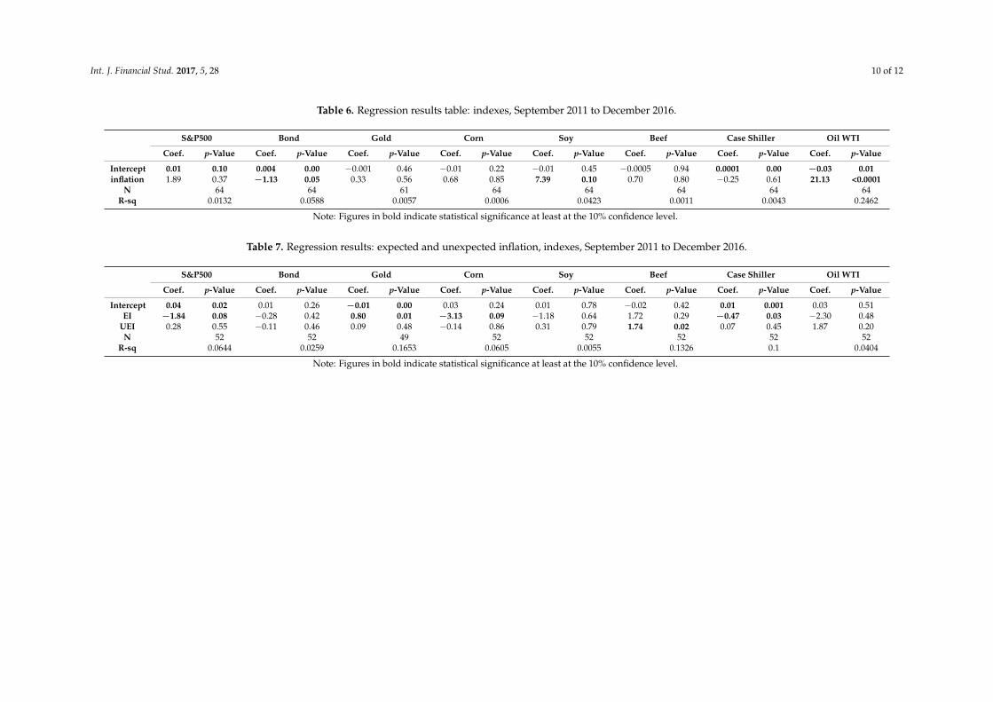
Considering that the data in this study span the period February 1989 to December 2016 forindexes and the period September 2011 to December 2016 for ETFs, it is natural to perform additionaltests to ascertain the robustness of the results. The first test that we perform is based on synchronizingthe data periods, i.e., we perform the same analysis on index but for the shorter, after Great Recessionperiod, which we study for ETFs. These results are presented in Tables 6 and 7.

Table 6 shows that, among the indexes, only bonds, soy and oil have statistically significantregression coefficients. The coefficients for the same time period are significant for bonds, real estateand soy and they have the same sign as the index regression coefficients indicating robustness of results.

Table 7 shows regression results based on Equation (2) when the indexes data period is matchedwith the ETFs data period. These results show that stocks, gold, corn and real estate expected inflationregression coefficients are statistically significant, and beef’s unexpected regression coefficient issignificant. In the ETF sample, only stock ETF expected inflation and beef unexpected regressioncoefficients are statistically significant. A reason for the diffference could be the use of differentunderlying index for the ETF than what we use for the index analysis, since ETFs underlying indexare proprietary. Nevertheless, the signs of the coefficients are the same, which provides proof for therobustness of the results.

Int. J. Financial Stud. 2017, 5, 28 10 of 12

Table 6. Regression results table: indexes, September 2011 to December 2016.

S&P500 Bond Gold Corn Soy Beef Case Shiller Oil WTI

Coef. p-Value Coef. p-Value Coef. p-Value Coef. p-Value Coef. p-Value Coef. p-Value Coef. p-Value Coef. p-Value

Intercept 0.01 0.10 0.004 0.00 −0.001 0.46 −0.01 0.22 −0.01 0.45 −0.0005 0.94 0.0001 0.00 −0.03 0.01inflation 1.89 0.37 −1.13 0.05 0.33 0.56 0.68 0.85 7.39 0.10 0.70 0.80 −0.25 0.61 21.13 <0.0001

N 64 64 61 64 64 64 64 64R-sq 0.0132 0.0588 0.0057 0.0006 0.0423 0.0011 0.0043 0.2462

Note: Figures in bold indicate statistical significance at least at the 10% confidence level.

Table 7. Regression results: expected and unexpected inflation, indexes, September 2011 to December 2016.

S&P500 Bond Gold Corn Soy Beef Case Shiller Oil WTI

Coef. p-Value Coef. p-Value Coef. p-Value Coef. p-Value Coef. p-Value Coef. p-Value Coef. p-Value Coef. p-Value

Intercept 0.04 0.02 0.01 0.26 −0.01 0.00 0.03 0.24 0.01 0.78 −0.02 0.42 0.01 0.001 0.03 0.51EI −1.84 0.08 −0.28 0.42 0.80 0.01 −3.13 0.09 −1.18 0.64 1.72 0.29 −0.47 0.03 −2.30 0.48

UEI 0.28 0.55 −0.11 0.46 0.09 0.48 −0.14 0.86 0.31 0.79 1.74 0.02 0.07 0.45 1.87 0.20N 52 52 49 52 52 52 52 52

R-sq 0.0644 0.0259 0.1653 0.0605 0.0055 0.1326 0.1 0.0404

Note: Figures in bold indicate statistical significance at least at the 10% confidence level.

Int. J. Financial Stud. 2017, 5, 28 11 of 12

6. Conclusions

In this study, we attempt to identify the asset which is the best hedge against inflation. The assetsthat we study are stocks, bonds, commodities, real estate and oil indexes and their correspondingETFs to determine the most beneficial tradable asset in addition to the more theoretical index asset forinflation hedging in the period February 1989 to December 2016 for indexes and September 2011 toDecember 2016 for ETFs.

We find that, out of the eight studied assets, oil is the best hedge against inflation, even thoughthree in total are a good hedge: oil, gold and corn, with corn and oil being complete hedges,and gold being a partial hedge. This is consistent with the findings of Chua and Woodward (1982)and Bampinas and Panagiotidis (2016). Chua and Woodward (1982) find that gold is a goodhedge against inflation, even though in a different time period—January 1975 to January 1980.Bampinas and Panagiotidis (2016) document that energy stocks are a good hedge against inflation.Two have conflicting results depending on whether we examine the index or the ETF—the real estateindex is a hedge, and real estate ETF is the opposite of a hedge. Similarly, the bond index is not relatedto inflation, whereas bond ETF is the opposite of a hedge. We find that stocks, soy and beef are nothedges against inflation.

Acknowledgments: The author would like to acknowlege the support of Nancie Fimbel.

Conflicts of Interest: The author declares no conflict of interest.

References

Alagidede, Paul, and Theodore Panagiotidis. 2010. Can common stocks provide a hedge against inflation?Evidence from African countries. Review of Financial Economics 19: 91–100. [CrossRef]

Alagidede, Paul, and Theodore Panagiotidis. 2012. Stock returns and inflation: Evidence from quantile regressions.Economics Letters 117: 283–86. [CrossRef]

Bampinas, Georgios, and Theodore Panagiotidis. 2015a. Are gold and silver a hedge against inflation? A twocentury perspective. International Review of Financial Analysis 41: 267–76. [CrossRef]

Bampinas, Georgios, and Theodore Panagiotidis. 2015b. On the relationship between oil and gold before andafter financial crisis: Linear, nonlinear and time-varying causality testing. Studies in Nonlinear Dynamics &Econometrics 19: 657–68.

Bampinas, Georgios, and Theodore Panagiotidis. 2016. Hedging inflation with individual US stocks: A long-runportfolio analysis. The North American Journal of Economics and Finance 37: 374–92. [CrossRef]

Baur, Dirk G., and Brian M. Lucey. 2010. Is gold a hedge or a safe haven? An analysis of stocks, bonds and gold.Financial Review 45: 217–29. [CrossRef]

Bodie, Zvi. 1983. Commodity futures as a hedge against inflation. The Journal of Portfolio Management 9: 12–17.[CrossRef]

Chua, Jess, and Richard S. Woodward. 1982. Gold as an inflation hedge: A comparative study of six majorindustrial countries. Journal of Business Finance & Accounting 9: 191–97.

Dempster, Natalie, and Juan Carlos Artigas. 2010. Gold: Inflation hedge and long-term strategic asset. The Journalof Wealth Management 13: 69–75. [CrossRef]

Froot, Kenneth A. 1995. Hedging portfolios with real assets. The Journal of Portfolio Management 21: 60–77.[CrossRef]

Ghosh, Dipak, Eric J. Levin, Peter Macmillan, and Robert E. Wright. 2004. Gold as an inflation hedge? Studies inEconomics and Finance 22: 1–25. [CrossRef]

Int. J. Financial Stud. 2017, 5, 28 12 of 12

Reboredo, Juan C. 2013. Is gold a hedge or safe haven against oil price movements? Resources Policy 38: 130–37.[CrossRef]

Worthington, Andrew C., and Mosayeb Pahlavani. 2007. Gold investment as an inflationary hedge: Cointegrationevidence with allowance for endogenous structural breaks. Applied Financial Economics Letters 3: 259–62.[CrossRef]

© 2017 by the author. Licensee MDPI, Basel, Switzerland. This article is an open accessarticle distributed under the terms and conditions of the Creative Commons Attribution(CC BY) license (http://creativecommons.org/licenses/by/4.0/).