a study of lunar surface radio communication
TRANSCRIPT

national Bureau of Standard
library, H.W.
OCT 8 1964
NBS MONOGRAPH 85
A Study of Lunar Surface
Radio Communication
U.S. DEPARTMENT OF COMMERCE
NATIONAL BUREAU OF STANDARDS
THE NATIONAL BUREAU OF STANDARDS
The National Bureau of Standards is a.principal focal point in the Federal Government for assuring
maximum application of the physical and engineering sciences to the advancement of technology in
industry and commerce. Its responsibilities include development and maintenance of the national stand-
ards of measurement, and the provisions of means for making measurements consistent with those
standards; determination of physical constants and properties of materials; development of methodsfor testing materials, mechanisms, and structures, and making such tests as may be necessary, particu-
larly for government agencies; cooperation in the establishment of standard practices for incorpora-
tion in codes and specifications; advisory service to government agencies on scientific and technical
problems; invention and development of devices to serve special needs of the Government; assistance
to industry, business, and consumers in the development and acceptance of commercial standards andsimplified trade practice recommendations; administration of programs in cooperation with United
States business groups and standards organizations for the development of international standards of
practice; and maintenance of a clearinghouse for the collection and dissemination of scientific, tech-
nical, and engineering information. The scope of the Bureau's activities is suggested in the following
listing of its four Institutes and their organizational units.
Institute for Basic Standards. Electricity. Metrology. Heat. Radiation Physics. Mechanics. Ap-plied Mathematics. Atomic Physics. Physical Chemistry. Laboratory Astrophysics.* Radio Stand-
ards Laboratory: Radio Standards Physics; Radio Standards Engineering.** Office of Standard Ref-
erence Data.
Institute for Materials Research. Analytical Chemistry. Polymers. Metallurgy. Inorganic Mate-
rials. Reactor Radiations. Cryogenics.** Office of Standard Reference Materials.
Central Radio Propagation Laboratory.** Ionosphere Research and Propagation. Troposphereand Space Telecommunications. Radio Systems. Upper Atmosphere and Space Physics.
Institute for Applied Technology. Textiles and Apparel Technology Center. Building Research.
Industrial Equipment. Information Technology. Performance Test Development. Instrumentation.
Transport Systems. Office of Technical Services. Office of Weights and Measures. Office of Engineer-
ing Standards. Office of Industrial Services.
* NBS Group, Joint Institute for Laboratory Astrophysics at the University of Colorado.** Located at Boulder, Colorado.
UNITED STATES DEPARTMENT OF COMMERCE • Luther H. Hodges, Secretary
NATIONAL BUREAU OF STANDARDS • A. V. Astin, Director
A Study of Lunar Surface
Radio Communication
L. E. Vogler
National Bureau of Standards Monograph 85
Issued September 14, 1964
For sale by the Superintendent of Documents. U.S. Government Printing Office
Washington. D.C., 20402 - Price 70 cents

Library of Congress Catalog Card Number: 64-60070

CONTENTS
PAGE
1. INTRODUCTION. 1
2. SYSTEM LOSS 2
3. GROUND WAVE ATTENUATION A 3
4. ANTENNA EFFECTS. 19
5. NOISE EFFECTS 25
6. POSSIBLE IONOSPHERIC EFFECTS. 29
7. CALCULATION OF REQUIRED POWER .................. 36
8. CONCLUSIONS 48
9. ACKNOWLEDGMENTS 48
10. APPENDIX: INPUT IMPEDANCE. ..................... 49
11. REFERENCES 55
12. GRAPHS OF GROUND LOSS 57
13. GRAPHS OF INPUT IMPEDANCE ...................... 87
iii


A STUDY OF LUNAR SURFACE RADIO COMMUNICATION
L. E. Vogler
The problem of point-to-point radio communication on the moon is discussed,and equations and curves are presented to estimate power requirements in lunar com-munication systems. Assuming a smooth surface, consideration is given to groundwave attenuation over both layered and non-layered grounds, antenna ground losses in
situations where ground screens are impractical, noise level estimates in the receiv-ing system, and the effects on propagation of possible lunar ionospheres. An exampleof the calculation of required power for a particular communication system is given,
and further studies are suggested.
1. INTRODUCTION
This monograph presents the results of a study investigating the problem of point-to-point
radio communication on the surface of the moon. It is intended as a survey of all the work accom-
plished in a project sponsored by Jet Propulsion Laboratory and, consequently, much of the material
has appeared in previous papers concerned with various phases of the study [Vogler, 1963a, 1963b;
Vogler and Noble, 1963, 1964] ; the rest of the material, notably the discussions on the effects of
layered grounds and possible lunar ionospheres, has not been published before.
No attempt is made here to analyze in detail one particular type of communication system;
rather, it is hoped that this study may provide part of the general information necessary to the design
of any future lunar surface communication link. For example, the antenna used in a permanently
based installation would most likely be much more elaborate than the one needed for communication
by a mobile exploring party. Once the purpose of the system is determined, the curves herein may
be used to help estimate the frequency, range, and power requirements.
Most of the curves, aside from those figures describing illustrative examples, are plotted in
parametric terms for the simple reason that very little information exists at the present time con-
cerning the exact nature of the lunar environment; however, as more and more data become available,
the curves, using the better estimates of parametric values, will still be useful in the analysis of
communication requirements.
The study is primarily concerned with the propagation aspect of lunar surface communication,
although considerable emphasis has been placed on the evaluation of antenna power losses due to the
proximity of the ground. For low antenna heights and poorly conducting soils, these losses may be
far from negligible, especially where ground screens are impractical. The effects of noise and its
relationship to the desired signal is discussed briefly, consideration being given to galactic and
receiving system component noise.
The lunar model assumed is that of a smooth sphere of radius r = 1738 km. The effects ofo
rough terrain on signal propagation are not included in this analysis, although it is recognized that
such things as knife-edge diffraction, "obstacle gain", etc. , might be important at some locations
on the moon's surface; a study including these mechanisms could be undertaken for particular surface
areas of interest. The present curves are expected to be most useful for applications in the frequency
range from about 1 kc/s to 10 Mc/s. Throughout the present analysis, antenna heights are assumed
to be low enough such that height gain effects are negligible.
1
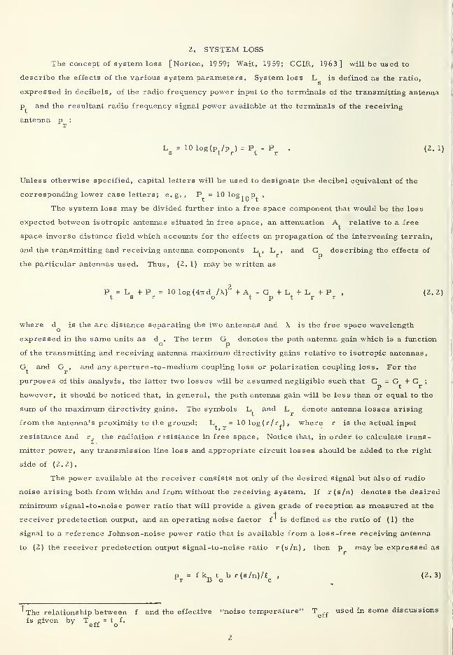
2. SYSTEM LOSS
The concept of system loss [Norton, 1959; Wait, 1959; CCIR, 1963 ] will be used to
describe the effects of the various system parameters. System loss L is defined as the ratio,
expressed in decibels, of the radio frequency power input to the terminals of the transmitting antenna
p and the resultant radio frequency signal power available at the terminals of the receiving
antenna p :
r
Ls
= 10 log(pt/p
r) = P
t- P
r. (2. 1)
Unless otherwise specified, capital letters will be used to designate the decibel equivalent of the
corresponding lower case letters; e.g., P^ = 10 log^p^ ,
The system loss may be divided further into a free space component that would be the loss
expected between isotropic antennas situated in free space, an attenuation relative to a free
space inverse distance field which accounts for the effects on propagation of the intervening terrain,
and the transmitting and receiving antenna components L^, L^, and describing the effects of
the particular antennas used. Thus, (2. 1) may be written as
, 2P = L + P = 10 log (4rrd /X.) + A - G + L + L + P , (2. 2)tsr 6 o t p t r r
x '
where d^ is the arc distance separating the two antennas and \ is the free space wavelength
expressed in the same units as d . The term G denotes the path antenna gain which is a functiono p
°
of the transmitting and receiving antenna maximum directivity gains relative to isotropic antennas,
G and G , and any aperture -to-medium coupling loss or polarization coupling loss. For thet r
purposes of this analysis, the latter two losses will be assumed negligible such that G = G^_ + G ;
however, it should be noticed that, in general, the path antenna gain will be less than or equal to the
sum of the maximum directivity gains. The symbols L and L,^ denote antenna losses arising
from the antenna's proximity to the ground: ^= 10 log(r/r£), where r is the actual input
resistance and r£
the radiation r;sistance in free space. Notice that, in order to calculate trans-
mitter power, any transmission line loss and appropriate circuit losses should be added to the right
side of (2.2).
The power available at the receiver consists not only of the desired signal but also of radio
noise arising both from within and from without the receiving system. If r (s/n) denotes the desired
minimum signal-to-noise power ratio that will provide a given grade of reception as measured at the
receiver predetection output, and an operating noise factor f^ is defined as the ratio of (1) the
signal to a reference Johnson-noise power ratio that is available from a loss-free receiving antenna
to (2) the receiver predetection output signal-to-noise ratio r(s/n), then p may be expressed asr
p = f k t b r(s/n)/4 , (2. 3)r a o c
'The relationship between f and the effective "noise temperature" T used in some discussions
is given by Tg£f
= tQ
f.

where k t b is the reference Johns on -noise power. The symbol k denotes Boltzmann'sB ° -23 Bconstant (= 1.38054 X 10 joules /degree) , t is a reference temperature in degrees Kelvin,
b is the effective noise bandwidth in cycles per second, and is the ratio of the antenna input
resistance to its radiation resistance.
Using the above definitions and assuming i ^ S.^ , (2. 2) may now be expressed as
P. = 32.45 + 20 log d (km) + 20 log f + A - (G + G ) + L, + R + F + B + 10 log (k t ) , (2.4)t o mc t t r t Bo 1 '
where d^ is measured in kilometers, ^mc denotes the radio frequency in megacycles per second,
and R = 10 logr(s/n). The following sections will discuss the various components of (2.4).
3. GROUND WAVE ATTENUATION A
Numerical procedures for the calculation of electromagnetic fields diffracted around a smooth
homogeneous sphere have been developed by various authors [Norton, 1941; Bremmer, 1949 ] .
The ground wave may be expressed as a series of residues that depend on the radius of the sphere
r^, the arc distance d^, the antenna heights h^ and h^ , the free space wavelength X, the
relative dielectric constant e and conductivity cr of the ground, and the polarization of the wave.
As stated in section 1, the present analysis assumes negligible height gain effects corresponding to
antenna heights near zero; for elevated antennas, estimates of height gain may be obtained for beyond
the horizon paths from another paper [Vogler, 1964] .
In parametric form the ground wave attenuation relative to a free space inverse distance field
o,
A^ is conveniently plotted as a function of three parameters : K, b , and x . Through the recent
work of Wait [ 1962 a ] both non-layered and layered grounds may be accounted for by generalizationso
of the definitions of K and b . Thus, with the subscripts h and v referring to horizontal and
vertical polarization respectively,
K, (2.ro/X) 3 |T
h
-1
K :( 2lT ro/M*|T Q (3. 1)
where
\\\ =[<<r -D2+ s
2
], |T
v
2 1,1 1(cr
- 1) + s /(cr
+ s) (3.2)
and
bh
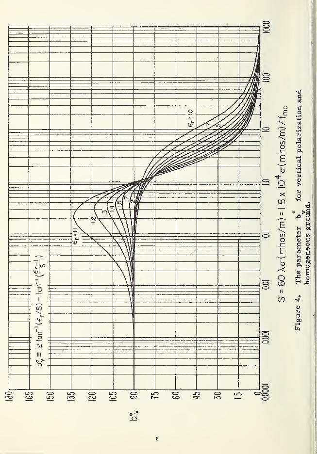
= 180 - tan {—-) - qh ,bv
= 2 tan ( — ) - tanJ
- % (3.3)
with
-7 4s = 2 X 10 c \ cr m 1.8 X 10 cr(mhos/m)/f
3

Both and s are dimensionless and refer to the top ground layer unless otherwise specified.
The parameters X and cr are in meters and mhos per meter respectively, and c is the
velocity of light.
The symbols |Q| and q appearing in (3. 1) and (3, 3) denote the magnitude and phase
of a "stratification factor", Q = |q| exp(iq /2), that accounts for the effect of layering in the
ground. In general Q is a complex quantity dependent on the heights and electromagnetic ground
constants of the various layers, whereas for a homogeneous (non-layered) ground, Q is equal to
unity, Wait [ 1962b ] has derived formulas for Q for the general case of n layers and has pre-
sented curves [Wait, 1962 a] for two and three layer situations; however, unless specific values
for the heights and ground constants of the various layers are given, a graphical representation
becomes quite complicated for a multi-layered ground. For the present discussion, restriction to
vertical polarization over a two-layered model will be assumed.
Letting the subscripts 1 and 2 refer to the upper and lower layers respectively, Q may
be expressed as
i(b° -b° )/2 , i(270°-b° )/2^
T |/|T |)e Vvl V2/+ tanhi(2ttI /\) |
T I ehJ
\ iq°/2
/-
N i(b°-b° )/Z , if 270°- b,° /2. ,, A.
where i is the height of the upper layer measured in the same units as X.|T^
|and | T | are
given by (3.2) using the appropriate values of € and o- characterizing layer 1 or layer 2;„ r
b, and b are obtained from (3. 3) after setting q = 0. As L becomes very large (corre-h v 1
sponding to homogeneous ground), approaches unity and | Q |= 1, q^ = 0 .
Graphs of|T^
jand | T | as functions of and s are shown in figures 1 and 2
where the expressions for refer to a homogeneous ground( |q| = 1); similar plots of b^
o ' o"''
and b^ are given in figures 3 and 4, again for homogeneous ground (q = 0). It can be seen that
b is always positive for either polarization as long as no layering occurs.0
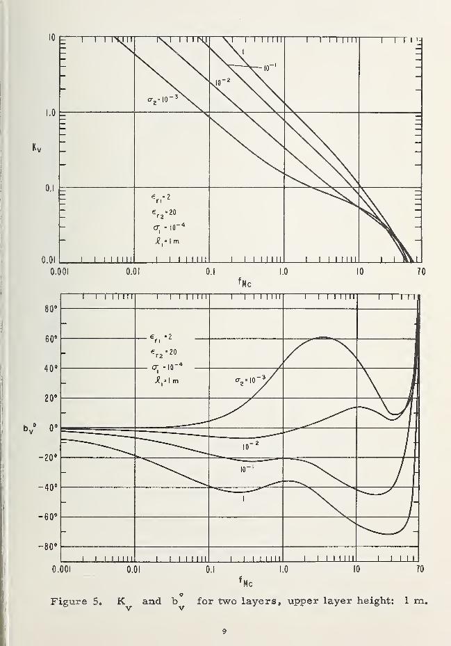
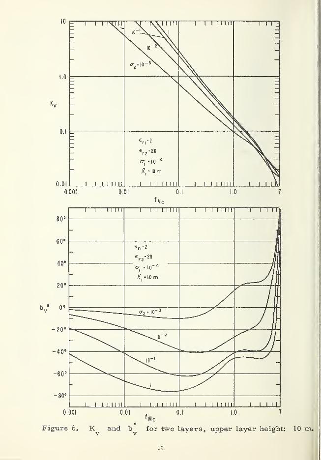
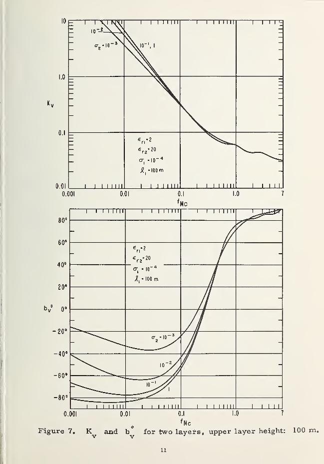
The variation of K and b^ for a two-layered ground is shown in figures 5 through 8 .
The curves were calculated from (3. 1), (3. 3), and (3. 4) using the values of the ground constants
and upper layer heights indicated. Only values of K for 0.01 < K < 10 are plotted since theo
variation of A as a function of b is negligible outside this range (see figures 9 - 14). The curveso o
of b^ indicate that, as the conductivity of the lower layer increases, b is more likely to
become negative. Thus, if it is found that the moon consists of a highly conducting core underlying a
thin poorly conducting crust, ground wave communication could encounter "fade-outs" for certain
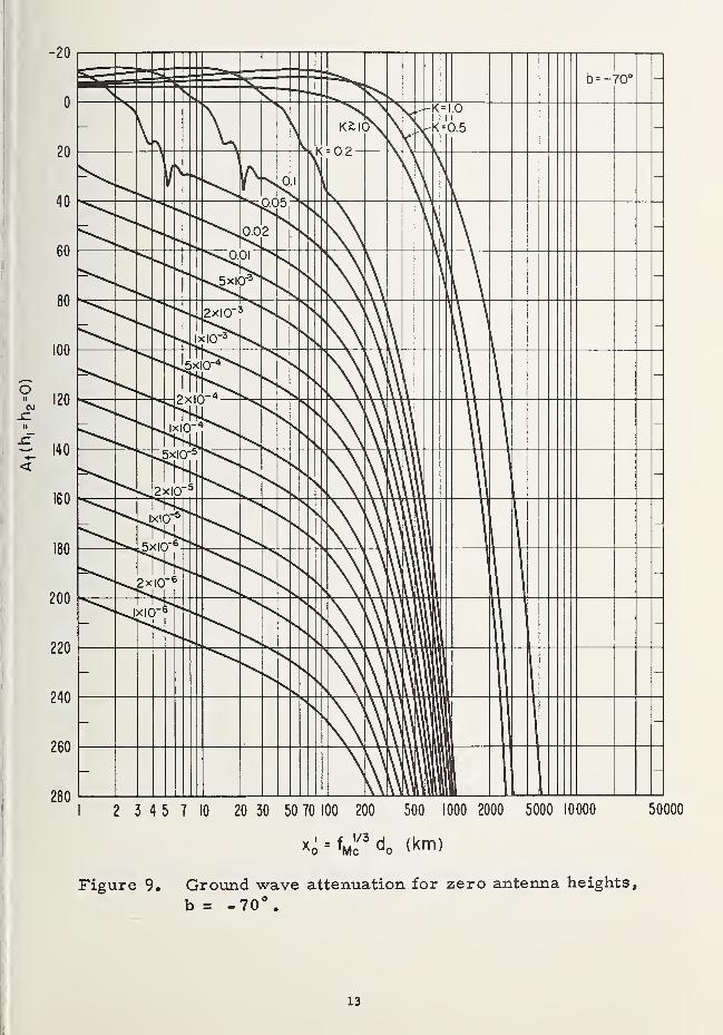
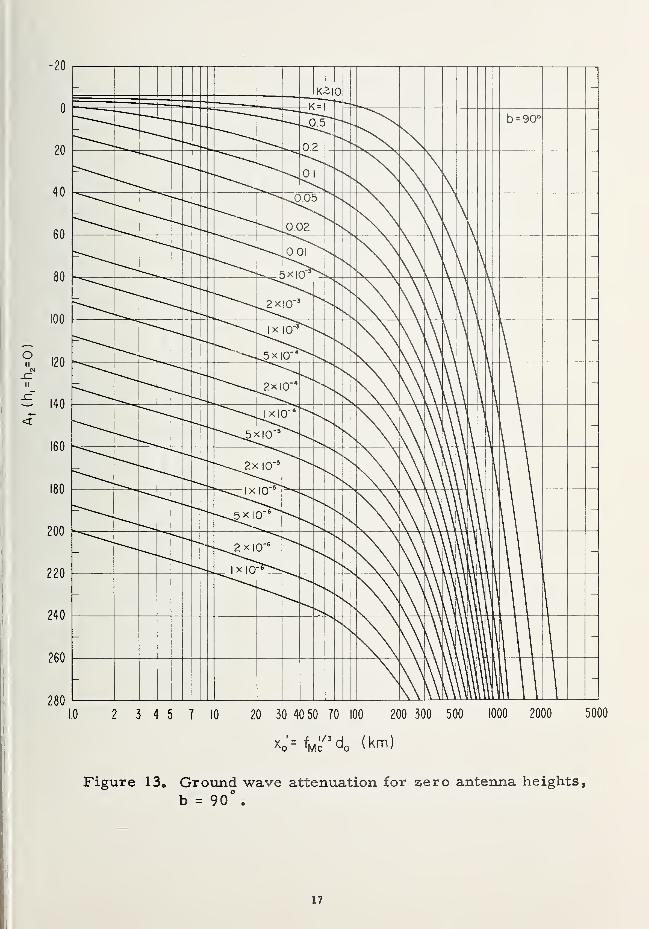
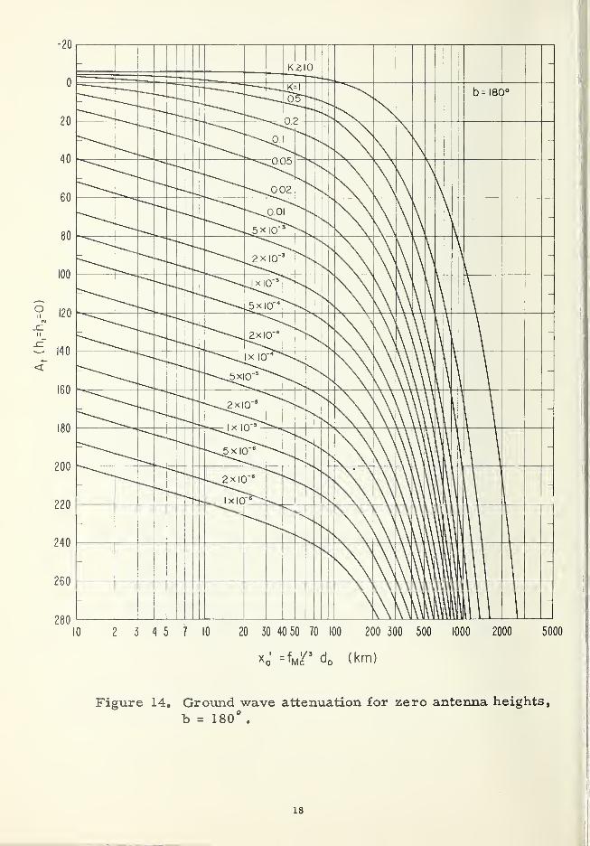
frequencies and ranges. This is indicated in figures 9 through 14 which show the ground wave atten-
uation A^_ for zero antenna heights versus the distance parameter x^ , where
x' = f3 d (km) . (3. 5)
o mc o

5

V(€r-I)
2 + S:
1/2
K v = [(2 IT r0 / X
)
1/31Tv I]
"
'= 3.02 x I0" 2
/ j
T
v |
• fm ,
r0- MOON'S RADIUS = 1738 km
'/3
FOR LARGE S= |TV|~IA/S
0.05 0.1 0.5 1.0 5 10
S = 60Xo-(mhos/m) = i.8x I04 a (mhos/m)/f
50 100
mc
Figure 2. The parameter| T | for vertical polarization. The
formula for assumes a homogeneous ground.
6

7
8

13

1.0 2 3 4 5 7 10 20 30 40 50 70 100 200 300 500 1000 2000 5000
*o'= fMc3d0 (km)
Figure 10. Ground wave attenuation for zero antenna heights,
b = -45° .


5000
Figure 12. Ground wave attenuation for zero antenna heights,
b = 45°.
16
18

In figures 9 (b = -70 ) and 10 (b = -45 ) the curves show fading effects over short intervals of
for certain values of K. As b becomes positive, these fade-outs disappear and is seen
to increase smoothly with distance.
The calculations of the attenuation curves were not done by numerically evaluating the complete
residue series, since a prohibitive number of terms are necessary for small values of x' . In thiso
region (the left hand portion of figures 9 - 14) use was made of the modified flat earth formula
developed by Wait [ 1962 b, see equation (108) ] in which the leading term is the plane earth attenua-
tion function and successive terms account for the curvature of the sphere. The formula with two
curvature correction terms was employed wherever valid until x^ became too large, at which point
the first term of the residue series could be used from there on out.
Equation (2.4) is strictly applicable only for the case of antennas separated a sufficient
distance apart (d^ >> \) such that the induction and static fields may be neglected. Because of
this restriction, A^ is not shown in the figures for values of x 1
< 1 . As d (or x')
goes to
zero, A^ approaches 20 log( 1/2) = -6.02, which would correspond to the surface wave field intensity
expected between short vertical electric dipoles situated near each other on a perfectly conducting
plane.
It is apparent from figures 9-14 that the attenuation is less for the larger values of K,
these values corresponding to vertically polarized waves at the lower frequencies. For example,
for K > 0.1 and f < 1.0, the attenuation is less than 50 db out to distances of 100 km. Onmcthe other hand, with horizontal polarization, is usually much less than unity for all frequencies
and the attenuation is greater.
4. ANTENNA EFFECTS
The terms L, and G = G + G (the subscripts t, r referring to either transmittingt,rptr ° b
or receiving antenna) in (2.2) describe the effects of the particular transmitting and receiving
antennas used in the communication system under consideration. L , called the ground proximityt, r
loss, is defined as the ratio expressed in decibels of the input resistance of the antenna r to its
free space radiation resistance . As the height of the antenna above the surface is increased, the
ratio of the resistances approaches unity and L or L effectively become zero. For heights
near the surface, the input resistance is a function of the electromagnetic ground constants « andr
cr , the radio frequency £c
» an-d the antenna height h above the surface.
G denotes the free space maximum directivity gain of an optimally oriented loss-freet, r
antenna above an isotropic antenna, e. g. , G = G =10 log (3/2) = 1.76 for elementary dipoles and
G = G =2.15 for half-wave dipoles.t r
Because present estimates indicate the conductivity of lunar surface material to be relatively
poor, a numerical evaluation of input impedance was undertaken [Vogler and Noble, 1963, 1964]
considering four types of antennas: vertical and horizontal electric and magnetic dipoles. Short
i oo tdipoles of length di are assumed, the current in which varies as I e with I a constant
o o
along the antenna; the magnetic dipoles are then equivalent to small circular loop antennas of area
dA, the axis being in the direction of the dipole. The ground beneath the antenna is assumed to be
homogeneous and characterized by its relative dielectric constant e and conductivity o- .
19

The input impedance Z, obtained in terms of the field at the antenna, may be divided into a
free space component and a component AZ describing the effect of the presence of the ground:
Z = Z + A Z . (4. 1)
Explicit expressions for the impedance change due to ground normalized by the free space radiation
resistance, AZ/r^, where VED, HE!
of dipoles considered, are then given by
resistance, AZ/r^, where VED, HED, VMD, HMD refer to the initial letters of the four types
VED: AZ/rf= i(3/2 a ) I^N ) + I
2(N
)
HED: AZ/rf
= i(3/4 a3
) fl^l) + I2(N
2)
1
VMD: A Z/rf= i(3/2 a ) ^(1) + I
2(l)
HMD: AZ/rf= i(3/4 a
3) ^(N2
) + I2(l)
, rf
= 20 p2(di)
2,
, rf
= 20 p2(di)
2,
, rf
= 20 p4(dA)
2,
, rf
= 20 (3
4(dA)
2,
(4. 2a)
(4. 2b)
(4.2c)
(4. 2d)
where
Il(
5) = / [
6x2 2 2
x - a (N - 1)
6x +J x - a (N - 1)
> e dx , (4. 3a)
I2(6)
6x -A
2 2,2x - a (N -1
)
> e dx ,
8x + |x2
- «2(N
2- 1)
(4. 3b)
a = 2hp = 2h(2TT/\) ,
2N = € is, s = 60 \ cr(mhos /m) , (4.4)
and h denotes the antenna height in meters above the ground.
The variable x in (4. 3) assumes purely imaginary values from the lower limit to zero, and
from there ranges over real values to the upper limit. The sign of the square root is chosen so that
the real part is greater than zero. A derivation of the dipole impedances together with asymptotic
expressions of (4.2) is contained in the appendix.
Ground proximity loss in terms of the input impedance as given by (4. 1) may be expressed as
L =10 log(r/r ) = 10 log I 1 + Re(AZ/rJ ] , (4. 5)t, r i f
J
20

!where Re(AZ/r ) denotes the real part of (AZ/r ). Using the relationships of (4.2), L, is
1 t t, r
plotted versus
s = 60 \ cr(mhos/m)
-
j
in figures A-l to A-28 for various values of and a. Notice that for a greater than about
5, i.e., h/\ ^, 0.4, the ground loss is always negligible; however, as the antenna height in wave-
lengths approaches zero, L may become quite large for certain combinations of ground con-t» r
ductivity and frequency. It is often possible to reduce the effect of the ground through the use of
appropriate ground screens. Discussions of this subject are contained in papers by Wait and
Surtees [ 1954 ] and by Wait [ 1956 ]
.
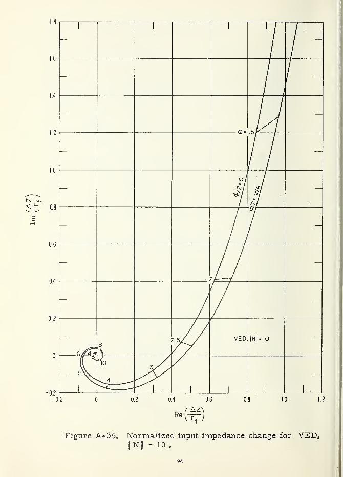
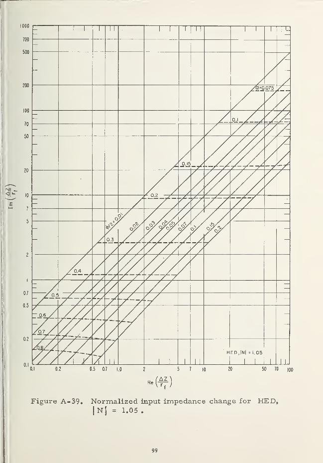
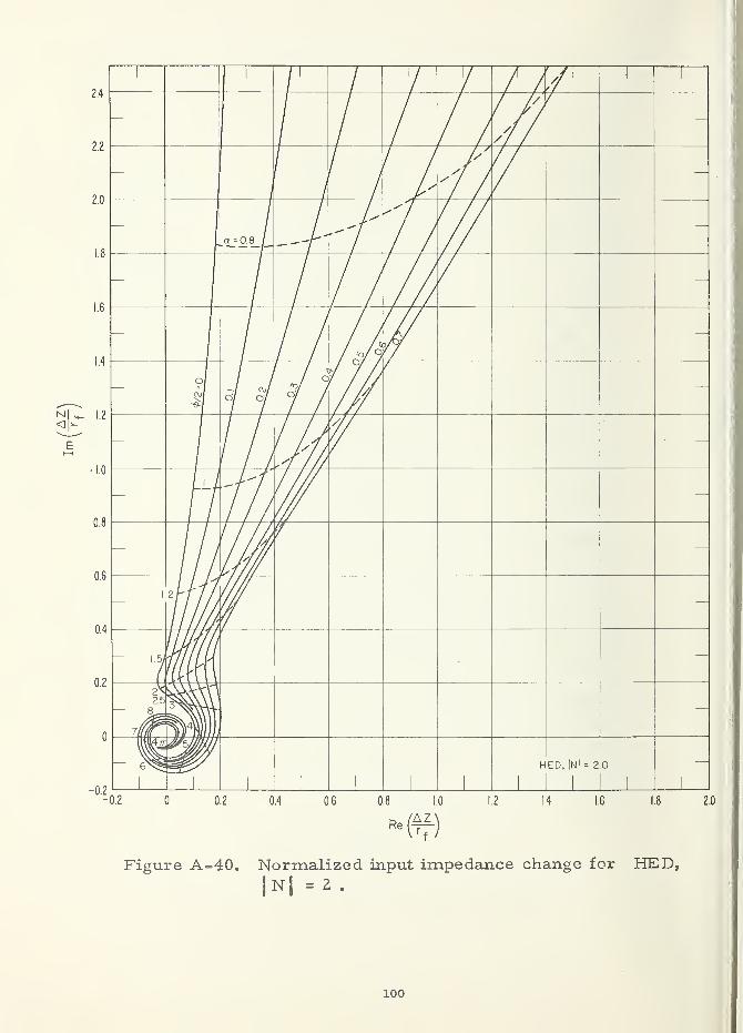
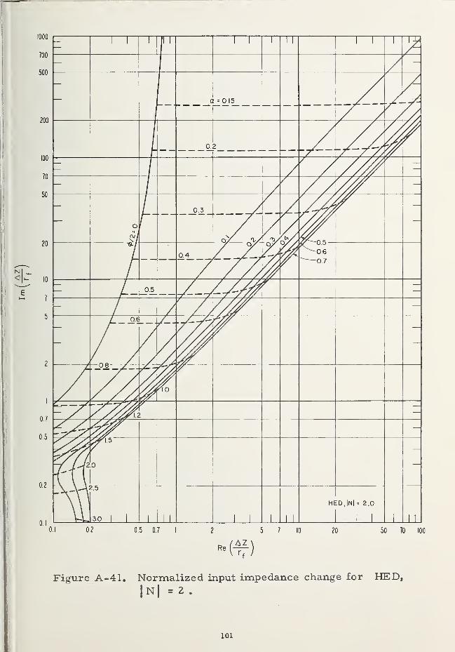
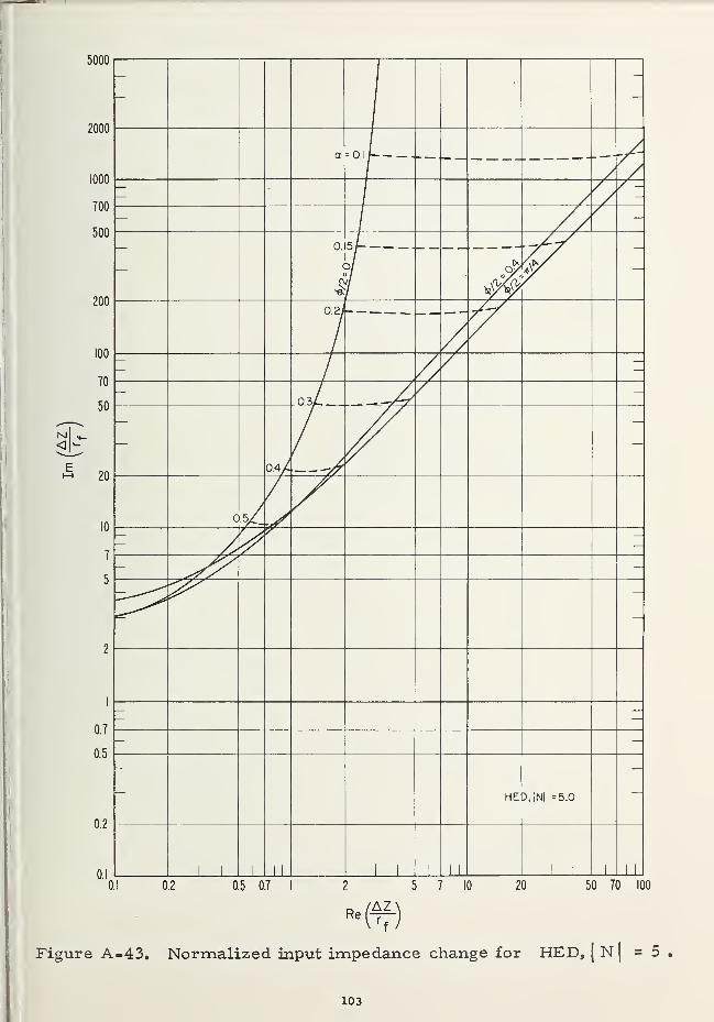
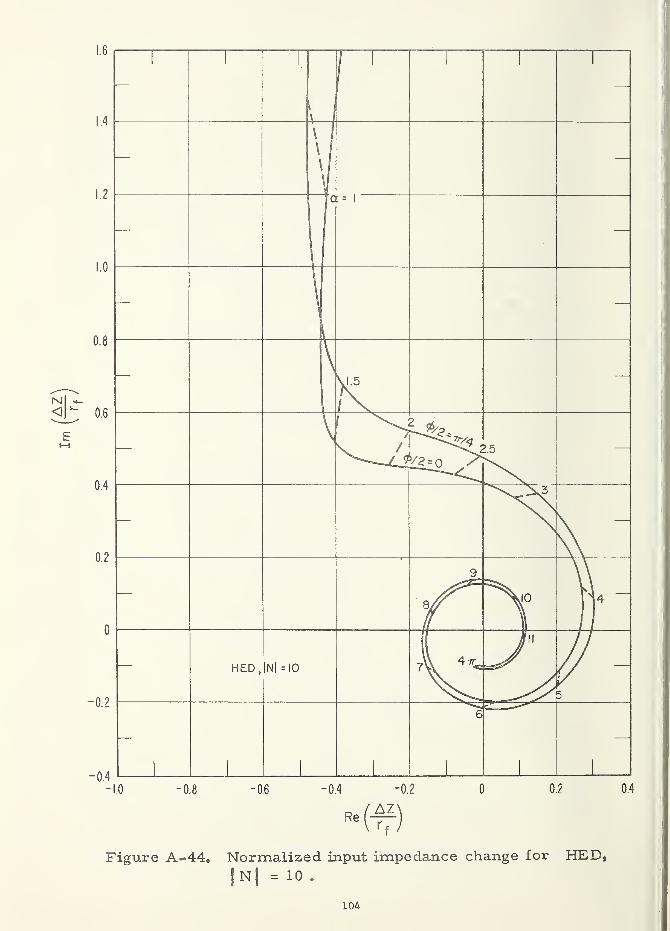
To show the variation in the normalized input impedance change for both the resistance
(Re AZ/r^) and the reactance (ImAZ/r^), equations (4.2) are evaluated and plotted in figures
A-29 to A-64 as functions of |n| , (j>/2, and a where,
/ 2 2\X/
* 1
lN
l= («
r+ s ) ' +/2 = (Vi) tan" (B/
<r) , (4.6)
with a and s as defined in (4. 4). It should be emphasized that figures A-29 to A-64 do not
show the total input impedance, but only the variation due to the presence of the ground. Impedance
curves such as those in the figures are useful not only in estimating antenna requirements for lunar
communication systems, but also may be used in determining the electromagnetic characteristics of
material composing the moon.
This section will conclude with a brief discussion of the Beverage wave antenna [Beverage,
Rice, and Kellogg, 1923 ], If considered for semi-permanent installations on the moon, it has the
advantage of relatively simply construction and operates most efficiently over poorly conducting soils.
The wave antenna in its simplest form consists of a long horizontal wire situated a short height above
the ground and terminated at one end through its characteristic impedance. It is a uni-directional
antenna with the maximum gain in the direction of the antenna axis and toward the terminated end.
Wait [1954] has shown that the vertical electric field component of a wave antenna is pro-
portional to a complex factor T , termed the "wave tilt" and defined by
Tv
(fr
- 1) - is] /(«r - is> . < 4 - 7
)
and a function S' which depends on the wavelength \, antenna length i, an angle<|>
measuring
the direction in which the antenna is pointing, and the propagation constant T defined as
r = a' + i(3m , (4. 8)
where a' and m are real and (3 = 2tt/X.
2 1
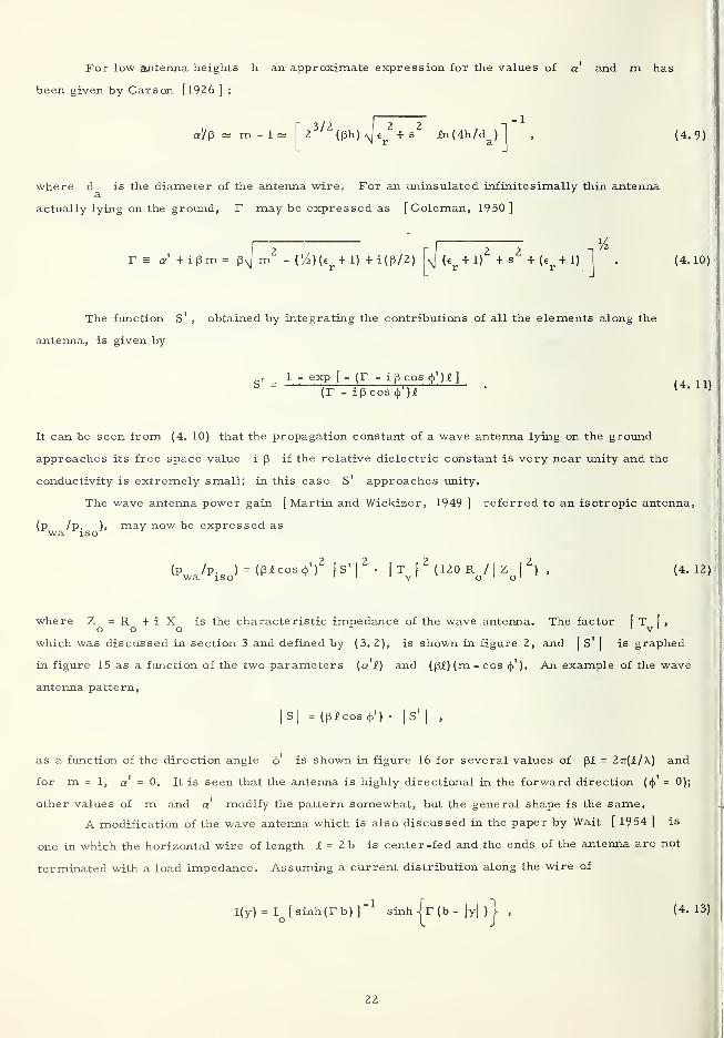
For low antenna heights h an approximate expression for the values of a' and m has
been given by Carson [1926 ] :
df'/p =a m - 1 23/2
(ph) N]er
2+ s
2£n(4h/d
a ) (4.9)
where d is the diameter of the antenna wire. For an uninsulated infinite simally thin antennaa
actually lying on the ground, T may be expressed as [Coleman, 1950 ]
r is a + i pm = PnJ m2
- + 1) + i(P/2) (€r+ l)
2+s
2+(€
r+ l) (4.10)
The function S' , obtained by integrating the contributions of all the elements along the
antenna, is given by
, _ 1 - exp [- (r - ipcos 4>')l]s " (r - ipcos^')£ •
(4<11)
It can be seen from (4. 10) that the propagation constant of a wave antenna lying on the ground
approaches its free space value i p if the relative dielectric constant is very near unity and the
conductivity is extremely small; in this case S' approaches unity.
The wave antenna power gain [Martin and Wickizer, 1949 ] referred to an isotropic antenna,
(p /p. ), may now be expressed aswa iso
(Pwa /piso )
= (|3iCOS *' )2l
S '|2
* ^vl2
^lZQK
ol
\
Zo\
2'
)'
(4 ' 12)
where Z = R + i X is the characteristic impedance of the wave antenna. The factor I T I ,
o o o 1 v 1
which was discussed in section 3 and defined by (3. 2), is shown in figure 2, and I S1
| is graphed
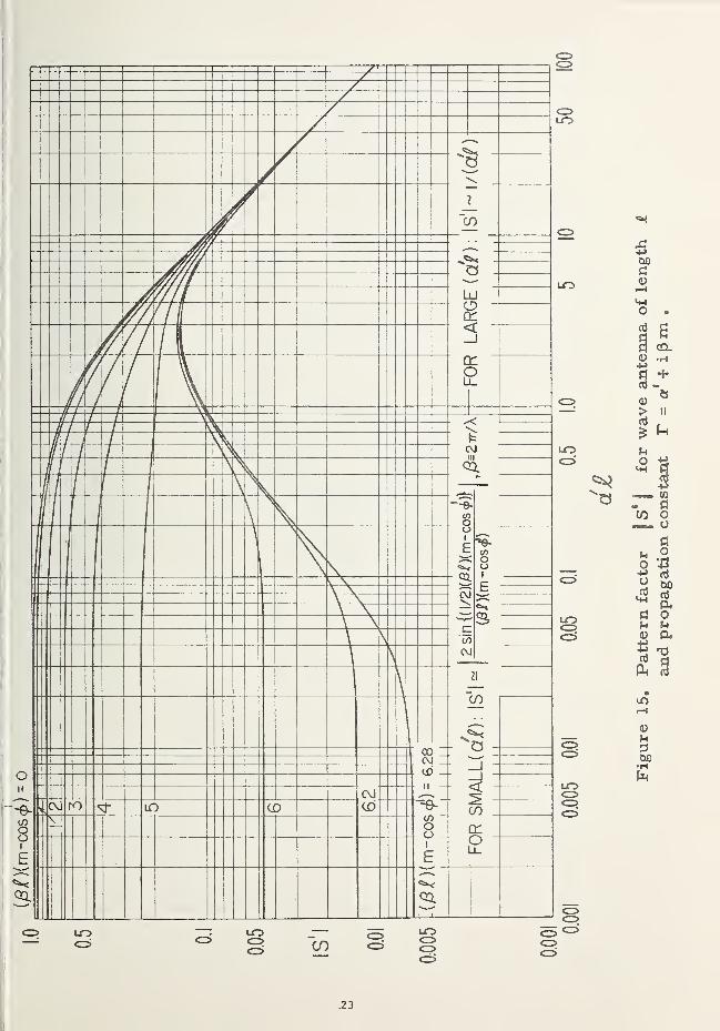
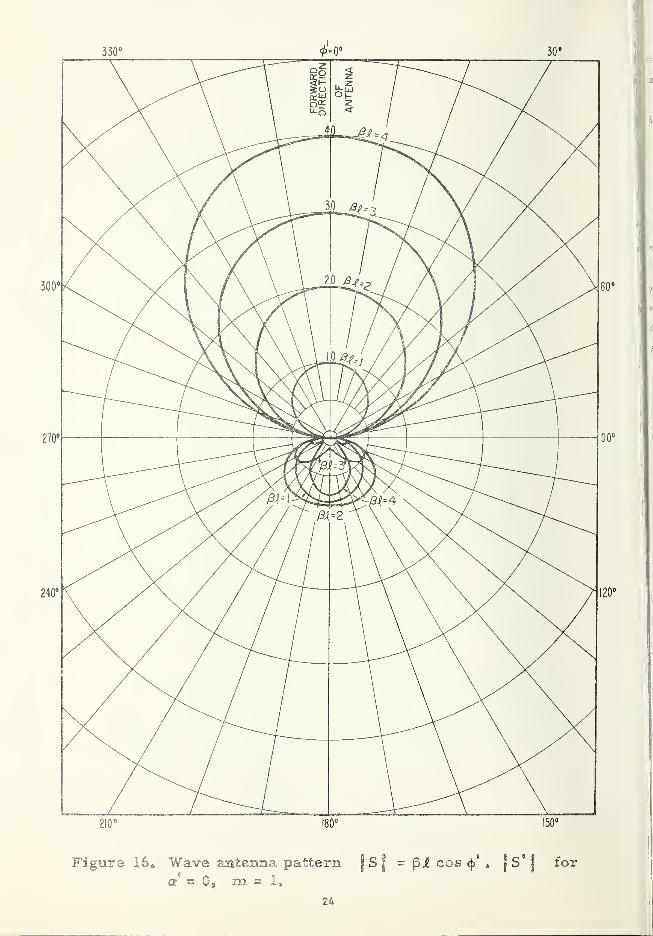
in figure 15 as a function of the two parameters (a'l) and (pj?)(m-cos 4>'). An example of the wave
antenna pattern,
|S
|
= (picos <j>') •| S'
| ,
as a function of the direction angle tj>' is shown in figure 16 for several values of pi = 2tt(£/\) and
for m = 1, a' - 0. It is seen that the antenna is highly directional in the forward direction (cj)' = 0);
other values of m and a' modify the pattern somewhat, but the general shape is the same.
A modification of the wave antenna which is also discussed in the paper by Wait [ 1954 ]is
one in which the horizontal wire of length L = 2b is center-fed and the ends of the antenna are not
terminated with a load impedance. Assuming a current distribution along the wire of
I(y) = I [sinh(rb)]
_1sinh Jr(b- |y| ) i ,
(4.13)
22
.23
where I and y are respectively the current at and the distance from the feed point, an integra-
tion of the elements over the length of the antenna yields for the antenna pattern|S
j:
Ipbcos 4>'|
• \S±\
r
2i cosh x - cos (x 0 -x,I 1 2 :
x, +(x2-x
3 y
'.\ cosh x^- cos (x2+x
3)
xi
+^x2+ x
:
2 2x + x1 2
cosh x - cos x2
(4. 14)
where x„ or b, x^ = (3b m , and x^ = |3b cos <j>
Graphs of (4= 14) are shown in figure 17 for the case of a = 0, which corresponds to very
poorly conducting ground. The values of| S |
shown on the figure, however, should be used only
with antenna lengths I such that the quantity {a I) is very near zero; if this is not the case,|S
|
should be calculated from (4. 14), The center-fed wave antenna power gain corresponding to (4. 12)
is given by
P /p.wa iso|S|
2-
|T
I
2( 120R / |
Z |
2(4.15)
where T | , R and Z have been defined previously,o
The theoretical determination of L or L for a wave antenna in terms of its inputt r
resistance is quite difficult. However, considering these quantities essentially as power ratios
measuring the effectiveness of the antenna, an estimate of their magnitude may be obtained from
(4. 12) by assuming that
L - Gt, r t, r
10 log (p /p.v wa iso
(4. 16)
5. NOISE EFFECTS
The operating noise factor f [Norton, 1962 ]appearing in (2.4) provides a measure of
the effects of noise on the receiving system (in previous papers [Vogler, 1963a, 1963b] f is
called the effective noise figure). It is defined by
f =[Pa/% tQb)]/[r(s/n)] , (5.1)
where p_^ is the signal power available from an equivalent loss -free receiving antenna, (k^ t^ b)
is a reference Johnson-noise power [see (2.3)], and r(s/n) is the receiver predetection output
signal-to-noise ratio.
Since p is the power available from a loss -free antenna, its relationship to the powera
available from the actual antenna, p , may be expressed asr
p = I p , (5.2)a c r
25

26

where jf is the antenna circuit loss factor. Because the present study is primarily concerned with
low antennas over poorly conducting ground, the assumption is made throughout that £ I ,
c r
where I is the ground proximity loss discussed in section 4.
In terms of the noise factors of the receiving system's component parts, f can be expressed
in the following form:
f = f - l+ f + £ (f _ 1) + £ £ (f _ 1)e c c
xti ' ctTr '
' (5. 3)
where f^, f^, f , and denote respectively the noise factors of the external noise, antenna
circuit, transmission line, and receiver. In terms of the loss factors £ and £ of the antennac t£
circuit and transmission line (i. e. , the ratio of the available input to output powers of the component),
f^ and f^ are given by
fc=l + (*
c-l)(t
c/to ), V= 1+^-1) (tu /t
o) , (5.4)
where t^ and t^ designate the absolute temperatures of the corresponding components and t is
a reference temperature.
Generally speaking, the factors f and f will predominate in calculating values of f,
especially at the lower frequencies [Crichlow, Smith, Morton, and Corliss, 1955 ]; at high fre-
quencies f depends more on f and f , which are best obtained by direct measurement. By
arbitrarily assuming the transmission line loss to be negligible (i = 1) and the antenna circuit
temperature very near the reference temperature, ( 5. 1 )may be written as
f-= f +1 f - 1 , i = 1 , t = t . (5. 5)e c r t£ co
With the approximation £ ^ i , this then becomesc r
f .as f + i f - 1 , (5. 6)errwhere £ has been defined in section 4.
r
The principal sources of external noise received by an antenna located on the moon are
(1) galactic or cosmic, (2) earth-based, and (3) solar. The amount of noise affecting the signal
depends on the location, orientation, and directional gain of the particular antenna under considera-
tion. Some preliminary studies [Page, 1962 ] of earth-based and solar noise components indicate
that, in the case of a quiescent sun, solar noise is negligible compared with galactic noise unless
the antenna beam is oriented directly toward the sun. On the other hand terrestrial atmospheric
noise might become comparable to the galactic noise in the lower frequency range; however, this
assumes a negligible ionospheric shielding effect.
Galactic noise levels have been fairly well established at the higher frequencies through
earth-based measurements. Figure 18 shows an estimate of the external noise factor = lOlog f
obtained from galactic noise data compiled by Menzel [ 1961 ] and by Hartz [ 1963 ]; the reference
27

UJ
i
Nl
Z Jj /£ /
/ 0
Co
9
// <J
/
//
//
y/
/
1
—j-
/A/ h-—/ <r—7— / <
/ T
-h-fj
1
/ -1—T11
i
/—/
—
1
1i—f——f—
/
/
—
/ i—/
/1
/—t
i
/ i/
//
/
i
/
/
9j 601 01 = 8d
28

temperature assumed here is tQ
= 288. 37 K. Empirical expressions used to plot the galactic noise
curve are
f = 6.467 X 10 f , f > 200 ,
e mc mc
(5.7a)
f = 1.585 X 10⁵
f~ Z ' 3
, 10 < f < 200,e mc mc
from the Menzel data, and
f = 5.012 X 10⁴
£" 1 ° 8
, 0.5 < £ < 10 , (5.7b)e mc mc
from the Hartz data obtained from Topside Sounder measurements. The upper and lower dashed lines
-2 3 -18on the figure are extrapolations of the f " and f ° frequency variations.mc mc
It is physically apparent that at some lower frequency the galactic noise curve will at least
level off. Until information from low frequency measurements are available, the extrapolations of
figure 18 maybe used to provide (hopefully pessimistic) estimates of galactic noise.
6. POSSIBLE IONOSPHERIC EFFECTS
At the present time there is no indication that the moon possesses a neutral atmosphere of
any significant magnitude. Because of this, it is unlikely that lunar surface propagation will be
affected by ionospheric considerations to the same extent as terrestrial propagation. However,
studies have been made showing the possible existence of a weak lunar ionosphere caused by solar
wind. This section will discuss briefly the effect on propagation of two forms of possible ionospheres.
If a negligible magnetic field is assumed and the motion of heavy ions is neglected, the
ionosphere may be characterized by its index of refraction N. as follows :
(6.1)
where f denotes the signal frequency, f the collision frequency, and f the critical ormc b ^ ' v cr
plasma frequency, all measured in Mc/s. In terms of the electron density/cm , n, the critical
frequency is given by
f2
8.1 X 10" 5n, (6.2)
cr
where, in general, n is a function of the height h above the ground: n = n(h)„
One form of ionosphere that may possibly occur extends from the moon's surface to some
distance above, the electron density decreasing with height. Elsmore [ 1957 ] , using studies of
lunar occultation of the Crab Nebula, has hypothesized surface electron densities on the order of
3 4 310 to 10 electrons/cm . For signal frequencies near or less than the collision frequency, this
ionospheric model presents a propagation problem which, as far as the author is aware, has never
29
been investigated and is beyond the scope of the present paper. Considerable theoretical study
would be necessary to determine propagation characteristics at these low frequencies.
For radio frequencies such that f /f < < 1, an estimate of the effect of a surface ion-v mc
osphere on propagation at frequencies greater than the plasma frequency may be obtained through
the concept of effective radius [Burrows and Atwood, 1949 ]. The effective radius, r , intro-
duces a correction to the actual radius, r , that allows for the refraction of the radio wave as ito
travels through the medium (in this case the model ionosphere) above the ground. Expressed in
terms of an effective radius factor k [Wait, 1961 ] :
r
k= —ro
1 +
r N. (h=0)o 1
N (h=0)(6.3)
where N. (h=0) denotes the gradient of the refractive index with respect to height evaluated at the
surface.
With the restriction that f /f < < 1, (6. 1) may be rewritten asv mc
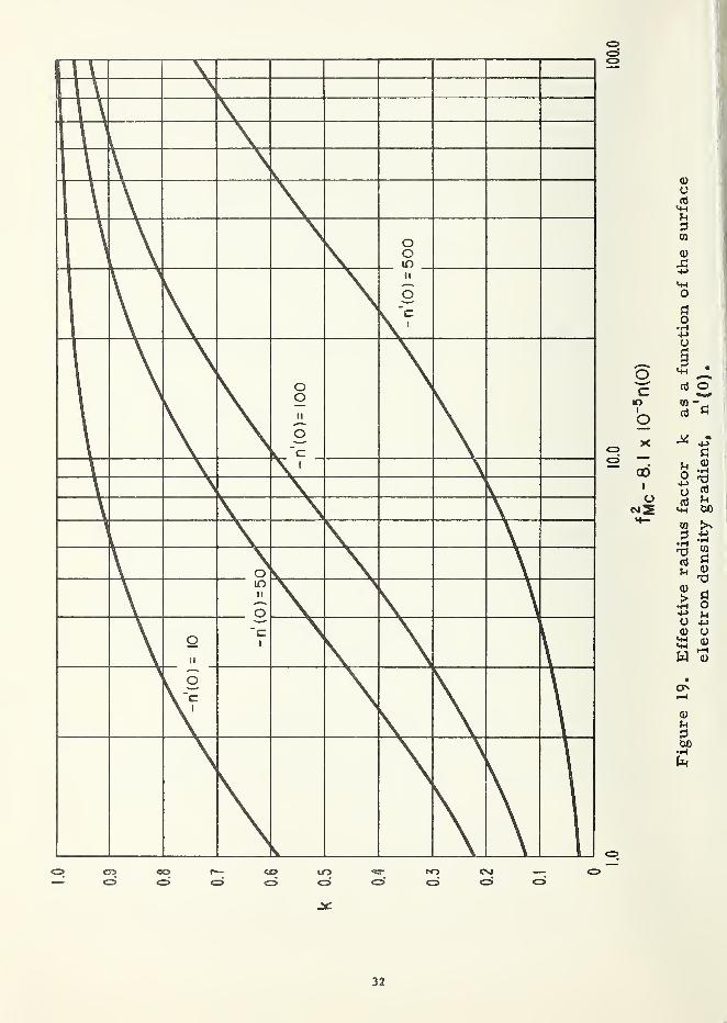
2 2,2 -5,2NNl-f /f = 1 - 8.1 X 10 n(h)/fl cr mc mc (6.4)
and k then becomes
k -a 1 +
4.05XlO"5r {-n'(0)}o
2 2N. (0) f
l mc
1 +
0.07 { -n' (0) }
- 8. IX 10_5
n(0)
(6.5)
where n(0) is the electron density/cm at the surface and n (0) is the electron density gradient
with respect to height in km evaluated at the surface. It can be seen that (6. 5) may be used only
for radio frequencies such that
-3f > f = 9 X 10""
\l n(0)mc cr
thus, for an electron density at the surface of, say, n(0) =10 , the effective radius concept should
be restricted to frequencies of 1 Mc/s or greater.
The curves of figures 9-14 will now provide estimates of the attenuation if they are
read as functions of a modified x' , x'(k), and a modified K, , K, (k) , whereo o h, v h, v
i A ? - -(k) = k" 3
f3 d (km) , K(k) = 3.02 X 10" k~ 3/| T I
•I Q I
• f3
,mc o TT, <~(6.6)
and k is given by (6.5). Notice that x (1) and K(l) are simply those parameters discussed l-n
section 3 and defined by (3. 5) and (3. 1); the effective radius factor k does not modify bh, v
30

To show the variation of k with frequency, (6. 5) is plotted in figure 19 for several values
of the surface electron density gradient n'(0). The values chosen do not. represent any experimental
evidence but are used merely to show the variation of k with the gradient. Figure 19 shows that,
as the gradient becomes more negative, k decreases and, in general, a higher attenuation of the
signal is to be expected. Should a positive gradient exist, less attenuation of the signal would occur.
Another possible lunar ionosphere that has recently been investigated [Weil and Barasch,
1963 ] is similar in form to the terrestrial ionosphere. Weil and Barasch, through theoretical
considerations of solar wind influence near the moon together with solar stream data, postulate an3
ionized elevated layer with an electron density of about 350/cm at 0.6 lunar radii above the
surface. The layer occurs only in the general direction of the sun, and their numerical values are
based on quiet sun data.
The theory of this form of ionospheric propagation is well established and, given the neces-
sary data, will provide good estimates of propagation capabilities. The remainder of the section
will discuss briefly the simple geometrical-optics approximation to ionospheric propagation. A
detailed account of the subject is contained in a paper by Wait [ 1962 c ] .
In the geometrical-optics approximation, the field at a point is considered to be the sum of
multiply-reflected radio rays arriving from the transmitting source, the reflections occurring
between the ground surface and the ionosphere. At distances less than its caustic, the single hop
component of the field, i. e. , the ray undergoing only one reflection from the ionosphere, will be
the most significant. However, the total field is given by the sum of all the rays added together in
proper phase; at short distances from the transmitting antenna, the ground wave component must
also be included.
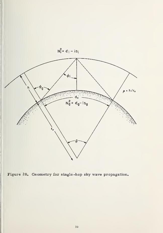
In order to gain some idea of the effect on lunar propagation of an elevated ionosphere, the
attenuation of the single -hop sky wave is evaluated, assuming the Weil and Barasch model iono-
sphere with a sharp lower boundary. The assumption of a sharp boundary rather than a more
realistic one will give a lower estimate of the attenuation than is actually obtainable, but will still
provide a reasonable estimate for the purposes of the present study. Letting 6( = d^/r^) ,
p( = h/r^), cj>^, and <j>^ denote the geometrical quantities indicated in figure 20, the sky wave
attenuation Ag
may be expressed as
A ~ - 20 lofs
e
C sin2 4> \2
(6.7)
where R and R. are Fresnel reflection coefficients of the ground and ionosphere respectively :
S i
N 2 cos (j> -J N 2 - sin2
2 | I 2cos (j>^ +^ N - sin 4>^
-, N2
= e -is , (6.8)
31
ooin
ow "cX 1
r n'(0)=
100
i\ 1
omii
o
oII
"ci
i
c
00I
o
COd
32
N?= €j- iSi
33

2 2 2N. cos <j>. -
\JN. - sin <j>.
R.1
2 2 2cos <j). + N. - sin (j>.
, N. = e. - i s. ,li l(6.9
and the angles ejj and tj>. may be calculated from
<i> = tan-1 (1+p) sin(9/2)
(1+p) cos (9/2) - 1 I
' vi
-1sin tb
J1+p
(6. 1
The quantity C in (6. 7) is a convergence coefficient defined by
1 + Pcos (9/2)
1 +sin (9/2)
(1+p) cos (9/2) - 1(6. 1
and 9j
is related to the total distance traversed by the ray:
Ij =\J p
2+ 4(1 +p) sin
2(9/4) (6. i;
Notice that (6. 11) [and therefore (6. 7) ] is valid only as long as
< 9c
= 2 cos"1
[ l/(l + p) ]
9 corresponds to the distance at which a caustic is encountered, and other formulas must be usedc
to calculate the attenuation in this region. The distances considered here will be only those such
that 9 < < 9 .
c
At VLF and for the distances of interest, the reflection coefficient of the ground R is nearg
unity even for the very poorly conducting ground expected on the moon. On the other hand, the ion-
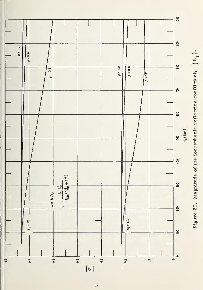
ospheric reflection coefficient R^ can have a pronounced effect on propagation estimates. Figure
21 shows a plot of|R^
|as a function of the ionosphere height p= h/r^ and
s. = f f2/f (f
2+ f
2
l v cr mc \ mc v
obtained from (6. 1). Notice that| R.
|depends quite critically on the parameter and, hence,
on estimates of n and f . If an elevated lunar ionosphere does exist, data concerning these quan-
tities are necessary for VLF propagation predictions. The purely geometric factor ,
.1
»
34
IN- CO lO rO CM
35

C sin2
*g )y/(
2 91/ e )
appearing in (6.7) depends only on the distance d between the transmitting and receiving points
and on the height of the ionosphere; curves of this factor are presented in figure 22 for various
values of p .
The attenuation Ag
of a single -hop sky wave relative to a free space inverse distance field
is shown in figure 23 as calculated from (6.7). For these curves the ground is described by2 .2
N = 2 - i 180, and the ionosphere at a height p = 0.6 is described by N. = 1 - i s. , where sg 'ill
assumes the values 1 and 10. At a radio frequency of f = 0.01, for example, the curvesmcwould be valid for a ground conductivity o- = 10 mhos/m and an ionosphere described by two
values of the ratio (n/f ) 125 and (n/f ) 1250 ; the latter values assume f >> f . Thev v v mc
dashed curves hi the figure show the vertically polarized ground wave attenuation for
f = 0.01 and 0.1; this component of the field is dominant at the shorter distances. It can bemcseen that over the range of distance shown, the difference in attenuation between the two sky wave
curves is about 10 db, this difference arising from the ionospheric reflection coefficient FL.
A change in ground constants at VLF produces very little difference in attenuation for a given s.„
According to Weil and Barasch [ 1963 ] the ionosphere would exist (with any appreciable
magnitude) only within about 60 from the sun-moon line; thus, it would not be a dependable
mechanism for long-term propagation. It should be remembered, however, that it could occasion
interference effects in VLF ground wave communication circuits at those distances where the ground
wave and sky wave components are comparable in magnitude.
7. CALCULATION OF REQUIRED POWER
Attempts have been made recently to deduce the electromagnetic properties of the moon's
surface material through the use of radar data [Senior and Siegel, I960 ]. Although differences
exist concerning the exact interpretation of the data [Brown, I960; Daniels, 1961 ], there is
general agreement that the relative permittivity is not far above unity and that the conductivity is
quite low. In any cate, most of the graphs discussed in the preceding sections are applicable to a
wide range of values of 6 and u .
r
Senior and Siegel estimate the relative dielectric constant and conductivity of lunar surface_4
material to be e = 1. 1 and cr = 3.4 X 10 mhos/m. Materials constituting the earth's crustr
have been found with conductivities of this order, but not with such a low permittivity. For the
purpose of arriving at some estimate of lunar propagation conditions, it will be assumed that e
-3 -4r
ranges from 1.1 to 2.0 and o- lies between 10 and 10 mhos/m.o
By choosing a reference temperature t = 288. 37 K (as in section 5), the required power
given by (2. 4) may be rewritten as
P=L -(G+G) + L+R + F+ B- 204 (7. 1)t p t r t
where the propagation loss L^ for ground wave attenuation between isotropic antennas is given by
36

37

38

L = 32.45 + 20 log d (km) + 20 log f + Ap o mc t
(7.2)
For sky wave propagation, would be calculated by (7.2) after replacing by the A dis-
cussed in section 6.
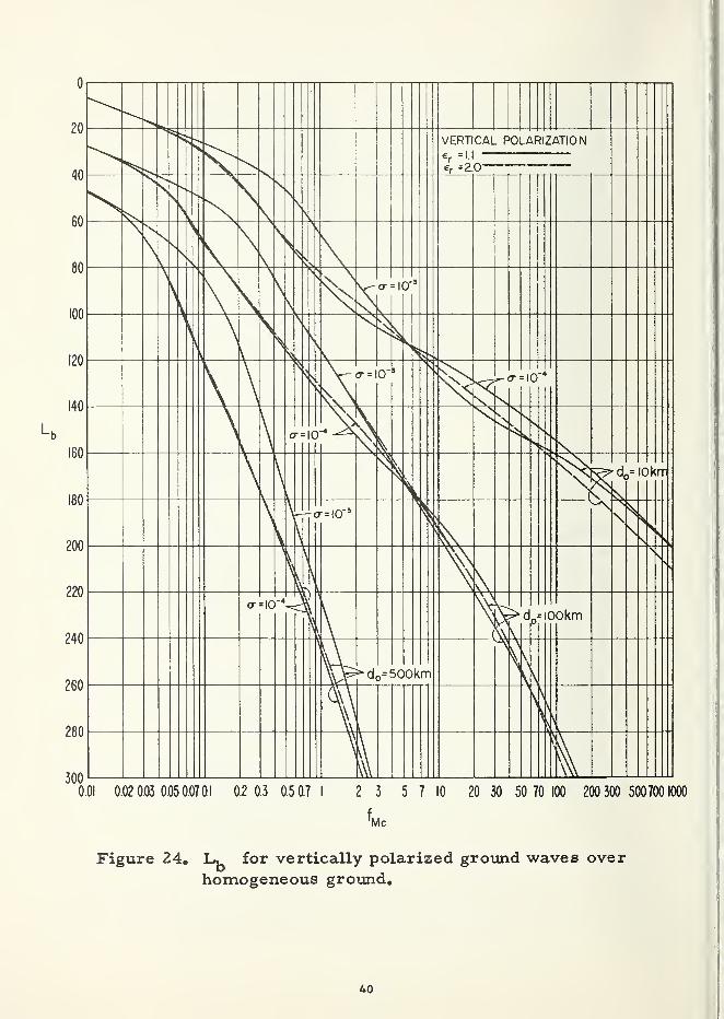
Figure 24 shows curves of for a vertically polarized ground wave over homogeneous
ground as a function of frequency and distance. Values of A^ were obtained from figures 11o
through 14 by linear interpolation in both the and b^ directions, being given by figure 2
and (3. 1) with I Q I = 1, and b being read from figure 4. Notice that L, varies inverselyv 1 v
f./' p
with conductivity at the lower frequencies, while at high frequencies the effect of cr variation
becomes negligible.
To show the use of (7. 1) in estimating required power for a particular communication
system, the following example will be considered. Assume a communication system consisting of
a wave antenna lying on the moon's surface and transmitting towards a short vertical electric dipole
i0
placed some distance away and in an optimum direction from the transmitter (cj) ~ 0 ). An estimate
of - may be obtained from (4. 16) and (4. 12) by assuming the free space value for the
wave antenna characteristic impedance:
I Z I R ~ 120 tt .1 o 1 o
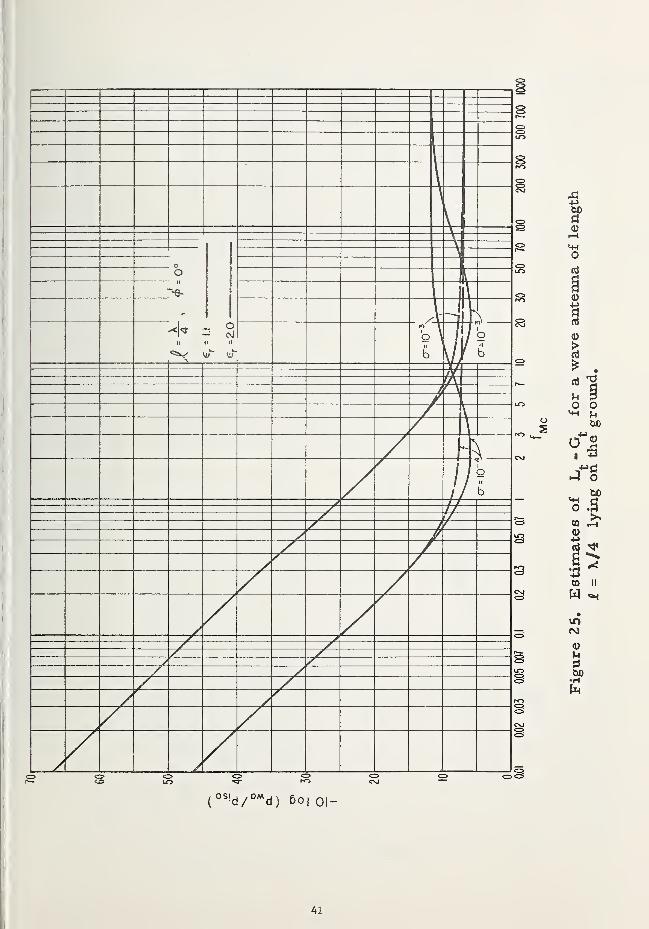
For the case of an antenna of length I - X./4, - is plotted versus frequency in figure 2 5.
Again, the antenna loss varies noticeably with conductivity at the lower frequencies, but not at the
higher ones.
A comparison of figure 18 and figures A-l and A-2 shows that for a dipole at a height of,
say, h = X/16 the external noise tends to "blanket out" the effect of the antenna circuit loss. This
is shown in figure 26, which is a plot of the operating noise factor as given by (5. 6) with an assumed
receiver noise factor of f = 4. Now by using figures 24, 25, and 26, and the dipole gain of
G = 1.76, the required power delivered to the transmitting antenna terminals for a given type of
service may be estimated from (7. 1). Figure 27 shows values of P - (R+B) as a function of
frequency for antenna separation distances of 10, 100, and 500 km.
To estimate the required power delivered to the terminals of the transmitting antenna, the
type of communication service desired must be designated, thus specifying R and B. For
example, with standard broadcast service and a bandwidth of 10 kc/s, R may have the value
39 db [CCIR, 1951 ] and B = 40 db so that 79 db should be added to the curves of figure 27 to
obtain the required power in decibels above 1 watt. Thus the power required for this type of service
in the example system at a range of 10 km and for a frequency of 300 kc/s would be about 10 db
or 10 w. For a low-grade voice communication service and 6 kc/s bandwidth, R = 9 db [CCIR,
1951 ], B = 38 db, and 47 db would be added to the curves. The required power in this case at a
distance of 100 km and for a frequency of 100 kc/s would be about 16 w b
If fixed wave antenna lengths and dipole heights are considered, rather than the variable
lengths and heights assumed for figure 27, ground proximity loss curves may be recalculated from
the equations and graphs of section 4 and required power estimates obtained from (7. 1). Figure 28
39
40
<3>
(
OS!d/
DMd) 6o| Q| _
41


43

I s
I §o O<2 T—
I
(
0S'd/
0Md) 60
1 01-
44
shows a plot of the quantity L - G for fixed wave antenna lengths of f= 100 m and 1000 m-3 -4
and ground conductivities of cr = 10 and 10 mhos/m with « = 2. It can be seen that, atr
the lower frequencies, the loss associated with the 1000 m antenna is about the same as that shown
in figure 25; however, a higher loss occurs at the lower frequencies if the 100 m length wave
antenna is used.
The ground proximity loss for a short vertical electric dipole at fixed heights h = 10 mand 100 m is shown in figure 29 for the same ground constants assumed in figure 28. As before,
the extrapolated values of the external noise factor of figure 18 will tend to override the dipole loss
at the lower frequencies, but it should be emphasized that this loss will contribute significantly to
the calculation of f at low frequencies if future measurements show f to be considerably lowere
than the extrapolated values assumed here.
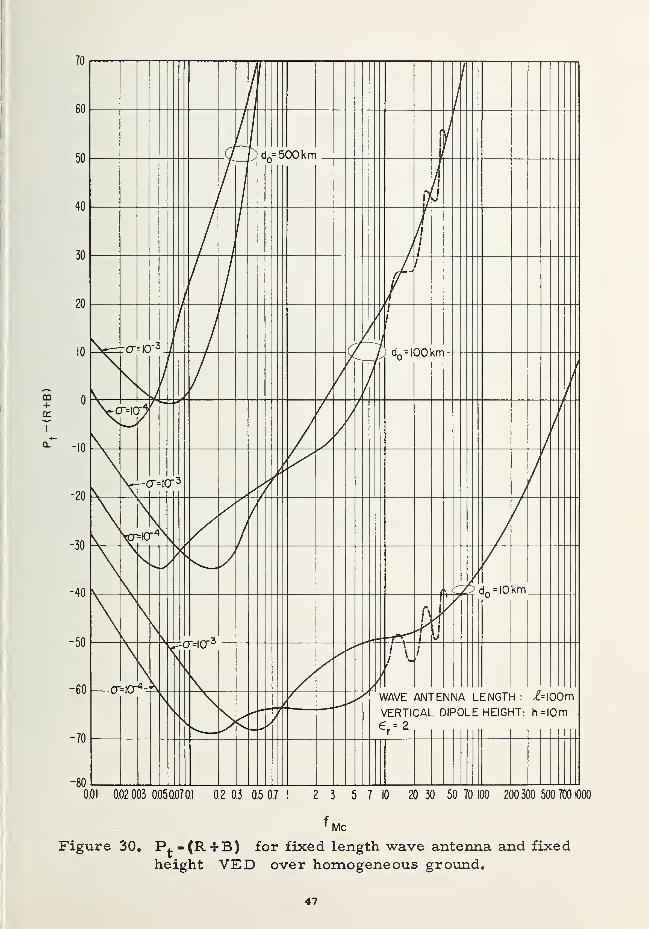
Using figures 24, 26, and 28, the quantity P - (R + B) is shown in figure 30 for the case of
a wave antenna of length I = 100 m transmitting in the optimum direction towards a short vertical
electric dipole at a height h = 10 m. For the example of standard broadcast service used pre-
viously, the required power P^_ at a range of 10 km and for a frequency of 300 kc/s would be
about 12 db or 16 w. For the low-grade voice communication service the required power at a
distance of 100 km and for a frequency of 100 kc/p would be about 30 w. At high frequencies
the estimates of P^ shown in figure 30 will be somewhat pessimistic, since a small height gain
effect will occur due to the height of the dipole. Graphs for calculating this effect may be obtained
from another paper [Vogler, 1964].
The combination of a wave antenna and dipole and the particular lengths and heights used in
the preceding example were arbitrarily chosen. As pointed out in section 1, the purpose of the
communication system together with the necessary restrictions placed on its physical components
must first be established before specific power requirements may be estimated. Combinations
of antennas other than the one assumed in the present example should be investigated before a
decision is made as to what will constitute an efficient lunar communication system.
In the particular idealized system described by figures 27 and 30, a number of points should
be noted: (1) the required power does not vary appreciably over the range of assumed, but
does depend significantly on the conductivity at low frequencies; (2) propagation out to somewhat
beyond 100 km is practical for most types of systems and service, at least at MF or below;
(3) the curves indicate an optimum frequency exists, depending on the conductivity of the lunar
surface and the range of propagation; for the model assumed and for the conductivities and dis-
tances shown, the optimum frequency lies in the LF band. It should be kept in mind that the oper-
ating noise factor of the receiving system was considered to be a function only of the galactic noise
(which, of course, is extrapolated at the lower frequencies) and a rather low receiver noise factor.
If the receiving antenna loss £ were large enough, it is apparent from (5.3) that F would have
higher values than those assumed. Also, during the lunar day, the antenna temperature t
would increase, thus making the operating noise factor even higher.
45

46
0.01 0.02 0.03 0050.0701 0.2 0.3 0.5 0.7 ! 2 3 5 7 10 20 30 50 70 100 200300 500 700
f Mc
Figure 30. P^-^R+B) for fixed length wave antenna and fixed
height VED over homogeneous ground.
47
8. CONCLUSIONS
A study has been presented concerning various aspects of lunar surface communication; it
is hoped that these results may serve as a basis for future investigations of the subject. An attempt
has been made to present the main curves in a generalized form such that, as changes and refine-
ments in our knowledge of the moon arise, the curves may still be useful in predicting lunar
communication requirements.
It is apparent that further studies, both theoretical and experimental, would be useful in the
following areas:
1. A more precise evaluation of lunar ground conductivity, together with more information
concerning layering (if any) of the materials composing the moon,
2. Further investigation into the structure and magnitude of possible lunar ionospheres,
especially the determination as to whether an ionized layer exists at the surface, and if
so, its effects on propagation at the lower frequencies,
3. Further studies of noise effects including terrestrial noise sources, noise during high
solar activity, and low frequency galactic noise,
4. Investigations of various antenna combinations, taking into account antenna ground losses
for those situations in which a ground screen will be impractical.
5. A study of knife-edge diffraction and obstacle gain effects caused by irregularities in the
moon's surface structure.
9, ACKNOWLEDGMENTS
The author gratefully acknowledges the assistance of J, L. Noble who programmed most
of the mathematical formulas used in the calculations of the many graphs appearing in this paper.
His thanks also go to K. A. Norton and J. R. Wait of the NBS Boulder Laboratories, and to
Paul S. Goodwin of Jet Propulsion Laboratory for their suggestions and guidance.
48

10. APPENDIX: INPUT IMPEDANCE OF DIPOLE ANTENNAS
It is assumed that an elementary dipole of length di is located at the origin of a cylindrical
coordinate system (p , 9, z) at a height h above an isotropic and homogeneous conducting half-
space characterized by a dielectric constant €^ and conductivity tr^. The interface between
the two media is the plane z = - h, and for z > -h the dielectric constant is assumed to be equal
to the free space value . The magnetic permeability of the whole space is taken as the free space
value |jl (MKS units are used here). In. the case of a vertical dipole, the antenna is oriented in
the z direction, whereas for a horizontal dipole the orientation is in the 0 = 0 direction. The
elementary magnetic dipole may be considered equivalent to a small circular loop with its axis in the
direction of the dipole and with an area dA = di/p^, where |3 is the free space wave number
( = 2-rr/X). For practical short dipoles having a linear distribution of current, di should be replaced
by an effective length I = dj?/2„
The electromagnetic field of an elementary dipole above a conducting plane may be obtained
from the electric and magnetic Hertzian potentials, II and II , the components of which, if the. em
vectors are referred to a cartesian coordinate system (x, y, z), satisfy the scalar wave equation2 2
(V + (3 ) II = 0 . Using the cylindrical coordinate form of the wave equation, particular solutions
are found by the method of separation of variables resulting in expressions for the II components
involving combinations of the eigenfunction
± ^X.2
- p2
zn
where X denotes the eigenvalue (following Sommerfeld's notation), J is a Bessel function of the
first kind and order n, and the C's are functions determined from the boundary conditions. These
conditions in the present instance require that the tangential components of the electric vector E
and the magnetic vector B be continuous at the interface between the two media (air and ground).
In the case of vertical dipoles, E and B may be expressed in terms of Hertzian potentials
having a z-component only. Thus in the upper medium
= n 7 = ( nd
+ nr) 7, (a-2)
vert z \ z z /
where the superscripts d and r refer to the direct or primary stimulation and the reflected or
secondary stimulation, respectively. After solving for the coefficients C through the boundary
conditions, one finds that for
i K 00
VED: nd
= —^ f J (Vp)e_ZU
°(X/u ) dX ,
ez B J o or o o
iK r N2u_ - u, ^ -(z + 2h)u
, r
(A-3)
nez TfM Jo^p>{-2-
£—i}
e °Wuo)dx,
PoJ o <-N u + u J
49

VMD: nj iKd mmz p
n -Z U
\ JQ(\p)e °(k/u
o)d\,
(A-4)
mz p
iK p ru - u
- r j (Xp) j «iu - u ~ -(z + 2h) u(X/u )d\,
o
where
Uo
=Ni
x2 - Po'Ui
=\ x2 -Pi
2
'N2 =(e
l/€p)_i(<r
l/a>S
o ) (A-5)
(3^ and p^ are propagation constants of the upper and lower media, respectively, and the K's are
amplitude factors given by
P I (dl) p a I (dA)
K = -4-2 , K = 12-2-2e 4ttw€ m 4ir
(A-6)
For horizontal dipoles, the Hertzian potentials require both an x- and a z-component. Thus,
corresponding to (A-2),
n, =n xi-n z = (n +n )x + n z,nor x z x x z
(A-7)
After solving for the C's through the boundary conditions, one obtains:
r°° -zu
\ JJXp) e (X./u )d\,
u - u . -(z + 2h)
u
HED: nd e
P J o-o o
iK. r e c j (Xp
)(_2
—
1\J o*
K '1 u + u
, jo V. o 1 >
(K/u )dX,o
iK cos9 ~ , 2(u -uj^ -(z + 2h)u , ,
-\—) V^-f-r
—
L h V/pjW'o Jo v. n u +u, J
o 1
(A-8)
HMD: fl
iKm f J (\p) e (\/u )d\,mx P J o r o
iK , N u - u, -(z + 2h)u
"fl3
f JoW ( 2 — ^ 6P o ^o N u +u
o 1
(X /PQ)d\,
iK cos9 2(u -u,)-. -(z + 2h)u?
ro o u +uo 1
2where u , u,, N , K , and K are defined in (A-5) and (A-6),
o 1 e m
(A-9)
50
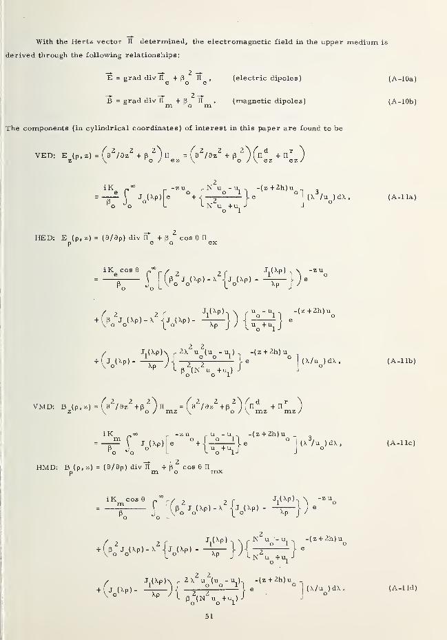
With the Hertz vector n determined, the electromagnetic field in the upper medium is
derived through the following relationships:
E = grad div n + (3 n , (electric dipoles)
B = grad div n + B fl (magnetic dipoles)mom(A-lOa)
(A-lOb)
The components (in cylindrical coordinates) of interest in this paper are found to be
2 , 2 2,„ 2 _ Z V„d „ro j \ e z e z
iK
P J oo o
J (\p)
zu r Nu -u -(z+2h)uo
e +o 1
N u +u,o 1
(X /u )dX,o
(A-lla)
HED: E (p, z) = (9/9p) div n + 3 cos 9 np 6 O 6 5t
iK cos9 „°°e r r / 2 2 r
Ji
Xpj
, J (Xp) sfu -u -(z+2h)u
2 2.J (XpK 2X u (u -u ) -(z + 2h)u
HJ»- -~-)^ ,° ° )e ° l(X/u )dX,
Xp JI 2, 2H L 6 N u +u,
o o 1
(A-llb)
,2,2 2 > / 2, 2 2\ / d rVMD: B (p,z)= 3 /9z + B )n = 9 /9z + B ) i n +n
^o / mz \ o / \ mz mz
iK co zu . u -u -(z + 2h)u° + j-i?_2le °l(X 3
/u)dX,Uo+UJ J
(A-llc)
HMD: B (p, z) = (9/9p) div n + B cos 6 np
r m r o mx
i K cos 6mCO
Jo lv
2 2f , ,
Jl(Vph
s„ Jo(x P )-x |jo
(xP )-
J(X P ) N N Uq-u -(z + 2h)u
o
o Ti
, J(XpK 2 x2u
2(u
o-u
i)
-(z + 2h)u
+w xp ) - —;{ 2 2 - J e (
W
VK ^ B ( N u + u, ) -J -1
dX
P (N ..
o o 1
(A-lld)
51

To calculate the dipole input impedance using the emf method [Wait, 1953, 1962 d; King,
1956 (p. 258) ]requires a knowledge of the axial field at the antenna. This may be obtained by taking
the limits of (A- 11) as p and z approach zero (and with 9 = 0 in the case of horizontal
dipoles). The impedance Z is then given by
VED: Z = Lim -IE (p, z) di/Ip-~o I
z
iK dl » N2u -u -2hu
-0-4 \ H 2° 6 °I (X /u )dX, (A-12a)
PoAo J o L L N u +u J J
°
o 1
HED: Z = LimJE (p, z) dl/l L
p-o I P °Jz—
o
iK die
P Io o o1
2 ruo-
un~ Zhuo\
2 2
rx u^^ u^ -ui) " 2hu -i
*{ z,z ', }• "l^V*.B N u +uj J Jo ol
VMD: Z = Lim -| coB (p, z) d A/Ip—
o
z-*o
icoK dA n°°'
r ,u -u., -2humP Io o
(A-12b)
o L o 1 J -I
HMD: Z= L,im-\ co B (p, z)dA/lp—
o
z—
o
r-,-/ 2 2, \ / rN\- u
i-i-2hu
oo*"oL ^ N u +uo 1
oe
2 2,\ u (u - u_ ) , -2hu _o o 1 ] o 1 , .~
2f
eI
(X/uJ dX ° (A-12d)(3 (N u +uj J Jo o 1
52
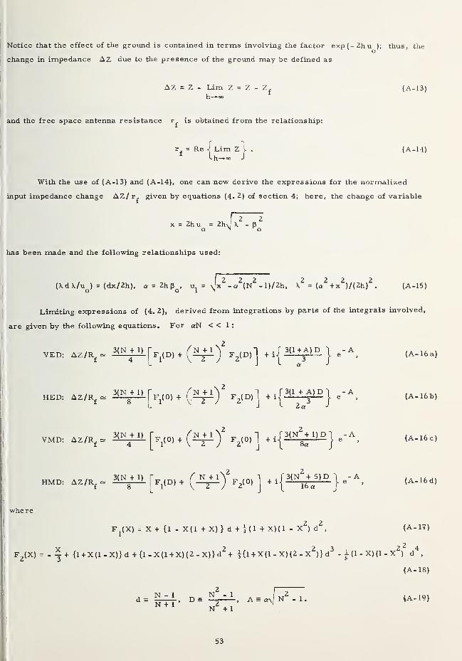
Notice that the effect of the ground is contained in terms involving the factor exp(- 2h u ); thus, theo
change in impedance AZ due to the presence of the ground may be defined as
AZ = Z - Lim Z = Z - Z, (A-13)
and the free space antenna resistance r^ is obtained from the relationship:
r = Re -i Lim ZLh^oo
(A-14)
With the use of (A-13) and (A-14), one can now derive the expressions for the normalized
input impedance change AZ/ r^ given by equations (4. 2) of section 4; here, the change of variable
2 2x = 2h u = 2h\ \ - R
o N o
has been made and the following relationships used:
(\d \/uo
) = (dx/2h), a=2hpo> ^ = \\x
Z- <*
2(N
2- l)/2h, \
Z= (c*
2+ x
2)/(2h)
2(A-15)
Limiting expressions of (4.2), derived from integrations by parts of the integrals involved,
are given by the following equations. For aN < < 1 :
2
VED: AZ/R£ «M^rFi(D)+ (Nfi F
2(D)
3(1+A)D 1 e-A
(A- 16 a)
HED: AZ/Rf^ ^-k(0) +
N + 1 . f 3(1 + A)D 1 -AF2(D)
|
+1|-L_L_ L e
L 2 a
(A-I6b)
VMD: AZ/R ^ M+ILf 4
F2(0) + 1
. f 3(N + 1)D] -A8a
(A-I6c)
HMD: AZ/Rf^ 3(N + 1) F^D) +
where
2. .2F^X) = X+ {l-X(l+X)}d + j(l+X)(l-X)d ,
(A-17)
F2(X) = + {1 + X(l-X)}d +{1-X(l + X)(2-X)}d
2+ |{1 + X(1-X)(2 -X
2)}d
3- 1 (1 - X) (1 - X
2) d
4,
(A-18)
(A-19)N - 1 „ N - 1 . 2 ,ds nTT' Ds —'ASQ
"\|N
"1
N + 1
53

For a N > > 1
(A-20a)
HED: ~ tM^H' 1 -A 2/N) +
+
- ^)} ie , (A-20b)-"
VMD: AZ/Rf~ _3_ j N-l
3 I N+l- i a
i e » (A-20c)
HMD: AZ/R V ISUc - «2- */») 4- £ (i -^ 1 1 •
- M. I^OI
f ,31 N+l f !
y
For the case of dipoles above a perfectly conducting plane (N—«>), equations (A-20) reduce to the
well-known expressions :
VED: AZ/Rf— (— {sin a - a cos a} + i {cos a + as in a} (A-21 a)
HED: AZ /R. — .
f V2a
3f {(1 - a
2) sin a - a cos a} + i {(1 - a;
2) cos a + a sin a}
j,
(A-21 b)
VMD: AZ/Rf— - f y l~{sina - a cos a} + i {cos a + a sina} "j
, (A-21 c)
HMD: AZ/Rf^-(^—
2 a
2 2{(1-a ) sin a - a cos a} + i {(1 - a )cosa+asina} (A-21 d) i
54

11. REFERENCES
Beverage, H. H. , C. W. Rice, and E. W. Kellogg (1923), The wave antenna, Trans. AIEE 42,
215.
Bremmer, H. (1949), Terrestrial radio waves, (Elsevier Publishing Co. , Amsterdam).
Brown, W. E. (I960), A lunar and planetary echo theory, J. Geophys. Res. 65, 3087.
Burrows, C. R. , and S. S. Atwood (1949), Radio wave propagation, (Academic Press Inc.,
New York, N. Y. ).
Carson, J. R. (1926), Wave propagation in overhead wires with ground return, Bell SystemTech. J. _5, 539.
CCIR (1951), Bandwidths and signal-to-noise ratios in complete systems, VI Plenary Assembly,International Radio Consultative Committee 1, 30, Geneva.
CCIR (1963), The concept of transmission loss in studies of radio systems, Documents of the XthPlenary Assembly, Recommendation 341, ITU Vol. Ill, Geneva.
Coleman, B. L. (1950), Propagation of electromagnetic disturbances along a thin wire in a
horizontally stratified medium, Phil. Mag. 41, 276.
Crichlow, W. Q. , D. F. Smith, R. N. Morton, and W. R. Corliss (1955), Worldwide radio noise
levels expected in the frequency band 10 kc to 100 Mc, NBS Circ. 557.
Daniels, F. B. (1961), A theory of radar reflection from the moon and planets, J. Geophys.Res. 66, 1781.
Elsmore, B. (1957), Radio observations of the lunar atmosphere, Phil. Mag. 2, Series 8, No. 20,
1040-1046.
Hartz, T. R. (1963), Satellite measurements of cosmic radio intensities at frequencies less than
12 Mc/s, talk given at the 1963 Spring URSI Meeting, Washington, D. C.
King, R. W. P. (1956), The theory of linear antennas, (Harvard University Press, Cambridge,Mass. ) .
Martin, C. A. , and G. S. Wickizer (1949), Study of Beverage wave antenna for use with low-frequency Loran, RCA, Final Engineering Report on Contract W-28-099-ac-315.
Menzel, D. H. (1961), Cosmic noise survey, Harvard College Observatory, Cambridge 38, Mass.
Norton, K. A. (1941), The calculation of ground-wave field intensity over a finitely conducting
spherical earth, Proc. IRE 29_, No. 12, 623-639.
Norton, K. A. (1959), System loss in radio wave propagation, J. Res. NBS 63D (Radio Prop.),
No. 1, 53-73.
Norton, K. A. (1962), Efficient use of the radio spectrum, NBS Tech. Note No. 158.
Page (1962), Utility of lunar groundwave propagation, Report PCE -R-4541 -000 1 A, PageCoirimunications Engineers, Inc. , Washington, D. C.
Senior. T. B. A., and K. M. Siegel (I960), A theory of radar scattering by the moon, J. Res.
NBS 64D (Radio Prop. ), No. 3, 217.
Vogler, L. E. (1963a), Point-to-point communication on the moon, J. Res. NBS 67D (Radio
Prop.), No. 1, 5-21.
55

Vogler, Li, E. (1963b), Lunar point-to-point communication, chapter (pp. 533-559) in Tech-nology of lunar exploration, edited by C, I. Cummings and H, R. Lawrence, (AcademicPress, New York, N. Y. ) ,
Vogler, L. E. (1964), The calculation of ground wave attenuation in the far diffraction regionRadio Sci. J. Res. NBS/ USNC-URSI 68D. No, 7, 819-826.
Vogler, L. E. , and J. L. Noble (1963), Curves of ground proximity loss for dipole antennas,
NBS Tech. Note No. 175.
Vogler, L, E. , and J. L. Noble (1964), Curves of input impedance change due to ground for
dipole antennas, NBS Monograph 72,
Wait, J. R. (1953), Radiation resistance of a small circular loop in the presence of a conducting
ground, J. Appl. Phys. 24, No. 5 S 646-649.
Wait, J. R. (1954), Radiation from a ground antenna, Can. J. Technol, 32, 1.
Wait, J. R. (1956), Effect of the ground screen on the field radiated from a monopole, IRE Trans.Ant. Prop. AP-4, 179.
Wait, J. R. (1959), Transmission cf power in radio propagation, Electronic and Radio Engineer 36,
No. 4, 146.
Wait, J. R. (1961), Private communication.
Wait, J. R. (1962 a), Electromagnetic waves in stratified media, (Pergamon Press, Oxford).
Wait, J. R. (1962b), The propagation of electromagnetic waves along the earth's surface,
chapter (pp. 243-290) in Electromagnetic waves, edited by R. E. Langer, (University of
Wisconsin Press, Madison, Wis.).
Wait, J. R. (1962 c), Introduction to the theory of VLF propagation, Proc. IRE 50, 1624-1647.
Wait, J, R. (1962 d), Possible influence of the ionosphere on the impedance of a ground-basedantenna, J. Res. NBS 66D (Radio Prop. ), No. 5, 563-569.
Wait, J. R. , and W. J. Surtees (1954), Impedance of a top-loaded antenna of arbitrary length over
a circular grounded screen, J. Appl. Phys, 25, 553,
Weil, H, , and M. L, Barasch (1963), A theoretical lunar ionosphere, Icarus 1, No. 4, 346-356.
56

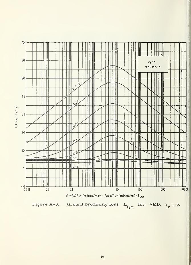
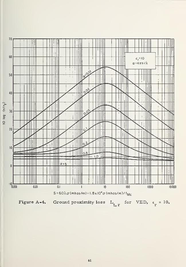
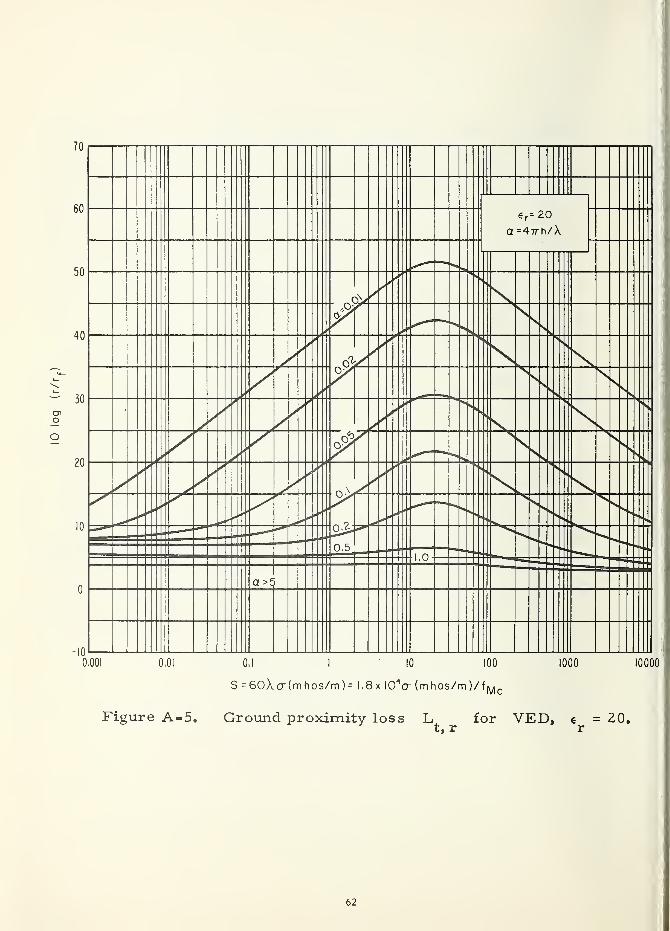
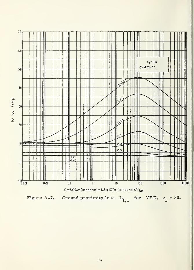
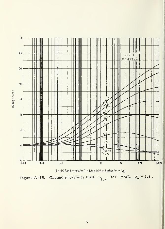
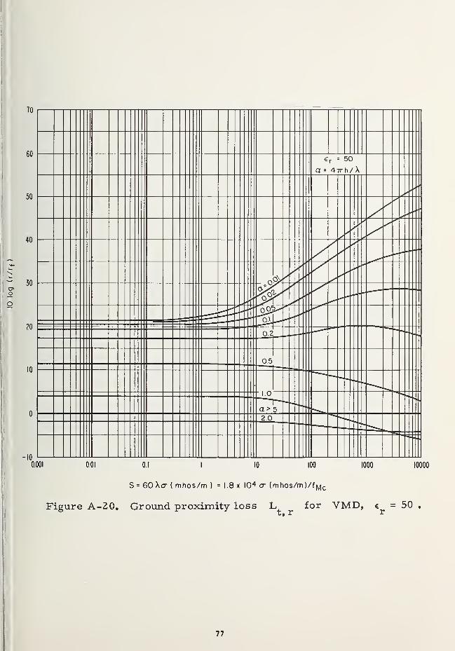
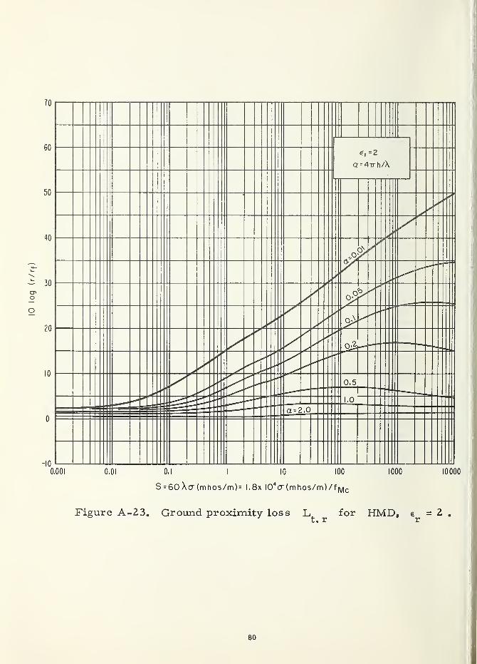
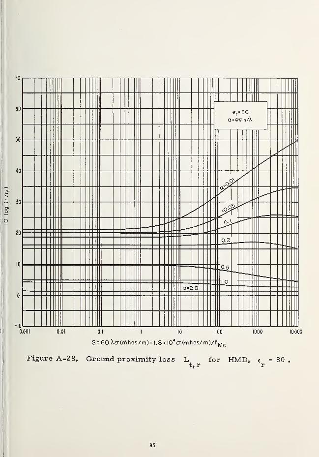
12. GRAPHS OF GROUND PROXIMITY LOSS, ^ = 10 log{r/rf)
for
Vertical Electric Dipoles (VED)
Horizontal Electric Dipoles (HED)
Vertical Magnetic Dipoles (VMD)
Horizontal Magnetic Dipoles (HMD)
s = 60 \ (T^mhos/m), a - (2h) (2tt/X.) ,
e : relative dielectric constant of groundr
cr(mhos/m): conductivity of ground
h: height in meters of antenna above ground
X.: wavelength in meters
57

58

59
60
61
62

-10
0.001 0.01 0,1 I 10 100
S = 60Xa(mhos/m)= 1, 8 x I04cr(m hos/m )/f
1000 10000
Mc
Figure A-6. Ground proximity loss L for VED, € = 50.
63
70
€r= 80
a = 477~h/\
64

f
65

66

67

68

69

70

71
72

73

74

75

76
77

70
78

79
80

TO
81

-10
0,001 0,01 0,1 I 10 100
S = 60 Xcr (mhos/m) =1 .8 x I0
4cr (mhos/m)/ fmc
1000 10000
Figure A-25. Ground proximity loss L, for HMD, € = 10 .
«2

83

70
S = 60Xcr (mhos/m)= l,8x l04cr(mhos/m)/fMc
Figure, A-27. Ground proximity loss L for HMD, € = 50 .
t, r r
85


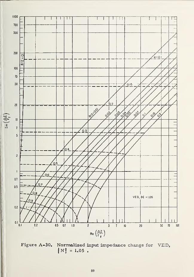
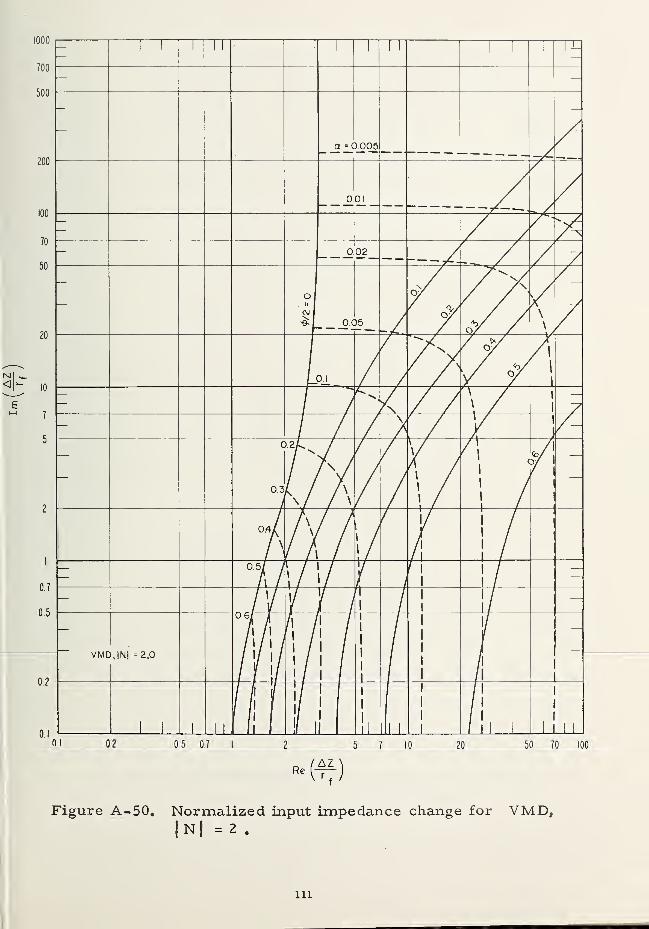
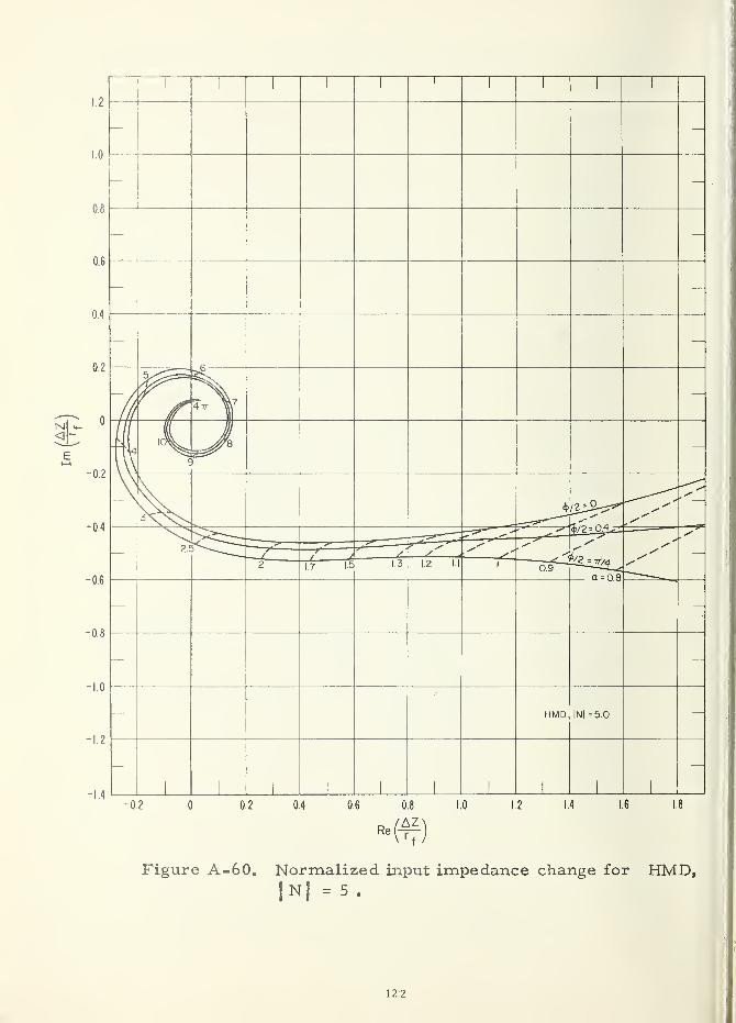
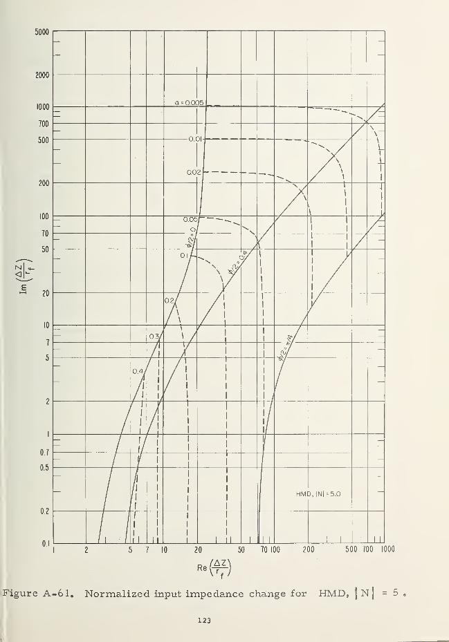
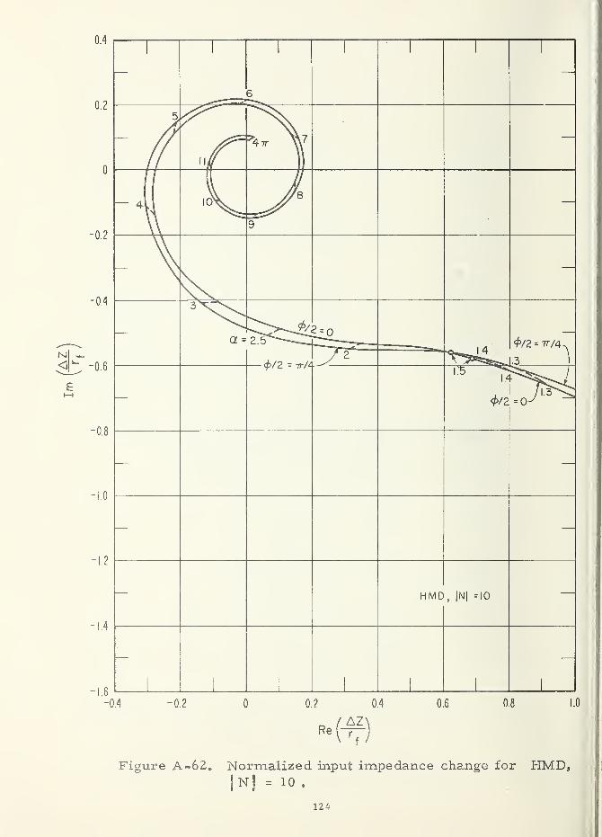
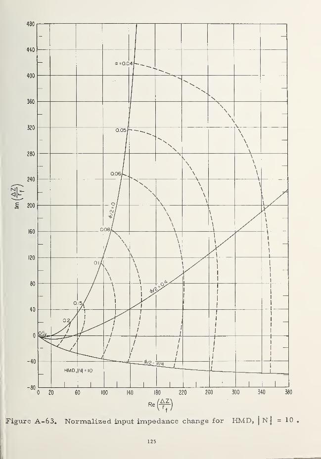
13. GRAPHS OF NORMALIZED INPUT IMPEDANCE CHANGE, AZ/r
for
Vertical Electric Dipoles (VED)
Horizontal Electric Dipoles (HED)
Vertical Magnetic Dipoles (VMD)
Horizontal Magnetic Dipoles (HMD)
|N| = 4»/2 = (^tan'^s/e ) ,r
s = 60 \ cKmhos/m), a = (2h)(2irA.) >
e : relative dielectric constant of groundr °
cr(mhos /m): conductivity of ground
h: height in meters of antenna above ground
\: wavelength in meters
87
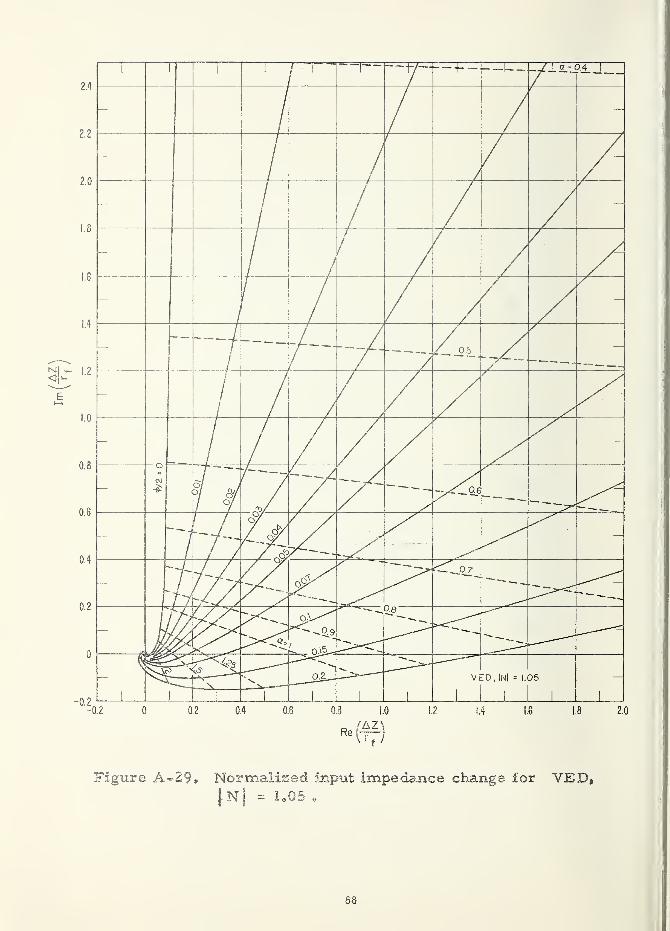
Figure A«*29. Normalised input impedance change for VED,[N] = 1.05 *
88
89

90
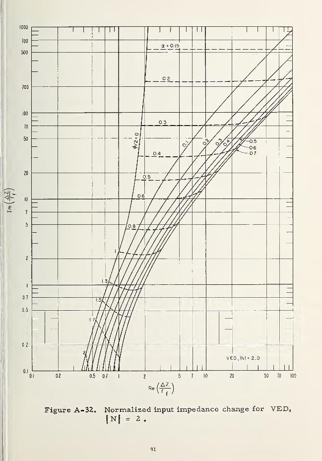
91

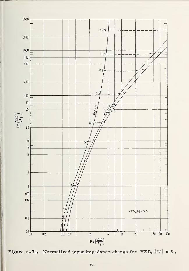
93


99
100
101

102
103
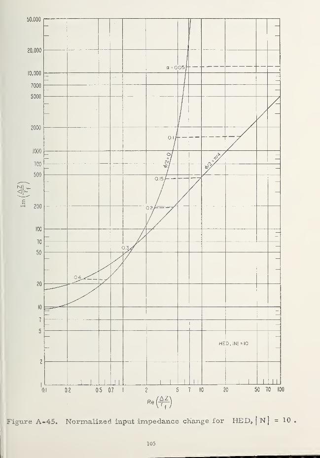
105


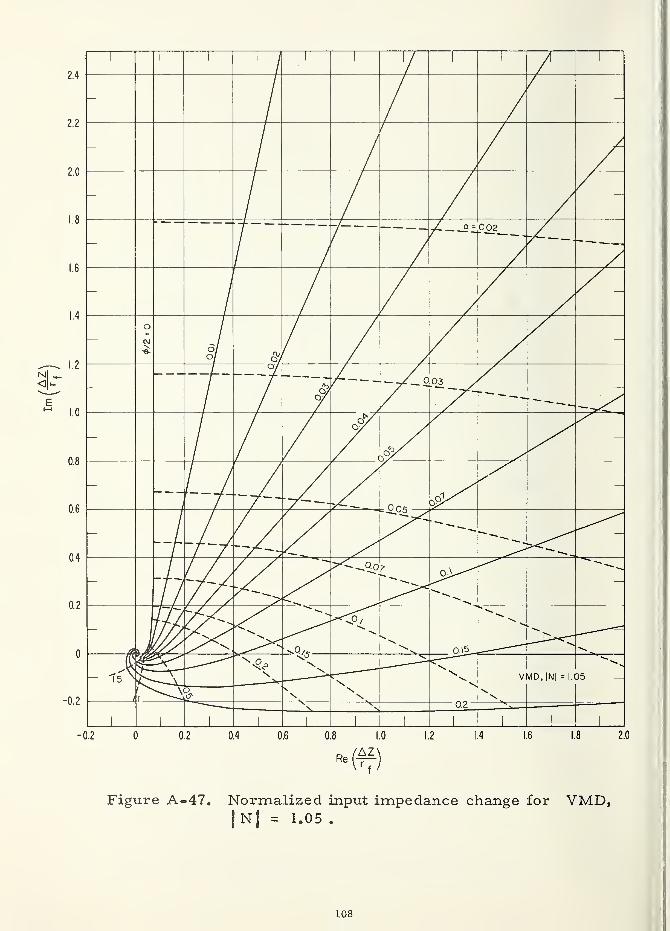
Figure A-47. Normalized input impedance change for VMD,|N| = 1.05 .
108
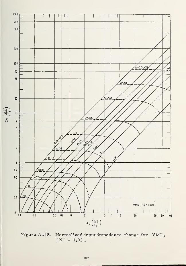
109

-0.2 0 0.2 0.4 0.6 0.8 10 1.2 1.4 16 1.8 2.0
-(f)
Figure A-49. Normalized input impedance change for VMD,|n! = 2.
no
Ill
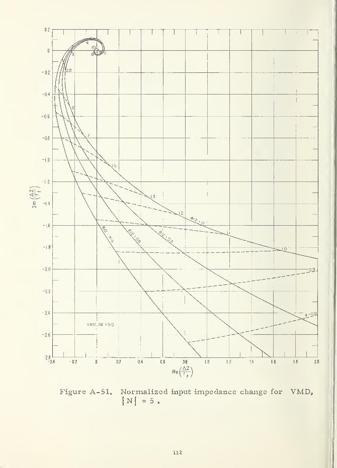
112
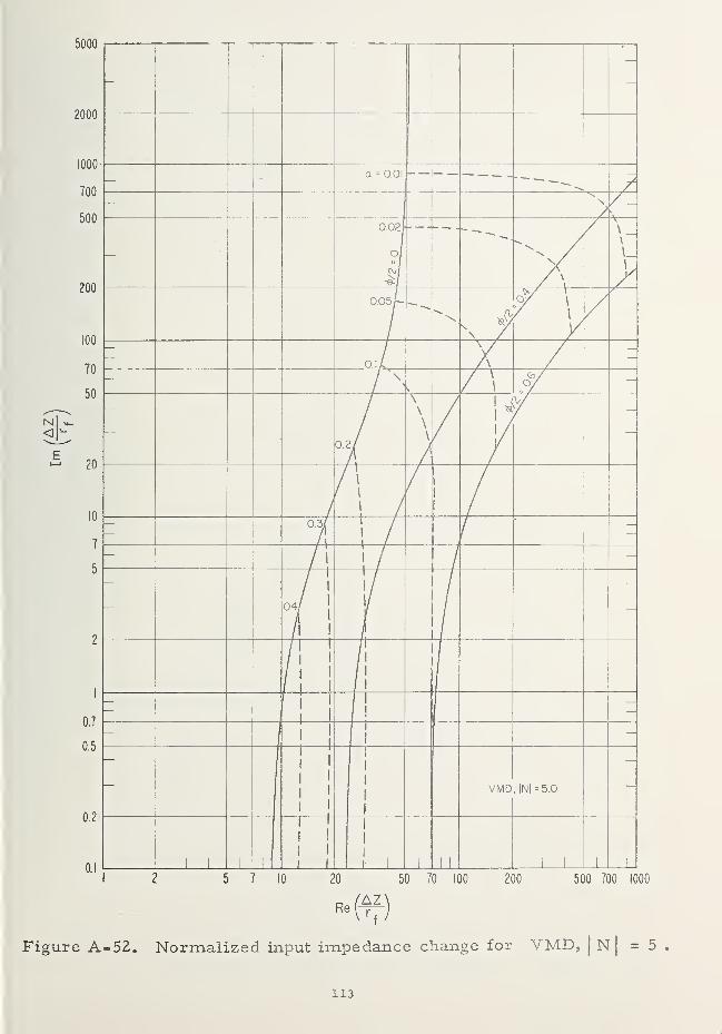
5000
2000
gure A-52. Normalized input impedance change for VMD,J
Nj =
113


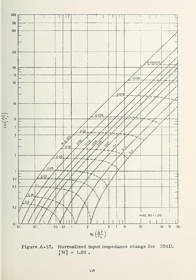
Figure A- 56. Normalized input impedance change for HMD|Nj = 1.05 .
118
119
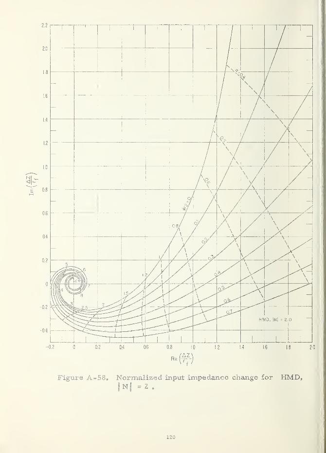
120

0.1 0.2 0.5 0.7 I 2 5 7 10 20 50 70 100
Figure A-59. Normalized input impedance change for HMD,|n| = 2 .
121
122
123
125

126
ft U. S. GOVERNMENT PRINTING OFFICE : 1964 O - 739-039