a study of high and low 'labor productivity' establishments in u.s

262 Benjamin Klotz/Rey Madoo/Reed Hansen

13 = (log L2)21 — (log L2)22,

16 = (log K)21 — (log K)22,

= (logL1 log L2)1 — (logL1 log L2)2,

Is = (log L1 log K)1 (logL1 log K)2,

19 = (logL2 IogK)1 — (logL2 log K)2. c

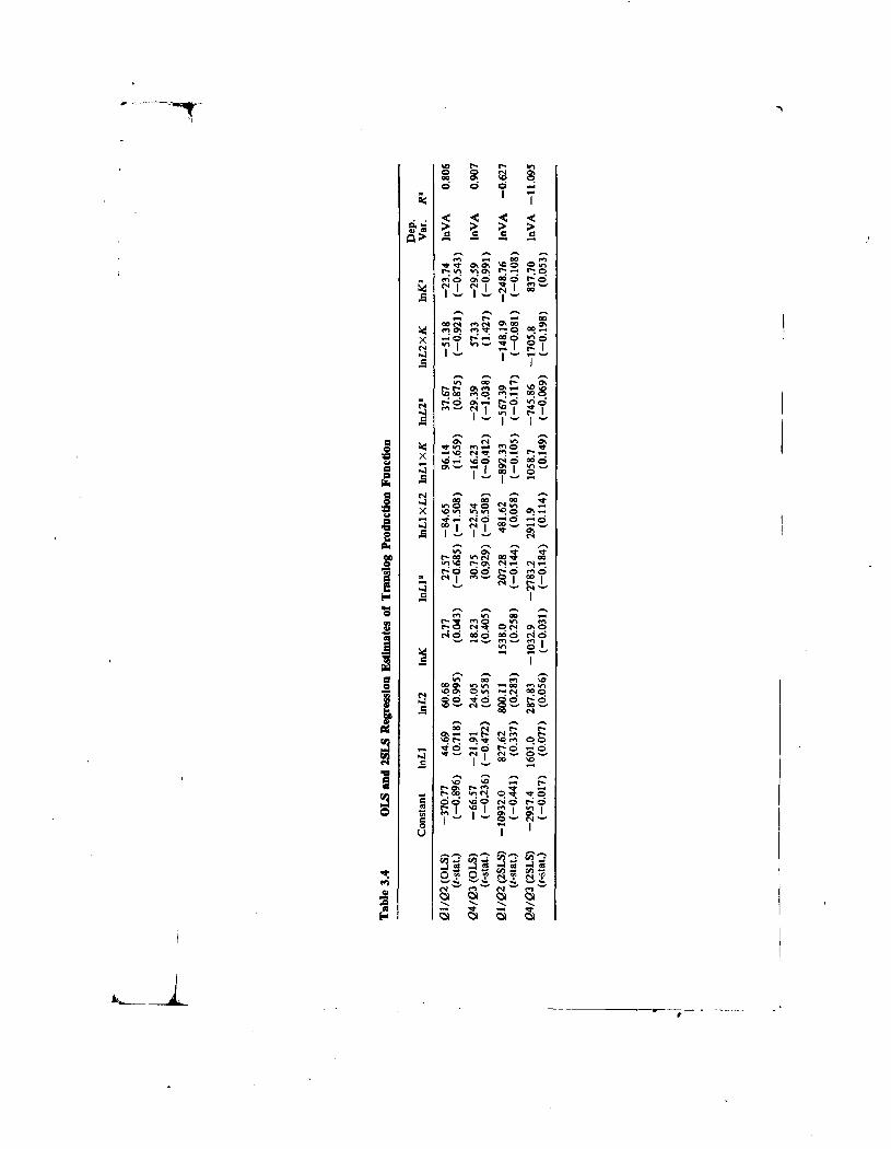
Since we assume that the production functions for quartile I and quar-tile 2 are the same, there is no problem of identifying the various pa-rameters of the structure. Input and value-added data for quartile 4 and3 establishments are combined in the same manner to form ratio van-ables and to provide estimates of parameters for the high-productivitygroup. The OLS estimates for quartile 1 (line 1 of table 3.4) indicatea good fit to the data in terms of R2 but the t statistics indicate that none

4of the nine input variables is significant at the 95% level (Jti > 1.96).This result indicates that the input variables might be highly collinear.Quartile 4 estimates have slightly higher R2 than was the case for quar-tile 1 but, again, no value exceeds 1.96.

The 2SLS estimates (lines 3 and 4) are also insignificantly differentfrom zero despite a great increase in their average value over the OLScase. The 2SLS fit is even worse than the OLS case, but this is a char-acteristic of the 2SLS approach.26

The Translog Production Function Share EquationsSince direct estimation of the coefficients of the production function

gave poor results, we did not use them to compute estimates of theAES. Instead we turned to estimation of the share equations (6). Sys-tem (6) is derived from (1) by assuming profit-maximizing behaviorby establishments. Three symmetric constraints on the share equationparameters are required:

(23) a12 = a21, a13 = a31, and a23 = a32.

Within the framework of 3SLS estimation, we can test (23). Becausethe share equations sum to unity, only two of the three share equationsare independent. The capital share equation has the worst OLS fit inboth quartile 1 and 4, so we chose to drop this equation.

Working with two share equations, only the symmetry restrictiona12 = a21 can be tested. Using 3SLS restricted estimation, we find thatthe hypothesis a21 = a12 cannot be rejected at the 95% confidence levelfor either quartile 1 or 4. In addition, restrictions (7), (8), and (23)

26. The negative R2s for the 2SLS cases are not reason for alarm because theformula for computed R2 corrected for degrees of freedom can be highly negativewhen the true R2 is close to zero.

1 263 A Study of High and Low "Labor Productivity"

imply that the sum of the three input coefficients in each share equationshould sum to zero (row homogeneity): a11 + a12 + a13 = 0 and a21+ a22 + a23 = 0. Although this zero sum does not hold exactly for theunrestricted estimates, the actual coefficient sum does not depart signifi-cantly from zero at the 95 % level of confidence.

Finally, imposing symmetry, we test to see if the production coeffi-cients of quartile 1 are significantly different from those of quartile 4 atthe 95% level of confidence. Estimates apçear in table 3.5. The resultis that we cannot reject the hypothesis that the production functioncoefficients are the same in both quartiles. In particular, although thefourth quartile intercepts appear different from the intercepts in the firstquartile, the standard errors are so large that the hypothesis of struc-tural equality cannot be rejected at the 95% level.

Computation of AES by Industry• We used equation (10) io compute the Allen partial elasticity of

substitution S, for each of the 195 industries in quartile 1 and quartile4. The calculation of individual elasticity estimates permits the exami-nation of production behavior at each individual industry observation.Because industries may not have the same production structure, thesecalculations are a check on the appropriateness of the model.

Tables 3.6 and 3.7 present the own AES estimates for quartiles 1

and 4 based on coefficient estimates obtained using 3SLS with rowhomogeneity and cross equation symmetry restrictions imposed. We

Table 3.5 3SLS (with restrictions) Regression Estimates ofTranslog Two-Input Equation System

Equation Constant lnL2 ltiK InLi Dep. Var.

Quartile 1 (3 SLS withrestrictions)

Share 1(1-stat.)

13.586(0.902)

1.835(0.417)

—14.675(—5.145)

12.841(2.396)

Share Li

Share 2(1-stat.)

43.207(4.791)

—14.675(—5.145)

14.161(4.555)

(0.515)(0.209)

ShareL2

Quartile 4 (3SLS withrestrictions)

Share 1(f-stat.)

39.146(11.173)

10.856(9.882)

—3.700(—4.531)

—7.156(—6.686)

ShareLl

Share 2(1-stat.)

38.198(15.482)

—3.700(—4.531)

9.244(12.450)

—5.544(—7.726)

Share L2

NOTE: Each two-equation system is restricted for row homogeneity (the sum ofindependent variable coefficients is equal to zero) and cross equation symmetry.

note that the resulting own AES based on these coefficients vary overa wide range. The conditions of the model require that all own AES benegative but, for example, in quartile 1, 58 of the 195 own AES repre-senting nonproduction workers, S22, were positive. The same applies forquartile 4 in which there are 64 positive estimates associated with S22.The remaining AES estimates also have numerous positive values. Tak-ing these estimates on their face value, the evidence is overwhelmingthat the conditions for existence of the model we have imposed are notmet in each industry.27

But the median values for all own AES estimates in both quartilesare negative and hence acceptable to the model specification. The bot-tom row of tables 3.6 and 3.7 indicates that median values for S11 andS22 are larger in quartile 4, while the S33 median is larger in quartile 1,suggesting greater substitution possibilities for labor in high-productivityestablishments.

1

27. In this context we are speaking in the general sense of the suitability ofour model of equilibrium behavior and the translog specification, or both.


Table 3.6 Frequencyacross 195

Distribution of Allen Elasticity of Substitution (AES)Industries (based on 3SLS estimation with restrictions)

AES Intervals S11 Quartile 1 S22 Quartile 1 Quartile 1

10.0+ 6 (6) 52 (52) 8 (8)

5.01 10.00 4 (4) 5 (5) 1 (1)

0.01 — 5.00 42 (42)- 1 (1) 3 (3)

— 0.99 — 0.0 13 (13) 0 2 (2)

— 1.99 — 1.0 47 0 28 (28)

— 2.99 — 2.0 45 3 (1) 52 (15)

— 3.99 — 3.0 14 4 39 (4)

— 4.99 — 4.0 5 7 (2) 20 (4)

—5.99 —5.0 4 5 9—6.99 —6.0 1 9 (1) 9

— 7.99 — 7.0 1 6 1

—8.99 —8.0 3 9 7

—9.99 —9.0 1 8 3

—19.99 —10.0 5 39 (2) 6

—20.0

orless 4 46 7

Approx. MedianAES —1.68 —8.50 —3.09

NOTE: Bracketed values represent the number of industries where calculated valuesfor the bordered Hessians are positive and which are unacceptable for the specifica-tion of the model we have imposed. Unfortunately, we have no way of judgingwhether the interval around these estimates may contain negative values as well.

S11 =production workers; = nonproduction workers; 533 =capital.

4

I—


Distribution of AllenIndustries (based on

Elasticity of Substitution (AES)3SLS estimation with restrictions)

AES Intervals S11 Quartile 4 Quartile 4 S33 Quartile 4

10.0+ 205.01 10.00 1

0.01 5.00 1

— 0.99 0.0 1

— 1.99 — 1.0 2— 2.99 — 2.0 5— 3.99 — 3.0 7— 4.99 — 4.0 11— 5.99 5.0 9— 6.99 6.0 20— 7.99 7.0 18— 8.99 8.0 18— 9.99 9.0 10—19.99 —10.0 46

—20.0or less 27

(12) 58(1) 5(1) 1

(1) 0(2) 1

(3) 0(3) 1

(4) 3

(4) 2(10) 2(2) 9(4) 7(1) 3

(3) 48

(9) 60

(45) 1

(5) 0(1) 9

49(1) 115

14(1) 5(2) 0(1) 1

00

(1) 00

(2) 1

(2) 0

(1)

(49)(9)(1)(1)

Approx. MedianAES —8.14 —12.19 —1.35

NoTE: Bracketed values represent the number of industries where calculated valuesfor the bordered Hessians are positive and which are unacceptable for the specifica-tion of the model we have imposed. Unfortunately, we have no way of judgingwhether the interval around these estimates may contain negative values as well.

S11 = production workers; S22 =noaproduction workers; = capital.

Cross-elasticity of substitution estimates based on the Allen formula-tion were also calculated, and are given in tables 3.8 and 3.9. In quartileI positive values occur for the median estimates of S12 and S23, and onecross-elasticity term (S13) is negative. In quartile 4, based on mediancross-elasticity estimates, all pairs of inputs exhibit positive cross-elas-ticity effects. Positive effects imply that inputs are substitutes and nega-tive effects imply that inputs are complements. Again, the evidencesuggested by central measures is that the two quartile groups are dif-ferent.

This completes the AES analysis, and we now turn to a study of theown and cross price elasticity of demand for production inputs.

Own Price Elasticities of DemandThe own AES estimates in tables 3.6 and 3.7 lead directly to the

computation of own price elasticities (OPE) of demand:OPE estimates for all inputs (not shown)

is less dispersed than that of the AES estimates, the dispersion beingcompressed by the share weighting factor. The median OPE estimates

265 A Study of High and Low "Labor Productivity"

is)

isI.g1.

r

r

I



Elasticity of3SLS estimati

Substitution (AES)on with restrictions)

AES Intervals S12 Quartile 1 S13 Quartile 1 S23 Quartile 1

10.0+ 30 6 (6) 165.01 10.00 40 3 (3) 190.01 5.00 65 (5) 56 (56) 107 (12)

— 0.99 — 0.0 6 (6) 87 15 (15)— 1.99 — 1.0 6 (6) 18 7 (7)

— 2.99 — 2.0 6 (6) 7 8 (8)— 3.99 — 3.0 6 (6) 4 3 (3)

— 4.99 — 4.0 3 (3) 1 2 (2)

— 5.99 — 5.0 3 (3) 2 3 (3)— 6.99 — 6.0 3 (3) 1 3 (3)— 7.99 — 7.0 2 (2) 1 1 (1)— 8.99 — 8.0 3 (3) 0 2 (2)—9.99 —9.0 0 1 0—19.99 —10.0 12 (12) 4 4 (4)

—20orless 10 (10) 4 5 (5)

Approx. Median

AES 2.89 —0.37 2.08

NOTE: Bracketed values represent the number of industries where calculated valuesfor the bordered Hessians are positive and which are unacceptable for the specifica-tion of the model we have imposed. Unfortunately, we have no way of judging

whether the interval around these estimates may contain negative values as well.S11 workers; S22 =nonproduction workers; S33 = capital.

shown in table 3.10 are mostly larger in quartile 4 than in quartile 1,They differ substantially in the case of nonproduction labor and mildlyin the case of capital. In the case of production labor (E11) they arereasonably concentrated about the median of —0.94 for quartile 1,while they are somewhat more dispersed about the median of —1.15for quartile 4. The median value for nonproduction labor (E22) is—1.23 for quartile 1 and —2.00 for quartile 4. The median OPE forcapital is —0.58 for quartile 1 and —0.63 for quartile 4.

Cross Price Elasticities of DemandThe cross price elasticity of demand estimates are computed for pairs

of inputs by a generalization of the OPE formula, and are denoted byCPE:

(24) =We mention only a few of the size comparisons for median values ofquartiles among factors, since OPE will take on the sign of the respec-tive AES. Median CPE estimates for quartile 4 are all positive. All


Ti4




Elasticity of Substitution (AES)3SLS estimation with restrictions)

AES Intervals S12 Quartile 4 S13 Quartile 4 S23 Quartile 4

10.0+ 42 6 (4) 9 (1)5.01 10.0 40 9 (6) 20 (6)

0.01 5.0 52 156 (42) 129 (27)

— 0.99 0.0 1 (1) 7 (2) 19 (17)

— 1.99 — 1.0 2 (2) 6 (3) 3 (1)

— 2.99 — 2.0 2 (2) 1 (1) 1 (1)

— 3.99 — 3.0 5 (5) 4 (3) 3 (3)— 4.99 — 4.0 1 (1) 1 1 (1)

—5.99 —5.0 6 (6) 0

— 6.99 — 6.0 4 (4) 3 (1)

— 7.99 — 7.0 3 (3) 1

—8.99 —8.0 5 (5) 1

— 9.99 — 9.0 3 (3) 3 (1)

—19.99 —10.0 8 (8) 2 2 (2)

—20.0

orless 21 (21) 3

Approx. MedianAES +3.51 +2.35 +2.35

NOTE: Bracketed values represent the number of industries where calculated valuesfor the bordered Hessians are positive and which are unacceptable for the specifica-tion of the model we have imposed. Unfortunately, we have no way of judgingwhether the interval around these estimates may contain negative values as well.

= production workers; S22 =nonproduction workers; 533 = capital.

Table 3.10 Median Elasticity of Substitution of 195 Industries(based on 3SLS estimation with restrictions)

Elasticity Measure Quartile 1 Quartile 4

Own price elasticity of substitutionProduction workers (E11)Nonproduction workers (E22)Capital (E33)

—0.94—1.23—0.58

—1.15—2.00—0.63

Cross price elasticity of substitutionProduction workers—nonproduction workers (E12)Production workers—capital (E13)Nonproduction workers—capital (E23)

1.87—0.34

0.40

0.980.490.39

inputs are substitutes. In quartile 1 the median CPE for productionworkers and capital (E13) is negative at —0.34. Thus, unlike quartile4', capital and production workers are complements. The fnedian CPEfor production workers and nonproduction workers is positive at 1.87,

26$ Benjamin Klotz/key Madoo/Reed Hansen

indicating that they are substitutes. The median estimate of the CPE fornonproduction workers and capital is 0.40 in quartile 1.

In the next section we report the estimates from the analysis of atranslog average cost function which uses price variables as inputs.

The Share Equations of a Translog Cost FunctionIn this part of the study we estimate the parameters of a translog cost

function due to Christensen, Jorgensen, and Lau (1973), under theassumption of constant returns to scale. As demonstrated in (12)—(18),the estimating forms of the share equations also appear in the logs ofthe variables, but, unlike the profit-maximizing model, with the produc-tion function as the starting point, they are functions of input prices andnot functions of input levels.

We separately tested for cross equation symmetry and linear homo-geneity and found that the test restrictions were not rejected at the 95%level. Symmetry and homogeneity restrictions were then imposed andthe system reestimated to provide estimators of Allen partial elasticitiesof substitution (AES). Table 3.11 summarizes the results of the regres-sion estimation. The coefficient estimates are in general poor.

We computed the Allen partial elasticities anyway and evaluatedthem at the mean level of a quartile class according to formula (22):

when

1

Our results on the own and cross AES estimates are reported in table3.12. Since all cross elasticity estimates are positive, no significant corn-plementarity between inputs is indicated. In addition, all own-elasticitymeasures have the appropriate negative sign.

In table 3.12, the own AES estimates differ considerably between thetwo quartiles. Estimates corresponding to S11 and 522 in quartile 4 are6 times and 2 times larger than their first-quartile counterparts. Thevalue for S33 in quartile 1, however, is 6 times greater than in quartile4. Table 3.13 gives the corresponding estimates of the OPE for the threeinputs, and for comparison we repeat the results of OPE estimates ob-tained via the production function route in table 3.14. The estimatesfrom both specifications are remarkably close. The clear pattern thatemerges, except for E33, is that quartile 4 effects are more elastic thanquartile 1. This completes the analysis of translog specifications of tech-nology differences.

e

f

Table 3.12 Allen Partial Elasticities of Input Substitutionacross 195 Industries (based on 3SLS estimationwith restrictions)

Quartile Own Cross

1 S11=— 0.795.99

S33_— — 6.31 S23=

1.820.910.96

4 S11=— 6.214S22=—11.70

0.03Sj;=

1.991.661.74

NoTE: OPE estimates obtained from two-input price shares equation system.

Within the cost function framework, an attempt was made to see ifeconomies of scale could be a possible explanation for differences inproductivity between the two quartiles. In carrying out this test weadded a proxy variable for scale, the log of man-hours of productionworkers, to the share equations.28 Using 3SLS with all restrictions im-

28. This new share equation system would result if we postulated a translogaverage cost function with nonconstant returns to scale [CfQ = f(p1, p2. Q)],and derived its share equations as in (12)—(18).

p


a

•1Table 3.11 3SLS (with restrictions) Regression Estimates ofTranslog Two-Input Price Shares Equation System

Constant in Wi In W2 hi VK Dep. Var.

Quartile 1 (3 SLS withrestrictions)

Share 1 48.555 —11.006 11.722 —0.716(I—stat.) (8.863) (—1.307) (1.386) (—4.117)

ShareLl

Share 2 25.261 11.722 —11.608 —0.113(1—stat.) (5.287) (1.386) (—1.366) (—1.108)

ShareL2

Quartile 4 (3SLS withrestrictions)

Share 1 36.823 —12.140 2.826 9.314(1—stat.) (4.123) (—2.525) (0.575) (2.115)

Share LI

Share 2 28.501 2.826 —9.255 6.429(1—stat.) (3.540) (0.575) (—1.441) (1.880)

Share L2

NOTE: Each two-equation system is restricted for row homogeneity (the sum ofindependent variables coefficients is equal to zero) and cross equation symmetry.

Table 3.13 Own Price Elasticity of Demand for Inputsacross 195 Industries (based on 3SLS estimationwith restrictions): Cost Function Estimates

Quartile 1Quartile 4

E11= —0.51 E22= —1.31E11= —1.35 E22= —1.56

E33 = —0.81E33= —0.02

Quartile 1Quartile 4

E22=—1.23E22=—2.00

E11=E11=

0.941.15

E53= —0.58—0.63

NOTE: OPE estimates obtained from two-input price shares equation system.

posed, none of the coefficients of the scale variable were significant,suggesting that scale does not explain differences in labor shares anddifferences in labor productivity among quartiles or industries.

3.6.3 Monopoly and Growth Considerations: A FurtherSingle-Equation Experiment

The 3SLS estimates of the three translog share equations (6) indicatethat none of the corresponding coefficients differ significantly (at the95% level) between quartiles 1 and 4. However, in general, our esti-mates are not very precise, and we had to appeal to average measuresin many cases for the experiment to make economic sense. The theo-retical specification appears to be too rich for the data we have on ourhands. We speculate, therefore, that quartile 1 data, especially, maycontain much "noise" and are not explainable by a static productionmodel. The divergence of coefficients may indicate that correspondingparameters of the translog production function really differ between thequartiles, or perhaps it may indicate that the input shares of establish-ments in the two quartiles did not arise from long-run equilibrium condi-tions in 1967. This latter possibility is worth investigating because, dueto the ranking of plants by their productivity, establishments may appearin the top quartile not only because they have normally high produc-tivity but also, as mentioned previously, because they may be the bene-ficiary of favorable economic events which have added a positive transi-tory component to their value added per production worker man-hour.Similarly, bottom-quartile plants may, on the average, have some nega-tive transitory components in their 1967 productivity. A positive com-ponent in the value-added productivity of quartile 4 plants will lift theircapital share above, and reduce their labor shares below, the long-run


NOTE: OPE estimates obtained from two-input price shares equation system.

Table 3.14 Own Price Elasticity of Demand for Inputsacross 195 Industries (based on 3SLS estimationwith restrictions): Production Function Estimates


levels. Conversely, a negative transitory element in quartile 1 establish-ments will depress their capital share below, and push their labor sharesabove, true equilibrium amounts.

The disequilibrium hypothesis cannot be checked directly because alongitudinal sample of plant data is unavailable to us. Instead, asproxies for quartile disequilibrium, we need unpublished Bureau ofLabor Statistics data on the past (1958—67) trend of growth rates inindustry shipments, shipments per man-hour (productivity), and ship-ment prices. In this instance output was defined as value of shipmentsdeflated for price changes, and productivity was defined as deflated

— shipments per man-hour of production workers. In order to discover8 which of the three growth-rate variables was the most important mdi-3 cator of disequilibrium we added all three to our previous multiple

regression equation intended to explain interquartile productivity differ-entials. The equation is reproduced in table 3.15 along with the effectsof adding the growth-rate variables. Table 3.15 indicates that the pastrate of productivity increase in an industry is significantly related to itsproductivity differentials, not only between quartiles 4 and 3 but alsobetween quartiles 3 and 1. This suggests that a group of leading plantsexperience productivity surges that tend to outstrip the industry averageand to drag up the average as well. And, in addition, the acceleratingaverage leaves the low-productivity establishments even further behind.The strong effect of past productivity advance upon productivity differ-entials suggests that, at some point, the plants that fall into eitherquartiles 1 or 4 are out of equilibrium, the former group being belowtheir long-run level of productivity and the latter set being above it.29

The past rate of price increases in an industry also has a significantlypositive influence on interquartile productivity differences. Perhaps thisis due to unequal shifts in the demand for specific plants' products thatallow these establishments to increase prices by more than their com-petitors. Or price increases may be due to monopoly power, in whichcase they would be associated with productivity differentials flowingfrom the same source. We will discuss this possibility shortly.

The third growth-rate variable, that of shipments, has a significantlynegative effect on productivity differentials. More rapid expansion ofdemand for an industry's products may allow productivity laggards tocatch up somewhat with their higher productivity competitors, perhapsbecause of a relatively faster expansion of sales which lifts their capacityutilization and their labor productivity.

All three growth-rate variables have an influence on productivitydifferentials between quartiles 1 and 4, and these differentials in turn

29. This conclusion is consistent with the erosion of plant productivity differ-entials through time noticed in seven of eight industries studied by Klotz (1966).

Tabl

e 3.

15M

ultip

le R

egre

ssio

n A

naly

sis o

f Int

erqu

artil

e Pr

oduc

tivity

Diff

eren

tials

Prod

uctiv

ityD

iffer

entia

lC

onst

ant

%A

(K/F

f)%

iWS

Iog(

P/C

)lo

g(C

on.)

R2

Qua

rtile

4to

quar

tile3

Perc

enta

gedi

ffer

ence

.559

(3.6

).1

05(0

.5)

.158

(3.6

).1

54(3

.7)

.066

(1.5

).0

79(1

.8)

— .0

34(—

1.0)

—.0

32(—

1.0)

.029

(1.1

)—

.007

(—0.

2)

— .0

15(—

0.1)

— .0

13(—

0.1)

.045

(3.3

)—

.009

(—1.

9).0

48(4

.2)

— .0

85(—

2.0)

.046

(1,7

)

.080

.170

Qua

rtile

3 to

quar

tile

1Pe

rcen

tage

diff

eren

ce

.388

(1.9

).1

79(0

.6)

.061

(1.1

).0

42(0

.8)

.067

(0.9

).1

34(1

.8)

.130

(1.1

).1

08(0

.9)

.078

(1.7

).0

59(1

.3)

.261

(1.5

).1

57(0

.9)

.047

(1.9

)—

.021

(—2.

6).0

70(3

.5)

.049

(0.7

).0

67(1

.4)

.028

.107

t val

ues

base

d on

195

obs

erva

tions

: t=

1.6

5(9

0% c

onfid

ence

); e

=1.

97(9

5% c

onfid

ence

)V

aria

bles

:K

/H =

capi

tal

per p

rodu

ctio

n w

orke

r man

-hou

rN

IL =

nonp

rodu

clio

nw

orke

rs p

er p

rodu

ctio

n w

orke

rW

=ho

urly

wag

es o

f pro

duct

ion

wor

kers

H =

prod

uctio

nw

orke

rs m

an-h

ours

Spr

oduc

t spe

cial

izat

ion

ratio

P =

pric

eof

ship

men

tsV

S =

valu

eof

ship

men

tsV

S/H

=sh

ipm

ents

per p

rodu

ctio

n w

orke

r man

-hou

rE/

Cpl

ants

per

com

pany

Con

. =C

once

ntra

tion

ratio

(per

cent

of s

hipm

ents

in fo

ur la

rges

t com

pani

es)

——

— -

' —-

p,


are associated with disparities in input shares between the quartiles.Thus, the growth-rate variables should be incorporated into the translogshare equations in some manner. But the differential impact of the vari-ables suggests that they may have a multiplicative, rather than an addi-tive, effect on input shares. In this instance, each input variable in theshare equations should be multiplied by some correction factor, whichwould be a weighted average of the past growth rates of industry out-put, productivity, and prices. The problem with this approach is thatthe weights are unknown.

In addition to disequilibrium elements, monopoly power may causedifferences in the estimated coefficients of comparable share equationsbetween quartiles 1 and 4. If quartile 4 establishments tend to have lesselastic product demand than their quartile 1 competitors, then the capi-tal share (measured as a residual in this study) will be larger in quartile4, even if both groups of plants use the same technology and factorproportions. Conversely, because factor shares add to unity, the laborshare of the quartile 4 group of plants will be less than in quartile 1.

Although monopoly affects the capital and labor share equations, wecannot incorporate it directly into the share estimates because the elas-ticity of product demand is unknown. However, two proxies for mo-nopoly power were chosen for analysis: the industry concentration ratio(the fraction of industry shipments accounted for by the four largestcompanies) and the intensity of multiplant companies (the ratio ofestablishments to firms in the industry). Both should be positively re-lated to the degree of monopoly in an industry, and the greater thisdegree the greater the chance that productivity differentials could occur.Table 3.15 indicates that the concentration ratio was significantly related(with 90% confidence) to the magnitude of the productivity differentialbetween quartiles 4 and 3, but the ratio was less successful in explainingthe quartile 3—quartile 1 discrepancy. This result suggests that high-productivity plants may belong to firms with market power while theirlow-productivity competitors have little market impact and may tendto act more like pure competitors: quartile 4 plants may belong tocompanies who are price makers, while quartile 1 establishments maytend to be owned by firms who are price takers. This explanation isconsistent with the previous finding that, ceteris paribus, productivitydifferentials are wider in industries with larger past rates of price ad-vance. The multiplant variable for monopoly power did not perform aswell as the concentration ratio, being insignificant in the quartile 3—quartile 1 comparison and having a negative influence on the quartile4—quartile 3 difference.

Summarizing the multiple regression results of table 3.15, we notethat, although R2s were low in all cases, the addition of both equilib-rium and monopoly variables doubled the goodness of fit of the top-

274 Benjamin KloIz/Rey Madoo/Reed Hansen

quartile equation and quadrupled that of the bottom quartile. Theseadded variables did not appreciably alter the coefficients of the factorproportion variables (capital per man-hour and nonproduction workersper production worker) in the top-quartile equation, and they madethese coefficients more significant statistically. On the other hand, theadded variables decreased the coefficient of capital per man-hour, whileincreasing that of nonproduction workers per production worker, in thebottom-quartile equation; the t statistics moved accordingly. In addition,the returns to scale proxy variable (production worker man-hours)becomes insignificant in both quartile equations with the addition of

4monopoly and disequilibrium variables. This behavior seems to suggestthat a production function explanation of the top-quartile productivitydifferential is more reliable than a similar explanation of the bottom-quartile difference. Our results also indicate that the incorporation ofdisequilibrium and monopoly elements into the translog share equationsmight move the estimated coefficients of comparable share equations,between high and low-productivity plants, closer together. Supposingthe parameters of comparable share equations to be the same, the onlytechnical difference among plants would then occur in the interceptterms a0 of their translog production function (1). This term, which isnot estimated by the share equations, would be an index of technicalability rather than allocative wisdom. In this case the three majorsources of interquartile productivity dispersion would be differences inpure technical efficiency, transitory disturbances in establishment pro-ductivity, and monopoly power.

3.7 Summary and Conclusions

Estimates from a theoretical formulation based on the translog pro-duction function and multiple regression analyses both indicate thatfactor proportions, represented by capital per man-hour and nonproduc-tion workers per production worker, contribute toward an explanationof high productivity in manufacturing establishments. But these factorsare less successful in explaining the level of low-productivity plants.Monopoly power also seems to be more important in explaining high,as opposed to low, productivity.

In addition to factor proportions and monopoly power effects, bothhigh and low-productivity establishments in 1967 appear to be out ofequilibrium. Their outputs, and possibly their inputs, seem to containsignificant transitory elements that depend on the past growth rates ofindustry output, productivity, and prices. These elements appear to bestrong enough to cast doubt on any static formulation of productivity

4

differences.


In all of our regression experiments with interquartile productivitydifferences, unexplained factors buried in the residual were most notice-able. The combined effect of factor proportions and monopoly powerexplained only 17% of the quartile 4—quartile 3 productivity variation,and only 11 % of the quartile 3—quartile 1 differential, across 195 in-dustries. Differences in managerial quality and in product (at the fiveand seven-digit level of disaggregation) may be responsible for muchof the residual variance. On the other hand, the low R2s of the produc-tivity equations may have been due to our poor proxies for measuringdisequilibrium effects.

Klotz (1966) found that industries differ in the extent to whichtheir high and low-productivity plants move toward the industry meanthrough time. This regression can be due to a competitive tendency toequalize their factor proportions, plus the attrition of their initial transi-tory components in output and inputs. These two effects can only beisolated and measured by tracing specific groups of high and low-pro-ductivity establishments in an industry over a period of years, whilerelating their differential productivity growth to their initial productivitylevel and the changes in their factor proportions. Ideally, for this under-taking, the analyst needs a longitudinal data set on each industry inwhich annual production statistics on specific groups of plants are re-corded for a number of years. Such a data set would permit investigationof the dynamics of plant productivity growth, and knowledge of thedynamics of the situation would allow separation of the long-run causesof establishment productivity differentials from the transitory distur-bances. The long-run causes are of most interest because the transitoryforces are probably random and uncontrollable. We conclude, therefore,that due to the power of short-run disturbances in plant productivity,cross-section data for one year, such as those analyzed in this study,are of limited use for analyzing establishment differentials.

Since the preparation of data at the plant level is an expensive oper-ation and census studies are years apart, we conclude with a few remarksas to how the usefulness of cross-section data can be improved. First,to analyze interquartile productivity differentials, the statistical theoryof ranking bias (Harman and Burstein 1974) requires that plants beranked not by a productivity measure but by a variable that is a primecause of productivity. Such a ranking would reduce the difficulty ofmeasuring transitory forces affecting particular groups. The best candi-date for a causal variable may be capital per production worker man-hour. We therefore suggest that establishments be ranked by their capitalper production worker man-hour in any future tabulations designed toanalyze productivity differences. In addition, according to the rankingtheory in Harrnan and Burstein (1974), the best ordering of plants is by

276 Benjamin KlotzfRey Madoo/Reed Hansen

a variable most strongly related to long-run productivity but not corre-lated with the transitory component. This variable might be a measureof plant productivity predicted from an equation estimated by regressingactual labor productivity against a number of causal variables at theindividual establishment level. When this is done, the regression can beprovided the analyst, along with the quartile or decile groupings of theplant data, without violating Bureau of Census rules about disclosureof individual establishment information.

Second, most empirical production-function forms suggest a double-log relation between productivity and its causal variables. This impliesthat geometric as well as arithmetic averages of the data of individualplants comprising the quartile should be reported. The arithmetic aver-ages now derivable from census tabulations do not allow rigorous test-ing of production function relations which require geometric averages.

Much of the unexplained variation in quartile productivity might bedue to differences in product specialization at the five-digit level, andmanagerial and other quality differences in inputs. Therefore, we sug-gest, thirdly, that information on five-digit product specialization beincluded in future compilations of plant data. Qualitative factors mightbe represented by the size or other attributes of the parent company aswell as the work force in establishments. It is easy to provide identifica-tion codes that describe specific economic attributes of companies alongwith the plant information, and these might be the key to uncoveringhow differences arise.

App

endi

x A

Tabl

e 3.

A.l

Val

ue A

dded

per

Man

-Hou

r(in

dol

lars

)

SIC

Ran

km

d. M

ean

(=X

)1

Qua

rtile

Mea

nsIn

dust

ryD

ispe

rsio

nC

oeff

icie

nts o

f Var

iatio

n

23

4

Ran

ge(Q

4-.Q

1)(=

s1)

Ran

ge(Q

3—Q

1)/2

S1/X

S2/X

2731

156

.76

8.44

34.5

713

2.70

2143

.00

2134

.57

62.1

337

.61

1.09

2087

254

.11

7.28

14.1

022

.33

109.

7610

2.48

7.53

1.89

0.14

2095

338

.38

7.47

16.7

626

.55

57.3

049

.83

9.54

1.30

0.25

2911

431

.31

5.18

14.0

125

.16

55.1

249

.94

9.99

1.59

0.32

2822

524

.10

7.39

15.0

324

.41

38.8

131

.42

8.51

1.30

0.35

2085

623

.16

5.33

13.6

723

.78

43.7

938

.46

9.22

1.66

0.40

2084

723

.00

3.11

12.1

922

.85

37.1

434

.03

9.87

1.48

0.43

3861

822

.26

4.82

8.19

10.3

932

.97

28.1

52.

791.

260.

1320

829

20.1

28.

2313

.00

17.7

027

.20

18.9

74.

730.

940.

2420

2610

18.6

05.

2411

.19

18.6

336

.03

30.7

96.

701.

660.

3635

7311

18.4

44.

138.

1017

.34

35.9

731

.84

6.61

1.73

0.36

2851

1218

.06

7.88

12.8

617

.20

28.4

220

.54

4.66

1.14

0.26

2086

1317

.66

6.37

11.3

616

.44

31.9

925

.62

5.03

1.45

0.29

2042

1416

.37

2.64

7.66

13.3

032

.66

30.0

25.

331.

830.

3332

4115

15.4

78.

9212

.50

16.8

326

.55

17.6

33.

951.

140.

2620

4116

14.9

73.

568.

1812

.23

25.8

722

.31

4.33

1.49

0.29

2024

1714

.89

5.37

9.92

14.8

929

.42

24.0

64.

761.

620.

3226

4718

14.3

63.

928.

0512

.61

21.4

517

.53

4.35

1.22

0.30

2711

1914

.20

4.34

7.32

11.6

319

.86

15.5

23.

651.

090.

2630

1120

13.3

65.

829.

6612

.57

18.5

112

.70

3.38

0.95

0.25

2951

2113

.13

5.23

11.1

818

.31

40.6

135

.08

6.39

2.67

0.49

Tabl

e 3.

A.1

(con

tinue

d)

SIC

Ran

km

d. M

ean

(=X

)1

Qua

rtile

Mea

nsIn

dust

ry D

ispe

rsio

nC

oefil

cien

ts o

f Var

iatio

n

23

4

Ran

ge(Q

4—Q

1)(=

s1)

Ran

ge(Q

3—Q

1)/2

(=s2

)S1

/XS2

/X

3275

2212

.92

7.21

11.0

414

.08

19.2

912

.07

3.43

0.93

0.27

2893

2312

.33

5.03

11.1

115

.09

23.7

418

.71

5.03

1.52

0.41

3662

2412

.12

4.21

7.91

11.5

720

.45

16.2

53.

681.

340.

3028

3125

11.7

43.

217.

9413

.05

24.4

021

.19

4.92

1.81

0.42

3356

2611

.39

0.97

8.33

12.2

619

.57

18.6

05.

641.

630.

5035

3727

11.2

04.

276.

7510

.16

15.2

811

.01

2.94

0.98

0.26

2052

2811

.01

3.73

5.83

7.84

14.0

310

.31

2.06

0.94

0.19

3351

2910

.92

5.62

9.07

11.6

218

.22

12.6

03.

001.

150.

2720

5130

10.9

03.

726.

9510

.10

16.9

313

.21

3.19

1.21

0.29

3585

3110

.49

4.65

7.42

10.2

915

.83

11.1

82.

821.

060.

2732

9532

10.4

24.

357.

4411

.02

18.6

514

.30

3.34

1.37

0.32

3519

3310

.39

4.69

7.54

9.35

14.4

89.

792.

330.

940.

2220

8334

10.3

33.

718.

2411

.57

16.9

613

.25

3.93

1.28

0.38

3411

3510

.13

5.01

8.61

12.1

323

.62

18.6

13.

561.

840.

3535

2236

10.0

13.

355.

748.

1313

.25

9.90

2.39

0.99

0.24

3612

379.

913.

876.

609.

0513

.09

9.23

2.59

0.93

0.26

2952

389.

655.

077.

8210

.61

22.3

017

.23

2.77

1.79

0.29

3843

399.

624.

337.

209.

9419

.13

14.7

92.

801.

540.

2935

6640

9.61

5.31

7.83

9.91

13.4

68.

162.

300.

850.

2420

9441

9.48

2.63

6.33

9.43

20.6

818

.05

3.40

1.90

0.36

2621

429.

454.

837.

539.

7913

.83

8.99

2.48

0.95

0.26

2034

439.

332.

035.

578.

9719

.31

17.2

83.

471.

850.

3733

5244

9.29

3.49

6.44

8.90

14.1

910

.70

2.71

1.15

0.29

4.—

-

IT

able

3.A

.1 (c

ontin

ued)

Qua

rtile

Mea

nsIn

dust

ryD

ispe

rsio

nC

oeff

icie

nts o

f Var

iatio

n

Ran

geR

ange

S1/X

S2/X

SIC

Ran

km

d. M

ean

(=X

)1

23

4(Q

4.-Q

1)(Q

3—Q

1)/2

(=s2

)34

4320

6133

9134

5234

2920

1334

2332

9225

4235

8236

3436

9126

5436

4232

3136

2135

6220

3324

3334

6122

7232

5539

51

459.

2746

9.23

479.

0448

9.03

498.

9150

8.82

518.

8252

8.79

538.

6654

8.58

558.

5456

8.50

578.

4158

8.39

598.

3760

8.34

618.

2662

8.14

638.

0464

7.98

657.

9566

7.91

677.

80

4.30 3.66

5.63

4.94

4.16

3.75

4.06

4.58

3.67

4.00

3.49

4.68

4.37

4.34

3.62

3.64

4.94

2.78

3.74

4.18

2.89

4.31

3.00

6.42

5.75

7.67

7.29

6.34

6.67

6.12

6.77

5.47

7.31

5.76

6.96

6.23

6.28

5.54

5.98

7.63

5.19

5.79

6.04

5.41

6.46

5.04

8.32

9.03

9.54

9.82

8.20

9.14

8.03

9.16

7.88

9.29

8.17

8.65

8.40

8.22

7.24

8.03

9.49

7.83

8.15

7.99

7.94

8.23

6.39

16.3

518

.16

14.2

114

.00

13.3

015

.74

14.3

414

.51

13.4

513

.26

14.8

313

.42

12.1

113

.55

13.1

012

.27

12.0

115

.21

13.9

511

.21

15.1

612

.27

13.7

3

12.0

514

.50

8.58

9.06

9.14

11.9

910

.28

9.93

9.78 9.26

11.3

48.

737.

749.

219.

48 8.63

7.07

12.4

210

.21

7.03

12.2

77.

9610

.73

2.01

2.69

1.96

2.44

2.02

2.70

1.99

2.29

2.10 2.65

2.34

1.98

2.01

1.94

1.81

2.19

2.28

2.52

2.21 1.90

2.52 1.96

1.69

1.30

1.57

0.95

1.00

1.03

1.36

1.17

1.13

1.13 1.08

1.33 1.03

0.92

1.10

1.13

1.04

0.86

1.53

1.27

0.88

1.54

1.01

1.38

0.22

0.29

0.22

0.27

0.23

0.31

0.23

0.26

0.24

0.31

0.27

0.23

0.24

0.23

0.22

0.26

0.28

0.31

0.27

0.24

0.32

0.25

0.22

J

Tabl

e 3.

A.1

(con

tinue

d)

SIC

Ran

km

d. M

ean

(=X

)1

Qua

rtile

Mea

nsIn

dust

ryD

ispe

rsio

nC

oeff

icie

nts o

f Var

iatio

n

23

4

Ran

ge(Q

4—Q

1)(=

s1)

Ran

ge(Q

3—Q

1)/2

(=s2

)Sl

/XS2

/X

3491

687.

784.

556.

447.

9810

.82

6.27

1.72

0.81

0.22

3272

697.

733.

495.

597.

9613

.89

10.4

02.

241.

350.

2936

5170

7.66

2.40

5.07

6.64

12.2

99.

892.

121.

290.

2835

4471

7.63

4.44

6.44

8.05

11.6

37.

201.

810.

940.

2437

1572

7.56

3.62

5.90

7.37

11.9

68.

341.

871.

100.

2534

5173

7.24

4.33

6.21

7.92

12.1

67.

831.

791.

080.

2536

2974

7.20

3.37

5.56

8.06

11.8

28.

452.

341.

170.

3337

4275

7.06

2.59

6.74

9.68

13.7

411

.16

3.55

1.58

0.50

3221

767.

054.

936.

147.

199.

534.

601.

130.

650.

1636

7477

6.94

4.00

5.73

8.53

11.4

77.

472.

271.

080.

3323

9678

6.90

2.89

4.65

5.93

9.12

6.24

1.52

0.90

0.22

3481

796.

763.

615.

367.

2011

.62

8.01

1.80

1.18

0.27

2642

806.

734.

765.

967.

229.

194.

431.

230.

660.

1820

2281

6.67

1.53

4.15

6.37

13.6

612

.14

2.42

1.82

0.36

3949

826.

572.

784.

206.

1410

.90

8.11

1.68

1.24

0.26

3479

836.

423.

715.

116.

7612

.32

8.61

1.52

1.34

0.24

3321

846.

373.

224.

835.

998.

945.

721.

380.

900.

2232

5985

6.27

3.42

5.11

6.73

9.77

6.35

1.66

1.01

0.26

3471

866.

213.

545.

066.

7310

.58

7.04

1.60

1.13

0.26

2121

876.

201.

734.

005.

437.

735.

991.

850.

970.

3037

3188

6.19

3.69

5.33

6.84

10.2

46.

541.

571.

060.

2531

1189

6.01

2.88

4.87

6.55

11.7

68.

881.

831.

480.

3132

5390

6.01

2.78

4.17

5.66

7.62

4.84

1.44

0.81

0.24

TabJ

e 3.

A.1

(con

tinue

d)

Qua

rtite

Mea

nsIn

dust

ryD

ispe

rsio

nC

oefli

cien

ts o

f Var

iatio

n

Ran

geR

ange

S1/X

S2I

XSI

CR

ank

md.

Mea

n(=

X)

12

34

(Q4—

Q1)

(=s1

)(Q

3—Q

I)/2

(=s9

)39

3191

5.96

3.12

4.48

5.87

10.2

77.

151.

371.

200.

2324

3192

5.95

3.20

5.01

6.81

12.0

98.

891.

811.

490.

3023

9793

5.46

3.55

4.39

5.52

10.2

56.

700.

991.

230.

1825

1294

5.32

3.23

4.36

5.50

8.24

5.01

1.13

0.94

0.21

2141

955.

081.

283.

785.

3811

.80

10.5

22.

052.

070.

4031

4196

4.57

2.67

3.75

4.64

6.81

4.13

0.98

0.90

0.21

3199

974.

542.

413.

715.

078.

926.

511.

331.

430.

2928

5298

4.49

2.85

3.68

4.59

7.03

4.18

0.87

0.93

0.19

2251

994.

172.

383.

454.

186.

624.

240.

901.

020.

2223

2110

03.

721.

812.

624.

2812

.03

10.2

21.

232.

750.

3323

8110

13.

521.

762.

883.

335.

764.

000.

791.

140.

2224

2610

23.

422.

022.

963.

895.

823.

800.

931.

110.

27


Appendix B

Grouping BiasBecause the analyst is forced to work with grouped data, it is natural

to wonder if the data accurately reflect relations occurring at the plantlevel. Under most general conditions, estimates of grouped micro datawill cause biased estimates of the micro (i.e., plant) parameters toresult. Theil (1971, chap. 11) has shown that the coefficients of linearregression equations using grouped data are weighted averages of thecorresponding micro coefficients, but that this bias vanishes if all microparameters are equal (i.e., all plants in the industry have the same pro-duction function parameters), or if the weights and the micro parame-ters are uncorrelated. Hannan and Burstein (1974), on the other hand,consider the case where the micro parameters are equal, but where themicro observations are ranked and grouped by some criterion, and aregression is performed using each group average as an observationpoint. In a simulation experiment, for random grouping of plants, themacro coefficient was found to be an unbiased estimate but a very in-efficient estimator of the micro coefficient. An unbiased estimator ofhigh efficiency resulted when micro observations were ranked andgrouped by the values of the independent variable in the causal equationto be estimated. Conversely, grouping by values of the dependent van-able lead to biased estimation.3° The situation is worse if the microrelation to be estimated is log linear. In this case the grouped datareported should be a geometric mean of the micro data, but in practicearithmetic means are reported and this causes bias, unless the varianceof the micro data is uncorrelated with the mean of the data.

Recall that for each of the 412 four-digit manufacturing industries,the census plant data used in this study have been ranked by the plant'sproductivity in 1967 and the ranking has been grouped into quartiles.Arithmetic sums of the quartile data are reported so that only arithmeticaverages of the data pertaining to plants in the quartile could be con-structed. If we were to attempt to explain productivity differences bycomparing, say, capital-labor differences among the four quartiles of agiven industry, then, according to Hannan and Burstein, we would

30. When there are several independent variables, the micro units might beranked and grouped on the basis of a variable that is highly correlated with thecombined effect of all the independent variables. The best such variable seems tobe the value of the dependent variable estimated by regressing it against all inde-pendent variables, using the micro data. But this micro regression can be com-puted, its parameter values can be furnished to the analyst directly, obviating theneed to use grouped data to estimate the micro parameters indirectly. Supposingthe micro regression cannot be run (due to, say, undue cost); then the groupingmight best be done on the basis of the most important explanatory variable.


obtain a biased estimate of the influence of this, presumably causal,variable. The ranking leads to an overestimate of the true differences•due to the capital-labor ratio because this ratio is correlated with transi-tory productivity forces. The top (bottom) quartile of plants wouldappear to experience the greatest positive (negative) disturbance to theirproductivity since they tend to have the highest (lowest) capital-laborratio.31

It makes sense, therefore, to carry out our investigation in relativecomparisons to minimize ranking bias. If we compare productivity andcapital-labor ratios in the top or bottom quartiles across four-digit in-dustries, though some of this differential contains a positive transitoryelement, the transitory fraction of a difference can be either large orsmall (depending on how near the industry is to long-run equilibriumin input and product markets) but may be independent of the size ofthe differential. So, when comparing across industries, there is no specialreason for industries with the highest differentials to have the largesttransitory fractions.

This framework of comparing quartile productivity differentials acrossindustries differs from a comparison of quartiles within industries. Thelatter matching is suspect because the observation with the largest differ-ential with respect to the average is the top quartile of plants, and it alsois likely to contain the greatest transitory disturbance. On the otherhand, matching across industries does not force the observation withthe largest differential (the industry whose top quartile of establishmentsis most above the average of its own industry) to have the largesttransitory fraction in its differential.

When productivity differentials and transitory fractions of these dif-ferentials are uncorrelated across industries, then some theories of pro-ductivity behavior can be tested without distortion by ranking bias. Forexample, we hypothesized that the productivity differential between thetop-quartile plants and the average establishments of an industry ispositively related to their capital-labor differential. The differential mea-sure we examined between quartile 1 and quartile 4 also contains atransitory element, but, since the fraction is not likely to be relatedto the differential, the element is probably not proportionately greaterin industries which have the largest interquartile differential in their

31. Had the plants been ranked by their capital-labor ratio rather than theirproductivity, then the Wald-Bartlett method (Kendall and Stuart 1961, p. 404)could have been used to compute the effect of the capital-labor ratio. This method,designed to overcome the effect of measurement errors in the variables, involvesranking the data by the independent variable and joining the midpoints of the topand bottom 30% of the data points by a line whose slope is an estimate of themarginal impact of the independent variable. But this estimate is itself biased if,as is very likely, variables other than the capital-labor ratio influence productivity.


capital-labor ratios. A lack of correlation, therefore, between any transi-tory productivity element and the capital-labor differential means thata regression of productivity differentials on capital-labor differentialsacross industries will not lead to biased estimates of the latter's effect.32

References

Allen, R. G. D. 1938. Mathematical analysis for economists. London:Macmillan.

Arrow, Kenneth. 1972. The measurement of real value added. Techni-cal report no. 60, Institute for Mathematical Studies in the SocialSciences, Stanford.

Bemdt, Ernst, and Christensen, Laurits. 1973. The translog productionfunction and the substitution of equipment, structures and labor inU.S. manufacturing 1929—68. Journal of Econometrics 1:81—114.

1974. Testing for the existence of a consistent aggregate indexof labor inputs. American Economic Review 64:39 1—404.

Brown, Murray, ed. 1967. The theory and empirical analysis of produc-tion. New York: Columbia University Press, for National Bureau ofEconomic Research.

Crandall, Robert; MacRae, Duncan; and Yap, Lorene. 1975. An econo-metric model of the low-skill labor market. Journal of Human Re-sources 10:3—24.

Christensen, Laurits; Jorgenson, Dale; and Lau, Laurence. 1973. Tran-scendental logarithmic production frontiers. Review of Economicsand Statistics 55:28—45.

Diewert, W. E. 1969. Canadian labor markets: A neoclassical econo-metric approach. Project for the evaluation and optimization of eco-nomic growth. Berkeley: University of California Press.

1973. Hicks' aggregation theorem and the existence of a realvalue added function. Technical report no. 84, Institute for Mathe-matical studies in the Social Sciences, Stanford.

Gramlich, Edward. 1972. The demand for different skill classes of labor.Washington: Office of Economic Opportunity.

Griliches, Zvi, and Ringstad, Vidar. 1971, Economies of scale and theform of the production function. Amsterdam: North-Holland.

Hall, Robert. 1973. The specification of technology with several kindsof output. Journal of Political Economy 81:750—60.

32. However, the intercept of the regression will be biased upward, because theaverage transitory element in top-quartiles productivity is positive, but this distor-tion is unimportant for explaining variation in the productivity differential.


Hanoch, G. 1975. The elasticity of scale and the shape of average costs.American Economic Review 65:492—97.

Harman, Michael, and Burstein, Leigh. 1974. Estimation from groupedobservations. American Sociological Review 39:374—92.

Hildebrand, George, and Liu, T. C. 1965. Manufacturing productionfunctions in the United States. Ithaca: Cornell University Press.

Johnston, John. 1971. Econometric methods. 2d ed. New York: Mc-Graw-Hill.

Jones, Melvin. 1975. A statistical analysis of inter- and intra-industryelasticity of demand for production workers in plants with large andsmall employment size. WP 982—01. Washington: The Urban Insti-tute.

Jorgenson, Dale. 1972. Investment behavior and the production func-tion. Bell Journal of Economics and Management Science 3:220—51.

1974. Investment and production: a review. In David Ken-drick, ed., Frontiers of quantitative economics, vol. 2. Amsterdam:North-Holland.

Kendall, Maurice, and Stuart, Alan. 1961. The advanced theory of sta-tistics, vol. 2. London: Griffin.

Kennedy, Charles, and Thiriwall, A. P. 1972. Technical progress: asurvey. Economic Journal 82:11—72.

Klotz, Benjamin. 1966. Industry productivity projections: a methodo-logical study. In Technical papers, vol. 2. Washington: National Com-mission on Technology, Automation and Economic Progress.

1970. Productivity analysis in manufacturing plants. Bureauof Labor Statistics Staff Paper 3. Washington: Department of Labor.

Krishna, K. L. 1967. Production relations in manufacturing plants: anexplanatory study. Ph.D. diss., University of Chicago.

Madoo, R. B. 1975. Production efficiency and scale in U.S. manufac-turing: An inter-intra industry analysis. Ph.D. diss., University ofCalifornia, Berkeley.

Madoo, Rey, and Klotz, Benjamin. 1973. Analysis of differences invalue added per manhour among and within U.S. manufacturingindustries, 1967. WP 2703—1. Washington: The Urban Institute.

Nadiri, M. I. 1970. Some approaches to the theory and measurementof total factor productivity: a survey. Journal of Economic Literature8: 1137—77.

Pratten, C. F. 1971. Economies of scale in manufacturing industry.Cambridge University Press.

Salter, W. E. G. 1962. Productivity and technical change. Cambridge:Cambridge University Press.

Scherer, F. M. 1970. Industrial market structure and economic per-formance. Chicago: Rand McNally.

j


1973. The determinants of industry plant sizes in six nations.Review of economics and statistics 55: 135—45.

Theil, Henri. 1971. Principles of econometrics. New York: Wiley.Uzawa, Hirofumi. 1962. Constant elasticity of substitution productionfunctions. Review of Economic Studies 29:291—99.

Comment Irving H. Siegel

This paper by Klotz, Madoo, and Hansen provides a wholesome re-minder of the importance of the "establishment" as (1) the basic siteof productive activity and (2) the source, therefore, of "atomic" infor-mation required for productivity (and other) measurement, analysis,and policy at both the micro and macro levels. Such a reminder is inorder because so much of the community of quantitative economists isconcerned nowadays with "the big picture," with models and aggregatespertaining to the whole economy or to components no smaller than afour-digit industry. In particular, the "postindustrial" evolution of oursociety has diminished the probability of early or prolonged professionalexposure to the mysteries of the Census of Manufactures, which has formuch more than a century been identified with the term and conceptof "establishment." The census long ago also innovated the term andconcept of "value added" for gauging the economic contribution of amanufacturing establishment. This census notion is the prototype of"income originating" in an industry, which is estimated by the Bureauof Economic Analysis from company, rather than establishment, data.

The authors examine closely the relationship of value added perproduction worker man-hour to other establishment variables for onlyone year, 1967, and they properly conclude from their efforts thatlongitudinal studies would yield more satisfying results. The tracking S

of value-added productivity through time would, for example, permit a

better assessments of transitory "noise," of the persistence of earlyproductivity dominance, and of the relevance of market power and scaleof production than the authors were able to hazard on the basis of only a

one year's data. At this juncture, we should recall that a promisingprogram of direct productivity reporting by companies was inauguratedby the U.S. Bureau of Labor Statistics shortly after World War II, andthat it did not long survive. Mention ought also to be made here of acurrent venture by the Department of Commerce to encourage com-panies to set up batteries of continuing productivity measurements for

diiIrving H. Siegel, economic adviser, Bureau of Domestic Business Development, if

U.S. Department of Commerce, until July 1979, is now a private consulting econo-mist in Bethesda, Maryland.


key organizational units. This initiative, and the imitation it has inspired,should help improve the data base for longitudinal establishment studies.

Although the authors make additional recommendations concerningthe design of future inquiries into value-added productivity, they omittwo that merit consideration. One of these is the grouping of the estab-lishments in each four-digit industry into a larger number of categories—into deciles, say, rather than quartiles. A finer-grain classificationwould permit a more sensitive analysis of interrelationships, especiallyat the lower end of the productivity spectrum, where heterogeneous"small businesses" tend to be concentrated.

A second needed refinement in subsequent studies is the discrimina-tion of establishments in the same industry, insofar as possible, accord-ing to process of manufacture. Unexplained interquartile differences inproductivity are surely attributable, in some degree, to differences intechnology that are hardly reflected in, say, the dollar values of capitalassets.1 The authors acknowledge, in their remarks on simple correlationcoefficients computed from plant data for 102 four-digit industries,"that low-productivity establishments could be using completely differ-ent technologies from their top-quartile counterparts within the sameindustry." Nevertheless, in their recommendations, they are silent onthe need for coding of plants by process even though they would wel-come information on five-digit product mix.

The patient statistical experiments and exercises of the authors, how-ever admirable, do not encourage belief that more advanced econo-metric tools have much to add to the hints given by simpler ones,experience, and common sense. In particular, they offer little hope, ifany, for the development from census data of reliable production func-tions for establishments at the various productivity levels. They showthat a "causal" analysis of interplant productivity differences cannot besuccessfully pursued for any distance. Indeed, a summary of theirattempts to wring more out of the data than is told in table 3.1—bymeans of simple correlation, multiple regression, the fitting of transcen-dental-logarithmic (translog) production functions (ordinary, two-stage,and three-stage least-squares), and the computation of Allen elasticitiesof substitution—would make an instructive, cautionary introductorychapter for an econometric primer. Any reader of the paper who staysthe course not only feels sadder and wiser at the end but is also inclinedto congratulate the data for withstanding the torments of advancedtechnique without confessing what they did not really know and there-

1. Such dollar values should, ideally, be expressed in the "same" prices fordifferent establishments—an impossible feat. It should also be observed that, evenif two establishments have the "same" technology, a difference in degree of tech-nical integration could lead to a difference in price per "unit" of capital assetsand in value added per man-hour.


fore could not tell. The following three paragraphs, which highlightthe report's findings, elaborate these statements.

Pearsonian coefficients of correlation between the value-added pro-ductivity of establishments and other variables (all referred to corre-sponding industry means) indicate dissimilar patterns of associationfor top-quartile and bottom-quartile plants (table 3.2). For high-pro-ductivity plants, productivity is perceptibly correlated with both capitalassets available per man-hour of production workers and with the ratioof nonproduction to production workers. For low-productivity establish-ments, however, the two coefficients are minuscule. The authors suggestthat other variables that could not be taken into account would havesubstantial explanatory value—e.g., managerial quality, process tech-nology, and product specialization. Their subsequent statistical odyssey,however, adds little new insight.

A multivariate investigation of interquartile differences in produc-tivity in 195 industries employs five presumably "causal" variables asregressors: gross book value per production worker man-hour, nonpro-duction workers per production worker, hourly wages of productionworkers, production worker man-hours (a measure of plant size), andproduct specialization (the percentage of plant shipments comprised byprimary products). The coefficient of determination (R2) for the equa-tion connecting these five variables with percentage differences in pro-ductivity between the top and third quartiles is only 0.08. The corre-sponding coefficient for the equation comparing the productivity ratesof the third and bottom quartiles is still smaller, only 0.03 (table 3.3).The individual regression coefficients are also small.

Despite the weak apparent explanatory value of the variables, a bravetry is made to learn something from translog production (and cost)functions and Allen elasticities of substitution. The nine-parameter equa-tions (subject to subsidiary constraints) are fitted to logarithms ofproduction worker man-hours, nonproduction workers, and gross assets.Negative R2s are obtained for the two-stage least-square equations whendegrees of freedom are taken into account; and many of the Allen elas-ticities have the wrong sign. The heroic undertaking seems to confirmthat top-quartile and bottom-quartile plants have different dependencyprofiles; and it indicates that bottom-quartile data, in particular, maysuffer from significant transitory distortion. Additional test computa-tions suggest that "disequilibrium" vitiates low-quartile relationshipsand that "monopoly" affects top-quartile relationships. Factor inputsand monopoly, however, seem to explain only 17% of the productivityvariation between the top and third quartiles, and they account for only11 % of the productivity differential between the third and bottom quar-tiles. Again the authors cite managerial quality and product specializa-

p


tion as pertinent, though omitted, explanatory variables; they do notthis time mention the relevance of process of manufacture.

The gist of various marginal notes prompted by comments made bythe authors may be of interest or of use to them and to other readersof their report. Accordingly, a few of these notes have been combinedand restated for offering below as observations on concepts and mea-surement.

1. Apart from the omission of variables, it should be recorded thatcensus information on the included variables leaves little leeway forexperiment in the measurement of establishment performance. Neitherproduction workers nor nonproduction workers are occupationally fun-gible; and establishment differences in compensation of productionworkers, which are reported, do not reflect qualitative differences withrespect to such germane labor attributes as morale. Furthermore, censusfigures for gross assets are only crude measures of capital supply; theyinclude a variable price element and make no allowance for age ordepreciation of plant. The different plant ages, incidentally, also affectthe mutual adaptation of labor and capital—a "learning-curve" phe-nomenon that augments both factors in terms of "efficiency units,"rather than a contribution of management.

2. The reasonableness of appealing to additional external, even non-quantitative, information for appraising the "disequilibrium" and "mo-nopoly" distortions of census data for a particular year should not beoverlooked.

3. A production function for an establishment is really an "average"of imaginable, though not necessarily computable, e'emental functionsrelating to more detailed products. The latter functions would requirethe estimation of inputs that in fact are joint—such as the services ofvarious nonproduction workers. In principle, however, the inputs of"direct" (production-worker) labor and materials can be matched read-ily with the quantities of detailed products.

4. The choice of value added or some other net-output concept fora production function does not require validation by a "separability"theorem. It is justified, rather, by a plausible historic interest in "eco-nomic" production functions, which are intended to "explain" outputlevels and income shares simultaneously by reference to inputs of re-munerable factors. To imply that net output belongs to a "second-best"class of concepts is as whimsical as to say that Leontief tables of grosstransactions are inherently preferable to a system of national incomeand product accounts.

5. An "engineering" production function is not more characteristicof measurement at a plant level than is an "economic" function. It mayrefer either to net or gross output, but its independent variables are not


confined to the remunerable factor inputs. Thus, it may include costelements such as materials and energy, gifts of nature, and noneconomicvariables reflecting product specifications. A hybrid engineering-eco-nomic function of special interest substitutes capital services for capitalsupply, and it uses energy (usually purchased) as a proxy for suchservices.

6. A study concerned with interquartile (or interdecile) differencesin "real" value added per production worker man-hour ought ideally to(a) distinguish between quantity and price in the numerator and (b)suitably "fix" the price component. Thus, for a comparison of top andbottom quartiles (deciles), prices of one or the other or industry aver-ages should be used in both, if feasible. Failure to make a price adjust-ment in the measurement process should be taken into account ininterpretation.2

7. Since unadjusted dollar figures of value added are interpretableas both net-output and factor-input values, it matters just what "defla-tors" are used. For productivity measurement, of course, "real" valueadded should reflect output, so price should be stabilized for (a) salesadjusted for inventories and (b) subtracted energy, materials, etc.

8. Even if no price adjustment of dollar figures for value added isfeasible,, it would seem desirable, when interquartile (interdecile) com-parisons of productivity are sought, to weight establishment ratios byproduction worker man-hours.3

9. The availability of census information for value-added produc-tivity and other variables affords an opportunity for design, if not fullconstruction, of systems of algebraically compatible index numbers.Establishments occupying the same ranks in different quartiles (deciles)would be treated as "identical" for the computation of comparativenumbers. (As in temporal comparisons, Fisherian or Divisian principlesof index-number design might be invoked, and the two approaches couldeven be harmonized to some degree.)

10. For the analysis of interquartile (interdecile) differences in valueadded and associated variables, it may be useful to start with definitionalidentities, then perturb all the variables, and keep the terms containingsecond-order (and higher) "deltas." Arc elasticities could be computed;and they could also be adjusted, if desired, to include portions of sym-metrically distributed interaction terms. The perturbed equation, stillan identity, is highly respectable, being an exact Taylor (difference-

2. The points made in this paragraph and the next are related to those madeby another commentator (Lipsey), of which the writer has first become aware onprepublication review of edited copy.

3. This remark, referring to appropriate aggregation of establishment ratios,should not be confused with another ideal desideratum: the weighting of intra-establishment man-hours according to hourly pay.


differential) expansion without remainder. It could be modified by theintroduction of behavioral statements connecting the variables (e.g., aproduction function) or of other simplifying relationships. (The sameapproach could be used, if desired, with an initial production function—say, of the Cobb-Douglas variety. The function could be perturbedwithout arbitrary sacrifice of discrete interaction terms, which need notbe negligibly small.)

A concluding optimistic comment is warranted. Despite some intro-ductory remarks by the authors on the utility of mathematical functionsfor policy, the limited success of their painstaking inquiry hardly meansthat programs for deliberate advancement of productivity will be frus-trated. Engineering and management consultants and business and gov-ernment officials can still pinpoint opportunities for the improvementof plant operations, even by the manipulation of variables that thepresent study may indicate to be unpromising. The Department ofCommerce (or any other) program of encouraging company produc-tivity measurement should have a salutary effect on industry averages,even if it fails to reduce the gap between low-productivity and high-productivity establishments. (Indeed, the differential ability or willingnessof firms to install a measurement system could itself be an indicator ofvariation in management quality.) The prospect of toning up produc-tivity at the micro level, however, does not detract from the importanceof a breakthrough on the macro level. Government could still influencethe acceleration of productivity most decisively if it knew how to curbinflation without inducing or prolonging economic sluggishness, andhow to maintain "stable" growth of employment and production everafter—in the spirit of the Employment Act of 1946, as amended, andaccording to the most ambitious interpretations thereof.4

4. Achievement of substantial disinflation without recession would, for exam-ple, improve the outlook for (1) private bond and equity financing and (2) pri-vate spending on research and development, two significant sources of productivitygain.

The Full Employment and Balanced Growth (Humphrey-Hawkins) Act of 1978,which amounts to a "most ambitious interpretation" of the Employment Act of1946, offers no encouragement of greater governmental success in achievementof price stability and productivity acceleration. See Economic Report of the Pres-ident: 1979, pp. 106ff.

-F—

p

I292 Benjamin Klotz/Rey Madoo/Reed Hansen

Comment Robert E. Lipsey

The results of this study are ambiguous because there is a basic flawin the data: the measure of "productivity" used, value added per pro-duction worker man-hour, is not really an efficiency measure but is morelike a proxy for factor proportions.1 A high value reflects high inputsof physical or financial capital, or nonproduction workers, or skilledworkers per unit of unskilled labor input. There is no reason to say thathigh values of any such ratios imply efficient production. Since this is atype of factor proportions ratio, it is not surprising that the authors thenfind it correlated with other measures of or proxies for the capital-laborratio, such as assets per production worker man-hour or nonproductionworkers per production worker, or the hourly wage rate of productionworkers. No inferences about the effects of factor proportions on effi-ciency or prescriptions about methods of improving efficiency can prop-erly be drawn. All that can be said is that value added per productionworker man-hour is correlated with other measures of capital intensity.

Aside from the unsuitability of this productivity measure, cross-sec-tional studies of efficiency at the micro level using census data aresubject to other problems that make it difficult to draw conclusionsabout efficiency. Value added is affected by indirect taxes and by erraticvariations in profitability which can produce an impression of largedifferences in productivity when none exist. Furthermore, many of theindividual establishments that are the units of observation are parts oflarger enterprises which may, for tax or other reasons, influence thevalue added by manipulating such variables as the price paid by anestablishment for products purchased from another unit of the sameenterprise that is in another industry. Particularly in an industry inwhich value added is small compared with sales, such practices areanother possible source of spurious variability in value added per man-hour which does not reflect differences in efficiency.

Robert E. Lipsey is with Queens College and the National Bureau of EconomicResearch.

I. See, for example, the use of a similar construct to measure the ratio ofcapital (including human capital) to labor in production in Hal B. Lary, Importsof Manufactures from Less Developed Countries (NBER, 1968).

a study of high and low 'labor productivity' establishments in u.s

Documents