African Journal of Business Management Vol.6 (33), pp. 9469-9482, 22 August, 2012 Available online at http://www.academicjournals.org/AJBM DOI: 10.5897/AJBM11.2930 ISSN 1993-8233 ©2012 Academic Journals

Full Length Research Paper

A study of China’s logistics network infrastructures and management

Huan Peng and Sun Lilu

1School of Economics and Trade Chongqing University of Technology, Chongqing City, 400054, China.

Accepted 16 July, 2012

Logistics network infrastructures (LNIs) and management are in low growth in the developed countries, in this paper, the theory of LNIs is firstly overviewed. Then a new evaluation index system for LNIs evaluation is set up which contains factors that reflect the scale of logistics industry, economic development level, transportation accessibility and turnover volume of freight traffic. An empirical study is carried out by using principal component analysis (PCA) and data envelopment analysis (DEA) approach to classify LNIs into 4 clusters for 31 regions of China. According to the characteristics of the 4 clusters, suggestions are proposed for improving their LNIs. Finally, this research proposes that different LNIs including hub, central distribution center or cross docking center, regional distribution center or distribution center should be built reasonably in order to meet the customer’s requirement in the four different cluster regions. Key words: Logistics network infrastructures (LNIs), performance, data envelopment analysis (DEA), principal component analysis (PCA).

INTRODUCTION After the 1980s, gradually the socialist mode changed into the free market mode. Today, there are three main forces that are changing and modernizing China's distribution and logistics system. These are the booming economy, entering the WTO and e-commerce. Modern logistics of China possesses a great development opportunity. Some of the major gates to the outside world of China, such as Shanghai, Hong Kong, Guangzhou and Shenzhen, plan to build themselves into major inter-national logistics centers in five to ten years. Therefore, the research of Logistics Network Infrastructures (LNIs) has recently aroused greater interest in the logistics area.

Logistics hub, central distribution center, cross docking center, regional distribution center and distri-bution center are the important area of LNIs. Mentzer (1991) reviewed urban logistics performance measure-ment practices from an efficiency and effectiveness perspective. *Corresponding author. E-mail: soo110@126.com.

Much more attention is paid to freight transport on an interurban level. But this attention is basically devoted to cost factors, which are to be minimized in order to improve the efficiency of the urban logistics system. However, LNIs should be re-engineered in order to improve the effectiveness of the urban logistics system. From 1952 to 2003, the number of large-scale city has increased from 9 to 49. Therefore, we need to construct different LNIs according to the different efficiency and effectiveness of each region’s logistics capability.

In this research, a brief description of logistics of China is introduced firstly and then principal component analysis (PCA) and data envelopment analysis (DEA) approach are explained. After comparing and analyzing different evaluation systems of LNIs and overview of LNIs theory, a new LNIs evaluation system is proposed, which is composed of the scale of logistics industry, economic development level, transportation accessibility and turnover volume of freight traffic.

LNIs is classified into four clusters for 31 regions of China using PCA-DEA approach. The researchers focused on that different LNIs. it is suggested that Hub,

9470 Afr. J. Bus. Manage.

DIS DELTRA

IL OL

City

TRA

Origin 1

Origin 2

Origin n

RDC

RDC

RDC

DC

DC

DC

End user 1

End user 2

End user n

Hub CDC

TRA

CDK

Figure 1. A conceptual model of logistics network infrastructures.

Central Distribution Center and Cross Docking Center, Regional Distribution Center or Distribution Center should be build reasonably according to the different efficiency and effectiveness of each region in the four different clusters, which is very helpful for the developing countries’ Logistics Network construction. Finally, further researches for this study are suggested. LOGISTICS NETWORK INFRASTRUCTURES IN CHINA LINs includes logistics direction, logistics line and logistics node. Logistics infrastructures use the analogy between the packages transported within the network and packages transmitted through the internet. A package in logistics infrastructures could be sent from a retail store, routed through a sequence of logistics nodes locating throughout the metropolitan and then delivered to customers’ homes by logistics lines.

The logistics node in the network, functioning like the routers in the Internet, could also be located at major highway interchanges for longer distance transportation. We need to design different LNIs for different LIC (see Figure 1). Logistics direction Logistics direction includes inbound logistics (IL) and outbound logistics (OL). (1) Inbound logistics: IL represents one of the major business processes in transportation planning. Besides excellent operations, the main challenge is to plan IL jointly with outbound transportation to increase conso-lidation if possible. (2) Outbound logistics: OL represents the process related to the movement and storage of products from the end of the production line to the end user.

Logistics line There are three categories of logistics line such as transportation (TRA), cross docking (CDK), distribution (DIS) and delivery (DEL).

(1) Transportation: Transportation consists of certain forms or modes. The effective and efficient mode selection is key to the logistics function success. Modes under the strategic and commonly tactical control of the transportation include air, water, truck, and rail. (2) Cross docking: Cross docking is a distribution system in which goods received at the warehouse or distribution center is not put away, but instead is prepared for shipment to retail stores. Cross docking requires close synchronization of inbound and outbound shipment. By eliminating the put-away, storage, and selection opera-tions, distribution costs can be significantly reduced. (3) Distribution: The activities associate with the move-ment of material from the manufacturer to the customer. These activities encompass the functions of trans-portation, warehousing, inventory control, material handling, etc. They are all related to physical distribution, as well as the return of goods to the manufacturer. In many cases, this movement associates more field warehouses. (4) Delivery: The activities associate with a carrier’s picking-up finished goods at a logistics node and deliver them to the end user. Delivery could be the “Last Mile” transportation.

Logistics node

There are four categories of logistics network infra-structures of China, such as hub, central distribution center or cross docking center, regional distribution center and distribution center.

(1) Hub: According to U.S. Department of Defense, hub refers to an organization that sorts and distributes

inbound cargo from wholesale supply sources (air lifted, sea lifted, and ground transportable). Suppliers can arrange logistics in hub to supply the other hub or logistics center in service destination by long distance transportation to concentrate the supply, take advantage of common transport and combined loading, improve the logistics active efficiency and productivity, and decrease the procurement and supply cost. (2) CDC: Central distribution center or cross docking center is the facility where the material or products are received from suppliers, sorted and directly shipped as a consolidated batch (often including other orders from other suppliers). Its particular advantages reside in the minimization of warehousing and economies of scale in outbound flows, and it helps reducing operating costs, increasing throughput, reducing inventory level, and enhancing sales space. The material or products handled in CDC are usually of large-size, small-item, and low-frequency. (3) RDC: Regional distribution center is a collection and consolidation center for finished goods. Functions involved are information network service, repackaging and labeling, and distribution. The material or products handled in CDC are usually of small-size, multiple-item, and individualization. (4) DC: Distribution centers are foundation of LNIs, which is typically a “warehouse” or some specialized building with products to be re-distributed. In the LNIs discussed here, up-level facilities ship truckload of products to DC, and then DC could store the products until needed by the retails, stores, even the end users. METHODOLOGY Principal component analysis (PCA) The method used to derive the component scores using ten indicators for reflecting logistics network infrastructures (LNIs) is principal component analysis (PCA). PCA transforms the original set of variables into a smaller set of linear combinations that account for most of the variations of the original set. The principal components are extracted so that first principal component denoted by PC1 accounts for the largest variation in the data.

Let us consider the variables X1, X2, … , Xn. A PCA of this set of variables can generate n new variables, known as the principal components, PC1, PC2, ... , PCn. The principal components can be expressed as:

PC1 = b11X1 +...+ b1nXn=Xb1

.

. (1)

.

PCn=bn1X1 +...+ bnnXn=Xbn

or, in general,

(1)

Peng and Lilu 9471 or, in general, PC=Xb where b is the coefficients matrix for principal component and each column of b contains the coefficients for one principal component. Here, the coefficient for PC1 is chosen with the largest variance, and PC2 is chosen to be with the second largest variance subject to the condition that PC1 and PC2 are uncorrelated, etc. For any principal component, the coefficients of

principal components are chosen such as 11,

2

n

ji

ijb . Now, if we

consider the sample variance-covariance matrix of the original variables, with X representing Sx, then the coefficient vector bj can

be obtained by 0 bISx , where λ is the vector of

characteristic roots. There may be n characteristic roots, some of which might be zero if there exists linear dependence among the original variables X. It should be noted here that PC1 is computed by using the characteristic vector corresponding to the largest characteristic root λ1. Similarly, PC2 is computed by using the characteristic vector corresponding to the second largest characteristic root λ2, etc.

It must be stressed that the PCA does not always work in the sense that a large number of original variables can be reduced to a small quantity of transformed variables. The best results are obtained when the variables are correlated, positively or negatively. 0One merit of PCA is that an increase in the number of variables that one may wish to include for deriving a composite index imposes very little cost on the analysis and one can include many related variables for deriving the principal components.

Data envelopment analysis (DEA) There is an extensive literature on estimating productive efficiency. Koopmans (1951)0 defined a producer as technically efficient if and only if increasing production of one output results in either a reduction of some other output or an increase in some input.

Debreu (1951) 0and Shephard (1953) suggested using distance functions to measure a firm’s technical efficiency. Debreu’s output-oriented measure requires a firm to maximize output for a given set of inputs, while in Shephard’s input-oriented definition a technically efficient firm minimizes the use of inputs for a given output. These measures are equivalent when the production technology exhibits constant returns to scale.

Farrell (1957) was the first to measure technical efficiency by applying Debreu’s measure to the U.S. agricultural sector. If a firm’s observed output for a given level of inputs is best in practice, the firm is said to be on the frontier. In order to identify best practice, Farrell suggested constructing a piecewise-linear convex hull of observed input-output bundles. Authors such as Boles (1966) 0 later used non-parametric mathematical programming.

Charnes et al. (1978) proposed a model termed data envelop-ment analysis (DEA) which had an input orientation and assumed constant returns to scale (CRS) as a mathematical programming procedure for evaluating the relative efficiencies of multiple decision-making units (DMUs) that involve multiple inputs and multiple outputs. Subsequent papers have considered alternative sets of assumptions, such as Banker et al. (1984). who proposed a variable returns to scale (VRS) model. More detailed reviews of the methodology are presented by Seiford and Thrall (1990), Lovell (1993)0, Ali and Seiford (1993), Lovell (1994)0, Charnes et al. (1980, 1995) and Seiford (1996).

DEA measures the relative efficiency of each DMU in comparison to other DMUs. An efficiency score of a DMU is generally defined as the weighted sum of outputs divided by the weighted sum of inputs, while weights need to be assigned. To avoid the potential difficulty in assigning these weights among various DMUs, a DEA

9472 Afr. J. Bus. Manage. model computes weights that give the highest possible relative efficiency score to a DMU while keeping the efficiency scores of all DMUs less than or equal to 1 under the same set of weights. The fractional form of a DEA mathematical programming model is given as follows:

(P1)

m

i

iji

t

r

rjr

xv

yu

h

1

0

1

0

0Maximize

Subject to:

.,,1,

,,,1,

,,,1,1

1

1

miv

tru

nj

xv

yu

i

r

m

i

iji

t

r

rjr

where:

number. positive smalla =

and DMUs;ofnumber the=

inputs; ofnumber the=

inputs; ofnumber the=

; DMUofinput ofamount the=

;for DMU output ofamount the=

;input for weight the=

;output for weight the=

ε

n

m

t

ji x

jry

iv

ru

ij

rj

i

r

The objective function of the problem (P1) seeks to maximize the efficiency score of a DMU j0 by choosing a set of weights for all inputs and outputs. The first constraint set of (P1) ensures that, under the set of chosen weights, the efficiency scores of all DMUs are no more than 1. The second and third constraint sets of (P1) ensure that no weights are set to 0 in order to consider all inputs and outputs in the model. A DMU j0 is considered efficient if the objective function of the associated (P1) problem results in an efficiency score of 1, otherwise it is considered inefficient.

By moving the denominator in the first constraint set in (P1) to the right-hand side and setting the denominator in the objective function to 1, (P1) can be converted into a linear programming problem as follows:

(P2)

t

r

rjryuh1

00Maximize

Subject to:

.,,1,

,,,1,

,,1,0

,1

11

1

0

miv

tru

njxvyu

xv

i

r

m

i

iji

t

r

rjr

m

i

iji

The dual model of (P2) can be given as follows:

(P3)

m

i

t

r

ri ssz1 1

0Maximize

Subject to:

,0,,

,,,1,

,,,1,0

0

1

1

00

rij

rj

n

j

rjrj

n

j

ijijij

ss

trysy

misxxz

where:

DMU. with associated weightsreference the=

ables;slack vari criteriaoutput the=

ables;slack vari criteriainput the=

; DMUfor measure efficiency Farrells the=z0

j

r

i

s

s

j

Based on (P3), a DMU j0 is efficient if and only if, in the dual optimal

solution, *

0z =1, and ** ri ss =0 for all i and r, where an asterisk

denotes a solution value in an optimal solution. In this case, the optimal objective function value of (P3) is 1, and the corresponding primal problem (P2) also has an optimal objective function value of 1. For an inefficient DMU, appropriate adjustments to the inputs and outputs can be applied in order to improve its performance to become efficient. The following input-output adjustments (improvement targets) would render it efficient relative to other DMUs:

,,,1,*0

*

0

'

0 misxzx iijij (2)

.,,1,*0

'

0 trsyy rrjrj (3)

From the duality theory in linear programming, for an inefficient

DMU j0, *

i >0 in the optimal dual solution also implies that DMU i is

a unit of the peer group. A peer group of an inefficient DMU j0 is defined as the set of DMUs that reach the efficiency score of 1 using the same set of weights that result in the efficiency score of DMU j0.

The improvement targets given in (2) and (3) are obtained directly from the dual solutions. This is because the constraints in (P3) relate the levels of outputs and scaled inputs of DMU j0 to the levels of the outputs and inputs of a composite DMU formed by the peer group. These improvement targets are considered "input-oriented" because the emphasis is on reducing the levels of inputs to become efficient. If outputs need to be increased during the efficiency improvement, output-oriented adjustments can be used (Boussofiane et al., 1991).

The dual model of the previous formulation has the benefit of solving the linear programming problem more efficiently than the applying DEA. More importantly, the dual variables provide

Peng and Lilu 9473

A region

DMU OutputInput

TIFA-TSP

NEP-TSP

DIUH

CEUH

NSSE

TRSCG

RWD

WWD

HWD

PCMV

PCTV

TVFT

GDP-TSP

Figure 2. A conceptual model of evaluating efficiency of LNIs.

improvement targets for an inefficient DMU to become efficient as compared to the efficient DMUs. An additional convexity constraint

n

i

j

1

=1 can be added to (P3) to yield a measure of the pure

technical efficiency if the constant return to scale (CRS) assumption does not apply (Banker et al., 1984). Systems of logistics network infrastructures Lu and Yang (2006) indentified the key logistics capability indicator for the international distribution center operators, based on five key logistics capabilities including customer response, innovation, economic scale, flexible operation and logistics knowledge. Zhang (2004) researched the theory of the location planning for logistics parks and set up a new index system for the logistics park performance evaluation.

The evaluation and determination of logistics system efficiency has been done through traditional financial analysis where the financial statements on total retail sales of consumer goods (TRSCG) and volume of transaction at large commodity markets (VTLCM) are examined. However, these financial measures fail to represent other operational and quality-related measures of performance, which are crucial to the business management, especially in attempting target areas for improvement. In the proposed model, as shown in Figure 2, not only financial measures and capability measures are included, but also availability measures are examined.

The comprehensive evaluation on LNIs is based on a synthetic evaluation system which takes factors as many as possible, such as releasing the objective evaluation for different impacts of different factors and selecting of the logistics facility location, that is, the planning of LNIs. In general, we select 13 factors grouped and stated are stated subsequently. Input variables The logistics industry (1) Total investment: Here we adopt total investment in fixed assets

in the transport, storage and post industry (TIFA-TSP) in the region for this factor. TIFA-TSP refers to the volume of activities in construction and purchases of fixed assets and related fees, expressed in monetary terms during the reference period in the transport, storage and post industry. It is a comprehensive indicator which shows the size, structure and growth of the investment in fixed assets, providing a basis for observing the progress of construction projects and evaluating results of investment. Total investment in fixed assets in the whole country includes, by type of ownership, the investment by State-owned units, collective-owned units, individuals, joint ownership units, share-holding units, as well as investments by entrepreneurs from foreign countries and from Hong Kong, Macao and Taiwan, and by other units. (2) Number of employed persons: Here we adopt number of employed persons in the transport, storage and post industry (NEP-TSP) in the region for this factor. NEP-TSP refers to the number of employed persons in the railway transportation, road transportation, water transportation, air transportation, pipeline transportation and post industry, also including the number of employed persons in loading, unloading and other transport services.

Economic development Level

(1) Disposable income: Here we adopt disposable income of urban households (DIUH) for this factor. DIUH refers to the actual income at the disposal of members of the households which can be used for final consumption, other non-compulsory expenditure and savings. Also, equation can be represented as follows: Disposable income = total household income - income tax - personal contribution to social security - sample household subsidy for keeping diaries. (2) Consumption expenditure: Here we adopt consumption expenditure of urban households (CEUH) for this factor. CEUH refers to the total expenditure of sample households for consump-tion in daily life, including expenditure on eight categories as food, clothing, household appliances and services, health care and medical services, transport and communications, recreation, education and cultural services, housing, miscellaneous goods and services. (3) Industry developing level: Here we adopt number of state-owned and state-holding enterprises (NSSE) for this factor. NSSE refers to state-owned enterprises plus state-holding enterprises. The first

9474 Afr. J. Bus. Manage. catalogue includes state-owned enterprises, state-funded corporations and state-owned joint-operation enterprises. State-holding enterprise is a sub-classification of enterprises with mixed ownership, whose percentage of state assets is larger than any other share holders of the same enterprise. This illustrates the control of the state on a particular industry. We use the number of state-owned industrial enterprises and non-state-owned industrial enterprises with the above designated size for this factor since the basic statistic is absent in this field. (4) Total retail sales: Here we adopt total retail sales of consumer goods (TRSCG) for this factor. TRSCG refers to the sum of retail sales of commodities sold by wholesale, retail, catering, publishing, post and telecommunications and other service industries to urban and rural households for private consumption and to social institutions for public consumption. Transportation accessibility (1) Railway density: Here we adopt railway density (RWD) for this factor. RWD is computed by length of railway (LRW) divided by area of the region. LRW refers to the total length of the trunk line under passenger and freight transportation (including both full operation and temporary operation). The calculation is based on the actual length of the first line even if this line has a full or partial double track or more tracks, excluding double tracks, station sidings, tracks under the charge of stations, branch lines, special-purpose lines and the non-payable connecting lines. The length of railway in operation is an important indicator to show the development of the infrastructure for the railway transport, and also the essential data to calculate volume of passenger freight transport, traffic density and utilization efficiency of the locomotives and carriages. RWD is a better way to indicate the accessibility of given region. Because different level logistics facilities need an excellent transport network to facilitate its logistics service, railway density index is feasible for this purpose, which is calculated by the length of the railroad lines in service divided by the total land area of the region. (2) Waterway density: Here we adopt waterway density (WWD) for this factor. WWD is computed by Length of Navigable Inland Waterway (LWW) divided by area of the region. LWW is an indicator reflecting the size and development of inland water network, it refers to the length of the natural rivers, lakes, reservoirs, canals, and ditches open to navigation during a given period, which enables the transport by ships and rafts. It includes the channels open to navigation for over an accumulative three months in a year, yet this does not include the river courses, which are only used to float odd logs and bamboo rafts. This indicator can reflect the scale, level and development situation of the inland waterway network. (3) Highway density: Here we adopt highway density (HWD) for this factor. HWD is computed by length of highway (LHW) divided by area of the region. LHW refers to the length of highway which are built in conformity with the grades specified by the highway engineering standard formulated by the Ministry of Communications, and have been formally checked and accepted by the departments of highway and put into use. The length of highway includes that of the suburb highway at large and medium-sized cities, highway passing through streets at small cities and towns, and also the length of bridges and ferries. It does not include the length of streets in big and medium-sized cities and highway built for the production purpose at factories, mines, forest areas and agricultural areas. If two or more highway go the same section of the way, the length of the section is only calculated for once and no duplication is allowed. The length of highway is an important indicator to show the development of the highway construction and to provide essential information to calculate the transport network density. HWD is another better way to indicate the accessibility of a given

region, because different level logistics facilities need an excellent transport network to facilitate its logistics service: highway network density index is feasible for this purpose, which is calculated by total length of highway network in service divides the region total land area. (4) Accessibility of trucks: Here we adopt possession of civil motor vehicles (PCMV) for this factor. PCMV refers to the total numbers of vehicles registered with licenses. (5) Accessibility of vessels: Here we adopt possession of civil transport vessels (PCTV) for this factor. PCTV refers to the total numbers of motor vessels registered with licenses but not include barges.

Output variables (1) Capability of freight: Here we adopt turnover volume of freight traffic (TVFT) for this factor. TVFT refers to the sum of the products of the volume transported cargo multiplying by the transport distance. The formula is: RTVFT =∑ (freight traffic × distance of transportation). (2) Capability of GDP: Here we adopt gross domestic product in the transport, storage and post industry (GDP-TSP) for this factor. GDP-TSP refers to the final products at market prices produced by all resident units in the province during a certain period of time in the transport, storage and post industry. Illustration of classification of LNIs Sample cities selection and data statistics Due to imperfect evaluation index system for logistics statistics, and inadequate statistical indicators in urban statistical yearbook of China, it is impossible for the selected samples to contain all the influence indicators, that is, taking factors from the available statistical data into consideration to cover influential indicators men-tioned as many as possible.

Since different regions and distribution channels have different inherent attributes, we selected 31 regions of China (not including Hang Kong, Macau and Taiwan), including:

(1) Beijing Municipality, Tianjin Municipality, Hebei Pro-vince, Shanxi Province and Inner Mongolia Autonomous Region of North China; (2) Liaoning Province, Jilin Province and Heilongjiang Province of Northeast China; (3) Shanghai Municipality, Jiangsu Province, Zhejiang Province, Anhui Province, Fujian Province, Jiangxi Province and Shandong Province of East China; (4) Henan Province, Hubei Province, Hunan Province, Guangdong Province, Guangxi Zhuang Autonomous Region and Hainan Province of South China; (5) Chongqing Municipality; Sichuan Province; Guizhou Province; Yunnan Province and Tibet Autonomous Region of Southwest China;

(6) Shaanxi Province; Gansu Province; Qinghai Province; Ningxia Hui Autonomous Region and Xinjiang Uygur Autonomous Region of Northwest China. Based on the National Bureau of Statistics of People's Republic of China (2010), China Statistical Yearbook (2010), China City Statistical Yearbook (2010) and China Statistical Yearbook for Regional Economy (2010), 13 indicators of the evaluation index system are analyzed as variables shown in Table 1 and Table 2.

Data in the table are from the Department of Service Survey, National Bureau of Statistics of China. Data on transportation are from Ministry of Railway, Ministry of Transport, Civil Aviation Administration of China, China Petroleum and Natural Gas Corporation Group, China Petrochemical Corporation Group, the divisions of vehicle management under the provincial departments of public security, which are subordinate to the Traffic Manage-ment Bureau, Ministry of Public Security. Data on postal and telecommunication services come from the Ministry of Industry and Information, and the National Postal Office. Principal component analysis of LNIs Since majority of the indicators suffer from simultaneity and multi-colinearity, PCA is best suited for solving these problems as it maximizes the variance rather than minimizing the least square distance where any other technique fails to do so.

In this paper, we apply the “factor analysis” method in statistical package for social sciences (SPSS) to analyze 31 regions of China. Results shown in Table 3 suggest a three-factor solution. The eigenvalues clearly show that only three common factors are presented by applying the criterion “eigenvalue greater than 1” and it further confirms the break point appearing at three eigenvalues of the scree plot (Figure 3, only factors with eigenvalues > 1 are retained).

As illustrated, the three-factor solution appears to be acceptable. Table 4 shows the three component loadings. From the table we find that TRSCG, NSSE, GDP-TSP, TIFA-TSP and NEP-TSP carry more weight than DIUH, CEUH, TVFT, WWD, PCTV and RWD in terms of logistics infrastructures capability (LIC) ranks. In addition, the first component takes 54.082%, second component takes 17.399% and the third component takes 11.883% of the total variation of the data. Since all the eigenvalues of the three components are greater than 1, in this paper the three components are used to calculate component score for each region to determine the ranking. The three principal components explain 83.365% of the variations on the level of LIC. The variables like TRSCG, NSSE, GDP-TSP, TIFA-TSP and NEP-TSP play a major role in classifying logistics network infrastructures capability

Peng and Lilu 9475 compared with the variables such as DIUH, CEUH, TVFT, WWD, PCTV and RWD.

In order to calculate the ranking of the selected regions, the principal components can be expressed as: PC1 = 0.328I1 + 0.316I2 + 0.246I3 + 0.241I4 + 0.339I5 + 0.362I6 + 0.028I7 + 0.227I8 + 0.271I9 + 0.288I10 + 0.22I11 + 0.239O1 + 0.336O2. PC2 = 0.144I1 + 0.173I2 - 0.452I3 - 0.432I4 + 0.009I5 + 0.099I6 + 0.525I7 + 0.122I8 - 0.284I9 + 0.327I10 + 0.037I11 - 0.204O1 + 0.165O2. PC3 = 0.08I1 + 0.171I2 + 0.086I3 + 0.135I4 - 0.204I5 - 0.009I6 + 0.314I7 - 0.565I8 + 0.061I9 + 0.141I10 - 0.571I11 + 0.332O1 + 0.137O2. PC = 0.254I1 + 0.265I2 + 0.078I3 + 0.085I4 + 0.193I5 + 0.254I6 + 0.173I7 + 0.092I8 + 0.125I9 + 0.275I10 + 0.069I11 + 0.16O1 + 0.272O2. Based on the expressions mentioned previously, we can calculate the ranking of the selected regions. Columns 2 to 9 in Table 5 show the ranking of the selected regions based on principal component scores as well as the ranking based on GDP-TSP. Data envelopment analysis of LNIs We use standard DEA models to calculate the efficiencies of LNIs, the data were incorporated into DEA model, which were run on compatible PCs using DEAP version 2.1 computer program. The DEA scores of 31 regions of China are shown in column 10 and 12 in Table 5. CRS input-oriented DEA results are shown in Table 6.

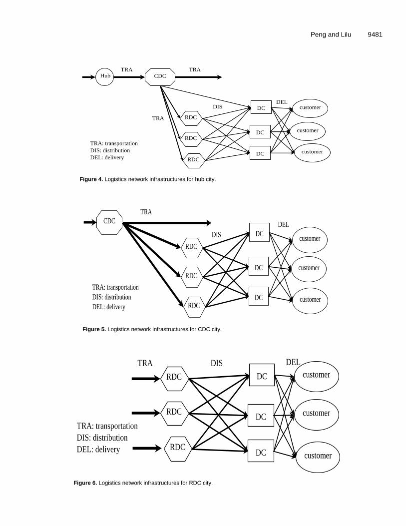
We define the PCA score as efficiency while DEA score as effectiveness of logistics infrastructures. The 31 regions of China are scattered in Figure 3. From Figure 3, we classify LNIs into four clusters, as shown in Figure 4. (1) Benchmark cluster: In this cluster, both PCA score and DEA score are high in the region (PCA score >= 0 and DEA score = 1), and the logistics infrastructures are both efficient and effective, within Guangdong Province, Jiangsu Province, Shandong Province, Shanghai Municipality, Hebei Province, Liaoning Province, Beijing Municipality, Inner Mongolia Autonomous Region and Fujian Province. (2) Efficiency cluster: In this cluster, PCA score is high but DEA score is low in the region (PCA score > = 0 and Developing policy for hub city In hub cities, four-tier logistics network is designed, in which goods is transported from the hub to the CDC, then distributed to RDC, finally reached DC and delivered to the customers as illustrated in Figure 5.

9476 Afr. J. Bus. Manage.

Table 1. Evaluation index system for LNIs.

First-grade factor Second-grade factor Indicator (unitage) Abbreviation

Inputs

The scale of logistics industry

Total investment Total Investment in Fixed Assets in the Transport, Storage and Post Industry (billion Yuan)

TIFA-TSP

Number of employed persons

Number of Employed Persons in Transport and Postal Services (thousand person)

NEP-TSP

Economic development level

Disposable income

Disposable Income of Urban Households (thousand Yuan per capita)

DIUH

Consumption expenditure Consumption Expenditure of Urban Households (thousand Yuan per capita)

CEUH

Industry developing level Number of State-owned and State-holding Enterprises (thousand unit) NSSE

Total Retail Sales Total Retail Sales of Consumer Goods (billion Yuan) TRSCG

Transportation accessibility

Railway accessibility

Railway Density (Km / thousand Km2)

RWD

Waterway accessibility Waterway Density (Km / thousand Km2) WWD

Highway accessibility Highway Density (Km / thousand Km2) HWD

Accessibility of trucks Possession of Civil Motor Vehicles (thousand unit) PCMV

Accessibility of vessels Possession of Civil Transport Vessels (thousand unit) PCTV

Outputs

Output of logistics industry

Capability of freight

Turnover Volume of Freight Traffic (billion ton-kilometers)

TVFT

Capability of GDP Gross Domestic Product in the Transport, Storage and Post Industry (billion Yuan)

GDP-TSP

Table 2. Synthetic scores of 31 regions of China (Year, 2009).

Region Indicator

I1 I2 I3 I4 I5 I6 I7a I8a I9a I10 I11 O1 O2

Beijing 66.25 273.49 26.74 17.89 6.89 530.99 71.44 0.00 1267.87 144.14 0.00 73.16 55.66

Tianjin 48.37 90.63 21.40 14.80 8.33 243.08 47.74 5.41 1233.50 72.90 0.24 960.66 47.10

Hebei 102.62 217.18 14.72 9.68 13.10 576.49 298.12 0.00 813.36 626.62 0.11 640.52 149.19

Shanxi 73.59 185.75 14.00 9.36 4.02 280.90 216.02 28.53 814.23 356.86 0.22 239.04 52.34

Inner Mongolia 78.64 143.72 15.85 12.37 4.47 285.53 493.23 146.78 131.65 245.69 0.00 411.69 77.33

Liaoning 75.76 269.87 15.76 12.32 23.36 581.26 258.36 25.23 696.11 460.51 0.72 775.39 79.06

Jilin 42.38 122.47 14.01 10.91 5.94 295.73 239.07 88.96 464.10 200.53 0.92 116.73 34.18

Heilongjiang 65.18 230.42 12.57 9.63 4.41 340.18 351.62 313.41 336.54 273.79 1.18 164.47 43.36

Shanghai 88.28 184.65 28.84 20.99 17.91 517.32 19.41 135.99 1850.78 162.97 1.91 1437.26 63.50

Jiangsu 102.02 259.16 20.55 13.15 60.82 1148.41 101.13 1479.76 1424.47 430.35 32.64 467.53 142.33

Zhejiang 100.87 184.97 24.61 16.68 59.97 862.23 102.52 592.74 1048.09 463.77 20.66 565.99 88.80

Peng and Lilu 9477

Table 2. cont’d

Anhui 46.01 117.65 14.09 10.23 14.12 352.78 174.09 341.83 1062.59 367.88 25.45 632.17 46.79

Fujian 88.54 127.43 19.58 13.45 18.15 448.10 128.88 198.25 734.28 185.50 2.43 247.13 75.14

Jiangxi 38.20 138.35 14.02 9.74 7.54 248.44 165.69 344.40 818.94 190.06 4.05 233.42 39.49

Shandong 103.25 270.29 17.81 12.01 45.52 1236.30 225.15 61.83 1477.58 670.76 5.68 1102.22 174.23

Henan 58.38 226.25 14.37 9.57 18.11 674.64 241.25 77.38 1463.25 717.97 4.63 615.40 82.36

Hubei 76.74 274.02 14.37 10.29 14.03 592.84 182.06 503.81 1059.27 262.40 4.18 256.64 64.27

Hunan 102.78 182.21 15.08 10.83 13.31 491.37 225.60 702.22 901.08 348.59 9.90 251.33 70.48

Guangdong 159.62 399.54 21.57 16.86 52.19 1489.18 151.41 723.50 1044.48 794.38 9.31 476.97 159.53

Guangxi 60.23 153.19 15.45 10.35 5.68 279.07 190.96 331.89 424.35 224.60 8.60 233.72 37.88

Hainan 18.64 39.09 13.75 10.09 0.49 53.75 23.66 20.96 589.81 39.01 0.51 79.25 8.87

Chongqing 64.34 111.64 15.75 12.14 6.41 247.90 80.49 264.60 1344.21 208.73 3.66 165.05 34.80

Sichuan 125.00 199.95 13.84 10.86 13.27 575.87 199.02 654.88 514.48 428.14 7.23 159.05 52.07

Guizhou 39.72 74.34 12.86 9.05 2.79 124.73 121.11 210.28 808.85 148.54 1.95 92.60 39.98

Yunnan 57.09 125.11 14.42 10.20 3.49 205.11 151.18 154.67 536.56 325.91 0.85 86.76 17.95

Tibet 8.24 6.67 13.54 9.03 0.09 15.66 32.10 0.00 44.70 15.25 0.00 3.53 2.12

Shaanxi 59.95 166.99 14.13 10.71 4.48 269.97 202.78 65.10 699.90 213.99 1.14 221.86 42.32

Gansu 15.50 86.11 11.93 8.89 1.99 118.30 148.77 55.82 281.51 122.43 0.50 161.95 21.36

Qinghai 12.41 27.45 12.69 8.79 0.52 30.05 102.44 20.13 84.04 50.51 0.07 36.42 4.93

Ningxia 9.01 26.18 14.02 10.28 0.97 33.93 54.37 7.14 420.52 85.30 0.57 75.04 11.48

Xinjiang 33.99 91.91 12.26 9.33 2.02 117.75 224.40 0.00 92.26 227.53 0.00 125.59 20.91

mean 65.21 161.51 16.28 11.63 14.01 428.00 168.52 243.73 789.79 292.44 4.82 358.34 59.35

standard deviation 35.81 89.14 4.33 2.98 17.16 357.85 102.22 320.81 465.26 202.63 7.86 342.74 44.67 a computed by Total Length of Highways divided by area of the region. Data in this table are from the Department of Service Survey, National Bureau of Statistics of China. Data on

transportation are from Ministry of Railway, Ministry of Transport, Civil Aviation Administration of China, China Petroleum and Natural Gas Corporation Group, China Petrochemical Corporation Group, the divisions of vehicle management under the provincial departments of public security, which are subordinate to the Traffic Management Bureau, Ministry of Public Security. Data on postal and telecommunication services come from the Ministry of Industry and Information, and the National Postal Office.

There is a relatively better operating system in Hub cities, that the focus of LNIs planning is on enhancing the improvement and integration of the logistics systematic function, strengthening the

mechanization, automatization and informationi-zation, improving the capacity of handling and efficiency of different logistics facilities, developing multimode transportation, facilitating efficient connection between facilities and transport line, and optimizing operation process for cost control.

In practice, advanced operation model should

be introduced, that is, synthetic logistics facility should be built to attract supplier of components, and integrated operation system with supply-produce-sale and quick response should be instructed. Developing Policy for CDC City In CDC cities, three-tier logistics network is designed, in which goods is transported from the

CDC to the RDC, then distributed to DC and delivered to the customers. In this system, larger RDCs should be built for outboard transportation, which should be located around the industry park with convenient transportation network with the surrounding areas, that is, goods and material can be distributed to the surrounding areas directly through this facility. And lager DC should be built for distributing goods to retails, stores, even the final consumers (see Figure 6).

For transportation network construction, it is the

9478 Afr. J. Bus. Manage.

Table 3. Eigenvalues of the correlation matrix (13 variables).

Component Initial Eigenvalues Extraction Sums of Squared Loadings

Total % of Variance Cumulative % Total % of Variance Cumulative %

1 7.031 54.082 54.082 7.031 54.082 54.082

2 2.262 17.399 71.481 2.262 17.399 71.481

3 1.545 11.883 83.365 1.545 11.883 83.365

4 0.726 5.582 88.947

5 0.476 3.663 92.610

6 0.366 2.814 95.424

7 0.190 1.465 96.889

8 0.152 1.168 98.056

9 0.126 0.968 99.025

10 0.060 0.465 99.490

11 0.034 0.258 99.747

12 0.022 0.168 99.916

13 0.011 0.084 100.000

Figure 3. Scree plot of eigenvalues.

long distance transportation system that should be con-structed with urban distribution network improvement as a supplement, that is, to construct a smooth outboard transportation system. Developing policy for RDC city In RDC cities, two-tier logistics network are designed, in

Table 4. Component loadings (Eigenvectors).

variables Component

PC1 PC2 PC3

TIFA-TSP 0.871 0.216 0.100

NEP-TSP 0.837 0.261 0.213

DIUH 0.653 -0.680 0.107 CEUH 0.639 -0.649 0.168 NSSE 0.900 0.013 -0.254 TRSCG 0.959 0.148 -0.011 RWD 0.074 0.790 0.391 WWD 0.602 0.184 -0.702 HWD 0.719 -0.428 0.076 PCMV 0.764 0.492 0.176 PCTV 0.583 0.055 -0.709 TVFT 0.634 -0.306 0.413 GDP-TSP 0.892 0.248 0.171

which goods is transported from RDC to DC, then delivered to the customers (See Figure 7). In this system, DCs should be built to enforce the capacity of small-size, multiple-item, and high-frequency order-picking, to improve the capacity of automatic handling, and to speed up the response. RDCs should also be built to accept the goods supplied by surrounding areas and distribute the goods to DCs timely.

Developing policy for the DC city

In DC cities, goods is transported directly to DC and delivered to the customers. For transportation network construction, it is the urban distribution network that

Peng and Lilu 9479

Table 5. Ranking of 31 regions of China on indicators of environment (using 13 variables).

Region PC1

Score

PC1

Ranking

PC2

Score

PC2

Ranking

PC3

Score

PC3

Ranking

GDP-TSP

GDP-TSP

Ranking

PCA

Score

PCA

Ranking

DEA

Score

DEA

Ranking Cluster

a Remark

Guangdong 5.680 1 -0.823 29 1.576 2 159.53 2 3.738 1 1 1 1

Benchmark

Jiangsu 4.383 2 1.830 1 1.826 1 142.33 4 3.486 2 1 1 1

Shandong 4.261 3 -1.420 31 -1.170 28 174.23 1 2.301 4 1 1 1

Shanghai 2.547 5 -0.753 27 -2.379 31 63.50 12 1.156 5 1 1 1

Hebei 1.795 6 -0.790 28 -0.082 18 149.19 3 0.988 6 1 1 1

Liaoning 1.495 8 -0.881 30 -0.555 25 79.06 7 0.707 10 1 1 1

Beijing 0.992 9 -0.538 26 0.091 15 55.66 13 0.544 11 1 1 1

Inner Mongolia 0.532 12 -0.089 15 0.666 6 77.33 8 0.422 13 1 1 1

Fujian 0.173 15 -0.356 22 0.517 9 75.14 9 0.112 15 1 1 1

Zhejiang 3.529 4 -0.494 24 0.994 4 88.80 5 2.328 3 0.877 20 2

Efficiency

Hunan 0.875 10 1.205 2 0.730 5 70.48 10 0.923 7 0.725 24 2

Sichuan 0.704 11 0.930 4 1.152 3 52.07 15 0.815 8 0.545 30 2

Henan 1.578 7 -0.495 25 -1.331 29 82.36 6 0.731 9 0.941 18 2

Hubei 0.529 13 0.856 5 0.050 16 64.27 11 0.529 12 0.805 21 2

Anhui 0.441 14 1.038 3 -0.587 27 46.79 17 0.419 14 0.898 19 2

Shanxi -0.501 18 0.016 12 -0.259 23 52.34 14 -0.359 18 1 1 3

Effectiveness

Tianjin -0.411 17 -0.481 23 -1.777 30 47.10 16 -0.620 21 1 1 3

Guizhou -2.202 25 0.318 9 -0.150 21 39.98 20 -1.383 25 1 1 3

Xinjiang -2.278 26 -0.261 20 0.272 10 20.91 26 -1.494 26 1 1 3

Gansu -2.800 27 -0.064 14 -0.078 17 21.36 25 -1.841 27 1 1 3

Hainan -3.321 28 -0.129 17 -0.354 24 8.87 29 -2.232 28 1 1 3

Ningxia -3.335 29 -0.337 21 -0.141 20 11.48 28 -2.254 29 1 1 3

Tibet -4.055 31 -0.203 19 0.256 11 2.12 31 -2.637 31 1 1 3

Heilongjiang -0.336 16 0.603 7 0.567 7 43.36 18 -0.011 16 0.642 27 4

Weakness

Guangxi -0.740 19 0.737 6 0.547 8 37.88 22 -0.248 17 0.608 29 4

Shaanxi -0.903 20 0.012 13 -0.170 22 42.32 19 -0.607 19 0.737 23 4

Chongqing -0.914 21 0.258 10 -0.563 26 34.80 23 -0.620 20 0.676 25 4

Jiangxi -1.260 22 0.552 8 -0.138 19 39.49 21 -0.722 22 0.756 22 4

Jilin -1.300 23 -0.166 18 0.133 14 34.18 24 -0.859 23 0.623 28 4

Yunnan -1.512 24 0.024 11 0.170 13 17.95 27 -0.952 24 0.388 31 4

Qinghai -3.647 30 -0.102 16 0.189 12 4.93 30 -2.360 30 0.670 26 4

Note: a cluster 1: PCA score >= 0 and DEA score = 1; cluster 2: PCA score >= 0 and DEA score < 1; cluster 3: PCA score < 0 and DEA score = 1; cluster 4: PCA score < 0

and DEA score < 1.

9480 Afr. J. Bus. Manage.

Table 6. CRS input-oriented DEA results.

DMU Efficiency Score Slacks

I1 I2 I3 I4 I5 I6 I7a I8

a I9

a I10 I11 O1 O2

Z0 S-(1) S-(2) S-(3) S-(4) S-(5) S-(6) S-(7) S-(8) S-(9) S-(10) S-(11) S+(1) S+(2)

Beijing 1 - - - - - - - - - - - - -

Tianjin 1 - - - - - - - - - - - - -

Hebei 1 - - - - - - - - - - - - -

Shanxi 1 - - - - - - - - - - - - -

Inner Mongolia 1 - - - - - - - - - - - - -

Liaoning 1 - - - - - - - - - - - - -

Jilin 0.623 - 22.278 3.037 2.877 - 39.551 70.634 46.929 - - 0.466 123.902 -

Heilongjiang 0.642 1.087 71.348 - 0.059 - 57.737 - 130.854 65.980 26.621 0.646 49.752 -

Shanghai 1 - - - - - - - - - - - - -

Jiangsu 1 - - - - - - - - - - - - -

Zhejiang 0.877 23.641 - 8.698 5.783 24.322 74.166 - 177.587 - 85.612 9.857 - -

Anhui 0.898 - 14.577 - 0.314 1.415 - 108.895 275.002 133.627 190.858 21.718 - -

Fujian 1 - - - - - - - - - - - - -

Jiangxi 0.756 - 42.922 4.076 2.946 0.200 - 59.173 256.700 228.134 - 2.748 70.014 -

Shandong 1 - - - - - - - - - - - - -

Henan 0.941 - 74.996 0.434 - - 131.653 90.919 44.512 556.974 366.261 2.526 - -

Hubei 0.805 2.510 115.673 - 0.309 - 152.426 - 263.991 390.031 - 1.185 - -

Hunan 0.725 14.158 21.290 - 0.338 - 35.884 - 423.478 202.496 - 6.053 36.983 -

Guangdong 1 - - - - - - - - - - - - -

Guangxi 0.608 5.596 31.860 2.999 1.763 - 18.879 - 181.032 - - 5.180 7.721 -

Hainan 1 - - - - - - - - - - - - -

Chongqing 0.676 13.668 8.888 1.421 1.923 - - - 177.460 395.435 34.786 2.394 189.668 -

Sichuan 0.545 31.930 32.688 2.295 2.442 2.684 112.569 - 354.757 - 15.464 3.897 65.519 -

Guizhou 1 - - - - - - - - - - - - -

Yunnan 0.388 5.409 14.903 0.500 0.266 - 8.432 - 39.251 - 56.262 0.148 - -

Tibet 1 - - - - - - - - - - - - -

Shaanxi 0.737 5.495 45.228 - 0.344 - 30.168 - - 114.917 - 0.543 - -

Gansu 1 - - - - - - - - - - - - -

Qinghai 0.670 2.793 8.003 6.727 4.557 - - 41.977 4.917 3.775 18.539 0.015 - -

Ningxia 1 - - - - - - - - - - - - -

Xinjiang 1 - - - - - - - - - - - - -

Mean 0.867 10.629 38.820 3.354 1.840 7.155 66.147 74.320 182.805 232.374 99.300 4.098 77.651 0.000

Peng and Lilu 9481

Hub CDC

DC

RDC

DCRDC

DC

TRA

RDC

customerDISDEL

customer

customer

TRA: transportation

DIS: distribution

DEL: delivery

TRA

TRA

Figure 4. Logistics network infrastructures for hub city.

DC

RDC

DCRDC

DCRDC

CDC

customerDIS

DEL

TRA: transportation

DIS: distribution

DEL: delivery

TRA

customer

customer

Figure 5. Logistics network infrastructures for CDC city.

DCRDC

DCRDC

DCRDC

customer

DIS DEL

TRA: transportation

DIS: distribution

DEL: delivery

TRA

customer

customer

Figure 6. Logistics network infrastructures for RDC city.

9482 Afr. J. Bus. Manage.

DC

DC

DC

customer

DEL

TRA: transportation

DIS: distribution

DEL: delivery

customer

customer

TRA

TRA

TRA

Figure 7. Logistics network infrastructures for DC city.

should be constructed by expansion of traffic road network and traffic capacity improvement, thus a distri-bution channel, in which the routing optimization within urban area is the focus, and long distance transportation is a supplement, should be set up based on urban GIS and freight characteristics.

Conclusions

31 sample regions' LNIs of China are classified into four clusters based on PCA-DEA method. We define the PCA score as efficiency and DEA score as effectiveness of logistics infrastructures, the 31 regions are classified into four clusters including benchmark cluster, effectiveness cluster, efficiency cluster and weakness cluster.

We found that China has nine benchmark cluster regions, six effectiveness cluster regions, eight efficiency cluster regions and eight weakness cluster regions of LNIs. The evaluation framework of LNIs is partly tested by empirical study and needs further and deeper research.

ACKNOWLEDGEMENT

The research is supported in part by Great Subject Research Project on Philosophy and Social Science of the Chinese ministration of education “Common Benefit Type Society Welfare Theory and System Construction in China” (Number: 10 JZD0033). REFERENCES Ali AI, Seiford LM (1993). The Mathematical Programming Approach to

Efficiency Analysis, In: Fried HO, Lovell CAK and Schmidt SS (Eds), The Measurement of Productive Efficiency, Oxford University Press, New York pp.120-159.

Banker RD, Charnes A, Cooper WW (1984). Some Models for Estimating Technical and Scale Inefficiencies in Data Envelopment Analysis. Manag. Sci. 30:1078-1092.

Boles JN (1966). Efficiency Squared – Efficient Computation of Efficiency Indexes, Proceedings of the 39th Annual Meeting of the Western Farm Economic Association pp.137-142.

Boussofiane A, Dyson RG, Thanassoulis E (1991). Applied data envelopment analysis. Eur. J. Oper. Res. 52:1-15.

Charnes A, Cooper W, Rhodes E (1980). The distribution of DMU efficiency measures. J. Enterp. Manag. 2(2):160-162.

Charnes A, Cooper WW, Lewin AY, Seiford LM (1995). Data Envelopment Analysis: Theory, Methodology and Applications, Kluwer. Springer; 1 edition (July 31, 1995).

Charnes A, Cooper WW, Rhodes E (1978). Measuring the Efficiency of Decision Making Units. Eur. J. Oper. Res. 2:429-444.

Debreu G (1951). The Coefficient of Resource Utilization. Econometrica 19(3):273-292.

Farrell MJ (1957). The Measurement of Productive Efficiency. J. R. Statis. Soc. 120(3):11-48.

Koopmans TC (1951). An Analysis of Production as an Efficient Combination of Activities. In: Koopmans (ed.), Activity Analysis of Production and Allocation. Cowles Commission for Research in Economics, Monograph 13. New York: John Wiley and Sons, Inc.

Lovell CAK (1993). Production Frontiers and Productive Efficiency. In: Fried HO, Lovell CAK and Schmidt SS (Eds), The Measurement of Productive Efficiency, Oxford University Press, New York pp.3-67.

Lovell CAK (1994). Linear Programming Approaches to the Measurement and Analysis of Productive Efficiency. Top 2:175-248.

Lu C-s, Yang C (2006). Evaluating key logistics capabilities for international distribution center operators in Taiwan. Trans. J. 45(4):9-27.

Mentzer K (1991). An efficiency/ effectiveness approach to logistics performance analysis. J. Bus. Logis. 12(1):33-61.

Seiford LM (1996). Data Envelopment Analysis: The Evolution of the State of the Art (1978-1995). J. Prod. Anal. 7:99-138.

Seiford LM, Thrall RM (1990). Recent Developments in DEA: The mathematical Approach to Frontier Analysis. J. Econometrics 46:7-38.

Shephard RW (1953). Cost and Production Functions.Princeton: Princeton University Press.

Zhang X (2004). Research on the theory of the location planning for logistics park. Beijing: China Logistics Publising House Press.