a study of auctioneer’s decisions

Université de Montréal

Wine Auctioning:

A Study of Auctioneer’s Decisions

Présenté par:Arnaud Franco

Département des sciences économiques

Faculté des arts et des sciences

Rapport de recherche présenté à la Faculté des études supérieures

en vue de l'obtention du grade de

Maîtrise èn sciences (M.Sc.) en Sciences Économiques

Mai 2006

i

Abstract

Auction houses across the world must decide in which way to organize the lots which

they sell in their auctions. This paper examines the decisions faced by a wine auctioneer

whose goal is to obtain the highest price per bottle for the wines she is selling. Data from

the USA’s Chicago Wine Company were used in order to answer two specific questions

which deal with lot formation.

Initially the study focuses on lots which only contain one particular vintage in varying

quantities (single-vintage lots), and then considers the case of lots with multiple vintages

in varying quantities (multi-vintage lots). The study notes that when taking into account

the particular characteristics of the wines in question (such as the quality, the place of

origin, and the physical bottle condition), the results and subsequent conclusions maybe

be different than when simply considering price averages.

Using both ordinary least squares and maximum likelihood regressions, the study’s

first conclusion is that, contrary to a result obtained by Bentzen and Smith (2003),

increasing the number of bottles in a single-vintage lot will decrease the overall price per

bottle of that lot, when all the wine’s characteristics are taken into account. The second

result was the identification of a positive link between the size of a multi-vintage lot and

its valuation. More specifically, the study shows that as the size of the multi-vintage lot

increases, so does the probability that the bottles in the lot will cost less per bottle than if

ii

they were bought individually. Both results combine together to show that if an

auctioneer wishes to obtain the maximum price per bottle for her lots, she should sell

each of her wines individually as single unit lots.

iii

Sommaire

Les maisons d’enchères partout dans le monde doivent décider dans quelle façon

organiser les lots qu’elles mettent en vente. Ce rapport examine les décisions qui font

face à une maison d’enchères qui a le but d’obtenir le prix maximum par bouteille de vin

qu’elle met en enchère. Des données du Chicago Wine Company sont utilisées pour

répondre à plusieurs questions qui concernent la formation des lots.

Initialement l’étude se base sur les lots qui contiennent seulement une cuvée

particulaire et puis considère après les lots qui contiennent plusieurs cuvées différentes.

L’étude note que quand les caractéristiques particulaires des vins (comme sa qualité, son

origine, et la condition de sa bouteille) son contrôlés, les résultats et conclusions peuvent

être différentes qu’une étude qui considère seulement les moyennes.

En se servant des régressions moindres carrées ordinaires et maximum de

vraisemblance, l’étude réussi à établir un lien positive et significatif entre la quantité

vendu et le prix par bouteille payé. La conclusion finale est donc qu’une maison

d’enchères qui cherche à maximiser son prix par bouteille est mieux de vendre ses vins

en lots individuelles.

iv

“In Vino Veritas”“In wine there is truth”

“Bonum vinum laetificat cor hominis”“Good wine gladdens a person’s heart”

v

Table of Contents

Abstract........................................................................................................... i

Sommaire ...................................................................................................... iii

I. Introduction ........................................................................................ 1

II. The Auction ......................................................................................... 6

III. Past Research .................................................................................... 14

IV. The Data ............................................................................................ 18

V. The Quantity-Price Ratio Model..................................................... 28

VI. The Multi-vintage Model ................................................................. 41

VII. Conclusion ......................................................................................... 51

Annex ........................................................................................................... 53

Bibliography ................................................................................................ 62

vi

List of Tables

Table 1: Bidding increments of the Chicago Wine Company auction ........ 12

Table 2: Summary of important variables for single-vintage lots ............... 25

Table 3: Summary of important variables for multi-vintage lots ................ 26

Table 4: Average prices per bottle of three selected Bordeaux wines per lot size ................................................................................................................ 28

Table 5: Regression output of log-level model............................................ 31

Table 6: Regression output of log-level model with interaction terms ....... 38

Table 7: Probit regression output of multi-vintage model........................... 44

Table 8: OLS regression output of multi-vintage model ............................. 48

Table I: Greater and Sub-Region Wine Production Statistics..................... 59

Table II: Sub-Region production as a percentage of Entire Bordeaux Production ..................................................................................................... 60

Table III: Summary of Sub-region dummies .............................................. 61

vii

List of Figures

Figure 1: Average prices per bottle of three selected Bordeaux wines according to lot size ...................................................................................... 53

Figure 2: Wine producing region of Bordeaux in France............................ 54

Figure 3: Wine bottle dimensions................................................................ 55

Figure 4: Greater Region Production in Bordeaux...................................... 56

Figure 5: Sub-Region Production in Médoc Greater Region ...................... 56

Figure 6: Sub-Region Production in Graves Greater Region ...................... 57

Figure 7: Sub-Region Production in Rivers Greater Region....................... 57

Figure 8: Sub-Region Production in Côtes Greater Region ........................ 58

1

I. Introduction

Since the beginning of modern wine production (heralded by Baron Edmond de

Rothschild in 1870)1 the wine industry has greatly evolved from its origins of producing a

sweet and unappealing beverage to catering to the intellectual and health-savvy obsession

of many individuals in many countries across the world. The world demand for wine has

risen steadily over the recent years, having grown by nearly 2% (in volume) in 2003 to

25,066 million litres2 (with the market for red wine responsible for most this growth). In

the period from 1997 to 2003, the total world consumption of wine increased by 6.9%.3

This increase in demand can be attributed in part to the modern scientific studies

which claim that the polyphenol substances found in red wine reduce the risks of many

common health hazards such as heart disease, cancer, strokes, and even Alzheimer’s

disease.4 Wine is also becoming a more and more sophisticated hobby and the increase in

demand has been highlighted by an increase in better quality products, especially in

Western Europe, Scandinavia, the United States and Australia. This could be explained in

part by an increase in disposable income and living standards in the countries concerned.

New wine markets in countries like China (having grown by 58% between 1996 and

1 Jewish Virtual Library (http://www.jewishvirtuallibrary.org)

2 Euromonitor International (http://www.euromonitor.com)

3 The Wine Institute (http://www.wineinstitute.org)

4 Professional Friends of Wine (http://www.winepros.org)

2

2001),5 Russia, and South Korea (from 1993 to 1996, Korean wine imports nearly tripled,

increasing from $5.9 million to $16.5 million)6 have also contributed significantly to the

increased demand. New players in the wine production market such as South Africa and

New Zealand have also contributed to an increasing world interest for this beverage. It is

interesting to see however, that in certain Western European countries like France and

Spain, consumers seemed to have moved away from the traditional every-day

consumption of wine to a more occasional consumption (marked by a declining demand

of 2.5% in the period of 2003).

In the United States, there has been a steady increase in demand, and it is estimated

that the wine market contributed nearly 45$ billion to the US economy in 2003, as well as

creating 556,000 jobs. It is estimated that wineries have grown at a rate of 14%, leaving

most states with over 25 wine producing companies,7 even though just over 50% of the

American wineries are located in California.

The increased sophistication of wine has also increased the instances of consumers

searching for rare and generally unavailable wines. This is where we see the growing role

of wine auctioning in the expansion of the wine market. Wine auctions range from small,

country-style wine fairs to immense and sometimes charity wine auctioning events. One

of the largest American wine auctioning companies is the Napa Valley Auctions

5 Research and Markets (http://www.researchandmarkets.com)

6 USDA Foreign Agricultural Service (http://www.fas.usda.gov)

7 Bloomington @ Work (http://www.journalism.indiana.edu/gallery/j201fall03/Bloomington@Work/KatieFinal)

3

Company. This company has organized the largest charity event in the United States: the

Auction Napa Valley. Since its conception in 1981, this event has raised 62$ million for

charity. In its more commercial auction, Premiere Napa Valley, the company has

estimated a 28% increase in their revenues from the 2006 auction (vis-à-vis the 2005

auction).8 Now with the Internet, everyday consumers can view and participate in various

wine auctions on a multitude of online auction sites from their own home. Although these

websites have grown at a rate to complement the dot-com boom of the 21st century, the

caliber of most sites is not as impressive as traditional in-person auctions; the largest and

most prestigious auction sales still occur in the traditional fashion.

The goal of this paper is to answer certain questions which become even more

relevant with the growing demand for wine auctioning. The questions asked in this study

will focus on the decisions which a wine auctioneer faces in deciding the makeup of the

lots she wishes to auction off.

In this paper, an auction is defined as a method of selling property in a public forum

through open and competitive bidding. The word auction however will be used to denote

the entire process in which lots are sold in an entire day. In other words, the combination

of each individual lot sold constitutes an auction.

The first issue focuses on the quantity-price ratio of wine sales. More specifically, is

it more profitable to sell wines by the bottle or in lots of several bottles (two bottles or a

crate of six, twelve, or twenty-four)? Although according to certain economic theories, a 8 Napa Valley Wineries (http://www.napavintners.com/auctions/premierenv.html)

4

sale in bulk would lower the price paid per bottle,9 this is not necessarily true. Many

factors such as the order of the lots or the amount of a particular vintage sold in one day

can influence consumer’s willingness to pay as the auction runs its course. We can also

hypothesize that the quality and rarity of the wine may cause an increase in its price per

bottle. Wine lots which contain only one vintage in varying quantities will be referred to

as a single-vintage lot.

The second issue deals with the profitability for the auction house to group different

wines together, creating a multi-vintage lot. For example, could an auctioneer manage to

increase the price per bottle by grouping a lower quality wine with a higher quality wine

in a single lot? Would this increased price be higher than the price she would have

received had she sold the wines individually? We will examine the profitability of these

so called multi-vintage lots.

In the following sections, I will attempt to answer the above questions using an

auction structure for which I have obtained raw live data. Section II will give a brief

theoretical summary of the three most common auction types (English, Vickerey, and

Dutch) and then focus on describing the auction of the Chicago Wine Company. Section

III presents past studies published about the wine auctioning market. Section IV

examines the data obtained from the Chicago Wine Company and their manipulation. In

Section V we will examine the price-quantity relationship for single-vintage lots by

comparing study of averages to an ordinary least squares regression which takes into

9 This is an example of second degree price discrimination.

5

account the particular characteristics of the wines. Section VI examines the multi-vintage

issue using a probit model and a simple ordinary least squares regression. And finally,

section VII presents the final observations and conclusions of the study.

6

II. The Auction

Many wine auctioning companies use different procedures, each of which offer a

variety of incentives for consumers and producers to do business with them. Each

company will set its terms and conditions to appeal to a certain base-type of consumers.

The framework we will analyze in this paper will be the auction structure used by the

Chicago Wine Company (“the Company”) in their monthly auctioning system. In this

system, the Company receives consignments of varying quantities of bottles from

individual or corporate sellers. The Company decides to group the bottles in various

different lot formats (single bottle, multi-bottle or multi-vintage) and determines the order

in which they will be sold during the course of the entire auction. This paper attempts to

examine the profitability of these decisions.

In its formulation, the Company applies the English auction model. The English

auction is a first-price, ascending-bid auction in which bidding continues until no bidder

will go higher than the bid proposed by the auctioneer. The rules for an English auction

are simple and the system has been used for over centuries by some of England’s oldest

auction houses like Sotheby’s, Christie’s, and Phillips to provide the most efficient

auctioning system for both the auctioneer and the consumers and producers.

As we can expect, the auction system begins from a low bid set by the auctioneer and

increases in increments specified by the auctioneer, until no participant is willing to bid

7

higher than the highest bid registered. When the bidding stops, the item or lot is said to be

‘hammered down’ or ‘knocked down’ and the price at which this occurs is said to be the

‘hammer price’. It is often assumed that when an item has been hammered down, it has

been sold to the highest bidder, but this is not necessarily true.

This is because before the auction takes place, the seller of the item or the auction

house may set a ‘reserve price’. This reserve price is a minimum price which the seller

accepts to sell the item. Therefore an item or lot which is hammered down before the

reservation price is reached is unsold and is said to have been ‘bid in’. In wine

auctioning, it has been observed by Ashenfelter (1989) that about 5 to 10 percent of lots

are ‘bid in’.

During an auction, every item will be treated, bid on, and knocked down as if it had

been sold. It is only after the auction, upon collection of the item, that a buyer will know

if the item or lot she was bidding on has been ‘bid in’. Thus, an auctioneer will never

reveal the reservation price of an item or lot, as it would cause buyers to attempt to buy

only just above this price to draw the maximum surplus away from the seller. When an

item is bid in, the seller must wait a certain time before attempting to sell the item once

again. It has been stated by Ashenfelter (1989) that the repeated auctioning of a certain

item or lot may cause its future value to diminish. When this occurs, an item is said to

have been ‘burned’.10

10 Ashenfelter. How auctions Work for Wine and Art

8

It is a common misconception that the auctioneer will begin the bidding at the reserve

price. The auctioneer will generally start the bid at a level she deems reasonable, and this

is generally (by contract) left entirely to her discretion. Another misconception about the

power of the auctioneer is that she can, usually at the end of the sale of an item or lot,

invent fictitious bids to extract the maximum from the buyers (as stated by Graham and

Marshall (1987)). This is not only unethical, but also quite illegal and since the rules of

the auctioneer are available to the public, such behavior would not be tolerated long.

Since an auction houses most important asset is its reputation, no well-known auction

house would engage in such practices. The auction business is an example of an industry

where the reputation of an auction house can serve as a significant barrier to entry to

competitors.

Of equal importance but often ignored in economic literature, is the role of the

auctioneer in the auction process. The auctioneer is the dominant party in the process, and

is the key which makes the auction engine run. In a perfectly rational economic structure,

the auctioneer would play no role whatsoever. Buyers would all pay their willingness’s to

pay and sellers would set their reserve price to obtain their desired profit.

However, reality suggests otherwise. The job of the auctioneer is to draw the buyers

into the game, to extract the highest valuation from them, but at the same time to allow

the customers to feel relaxed so as to feel like they have gotten a fair deal. Many

consumers believe that the auctioneer acts on behalf of the seller, but this is not

9

necessarily true. Since the auctioneer receives compensation from both the buyer and the

seller, it can be said that she acts in her own best interest.

A buyer’s premium (implemented by most auctions) is a sum charged to the buyer of

an item or lot to act as commission to the company selling the good (usually a fixed

percentage). A buyer’s premium causes the willingness to pay of a consumer to be

diminished as the consumer has the knowledge that the final price she will be paying is

not the price she bids11.

The seller’s commission is a sum charged by the auction house to sell the good (also

usually a percentage). Generally the size of this seller’s commission is not fixed, and is

negotiable based on the relationship between the seller and the auctioneer and the size of

the consignment (the total amount of wine a seller wishes to sell).

According to Ashenfelter (1989), in the recent years, the auction business has

progressed such that auction houses experience greater profits manipulating the buyer’s

premiums rather than seller’s commissions due to the fact that they usually deal with

large consigners who can bargain down the seller’s commission. This is not necessarily

the case. Since a large buyer’s premium can reduce the willingness to pay of a consumer

it may thus increase the chance of a lot being ‘bid in’. A good or lot which has been ‘bid

in’ brings neither a premium nor commission to the auctioneer. Therefore, to make sure

the auction house still profits from bid in items, there is usually a fee for unsold goods,

generally expressed as a percentage of the reserve price. This is an important strategic 11 Townsend Real Estate (http://www.townsend-real-estate.com/Buyers_Premium.htm)

10

consideration when setting the reserve price. This is logical as making the fee a function

of the reserve price will cause sellers to risk less by setting a lower reserve price, causing

the item or lot to be more likely to sell.

The English auction is not the only commonly used auction system. We will briefly

examine two other auction systems which are also used in wine and art auctioning: the

Vickerey auction and the Dutch auction.

The Vickerey auction is a non ascending secret bid auction in which all bidders write

their bids on ballots which are collected by the auctioneer. The auctioneer then examines

the bids and the winner is chosen to be the bidder who bid the most. The Vickerey

auction is also known as a second-price auction because the winner of the lot will only

pay the second highest bid. In this auction, as demonstrated by to the Nobel Prize

winning economist William Vickerey, the Nash equilibrium results when the bidders bid

their true willingness to pay, knowing that they will only end up paying the second

highest bid. All bidders thus have a dominant strategy to bid their willingness to pay.

Another common type of auction is the Dutch auction. This auction is called a

descending price auction as the starting bid usually starts at quite a high level. The

auctioneer then decreases the price gradually until a bidder tells him to stop. This bidder

will then win the lot and pay the price at which the auctioneer stopped. Dutch auctions

are usually characterized by the speed of the auction process, and are very common in

bulk flower auctions.

11

The Company auction is similar to the English auction described previously, with a

few specifications and refinements. All of the lots to be auctioned off are advertised in a

free catalogue which can be ordered prior to the auction. The Company reserves the right

to withdraw any lot prior to or during the auction for whatever reason. Anyone above the

age of 21 can register with the Company prior to the auction if they wish to participate in

the live bid. Absentee bids may be placed by mail, e-mail, telephone, or fax, before the

auction. These bids will be executed by the Company at or below a specified price, and

the Company is not held liable for the failure to place any of these bids or any other

errors relating to the execution of such bids. This stated, an absentee bidder can request

that the Company limit her overall expenditures in the auction to a pre-determined limit.

If this request is made, the Company will cease bidding on all lots once the absentee

bidder reaches the predetermined limit. All bidding in the live auction is done with

paddles only. The highest bidder acknowledged by the auctioneer will be the winner of

the lot. The auctioneer holds the authority to reject any bid and to advance the bidding. In

the event of an argument between bidders, the auctioneer reserves the right to determine

the successful bidder or to resell the item in dispute. For all arguments which follow the

auction, the final sale shall be the winner as determined by the Company auctioneer. All

bidding will be done in accordance with the bidding increments published by the

Company in its catalogues prior to the auction. The increments are as follows.

12

Table 1: Bidding increments of the Chicago Wine Company auction

Range Increment Example

$10 $200 $10 $110, $120, $130$200 $1,000 $20 $220, $240, $260$1,000 $2,000 $50 $1050, $1100, $1150$2,000 $5,000 $100 $2100, $2200, $2300$5,000 $10,000 $200 $5200, $5400, $5600Over $10000 $500 $10500, $11000, $11500

Source: The Chicago Wine Company: Terms and Conditions (www.tcwc.com/terms.htm)

The auctioneer reserves the right to change the bidding increments at any time.

The hammer price of a lot will be the purchase price. The Company does not charge a

buyer’s premium. In actual fact, the Company is the only large live auction house in the

United States which does not have a buyer’s premium. Although a lot may reach a final

selling price, a seller or the auctioneer may, as stated earlier, implement a reserve during

the course of the entire auction (not the single lot auction). All charges such as the

relevant sales taxes and other charges which the Company is required by law to collect

will be imposed on the hammer price of the lot. This being stated, the Federal Excise Tax

(currently of 18 cents per 750 ml bottle) is absorbed by the Company and will not be

charged to the buyer. No lots are to be taken away or shipped until the auction has ended

and until the purchase price has been paid in full. All shipments made by the Company

must be in accordance to the laws of the origin and destination involved. Many states in

the USA have laws to regulate the flow of alcoholic beverages. The Company agrees to

13

assist with any shipping request made by the buyers, with the understanding that all

arrangements are made by the buyer himself and thus all plaints for damages are to be

made to the shipping company and not the Company. All auctions sold by the Company

are sold as is, and thus no warranties of any nature exist. The Company also charges no

lotting and no lot collection fees, which are costs to the seller and buyer respectively,

which accompany selling and buying a lot. In addition the Company does not charge an

automatic 1% insurance rate which many auctioning companies will require.12

As for the seller, The Company charges a 28% seller’s commission. Thus, of the

hammer price of the lot, The Company receives 28% and the consigner receives 72%

(after the respective taxes and duties stated in the terms and conditions are accounted

for). For example, if a lot were to sell for $200, The Company would receive $56 and the

consigner would receive $144 (ignoring the taxes and duties). This percentage is

negotiable and may vary depending on the size of the consignment a particular seller

wishes to sell and the relationship which exists between The Company and the consigner.

12 The Chicago Wine Company (www.tcwc.com)

14

III. Past Research

In this section, I will examine other studies which have been conducted on wine

auctioning and wine prices to build the scene for my analysis. Although not much

research has been done in the field of wine auctioning, two studies were chosen which

will allow us to examine certain findings of other economists and their implications on

the global state of the wine auctioning market. Two studies will be examined; the first

dealing with the concerns of consumer information in wine auctions and how personal

consumer characteristics affect reserve prices. The second study deals with price

evolution in US, Danish and international markets, and the effect of business cycle

indicators on the latter.

The first paper examined is a study written by Lecocq, Magnac, Pichery and Visser

(2003) which consists of a simulated experiment in which individuals endowed with

varying degrees of information were randomly placed in three separate rooms and

informed about the characteristics and quality of certain wines. The participants were

then given the chance to evaluate the wines which were sequentially auctioned off in four

separate Vickerey auctions.

The authors then examined certain personal characteristics of the individuals and

attempted to draw conclusions about how these characteristics affected their behavior and

more importantly their willingness to pay. This article yielded interesting conclusions.

15

The authors noticed that certain socio-economic characteristics such as gender, income,

and consumption habits affected significantly a person’s willingness to pay, and others

such as age and nationality played no role. Also, varying the type of information that

individuals disposed of showed some interesting results. The authors found that when

participants who entered the experiment had prior knowledge of the quality and

characteristics of the wine to be evaluated, tasting the wine had no effect whatsoever in

changing their willingness to pay.

They also found that if participants who had no prior knowledge tasted the wines

blindly and were advised by an expert who informed them of the characteristics and

opinions of the wines in question, their willingness to pay increased dramatically. This

leads to an interesting conclusion which shows that even if a participant has never tasted

the wine in question, the opinion of a “professional”, be it a wine guide or an expert,

would be sufficient in increasing their willingness to pay. Information made available

from “professionals” is thus more reliable than personal perceptions and opinions of the

blind tasting.

The explanation of the authors is the following: a wine can be assumed to be a bundle

of characteristics and attributes. These attributes can be divided into two groups, search

and experience or sensory attributes. Search attributes can be evaluated by a consumer by

examining the label or consulting a wine guide or expert, where as the sensory

characteristics can only be obtained through tasting the wine. Assuming that none of the

participants in the experiment were experts, we can assume that the sensory attributes are

16

difficult to observe by the agents and thus it would be difficult for them to observe the

actual quality of the wine. The best technique for the agents to gain a good knowledge of

the wine quality is by listening to the experts and the guides, and therefore to suppress

their experience perceptions of the wine.

Search attributes thus preside over sensory attributes in explaining the willingness to

pay.

In a paper published by Bentzen and Smith (2003), their focus lay in the comparison

and evolution of the price of a particular wine, the Mouton Rothschild premier cru classé,

a Bordeaux wine from the region of Pauillac. The paper begins by gathering data on the

price of the Mouton Rothschild (1982) from several auction houses worldwide and

comparing them to attempt to study the price difference across countries. Next the

authors attempt to find a link between the prices of these wines and certain business cycle

indicators.

The first interesting result of this paper comes when the authors examine data

provided to them by the Chicago Wine Company and find that the average price per

bottle of the Mouton Rothschild 1982 actually increases as the size of the lot increases.

They hypothesize that this trend could be in part due to the fact that large lots are more

professionally stored than individual bottles. Also they state that in many cases, the large

lots are sold in their original wood cases. I conducted a very similar study on three

different wines, the Chateau Mouton Rothschild 1998, the Chateau Lafite Rothschild

17

1998 and the Chateau Latour 1995, and obtained similar conclusions as Bentzen and

Smith. These results will be exhibited in Section V (See Table 4).

The paper continues to compare the price of the wine in the USA, Denmark, England

and the rest of the world. The authors note that prices seem to vary quite dramatically

across countries. This effect could be attributed in part to the fact that fine wines, such as

the wine studied, are in less demand in Denmark than in the United States. This affect

could also be attributed to the varying taxes which apply to the sale of alcohols in the

respective countries.

The main goal of the paper was to compare certain business cycle indicators to the

international price of the icon wine and to attempt to find a link between the two. The

conclusion of this analysis was that even when a broad range of economic indicators were

used, no significant link was found between the movements of the Mouton Rothschild

1982 and the movements of these indicators.

The study was particularly interesting due to its similarity with the questions asked in

this paper. Both the price per bottle and financial indicators analysis coincide with

aspects which this paper will examine. Moreover, the primary source of data for Bentzen

and Smith was the Chicago Wine Company, which is the source of the results to be

shown later. Our studies differ however, in the respect that I focus on the decisions made

by the auctioneer in determining the final price whereas Bentzen and Smith examined

only the final sale prices.

18

IV. The Data

The data used in this paper is obtained from the Chicago Wine Company auctions.

These nearly monthly auctions were recorded, and the hammer prices, lot numbers, and

wine quantities, sizes, and descriptions were all noted. I use data from auction number

329 on January 28, 2004 to auction number 343 on December 21, 2004 (11 auctions in

total: there was none in the month of October). Each observation in the data corresponds

to one specific lot, be it a single-vintage or a multi-vintage lot. This being said, certain

characteristics of single-vintage lots are not applicable to multi-vintage lots and vice

versa. The data set was compiled to include only French Bordeaux red wines, even

though The Company holds auctions for many different wines. The decision to only

observe red wines from this region was made to obtain a homogenous data set of wines.

The wines varied amongst a set of specific characteristics such as quality, year, and

physical condition (explained later). This amounted to 10,425 individual lots sold. After a

brief analysis, it was noted that 13.36% of the lots sold consisted of single unit lots or

more specifically, lots which only contained one bottle of wine.

Since the modern ages of wine production, the Bordeaux region in France has been

one of the most prestigious wine-producing regions in the world. From its vineyards have

come some of the highest quality and most valued wines along with a history and

tradition of excellence. In 2003, the Bordeaux region’s 57 appellations and roughly 7,000

19

chateau’s produced 779.3 million bottles of wine,13 accounting for 25% of the high

quality wine production in France.14 We can consider that the Bordeaux region can

generally be divided geographically into four wine-producing regions. Within these

regions, fifteen sub-regions15 have been distinguished (Figure 2 in the annex shows all

the Bordeaux regions, not just the ones which appeared in the data) as the quality and

characteristics of a wine will most certainly vary across the regions of Bordeaux.

The largest of these greater-regions is the Rivers region, which includes the massive

Bordeaux Supèrieur sub-region, which spreads over 51400 hectares. In its entirety, the

Bordeaux Supèrieur sub-region produced nearly 62% of the entire Bordeaux wine

product (475 million bottles) in 2003 (see Table II in annex). Although this area is by far

the largest sub-region, we find very little mention of it in the data set observed. This is

largely due to the fact that the wines produced from this region are not as high quality as

the wines produced in the other sub-regions. Probably the most common greater-region in

our sample would be the Côtes region. This area (which accounts for only 13.43% of the

Bordeaux production) contains the very prestigious Pomerol and St. Emilion sub-regions.

As we shall see later, the majority of the wines in our data sample originate from this

greater-region (see Table III in annex). The smallest greater-region, Graves, is fairly

present in the data, mostly because of wines from the Pessac-Lèognan sub-region, which

13 Total includes both red and white wines

14 In this case “high quality” is used to describe AOC (Appellation Origine Controlée) appellations. These appellations are considered by wine experts as the highest quality wine producers in the country. Terroir-France (http://www.terroir-france.com)

15 It is important to note that more than 15 sub-regions exist (21 actually) in the Bordeaux area, but only 15 were specified because only wines from these 15 sub-regions were found present in the Chicago Wine Company data.

20

produces several fine wines. It is interesting to note that the sub-region of Sauternes in

the Graves area is a region which produces only sweet white wines. There are therefore

no observations in our data originating from this region. The last greater-region is the

region of Médoc. This area is common in the data as well, but perhaps not as common as

the Côtes area. The greater-region of Médoc contains many of the finest French wineries,

including those from the Pauillac sub-region. Throughout the world, Pauillac is

considered as one of the sub-regions in which the best Bordeaux wines are produced (See

Figures 4-8 and Tables I and II in annex for additional details).

To account for this specification of sub-regions, dummy variables were created for

each lot which categorized the place of origin of the particular wine. As stated earlier, the

Bordeaux sector was divided into fifteen individual sub-regions. Fourteen dummy

variables were thus generated, one sub-region being excluded to act as the zero-condition

region (the sub-region of Bordeaux Supérieur). Since multi-vintage lots can contain

bottles of wine from different regions, these regional dummies are not employed in their

case. Different binary variables were thus generated to exhibit the decisions made by the

auctioneer to group the wines together in a multi-vintage format. The first variable

specifies if the wines in the multi-vintage lot are of the same year, the second specifies if

the wines are produced by the same chateau, and the third specifies if the wines are from

the same region in the Bordeaux sector.

The data set was also trimmed to include only bottles of the classic 0.75 liter size. All

other bottles of magnum size or higher (including double magnums, imperials,

21

jeroboams, and salmanazars; see Figure 3 in annex) were removed from the sample. This

decision was made to ensure the stability of the quantity variable, allowing it to vary per

observation based on the assumption that all the bottles were of the same size.

For example a lot of two 0.75 liter bottles is not necessarily equal to a lot of a single

magnum-sized bottle as the individual bottles can be consumed at different times, thus

increasing their value to the personal consumer. This may cause magnum-sized bottles to

be less expensive due the lack of demand. On the other hand, magnum and larger size

bottles are often purchased for prestigious events as they must be consumed entirely in

one session, and thus may sometimes be more valued for their rarity.

Next, a quality of wines variable was also employed. This variable was not generated

from the data obtained from the Company, but was drawn from the extremely well

known Parker wine ratings (www.erobertparker.com). These ratings are renowned and

are considered the top wine ranking benchmark in the world. The wines were rated on a

scale from 0 to 100, judged professionally by their taste, odor and color. Since the data

sample consists of lots that are both single-vintage and multi-vintage, this variable will

only be used in its raw form in the single-vintage case. In the multi-vintage case, the

quality is expressed as the average quality of all of the bottles in the lot.

An age variable was then generated using the year the wine was produced. This age

variable was calculated by setting the base year to 2003, since the newest wines sold in

22

the auctions (which were held in 2004) were from this year. In the multi-vintage case,

this variable is not used.

The next variables generated were order variables which rank the lots observed in the

order in which they were auctioned off during the day of a particular auction. This is

important to see if the price of a lot depended on whether it was sold earlier or later in the

auction. This variable is simply expressed as a number where the first lot auctioned off

takes value one and so on. In other words, the order variable resets for every auction (the

auction being the full day). This variable was generated independently for single-vintage

lots and multi-vintage lots. This being said, the order variable in the single-vintage case

represents the order in which the single-vintage lots were sold during the course of an

auction. The same applies for the multi-vintage order variable.

Another similar variable generated is a global order variable. This parameter is

similar to the first order variable except that it does not reset per auction. Thus, the global

order variable is simply a numerical progression which indicates the chronological order

in which the lots were sold over the period of a year, throughout all eleven auctions. This

variable is found only to be significant in the multi-vintage case; therefore it is not

present in single-vintage observations.

Similar to this, another variable was generated to state the amount of bottles of the

particular wine (same year and vintage) which was sold on that day. This variable

suggests that the sale of many bottles of a particularly good wine in a single auction could

23

have detrimental effects on its price. Since buyers at the auction have perfect knowledge

of all the wines to be auctioned off on a given day, a large supply of a particular wine

may cause its price for that day to fall. This variable was only used in the single-vintage

case.

The next variables generated are dummy variables which serve to explain the

condition of the physical bottles of wine. These variables were all manually generated

based on a description of each lot provided by The Company. Since many wines are

stored in humid cellars and are often left for long periods unmonitored it is not

uncommon that the physical bottle or the wine itself maybe be damaged. Damage to the

wine label, the cap, the cork, or sometimes even the bottle itself can have a detrimental

effect on the final price paid by consumers.

The following eleven discreet variables describe physical effects (mostly presumed to

be detrimental) to the bottle or the wine in question. These physical effects could affect

the willingness to pay of the consumer. A label-damage conditional was generated to

show that bottles with varying degrees of damaged labels are worth less per bottle than

undamaged bottles. The value of this variable ranged from 0 to 3, taking the value 3 when

the label was most damaged, and the value 0 when the label was in good condition. A

variable was also created to take into account if a bottle had its label replaced. Next, three

cork binary variables were created to show the position of the cork (depressed or raised)

and if the bottle has been re-corked. The next three variables, also binary, deal with the

condition of the cap on the wine (whether the cap is corroded, nicked, or even if there is

24

no cap at all). Another variable deals with the shoulder fill or level of wine in the bottle.

The level generally varies based on a combination of the age of the wine and the storage

conditions in which the wine was kept. A wine with a low shoulder fill is often a mark of

very poor storage and can be in many cases, undrinkable. Conversely, a high shoulder fill

is a good fill level for bottles which are more than 25 years of age. A mid shoulder fill

can be an indicator of poor storage and can result in a bottle being undrinkable, although

this fill level is common in wines which are more than 40 years of age. These details are

very important to keep in mind when purchasing old wines. This qualitative variable has

a value range of 1 to -2, taking the value -2 when the bottle in question shows a low fill,

and the value 1 when a bottle shows a high fill. When the variable is of value 0, the bottle

is of normal fill. The next variable accounts for the presence of sediment in a wine.

Sediment is often considered an indication of poor storage or unprofessional wine

fermentation, yet this is usually false. Sediment is often the result of natural wine aging,

and can, in many cases, be considered a good sign. It can also result from a wine not

being filtered before being bottled. Sediment is not harmful in any ways, and can be

removed by simply decanting the wine before consuming it. The final conditional

variable is binary and deals with the presence of a Balthus label. In the early 1990’s the

Mouton Rothschild wine producing estate hired an artist by the name of Balthus to design

the label of the 1993 wine and produce a series labels for different vintages. After having

been distributed, these labels were removed from the market for their slightly revealing

images which included mild nudity. Because of the rarity, these bottles are sought after

by wine collectors.

25

Since these physical effects can arise in only particular bottles in a crate (say one

bottle in a crate of twelve is damaged) a method to account for this had to be

implemented. The value of these discreet variables equaled the average of the

corresponding dummy variable for each of the bottles in the lot. For example, if a crate of

twelve bottles contained two bottles with sediment, then the sediment dummy would

have a value of 0.167. In the case of multi-vintage lots, these binary variables are not

employed. This is due to the fact that examination of the data showed that all the bottles

included in multi-vintage lots were in pristine condition and had none of the particular

traits listed above. These variables are thus only considered in the single-vintage case.

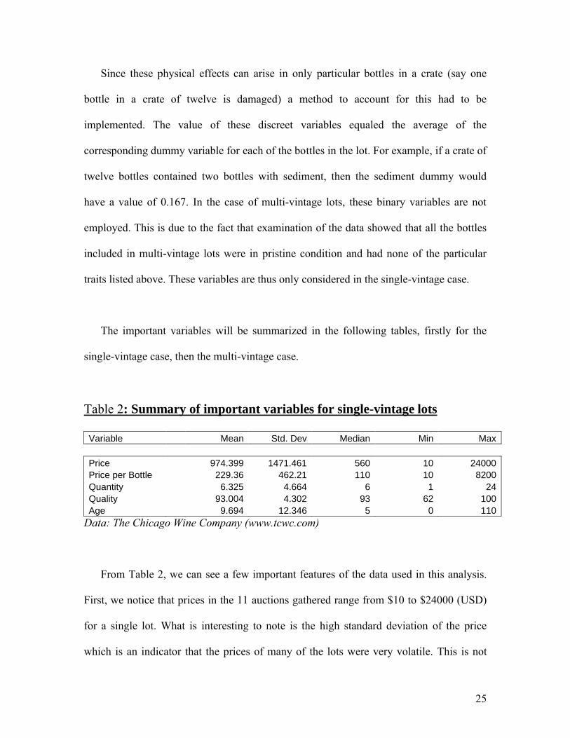
The important variables will be summarized in the following tables, firstly for the

single-vintage case, then the multi-vintage case.

Table 2: Summary of important variables for single-vintage lots

Variable Mean Std. Dev Median Min Max

Price 974.399 1471.461 560 10 24000Price per Bottle 229.36 462.21 110 10 8200Quantity 6.325 4.664 6 1 24Quality 93.004 4.302 93 62 100Age 9.694 12.346 5 0 110

Data: The Chicago Wine Company (www.tcwc.com)

From Table 2, we can see a few important features of the data used in this analysis.

First, we notice that prices in the 11 auctions gathered range from $10 to $24000 (USD)

for a single lot. What is interesting to note is the high standard deviation of the price

which is an indicator that the prices of many of the lots were very volatile. This is not

26

surprising as lots varied in size from single bottle lots to crates of 24 (as we can see from

the quantity variable). The average of the quantity variable shows us that the average lot

sold consisted of roughly six bottles of wine and the average price of these lots were of

$974.4. We can see from average price variable that the average price paid by buyers per

bottle was of $229.36. These prices for individual bottles ranged from $10 to $8200. We

can see a fairly high standard deviation, which exhibits a similar high variation we saw in

the price per lot. The Quality variable ranges from 62 to 100, which serves to show that

the wines studied ranged from mediocre quality wines to wines of very high quality. The

average quality of 93 combined with the average price per bottle for the wines from the

Bordeaux region is a very good indicator of the overall quality of the wines produced in

this region, which are truly among the best in the world. We can also see the age variable

ranges from 0 to 110. This indicates to us that the sample’s oldest wine dates back to

1893, and the newest wines are from 2003. The mean age of the wines is roughly 10,

which means wines from 1993. This as well as a fairly high variance, indicates to us that

there exist outliers in the lower boundary which must be dealt with.

Table 3: Summary of important variables for multi-vintage lots

Variable Mean Std. Dev Median Min Max

Lot Price 295.369 464.060 180 30 4600Lot Value 353.265 483.979 240 60 4035Quantity 3.943 2.927 3 2 23High Value 129.391 164.992 90 20 1600Low Value 61.783 30.343 60 20 150High Quality 90.787 3.847 91 80 100Low Quality 85.631 5.955 86.5 50 95Same Year 0.631 0.484 1 0 1Same Chateau 0.123 0.330 0 0 1Same Region 0.336 0.474 0 0 1


27

From the above summary, we can point out a few interesting characteristics of the

data. Firstly we can see the high standard deviation associated with prices, as mentioned

before. The lot price variable describes the price paid for a multi-vintage lot, and the lot

value variable shows the compiled value of that lot. This value is calculated by finding

the prices that a buyer could have paid had she bought the individual bottles at the same

auction, rather than the multi-vintage lot. It is extremely important to note that since all

the bottles sold in multi-vintage lots were in pristine condition (they exhibited no sign of

the conditional variables described earlier), the value variable is drawn from identical

bottles, or more specifically, pristine bottles. This thus explains why no conditional

variables are use in the multi-vintage case. The average price of a multi-vintage lot was

of $295. Conversely, the average value of a multi-vintage lot was of $353. This shows us

that, on average, multi-vintage lots were under valued. The median statistic supports this

result. The Quantity variable here tells us that the average number of bottles in a multi-

vintage lot was roughly 4. The final 3 variables show us the decisions made by the

auction house in creating multi-vintage lot. According to the data, 61% of the multi-

vintage lots contained bottles of the same year, 12% contained bottles from the same

chateau, and 33% contained bottles from the same region.

28

V. The Quantity-Price Ratio Model

Before an econometric analysis was run on the data gathered, a short study on price

per bottle of three specific Bordeaux wines was carried out. This analysis was conducted

in the attempt to show that comparing averages can yield different conclusions than a

more specific study which takes into account the characteristics of the wines. These three

wines, the Chateau Mouton Rothschild 1998, the Chateau Lafite Rothschild 1998, and the

Chateau Latour 1995, were chosen because of the fact that they are wines that sell in

varied quantities (from one bottle to a case of 24) due to their popularity. These three

wines are also wines of very similar quality (96, 98, and 96 respectively). Table 4 shows

the variation in the price per bottle according to the size of the lot.

Table 4: Average prices per bottle of three selected Bordeaux wines per lot size


Average price per bottleLot size

Ch. Mouton Rothschild 1998 Ch. Lafite Rothschild 1998 Ch. Latour 1995

1 120 156.67 2202 150.63 168.18 255.834 154.62 169.62 258.936 152.22 160 266.67

12 155.95 169.91 260.4224 155.9 175 291.67

29

Table 4 shows a tendency towards increasing price per bottle with respect to lot size

(see Figure 1 in annex for graphical results). This result shows us that when averages are

concerned, the price per bottle will be greater as the lot size increases.

This exhibits the same conclusions as the study conducted by Bentzen and Smith

(2003). They conclude that this result is explainable by the fact that large lots are, on

average, stored more professionally than small lots or single bottles, and are thus more

desirable.16 We can also hypothesize that there exists a transaction cost (time spent at the

auction) in the purchase of many individual lots versus the purchase of one single large

lot.

The goal of this study is to attempt show that if we only consider the averages and not

the particular characteristics of the wine, we may obtain erroneous conclusions.

An Econometric model was then specified to see if, when the particular

characteristics of the wines are taken into account, we obtain the same result exhibited in

the average study conducted above. The estimation of the model was done using an

ordinary least squares regression with a log-level framework. Examination of the data

confirmed the presence of quite a few large important outliers which needed to be

accommodated for. The log of the price per bottle was thus used to account for these

outliers.

16

Bentzen and Smith. A Comparative Study of Wine Auction Prices: Mouton Rothschild Premier Cru Classé

30

Log(priceperbottle) = α0 + α1quantity + α2order + α3numsold + α4quality + α5lnage +

β + ΓC +

Where is the vector of regional dummies and C is a vector of discreet condition

variables, and α1 represents the semi-elasticity of price per bottle with respect to

quantity.17

The following presents the results of the previous model. Two separate regressions

are presented, one using the main framework described above, and the other including

two interaction terms between important variables which lead to slightly different

conclusions.

When the original regressions were constructed, a Breusch-Pagan test for

heteroskedasticity was conducted on each. The null hypothesis of homoskedasticity was

rejected in both, thus confirming the presence of heteroskedasticity. To account for this,

the regressions were both conducted using heteroskedastic robust standard errors.

17 In actual fact, in a log-level model, the semi-elasticity is denoted as 100*α1 as it shows the % change in price per bottle with respect to a change in quantity.

31

Table 5: Regression output of log-level model

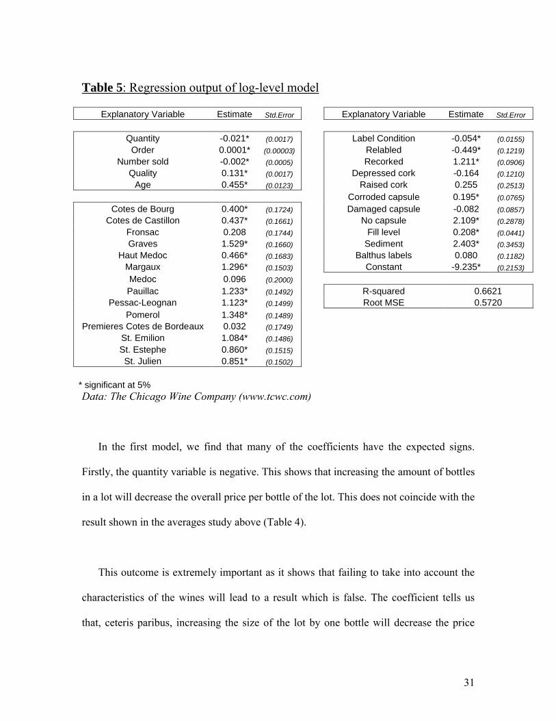
Explanatory Variable Estimate Std.Error Explanatory Variable Estimate Std.Error

Quantity -0.021* (0.0017) Label Condition -0.054* (0.0155)

Order 0.0001* (0.00003) Relabled -0.449* (0.1219)

Number sold -0.002* (0.0005) Recorked 1.211* (0.0906)

Quality 0.131* (0.0017) Depressed cork -0.164 (0.1210)

Age 0.455* (0.0123) Raised cork 0.255 (0.2513)

Corroded capsule 0.195* (0.0765)

Cotes de Bourg 0.400* (0.1724) Damaged capsule -0.082 (0.0857)

Cotes de Castillon 0.437* (0.1661) No capsule 2.109* (0.2878)

Fronsac 0.208 (0.1744) Fill level 0.208* (0.0441)

Graves 1.529* (0.1660) Sediment 2.403* (0.3453)

Haut Medoc 0.466* (0.1683) Balthus labels 0.080 (0.1182)

Margaux 1.296* (0.1503) Constant -9.235* (0.2153)

Medoc 0.096 (0.2000)

Pauillac 1.233* (0.1492) R-squared 0.6621Pessac-Leognan 1.123* (0.1499) Root MSE 0.5720

Pomerol 1.348* (0.1489)

Premieres Cotes de Bordeaux 0.032 (0.1749)

St. Emilion 1.084* (0.1486)

St. Estephe 0.860* (0.1515)

St. Julien 0.851* (0.1502)

* significant at 5%Data: The Chicago Wine Company (www.tcwc.com)

In the first model, we find that many of the coefficients have the expected signs.

Firstly, the quantity variable is negative. This shows that increasing the amount of bottles

in a lot will decrease the overall price per bottle of the lot. This does not coincide with the

result shown in the averages study above (Table 4).

This outcome is extremely important as it shows that failing to take into account the

characteristics of the wines will lead to a result which is false. The coefficient tells us

that, ceteris paribus, increasing the size of the lot by one bottle will decrease the price

32

paid per bottle in that lot by 2.1%.18 Although this result is statistically significant, its

economic significance is better explained when examining the price per bottle in large

lots rather than in small lots.

All other things equal, increasing a 6 bottle lot to a 12 bottle lot would decrease the

price per bottle by 12.6%. Similarly, increasing a 12 bottle lot to a 24 bottle lot would

decrease the price per bottle by 25.2%. In other words, if a 12 bottle lot was priced at

$1200 ($100 per bottle), adding 12 bottles of the same wine to the lot would cause the lot

price to be $1795.20 ($74.8 per bottle), all other things remaining equal. A brief

experiment (results not shown here) was conducted to attempt to establish a non-linear

link between the price per bottle and the quantity. The results showed that there existed

no such non-linear link.

The expected sign of the order variable is not necessarily clear. One could expect that

the later in the auction that the lot was sold, the less the seller would obtain per bottle.

However this is not always the case. The order variable is positive, which is

explainable by the fact that in the Chicago Wine Company auctions, the more expensive

lots are sold at the end of an auction. This would mean that, other factors remaining

constant, the price per bottle of any lot would be higher if it was sold at the end of an

auction.

18 Calculated using: %y = 100*1x

33

The sign of the total number sold variable, however, is expected and clear. The

coefficient states that for every bottle of a particular vintage and year sold on the given

day of an auction, the price paid per bottle of that wine decreases by 0.2%. This result

shows that if there is a large supply of a particular wine on a particular day, the

consumers will pay less per bottle.

The quality variable is another variable whose coefficient bears the expected sign. It

states that, each unit of quality increases the price per bottle of a wine by 13.1%. For

example, if we were to compare two wines, one of quality 80 and the other of 100, (all

other factors remaining equal) the second wine would, cost roughly twice as much (262%

more) per bottle than the first.

It was noted above that the age variable was susceptible to outliers due to its low

average but quite high maximum value. For this purpose, the age variable was used in log

form to take into account these outliers. Its coefficient also has the expected sign, stating

that the more a wine has aged, the greater the price paid per bottle, ceteris paribus.

In a separate regression (not shown here), an attempt was made to find the existence

of a non-linear relationship between price per bottle and age. This could show that as

wines pass their prime drinkable age, their price per bottle increases by less than before.

This effect could not be identified. This is possibly explainable by the fact that wines past

their prime can still retain their value as collector’s items, rather than a drinkable product.

34

The variables that follow are the regional binaries. Their values yield very simple

conclusions. The region which was set as being the zero condition is the region of

Bordeaux Supérieur, thus the magnitudes of the dummy variables simply state whether

wines from the given region cost more or less per bottle than wines from the Bordeaux

Supérieur region, all else being equal. For example, the data set tells us that a wine from

the region of Pauillac would cost 75% more per bottle than a wine with the exact same

characteristics from the Bordeaux Supérieur. We can see that all of the regional dummies

are positive since wines from the Bordeaux Supérieur are lower priced, and only three are

not significant at the 5% level.

The next variables to be analyzed are the collection of discreet conditional variables.

Although many of the coefficients of these variables show the expected signs, a few go

against what could be expected.

The label damage conditional shows a negative coefficient, which explains that

bottles with varying degrees of damaged labels are worth less per bottle than undamaged

bottles. This is the expected sign. The coefficient tells us that, ceteris paribus, a bottle of

wine with a very slightly damaged label will have its price per bottle reduced by 5.4%.

Similarly, a bottle with a slightly more damaged label will be worth 10.8% less per bottle

and a wine bottle with a very damaged label will be worth 16.2% less. The Relabeled

variable, also negative, tells us that a wine bottle which has been relabeled is worth 45%

less per bottle, all other things remaining equal.

35

The three cork conditional variables bear varied conclusions. Although the depressed

and raised cork variables are insignificant, they bear the expected signs. The surprising

result is that the coefficient of the variable which deals with a re-corked wine is positive

and significant. This would mean that re-corking a wine would increase its value per

bottle versus exact non re-corked bottles (by 121% per bottle), ceteris paribus.

Of the next three variables which deal with the condition of the cap on the wine, two

yield positive coefficients, which is not expected. Two of these variables, the corroded

cap and the no cap variables are significant at the 5% level. A possible explanation for

this is that upon analysis of the data, it seems that capsule damage occurs only in

expensive and high quality wines. Since the price of these is fairly volatile and their

appearance on the auction market can be rare, buyers may tend to overlook a damaged

capsule or the fact that a capsule is missing when placing their bids on the wine(s).

The sign of the coefficient of the shoulder fill variable is as expected, and it is

significant at a 5% level. As explained earlier, the fill variable ranged from 1 to -2,

equaling 1 if the bottles exhibited a high shoulder fill, 0 if the fill was normal, -1 if the fill

was medium shoulder, and -2 if the fill was low. The coefficient indicates that a bottle

with low shoulder fill is worth 41.6% less per bottle than an exactly similar bottle with a

normal shoulder fill. Similarly, a bottle with a mid shoulder fill is worth 20.8% less per

bottle. Conversely, we can see that, ceteris paribus, a bottle with a high shoulder fill will

cost 20.8% more per bottle. This result is important as it distinguishes that there is a real

36

price difference between aged wines which have been well stored and wines which have

been poorly maintained.

Another variable which yields an expected and logical sign is the variable which

indicates the presence of sediment in the wines. The variable is significant at the 5% level

and its magnitude shows that a wine with sediment is worth 240% more per bottle than a

wine without sediment, all other things held constant.

The Balthus binary included in the regression yields a positive coefficient, which is

insignificant at the 5% level.

Finally, the interpretation of the constant is simple. The constant, which is significant

at the 5% level, can be described as the price of a wine which exhibits none of the

physical characteristics stated above and which originates from the region of Bordeaux

Supérieur and which was produced in the base year, 2003.

The first model overall shows a strong R2 of 0.66 which confirms a good overall

significance of variables.

The previous regression successfully showed that if we take into considerations the

particular characteristics of the wines being sold, that we would obtain a different

conclusion that the averages study conducted at the beginning of this section. It was

found that increasing the amount of bottles sold in a lot decreased the price per bottle of

37

that lot by 2.1%, all other factors held constant. A study was then conducted adding four

interaction terms in between quantity, quality and age. The reasoning for this was the

hypothesis that the semi-elasticity of the price per bottle with respect to these three

variables could depend on partial effects which they have on each other.

The new regressions in specified as:

Log(priceperbottle) = α0 + α1quantity + α2order + α3numsold + α4quality + α5lnage +

β + ΓC + 1quantity*quality + 2quantity*age + 3quality*age +

4quantity*quality*age +

The addition of interaction terms cause independent variables to affect the model in

different ways. It is important to distinguish between the two impacts which an

explanatory variable will have on the dependant variable when interaction terms are

added to the regression. Firstly we have the main effect. This effect is often considered

the direct effect of the dependant variable, regardless of the interaction terms. This effect

is better referred to as the constituent effect, as a main effect would imply that the

variables which have interaction terms are interpretable alone, which they are not. The

second effect is the interaction effect. This is described as the effect of a factor averaged

over another factor. The total effect is denoted as the sum of the constituent and

interaction effects.

38

Table 6: Regression output of log-level model with interaction terms


Quantity -0.755* (0.0360) Label Condition -0.054* (0.0145)

Order -0.0002* (0.00003) Re-labeled 0.642* (0.1196)

Number sold -0.0011 (0.0005) Re-corked -0.465* (0.1057)

Quality 0.119* (0.0026) Depressed cork -0.168 (0.1119)

Age -0.087* (0.0228) Raised cork -0.114 (0.2328)

Corroded capsule 0.166* (0.0709)

Cotes de Bourg 0.507* (0.1594) Damaged capsule -0.234* (0.0797)

Cotes de Castillon 0.418* (0.1537) No capsule 1.049* (0.2682)

Fronsac 0.392* (0.1616) Fill level 0.182* (0.0408)

Graves 1.126* (0.1554) Sediment 1.220* (0.3212)

Haut Medoc 0.521* (0.1557) Balthus labels 0.252* (0.1094)

Margaux 1.146* (0.1390) Constant -7.275* (0.2765)

Medoc 0.189 (0.1850)

Pauillac 1.139* (0.1381) Quantity * Quality 0.008* (0.0003)

Pessac-Leognan 1.025* (0.1387) Quantity * Age 0.060* (0.0027)

Pomerol 1.326* (0.1377) Quality * Age 0.0004* (0.00001)

Premieres Cotes de Bordeaux 0.105 (0.1620) Quantity * Quality * Age -0.0006* (0.00003)

St. Emilion 0.999* (0.1375)

St. Estephe 0.805* (0.1401) R-squared 0.7114St. Julien 0.774* (0.1390) Root MSE 0.5288


We find that the addition of these four interaction terms (quantity * quality, quantity *

age, quality * age and quantity * quality * age) alters the model slightly. The first and

most noticeable change is the increase (in absolute terms) in the magnitude of the

quantity variable. Secondly, we can notice a change in sign of the age variable. Besides

these two changes (which will be analyzed shortly), most of the coefficients have similar

values and significances. Surprisingly enough, the quality variable is not affected by the

addition of the interaction terms. This is curious because generally, there is at least a

small amount of interaction effects between variables. Since all the interaction terms are

found to be significant at the 5% level, they all affect the model in a real sense.

39

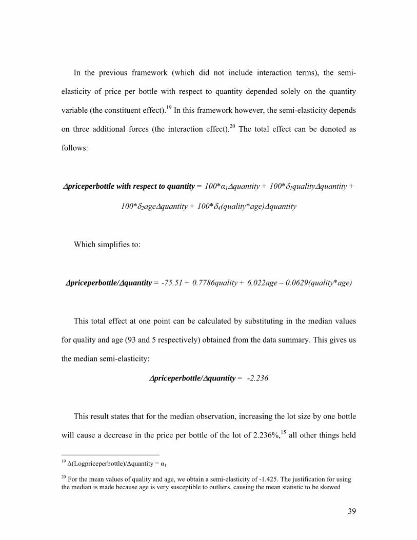
In the previous framework (which did not include interaction terms), the semi-

elasticity of price per bottle with respect to quantity depended solely on the quantity

variable (the constituent effect).19 In this framework however, the semi-elasticity depends

on three additional forces (the interaction effect).20 The total effect can be denoted as

follows:

priceperbottle with respect to quantity = 100*α1quantity + 100*1qualityquantity +

100*2agequantity + 100*4(quality*age)quantity

Which simplifies to:

priceperbottle/quantity = -75.51 + 0.7786quality + 6.022age – 0.0629(quality*age)

This total effect at one point can be calculated by substituting in the median values

for quality and age (93 and 5 respectively) obtained from the data summary. This gives us

the median semi-elasticity:

priceperbottle/quantity = -2.236

This result states that for the median observation, increasing the lot size by one bottle

will cause a decrease in the price per bottle of the lot of 2.236%,15 all other things held

19 (Logpriceperbottle)/quantity = α1

20 For the mean values of quality and age, we obtain a semi-elasticity of -1.425. The justification for using the median is made because age is very susceptible to outliers, causing the mean statistic to be skewed

40

constant. This result is not much different than the 2.1% found in the model with no

interaction terms.

We can speculate as to which of the two models is more appropriate. Critics of

interaction term models state that high levels of collinearity can arise, causing the

estimates to be distorted.21 The interaction term model exhibits a slightly larger R2

statistic of 0.71 and a smaller mean squared error statistic, making it a more likely choice,

regardless of the collinearity speculation. In essence however, both models have the same

results and conclusions.

21 http://www.ruf.rice.edu/~branton/interaction/faqfund.htm

41

VI. The Multi-vintage Model

When a wine auctioneer decides to sell her wines, she decides how to organize her

goods to obtain the maximum profit. In any given auction, and particularly in The

Company auctions, bottles can be sold in a variety of ways. We have seen from the

previous section that the auctioneer can sell a bottle individually or in groups of 2 to 24.

This section will instead deal with the decision of the auctioneer to create multi-vintage

lots instead of single-vintage ones.

A multi-vintage lot is a lot which consists of two or more wines with distinguishable

characteristics. This could include wines of different regions, or the same wines of

different years. One of these lots would be auctioned off and receive an individual price

for all the bottles in the lot. The auctioneer could make the decision to pair a high quality

wine with a weaker one to increase the total price paid for the lot. Conversely, this

decision may cause a decrease in the desire for the high quality wine.

The following study examines the profitability to the auctioneer of implementing a

multi-vintage lot. To do this, we will first calculate a variable (which will serve as our

dependant variable) to explain the success or failure of a seller to obtain more or less

from her multi-vintage lot than she would have obtained had she sold the bottles of the lot

individually. Since both multi-vintage and single-vintage lots are sold during the same

time period, it is always possible for a buyer to purchase the individual bottles separately,

42

instead of purchasing a multi-vintage lot. Doing this, she loses the certainty of obtaining

the particular bottles she wants individually. The data set was trimmed to include only the

multi-vintage lots which contained bottles which were individually available at the same

auctions the lots were being sold. This left a data sample of 122 observations.

We can state that an auctioneer has profited if her multi-vintage lot sells for more

than it would have sold if the bottles had been sold individually. This can be calculated

by individually computing the overall value of the lot using average wine prices complied

from the data, and comparing this overall value with the actual price the consumer paid

for the lot. As was mentioned earlier in section IV, this value was calculated using bottles

of the exact same condition (they were all pristine) as the ones included in the multi-

vintage lots.

It is important to note that although it may seem pointless to compare the total

“value” of a lot to the price actually paid (since in the auction system, a person pays her

willingness to pay and therefore her value for it is equal to what she paid), we view the

so-called compiled value more as the overall monetary worth of the lot rather than its

utility to the buyer.

If the consumer paid more than the overall compiled value, then she could have been

better off buying the wines individually at the same auction. In this case we say that the

lot was over valued. If, on the other hand, the overall compiled value of the lot was

greater than the price the consumer paid for the lot, then we say that the lot was under

43

valued, and the consumer is better off buying the multi-vintage lot than the individual

bottles. This over valuation or under valuation was calculated as a percentage and will

serve as the dependant variable of our study.

The following study examines all the multi-vintage lots which were auctioned off by

the Company in the eleven auctions used. The analysis examines two different angles of

the multi-vintage valuation starting with a probit regression which indicates which factors

cause the lot to be either over valued or under valued. The second will consider an

ordinary least squares regression which will explain to which degree certain factors affect

the percentage of over valuation or under valuation.

The probit model is specified as:

Over valued = 1Order + 2Global Order + 3Lot Price + 4Quanity + High Price +

6Low Price + 7High Quality + 8Low Quality + 9Var(Quality) + 1Same Year +

2Same Chateau + 3Same Region +

Where over valued is a binary variable which is equal to 1 when a lot is over valued

and 0 when a lot is under valued.

44

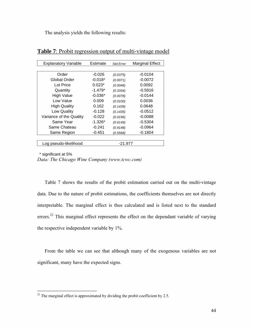
The analysis yields the following results:

Table 7: Probit regression output of multi-vintage model

Explanatory Variable Estimate Std.Error Marginal Effect

Order -0.026 (0.0375) -0.0104Global Order -0.018* (0.0071) -0.0072

Lot Price 0.023* (0.0046) 0.0092Quantity -1.479* (0.3334) -0.5916

High Value -0.036* (0.0078) -0.0144Low Value 0.009 (0.0100) 0.0036

High Quality 0.162 (0.1439) 0.0648Low Quality -0.128 (0.1435) -0.0512

Variance of the Quality -0.022 (0.0196) -0.0088Same Year -1.326* (0.6149) -0.5304

Same Chateau -0.241 (0.9148) -0.0964Same Region -0.451 (0.5568) -0.1804

Log pseudo-likelihood -21.977


Table 7 shows the results of the probit estimation carried out on the multi-vintage

data. Due to the nature of probit estimations, the coefficients themselves are not directly

interpretable. The marginal effect is thus calculated and is listed next to the standard

errors.22 This marginal effect represents the effect on the dependant variable of varying

the respective independent variable by 1%.

From the table we can see that although many of the exogenous variables are not

significant, many have the expected signs.

22 The marginal effect is approximated by dividing the probit coefficient by 2.5.

45

The order variable is negative and not significant at the 5% level. It states that as the

auction progresses, a multi-vintage lot’s chance of being under valued increases. In other

words, a multi-vintage lot sold near the end of an auction has a higher chance of being

under valued than a lot sold at the beginning of the auction, all other things equal.

Similar to this is the global order variable, which turns out to be significant at the 5%

level. Also negative, the global order variable tells us that as the year progresses, (the

2003 year consisted of 11 auctions) multi-vintage lots have a higher chance of being

under valued, ceteris paribus. For example, if a lot were the 100th multi-vintage lot to be

auctioned of during the course of the year, the chance that this lot would be under valued

increases by 72%.

The lot price variable has a positive sign, which is expected, and is statistically

significant. This states that the more a buyer paid for a particular lot, the higher the

change that the lot would be over valued. This is consistent as the lot price and lot value

are calculated independently and over valuation occurs when lot price is greater than lot

value. The marginal effect tells us that increasing the lot price by 1$ would increase the

chance of a lot to be over valued by 0.92%.

The quantity variable has a negative sign, which is an interesting result, and is

significant at the 5% level. This negative coefficient states that increasing the number of

bottles in a multi-vintage lot by one would lead to an increase in the chance of that lot

being under valued by 59%. This result is interesting as it resembles the result previously

46

obtained for single-vintage lots. Previously in section V, we found that increasing the

amount of the bottles in a single-vintage lot brought about a decrease in the price per

bottle of that lot, ceteris paribus. The above conclusion about multi-vintage lots tells us

that as we increase the number of bottles in a lot, we also increase the chance of under

valuation, all other factors being held equal. Since under valuation occurs when the price

paid is less than the compiled value, and the value is constant over all quantities, then we

can infer that increasing the quantity of bottles in a multi-vintage lot causes the overall

price per bottle of the lot to fall, causing under valuation.

The high value variable shows the expected sign and is significant. The low value

however is positive, which is curious, but is insignificant. We would expect that both of

these variables would be negative, stating that an increase in the maximum and minimum

values of the multi-vintage lot would cause an increase in the percentage of under

valuation, ceteris paribus.

The three quality-related variables are insignificant. The high quality variable is

positive, which could hint towards the possibility of a direct relationship between quality

and over valuation. The low quality variable, however, is negative which stands against

this possible conclusion. This states that increasing the maximum quality of a multi-

vintage lot by one point will increase the chance that this lot is over valued by roughly

6.5%. Conversely, increasing the minimum quality of the multi-vintage lot by one point

would decrease the chance that a lot would be over valued. This result could hint that

47

higher quality bottles are more subject to being over valued whilst lower quality bottles

are more subject to being under valued.

The final three variables are the binaries which deal with multi-vintage lot

composition. Of the three, only the binary which specifies that the bottles in the lot were

all produced in the same year is significant. Its coefficient tells us that having a multi-

vintage lot of bottles from the same year increases the chance of under valuation of the

lot by 53%. The other two binaries, the ones that specify that a lot comprises of bottles

from identical chateaus and identical regions, are also negative, despite being

insignificant.

Whilst the previous probit model shows which factors cause a multi-vintage lot to be

over or under valued, it does not examine the effect on the actual percentage of over or

under valuation. The following ordinary least squares model will focus on this

percentage, or in other words, the degree of over or under valuation.

% over valuation = 1Order + 2Global Order + 3Lot Price + 4Lot Value +

5Quanity + 6High Price + 7Low Price + 8High Quality + 9Low Quality +

10Var(Quality) + 1Same Year + 2Same Chateau + 3Same Region +

Where the % over valuation is positive in the case of an over valued lot and negative

in the case of an under valued lot.

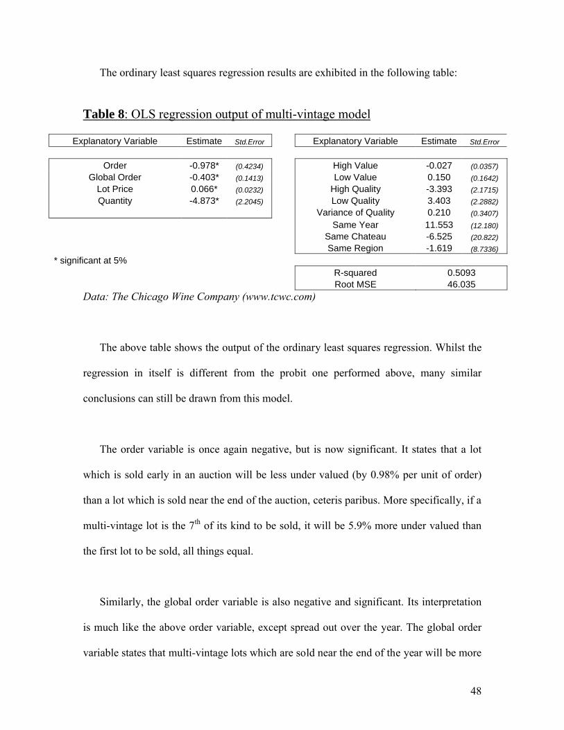
48

The ordinary least squares regression results are exhibited in the following table:

Table 8: OLS regression output of multi-vintage model


Order -0.978* (0.4234) High Value -0.027 (0.0357)

Global Order -0.403* (0.1413) Low Value 0.150 (0.1642)

Lot Price 0.066* (0.0232) High Quality -3.393 (2.1715)

Quantity -4.873* (2.2045) Low Quality 3.403 (2.2882)

Variance of Quality 0.210 (0.3407)

Same Year 11.553 (12.180)

Same Chateau -6.525 (20.822)

Same Region -1.619 (8.7336)

* significant at 5%R-squared 0.5093Root MSE 46.035


The above table shows the output of the ordinary least squares regression. Whilst the

regression in itself is different from the probit one performed above, many similar

conclusions can still be drawn from this model.

The order variable is once again negative, but is now significant. It states that a lot

which is sold early in an auction will be less under valued (by 0.98% per unit of order)

than a lot which is sold near the end of the auction, ceteris paribus. More specifically, if a

multi-vintage lot is the 7th of its kind to be sold, it will be 5.9% more under valued than

the first lot to be sold, all things equal.

Similarly, the global order variable is also negative and significant. Its interpretation

is much like the above order variable, except spread out over the year. The global order

variable states that multi-vintage lots which are sold near the end of the year will be more

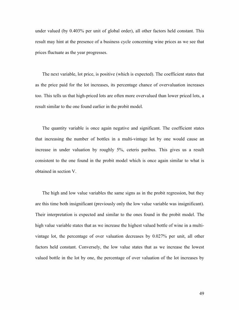
49

under valued (by 0.403% per unit of global order), all other factors held constant. This

result may hint at the presence of a business cycle concerning wine prices as we see that

prices fluctuate as the year progresses.

The next variable, lot price, is positive (which is expected). The coefficient states that

as the price paid for the lot increases, its percentage chance of overvaluation increases

too. This tells us that high-priced lots are often more overvalued than lower priced lots, a

result similar to the one found earlier in the probit model.

The quantity variable is once again negative and significant. The coefficient states

that increasing the number of bottles in a multi-vintage lot by one would cause an

increase in under valuation by roughly 5%, ceteris paribus. This gives us a result

consistent to the one found in the probit model which is once again similar to what is

obtained in section V.

The high and low value variables the same signs as in the probit regression, but they

are this time both insignificant (previously only the low value variable was insignificant).

Their interpretation is expected and similar to the ones found in the probit model. The

high value variable states that as we increase the highest valued bottle of wine in a multi-

vintage lot, the percentage of over valuation decreases by 0.027% per unit, all other

factors held constant. Conversely, the low value states that as we increase the lowest

valued bottle in the lot by one, the percentage of over valuation of the lot increases by

50

0.15%, ceteris paribus. Despite these results being statistically insignificant, their signs

and magnitudes are interpretable economically.

The three quality variables are statistically insignificant as they were in the probit

model. The coefficients state that increasing the maximum quality of a wine in a lot will

cause the percentage of over valuation to decrease. Conversely, decreasing the minimum

quality of the lot would increase the percentage of over valuation of that lot, ceteris

paribus. These results do not coincide with the probit model proposed earlier (since in the

probit a higher maximum favored over valuation and vice versa).

The lot composition dummies tell us that if the wines in the multi-vintage lot are all

from the same year, the percentage over valuation of that lot will increase by 11%, all

factors remaining equal. Conversely if a multi-vintage lot’s wines are all from the same

chateau or region, then their percentage of over valuation will fall. These coefficients are

not statistically significant.

From the above models we can see that many of our previously obtained results are

apparent in both the ordinary least squares model and the probit model. Whilst both

models have coefficients with different signs, the majority of the significant variables are

the same. We can see that factors such as the order of the lot (in the both the auction and

in the year) and the number of bottles in the lot will be significant in determining the over

or under valuation of a lot.

51

VII. Conclusion

The beginning of section V exhibited a study (summarized in table 4) which

examined the price per bottle with respect to lot size of three wines without taking into

account the particular characteristics of the wines. The conclusion of this study was that

as the lot size increased for these wines, so did the price per bottle, which coincides with

the study performed by Bentzen and Smith (2003). Section IV followed to perform two

regressions which took into account the particular characteristics of the wines to obtain

the semi elasticity of the price per bottle on the lot size. These regressions yielded a

negative semi elasticity concluding that increasing the number of bottles in a lot led to a

decrease of the price per bottle of that lot, the opposite of the initial study. Thus we can

see that not taking into account the particular characteristics of wines can lead to an

analysis with false conclusions about the price per bottle in increasing lot sizes.

Section VI concentrated on the characteristics of multi-vintage lots which cause them

to be over or under valued. Through probit and ordinary least squares regressions, we

were able to establish a positive and significant relationship between quantity and under

valuation. This stated a similar conclusion to the one found in section V: increasing lot

size would decrease the price paid per bottle, thus increasing the chance of the lot being

under valued. This yields a final conclusion which states that if an auctioneer wanted to

obtain the maximum price per bottle for each lot she sold, she would be best off selling

her wines individually, in single unit lots.

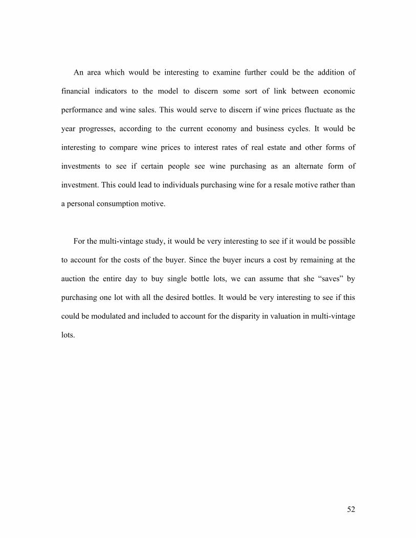
52

An area which would be interesting to examine further could be the addition of

financial indicators to the model to discern some sort of link between economic

performance and wine sales. This would serve to discern if wine prices fluctuate as the

year progresses, according to the current economy and business cycles. It would be

interesting to compare wine prices to interest rates of real estate and other forms of

investments to see if certain people see wine purchasing as an alternate form of

investment. This could lead to individuals purchasing wine for a resale motive rather than

a personal consumption motive.

For the multi-vintage study, it would be very interesting to see if it would be possible

to account for the costs of the buyer. Since the buyer incurs a cost by remaining at the

auction the entire day to buy single bottle lots, we can assume that she “saves” by

purchasing one lot with all the desired bottles. It would be very interesting to see if this

could be modulated and included to account for the disparity in valuation in multi-vintage

lots.

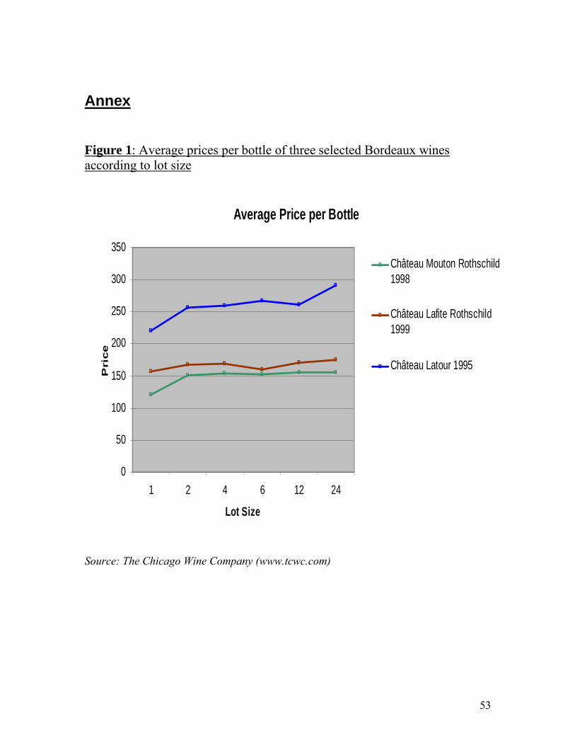
53

Annex

Figure 1: Average prices per bottle of three selected Bordeaux wines according to lot size

Average Price per Bottle

0

50

100

150

200

250

300

350

1 2 4 6 12 24

Lot Size

Pri

ce

Château Mouton Rothschild1998

Château Lafite Rothschild1999

Château Latour 1995

Source: The Chicago Wine Company (www.tcwc.com)

54

Figure 2: Wine producing region of Bordeaux in France

Source: Great wine capitals: Global Network (http://www.greatwinecapitals.com)

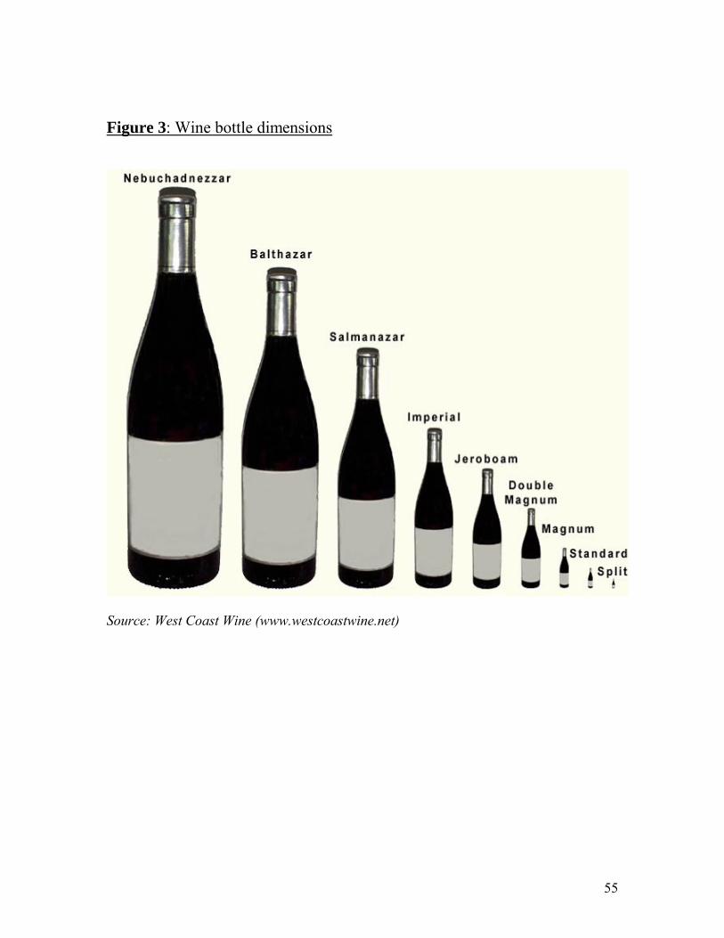
55

Figure 3: Wine bottle dimensions

Source: West Coast Wine (www.westcoastwine.net)

56

Figure 4: Greater Region Production in Bordeaux

Médoc15%

Graves8%

Rivers64%

Côtes13%

Médoc

Graves

Rivers

Côtes

Source: Terriors France (http://www.terroirs-france.com)

Figure 5: Sub-Region Production in Médoc Greater Region

Médoc34%

Haut Médoc30%

Margaux8%

St. Estèphe8%

Pauillac7%

Listrac4%

Moulis4%St. Julien

5%Médoc

Haut Médoc

Margaux

St. Estèphe

Pauillac

St. Julien

Moulis

Listrac


57

Figure 6: Sub-Region Production in Graves Greater Region

Graves36%

Pessac Léognan15%

Premières Côtes39%

Sauternes7%

Barsac3%

Graves

Pessac Léognan

Sauternes

Barsac

Premières Côtes


Figure 7: Sub-Region Production in Rivers Greater Region

Bordeaux Supérieur97%

Entre deux mers3%

Bordeaux Supérieur

Entre deux mers


58

Figure 8: Sub-Region Production in Côtes Greater Region

St. Emilion35%

Côtes de Castillon21%

Côtes de Francs3%

Pomerol5%

Fronsac6%

Côtes de Bourg30%

St. Emilion

Côtes de Castillon

Côtes de Francs

Pomerol

Fronsac

Côtes de Bourg


59

Table I: Greater and Sub-Region Wine Production Statistics

Area* % Production** %MEDOCMédoc 4900 32.89 40 33.70Haut Médoc 4250 28.52 36 30.33Margaux 1300 8.72 9.5 8.00St. Estèphe 1200 8.05 9 7.58Pauillac 1100 7.38 8.5 7.16St. Julien 900 6.04 6.5 5.48Moulis 550 3.69 4.2 3.54Listrac 700 4.70 5 4.21

GRAVESGraves 3000 29.18 22 35.89Pessac Léognan 1350 13.13 9 14.68Sauternes 1800 17.51 4.5 7.34Barsac 830 8.07 1.8 2.94Premières Côtes 3300 32.10 24 39.15

RIVERSBordeaux Supérieur 49000 95.33 475 96.94Entre deux mers 2400 4.67 15 3.06

COTESSt. Emilion 5500 37.70 36 34.65Côtes de Castillon 2900 19.88 22 21.17Côtes de Francs 490 3.36 3.6 3.46Pomerol 800 5.48 5.3 5.10Fronsac 1200 8.22 6 5.77Côtes de Bourg 3700 25.36 31 29.84

BORDEAUXMédoc 14900 16.34 118.7 15.34Graves 10280 11.28 61.3 7.92Rivers 51400 56.38 490 63.32Côtes 14590 16.00 103.9 13.43

* Denoted in hectares** Denoted in millions of bottles


60

Table II: Sub-Region production as a percentage of Entire Bordeaux Production

Sub-Region Area* % Production** %

Médoc 4900 5.37 40 5.17Haut Médoc 4250 4.66 36 4.65Margaux 1300 1.43 9.5 1.23St. Estèphe 1200 1.32 9 1.16Pauillac 1100 1.21 8.5 1.10St. Julien 900 0.99 6.5 0.84Moulis 550 0.60 4.2 0.54Listrac 700 0.77 5 0.65Graves 3000 3.29 22 2.84Pessac Léognan 1350 1.48 9 1.16Sauternes 1800 1.97 4.5 0.58Barsac 830 0.91 1.8 0.23Premières Côtes 3300 3.62 24 3.10Bordeaux Supérieur 49000 53.75 475 61.38Entre deux meres 2400 2.63 15 1.94St. Emilion 5500 6.03 36 4.65Côtes de Castillon 2900 3.18 22 2.84Côtes de Francs 490 0.54 3.6 0.47Pomerol 800 0.88 5.3 0.68Fronsac 1200 1.32 6 0.78Côtes de Bourg 3700 4.06 31 4.01

* Denoted in hectares** Denoted in millions of bottles


61

Table III: Summary of Sub-region dummies

Sub-region Lots*

Côtes de Bourg 43Côtes de Castillon 57Fronsac 39Graves 62 Greater Region Lots*Haut Médoc 51Margaux 582 Médoc 3087Médoc 18 Graves 716Pauillac 1569 Rivers 15Pessac Léognan 616 Côtes 3595Pomerol 1318Premières Côtes 38 Total 7413St. Emilion 2138St. Estèphe 326St. Julien 541Bordeaux Supérieur** 15

Total 7413

* Lots contain between 1 and 24 bottles of the same wine** Bordeaux Supérieur used as zero condition for dummy variables


62

Bibliography

Articles and Books:

Ashenfelter, Orley. “How auctions Work for Wine and Art.” Journal of Economic Perspectives, volume 3, no. 3 (1989): 23-36.

Bentzen, Jan, Valdemar Smith. “A Comparative Study of Wine Auction Prices: Mouton Rothschild Premier Cru Classé” Denmark: Department of Economics, Aarhus School of Business, 2003.

Greene, William H. Econometric Analysis. New Jersey: Pearson Education, Inc., 2003.

Jehle, Geoffrey A., Philip J. Reny. Advanced Microeconomic Theory, 2e. Addison-Wesley, 2000.

Lecocq, Sébastien, Thierry Magnac, Marie-Claude Pichery, and Michael Vissier. “The impact of information on wine auction prices: results of an experiment.” Paris: INRA, INRA-LEA, LATEC, and CREST, 2003.

Varian, Hal R. Intermediate Microeconomics: A Modern Approach, 5e. New York: W. W. Norton & Company, Inc., 1999

Vickrey, William. “Counterspeculation, Auctions, and Competitive SealedTenders.” Journal of Finance, volume 16, no. 1 (1961): 8-37.

Wooldridge, Jeffrey M. Introductory Econometrics: A Modern Approach, 2e. Mason: South-Western, 2003.

63

Internet sources:

Cantor, Abbey. “A toast to Bloomington with Oliver Winery.” Bloomington @ Work. Ed. Katie Halpern. <http://www.journalism.indiana.edu/gallery/j201fall03/Bloomington@Work/KatieFinal>

e Robert Parker. <http://www.erobertparker.com>

Euromonitor International: <http://www.euromonitor.com>

Great Wine Capitals, Global Network. <http://www.greatwinecapitals.com/>

LaMar, Jim. “Wine and Health… Benefits are without cautions.” Professional Friends of Wine. <http://www.winepros.org>

Napa Valley Wineries. <http://www.napavintners.com>

Phillip Shull. “South Korea, a Booming Market for U.S. Wine Exports.” USDA Foreign Agricultural Service. 2004 <http://www.fas.usda.gov>

Research and Markets. “Wine in China: A Market Analysis.” 2005 <http://www.researchandmarkets.com>

Rice Unix Facility. “FAQs: Statistical Interaction in Multiple Regression.” 1999. <http://www.ruf.rice.edu/~branton/interaction/faqshome.htm>

Rogov, Daniel. “A History of Wine.” Jewish Virtual Library. 2006. <http://www.jewishvirtuallibrary.org>

Terroir-France. <http://www.terroir-france.com>

The Chicago Wine Company. <http://www.tcwc.com>

Townsend Real Estate. “Buyers Premium.” 2005. <http://www.townsend-real-estate.com/Buyers_Premium.htm>

a study of auctioneer’s decisions

Documents