Real3D

A Structural Analysis and Design Program

Accuracy, Reliability, Ease of Use

Computations & Graphics, Inc. 5290 Windflower Lane

Highlands Ranch, CO 80130, USA

Email: info@cg-inc.com Web: www.cg-inc.com

i

End User License Agreement for CGI Software The Software is protected by United States copyright laws and various international treaties. By installing or using the Software, you agree to be bound by the terms of this Agreement. If you do not agree with the terms of this Agreement, do not install or use the Software. This Agreement is governed by the laws of the United States and the State of Colorado. 1. DEFINITIONS “Software” means all of the contents of the files, disk(s), CD-ROM(s) or other media with which this Agreement is provided. “Documentation” means all of the contents of the files, printed materials with which this Agreement is provided. “End User” means you. “CGI” means Computations & Graphics, Inc. 2. GRANT OF LICENSE a). The following applies if you have purchased a perpetual Software license: CGI grants you (the End User) a non-exclusive, non-transferable license to use the Software on a single computer. You may not rent, lease, or resell the Software. You may not disassemble, decompile, reverse engineer or modify the Software in any way. This License starts from the date you receive the Software and will last as long as the End User complies with the terms of this Agreement. b). The following applies if you have purchased a subscription Software license: CGI grants you (the End User) a non-exclusive, non-transferable license to use the Software simultaneously via internet on a certain number of computers for a certain subscription period. You may not rent, lease, or resell the Software. You may not disassemble, decompile, reverse engineer or modify the Software in any way. This License starts from the date you purchased the subscription license and will last for the subscription period. 3. SUPPORT CGI offers limited 30 days free email technical support related to the installation and uses of the most recent version of Software, starting from the start date of this Agreement. CGI has no obligation to provide support in any form if your version of the Software is not the most recent version. CGI, in its sole discretion, will determine what constitutes a support incident. CGI reserves the right to refuse support service to anyone. 4. COPYRIGHT The Software and Documentation are the intellectual property of and are owned by CGI. You may make at most one copy of the Software and/or the Documentation for backup purposes. 5. COMMERCIAL USES The evaluation, educational and beta versions of the Software may not be used for commercial purposes. 6. LIMITATION OF LIABILITY IN NO EVENT WILL CGI OR ITS SUPPLIERS BE LIABLE TO YOU FOR ANY DAMAGES, CLAIMS OR COSTS WHATSOEVER OR ANY CONSEQUENTIAL, INDIRECT, INCIDENTAL DAMAGES, OR ANY LOST PROFITS OR LOST SAVINGS, EVEN IF CGI HAS BEEN ADVISED OF THE POSSIBILITY OF SUCH LOSS, DAMAGES, CLAIMS OR COSTS. 7. DISCLAIMER CGI HAS TAKEN EVERY EFFORT TO MAKE THE SOFTWARE RELIABLE AND ACCURATE. HOWEVER, IT IS THE END USER’S RESPONSIBILITY TO INDEPENDENTLY VERIFY THE ACCURACY AND RELIABLITY OF THE SOFTWARE. NO EXPRESS OR IMPLIED WARRANTY IS PROVIDED BY CGI OR ITS DEVELOPERS ON THE ACCURACY OR RELIABILITY OF THE SOFTWARE.

ii

Copyright

THE SOFTWARE REAL3D (FORMERLY REAL3D-ANALYSIS) AND ALL ITS DOCUMENTATION ARE THE INTELLECTUAL PROPERTY OF AND ARE OWNED BY COMPUTATIONS & GRAPHICS INC. (CGI). ILLEGAL USE OF THE SOFTWARE OR REPRODUCTION OF ITS DOCUMENTATION IS STRICTLY PROHIBITED.

Disclaimer

CGI HAS TAKEN EVERY EFFORT TO MAKE THE SOFTWARE RELIABLE AND ACCURATE. HOWEVER, IT IS THE END USER’S RESPONSIBILITY TO INDEPENDENTLY VERIFY THE ACCURACY AND RELIABLITY OF THE SOFTWARE. NO EXPRESS OR IMPLIED WARRANTY IS PROVIDED BY CGI OR ITS DEVELOPERS ON THE ACCURACY OR RELIABILITY OF THE SOFTWARE.

Notice SINCE REAL3D COMES IN DIFFERENT VERSIONS, SOME FEATURES DESCRIBED IN THIS DOCUMENTATION MAY NOT APPLY TO THE SPECIFIC VERSION OF THE PROGRAM YOU ARE RUNNING. OpenGL® is a registered trademark of Hewlett Packard Enterprise. Windows® is a registered trademark of Microsoft Corporation. Real3D is a trademark of Computations & Graphics, Inc. Copyright 2002-2020 by Computations & Graphics, Inc. All rights reserved. Last Revised Nov. 2019

iii

Terms and Conventions The convention for commands in this documentation is Main Menu | Sub-Menu. For example, Edit | Undo means the Undo command from the Edit main menu. Model View: A window in the program that contains the graphical display of the model. Report View: A window in the program that contains the text or graphical report. Structural Command: A command in the program that affects the results for a model. Member: A beam or frame element. It also refers to a truss when the element has full moment releases at two ends. The term “beam element”, “frame element” and “member” are used interchangeably in this program. Shell: a four node shell finite element. It includes membrane action and plate bending action. It is sometimes called shell4. Brick : a eight node solid finite element. Element: A member or finite element (shell or brick). Object: A node or finite element (shell or brick) or its dependent. Dependent: A structural entity whose existence depends upon the existence of another structural entity. For example, a support is a dependent of a node; a moment release is a dependent of a member (beam element). All loads are dependents of nodes or members or finite elements. Parent: A structural entity which may have dependents. Nodes and elements may be parents. For example, a node may be a parent of a support or a member. A member may be a parent of a moment release. Distance List: A comma separated list that specifies multiple distances. For example, a distance list of “12,2@14,3@10” will generate distances of 12, 14, 14, 10, 10, and 10 in length units. Orphaned Node: A node that is not connected to any elements. DOFs: Degrees of freedom. 64-bit floating point (double precision): The solver that uses 64-bit (8 bytes) floating-point arithmetics. The 64-bit floating point (double precision) is the standard solver in almost all structural analysis programs. 128-bit floating point (quad precision): The solver that uses 128-bit (16 bytes) floating-point arithmetics. The 128-bit floating point (quad precision) is extremely accurate and is uniquely available in Real3D.

iv

Table of Contents

END USER LICENSE AGREEMENT FOR CGI SOFTWARE .................................................................................................................. I COPYRIGHT ................................................................................................................................................................................... II DISCLAIMER .................................................................................................................................................................................. II NOTICE .......................................................................................................................................................................................... II TERMS AND CONVENTIONS .......................................................................................................................................................... III INTRODUCTION .............................................................................................................................................................................. 1

Graphical User Interface (GUI) .............................................................................................................................................. 2 Command Window ................................................................................................................................................................... 2 Enter Nodal Coordinates ......................................................................................................................................................... 3 Mouse Use ............................................................................................................................................................................... 4 Spreadsheet Navigation ........................................................................................................................................................... 4 System Requirements ............................................................................................................................................................... 5

MENUS ........................................................................................................................................................................................... 6

MENU OVERVIEW .......................................................................................................................................................................... 7 CHAPTER 1: FILE ....................................................................................................................................................................... 17

New ........................................................................................................................................................................................ 17 Open....................................................................................................................................................................................... 17 Close ...................................................................................................................................................................................... 18 Save ........................................................................................................................................................................................ 18 Save As ................................................................................................................................................................................... 18 Save All .................................................................................................................................................................................. 18 Append File ............................................................................................................................................................................ 18 Import from DXF ................................................................................................................................................................... 19 Import from SAP2000 .s2k ..................................................................................................................................................... 20 Export to DXF ........................................................................................................................................................................ 20 Batch Run | Batch Static Analysis .......................................................................................................................................... 21 Batch Run | Batch Frequency Analysis .................................................................................................................................. 21 Batch Run | Batch Concrete Design ...................................................................................................................................... 21 Batch Run | Batch Steel Design ............................................................................................................................................. 21 Batch Run | Batch Text Report ............................................................................................................................................... 21 Advanced | Generate SolverBlaze Source Code .................................................................................................................... 21 Print Setup (Model View) ...................................................................................................................................................... 22 Print Setup (Report View) ...................................................................................................................................................... 22 Print Preview (Report View) .................................................................................................................................................. 23 Print (Report View) ................................................................................................................................................................ 23 Print Current View ................................................................................................................................................................ 23 Capture Images | Capture Current Image ............................................................................................................................. 23 Capture Images | Delete All Images ...................................................................................................................................... 23 Capture Images | Print Captured Images .............................................................................................................................. 23 General Information .............................................................................................................................................................. 23 Text Report............................................................................................................................................................................. 24 Envelope Report ..................................................................................................................................................................... 24 Statistics ................................................................................................................................................................................. 27 View Log File ......................................................................................................................................................................... 27 Open Containing Folder ........................................................................................................................................................ 27

CHAPTER 2: EDIT ...................................................................................................................................................................... 28 Undo ...................................................................................................................................................................................... 28 Redo ....................................................................................................................................................................................... 28 Lock Model ............................................................................................................................................................................ 28 Duplicate ............................................................................................................................................................................... 28 Array ...................................................................................................................................................................................... 29 Mirror .................................................................................................................................................................................... 29 Move ...................................................................................................................................................................................... 30 Rotate ..................................................................................................................................................................................... 30 Scale ....................................................................................................................................................................................... 30 Delete ..................................................................................................................................................................................... 31

v

Extrude | Extrude Nodes to Members .................................................................................................................................... 31 Extrude | Extrude Members to Shell4s ................................................................................................................................... 32 Extrude | Extrude Shell4s to Bricks ....................................................................................................................................... 33 Revolve | Revolve Members to Shell4s ................................................................................................................................... 33 Revolve | Revolve Shell4s to Bricks ....................................................................................................................................... 34 Split Members ........................................................................................................................................................................ 35 Sub-Mesh Shell4s ................................................................................................................................................................... 36 Insert Nodes at Intersections of Selected Members ............................................................................................................... 37 Explode Selected Members at Nodes ..................................................................................................................................... 37 Re-Number | Auto Number All Nodes .................................................................................................................................... 37 Re-Number | Re-Number Selected Nodes .............................................................................................................................. 38 Re-Number | Re-Number Selected Members ......................................................................................................................... 38 Re-Number | Re-Number Selected Shell4s ............................................................................................................................. 38 Re-Number | Re-Number Selected Bricks .............................................................................................................................. 38 Switch Coordinates ................................................................................................................................................................ 38 Reverse Node Order for Selected Elements ........................................................................................................................... 39 Merge All Nodes & Elements ................................................................................................................................................. 39 Remove All Orphaned Nodes ................................................................................................................................................. 39 Element Local Angle .............................................................................................................................................................. 39 Match Local x-Axes for Shells ............................................................................................................................................... 40 3-Point Member Orientation.................................................................................................................................................. 40 Tension/Compression Only .................................................................................................................................................... 41 Convert Selected Members to Rigid Links ............................................................................................................................. 41 Self Weight Exclusion ............................................................................................................................................................ 41 Element Activation ................................................................................................................................................................. 41 Clear | Clear Undo & Redo ................................................................................................................................................... 42 Clear | Clear Results.............................................................................................................................................................. 42 Clear | Clear Everything ........................................................................................................................................................ 42

CHAPTER 3: VIEW ..................................................................................................................................................................... 43 Redraw ................................................................................................................................................................................... 43 Restore Model ........................................................................................................................................................................ 43 Preset Views........................................................................................................................................................................... 43 Named Views ......................................................................................................................................................................... 43 Named Selections ................................................................................................................................................................... 44 Zoom | Zoom Extent ............................................................................................................................................................... 44 Zoom | Zoom Window ............................................................................................................................................................ 44 Zoom | Zoom Object .............................................................................................................................................................. 44 Zoom | Zoom Previous ........................................................................................................................................................... 44 Zoom | Zoom In ...................................................................................................................................................................... 45 Zoom | Zoom Out ................................................................................................................................................................... 45 Pan | Pan Screen ................................................................................................................................................................... 45 Pan | Left................................................................................................................................................................................ 45 Pan | Right ............................................................................................................................................................................. 45 Pan | Up ................................................................................................................................................................................. 45 Pan | Down ............................................................................................................................................................................ 45 Rotate | +X ............................................................................................................................................................................. 46 Rotate | -X .............................................................................................................................................................................. 46 Rotate | +Y ............................................................................................................................................................................. 46 Rotate | -Y .............................................................................................................................................................................. 46 Rotate | +Z ............................................................................................................................................................................. 46 Rotate | -Z .............................................................................................................................................................................. 46 Real Time Motion | Real-Time Pan ....................................................................................................................................... 46 Real Time Motion | Real-Time Zoom ..................................................................................................................................... 47 Real Time Motion | Real-Time Rotate.................................................................................................................................... 47 Window/Point Select .............................................................................................................................................................. 47 Line Select .............................................................................................................................................................................. 47 Select by IDs | Nodes ............................................................................................................................................................. 47 Select by IDs | Members ........................................................................................................................................................ 48 Select by IDs | Shell4s ............................................................................................................................................................ 48 Select by IDs | Bricks ............................................................................................................................................................. 48

vi

Select by IDs | Select All ........................................................................................................................................................ 48 Select by IDs | Unselect All .................................................................................................................................................... 48 Select by Properties | Materials ............................................................................................................................................. 48 Select by Properties | Member Sections ................................................................................................................................. 49 Select by Properties | Orientations ........................................................................................................................................ 49 Select by Properties | Tension Only Members ....................................................................................................................... 50 Select by Properties | Compression Only Members ............................................................................................................... 50 Select by Properties | Shell Thicknesses ................................................................................................................................ 50 Select by Properties | Orphaned Nodes ................................................................................................................................. 50 Select by Properties | Coordinates ........................................................................................................................................ 51 Select by Properties | Selection Names .................................................................................................................................. 51 Select by Properties | Concrete Beam Criteria ...................................................................................................................... 52 Select by Properties | Concrete Column Criteria .................................................................................................................. 52 Select by Properties | Concrete Plate Criteria ...................................................................................................................... 52 Select by Properties | Steel Design Criteria .......................................................................................................................... 52 Select by Properties | Unity Check Ratios ............................................................................................................................. 52 Select by Properties | Select All ............................................................................................................................................. 52 Select by Properties | Unselect All ......................................................................................................................................... 52 Flip Selection ......................................................................................................................................................................... 53 Freeze Selected ...................................................................................................................................................................... 53 Freeze All Except Selected ..................................................................................................................................................... 53 Freeze All Except Level ......................................................................................................................................................... 53 Freeze All Except Plane ......................................................................................................................................................... 53 Thaw ...................................................................................................................................................................................... 54 Load Diagram ........................................................................................................................................................................ 54 Annotate ................................................................................................................................................................................. 55 Query ..................................................................................................................................................................................... 55 Distance ................................................................................................................................................................................. 55 Render | Render Options ........................................................................................................................................................ 56 Render | Quick Render ........................................................................................................................................................... 57 Result Diagrams | Shear and Moment Diagram .................................................................................................................... 57 Result Diagrams | Deflection Diagram ................................................................................................................................. 57 Result Diagrams | Contour Diagram ..................................................................................................................................... 58 Result Diagrams | Mode Shape .............................................................................................................................................. 59 Result Diagrams | Unity Check .............................................................................................................................................. 60 Result Diagrams | Response Animation ................................................................................................................................. 60 Options | Drawing Grid ......................................................................................................................................................... 60 Options | Global Axes ............................................................................................................................................................ 60 Options | Contour Legend ...................................................................................................................................................... 61 Options | Comment ................................................................................................................................................................ 61

CHAPTER 4: GEOMETRY ............................................................................................................................................................ 62 Materials ................................................................................................................................................................................ 62 Sections .................................................................................................................................................................................. 63 Thicknesses ............................................................................................................................................................................ 65 Levels ..................................................................................................................................................................................... 66 Drawing Grid......................................................................................................................................................................... 67 Object Snap ............................................................................................................................................................................ 68 Draw Node ............................................................................................................................................................................. 68 Draw Member ........................................................................................................................................................................ 68 Draw Shell4 ........................................................................................................................................................................... 69 Draw Brick............................................................................................................................................................................. 69 Quick Draw | Member ........................................................................................................................................................... 70 Quick Draw | Shell4 ............................................................................................................................................................... 70 Quick Draw | Brick ................................................................................................................................................................ 70 Generate ................................................................................................................................................................................ 70 Generate | Rectangular Frames ............................................................................................................................................. 71 Generate | Cylindrical Frames .............................................................................................................................................. 73 Generate | Rectangular Shell4s ............................................................................................................................................. 74 Generate | Circular Shell4s ................................................................................................................................................... 75 Generate | Arc Members ........................................................................................................................................................ 75

vii

Generate | Non-Prismatic Members ...................................................................................................................................... 76 Generate | Nodes from Grid .................................................................................................................................................. 77 Generate | Members by Nodes ............................................................................................................................................... 77 Generate | Shells by Nodes .................................................................................................................................................... 79 Generate | Bricks by Nodes.................................................................................................................................................... 79 Element Local Angle .............................................................................................................................................................. 79 3-Point Member Orientation.................................................................................................................................................. 79 Moment Releases ................................................................................................................................................................... 80 Rigid Offset ............................................................................................................................................................................ 80 Tension/Compression Only .................................................................................................................................................... 81 Convert Members to Rigid Links ........................................................................................................................................... 81 Element Activation ................................................................................................................................................................. 81 Supports ................................................................................................................................................................................. 81 Springs ................................................................................................................................................................................... 82 Coupled Springs ..................................................................................................................................................................... 83 Diaphragms ........................................................................................................................................................................... 84 Multi-DOF Constraints | Inclined Rollers ............................................................................................................................. 84 Multi-DOF Constraints | Equal Displacement Constraints ................................................................................................... 85 Multi-DOF Constraints | Generic Constraints ...................................................................................................................... 86 Story Drift Nodes ................................................................................................................................................................... 86

CHAPTER 5: LOADS ................................................................................................................................................................... 87 Load Cases............................................................................................................................................................................. 87 Load Combinations ................................................................................................................................................................ 87 Nodal Loads ........................................................................................................................................................................... 89 Point Loads ............................................................................................................................................................................ 90 Line Loads ............................................................................................................................................................................. 91 Area Loads ............................................................................................................................................................................. 91 Surface Loads ........................................................................................................................................................................ 92 Thermal Loads ....................................................................................................................................................................... 93 Self Weights ........................................................................................................................................................................... 93 Self Weight Exclusion ............................................................................................................................................................ 94 Generate Loads | Fluid Loads ............................................................................................................................................... 94 Generate Loads | Pattern Loads ............................................................................................................................................ 94 Generate Loads | Moving Loads ............................................................................................................................................ 95 Case-Copy Loads ................................................................................................................................................................... 96 Convert Area Loads to Line Loads ........................................................................................................................................ 96 Convert Local Loads to Global Loads ................................................................................................................................... 97 Additional Masses .................................................................................................................................................................. 97 Response Spectra Library ...................................................................................................................................................... 97

CHAPTER 5A: ASSIGN ............................................................................................................................................................... 99 Supports ................................................................................................................................................................................. 99 Springs ................................................................................................................................................................................... 99 Member Properties ................................................................................................................................................................ 99 Shell Properties ................................................................................................................................................................... 101 Nodal Loads ......................................................................................................................................................................... 101 Point Loads .......................................................................................................................................................................... 101 Line Loads ........................................................................................................................................................................... 102 Surface Loads ...................................................................................................................................................................... 102 Additional Masses ................................................................................................................................................................ 103 Deletion ............................................................................................................................................................................... 103

CHAPTER 6: INPUT DATA ........................................................................................................................................................ 105 Properties | Materials .......................................................................................................................................................... 105 Properties | Sections ............................................................................................................................................................ 105 Properties | Thicknesses ...................................................................................................................................................... 105 Nodes ................................................................................................................................................................................... 105 Members .............................................................................................................................................................................. 106 Shell4s .................................................................................................................................................................................. 106 Bricks ................................................................................................................................................................................... 107 Supports ............................................................................................................................................................................... 108 Springs | Nodal Springs ....................................................................................................................................................... 109

viii

Springs | Coupled Springs ................................................................................................................................................... 109 Springs | Line Springs .......................................................................................................................................................... 110 Springs | Surface Springs ..................................................................................................................................................... 110 Moment Releases ................................................................................................................................................................. 111 Diaphragms ......................................................................................................................................................................... 111 Multi-DOF Constraints ........................................................................................................................................................ 112 Load Cases........................................................................................................................................................................... 113 Load Combinations .............................................................................................................................................................. 113 Nodal Loads ......................................................................................................................................................................... 113 Point Loads .......................................................................................................................................................................... 113 Line Loads ........................................................................................................................................................................... 114 Area Loads ........................................................................................................................................................................... 115 Surface Loads ...................................................................................................................................................................... 116 Thermal Loads | Member Thermal Loads ............................................................................................................................ 117 Thermal Loads | Shell Thermal Loads ................................................................................................................................. 117 Thermal Loads | Brick Thermal Loads ................................................................................................................................ 118 Self Weights ......................................................................................................................................................................... 119 Calculated Masses ............................................................................................................................................................... 119 Additional Masses ................................................................................................................................................................ 119 Response Spectra Library .................................................................................................................................................... 121 Drift Nodes........................................................................................................................................................................... 121 Comments ............................................................................................................................................................................ 122

CHAPTER 7: ANALYSIS ............................................................................................................................................................ 123 Analysis Options .................................................................................................................................................................. 123 Static Analysis ...................................................................................................................................................................... 126 Frequency Analysis .............................................................................................................................................................. 126 Response Spectrum Analysis ................................................................................................................................................ 127

CHAPTER 8: ANALYSIS RESULT .............................................................................................................................................. 129 Nodal Displacements ........................................................................................................................................................... 129 Story Drifts........................................................................................................................................................................... 129 Support Reactions ................................................................................................................................................................ 130 Spring Reactions | Nodal ..................................................................................................................................................... 130 Spring Reactions | Coupled ................................................................................................................................................. 130 Spring Reactions | Line ........................................................................................................................................................ 130 Spring Reactions | Surface ................................................................................................................................................... 131 Multi-DOF Constraint Forces & Moments ......................................................................................................................... 131 Member End Forces & Moments ......................................................................................................................................... 132 Member Segmental Results .................................................................................................................................................. 132 Shell4 Forces & Moments .................................................................................................................................................... 132 Shell4 Principal Forces & Moments .................................................................................................................................... 133 Shell4 Stresses [Top] ........................................................................................................................................................... 133 Shell4 Stresses [Bottom] ...................................................................................................................................................... 133 Shell4 Principal Stresses ..................................................................................................................................................... 134 Shell4 Nodal Resultants ....................................................................................................................................................... 134 Brick Stresses ....................................................................................................................................................................... 135 Brick8 Principal Stresses ..................................................................................................................................................... 135 Envelope | Nodal Displacements ......................................................................................................................................... 136 Envelope | Support Reactions .............................................................................................................................................. 137 Envelope | Member Segmental Results ................................................................................................................................ 138 Eigenvalues .......................................................................................................................................................................... 138 Eigenvectors ........................................................................................................................................................................ 139 Mode Participation Factors ................................................................................................................................................. 139 Modal Displacements | Modal Displacements SX, SY and SZ ............................................................................................. 140 Inertia Forces | Inertia Forces SX, SY and SZ ..................................................................................................................... 140 Modal Combinations | Nodal Displacements ...................................................................................................................... 140 Modal Combinations | Support Reactions ........................................................................................................................... 141 Modal Combinations | Nodal, Coupled, Line, Surface Spring Reactions ............................................................................ 141 Modal Combinations | Multi-DOF Constraint Forces & Moments ..................................................................................... 141 Modal Combinations | Member End Forces & Moments .................................................................................................... 142 Modal Combinations | Member Segmental Results ............................................................................................................. 142

ix

Modal Combinations | Shell4 Forces & Moments ............................................................................................................... 143 Modal Combinations | Brick Stresses .................................................................................................................................. 143 Modal Combinations | Base Shears ..................................................................................................................................... 143

CHAPTER 9: CONCRETE DESIGN .............................................................................................................................................. 145 RC Materials ........................................................................................................................................................................ 145 Design Criteria | Model Design Criteria ............................................................................................................................. 145 Design Criteria | Beam Design Criteria .............................................................................................................................. 147 Design Criteria | Column Design Criteria .......................................................................................................................... 148 Design Criteria | Plate Design Criteria ............................................................................................................................... 149 Design Criteria | Exclude Elements ..................................................................................................................................... 150 Design Criteria | Cracking Factors ..................................................................................................................................... 150 Assign | Beam Design Properties ........................................................................................................................................ 151 Assign | Column Design Properties ..................................................................................................................................... 151 Assign | Plate Design Properties ......................................................................................................................................... 152 Design Input | RC Member Input ......................................................................................................................................... 152 Design Input | RC Plate Input .............................................................................................................................................. 153 Perform Design .................................................................................................................................................................... 153 Design Output | RC Analysis Envelope................................................................................................................................ 153 Design Output | RC Beam Results ....................................................................................................................................... 154 Design Output | RC Column Results .................................................................................................................................... 155 Design Output | Flexural/Axial Interaction | Sections ......................................................................................................... 155 Design Output | Flexural/Axial Interaction | P-Mx (+) ....................................................................................................... 156 Design Output | Flexural/Axial Interaction | P-Mx (-) ........................................................................................................ 157 Design Output | Flexural/Axial Interaction | P-My (+) ....................................................................................................... 157 Design Output | Flexural/Axial Interaction | P-My (-) ........................................................................................................ 157 Design Output | Flexural/Axial Interaction | P-Mx-My ....................................................................................................... 157 Design Output | Flexural/Axial Interaction | Print Diagrams ............................................................................................. 157 Design Output | Member Shear Design ............................................................................................................................... 159 Design Output | Wood-Armer Moments............................................................................................................................... 159 Design Output | RC Plate Results ........................................................................................................................................ 159 Diagrams| RC Member Envelope Diagram ......................................................................................................................... 160 Diagrams | RC Plate Envelope Contour .............................................................................................................................. 160 RC Report ............................................................................................................................................................................ 161 RC Tools | Rebar Database ................................................................................................................................................. 163 RC Tools | K Calculator ...................................................................................................................................................... 163 RC Tools | Quick R-Beam Flexural Design ......................................................................................................................... 164 RC Tools | Quick T-Beam Flexural Design ......................................................................................................................... 164

CHAPTER 10: STEEL DESIGN ................................................................................................................................................... 165 Steel Materials ..................................................................................................................................................................... 165 Design Criteria | Model Design Criteria ............................................................................................................................. 165 Design Criteria | Member Design Criteria .......................................................................................................................... 166 Design Criteria | Section Pool ............................................................................................................................................. 167 Design Criteria | Exclude Elements ..................................................................................................................................... 168 Assign Member Design Properties ...................................................................................................................................... 168 Design Input | Steel Member Input ...................................................................................................................................... 169 Perform Design .................................................................................................................................................................... 169 Design Result ....................................................................................................................................................................... 169 Steel Tools | Section Check .................................................................................................................................................. 170 Steel Tools | Section Design ................................................................................................................................................. 179

CHAPTER 11: SETTINGS .......................................................................................................................................................... 180 Units & Precisions ............................................................................................................................................................... 180 Data Options ........................................................................................................................................................................ 181 New Origin........................................................................................................................................................................... 182 Vertical Axis......................................................................................................................................................................... 182 Graphic Scales ..................................................................................................................................................................... 183 Colors .................................................................................................................................................................................. 183 Preferences .......................................................................................................................................................................... 184 Enable/Disable Hardware Acceleration .............................................................................................................................. 185 Tools | Unit Conversion ....................................................................................................................................................... 185 Tools | Calculator ................................................................................................................................................................ 186

x

Tools | Text Editor ............................................................................................................................................................... 186 Tools | Copy Command History ........................................................................................................................................... 186 Tools | Clear Command History .......................................................................................................................................... 186 Toolbars | Main Toolbar ...................................................................................................................................................... 186 Toolbars | View Toolbar ...................................................................................................................................................... 186 Toolbars | Edit/Run Toolbar ................................................................................................................................................ 186 Toolbars | Input Toolbar ...................................................................................................................................................... 186 Toolbars | Output Toolbar ................................................................................................................................................... 186 Toolbars | Command Bar .................................................................................................................................................... 187 Toolbars | Status Bar ........................................................................................................................................................... 187

CHAPTER 12: WINDOW ........................................................................................................................................................... 188 New Window ........................................................................................................................................................................ 188 Close .................................................................................................................................................................................... 188 Close All .............................................................................................................................................................................. 188 Tile Horizontal ..................................................................................................................................................................... 188 Tile Vertical ......................................................................................................................................................................... 188 Tile Cascade ........................................................................................................................................................................ 188

TECHNICAL ISSUES ........................................................................................................................................................... 189

CHAPTER 13: COORDINATE SYSTEMS ..................................................................................................................................... 190 Global Coordinate System ................................................................................................................................................... 190 Local Coordinate Systems - General ................................................................................................................................... 190 Member Local Coordinate System ....................................................................................................................................... 191 Four-Node Shell Local Coordinate System ......................................................................................................................... 192 Eight-Node Brick Local Coordinate System ........................................................................................................................ 194

CHAPTER 14: NODES ............................................................................................................................................................... 195 Nodal Coordinates ............................................................................................................................................................... 195 Degrees of Freedom (DOFs) ............................................................................................................................................... 195 Node Numbers ..................................................................................................................................................................... 195 Loads ................................................................................................................................................................................... 196 Supports ............................................................................................................................................................................... 196 Multi-DOF Constraints ........................................................................................................................................................ 197 Nodal Springs ...................................................................................................................................................................... 197 Coupled Springs ................................................................................................................................................................... 198

CHAPTER 15: MEMBERS .......................................................................................................................................................... 199 Member Sections .................................................................................................................................................................. 199 Local Coordinate System ..................................................................................................................................................... 199 Member Numbers ................................................................................................................................................................. 199 Beams Vs. Trusses ............................................................................................................................................................... 200 Elastic Stiffness Matrix ........................................................................................................................................................ 200 Geometric Stiffness Matrix .................................................................................................................................................. 200 Moment Releases ................................................................................................................................................................. 201 Tension/Compression Only .................................................................................................................................................. 201 Rigid Links ........................................................................................................................................................................... 202 Rigid Diaphragms ................................................................................................................................................................ 202 Loads ................................................................................................................................................................................... 202 Line Springs ......................................................................................................................................................................... 206 Internal Forces and Moments .............................................................................................................................................. 207

CHAPTER 16: SHELLS .............................................................................................................................................................. 209 Shell Thicknesses ................................................................................................................................................................. 210 Local Coordinate System ..................................................................................................................................................... 210 Shell Numbers ...................................................................................................................................................................... 210 Element In-Plane Stiffness Matrix ....................................................................................................................................... 210 Element Out-of-Plane Stiffness Matrix ................................................................................................................................ 211 Combining Element In-Plane and Out-of-Plane Stiffness Matrices .................................................................................... 211 Loads ................................................................................................................................................................................... 211 Surface Springs .................................................................................................................................................................... 211 Internal Forces or Moments ................................................................................................................................................ 212 Membrane Nodal Resultants ................................................................................................................................................ 213

xi

CHAPTER 17: SOLIDS .............................................................................................................................................................. 215 Local Coordinate System ..................................................................................................................................................... 215 Solid Numbers ...................................................................................................................................................................... 215 Element Stiffness Matrix ...................................................................................................................................................... 215 Loads ................................................................................................................................................................................... 216 Internal Stresses ................................................................................................................................................................... 216

CHAPTER 18: STATIC ANALYSIS ............................................................................................................................................. 217 Load Cases and Load Combinations ................................................................................................................................... 217 Linear, Non-linear Static Analyses ...................................................................................................................................... 217 P-Delta (P-Δ) vs. P-delta (P-δ) ............................................................................................................................................ 218 Solution Algorithm ............................................................................................................................................................... 219 Solution Accuracy and Stability ........................................................................................................................................... 220

CHAPTER 19: FREQUENCY ANALYSIS ..................................................................................................................................... 223 Solution Algorithm ............................................................................................................................................................... 223 Mass and Stiffness ................................................................................................................................................................ 223 Solution Convergence .......................................................................................................................................................... 224

CHAPTER 19A: RESPONSE SPECTRUM ANALYSIS.................................................................................................................... 225 Solution Algorithm ............................................................................................................................................................... 225 Modal Combination ............................................................................................................................................................. 225 Directional Combination ..................................................................................................................................................... 226

CHAPTER 20: CONCRETE DESIGN – ACI 318-02/05/08/11/14 ................................................................................................. 227 Concrete Column Design ..................................................................................................................................................... 227 Concrete Beam Design ........................................................................................................................................................ 237 Concrete Slab/Wall Design .................................................................................................................................................. 241

CHAPTER 21: STEEL DESIGN – AISC 14TH EDITION LRFD ...................................................................................................... 243

Section Orientation .............................................................................................................................................................. 243 Member Internal Forces and Moments ................................................................................................................................ 244

REFERENCES ............................................................................................................................................................................. 246 APPENDIX .................................................................................................................................................................................. 248

Unit Conversions ................................................................................................................................................................. 248 Designations, diameters and areas of standard bars ........................................................................................................... 248

*************************************************** ******

1

Introduction Built from the ground up, Real3D (formerly Real3D-Analysis) is a powerful structural design / finite element analysis software tool designed for structural engineers of all skill levels. Real3D is reliable, easy to use, and affordable. The software is designed for accuracy and simplicity, allowing engineers to get the job done without being overwhelming by useless features. It is available in version optimized for either 32 bit or 64 bit Windows operating systems (Windows 7, 8 and 10). The program includes the following frame and finite elements:

- 2D and 3D beam and truss element (also called member). The element can be linear, tension only or compression only.

- 3D four-node shell element, with thick (MITC4) plate and thin (Kirchhoff) plate bending and plane membrane stress (compatible and incompatible) formulations.

- 3D eight-node solid element (brick) with compatible and incompatible formulations. - Linear and nonlinear nodal, line, and surface spring elements. - Coupled springs. - Rigid diaphragm, rigid link, multi-DOF constraints.

The program includes the following analysis and design options:

- Static linear analysis. - Geometric nonlinear (P-Delta) analysis. - Frequency (eigenvalue) analysis. - Response spectrum analysis. - Standard 64-bit floating point (double precision) and extremely accurate 128-bit floating point

(quad precision) skyline solvers. - Lightning fast sparse solver based on Intel PARDISO solver. - Nodal, point, line, and surface forces; point moments; self-weight. - Thermal loads. - Forced displacements on supports. - Member moment releases, rigid offsets. - Concrete beam, column and slab/wall designs according to ACI 318-02/05/08/11/14. - Steel beam and column design according to AISC 14th Edition LRFD.

The program provides the following main user interface features: - Multiple documents may be opened at the same time; each document may have multiple views

with different display settings. - Graphically drawing nodes, members and finite elements, area loads and rigid diaphragms via

mouse-click or command window. - Versatile spreadsheets for input data and results. - Powerful automatic model generations for continuous beams; 2D and 3D frames; 2D and 3D

shells; arc beams and non-prismatic beams. - Quality 3D graphical rendering with hidden line or surface removal based on OpenGL® - Loading diagram; moment and shear diagram for members; contours for shells and solids;

deflection diagram. - Flexible editing features such as undo/redo, duplicate, array, mirror, move, scale, delete,

revolve, extrude, splitting members, sub-mesh shells, node and element merging. - Real time panning, zooming and rotating.

2

- Many different selection methods such as point/window/cross select, select by IDs, select by properties, with options to freeze or thaw parts of a model.

- Flexible annotations for input and results. - Text and graphical reports in html format. Graphical report may contain multiple images.

Text report may be saved in plain text format. - Print previews for graphical and text reports. - Ability to append existing Real3D models to the current model. - Ability to activate/deactivate elements. - Importing and exporting DXF files. - Importing SAP2000 S2K files. - True 32-bit and 64-bit, fully integrated Windows application written entirely (graphical user

interfaces and solver) in standardized, object-oriented C++ programming language (no FORTRAN, no Visual Basic, no C, no Java, no C#).

Graphical User Interface (GUI) Real3D has a modern graphical user interface (Figure 0.1). It includes menus, multiple toolbars, command window, multiple views and a status bar.

Figure 0.1

Command Window A command can be entered by using the keyboard. For example, you can use “member” to draw members, or “open” to open a new file. To enter a command using the keyboard, type the command name (e.g.: “member” or “open”) on the command line window and press Enter or Spacebar. Aliases (usually abbreviated) can be associated with some commands. For example, instead of entering “member” in the command line, you can simply enter “m”. Command aliases are defined in

3

the file cmds.txt and may be modified. Before you edit cmds.txt, it is recommended that you create a backup so that it can be restored later, if necessary. A command alias is defined in cmds.txt in the program folder using the following syntax: alias %command where “alias” is the command alias that you enter at the Command prompt and “command” is the command being aliased. You must enter a percent sign (%) before the command name to identify the line as a command alias definition. An alias may contain ASCII characters (excluding %) only. To find out commands and their aliases, type “?” at the command prompt and press Enter or Spacebar. To repeat the last command, press Enter or Spacebar at command prompt. You can also invoke the last command by right-clicking your mouse and select Repeat Last. To cancel a command in progress, press ESC. By default, the command window is docked. You can undock the command window by dragging it away. You can then resize its width and height. To dock the command window again, double click on its caption. The command window can be turned on or off by pressing F3.

Enter Nodal Coordinates Nodal coordinates can be specified by either Cartesian or Polar systems through the command window. Cartesian coordinates can be specified by either absolute or relative X, Y and/or Z values, separated by comma(s). Z value may be omitted, in which case the program will assign Z = 0. By default, the values entered are absolute coordinates, which are based on the origin (0, 0, 0) of the global coordinate system. Relative coordinates are based on the last nodal coordinates entered. To specify relative coordinates, precede the coordinate values with a @ character. For example, the following will draw three nodes (1, 1, 0), (3, 4, 2) and (2, 8, 3) Command: node Specify nodal coordinates: 1,1 Specify nodal coordinates: @2,3,2 Specify nodal coordinates: @-1,4,1 Polar coordinates can be specified by either absolute or relative distance plus an angle, separated by an < character. The angle is degrees measured from the +X direction and is positive in counterclockwise direction around +Z axis. By default, the value entered is absolute distance, which is based on the origin (0, 0, 0) of the global coordinate system. Relative distance is based on the last nodal coordinates entered. To specify relative distance, precede the distance values with an @ character.

4

For example, the following will draw three nodes (1, 1, 0), (4.33013, 2.5, 0) and (6.45145, 4.62132, 0) Command: node Specify nodal coordinates: 1,1 Specify nodal coordinates: 5<30 Specify nodal coordinates: @3<45

Mouse Use You can zoom in or out the model view by rolling middle mouse wheel. You can pan the model view by holding down and move the middle mouse button.

Spreadsheet Navigation The program uses spreadsheets (grid control, see Figure 0.2) extensively for data input and output. It offers multiple ways to navigate within a spreadsheet as specified in the following table.

Figure 0.2

Key Action up arrow Moves active cell up one row down arrow Moves active cell down one row right arrow Moves active cell right one column left arrow Moves active cell left one column Shift+arrow key Extends selection in direction of arrow key

5

Page Up Moves active cell one page up Page Down Moves active cell one page down Ctrl+Page Up Moves active cell one page left Ctrl+Page Down Moves active cell one page right Home Moves active cell to first cell in row End Moves active cell to last cell in row that contains data Ctrl+Home Moves active cell to first row, first column Ctrl+End Moves active cell to last row and column that contain data Tab Moves active cell to next cell to the right (or at end of row moves to beginning of

next row) Shift+Tab Moves active cell to next cell to the left (or at beginning of row moves up to end

of row above) Shift+space Selects current row Ctrl+space Selects current column Shift+Ctrl+space Selects entire sheet Ctrl+X or Shift+Del

Cuts current selection or active cell's data to Clipboard

Ctrl+V or Shift+Ins

Pastes Clipboard contents into active cell

Ctrl+C or Ctrl+Ins Copies current selection or active cell's data to Clipboard Enter Active cell moves down Esc If sheet is in edit mode, previous cell value replaces new value and edit mode is

turned off F2 If edit mode is on, cell value is cleared

System Requirements

Computer CPU Single- or Multi-Core Intel® Pentium®, Xeon®, or i-Series processor or AMD® equivalent

Memory (RAM) 4 GB or more is recommended

Video Card OpenGL® acceleration is desired

Hard Disk 100 GB free disk space

Operating System Windows 7, 8 and 10

6

6

Menus

7

Menu Overview The program organizes commands in several main menus (File, Edit…). Each menu item under the main menus represents a program command. The command can be invoked by clicking the menu item or entering a command name in the command window. The following table lists all the commands available in the program. Command aliases may be defined in cmds.txt in the program installed directory. See Commands & Their Aliases in the appendix for the program defaults.

Menu Command Name Description File Menu

New new Create a new document

Open… open Open an existing document

Close close Close the active document

Save save Save the active document

Save As… saveas Save the active document with a new name

Save All saveall Save all open documents

Append File append Append an existing file to current model

Import from DXF importdxf Import geometry from a DXF file

Import from SAP2000 .s2k Imports2k Import SAP2000 s2k file

Export to DXF exportdxf Export the geometry to a DXF file

Batch Static Analysis brun Batch run static analyses

Batch Frequency Analysis bfrequency Batch run frequency analyses

Batch Concrete Design brcrun Batch run concrete design

Batch Steel Design bsrun Batch run steel design

Batch Text Report breport Batch run text reports

Print Setup printsetup Change the printer and printing options

Print Current View printview Print current view

Capture Current Image capture Capture image of the current view

Delete All Images deletecapture Delete all captured images for this document

Print Captured Images printcapture View captured images

General Information… generalinfo General information

Text Report… report Run input or/and output text report

Statistics… statistics Statistics about the model

View Log File viewlog View log file

Open Containing Folder openfolder Open the containing folder of current file

Exit exit Quit the application

Edit Menu

Undo undo Undo the last action

Redo redo Redo the previously undone action

Lock Model lock Lock or unlock model

Duplicate… duplicate Duplicate the selection

Array… Array Make multiple copies of the selection

Mirror… Mirror Mirror the selection about XY, YZ or XZ plane

Move… move Move the selection

Rotate… rotate Rotate the selection

Scale… scale Scale the selection

8

Delete… delete Delete the selection

Extrude Nodes to Members… extrudenode Extrude selected nodes to members

Extrude Members to Shell4s… extrudemember Extrude selected members into shell4s

Extrude Shell4s to Bricks… extrudeshell Extrude selected shell4s into bricks

Revolve Members to Shell4s… revolvemember Revolve members to shells

Revolve Shell4s to Bricks… revolveshell Revolve shells to bricks

Split Members… split Split each selected member into two or more

members

Submesh Shell4s… submesh Submesh each selected shell4 into two or more shell4s

Insert Nodes at Intersections of Selected Members intersection

Insert nodes at intersections of two or more members

Explode Selected Members at Nodes explode Explode each selected member at unconnected nodes

Auto Number All Nodes… autonumbernode Renumber all nodes (start from 1)

Re-Number Selected Nodes… renumbernode Renumber selected nodes

Re-Number Selected Members… renumbermember Renumber selected members

Re-Number Selected Shell4s… renumbershell Renumber selected shells

Re-Number Selected Bricks… renumberbrick Renumber selected bricks

Switch Coordinates… switch Switch coordinates of selected nodes

Reverse Node Order for Selected Elements

reversenode Reverse selected element nodes' order

Merge All Nodes & Elements merge Merge all nodes and elements that are too close

Remove All Orphaned Nodes removeorphan Remove all orphaned (unconnected) nodes

Element Local Angles… elementangle Assign element local angles

Match Local x-Axes for Shells matchx Match local x-axes of selected shells to that of a

source shell

3-Point Member Orientation threepointorientation Assign local angle to selected members such that

the local axis is perpendicular to the plane formed by member nodes and the third point

Tension/Compression Only… tensioncompressiononly Assign tension only or compression only attribute to selected members

Convert Selected Members to Rigid Links rigidlink Convert selected members to rigid links

Self Weight Exclusion selfweightexclude Include or exclude self weight for selected elements

Element Activation elementactivate Activate or inactivate elements

Clear Undo & Redo clearundo Clear undo & redo buffer to free up memory

Clear Results clearresult Erase results

Clear Everything clear Erase everything in the model

View Menu

Redraw redraw Redraw the current view

Restore restore Restore the view to pristine condition

Preset Views | Isometric isometric Isometric view of the model

Preset Views | Front vfront Front view of the model

Preset Views | Back vback Back view of the model

Preset Views | Left vleft Left view of the model

Preset Views | Right vright Right view of the model

Preset Views | Top vtop Top view of the model

Preset Views | Bottom vbottom Bottom view of the model

Named Views… namedview Save or recall named views

Zoom | Extent zoomextent Zoom current view to extent

Zoom | Window zoom Select a rectangle to zoom

Zoom | Object… zoomobject Zoom object

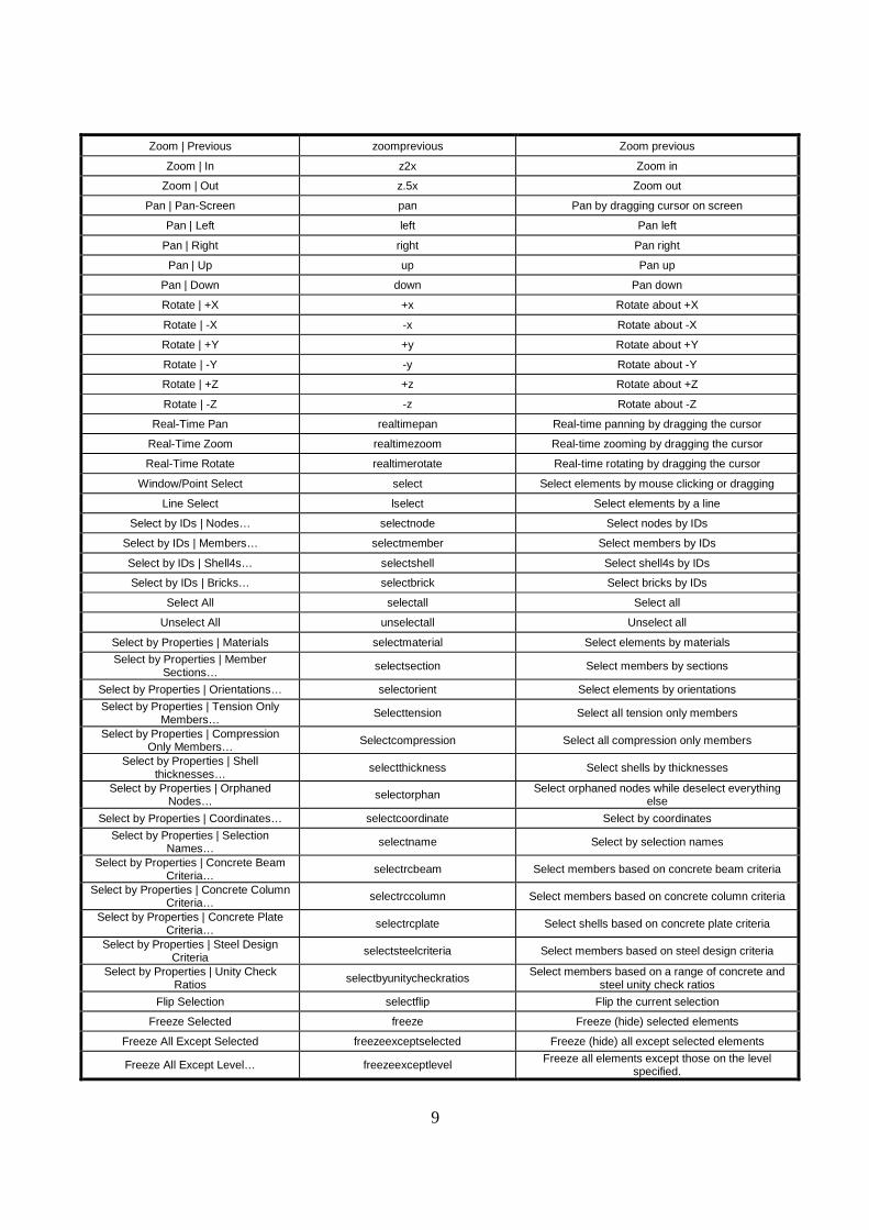
9

Zoom | Previous zoomprevious Zoom previous

Zoom | In z2x Zoom in

Zoom | Out z.5x Zoom out

Pan | Pan-Screen pan Pan by dragging cursor on screen

Pan | Left left Pan left

Pan | Right right Pan right

Pan | Up up Pan up

Pan | Down down Pan down

Rotate | +X +x Rotate about +X

Rotate | -X -x Rotate about -X

Rotate | +Y +y Rotate about +Y

Rotate | -Y -y Rotate about -Y

Rotate | +Z +z Rotate about +Z

Rotate | -Z -z Rotate about -Z

Real-Time Pan realtimepan Real-time panning by dragging the cursor

Real-Time Zoom realtimezoom Real-time zooming by dragging the cursor

Real-Time Rotate realtimerotate Real-time rotating by dragging the cursor

Window/Point Select select Select elements by mouse clicking or dragging

Line Select lselect Select elements by a line

Select by IDs | Nodes… selectnode Select nodes by IDs

Select by IDs | Members… selectmember Select members by IDs

Select by IDs | Shell4s… selectshell Select shell4s by IDs

Select by IDs | Bricks… selectbrick Select bricks by IDs

Select All selectall Select all

Unselect All unselectall Unselect all

Select by Properties | Materials selectmaterial Select elements by materials

Select by Properties | Member Sections… selectsection Select members by sections

Select by Properties | Orientations… selectorient Select elements by orientations

Select by Properties | Tension Only Members…

Selecttension Select all tension only members

Select by Properties | Compression Only Members… Selectcompression Select all compression only members

Select by Properties | Shell thicknesses… selectthickness Select shells by thicknesses

Select by Properties | Orphaned Nodes… selectorphan Select orphaned nodes while deselect everything

else

Select by Properties | Coordinates… selectcoordinate Select by coordinates

Select by Properties | Selection Names… selectname Select by selection names

Select by Properties | Concrete Beam Criteria…

selectrcbeam Select members based on concrete beam criteria

Select by Properties | Concrete Column Criteria… selectrccolumn Select members based on concrete column criteria

Select by Properties | Concrete Plate Criteria… selectrcplate Select shells based on concrete plate criteria

Select by Properties | Steel Design Criteria

selectsteelcriteria Select members based on steel design criteria

Select by Properties | Unity Check Ratios selectbyunitycheckratios

Select members based on a range of concrete and steel unity check ratios

Flip Selection selectflip Flip the current selection

Freeze Selected freeze Freeze (hide) selected elements

Freeze All Except Selected freezeexceptselected Freeze (hide) all except selected elements

Freeze All Except Level… freezeexceptlevel Freeze all elements except those on the level specified.

10

Freeze All Except Plane… freezeexcept Freeze all elements except those on the plane specified.

Thaw thaw Thaw the freezed elements

Load Diagram… loaddiagram View loading Diagram

Annotate… annotate Annotate graphic entities

Query… query Query a node or element info

Distance distance Measure distance between two nodes

Render Options… render Render elements in 3D

Quick Render qrender Quick render

Diaphragm Render renderdiaphragm Render diaphragm

Result Diagram | Shear & Moment Diagram… momentshear Show shear and moment diagram

Result Diagram | Deflection Diagram… deflection Show deflections

Result Diagram | Contour Diagram… contour Show contours

- qcontour Quickly show contours

Result Diagram | Mode Shape… modeshape Show mode shape

Result Diagram | Unity Check unity View design unity check result

Result Diagram | Response Animation animate Animate structural animation

Options | Show Grid showgrid Show or hide drawing grid

Options | Global Axes showaxis Show or hide global axes

Options | Contour Legend showlegend Show or hide contour legend

Options | Comment comment Insert a comment at specified location

Geometry Menu

Materials… material Define or/and assign element materials

Sections… section Define or/assign member sections

Thicknesses… thickness Define or/and assign shell thicknesses

Levels Level Define floor levels

Drawing Grid… grid Generate drawing grid

Object Snap | Snap to 1/2, 1/3…1/9 Points

snap2, 3, …9 Snap to 1/2, 1/3 … 1/9th points on member when drawing nodes, members etc.

Object Snap | Perpendicular Point perpendicular Snap to perpendicular point on member when drawing nodes, members etc.

Clear Snap Points clearsnap Clear all snap options

Draw Node node Draw nodes

Draw Member member Draw members

Draw Shell4 shell Draw shell4s

Draw Brick brick Draw 8-node brick

Quick Draw | Member qmember Draw members by specifying node IDs

Quick Draw | Shell4 qshell Draw shell4s by specifying node IDs

Quick Draw | Brick qbrick Draw bricks by specifying node IDs

Generate | Rectangular Frames… genframe Generate 2D or 3D rectangular frames or continuous

beams

Generate | Cylindrical Frames… gencframe Generate 2D or 3D cylindrical frames

Generate | Rectangular Shell4s… genrectshell Generate shell4s in a rectangle

Generate | Circular Shell4s… gencirshell Generate shell4s in a circle

Generate | Arc Members… genarcmember Generate arc members

Generate | Non-Prismatic Members… gennonprismatic Generate non-prismatic members on selected members

Generate | Nodes from Grid gennodesfromgrid Generate nodes from current grid

Generate | Members by Nodes… genmembersbynodes Generate members by existing nodes

Generate | Shells by Nodes… genshellsbynodes Generate shells by existing nodes

11

Generate | Bricks by Nodes… genbricksbynodes Generate bricks by existing nodes

Element Local Angles… elementangle Assign element local angles

Moment Releases… release Assign moment releases to selected members

Rigid Offset rigidoffset Define and assign rigid offsets to selected members

Tension/Compression Only… tensioncompressiononly Assign tension only or compression only attribute to selected members

Convert Selected Members to Rigid Links rigidlink Convert selected members to rigid links

Element Activation elementactivate Activate or inactivate elements

Supports… support Assign supports to selected nodes

Springs… spring Assign nodal, line or surface springs to selected

nodes, members or shells

Coupled Springs… cspring Assign coupled springs to selected nodes

Diaphragms… diaphragm Define diaphragms

Inclined Rollers inclinedroller Assign inclined rollers to selected nodes

Equal Constraints equalconstraint Assign equal constraints to two nodes

Generic Constraint genericconstraint Assign generic constraints to one or two nodes

Story Drift Nodes driftnodes Assign selected nodes as drift nodes

Loads Menu

Load Cases… loadcase Define load cases

Load Combinations… loadcomb Define load combinations

Nodal Loads… nodalload Assign nodal loads to selected nodes

Point Loads… pointload Assign point forces or moments to selected members

Line Loads… lineload Assign linear forces to selected members

Area Loads… areaload Assign area loads to selected members

Surface Loads… surfaceload Assign surface forces to selected shells

Thermal Loads thermal Assign thermal loads to selected members, shells or bricks

Self Weights… self weight Apply self weight

Self Weight Exclusion selfweightexclude Include or exclude self weight for selected elements

Generate Loads | Fluid Loads… fluidload Generate fluid loads to selected shells

Generate Loads | Pattern Loads... patternload Generate pattern loads to selected members

Generate Loads | Moving Loads... movingload Generate moving loads to selected members

Case-Copy Loads… casecopy Copy loads from one load case to another

Convert Area Loads to Line Loads area2lineload Convert all area loads to line loads

Convert Local Loads to Global Loads local2globalload Convert all local loads to global loads

Additional Masses… mass Assign additional mass or mass moment of inertia to selected nodes

Assign Menu

Support asupport Assign supports continuously

Spring aspring Assign nodal, line or surface springs continuously

Member Properties amember Assign member properties continuously

Shell Properties ashell Assign shell properties continuously

Nodal Load anodalload Assign nodal loads continuously

Point Load apointload Assign point loads continuously

Line Load alineload Assign line loads continuously

Surface Load asurfaceload Assign surface loads continuously

Additional Masses amass Assign additional masses continuously

Convert Inertia Forces to Nodal Forces convertinertiaforces Convert inertia forces from response spectrum

12

analysis to nodal forces

Response Spectra Library spectra Define response spectrum library

Deletion adelete Delete objects continuouly

Input Data Menu

Materials… material Define or/and assign element materials

Sections… section Define or/assign member sections

Thicknesses… thickness Define or/and assign shell thicknesses

Nodes… nodedata Node data sheet

Members… memberdata Member data sheet

Shell4s… shelldata Shell4 data sheet

Bricks… brickdata Brick data sheet

Supports… supportdata Support data sheet

Nodal Springs… nodalspringdata Nodal spring data sheet

Coupled Springs cspringdata Coupled spring data sheet

Line Springs… linespringdata Line spring data sheet

Surface Springs… surfacespringdata Surface (shell4) spring data sheet

Member Releases… releasedata Member release data sheet

Diaphragms… diaphragmdata Diaphragm data sheet

Multi-DOF Constraints multidofdata Multi-DOF constraint data sheet

Load Cases… loadcase Define load cases

Load Combinations… loadcomb Define load combinations

Nodal Loads… nodalloaddata Nodal load data sheet

Point Loads… pointloaddata Member point load data sheet

Line Loads… lineloaddata Member line load data sheet

Area Loads… arealoaddata Member area load data sheet

Surface Loads… surfaceloaddata Shell4 surface load data sheet

Member Thermal Loads mthermaldata Member thermal load data sheet

Shell4 Thermal Loads sthermaldata Shell4 thermal load data sheet

Brick Thermal Loads bthermaldata Brick thermal load data sheet

Self Weights… selfweight Apply self weight

Calculated Masses (Read Only)… calcmassdata Masses calculated from mass load combination

Additional Masses massdata Additional nodal mass data

Story Drift Nodes… driftnodesdata Story Drift nodes data

Convert Inertia Forces to Nodal Forces convertinertiaforces Convert inertia forces from response spectrum

analysis to nodal forces

Response Spectra Library spectra Define response spectrum library

Comments commentdata Comment data

Run Menu

Analysis Options… runoption Set up analysis options

Static Analysis run Run static analysis of the model

Frequency Analysis… frequency Run frequency analysis of the model

Response Spectrum Analysis spectrumanalysis Run response spectrum analysis of the model

Text Report… report Run input or/and output text report

Envelope Report… envelopereport Run envelope report

View Log File viewlog View log file

13

Analysis Result Menu Nodal Displacements… nodaldisplacement Nodal displacements data sheet

Story Drifts… Storydrift Story drift data sheet

Support Reactions… supportreaction Support reaction data sheet

Spring Reactions | Nodal… nodalspringreaction Nodal spring reaction data sheet

Spring Reactions | Coupled… cspringreaction Coupled spring reaction data sheet

Spring Reactions | Line… linespringreaction Line spring reaction data sheet

Spring Reactions | Surface… surfacespringreaction Surface (shell4) spring reaction data sheet

Multi-DOF Constraint Forces & Moments constraintforce Multi-DOF constraint forces & moments data sheet

Member End Forces & Moments… memberendforcemoment Member end forces and moments da

Member Segmental Results… msegmentalforcemoment Member segmental force, moment and deflection

Shell4 Forces & Moments… shellforcemoment Shell4 internal force and moment data sheet

Shell4 Principal Forces & Moments… sprincipalforcemoment Shell4 principal force and moment data sheet

Shell4 Stresses [Top]… shelltopstress Shell4 top stress data sheet

Shell4 Stresses [Bottom]… shellbottomstress Shell4 bottom stress data sheet

Shell4 Principal Stresses… shellprincipalstress Shell4 top/bottom principal stress data sheet

Shell4 Nodal Resultants… shellnodalresultant Show shell4 nodal resultants

Brick Stresses… brickstress Brick stress data sheet

Brick Principal Stresses… brickprincipalstress Brick principal stress data sheet

Envelope | Nodal Displacements nodaldisplacementenvelope Nodal displacement envelope

Envelope | Support Reactions supportreactionenvelope Support reaction envelope

Envelope | Member Segemental Results msegmentalforcemomentenvelope Member segmental envelope

Eigenvalues… eigenvalue Eigenvaule spreadsheet

Eigenvectors… eigenvector Eigenvector spreadsheet

Mode Participation Factors participationfactors Mode participation factors spreadsheet

Modal Displacements | Modal Displacements (SX) modaldisplacementsx Modal displacements spreadsheet in global X

direction Modal Displacements | Modal

Displacements (SY) modaldisplacementsy Modal displacements spreadsheet in global Y

direction Modal Displacements | Modal

Displacements (SZ) modaldisplacementsz Modal displacements spreadsheet in global Z direction

Inertia Forces | Inertia Forces (SX) inertiaforcesx Inertia forces spreadsheet in global X direction

Inertia Forces | Inertia Forces (SY) inertiaforcesy Inertia forces spreadsheet in global Y direction

Inertia Forces | Inertia Forces (SZ) inertiaforcesz Inertia forces spreadsheet in global Z direction

Modal Combinations | Nodal Displacements

modalcombodisplacements Nodal displacements for modal combinations

Modal Combinations | Support Reactions modalcombsupportreactions Support reactions for modal combinations

Modal Combinations | Nodal Spring Reactions modalcombcspringreactions Coupled spring reactions for modal combinations

Modal Combinations | Coupled Spring Reactions modalcombnodalspringreactions Nodal spring reactions for modal combinations

Modal Combinations | Line Spring Reactions modalcomblinespringreactions Line spring reactions for modal combinations

Modal Combinations | Surface Spring Reactions

modalcombsurfacespringreactions Surface spring reactions for modal combinations

Modal Combinations | Multi-DOF Constraint Forces & Moments modalcombconstraintforce Multi-DOF constraint forces & moments modal

combinations Modal Combinations | Member End

Forces & Moments modalcombmemberendforcesmoments Member end forces and moments for modal

combinations Modal Combinations | Member

Segmental Results modalcombmembersegmentalresults Member segmental results for modal combinations

Modal Combinations | Shell4 Forces & Moments modalcombshell4forcesmoments Shell4 forces and moments for modal combinations

Modal Combinations | Brick Stresses modalcombbrickstresses Brick stresses for modal combinations

14

RC Design Menu

RC Materials… rcmaterial Define RC materials

Design Criteria | Model Design Criteria… rcmodel Set RC model design options

Design Criteria | Beam Design Criteria… rcbeam Define or/and assign RC beam design criteria

Design Criteria | Column Design Criteria… rccolumn Define or/and assign RC column design criteria

Design Criteria | Plate Design Criteria… rcplate Define or/and assign RC plate design criteria

Design Criteria | Exclude Elements… rcexclude Exclude or include selected elements from RC

design

Cracking Factors… crackingfactor Assign element cracking factors

Assign | Beam Design Properties acbeam Assign concrete beam design properties to selected

members

Assign | Column Design Properties accolumn Assign concrete column design properties to selected members

Assign | Plate Design Properties acplate Assign concrete plate design properties to selected

members

Design Input | RC Member Input… rcmemberdata RC member input data sheet

Design Input | RC Plate Input… rcplatedata RC plate input data sheet

Perform Design rcrun Perform concrete design

Design Results | RC Analysis Envelope… rcenvelope RC member envelope moment and shear data sheet

Design Results | RC Beam Results… rcbeamresult Show RC beam flexural design results

Design Results | RC Column Results… rccolresult Show RC column axial-flexural design results

Design Results | RC Sections… rcsection RC Column sections

Design Results | Flexural/Axial Interaction | P-Mx(+)…

pmx+ P-Mx (+) interaction table

Design Results | Flexural/Axial Interaction | P-Mx(-)…

pmx- P-Mx (-) interaction table

Design Results | Flexural/Axial Interaction | P-My(+)…

pmy+ P-My (+) interaction table

Design Results | Flexural/Axial Interaction | P-My(-)…

pmy- P-My (-) interaction table

Design Results | Flexural/Axial Interaction | P-Mx-My…

pmxmy P-Mx-My interaction table

Design Results | Flexural/Axial Interaction |

Print Diagrams… interactiondiagram Print concrete column interaction diagrams

Design Results | Member Shear Design… rcshearresult Show RC member shear design result

Design Results | Wood-Armer Moments…

woodarmer Show Wood-Armer Moments

Design Results | RC Plate Results… rcplateresult Show RC plate results

Diagrams | RC Member Envelope Diagram… rcenvelopediagram Show member envelop and capacity diagrams

Diagrams | RC Plate Envelope Contour… rcenvelopecontour Show or hide plate envelope contour

RC Report… rcreport Run concrete report

RC Tools | Rebar Database… rebardatabase Show rebar database

RC Tools | K-Calculator… kfactor Compute K Factor

RC Tools | Quick R-Beam Flexural Design… rcrectas Compute flexural reinforcement for rectangular beam

RC Tools | Quick T-Beam Flexural Design… rcteeas Compute flexural reinforcement for tee beam

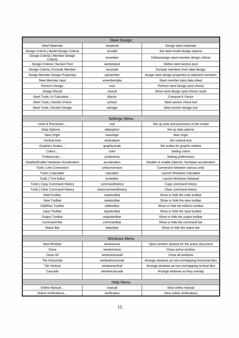
15

Steel Design Steel Materials smaterial Design steel materials

Design Criteria | Model Design Criteria smodel Set steel model design options

Design Criteria | Member Design Criteria smember Define/assign steel member design criteria

Design Criteria | Section Pool sectionpool Define steel section pool

Design Criteria | Exclude Member sexclude Exclude members from steel design

Assign Member Design Properties asmember Assign steel design properties to selected members

Steel Member Input smemberdata Steel member input data sheet

Perform Design srun Perform steel design (and check)

Design Result sresult Show steel design (and check) result

Steel Tools | K-Calculator… kfactor Compute K Factor

Steel Tools | Section Check scheck Steel section check tool

Steel Tools | Section Design sdesign Steel section design tool

Settings Menu

Units & Precisions… unit Set up units and precisions in the model

Data Options… dataoption Set up data options

New Origin neworigin New origin

Vertical Axis verticalaxis Set vertical axis

Graphics Scales… graphicscale Set scales for graphic entities

Colors… color Setting colors

Preferences… preference Setting preferences

Disable/Enable Hardware Acceleration acceleration Disable or enable OpenGL hardware acceleration

Tools | Unit Conversion unitconversion Conversion between various units

Tools | Calculator calculator Launch Windows Calculator

Tools | Text Editor texteditor Launch Windows Notepad

Tools | Copy Command History commandhistory Copy command history

Tools | Clear Command History clearcommandhistory Clear command history

MainToolbar maintoolbar Show or hide the main toolbar

View Toolbar viewtoolbar Show or hide the view toolbar

Edit/Run Toolbar edittoolbar Show or hide the edit/run toolbar

Input Toolbar inputtoolbar Show or hide the input toolbar

Output Toolbar outputtoolbar Show or hide the output toolbar

Command Bar commandbar Show or hide the command bar

Status Bar statusbar Show or hide the status bar

Windows Menu

New Window windownew Open another window for the active document

Close windowclose Close active window

Close All windowcloseall Close all windows

Tile Horizontal windowhorizontal Arrange windows as non-overlapping horizontal tiles

Tile Vertical windowvertical Arrange windows as non-overlapping vertical tiles

Cascade windowcascade Arrange windows so they overlap

Help Menu

Online Manual… manual View online manual

Online Verifications… verification View online verifications

16

Command List… commandlist View command list

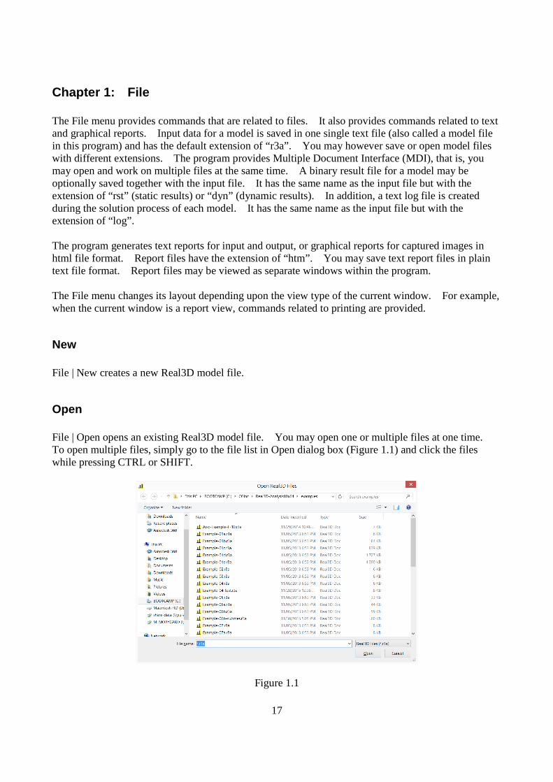
17

Chapter 1: File The File menu provides commands that are related to files. It also provides commands related to text and graphical reports. Input data for a model is saved in one single text file (also called a model file in this program) and has the default extension of “r3a”. You may however save or open model files with different extensions. The program provides Multiple Document Interface (MDI), that is, you may open and work on multiple files at the same time. A binary result file for a model may be optionally saved together with the input file. It has the same name as the input file but with the extension of “rst” (static results) or “dyn” (dynamic results). In addition, a text log file is created during the solution process of each model. It has the same name as the input file but with the extension of “log”. The program generates text reports for input and output, or graphical reports for captured images in html file format. Report files have the extension of “htm”. You may save text report files in plain text file format. Report files may be viewed as separate windows within the program. The File menu changes its layout depending upon the view type of the current window. For example, when the current window is a report view, commands related to printing are provided.

New File | New creates a new Real3D model file.

Open File | Open opens an existing Real3D model file. You may open one or multiple files at one time. To open multiple files, simply go to the file list in Open dialog box (Figure 1.1) and click the files while pressing CTRL or SHIFT.

Figure 1.1

18

Multiple Document Interface (MDI) makes it easy for you to share data and compare results between different models. Multiple windows or views may be associated with a single file. These windows may have different display settings with respect to zooming, panning, displaying or hiding various structural entities, annotations, etc. For example, you may have one window for geometry, another window for loading diagrams, and yet another window for moment and shear diagrams.

Close When the current window is a model view, File | Close closes the active Real3D model file. You will be prompted to save the document if changes have been made since it was last saved. You may close all opened documents without exiting the program. When the current window is a report view, File | Close closes the report window instead.

Save When the current window is a model view, File | Save saves the model. If the model has not been saved before, the Save As dialog box will be displayed prompting you to enter a file name. When the current window is a report view, File | Save saves the report file.

Save As When the current window is a model view, File | Save As saves the model under a different name. It may be used if you have never saved the model or if you want to keep the original file. When the current window is a report view, File | Save As saves the report file under a different name. For example, you may save the text report file in a plain text file format instead of the default html file format.

Save All File | Save All will save all the documents currently opened. If a model has not been saved before, the Save As dialog box will be displayed prompting you to enter a file name.

Append File File | Append File command allows you to append data from an existing Real3D input file to the current model. The following data will always be appended: materials, sections, thicknesses, geometry (nodes, members, shells or bricks), boundary conditions (supports, springs, moment releases, diaphragms etc.), concrete beam design criteria, concrete column design criteria and concrete plate design criteria. Loads, load cases and load combinations may be optionally appended. Other data such as analysis options and concrete model design criteria will not be appended. The input file does

19

not need to use the same unit system as that of the current model. The program performs the unit conversion automatically. It is important to point out that you should NOT use the default material, section or thickness in the input file as this could cause data conflicts if corresponding properties do not match those of the current model. Data conflict may also occur if materials, sections, thicknesses, load combinations etc. in the input file already exists in the current model. The program gives you warnings if such conditions occur. You should examine these warnings carefully and make corrections if necessary. The following dialog box (Figure 1.2) gives you more options for Append File command. The insertion point will add an offset to the nodal coordinates in the input file. You also have the option to give distinct node and element numbering for the appended data.

Figure 1.2

Import from DXF File | Import from DXF imports geometry data from a DXF file to the program. DXF stands for Drawing eXchange Format and is widely supported by many CAD and structural analysis programs. Real3D converts all lines into members and 3D faces to shells. Nodes are created as needed. The command prompts you with a file selection dialog box. After selecting a DXF file, you are then prompted with the following dialog box (Figure 1.3): You have the option to select length unit in the DXF file. You may also specify an insertion point at which the imported geometry will be inserted. The program merges nodes and elements automatically after the importing. You may run this command as many times as needed.

20

Figure 1.3

Import from SAP2000 .s2k File | Import from SAP2000 .s2k offers limited support to import data from a SAP2000 (V15 or above) .s2k file to the program. You will be prompted with the following message box:

Currently, Real3D reads the following sections in the .s2k file:

PROGRAM_CONTROL MATERIAL_PROPERTIES_02_BASIC_MECHANICAL_PROPERTIES FRAME_SECTION_PROPERTIES_01_GENERAL AREA_SECTION_PROPERTIES JOINT_PATTERN_ASSIGNMENTS LOAD_PATTERN_DEFINITIONS JOINT_COORDINATES JOINT_RESTRAINT_ASSIGNMENTS JOINT_SPRING_ASSIGNMENTS_1_UNCOUPLED CONNECTIVITY_FRAME FRAME_SECTION_ASSIGNMENTS FRAME_LOCAL_AXES_ASSIGNMENTS_1_TYPICAL CONNECTIVITY_AREA JOINT_LOADS_FORCE AREA_SECTION_ASSIGNMENTS FRAME_LOADS_POINT FRAME_LOADS_DISTRIBUTED AREA_LOADS_UNIFORM AREA_LOADS_SURFACE_PRESSURE

Export to DXF

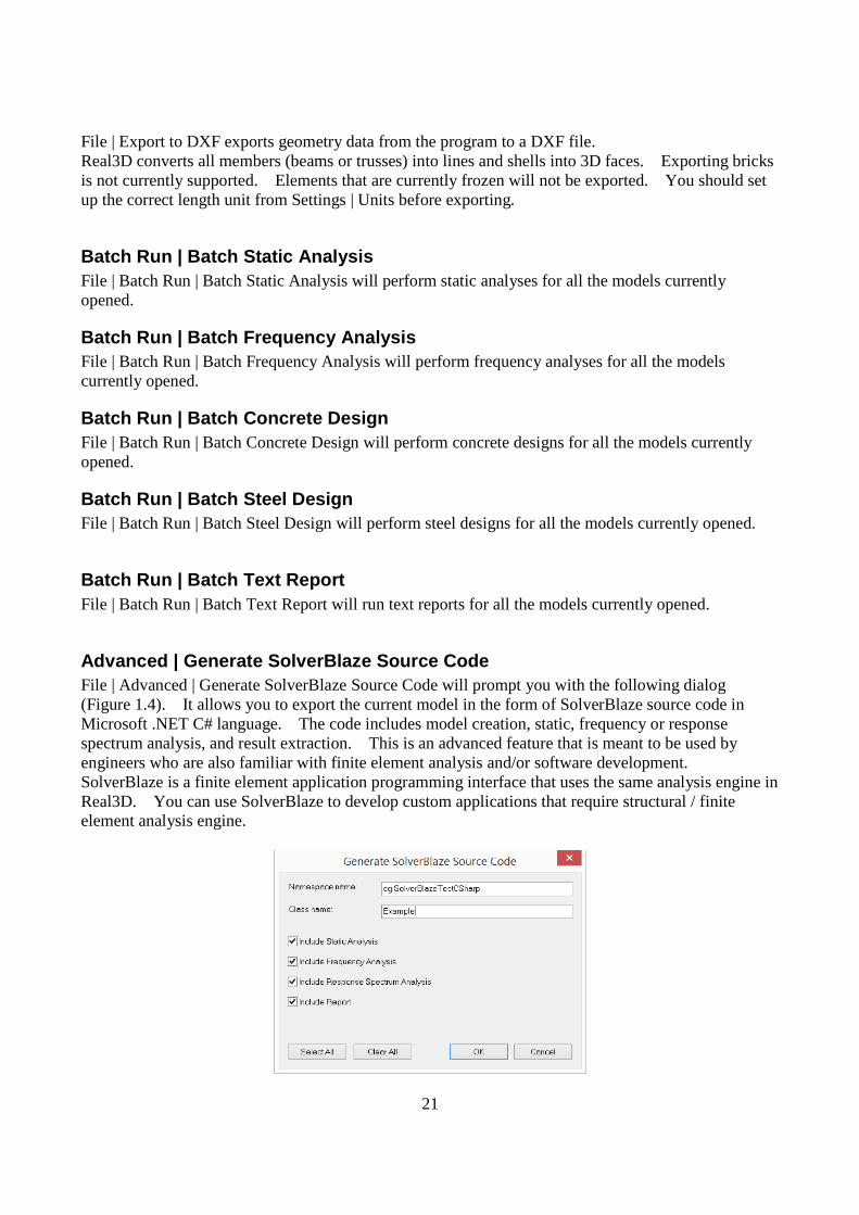
21

File | Export to DXF exports geometry data from the program to a DXF file. Real3D converts all members (beams or trusses) into lines and shells into 3D faces. Exporting bricks is not currently supported. Elements that are currently frozen will not be exported. You should set up the correct length unit from Settings | Units before exporting.

Batch Run | Batch Static Analysis File | Batch Run | Batch Static Analysis will perform static analyses for all the models currently opened.

Batch Run | Batch Frequency Analysis File | Batch Run | Batch Frequency Analysis will perform frequency analyses for all the models currently opened.

Batch Run | Batch Concrete Design File | Batch Run | Batch Concrete Design will perform concrete designs for all the models currently opened.

Batch Run | Batch Steel Design File | Batch Run | Batch Steel Design will perform steel designs for all the models currently opened.

Batch Run | Batch Text Report File | Batch Run | Batch Text Report will run text reports for all the models currently opened.

Advanced | Generate SolverBlaze Source Code File | Advanced | Generate SolverBlaze Source Code will prompt you with the following dialog (Figure 1.4). It allows you to export the current model in the form of SolverBlaze source code in Microsoft .NET C# language. The code includes model creation, static, frequency or response spectrum analysis, and result extraction. This is an advanced feature that is meant to be used by engineers who are also familiar with finite element analysis and/or software development. SolverBlaze is a finite element application programming interface that uses the same analysis engine in Real3D. You can use SolverBlaze to develop custom applications that require structural / finite element analysis engine.

22

Figure 1.4

Print Setup (Model View) File | Print Setup allows you to set up the page layout (Figure 1.5) before printing model views, captured images or concrete column interaction diagrams.

Figure 1.5

Print Setup (Report View) File | Print Setup allows you to set up the printing page layout such as margins and printing orientation before you print a text or graphical report (Figure 1.6). If you are to print a graphical report, you should set the printing orientation consistent with the setting of table width and height when you run File | View/Print Images for that report.

23

Figure 1.6

Print Preview (Report View) File | Print Preview allows you to preview the printing layout before printing a text or graphical report. It is always a good idea to run this command before the printing to make sure the report will be printed properly.

Print (Report View) File | Print prints a text or graphical report. It is recommended that you run File | Print Preview before running this command.

Print Current View File | Print Current View allows you to preview and print the current model view.

Capture Images | Capture Current Image File | Capture Images | Capture Current Image captures the current graphical view as it appears on screen. You may capture up to 100 images of the same view or different views. Captured images are saved in JPG format under the same directory as the model file. If you intend to print these images, they should all be approximately the same size. The width and height of the current window are displayed on the right-most pane of the status bar.

Capture Images | Delete All Images File | Capture Images | Delete All Images deletes all captured images. Since image files are usually large, you may want to delete these files when they are no longer needed.

Capture Images | Print Captured Images File | Capture Images | Print Captured Images allows you to preview and print the captured images. You must have captured one or more images already before running this command.

General Information File | General Information prompts you with the following dialog box (Figure 1.7). You may enter a model name, your company name, your name and a description about the model (up to 1020 characters long).

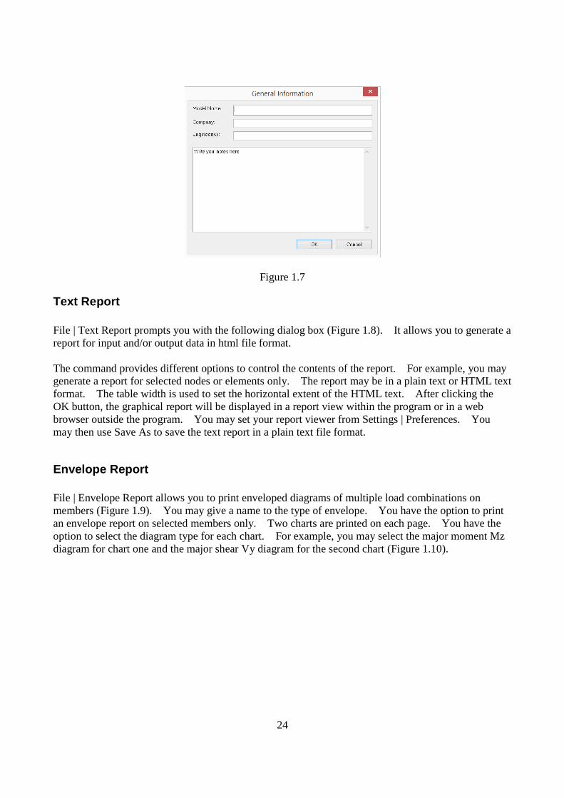
24

Figure 1.7

Text Report File | Text Report prompts you with the following dialog box (Figure 1.8). It allows you to generate a report for input and/or output data in html file format. The command provides different options to control the contents of the report. For example, you may generate a report for selected nodes or elements only. The report may be in a plain text or HTML text format. The table width is used to set the horizontal extent of the HTML text. After clicking the OK button, the graphical report will be displayed in a report view within the program or in a web browser outside the program. You may set your report viewer from Settings | Preferences. You may then use Save As to save the text report in a plain text file format.

Envelope Report File | Envelope Report allows you to print enveloped diagrams of multiple load combinations on members (Figure 1.9). You may give a name to the type of envelope. You have the option to print an envelope report on selected members only. Two charts are printed on each page. You have the option to select the diagram type for each chart. For example, you may select the major moment Mz diagram for chart one and the major shear Vy diagram for the second chart (Figure 1.10).

25

Figure 1.8

Figure 1.9

26

Figure 1.10

27

Statistics File | Statistics displays the key statistics about the model (Figure 1.11).

Figure 1.11

View Log File File | View Log File allows you to view the log file generated during the solution process

Open Containing Folder File | Open Containing Folder allows you to open the folder that contains the current model file.

28

Chapter 2: Edit The Edit main menu provides commands to edit or modify the model.

Undo Edit | Undo undoes the previous structural command. By default, you may undo up to 10 levels. You may set a different number of undo levels by running Settings | Data Options. Non-structural commands such as zooming or panning may not be undone. More undo levels requires more computer memory.

Redo Edit | Redo reverses the previous undo command.

Lock Model Edit | Lock Model locks the model so that you cannot modify it. You may still run non-structural commands such as zooming and panning while the model is locked. The model may be automatically locked after an analysis is performed successfully. To do that, just run Settings | Preferences.

Duplicate Edit | Duplicate prompts you with the following dialog box (Figure 2.1). It allows you make one copy of the selected parts of a model to a different location. You may specify copy distances along the X, Y or Z directions. Nodal or element dependents (except loads) are copied together with their parents automatically. For example, when a member is copied, moment releases on that member are copied also. You have the option to copy the loads attached to the selected nodes or elements. You have the option to automatically merge nodes and elements after copying. You should check this option unless duplicate nodes are explicitly permitted.

Figure 2.1

29

Array Edit | Array prompts you with the following dialog box (Figure 2.2). It allows you make one or more copy of the selected parts of a model to a different location. You may specify the step size along the X, Y or Z directions. Nodal or element dependents (except loads) are copied together with their parents automatically. For example, when a member is copied, moment releases on that member are copied also. You have the option to copy the loads attached to the selected nodes or elements. You have the option to automatically merge nodes and elements after copying. You should check this option unless duplicate nodes are explicitly permitted.

Figure 2.2

Mirror Edit | Mirror prompts you with the following dialog box (Figure 2.3). It allows you make one mirror copy of the selected parts of a model about XY, YZ or XZ plane. Nodal or element dependents (except loads) are mirrored together with their parents automatically. For example, when a member is mirrored, moment releases on that member are mirrored also. You have the option to copy (not mirror) the loads attached to the selected nodes or elements. You have the option to automatically merge nodes and elements after mirroring. You should check this option unless duplicate nodes are explicitly permitted. You may also need to reverse brick node ordering after mirroring in order to prevent negative element diagonal stiffness terms.

Figure 2.3

30

Move Edit | Move prompts you with the above dialog box (Figure 2.4). It lets you move selected parts of a model to a different location. You may specify move distances along the X, Y or Z directions. Nodal or element dependents such as loads are moved together with selected nodes or elements automatically. You have the option to automatically merge nodes and elements after moving. You should check this option unless duplicate nodes are explicitly permitted.

Figure 2.4

Rotate Edit | Rotate prompts you with the following dialog box (Figure 2.5). It lets you rotate selected parts of a model by an angle about one of the global axes. Nodal or element dependents such as loads are moved together with the elements. You have the option to automatically merge nodes and elements after rotating. You should check this option unless duplicate nodes are explicitly permitted.

Figure 2.5

Figure 2.6

Scale

31

Edit | Scale prompts you with the above dialog box (Figure 2.6). It lets you scale selected parts of a model in the X, Y or Z directions. You may specify the coordinates of a base point and scales for the three global directions. The following formula is used to perform the scaling in the program. Xnew = Xbase + (Xold - Xbase) * scale Where Xnew represents the nodal coordinates after scaling, Xold represents the nodal coordinates before scaling and Xbase represents coordinates of the base point.

Delete Edit | Delete prompts you with the following dialog box (Figure 2.7). It allows you to delete selected nodes or elements or their dependents. Loads are deleted based on their visibilities in the model view. Dependents such as loads will be deleted if their parent nodes or elements are deleted.

Figure 2.7

Extrude | Extrude Nodes to Members Edit | Extrude | Extrude Nodes to Members prompts you with the following dialog box (Figure 2.8). It generates a series of members by extruding selected nodes along a global direction. You may specify a distance list and an extrusion direction for the generation of beams. The distance list is a comma separated list that specifies multiple distances. For example, a distance list of “12,2@14,3@10” will generate distances of 12, 14, 14, 10, 10 and 10 in length units. You have the option to automatically merge nodes and elements after extrusion. You should check this option unless duplicate nodes are explicitly permitted. The following members in Figure 2.9 are generated by extruding one node (the first node) using the input from Figure 2.8.

32

Figure 2.8

Figure 2.9

Extrude | Extrude Members to Shell4s Edit | Extrude | Extrude Members to Shell4s prompts you with the following dialog box (Figure 2.10). It generates a series of shells by extruding selected members along a global direction. You may specify a distance list and an extrusion direction for the generation of shells. The extrusion direction must not be parallel to the selected members. You have the option to automatically merge nodes and elements after extrusion. You should check this option unless duplicate nodes are explicitly permitted. You also have the option to automatically delete selected members after the extrusion.

Figure 2.10

In the following two figures, shells in Figure 2.12 are generated by extruding members in Figure 2.11 using the input from Figure 2.10.

members used for extruding

Figure 2.11

shells generated

Figure 2.12

33

Extrude | Extrude Shell4s to Bricks Edit | Extrude | Extrude Shell4s to Bricks prompts you with the following dialog box (Figure 2.13). It generates a series of bricks by extruding selected shells along a global direction. You may specify a distance list and an extrusion direction for the generation of shells. The extrusion direction must not be parallel to the selected shells. You have the option to automatically merge nodes and elements after extrusion. You should check this option unless duplicate nodes are explicitly permitted. You also have the option to automatically delete selected shells after the extrusion.

Figure 2.13

In the following two figures, bricks in Figure 2.15 are generated by extruding shells in Figure 2.14 using the input from Figure 2.13.

shells used for extruding

Figure 2.14

bricks generated

Figure 2.15

Revolve | Revolve Members to Shell4s Edit | Revolve | Revolve Members to Shell4s prompts you with the following dialog box (Figure 2.16). It generates a series of shells by revolving selected members (in XY plane) about the global Y axis. You may specify the number of segments, start and end angles (measured from X-Axis) for revolving. The program will merge nodes automatically. You have the option to automatically delete the selected members after revolving.

34

Figure 2.16 For example, in the following two figures, shells in Figure 2.18 are generated by revolving members in Figure 2.17 using the input in Figure 2.16.

members used for revolving

Figure 2.17

shells generated

Figure 2.18

Revolve | Revolve Shell4s to Bricks Edit | Revolve | Revolve Shell4s to Bricks prompts you with the following dialog box (Figure 2.19). It generates a series of bricks by revolving selected shell4s about the global Y axis. You may specify the number of segments, start and end angles for revolving. The program will merge nodes automatically. You have the option to automatically delete the selected shells after revolving.

35

Figure 2.19 In the following two figures, bricks in Figure 2.21 are generated by revolving shells in Figure 2.20 using the input from Figure 2.19. Bricks are rendered in the figure.

shells used for revolving

Figure 2.20

bricks generated

Figure 2.21

Split Members Edit | Split Members prompts you with the following dialog box (Figure 2.22). It allows you to divide selected members by specifying 2 or more segments of equal length or by providing a distance list. Loads on the original members are assigned automatically to the generated members after splitting. You have the option to automatically merge nodes and elements after splitting.

36

Figure 2.22 In the following two figures, members in Figure 2.24 are generated by splitting members in Figure 2.23 using the input from Figure 2.22

members before splitting

Figure 2.23

members after splitting

Figure 2.24

Sub-Mesh Shell4s Edit | Sub-Mesh Shell4s prompts you with the following dialog box (Figure 2.25). It allows you to sub-mesh selected shells by specifying 2 or more segments along sides 1-2 & 4-3 and sides 2-3 & 1-4. Loads on the original shells are assigned automatically to the generated shells after sub-meshing. You have the option to merge nodes and elements after sub-meshing. You should check this option unless duplicate nodes are explicitly permitted.

Figure 2.25

37

In the following two figures, shells in Figure 2.27 are generated by sub-meshing shells in Figure 2.26 using the input from Figure 2.25.

shells before sub-meshing

Figure 2.26

shells after sub-meshing

Figure 2.27

Insert Nodes at Intersections of Selected Members Edit | Insert Nodes at Intersections of Selected Members allows you to insert nodes at all intersections of the selected members. The newly created nodes are likely isolated (orphaned) nodes, meaning they are not attached to intersecting members. Generally speaking, you should explode the members at these nodes. The program prompts you to do so at the end of this command.

Explode Selected Members at Nodes Edit | Explode Selected Members at Nodes allows you to split selected members at nodes which are located on but are not connected to these members. Consider the following three figures: Figure 2.28 shows a shell with edge members on four sides; Figure 2.29 shows shells generated by sub-meshing (2x2) the shell on the left figure; Figure 2.30 shows members generated by exploding members at nodes. Notice in Figure 2.29, the middle nodes on the edge are on but not connected to the members. The figures are rendered using the command View | Render, with the rendering ratio of 80% for both members and shells.

Figure 2.28

Figure 2.29

Figure 2.30

Re-Number | Auto Number All Nodes

38

Edit | Re-Number | Auto Number All Nodes prompts you with the following dialog box (Figure 2.31). It allows you to re-number all nodes sequentially based on nodal coordinates.

Re-Number | Re-Number Selected Nodes Edit | Re-Number | Re-Number Selected Nodes prompts you with the following dialog box (Figure 2.32). It allows you to re-number selected nodes based on the following two modes: a). Increment each selected node number by a delta (may be positive or negative). For example, if we have selected node numbers 2, 5, 8 and a delta of 2, the new node numbers will be 4, 7, and 10. b). Renumber each selected node from a new start number (must be positive) and a step (may be positive or negative). For example, if we have selected node numbers 2, 5, 8, a new start number of 1000 and a step of 2, the new node numbers will be 1000, 1002, 1004. If renumbering is successful, nodal dependents such as loads, masses and springs will be renumbered automatically. The renumbering will be undone automatically if any errors are encountered.

Re-Number | Re-Number Selected Members

Re-Number | Re-Number Selected Shell4s

Re-Number | Re-Number Selected Bricks Edit | Re-Number | Re-Number Members, Shell4s and Bricks commands are similar to Re-Number Nodes and are not repeated here.

Figure 2.31

Figure 2.32

Switch Coordinates Edit | Switch Coordinates prompts you with the following dialog box (Figure 2.33). It allows you to switch the X and Z, or the Y and Z coordinates of the selected nodes. For example, you may generate a floor system on the XY (vertical) plane and then switch coordinates to place the floor on the XZ (horizontal) plane.

39

Figure 2.33

Reverse Node Order for Selected Elements Edit | Reverse Node Order for Selected Elements allows you to reverse the nodes’ order for selected elements. For members and shells, this command in effect changes their local coordinate systems. For bricks, this command may be used to rectify a wrong nodal ordering which results in negative diagonals in element stiffness. It is important to point out that dependents on the elements are not reversed or changed accordingly. After running this command, you should check on these dependents such as loads and moment releases on members, loads on shells, etc.

Merge All Nodes & Elements Edit | Merge All Nodes & Elements merges all nodes that are located within a distance tolerance between two or more nodes, and merges all elements that share the same nodes. You may set the distance tolerance using the command Settings | Data Options.

Remove All Orphaned Nodes Edit | Remove All Orphaned Nodes removes all nodes that are not connected to any elements. Orphaned nodes make the model unstable and should be removed prior to solution (unless they have multi-DOF constraints on them).

Element Local Angle Edit | Element Local Angle prompts you with the above dialog box (Figure 2.34). It allows you to assign local angles to the selected members and/or shells. The element local angle is used to change the element local coordinate system.

40

Figure 2.34

Match Local x-Axes for Shells Edit | Match Local x-Axes for Shells prompts you with the dialog box below (Figure 2.35). It allows you to match local x-Axes of the selected shells with that of a source shell specified in the dialog. The end result is the automatic assignment of local angles to the selected shells. This command may be useful in situations where rectangular and non-rectangular shells are mixed. Please note the default local x-axes are different for rectangular and non-rectangular shells (see Coordinate Systems chapter in Technical Issues of this manual for details).

Figure 2.35

3-Point Member Orientation Edit | 3-Point Member Orientation prompts you with the dialog box below (Figure 2.36). It allows you to auto-calculate and assign a local angle to each of the selected members such that its local z axis is perpendicular to the plane formed by the two member end points and the 3rd point defined here. The local x axis stays the same. The local y axis is determined by the local x and z axes using right hand rule. This command can be useful for some models such as a dome where member webs are in plane with the member ends and the center of the sphere.

Figure 2.36

41

Tension/Compression Only Edit | Tension/Compression Only prompts you with the dialog box below (Figure 2.37). It allows you to assign nonlinearity (linear, tension only or compression only) to the selected members. The member stiffness will be ignored if a tension only member is subjected to compressive forces or if a compression only member is subjected to tensile forces. The presence of tension or compression members makes the model nonlinear and iterative solution is required for each load combination.

Figure 2.37

Convert Selected Members to Rigid Links The Edit | Convert Selected Members to Rigid Links will convert the selected members to rigid links.

Self Weight Exclusion Edit | Self Weight Exclusion prompts you with the following dialog box (Figure 2.38). It allows you to exclude self weight for the selected elements. You can view/edit the self weight exclusion from menu Input Data | Members, Shell4s or Bricks. To include self weight, you also need to set the self weight multiplier from Loads | Self Weights.

Figure 2.38

Element Activation

42

Edit | Element Activation prompts you with the following dialog box (Figure 2.39). It allows you to activate or inactivate the selected elements. You can view/edit the element activation from menu Input Data | Members, Shell4s or Bricks.

Figure 2.39

Clear | Clear Undo & Redo Edit | Clear | Clear Undo & Redo clears the undo/redo buffer, thus frees up computer memory. It is a good idea to run this command before the solution so that more memory may be committed to the solver.

Clear | Clear Results Edit | Clear | Clear Results clears all results from computer memory. You need to re-solve the model to obtain new results.

Clear | Clear Everything Edit | Clear | Clear Everything clears all input and output (results) data from computer memory. You should think twice before running this command.

43

Chapter 3: View The View menu provides commands to graphically view inputs such as geometry and loading; perform selections by various methods; and display outputs such as shear and moment diagrams for members, and contours for shells and bricks.

Redraw View | Redraw regenerates and redraws all graphics in the model view.

Restore Model View | Restore restores original settings for the model view. These settings include zooming = 1.0, panning = 0, rotations = 0s.

Preset Views You may place the model view in a preset orientation by selecting one of these commands (Figure 3.1).

Front Back Left Right

Top Bottom Isometric

Figure 3.1

Named Views View | Named Views allows you to save the current view settings such as zooming factor, panning distance or rotation angles so that you may recall this view later on.

44

Named Selections View | Named Selections prompts you with the following dialog box (Figure 3.2). It allows you to save the currently selected items to a name. You may use the command View | Select by Properties | Selection Names to recall the previously saved named selections. This command is very useful to group related items.

Figure 3.2

Zoom | Zoom Extent View | Zoom | Zoom Extent displays the entire model in the view.

Zoom | Zoom Window View | Zoom | Zoom Window zooms in on a specific part of the model by clicking and dragging the left mouse button. The command remains in effect until another command is selected, the right mouse button is clicked, or ESC is pressed.

Zoom | Zoom Object View | Zoom | Zoom Object zooms in on a specific node, member, shell or brick. The command remains in effect until another command is selected, the right mouse button is clicked, or ESC is pressed.

Zoom | Zoom Previous

45

View | Zoom | Zoom Previous lets you zoom back to the previous view. You may use this command after you zoom in or pan to view a portion of your model in greater detail.

Zoom | Zoom In View | Zoom | Zoom In zooms in on the model by a preset factor (1.25). You may run this command by pressing CTRL+UP arrow or CTRL+RIGHT arrow.

Zoom | Zoom Out View | Zoom | Zoom Out zooms out on the model by a preset factor (1.25). You may run this command by pressing CTRL+DOWN arrow or CTRL+LEFT.

Pan | Pan Screen View | Pan | Pan Screen pans (moves) the model by clicking and dragging the left mouse button. The command remains in effect until another command is selected, the right mouse button is clicked, or ESC is pressed.

Pan | Left View | Pan | Left pans the model to the left by a preset screen distance. You may run this command by pressing CTRL+LEFT arrow.

Pan | Right View | Pan | Right pans the model to the right by a preset screen distance. You may run this command by pressing CTRL+RIGHT arrow.

Pan | Up View | Pan | Up pans the model to the top by a preset screen distance. You may run this command by pressing CTRL+UP arrow.

Pan | Down View | Pan | Down pans the model to the bottom by a preset screen distance. You may run this command by pressing CTRL+DOWN arrow.

46

Rotate | +X View | Rotate | +X rotates the model view about X by a preset positive angle (5 degrees). You may run this command by pressing SHIFT+DOWN arrow.

Rotate | -X View | Rotate | -X rotates the model view about X by a preset negative angle (5 degrees). You may run this command by pressing SHIFT+UP arrow.

Rotate | +Y View | Rotate | +Y rotates the model view about Y by a preset positive angle (5 degrees). You may run this command by pressing SHIFT+RIGHT arrow.

Rotate | -Y View | Rotate | -Y rotates the model view about Y by a preset negative angle (5 degrees). You may run this command by pressing SHIFT+LEFT arrow.

Rotate | +Z View | Rotate | +Z rotates the model view about Z by a preset positive angle (5 degrees). You may run this command by pressing CTRL+SHIFT+UP arrow or CTRL+SHIFT+RIGHT arrow

Rotate | -Z View | Rotate | -Z rotates the model view about Z by a preset negative angle (5 degrees). You may run this command by pressing CTRL+SHIFT+DOWN arrow or CTRL+SHIFT+LEFT arrow

Real Time Motion | Real-Time Pan View | Real Time Motion | Real-Time Pan allows you to pan the model view in real time by clicking and dragging the left mouse button. The command remains in effect until another command is selected, the right mouse button is clicked, or ESC is pressed. Please note that you can achieve real-time pan at any time by pressing and dragging the middle mouse button.

47

Real Time Motion | Real-Time Zoom View | Real Time Motion | Real-Time Zoom allows you to zoom in or out on the model view in real time by clicking and dragging the left mouse button up or down. The command remains in effect until another command is selected, the right mouse button is clicked, or ESC is pressed. Please note that you can achieve real-time zoom at any time by wheeling the middle mouse button.

Real Time Motion | Real-Time Rotate View | Real Time Motion | Real-Time Rotate allows you to rotate the model view in real time by clicking and dragging the left mouse button. The command remains in effect until another command is selected, the right mouse button is clicked, or ESC is pressed.

Window/Point Select View | Window/Point Select allows you to window-select or point-select nodes and elements by clicking or clicking-dragging the left mouse button. The point-selection selects or unselects at most one node or element. The window-selection selects or unselects a group of nodes or elements within a rectangular selection window. If window-selection starts from the right, elements that are crossed by the selection rectangle will also be selected or unselected. By default, the selection mode is REVERSE SELECT, that is, entities picked will be selected if they are currently unselected and will be unselected if they are currently selected. However, the selection mode will be SELECT if CTRL is pressed while selecting, that is, entities picked will always be selected. The Window/ Point Select command is the default command in the program. The selection of nodes and elements is an important activity in the program. Most of the commands apply only to selected nodes or elements. For this reason, many selection methods are provided in the program and are explained in the following sections.

Line Select View | Line Select allows you to line-select elements by clicking-dragging the left mouse button. The line-selection selects or unselects a group of elements that intersect with the line.

Select by IDs | Nodes View | Select by IDs | Nodes prompts you with the following dialog box (Figure 3.3). It allows you to select nodes by specifying a range of node IDs. Three selection modes are provided: “Select”, “Unselect”, “Reverse Select”. The “Select” mode will select nodes. The “Unselect” mode will unselect nodes. The “Reverse Select” mode will select the unselected nodes and unselect the selected nodes.

48

Figure 3.3

Select by IDs | Members

Select by IDs | Shell4s

Select by IDs | Bricks View | Select by IDs | Members, Shell4s, Bricks prompt you with dialog boxes that are almost identical to the dialog box used in View | Select by IDs | Nodes. They allow you to select members, shells or bricks by specifying a range of element IDs. Due to the similarities to the previous section, they are not repeated here.

Select by IDs | Select All View | Select by IDs | Select All selects all nodes and elements. You may run this command by pressing CTRL+A.

Select by IDs | Unselect All View | Select by IDs | Unselect All unselects all nodes and elements. You may run this command by pressing ESC. If you are in the middle of another command such as zooming, press ESC twice to unselect all.

Select by Properties | Materials View | Select by Properties | Materials prompts you with the following dialog boxes (Figure 3.4). It allows you to select/unselect elements that use the specified materials. Three selection modes are provided: “Select”, “Unselect”, “Reverse Select”. The “Select” mode will select elements. The “Unselect” mode will unselect elements. The “Reverse Select” mode will select the unselected elements and unselect the selected elements.

49

Figure 3.4

Select by Properties | Member Sections View | Select by Properties | Member Sections prompts you with the following dialog box (Figure 3.5). It allows you to select/unselect members that use the specified sections. Three selection modes are provided: “Select”, “Unselect”, “Reverse Select”. The “Select” mode will select elements. The “Unselect” mode will unselect elements. The “Reverse Select” mode will select the unselected elements and unselect the selected elements.

Figure 3.5

Select by Properties | Orientations View | Select by Properties | Orientations prompts you with the following dialog box (Figure 3.6). It allows you to select/unselect members based on their orientations to the three global axes. For example, you may select/unselect all vertical columns by checking the global Y direction. The selection modes are similar to the ones used in previous sections and are not repeated here.

50

Figure 3.6

Select by Properties | Tension Only Members

Select by Properties | Compression Only Members View | Select by Properties | Tension Only Members, Compression Only Members allow you to select all tension-only or compression only members.

Select by Properties | Shell Thicknesses View | Select by Properties | Shell Thicknesses prompt you with the following dialog boxes (Figure 3.7). It is similar to the one used in View | Select by Properties | Member Sections. The Select by Properties | Shell Thicknesses applies to shells only. Three selection modes are similar to the ones used in the previous section and are not repeated here.

Figure 3.7

Select by Properties | Orphaned Nodes View | Select by Properties | Orphaned Nodes selects all orphaned nodes.

51

Select by Properties | Coordinates View | Select by Properties | Coordinates prompts you with the above dialog box (Figure 3.8). It allows you to select/unselect nodes and elements based on nodal coordinates. Nodes are selected/unselected if their coordinates are within the boundary of the minimum and maximum coordinates. Elements are selected/unselected if coordinates of their nodes are within the boundary of minimum and maximum coordinates. The selection modes are similar to the ones used in previous sections and are not repeated here.

Figure 3.8

Select by Properties | Selection Names View | Select by Properties | Selection Names allows you to select/unselect nodes and elements based on saved named selections. You may assign (or save) named selections from the Geometry menu.

Figure 3.9

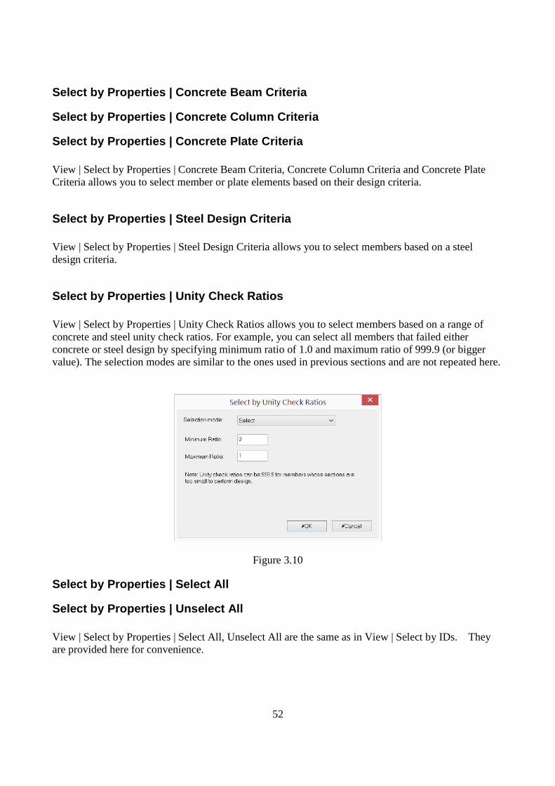
52

Select by Properties | Concrete Beam Criteria

Select by Properties | Concrete Column Criteria

Select by Properties | Concrete Plate Criteria View | Select by Properties | Concrete Beam Criteria, Concrete Column Criteria and Concrete Plate Criteria allows you to select member or plate elements based on their design criteria.

Select by Properties | Steel Design Criteria View | Select by Properties | Steel Design Criteria allows you to select members based on a steel design criteria.

Select by Properties | Unity Check Ratios View | Select by Properties | Unity Check Ratios allows you to select members based on a range of concrete and steel unity check ratios. For example, you can select all members that failed either concrete or steel design by specifying minimum ratio of 1.0 and maximum ratio of 999.9 (or bigger value). The selection modes are similar to the ones used in previous sections and are not repeated here.

Figure 3.10

Select by Properties | Select All

Select by Properties | Unselect All View | Select by Properties | Select All, Unselect All are the same as in View | Select by IDs. They are provided here for convenience.

53

Flip Selection View | Flip Selection flips the selection statuses of all entities in the entire model. The nodes and elements currently selected will be unselected and vice versa.

Freeze Selected View | Freeze Selected freezes or hides the selected nodes, elements and their dependents. The frozen nodes or elements are not displayed and are not modifiable unless the model integrity is at stake. This command allows you to focus on some particular parts of the model. For example, if you want to work on a particular floor of a three dimensional building, you may select the floor, flip the selection and freeze the selected elements.

Freeze All Except Selected View | Freeze All Except Selected freezes or hides all nodes and elements except the selected nodes, elements and their dependents.

Freeze All Except Level View | Freeze All Except Level freezes or hides the all nodes, elements and their dependents except those on the specified level (Figure 3.11). This command provides a shortcut to the previous command when you would like to focus on elements of the model in a horizontal plan view. You must have levels defined (through menu Geometry->Levels) before running this command.

Figure 3.11

Freeze All Except Plane View | Freeze All Except Plane freezes or hides the all nodes, elements and their dependents except those on the specified plane (Figure 3.12). This command provides a shortcut to the previous command when you would like to focus on elements of the model in a plan view.

54

Figure 3.12

Thaw View | Thaw allows you to thaw all frozen (hidden) nodes, elements and their dependents.

Load Diagram View | Load Diagram prompts you with the following dialog box (Figure 3.13). It allows you to view loads of selected types in selected load cases. You may have the options to show load magnitudes or units. The line load intervals may vary between 1 and 16. An interval between 2 to 6 is recommended. Transparency may be set for non-area loads and area loads so you can see objects underneath the loads. You can adjust plot scales between 1/10 ~ 10 for all loads based on the base scales set from Settings->Graphic Scales menu. You can preview the settings on this dialog box by clicking on Apply button. The displayed loads can be deleted by first select nodes and elements, then press the Delete key. The loads not displayed cannot be deleted unless their parent nodes or elements are deleted.

Figure 3.13

55

Annotate View | Annotate prompts you with the above dialog box (Figure 3.14). It allows you to view annotations for nodes and elements and their properties. The element local axes may also be displayed using this command. Three annotation modes are available. You may annotate all entities, annotate selected entities, and erase existing annotations. For performance reasons, it is recommended that the annotations be applied only for those objects which you are interested.

Figure 3.14

Query View | Query lets you query extensive input and output information for a single node, member or finite element (Figure 3.15). For example, a node query will list node id, nodal coordinates, nodal loads and additional nodal masses. It will also list relevant support or nodal spring information. If there are analysis results, it will list nodal displacements, support or spring reactions as well.

Distance View | Distance allows you to graphically pick two nodes and calculate the their distance. It also lists the angle in degrees in XY plane and the angle in degrees from XY plane. The result is displayed on the status bar.

56

Figure 3.15

Render | Render Options View | Render | Render Options prompts you with the following dialog box (Figure 3.16). It allows you to turn on or off the shading of the surfaces of members, shells and bricks as though they were illuminated from multiple light sources. It provides a way for you to realistically visualize the image of the model. For shells, you have the option to render thickness as well as surface. You have the option to apply different rendering percentages to different elements. Enter 100% for full rendering, 0% for no rendering, and anything in-between for partial rendering. The partial rendering (e.g. 50-80%) may be useful in identifying connectivity of elements to nodes.

Figure 3.16

57

Note: Rendering a model can be expensive in terms of memory and time usages by the program. You should turn off the rendering when it is not necessary.

Render | Quick Render View | Render | Quick Render turns rendering on or off. You may run this command by pressing F8.

Result Diagrams | Shear and Moment Diagram View | Result Diagrams | Shear and Moment Diagram prompts you with the following dialog box (Figure 3.17). It allows you to view the member shear (including axial force) diagram or moment (including torsion) diagram for the selected load combination. Only one shear or moment diagram for the selected load combination may be displayed per window. However, you may display different shear or moment diagrams in multiple windows. To open a new window, run Window | New Window. You have the option to show values and units for the diagram. You may show diagrams on all members or on selected members only. You may also erase existing diagrams. By default, no diagram is displayed even if an analysis has been performed successfully. You can adjust plot scales between 1/10 ~ 10 for shear and moment diagrams based on the base scales set from Settings->Graphic Scales menu. You can preview the settings on this dialog box by clicking on Apply button. You can adjust diagram scales using Settings | Graphics Scales menu. You can also fill the moment and shear diagrams by checking “Fill moment and shear diagrams” in Settings | Preferences menu.

Figure 3.17

Figure 3.18

Result Diagrams | Deflection Diagram

58

View | Result Diagrams | Deflection Diagram prompts you with the following dialog box (Figure 3.19). It allows you to view the deflected shape of the model for the selected load combination. The deflected shape is constructed by adding nodal displacements to nodal coordinates. For members, you have the option to show the local y and/or z deflection as well. You need to adjust the displacement magnification to view the deflection properly. The deflection displayed is for the selected load combination only. However, you may display deflections for different load combinations in multiple windows. To open a new window, run Window | New Window. The deflection values and units may be shown for the member local deflections. You may choose to have shadows of the un-deformed shape and deformed shape hidden. You cannot perform mouse selection while the deflected shape is shown. However, you may open another window with the un-deformed shape and perform mouse selection as usual.

Figure 3.19

Figure 3.20

Result Diagrams | Contour Diagram View | Result Diagrams | Contour Diagram prompts you with the following dialog box (Figure 3.21). It allows you to view a result contour for shells and/or bricks for the selected load combination. Four display modes are available. They are Iso-Surface and Value, Iso-Surface only, Value only, None or Erase. The Iso-Surface provides color bands for the contour component in different ranges. The number of ranges (or colors) may be either 16 or 8. Either top or bottom stresses may be specified for plate/shell elements. The Value (the absolute maximum) of the contour component may be shown for each element. The contour may be displayed in colors or gray scale. The latter is useful for people with color-impaired visions. The contour components include:

• nodal displacements (Dx, Dy, Dz, Dox, Doy, and Doz) • shell bending moments (Mxx, Myy, Mxy) and shears (Vxx, Vyy) • shell membrane normal forces (Fxx, Fyy) and in-plane shears (Fxy) • shell and brick stresses (Sxx, Syy, Szz, Sxy, Sxz, Syz) • surface spring reactions (SRx, SRy, SRz) • shell principal moments (Mmax, Mmin) and shear (Vmax)

59

• shell principal membrane forces (Fmax, Fmin) • principal stresses (S1, S2, S3) for shells and bricks • Von Mises stresses for shells and bricks

Figure 3.21 Only one contour component for the selected load combination may be displayed per window. However, you may display different contour components in multiple windows. To open a new window, run Window | New Window. Four different modulations may be applied to values of the contour component. They are “Positive and Negative”, “Absolute”, “Positive Only”, “Negative Only”. For example, you may choose the contour component “Mxx” and the modulation “Negative Only” to view only the negative moments Mxx of the plates. The following figure (Figure 3.22) shows a displacement (Dz) contour for a plate, with display mode “Iso-Surface and Values” and value modulation of “Positive and Negative”.

Figure 3.22

Result Diagrams | Mode Shape

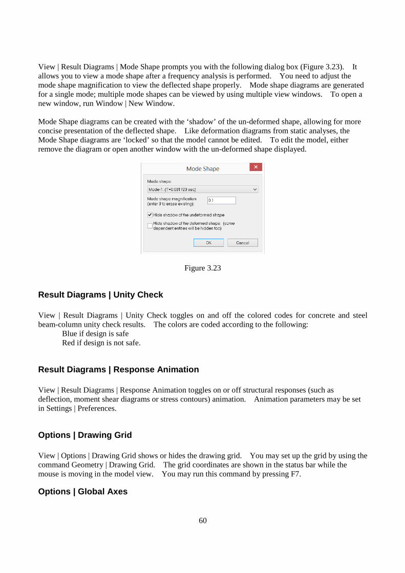
60

View | Result Diagrams | Mode Shape prompts you with the following dialog box (Figure 3.23). It allows you to view a mode shape after a frequency analysis is performed. You need to adjust the mode shape magnification to view the deflected shape properly. Mode shape diagrams are generated for a single mode; multiple mode shapes can be viewed by using multiple view windows. To open a new window, run Window | New Window. Mode Shape diagrams can be created with the ‘shadow’ of the un-deformed shape, allowing for more concise presentation of the deflected shape. Like deformation diagrams from static analyses, the Mode Shape diagrams are ‘locked’ so that the model cannot be edited. To edit the model, either remove the diagram or open another window with the un-deformed shape displayed.

Figure 3.23

Result Diagrams | Unity Check View | Result Diagrams | Unity Check toggles on and off the colored codes for concrete and steel beam-column unity check results. The colors are coded according to the following:

Blue if design is safe Red if design is not safe.

Result Diagrams | Response Animation View | Result Diagrams | Response Animation toggles on or off structural responses (such as deflection, moment shear diagrams or stress contours) animation. Animation parameters may be set in Settings | Preferences.

Options | Drawing Grid View | Options | Drawing Grid shows or hides the drawing grid. You may set up the grid by using the command Geometry | Drawing Grid. The grid coordinates are shown in the status bar while the mouse is moving in the model view. You may run this command by pressing F7.

Options | Global Axes

61

View | Options | Global Axes shows or hides the legend of the global axes in the bottom-left corner of the window. You may run this command by pressing F5.

Options | Contour Legend View | Options | Contour Legend shows or hides the contour legend. The results must exist for the contour legend to be displayed.

Options | Comment View | Options | Comment allows you to insert a comment at a specified location (Figure 3.24). The comment must be less than 256 characters in length. To remove an existing comment, go to Input Data | Comments spreadsheet and delete the comment entry.

Figure 3.24

62

Chapter 4: Geometry The Geometry menu provides commands to define and/or assign material, section, and thickness properties to selected elements; draw individual nodes and elements based on a drawing grid or existing nodes; parametrically generate models of regular shape; and define and/or assign boundary conditions or moment releases to selected elements or nodes.

Materials Geometry | Materials prompts you with the following dialog box (Figure 4.1). It allows you to define and/or assign materials to selected elements in the model. An Id is assigned automatically to each material by the program and may not be changed. You may assign a label with 127 maximum characters to each material for easy identification. The material properties include:

• Young’s modulus (E), • Poisson ratio (0 ≤ ν < 0.5). • Weight density. • Temperature coefficients.

The shear modulus (G) is calculated automatically, )1(2 ν+= E

G .

These material properties are used in the structural analysis of the model. Material properties related to design may be set from design menus. For example, concrete strength fc and reinforcement strengths fy and fys may be defined from RC Design | Design Criteria | RC Materials. You may add standard steel and concrete materials by clicking the “Std Materials” button. A standard material label starts with “Steel” or “Concrete”. You may add one or more materials by clicking the “New Rows” button. You may also print all materials in the list by clicking the “Print” button. The “Assign active material to currently selected elements” checkbox may be used to assign the active material to selected elements. The active material refers to the one that currently has focus in the list in the dialog box. In order for material assignments to take place, members, shells or bricks must be selected beforehand. A more flexible way to assign material and other properties to elements is to use Assign | Member Properties or Assign | Shell Properties command, which allows you to continuously assign one or more properties to elements. The program always has a default material labeled “Default”. You may not delete this material or change its label. You may, however, change its properties.

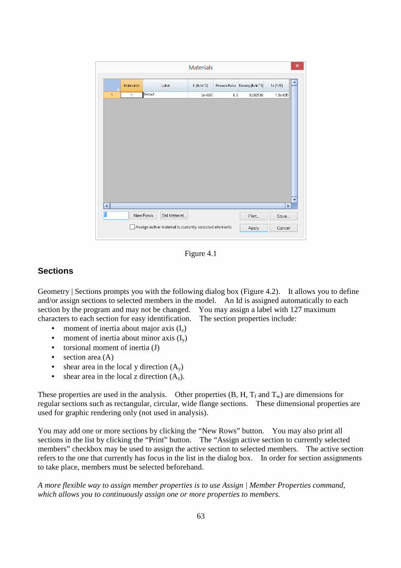
63

Figure 4.1

Sections Geometry | Sections prompts you with the following dialog box (Figure 4.2). It allows you to define and/or assign sections to selected members in the model. An Id is assigned automatically to each section by the program and may not be changed. You may assign a label with 127 maximum characters to each section for easy identification. The section properties include:

• moment of inertia about major axis (Iz) • moment of inertia about minor axis (Iy) • torsional moment of inertia (J) • section area (A) • shear area in the local y direction (Ay) • shear area in the local z direction (Az).

These properties are used in the analysis. Other properties (B, H, Tf and Tw) are dimensions for regular sections such as rectangular, circular, wide flange sections. These dimensional properties are used for graphic rendering only (not used in analysis). You may add one or more sections by clicking the “New Rows” button. You may also print all sections in the list by clicking the “Print” button. The “Assign active section to currently selected members” checkbox may be used to assign the active section to selected members. The active section refers to the one that currently has focus in the list in the dialog box. In order for section assignments to take place, members must be selected beforehand. A more flexible way to assign member properties is to use Assign | Member Properties command, which allows you to continuously assign one or more properties to members.

64

Note: The section property input does not include Ixy – the product of inertia. For a section where Ixy is not zero such as an angle, the principal axes of a cross section are different from its geometric axes. In such situations, you should enter section properties in its principal axes and adjust the member element local angle accordingly.

Figure 4.2 You may add a regular section by clicking the “Regular Section” button. The program displays the following dialog box (Figure 4.3). Three regular sections are currently provided by the program, namely rectangular, circular, wide flange and Tee sections. The properties of these sections are calculated automatically.

Figure 4.3

65

Figure 4.4 You may also add sections from the AISC steel shape table (Figure 4.4) or NDS wood shape table. You should not modify an AISC or NDS shape label or its properties. You may create one and only rigid link section for use in the model by simply click “Rigid Link” button. A rigid link is a member that has very large sectional properties (A, Ay, Az, Iz, Iy and J). There can only be one rigid link section defined in the model and it must be named as “RIGID_LINK”. The properties for the RIGID_LINK section must be set to 0’s on the member section dialog box. The program will appropriately calculate A, Ay, Az, Iz, Iy and J during the solution process. Self weight for rigid links will be ignored by the program. The program always has a default section labeled “Default”. You may not delete this section or change its label. You may, however, change its properties. AISC steel shapes can be customized by exporting and importing AISC tables. “Export AISC Table” will export AISC table database from this program to a csv (Comma Delimited) file. The exported csv file can then be modified in Microsoft Excel to add/remove/modify AISC steel shapes. “Import AISC Table” will import AISC Table to this program from a csv file. Importing AISC table will replace all AISC steel shape database contained in aisc14u.idx and aisc14u.tbl files in the program folder. As a precaution, you should backup these two files beforehand in case something goes wrong during importing. The csv file to be imported must conform to the format that the program exports. You may use dot(.) in AISC_Manual_Label column to distinguish new shapes with existing shapes. For example, W16.99X89.99 is a valid shape name.

Thicknesses Geometry | Thicknesses prompts you with the following dialog box (Figure 4.5). It allows you to define and/or assign thicknesses to selected shells in the model. An Id is assigned automatically to each thickness by the program and may not be changed. You may assign a label with 127 maximum characters to each thickness for easy identification. The thickness properties include thickness only.

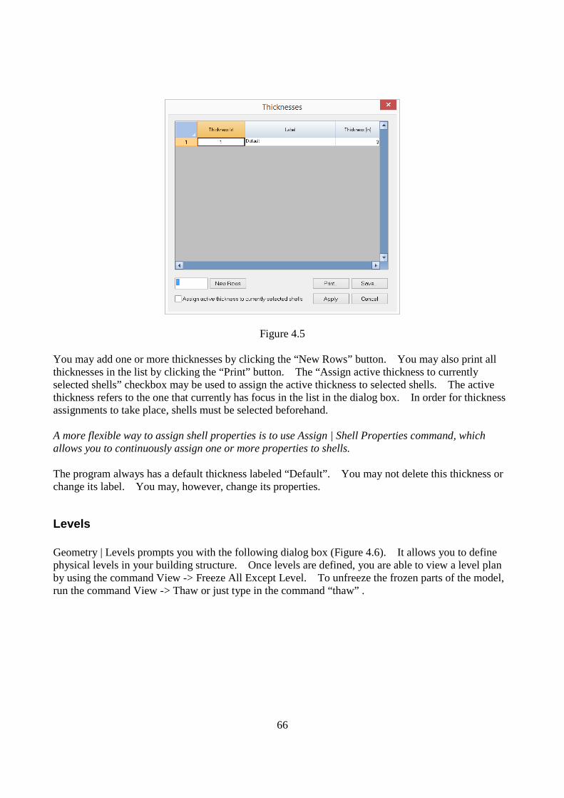
66

Figure 4.5 You may add one or more thicknesses by clicking the “New Rows” button. You may also print all thicknesses in the list by clicking the “Print” button. The “Assign active thickness to currently selected shells” checkbox may be used to assign the active thickness to selected shells. The active thickness refers to the one that currently has focus in the list in the dialog box. In order for thickness assignments to take place, shells must be selected beforehand. A more flexible way to assign shell properties is to use Assign | Shell Properties command, which allows you to continuously assign one or more properties to shells. The program always has a default thickness labeled “Default”. You may not delete this thickness or change its label. You may, however, change its properties.

Levels Geometry | Levels prompts you with the following dialog box (Figure 4.6). It allows you to define physical levels in your building structure. Once levels are defined, you are able to view a level plan by using the command View -> Freeze All Except Level. To unfreeze the frozen parts of the model, run the command View -> Thaw or just type in the command “thaw” .

67

Figure 4.6

Drawing Grid Geometry | Drawing Grid prompts you with the following dialog box (Figure 4.7). It allows you to generate a 1D, 2D or 3D rectangular grid for drawing or guidance. The distance list is a comma separated list that specifies multiple distances. For example, a distance list of “12, 2@14, 3@10” will generate distances of 12, 14, 14, 10, 10 and 10 in length units. You may specify a distance list for the X, Y, or Z direction or any combination of them. You may specify an insertion point to translate and rotation parameters to rotate the grid. The drawing grid may be turned on or off by running the command View | Drawing Grid or by simply pressing F7. You may regard the grid as a user defined coordinate system that can be changed at any time. The coordinates of the grid intersection under the mouse are displayed in the status bar. It helps you to identify correct points when drawing nodes or elements. The following example (Figure 4.8) shows the use of this command.

Figure 4.7

Figure 4.8

68

Object Snap The Geometry | Object Snap pop-up menu provides options to snap node locations at 1/2, 1/3, … 1/9th points on a member under the mouse cursor. If you are drawing elements, you also have the option to snap to the perpendicular point on a member from the last point. It is a good idea to turn off the drawing grid (by pressing F7) to avoid snapping to grid points while any of the snap options is on.

Draw Node Geometry | Draw Node allows you to draw new nodes in the model. To draw a node, simply move the mouse, point to an intersection of the grid and click the left mouse button. You may also draw a node by entering nodal X, Y, and Z (optional) coordinates in the command window via the keyboard. This is very useful if you need to draw nodes outside the grid interactions. The command remains in effect until another command is selected, the right mouse button is clicked, or ESC is pressed.

Draw Member Geometry | Draw Member allows you to draw new members in the model. To draw a member, simply move the mouse and click the left mouse button from point to point (Figure 4.9). The clicked points must be intersections on the grid or existing nodes. These points become the element nodes. New nodes are created if necessary. Members are drawn continuously. Right clicking the mouse once lets you start drawing members from a new location. Remember, the start and end nodes determine the default local coordinate system. The members drawn have the current section and material properties. You may use the commands in the Geometry menu to assign appropriate properties to them. You may also specify a node by entering nodal X, Y and Z (optional) coordinates in the command window via the keyboard. This is very useful if you need to specify nodes outside the grid interactions. In addition, you may specify a node by entering an existing node number directly. You can combine the use of keyboard and mouse to draw members. You may turn on annotations for nodes and members while drawing. To do that, run View | Annotate. The command remains in effect until another command is selected, the right mouse button is clicked twice, or ESC is pressed.

69

Figure 4.9

Figure 4.10

Draw Shell4 Geometry | Draw Shell4 allows you to draw new shells in the model. To draw a shell, simply move the mouse and click the left mouse button from point to point (Figure 4.10). The clicked points must be intersections on the grid or existing nodes. These points become the element nodes. New nodes are created if necessary. Remember, the order of clicked points determines the default local coordinate system. The shells drawn have the current thickness and material properties. You may use the commands in the Geometry menu to assign appropriate properties to them. You may also specify a node by entering nodal X, Y, and Z (optional) coordinates in the command window via the keyboard. This is very useful if you need to specify nodes outside the grid interactions. In addition, you may specify a node by entering an existing node number directly. You can combine the use of keyboard and mouse to draw shell4s. You may turn on annotations for nodes and shells while drawing. To do that, run View | Annotate. The command remains in effect until another command is selected, the right mouse button is clicked, or ESC is pressed.

Draw Brick Geometry | Draw Brick allows you to draw new bricks in the model. To draw a brick, simply move the mouse and click the left mouse button from point to point (Figure 4.11). The grid must be set up in 3 dimensions. The clicked points must be intersections on the grid or existing nodes. These points become the element nodes. New nodes are created if necessary. Remember, the order of clicked points must be such that the vector of the surface 1-2-3-4 points to the surface 5-6-7-8. The bricks drawn have the current material properties. You may use the commands in the Geometry menu to assign appropriate properties to them.

70

You may also specify a node by entering nodal X, Y, and Z coordinates in the command window via the keyboard. This is very useful if you need to specify nodes outside the grid interactions. In addition, you may specify a node by entering an existing node number directly. You can combine the use of keyboard and mouse to draw bricks. You may turn on annotations for nodes and bricks while drawing. To do that, run View | Annotate. The command remains in effect until another command is selected, the right mouse button is clicked, or ESC is pressed.

Figure 4.11 It is generally not easy to draw bricks in 3 dimensions due to visualization difficulty. You may generate bricks based on shells using the commands such as Edit | Extrude or Revolve. You may also use spreadsheets to input nodes and bricks by running Input Data | Nodes or Bricks.

Quick Draw | Member Geometry | Quick Draw | Member allows you to draw a member by specifying the two element nodes in the command window.

Quick Draw | Shell4

Quick Draw | Brick Geometry | Quick Draw | Shell4 or Brick command is similar to Member command above.

Generate The Geometry | Generate pop-up menu provides commands to quickly generate commonly used structural components in a model. These commands may be run multiple times to generate different parts in the model. You may use edit commands such as Edit | Duplicate, Move, Delete, etc. to modify the generated model.

71

Generate | Rectangular Frames Geometry | Generate | Rectangular Frames prompts you with the following dialog box (Figure 4.12). It allows you to quickly generate 1D frames (continuous beams), 2D frames (plane frame or grillage) or 3D frames (space frames). The distance list is a comma separated list that specifies multiple distances. For example, a distance list of “12, 2@14, 3@10” will generate distances of 12, 14, 14, 10, 10 and 10 in length unit. You may leave appropriate distance list(s) blank to generate on a plane or along a line. You may specify pinned or fixed supports at the bottom. The generated members have the default section and material properties. You may assign them appropriate properties using commands in the Geometry menu.

Figure 4.12 The following three examples show the uses of this command. The first example (Figure 4.13) is a continuous beam in the X direction generated using the input from the dialog box above. The first two spans are of 10 ft and the last three spans are of 15 ft. The pinned supports are also generated automatically.

Figure 4.13

The second example (Figure 4.14) is a 2D frame on the XY plane with horizontal spans 10, 10, 18, 10, 10 ft and vertical spans 15, 8, 8, 8 ft as shown in the following. A rectangular frame is first generated using the input from the following dialog box (Figure 4.15). The frame is then modified by selecting and deleting nodes 19, 24, 25, 26, 29, 30 and horizontal members at the bottom (Figure 4.16). Notice when a node is deleted, elements (and their dependents such as loads) connected to that node are automatically deleted also.

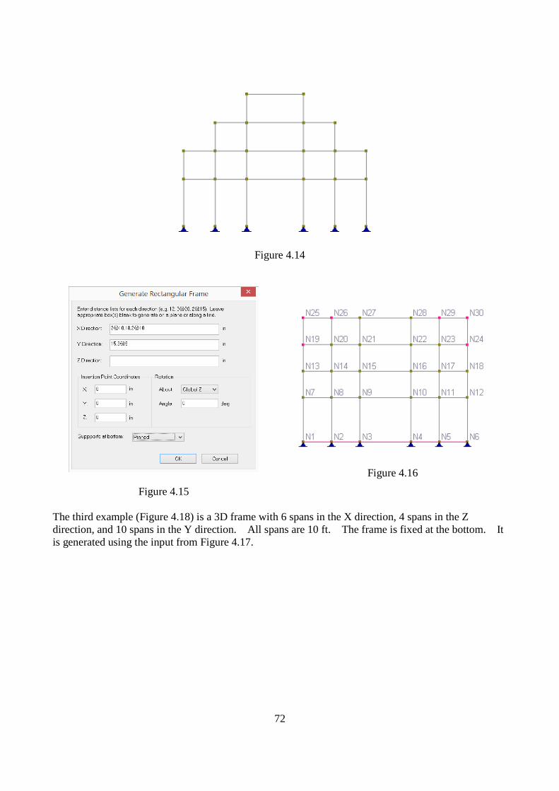
72

Figure 4.14

Figure 4.15

Figure 4.16

The third example (Figure 4.18) is a 3D frame with 6 spans in the X direction, 4 spans in the Z direction, and 10 spans in the Y direction. All spans are 10 ft. The frame is fixed at the bottom. It is generated using the input from Figure 4.17.

73

Figure 4.17

Figure 4.18

Generate | Cylindrical Frames Geometry | Generate | Cylindrical Frames prompts you with the following dialog box (Figure 4.19). It allows you to quickly generate 2D or 3D cylindrical frames. The distance list is a comma separated list that specifies multiple distances. For example, a distance list of “12, 2@14, 3@10” will generate distances of 12, 14, 14, 10, 10 and 10 in length unit. You may leave the Y direction distance list empty, in which case, a plane cylindrical frame will be generated. You may specify pinned or fixed supports at the bottom. The generated members have the default section and material properties. You may assign them appropriate properties using commands in the Geometry menu. You have the option not to generate members. In this way, you can generate nodes on cylindrical system first. Then you may use the command Generate | Shells (Bricks) by Nodes to generate a system of shell (brick) elements.

Using the input in Figure 4.19, a 3D cylindrical frame in Figure 4.20 is generated. You may need to set the element local angles for columns for correct orientation.

74

Figure 4.19

Figure 4.20

Generate | Rectangular Shell4s Geometry | Generate | Rectangular Shell4s prompts you with the following dialog box (Figure 4.21). It allows you to quickly generate shells in a rectangle. The distance list is a comma separated list that specifies multiple distances. For example, a distance list of “12,2@14,3@10” will generate distances of 12, 14, 14, 10, 10 and 10 in length units. You may specify an insertion point to translate and rotation parameters to rotate the generated shells. The generated shells have the default thickness and material properties. You may assign them appropriate properties using commands in the Geometry menu.

Figure 4.21

Figure 4.22

75

This command can only generate shells in a rectangle. To generate shells in a general quadrilateral, you may first define one quadrilateral shell and then use the command Edit | Sub-Mesh Shell4s to sub-divide it. The above example (Figure 4.22) shows a 10x10 rectangular mesh of shells generated using the input from Figure 4.21.

Generate | Circular Shell4s Geometry | Generate | Circular Shell4s prompts you with the following dialog box (Figure 4.23). It allows you to quickly generate shells in a circle. You may specify the number of segments to control the fineness of the mesh. Generally speaking, a relatively fine mesh is recommended to minimize the discretization error along the curved edge. The generated shells are mostly rectangular in shape, with some general quadrilaterals along the edge. You should not use rectangular thin plate formulation in the analysis. You may specify an insertion point to translate and rotation parameters to rotate the generated shells. The generated shells have the default thickness and material properties. You may assign them appropriate properties using commands in the Geometry menu. The following example (Figure 4.24) shows shells generated in a circle using the input from Figure 4.23.

Figure 4.23

Figure 4.24

Generate | Arc Members Geometry | Generate | Arc Members prompts you with the following dialog box (Figure 4.25). It allows you to quickly generate members along an arc. You may specify an arc radius, the start and end angles, and the number of segments. You may specify an insertion point to translate and rotation parameters to rotate the generate shells. The generated members have the default section and material properties. You may assign them appropriate properties using commands in the Geometry menu.

76

The following example (Figure 4.26) shows members generated along an arc using the input from Figure 4.25.

Figure 4.25

Figure 4.26

Generate | Non-Prismatic Members Geometry | Generate | Non-Prismatic Members prompts you with the following dialog box (Figure 4.27). It allows you to quickly convert each of the selected prismatic members into multiple prismatic members to approximate a non-prismatic member. The distance list is a comma separated list that specifies multiple distances. For example, a distance list of “12, 2@14, 3@10” will generate distances of 12, 14, 14, 10, 10 and 10 in length units. The lengths of the selected prismatic members must be consistent with the distance list.

Figure 4.27

The left and right haunches of the non-prismatic members may be of type linear, parabolic or straight. You must define the geometry (Figure 4.28) including middle depth (DM), left depth (DL), right depth (DR), width, left length ratio (LL / L), right length ratio (LR / L). Each of the selected prismatic members will be exploded into multiple prismatic members to approximate the non-prismatic member’s behavior. Appropriate member sections will be automatically added and assigned in the

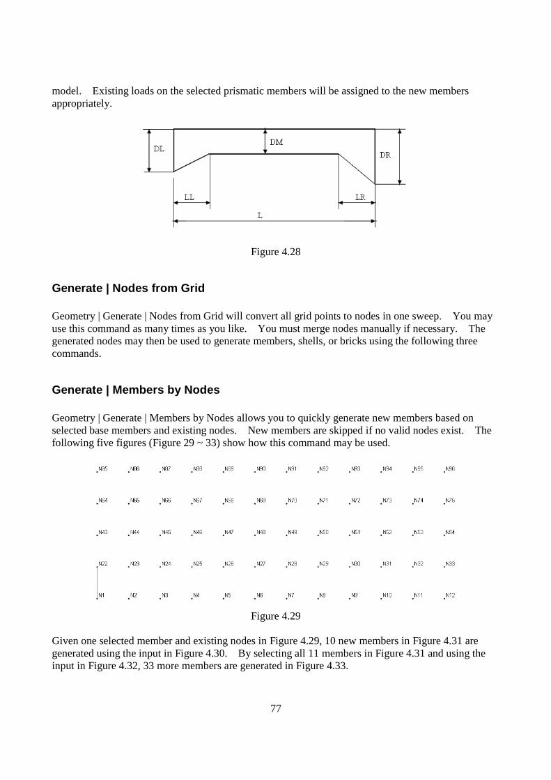
77

model. Existing loads on the selected prismatic members will be assigned to the new members appropriately.

Figure 4.28

Generate | Nodes from Grid Geometry | Generate | Nodes from Grid will convert all grid points to nodes in one sweep. You may use this command as many times as you like. You must merge nodes manually if necessary. The generated nodes may then be used to generate members, shells, or bricks using the following three commands.

Generate | Members by Nodes Geometry | Generate | Members by Nodes allows you to quickly generate new members based on selected base members and existing nodes. New members are skipped if no valid nodes exist. The following five figures (Figure 29 ~ 33) show how this command may be used.

Figure 4.29

Given one selected member and existing nodes in Figure 4.29, 10 new members in Figure 4.31 are generated using the input in Figure 4.30. By selecting all 11 members in Figure 4.31 and using the input in Figure 4.32, 33 more members are generated in Figure 4.33.

78

Figure 4.30

Figure 4.31

Figure 4.32

79

Figure 4.33

Generate | Shells by Nodes Geometry | Generate | Shells by Nodes allows you to quickly generate new shells based on selected base shells and existing nodes. New shells are skipped if no valid nodes exist. The concept in this command is similar to Generate | Members by Nodes.

Generate | Bricks by Nodes Geometry | Generate | Bricks by Nodes allows you to quickly generate new bricks based on selected base bricks and existing nodes. New bricks are skipped if no valid nodes exist. The concept in this command is similar to Generate | Members by Nodes.

Element Local Angle Geometry | Element Local Angle prompts you with the above dialog box (Figure 4.34). It allows you to assign local angles to the selected members and/or shells. The element local angle is used to change the element local coordinate system.

Figure 4.34

3-Point Member Orientation

80

Geometry | 3-Point Member Orientation is the same as Edit | 3-Point Member Orientation. This command is listed here for convenience only.

Moment Releases Geometry | Moment Releases prompts you with the following dialog box (Figure 4.35). It allows you to assign moment releases to selected members in the model. Major, minor moment releases may be applied to the start and/or end ends of the members. Torsional moment may be applied to either the start or end end (but not both ends) of the members. Trusses are members with major and minor moments fully released at both ends, and torsional moment released at either end of the members. The program assigns appropriate moment releases automatically if the model type is of “2D Truss” or “3D Truss”. However, if the model contains both trusses and beams, you should use the model type “2D Frame” or “3D Frame”, and assign appropriate moment releases to members. A truss member is a beam with major and minor moment releases at both ends, as well as torsional moment release at either one end (but not both ends) of the member. In order for moment release assignments to take place, members must be selected beforehand.

Figure 4.35

Rigid Offset Geometry | Rigid Offset prompts you with the above dialog box (Figure 4.36). It allows you to assign rigid offsets to the selected members. This command will effectively break each selected member into two or three members, with either or both ends being rigid links.

81

Figure 4.36

Tension/Compression Only Geometry | Tension/Compression Only prompts you with the above dialog box (Figure 4.37). It allows you to assign nonlinearity (linear, tension only or compression only) to the selected members. The member stiffness will be ignored if a tension only member is subjected to compressive forces or if a compression only member is subjected to tensile forces. The presence of tension only or compression only members makes the model nonlinear and requires iterative solution for each load combination.

Figure 4.37

Convert Members to Rigid Links Geometry | Convert Members to Rigid Links will convert selected members to rigid links. This is the same command as Edit | Convert Members to Rigid Links.

Element Activation Geometry | Element Activation is identical to Edit | Element Activation.

Supports

82

Geometry | Supports prompts you with the following dialog box (Figure 4.38). It allows you to assign supports (rigid boundary conditions) to selected nodes in the model. One or more of the six global degrees of freedom (DOFs) may be restrained. In addition, you may specify enforced displacements in the restrained DOFs. The enforced displacements may be used to model support settlements. You may regard them as special loads. For normal supports, enforced displacements in the restrained DOFs are zero. The program provides three commonly used supports, namely, pinned, fixed and roller (Figure 4.39). In order for support assignments to take place, nodes must be selected beforehand.

Figure 4.38

Figure 4.39

A more flexible way to assign supports is to use Assign | Support command, which allows you to continuously assign one or more support to nodes.

Springs Geometry | Springs prompts you with the following dialog box (Figure 4.40). It allows you to assign nodal, line, and surface springs (flexible boundary conditions) to selected nodes, members, or shells in the model (Figure 4.41). A nodal spring may be restrained in one or more of the six global DOFs (Dx, Dy, Dz, Dox, Doy and Doz). A line or surface spring may be restrained in one or more of the three global translational DOFs (Dx, Dy and Dz). To qualify to be a valid flexible restraint, the corresponding spring constant must be specified.

83

Figure 4.40

Figure 4.41

A restraint may be designated as linear, compression-only or tension only. A compression-only restraint is active only when the nodal displacement in the restrained direction is negative. A tension-only restraint is active only when the nodal displacement in the restrained direction is positive. The presence of tension only or compression only springs makes the model nonlinear and requires iterative solution for each load combination. A more flexible way to assign springs is to use Assign | Spring command, which allows you to continuously assign one or more springs to nodes, members or shells.

Coupled Springs Geometry | Coupled Springs prompts you with the following dialog box (Figure 4.41a). It allows you to assign coupled springs to selected nodes. Coupled springs are useful in modeling/simplifying sub-structures such as bridge foundations. It is important to enter the coupled spring stiffness matrix in the appropriate units.

Figure 4.41a

84

Diaphragms Geometry | Diaphragms prompts you with the following dialog box (Figure 4.42). It allows you to define regular or generic rigid diaphragms (in-plane) in a 3D model. For example, to model horizontal concrete floors, you may select one node on each floor and apply regular diaphragms to the selected nodes in XZ plane (with normal in the global Y direction). Instead of using plate elements, rigid diaphragms allow you to model stiff in-plane actions quickly. The program further provides the option to ignore the rigid diaphragm actions as an analysis option (Run | Analysis Options).

Figure 4.42

Multi-DOF Constraints | Inclined Rollers Geometry | Multi-DOF Constraints | Inclined Rollers prompts you with the following dialog box (Figure 4.43). It allows you to define an inclined roller support on XY, YZ or XZ plane. An inclined roller can only move along the line between the reference point (defined in the dialog) and the support location. For example in Figure 4.44, the roller is located at coordinate (8.0, 5.0, 0) and is inclined 30 degrees from the X-axis. We can use the reference point (8.0 + 10 * cos30, 5 + 10 * sin30, 0) = (16.666, 10, 0) to constrain the support. An inclined roller is a type of multi-DOF constraint. A regular support and multi-DOF constraints may be applied on the same node as long as the support/constrained directions do not interfere with each other. Multi-DOF constraint forces and moments are listed separately from the regular support reactions in the analysis results.

85

Figure 4.43

Figure 4.44

Multi-DOF Constraints | Equal Displacement Constraints Geometry | Multi-DOF Constraints | Equal Displacement Constraints prompts you with the following dialog box (Figure 4.45). It allows you to define a generic constraint at one or two nodes. An equal displacement constraint is one type of multi-DOF constraint. A regular support and multi-DOF constraints may be applied on the same node as long as the support/constrained directions do not interfere with each other. Multi-DOF constraint forces and moments are listed separately from the regular support reactions in the analysis results.

86

Figure 4.45

Multi-DOF Constraints | Generic Constraints Geometry | Multi-DOF Constraints | Generic Constraints prompts you with the following dialog box (Figure 4.46). It allows you to define a generic constraint at one or two nodes. If the constraint is applied to the same node, the constraint DOFs must be different. Constrained DOFs must be compatible: Q1 and Q2 must be both translational or rotational. Constraint factors must be non-zero. A regular support and multi-DOF constraints may be applied on the same node as long as the support/constrained directions do not interfere with each other. Multi-DOF constraint forces and moments are listed separately from the regular support reactions in the analysis results.

Figure 4.46

Story Drift Nodes Geometry | Story Drift Nodes allows you to assign selected nodes as nodes for floor drift calculation. All story drift nodes can be viewed in Input Data | Story Drift Nodes spreadsheet. The story drift results can be viewed from the Analysis Results | Story Drifts menu.

87

Chapter 5: Loads The Loads menu provides commands to define load cases and combinations, and assign loads of various types to selected nodes and elements.

Load Cases Loads | Load Cases prompts you with the following dialog box (Figure 5.1). It allows you to define load cases to be used for loads and load combinations. A number is assigned to each load case automatically by the program. You may assign a label with 127 maximum characters to each load case for easy identification. Duplicate labels in load cases are not allowed. A load type specifies the characteristics of the load case. Examples are DEAD, LIVE, WIND, EARTHQUAKE. They are used to generate standard load combinations in Loads | Load Combinations.

Figure 5.1 You may add one or more load cases by clicking the “New Rows” button. You may also print all load cases in the list by clicking the “Print” button. The program always has a default load case labeled “Default”. You may not delete this load case or change its label. You may however change its type.

Load Combinations

88

Loads | Load Combinations prompts you with the following dialog box (Figure 5.2). It allows you to define combinations of existing load cases in the model. The program solves for load combinations but not for load cases. You may assign a label with 127 maximum characters to each load combination for easy identification. Duplicate labels in load combinations are not allowed. You may add one load combination by clicking the “Add” button. You may then define the new load combination in the following dialog box (Figure 5.3). The definition includes a label with 127 maximum characters, a load factor for each load case, and a P-Delta flag. A load factor of zero excludes the respective load case from participating in the load combination. You may print all load cases and their corresponding load factors in the list by clicking the “Print” button. You may enter response spectrum load factor if you intend to combine response spectrum modal combination results with static analysis results for the load combination. The response spectrum analysis must be performed if any of load combinations contains a non-zero response spectrum load factor. No separate static analysis is needed. If you need to design concrete beams, columns and/or plates, check or uncheck “Perform Concrete Design using this Load Combination”. In addition, a sustained load factor must also be entered. This is the load factor that applies to the sustained load cases included in this load combination. It is

used to compute the infamousdβ during concrete column design. Therefore, if there are concrete columns to be designed, you should define a separate load combination that contains only sustained load cases (each case with a unit factor). You can then designate this load combination as the sustained load combination by RC Design | Design Options before performing concrete design. If you need to design steel members, check or uncheck “Perform Steel Design using this Load Combination”. If you need to use the load combination to check total or live load deflection, check or uncheck appropriate boxes. You may modify, copy, or delete a load combination by clicking the “Modify”, “Copy”, or “Delete” button. You may also create a load combination for every load case with a unit load factor for the load case but zeros for the rest of the load cases. To do that, click the “Unit Cases” button. You may also generate standard load combinations based on design codes such as ACI 318-02/05/08/11/14 by clicking the button “Generate Std”. There must be at least one load combination in a model.

89

Figure 5.2

Figure 5.3

Nodal Loads Loads | Nodal Loads prompts you with the following dialog box (Figure 5.4). It allows you to assign nodal loads to selected nodes in the model. You must select a load case to which the nodal loads belong. Nodal loads are specified in the global coordinate system. The loads are nodal forces in the X, Y, or Z direction if radio button “X”, “Y”, or “Z” is selected. The loads are nodal moments in the

90

X, Y, or Z direction if radio button “OX”, “OY”, or “OZ” is selected. The load magnitude may be any non-zero value.

Figure 5.4 A more flexible way to assign nodal load is to use Assign | Nodal Load command, which allows you to continuously assign one or more nodal loads to nodes.

Point Loads Loads | Point Loads prompts you with the above dialog box (Figure 5.5). It allows you to assign point loads to selected members in the model. You must select a load case to which the point loads belong. Point loads may be specified in either the local or global coordinate system. The loads are point forces in the X, Y, or Z direction if radio button “X”, “Y”, or “Z” is selected. The loads are point moments in the X, Y, or Z direction if radio button “OX”, “OY”, or “OZ” is selected. The load magnitude may be any non-zero value. The load distance is the ratio of the load location (measured from the member start) to the member length. A distance of 0.5 places the load at the middle of each selected member.

Figure 5.5 A more flexible way to assign point load is to use Assign | Point Load command, which allows you to continuously assign one or more point loads to members.

91

Line Loads Loads | Line Loads prompts you with the following dialog box (Figure 5.6). It allows you to assign line loads to selected members in the model. You must select a load case to which the line loads belong. Line loads may be specified in either the local or global coordinate system. The loads are line forces in the X, Y, or Z direction. The start and end magnitudes of the load may be zero for either end but not for both. The load distances are the ratios of the load start and end locations (measured from the member start) to the member length. A start distance of 0.0 and an end distance of 1.0 place the line load on the entire span of each selected member.

Figure 5.6 A more flexible way to assign line load is to use Assign | Line Load command, which allows you to continuously assign one or more line loads to members.

Area Loads Loads | Area Loads prompts you with the following dialog box (Figure 5.7). It allows you to assign area loads to enclosed areas of members in the model. You must select a load case to which the area loads belong. Area loads may be specified in either the local or global coordinate system. Global area loads may be in the global X, Y, or Z direction. Local area loads may only be in the local z direction, which is perpendicular to the load area. A load area is defined by specifying three or four coplanar nodes. The area load is then distributed as line loads to perimeter members of enclosed areas within the load area prior to static or dynamic solution. Various area load distribution methods are available. It is recommended that area loads be defined in their own load cases. In this way, you will find it easier to identify, edit, and delete area loads later on. The program also allows you to convert area loads to line loads automatically. This feature lets you see how the program would convert the area loads prior to the solution. For more information on the load conversion, see Input Data | Area Loads.

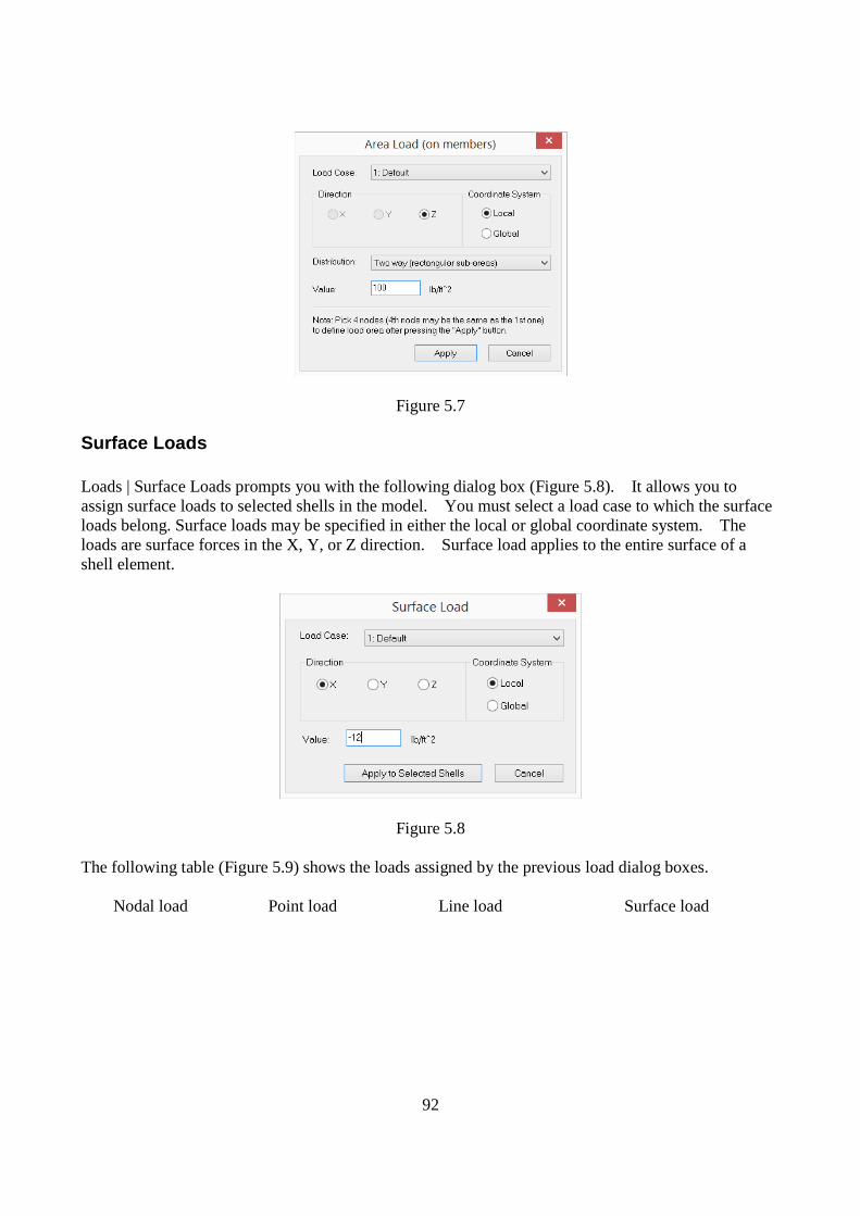
92

Figure 5.7

Surface Loads Loads | Surface Loads prompts you with the following dialog box (Figure 5.8). It allows you to assign surface loads to selected shells in the model. You must select a load case to which the surface loads belong. Surface loads may be specified in either the local or global coordinate system. The loads are surface forces in the X, Y, or Z direction. Surface load applies to the entire surface of a shell element.

Figure 5.8 The following table (Figure 5.9) shows the loads assigned by the previous load dialog boxes.

Nodal load Point load Line load Surface load

93

Figure 5.9

A more flexible way to assign surface load is to use Assign | Surface Load command, which allows you to continuously assign one or more surface loads to shells.

Thermal Loads Loads | Thermal Loads prompts you with the following dialog box (Figure 5.10). It allows you to assign thermal loads to selected elements in the model. You must select a load case to which the surface loads belong. Currently, Real3D considers thermal effect in longitudinal direction of members, membrane directions of shells, and bricks. It does not consider thermal gradients in members or shells.

Figure 5.10

Self Weights Loads | Self Weights prompts you with the following dialog box (Figure 5.11). It allows you to define how the program computes self weights for elements in the model that are not excluded in self weight (see Edit | Self Weight Exclusion). You must select a load case to which self weights belong. The self weights may act in the global X, Y, or Z direction. By default, self weights act in the global Y direction. You may specify a self weight multiplier (applied to material densities). A zero multiplier ignore self weights altogether.

94

Figure 5.11

Self Weight Exclusion Loads | Self Weight Exclusion is identical to Edit | Self Weight Exclusion.

Generate Loads | Fluid Loads Loads | Generate Loads | Fluid Loads prompts you with the dialog box above (Figure 5.12). It allows you to generate fluid loads applied to selected shells in the model. You must select a load case to which the fluid loads belong. Fluid loads are applied in the local coordinate system. The load variation must be in global X, Y or Z direction.

Figure 5.12

Generate Loads | Pattern Loads Loads | Generate Loads | Pattern Loads prompts you with the following dialog box (Figure 5.13). It allows you to generate pattern loads applied to specified members in the model. You must select a load case (generally live case) that contains loads to be patterned. A pattern ratio (e.g., ACI 318-05 specifies 0.75) is also available. Load patterning allows us to generate maximum positive and negative

95

moment at each span, maximum positive and negative moment at each support as well as maximum shear at each support. The existing point and line loads in the load case will be patterned based on odd, even and adjacent/alternate spans. These patterned loads are assigned to their own load cases. The program automatically generates additional load cases and load combinations based on the load patterning.

Figure 5.13 It should be pointed out that the program does not consider support conditions for pattern load generation. One pattern load case cannot be used in more than one load combination prior to load pattern generation.

Generate Loads | Moving Loads Loads | Generate Loads | Moving Loads prompts you with the dialog box above (Figure 5.14). It allows you to generate moving loads applied to specified members in the model. You must select a load case that contains moving loads. Only point loads on the specified members in the load case will be moved. These moving loads are assigned to their own load cases. The program automatically generates additional load cases and load combinations based on the moving step size. It should be pointed out that one moving load case cannot be used in more than one load combination prior to moving load generation.

96

Figure 5.14

Case-Copy Loads Loads | Case-Copy Loads prompts you with the following dialog box (Figure 5.15). It allows you to copy all loads from one load case to another. You have the option to delete existing loads in the target load case. The loads copied may also be multiplied by a factor. At least two load cases must exist in the model in order to run this command.

Figure 5.15

Convert Area Loads to Line Loads Loads | Convert Area Loads to Line Loads will convert all area loads to line loads in every load case. This is useful in checking how area loads would be converted during the solution process. You can always undo the area loads to line loads conversion.

97

Convert Local Loads to Global Loads Loads | Convert Local Loads to Global Loads will convert all member point loads, line loads and shell surface loads from local coordinate systems to global coordinate system in every load case. This is useful for data transfer from Real3D to Revit Structure using Real3D Revit Link. You can always undo the local loads to global loads conversion.

Additional Masses Loads | Additional Masses prompts you with the dialog box below (Figure 5.16). It allows you to assign additional masses and mass moment of inertia to selected nodes. The mass can be applied to X, Y and/or Z directions while the mass moment of inertia can be applied to OX, OY and/or OZ directions. Additional Masses are added to the mass calculated from the load combination for frequency analysis (see the command: Run | Frequency Analysis). Mass moment of inertia values can only be input using the Additional Masses command. The mass unit is a force unit divided by the acceleration of gravity, while the mass moment of inertia has units of mass times length squared. The acceleration of gravity is taken as 386.09 in/sec^2 or 9.8 m/sec^2.

Figure 5.16

A more flexible way to assign additional masses is to use Assign | Additional Masses command, which allows you to continuously assign additional masses to nodes.

Response Spectra Library Loads | Response Spectra Library prompts you with the dialog box below (Figure 5.17). It allows you to define spectrums for current and future projects. You can then use one or more spectrums in Run | Response Spectrum Analysis. You may view/modify a user-defined spectrum by double clicking the spectrum (Figure 5.18). The first spectrum can not be edited or deleted. Spectrums generated based on building codes cannot be edited but can be deleted.

98

Figure 5.17

Figure 5.18

99

Chapter 5A: Assign The Assign menu provides commands to continuously assign supports, springs, element properties and loads to relevant objects (nodes and elements). Unlike commands in other menus, you do NOT need to select objects before running these commands.

Supports The Assign | Supports prompts you with the following dialog (Figure 5A.1). The input is essentially the same as Geometry | Supports. After clicking “Assign”, you can start to continuously assign supports by window-selecting nodes until you right click the mouse or press the ESC key.

Figure 5A.1

Springs The Assign | Springs prompts you with the following dialog (Figure 5A.2). The input is essentially the same as Geometry | Springs. After clicking “Assign”, you can start to continuously assign nodal, line or surface springs by window-selecting nodes, members or shells until you right click the mouse or press the ESC key.

Member Properties The Assign | Member Properties prompts you with the following dialog (Figure 5A.3). It allows you to assign one or more properties such as material, section etc. to members. Make sure the “Use” checkbox by each property is set correctly. After clicking “Assign”, you can start to continuously assign all checked properties by window-selecting members until you right click the mouse or press the ESC key.

100

Figure 5A.2

Figure 5A.3

101

Shell Properties The Assign | Shell Properties prompts you with the following dialog (Figure 5A.4). It allows you to assign one or more properties such as material, thickness etc. to shells. Make sure the “Use” checkbox by each property is set correctly. After clicking “Assign”, you can start to continuously assign all checked properties by window-selecting shells until you right click the mouse or press the ESC key.

Figure 5A.4

Nodal Loads The Assign | Nodal Loads prompts you with the following dialog (Figure 5A.5). The input is essentially the same as Load | Nodal Loads. After clicking “Assign”, you can start to continuously assign nodal loads by window-selecting nodes until you right click the mouse or press the ESC key.

Figure 5A.5

Point Loads

102

The Assign | Point Loads prompts you with the following dialog (Figure 5A.6). The input is essentially the same as Load | Point Loads. After clicking “Assign”, you can start to continuously assign point loads by window-selecting members until you right click the mouse or press the ESC key.

Figure 5A.6

Line Loads The Assign | Line Loads prompts you with the following dialog (Figure 5A.7). The input is essentially the same as Load | Line Loads. After clicking “Assign”, you can start to continuously assign line loads by window-selecting members until you right click the mouse or press the ESC key.

Figure 5A.7

Surface Loads

103

The Assign | Surface Loads prompts you with the following dialog (Figure 5A.8). The input is essentially the same as Load | Surface Loads. After clicking “Assign”, you can start to continuously assign surface loads by window-selecting shells until you right click the mouse or press the ESC key.

Figure 5A.8

Additional Masses The Assign | Additional Masses prompts you with the following dialog (Figure 5A.9). The input is essentially the same as Load | Additional Masses. After clicking “Assign”, you can start to continuously assign additional masses by window-selecting nodes until you right click the mouse or press the ESC key.

Figure 5A.9

Deletion

104

The Assign | Deletion prompts you with the following dialog (Figure 5A.10). The input is essentially the same as Edit | Delete. After clicking “Assign”, you can start to continuously delete objects by window-selecting nodes and elements until you right click the mouse or press the ESC key.

Figure 5A.10

105

Chapter 6: Input Data The Input Data menu provides commands to create or modify all input data of a model using spreadsheets. Spreadsheets provide an alternative method to the graphic input described in earlier chapters. You may combine both methods to create a model quickly. The spreadsheets support the common clipboard actions such as “CTRL+X” to cut, “CTRL+C” to copy and “CTRL+V” to paste data. You may even share data between the spreadsheets in the Real3D and other spreadsheet programs such as Microsoft Excel. For example, you may generate node data in an Excel spreadsheet, copy the nodal coordinate data and paste to the Nodes spreadsheet in the program. In this way, you can take advantage of the more powerful data manipulation functions in the Excel. In each spreadsheet, you may add one or more rows by clicking the “New Row” button. You may also print data in the spreadsheet by clicking the “Print” button. You have the option to view only the selected data. To do that, run the command Settings | Data Options and check the “Show only selected entities in spreadsheet”. You may not modify the data in the spreadsheet when this option is chosen.

Properties | Materials

Properties | Sections

Properties | Thicknesses Input Data | Properties | Materials, Sections, Thicknesses commands are identical to the ones found in the Geometry main menu. They are provided here for convenience only.

Nodes Input Data | Nodes prompts you with the following dialog box (Figure 6.1). It allows you to enter nodes in a spreadsheet. Each node includes the nodal coordinates and the selection status. You may not modify the nodal Ids. An empty row is allowed if all rows below it are empty (except the nodal Id and status fields). You may not delete the existing nodes in the dialog box. To delete the existing nodes, you must dismiss this dialog box and run the command Edit | Delete. Due to machine inaccuracy of floating point values, some commands (such as Edit | Rotate) may cause the presence of very small numerical coordinate values. You may round off these tiny values to be zeros by clicking the Round-off Coordinates button. The epsilon used for the round-off may be set from Settings | Data Options. The default epsilon value is 1e-10 and must be less than or equal to 1e-6.

106

Figure 6.1

Members Input Data | Members prompts you with the following dialog box (Figure 6.2). It allows you to enter members in a spreadsheet. Each member includes the Ids of start and end nodes, the material and section Ids, the element local angle, and the selection status. You may not modify the member Id. All other Ids must be valid (defined). Material and section combo boxes are provided for you to correctly pick and apply proper material and section Ids to selected members. An empty row is allowed if all rows below it are empty (except the member Id and status fields). You may not delete the existing members in this dialog box. To delete the existing members, you must dismiss this dialog box and run the command Edit | Delete.

Shell4s

Input Data | Shell4s prompts you with the following dialog box (Figure 6.3). It allows you to enter shells in a spreadsheet. Each shell includes the Ids of four element nodes, the material and thickness Ids, the element local angle, and selection status. You may not modify the shell Ids. All other Ids must be valid (defined). Material and thickness combo boxes are provided for you to correctly pick and apply proper material and thickness Ids to selected shells.

An empty row is allowed if all rows below it are empty (except the shell Id and status fields). You may not delete the existing shells in this dialog box. To delete the existing shells, you must dismiss this dialog box and run the command Edit | Delete.

107

Figure 6.2

Figure 6.3

Bricks Input Data | Bricks prompts you with the following dialog box (Figure 6.4). It allows you to enter bricks in a spreadsheet. Each brick includes the Ids of eight element nodes, the material Id and selection status. You may not modify the brick Ids. All other Ids must be valid (defined). The

108

material combo box is provided for you to correctly pick and apply proper material Ids to selected bricks.

Figure 6.4

Supports Input Data | Supports prompts you with the following dialog box (Figure 6.5). It allows you to enter supports in a spreadsheet. Each support includes the node Id, the fixity flag, and enforced displacements for all restrained DOFs. The node Ids must be valid (defined). The fixity flag is a string of 6 characters representing restrained DOFs in Dx, Dy … Doz. For each character in the flag, enter ‘1’ if the DOF is restrained and ‘0’ if unrestrained. For example, “111111” represents a fixed support while “111000” represents a pinned support. Enforced displacements may be applied to the restrained DOFs. They may be regarded as special loads and can be used to model known support settlements. For normal support, they are 0s. Enforced displacements applied to unrestrained DOFs will be discarded. An empty row is allowed if all rows below it are empty. Selected rows (whole row must be selected) may be cut by clicking the button “Cut Selected Rows”.

109

Figure 6.5

Springs | Nodal Springs Input Data | Springs | Nodal Springs prompts you with the following dialog box (Figure 6.6). It allows you to enter nodal springs in a spreadsheet. Each nodal spring includes the node Id, the spring non-linearity flag and six spring coefficients Kx, Ky …, Koz. The node Id must be valid (defined). The spring flag is a string of 6 characters representing the spring non-linearity in three translational DOFs (Dx, Dy, Dz) and three rotational DOFs (Dox, Doy, Doz). For each character in the flag, enter ‘0’ if the restrained DOF is linear, ‘1’ if compression-only and ‘2’ if tension only. For the unrestrained DOFs, just enter 0s for the corresponding spring coefficients. An empty row is allowed if all rows below it are empty. Selected rows (whole row must be selected) may be cut by clicking the button “Cut Selected Rows”.

Springs | Coupled Springs Input Data | Springs | Coupled Springs prompts you with the following dialog box (Figure 6.6a). It allows you to enter coupled springs in a spreadsheet. Each coupled spring includes the node Id and twenty-one spring stiffness matrix terms. The node Id must be valid (defined). An empty row is allowed if all rows below it are empty. Selected rows (whole row must be selected) may be cut by clicking the button “Cut Selected Rows”.

110

Springs | Line Springs

Springs | Surface Springs Input Data | Springs | Line Springs, Surface Springs prompt you with dialog boxes similar to that in Input Data | Springs | Nodal Springs. However, only three translational DOFs Dx, Dy, Dz are available for line or surface spring coefficients.

Figure 6.6

Figure 6.6a

111

Moment Releases Input Data | Moment Releases prompts you with the following dialog box (Figure 6.7). It allows you to enter member moment releases in a spreadsheet. Each moment release includes the member Id, six release codes for major moment release (the local oz), minor moment release (the local oy), and torsional (the local ox) moment release. For stability reason, you are not allowed to set torsional moment releases at both ends of a member. The member Id must be valid. A truss member is a beam with major and minor moment releases at both ends, as well as torsional moment release at either one end (but not both ends) of the member. An empty row is allowed if all rows below it are empty. Selected rows (whole row must be selected) may be cut by clicking the button “Cut Selected Rows”.

Figure 6.7

Diaphragms Input Data | Diaphragms prompts you with the following dialog box (Figure 6.8). It allows you to enter generic or regular rigid diaphragms in a spreadsheet. For a generic diaphragm, four distinct nodes are required to define the diaphragm plane. For a regular diaphragm in global XZ, YZ and XY plane, only the first node is required to define the diaphragm plane. An empty row is allowed if all rows below it are empty. Selected rows (whole row must be selected) may be cut by clicking the button “Cut Selected Rows”. Rigid diaphragms may be used instead of plate finite elements to model stiff in-plane actions such as concrete floors. Internally, the program creates multiple in-plane rigid links for each diaphragm prior to static or frequency analysis. A rigid link is simply a member with very large sectional properties that can be adjusted with the diaphragm stiffness factor (see Settings | Data Options). The larger the diaphragm stiffness factor, the stronger the in-plane rigid diaphragm action is. The presence of rigid links with large diaphragm stiffness factor (say 1E10) could create numerical difficulties during the solution if 64-bit floating point solver is used. However, the unique 128-bit floating point solver in

112

Real3D makes this problem nonexistent in that much larger diaphragm stiffness factor (say 1E20) may be used without creating numerical difficulties during solution. The program further provides the option to ignore the rigid diaphragm actions as an analysis option (Run | Analysis Options).

Figure 6.8

Multi-DOF Constraints Input Data | Multi-DOF Constraints prompts you with the following dialog box (Figure 6.9). It allows you to enter generic multi-DOF constraints in a spreadsheet. You can also enter other types of multi-DOF constraints such as inclined roller or equal displacement constraints.

Figure 6.9

113

Load Cases

Load Combinations Input Data | Load Cases, Load Combinations commands are identical to the ones found in the Loads main menu. They are provided here for convenience only.

Nodal Loads Input Data | Nodal Loads prompts you with the following dialog box (Figure 6.10). It allows you to enter nodal loads in a spreadsheet. Each nodal load includes the node Id, the load direction, and magnitude. The load direction is specified in the global coordinate system. The load is a force if the load direction is in the X, Y or Z direction and moment if in the OX, OY or OZ. The node Id must be valid (defined). An empty row is allowed if all rows below it do not contain any non-empty fields. Selected rows (whole row must be selected) may be cut by clicking the button “Cut Selected Rows”.

Figure 6.10

Point Loads Input Data | Point Loads prompts you with the following dialog box (Figure 6.11). It allows you to enter member point loads in a spreadsheet. Each point load includes the member Id, the load coordinate system, direction, magnitude, and distance. The load is a force if the load direction is in the X, Y or Z direction and moment if in the OX, OY or OZ. The load distance is the ratio of load

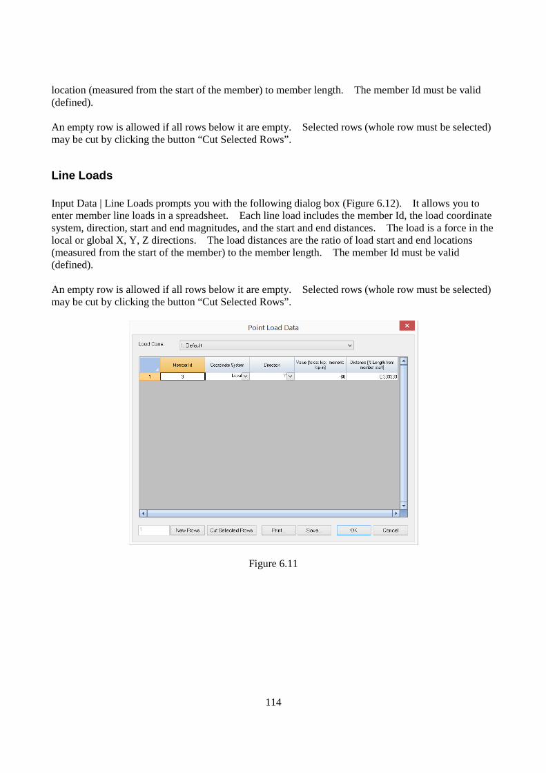
114

location (measured from the start of the member) to member length. The member Id must be valid (defined). An empty row is allowed if all rows below it are empty. Selected rows (whole row must be selected) may be cut by clicking the button “Cut Selected Rows”.

Line Loads Input Data | Line Loads prompts you with the following dialog box (Figure 6.12). It allows you to enter member line loads in a spreadsheet. Each line load includes the member Id, the load coordinate system, direction, start and end magnitudes, and the start and end distances. The load is a force in the local or global X, Y, Z directions. The load distances are the ratio of load start and end locations (measured from the start of the member) to the member length. The member Id must be valid (defined). An empty row is allowed if all rows below it are empty. Selected rows (whole row must be selected) may be cut by clicking the button “Cut Selected Rows”.

Figure 6.11

115

Figure 6.12

Area Loads Input Data | Area Loads prompts you with the following dialog box (Figure 6.13). It allows you to enter member area loads in a spreadsheet. Each area load includes four node Ids, the load coordinate system, direction, load distribution, and load magnitude. The area load may be in global X, Y or Z direction, or in local Z direction. The four nodes form a quadrilateral load area and must be in the same plane. Node-4 may also be the same as Node-1, in which case the load area is a triangle. Area loads in one or all load cases may be converted to lines loads in their respective load cases. An empty row is allowed if all rows below it are empty. Selected rows (whole row must be selected) may be cut by clicking the button “Cut Selected Rows”.

116

Figure 6.13

Surface Loads Input Data | Surface Loads prompts you with the following dialog box (Figure 6.14). It allows you to enter shell surface loads in a spreadsheet. Each surface load includes the shell Id, the load coordinate system, direction, and magnitude. The load is always a force in the local or global X, Y or Z directions. The shell Id must be valid (defined). An empty row is allowed if all rows below it are empty. Selected rows (whole row must be selected) may be cut by clicking the button “Cut Selected Rows”.

117

Figure 6.14

Thermal Loads | Member Thermal Loads Input Data | Thermal Loads | Member Thermal Loads prompts you with the following dialog box (Figure 6.15). It allows you to enter member thermal loads in a spreadsheet. Each member thermal load includes the member Id and temperature increase (magnitude). The load effect is on member longitudinal direction only. Temperature gradients on members are not considered. The member Id must be valid (defined). An empty row is allowed if all rows below it are empty. Selected rows (whole row must be selected) may be cut by clicking the button “Cut Selected Rows”.

Thermal Loads | Shell Thermal Loads Input Data | Thermal Loads | Shell Thermal Loads prompts you with the following dialog box (Figure 6.16). It allows you to enter shell thermal loads in a spreadsheet. Each shell thermal load includes the shell Id and temperature increase (magnitude). The load effect is on shell membrane direction only. Temperature gradients on shells are not considered. The shell Id must be valid (defined). An empty row is allowed if all rows below it are empty. Selected rows (whole row must be selected) may be cut by clicking the button “Cut Selected Rows”.

118

Figure 6.15

Figure 6.16

Thermal Loads | Brick Thermal Loads Input Data | Thermal Loads | Brick Thermal Loads prompts you with the following dialog box (Figure 6.17). It allows you to enter brick thermal loads in a spreadsheet. Each brick thermal load includes the brick Id and temperature increase (magnitude). The brick Id must be valid (defined).

119

Figure 6.17

An empty row is allowed if all rows below it are empty. Selected rows (whole row must be selected) may be cut by clicking the button “Cut Selected Rows”.

Self Weights The Input Data | Self Weights command is identical to the one found in the Loads menu. It is provided here for convenience only.

Calculated Masses Input Data | Calculated Masses prompts you with the following dialog box (Figure 6.18). It allows you to view the masses calculated from the load combination for frequency analysis set in Run | Frequency Analysis. The program will automatically convert all forces (not moments) in the positive or negative gravity direction to masses and apply them in all available mass degrees of freedom. Obviously, the calculated mass values cannot be modified. However, you may convert all the calculated masses to additional masses. In this case, the “Convert loads to masses” option in Run | Frequency Analysis will be turned off. This technique may be useful when you want to account for the influence of axial loads on frequencies.

Additional Masses Input Data | Additional Masses prompts you with the following dialog box (Figure 6.19). It allows you to enter additional nodal mass and nodal mass moment of inertia values. Each nodal mass or mass moment of inertia includes the node Id, the mass direction, and magnitude. The mass direction

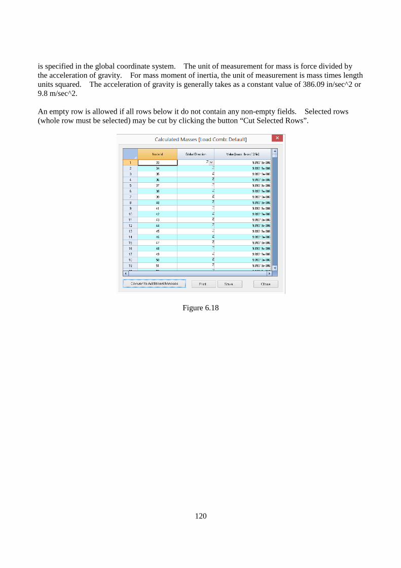
120

is specified in the global coordinate system. The unit of measurement for mass is force divided by the acceleration of gravity. For mass moment of inertia, the unit of measurement is mass times length units squared. The acceleration of gravity is generally takes as a constant value of 386.09 in/sec^2 or 9.8 m/sec^2. An empty row is allowed if all rows below it do not contain any non-empty fields. Selected rows (whole row must be selected) may be cut by clicking the button “Cut Selected Rows”.

Figure 6.18

121

Figure 6.19

Response Spectra Library Input Data | Response Spectra Library is identical to Loads | Response Spectrum Library.

Drift Nodes Input Data | Drift Nodes prompts you with the following dialog box (Figure 6.20). It allows you to enter nodes that will be used for floor drift calculation. An empty row is allowed if all rows below it do not contain any non-empty fields. Selected rows (whole row must be selected) may be cut by clicking the button “Cut Selected Rows”.

122

Figure 6.20

Comments Input Data | Comments prompts you with the following dialog box (Figure 6.21). It allows you to add or delete comments at different locations in the model. You may also add an individual comment using View | Options | Comment. A comment must be less than 256 characters in length. An empty row is allowed if all rows below it do not contain any non-empty fields. Selected rows (whole row must be selected) may be cut by clicking the button “Cut Selected Rows”.

Figure 6.21

123

Chapter 7: Analysis The Run menu provides commands to set the analysis options, to perform analysis, and to generate input and output reports. For more information on analysis, please refer to Part 3 - Technical issues.

Analysis Options Analysis | Analysis Options prompts you with the following dialog box (Figure 7.1). It allows you to set important options before performing analysis on the model. The “Model type” determines the type of the model to analyze. Model type “3D Frame & Shell” is the most general. It has all six degrees of freedom (DOFs) available to every node in the model. Any model may be analyzed with this model type. However, computer memory or time may be wasted if a simpler model can be used.

Figure 7.1

Model type “2D Frame” may be used to model a 2D frame (beams and trusses) structure in the XY plane. Only three DOFs (Dx, Dy and Doz) are available to every node in the model. The rest of the DOFs are suppressed.

124

Model type “3D Truss” may be used to model 3D truss structures. Only three DOFs (Dx, Dy, and Dz) are available to every node in the model. The rest of the DOFs are suppressed. If the model contains both 3D trusses and beams, “3D Frame & Shell” model type must be used and appropriate moment releases assigned to truss elements. Model type “2D Truss” may be used to model 2D truss structures in the XY plane. Only two DOFs (Dx and Dy) are available to every node in the model. The rest of the DOFs are suppressed. If the model contains both 2D trusses and beams, “2D Frame” model type must be used and appropriate moment releases assigned. Model type “2D Plate Bending” may be used to model 2D plate bending structures such as flat slabs or mat foundations in the XY plane. It uses only the plate bending action of the shell formulation. Only three DOFs (Dz, Dox and Doy) are available to every node in the model. The rest of the DOFs are suppressed. The self weight should be in either –Z or +Z direction depending on your sign convention for loads. Model type “2D Plane Stress” may be used to model 2D plane stress structures such as shear walls in the XY plane. It uses only the membrane action of the shell formulation. Only two DOFs (Dx and Dy) are available to every node in the model. The rest of the DOFs are suppressed. Model type “3D Brick” may be used to model 3D solid structures. Only three DOFs (Dx, Dy, Dz) are available to every node in the model. The rest of the DOFs are suppressed. You should be careful choosing an approriate Model type when mixing different types of elements. For example, if you have both 3D beams and bricks, you probably want to choose “3D Frame & Shell” Model type and then apply nodal springs with very small rotational stiffness to brick nodes to prevent instability. Non-linear convergence control includes the maximum iterations and axial force tolerance between adjacent P-Delta iterations. The maximum iterations apply to both P-Delta analysis and analysis involving non-linear springs. It is provided to avoid excessive number of nonlinear iterations during the solution. A default value of 10 is usually sufficient. Axial force tolerance between adjacent P-Delta iterations reflects the actual convergence of the P-Delta analysis. The default value of 0.5% should be good for most cases. It is a good idea to perform a linear analysis before the P-Delta analysis. In this way, you may identify any problems in the model before the more rigorous analysis option is undertaken. By default, the program considers shear deformations on members in the model. You must also set shear areas of member sections for this option to take effect. To do that, run the command Geometry | Sections. You may ignore member shear deformations by unchecking “Consider shear deformation on members”. Generally, shear deformations on members are insignificant. However, you should check this option when members are of relatively great depths. Shear deformation, when considered, applies to both the element stiffness matrix and local (segmental) deflections. The number of segments for member segmental output may be set from 1 to 127. A value of 20 segments is recommended in most cases. More segments produce more accurate results, but require more usage of computer memory. The accuracy may be reflected in the smoothness of moment, shear and deflection diagrams. Since member local deflection is computed based on the moment and

125

shear diagrams, a value of more than 20 segments may be needed if very accurate local deflection is desired. You may specify whether to use cracked section properties for the analysis. The cracking factors are specified by Input Data | Members, Input Data | Shell4s or RC Design | Cracking Factors. Cracking factors will not be applied until “Use cracked section properties (Icr) for members and finite elements” is checked here. This option is given so that you do not need to reenter cracking factors if you decide to use gross section properties in a different analysis run. Usually, stresses in finite elements are not continuous across element boundary. You may average them for adjacent shells/bricks at nodes. For “Stress averaging based on local coordinate system”, element stresses at each of element nodes are calculated by averaging nodal stresses of the elements that share the same node and that have the same local coordinate system. For “Stress averaging for all adjacent elements”, element stresses at each of element nodes are calculated by averaging nodal stresses of the elements that share the same node and that have the local coordinate system parallel to global coordinate system. Stress averaging usually makes the results more accurate and the contours smoother. However, it may also disguise insufficient convergence for an unsatisfactory (coarse) finite element mesh. Obviously, stress averaging can only apply to adjacent elements that have compatible local coordinate systems. For planar elements, stress averaging should only apply to adjacent elements that share the same local coordinate systems. Special attention should be given to shear stress averaging at supports since shears of adjacent elements may have opposite signs. By default, the program uses the MITC4 for shell bending formulation. The MITC4 is a thick plate formulation and accounts for the out-of-plane shear deformation. However, if the shell elements are all rectangular, you may use the classical Kirchhoff plate bending formulation. The Kirchhoff plate element is a thin plate formulation and ignores the out-of-plane shear deformation. For the membrane formulation of the shell element or of the brick element, incompatible modes may be added to the standard isoparametric (compatible) formulation. The incompatible shell element models the in-plane bending more accurately than the standard compatible element. The incompatible brick element, which produces much more accurate results than the compatible one, should almost always be preferred. There are three kinds of solvers available in Real3D: 64-bit floating point skyline, 128-bit floating point skyline and 64-bit floating point sparse. The 64-bit skyline solver is the standard solver similar to many analysis programs in the market. The 64-bit sparse solver is the fastest, but it lacks informative messages when something goes wrong during a solution. The sparse solver can only be used for static analysis. The 64-bit floating point (double precision)s are enough for most structures. For some large or numerically sensitive models, the 64-bit floating point (double precision)s may fail and 128-bit floating point (quad precision) provides an invaluable alternative. The 128-bit floating point (quad precision) is extremely stable and accurate, but relatively slow. It is the recommended solver if the model contains rigid diaphragms to avoid numerical difficulties. The sparse solver also has the option to use an out-of-core approach to minimize the requirement of computer memory. It is useful to solve extremely large structural models.

126

You have the option to consider rigid diaphragm actions during the solution. This is useful to ignore rigid diaphragms without deleting the existing diaphragms.

Static Analysis Analysis | Static Analysis performs the static analysis of the model. You should set the appropriate analysis options before running this command. To do that, just run the command Analysis | Analysis Options. A solver dialog box (Figure 7.2) is displayed showing the progress of the solver. The solver first solves all linear load combinations, then all nonlinear load combinations. If the model contains compression-only or tension-only springs, every load combination is a nonlinear load combination. Otherwise, only P-Delta load combinations are nonlinear. The nonlinear load combinations are solved iteratively and therefore may require considerable solution time. A log file with the extension of “log” is created during the solution process. It is always a good idea to open this file and check its messages, especially when warning or error messages appeared in the solver dialog box. You may abort the solving process by pressing ESC if a non-sparse solver is used.

Figure 7.2

Frequency Analysis Analysis | Frequency Analysis prompts you with the following dialog box (Figure 7.3). It allows you to set important options before performing frequency analysis on the model. The load combination for mass and stiffness must be specified. If you want to input nodal mass and/or mass moment of inertia directly, you may do so from Loads | Additional Masses or Input |

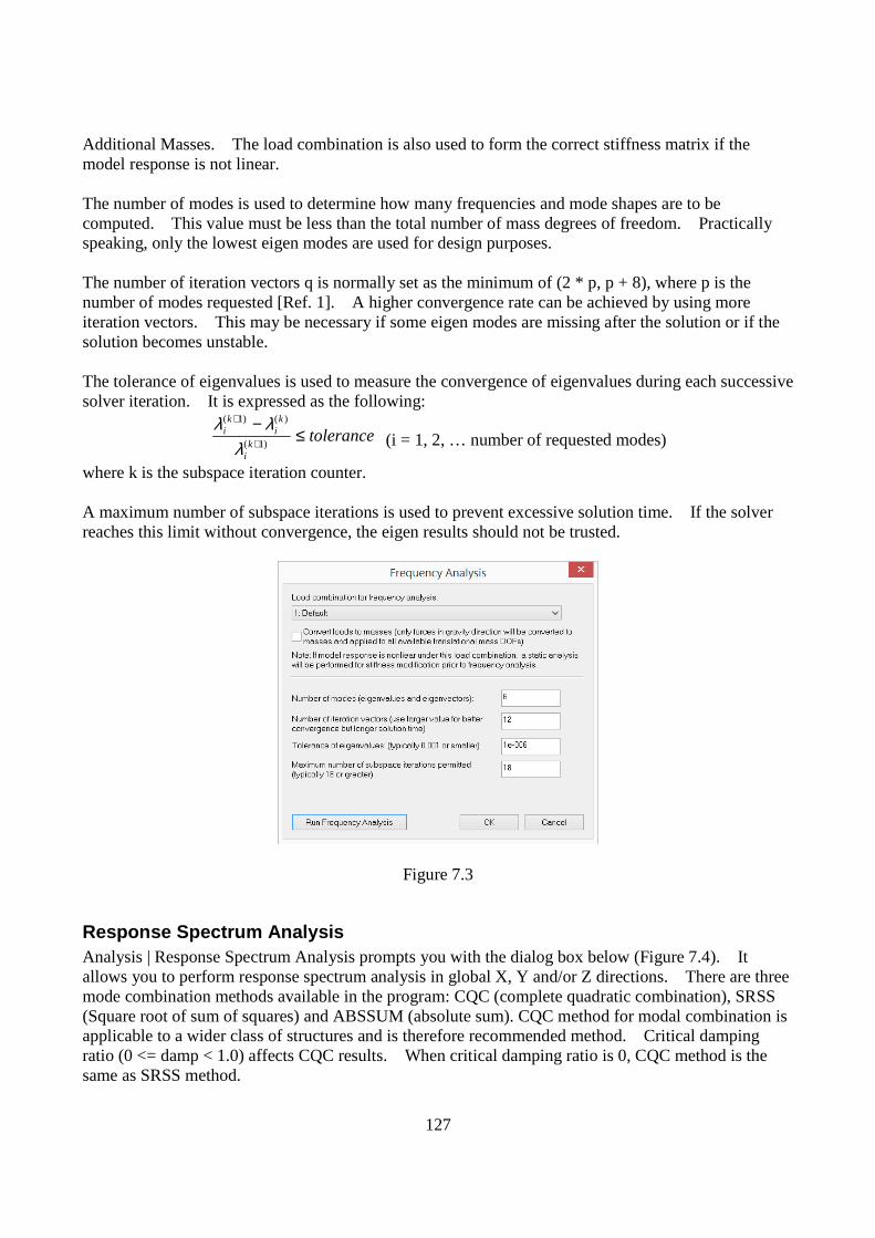
127

Additional Masses. The load combination is also used to form the correct stiffness matrix if the model response is not linear. The number of modes is used to determine how many frequencies and mode shapes are to be computed. This value must be less than the total number of mass degrees of freedom. Practically speaking, only the lowest eigen modes are used for design purposes. The number of iteration vectors q is normally set as the minimum of (2 * p, p + 8), where p is the number of modes requested [Ref. 1]. A higher convergence rate can be achieved by using more iteration vectors. This may be necessary if some eigen modes are missing after the solution or if the solution becomes unstable. The tolerance of eigenvalues is used to measure the convergence of eigenvalues during each successive solver iteration. It is expressed as the following:

tolerancek

i

ki

ki ≤

−+

+

)1(

)()1(

λλλ

(i = 1, 2, … number of requested modes)

where k is the subspace iteration counter. A maximum number of subspace iterations is used to prevent excessive solution time. If the solver reaches this limit without convergence, the eigen results should not be trusted.

Figure 7.3

Response Spectrum Analysis Analysis | Response Spectrum Analysis prompts you with the dialog box below (Figure 7.4). It allows you to perform response spectrum analysis in global X, Y and/or Z directions. There are three mode combination methods available in the program: CQC (complete quadratic combination), SRSS (Square root of sum of squares) and ABSSUM (absolute sum). CQC method for modal combination is applicable to a wider class of structures and is therefore recommended method. Critical damping ratio (0 <= damp < 1.0) affects CQC results. When critical damping ratio is 0, CQC method is the same as SRSS method.

128

You must first run from Analysis | Frequency Analysis prior to running this command. Response spectrums can be defined from Loads | Response Spectra Library or Input Data | Response Spectra Library. Inertia forces in global direction X, Y or/and Z from response spectrum analysis will be calculated and then converted to nodal loads. These nodal forces will be placed in respective load cases such as INERTIA_LOADCASE_X_MODE_1, INERTIA_LOADCASE_X_MODE_2 etc. Existing loads in these load cases will be deleted prior to the load conversion. In addition, response spectrum load combinations INERTIA_LOADCOMB_X_MODE_1, INERTIA_LOADCOMB_X_MODE_2 etc. will be created or recreated. Static analysis will be performed on spectrum load combinations (as well as normal user-defined load combinations) automatically. Modal combinations will be subsequently calculated for results such as displacements, forces and stresses etc. using CQC, SRSS or ABSSUM on the response spectrum load combinations. Normally, modal combination results are all positive due to the sign lost during SRSS, CQC and ABSSUM procedures. However, you can choose to use signage for modal combination results based on the dominant mode (with maximum participation factor) in each global direction. Modal combination results is done in each global direction first. Using directional factors, these directional modal results will be combined into final modal combination results, which can be added to any user-defined load combination results if non-zero response spectrum load factor is specified in the load combination definition (see Loads | Load Combinations).

Figure 7.4

129

Chapter 8: Analysis Result The Analysis Result menu provides commands to view and print analysis results for each load combination in spreadsheets.

Nodal Displacements Analysis Result | Nodal Displacements displays the following dialog box (Figure 8.1). It allows you to view nodal displacements for each load combination. The displacements for each node include three translational components Dx, Dy and Dz and three rotational components Dox, Doy and Doz. You have the option to view the displacements for the selected nodes only.

Figure 8.1

Story Drifts Analysis Result | Story Drifts displays the following dialog box (Figure 8.2). It allows you to view story drifts for each load combination. You have the option to view the story drifts for the selected nodes only. Note: You must first select and define Drift Nodes from Geometry | Story Drift Nodes or Input Data | Story Drift Nodes before performing static analysis.

Figure 8.2

130

Support Reactions Analysis Result | Support Reactions displays the following dialog box (Figure 8.3). It allows you to view support reactions for each load combination. The reactions for each support include three force components Rx, Ry and Rz and three moment components Rox, Roy and Roz. You have the option to view the reactions for the selected supports only. Note: The support reactions do not include multi-DOF constraint forces and moments.

Figure 8.3

Spring Reactions | Nodal Analysis Result | Spring Reactions | Nodal displays the following dialog box (Figure 8.4). It allows you to view nodal spring reactions for each load combination. The reactions for each nodal spring include three force components SRx, SRy and SRz and three moment components SRox, SRoy and SRoz. You have the option to view the reactions for the selected nodal springs only.

Figure 8.4

Spring Reactions | Coupled Analysis Result | Spring Reactions | Coupled allows you to view coupled spring reactions for each load combination. The result dialog box is identical to that of Analysis Result | Spring Reactions | Nodal.

Spring Reactions | Line Analysis Result | Spring Reactions | Line displays the following dialog box (Figure 8.5). It allows you to view line spring reactions for each load combination. The reactions for each line spring include three force components SRx, SRy and SRz. You have the option to view the reactions for the selected line springs only.

131

Figure 8.5

Spring Reactions | Surface Analysis Result | Spring Reactions | Surface displays the following dialog box (Figure 8.6). It allows you to view surface spring reactions for each load combination. The reactions for each surface spring include three force components SRx, SRy and SRz. You have the option to view the reactions for the selected surface springs only.

Figure 8.6

Multi-DOF Constraint Forces & Moments Analysis Result | Multi-DOF Constraint Forces & Moments displays the following dialog box (Figure 8.7). It allows you to view constraint forces and moments for each load combination. The value columns can be either constraint forces (for DOF X, Y and Z) or moments (for DOF OX, OY and OZ).

Figure 8.7

132

Member End Forces & Moments Analysis Result | Member End Forces & Moments displays the following dialog box (Figure 8.8). It allows you to view forces and moments at the ends of each member for each load combination. The end forces and moments include axial force Fx, major shear Fy, minor shear Fz, torsion Mx, minor moment My, and major moment Mz. You have the option to view the end forces and moments for the selected members only.

Figure 8.8

Member Segmental Results Analysis Result | Member Segmental Results displays the following dialog box (Figure 8.9). It allows you to view member segmental results for each load combination. The segmental results are shown at each segmental point designated by a distance along the member. They include axial force Fx, major shear Fy, minor shear Fz, torsion Mx, minor moment My, major moment Mz, major local deflection Dy, and minor local deflection Dz. You have the option to view the segmental forces and moments for the selected members only.

Figure 8.9

Shell4 Forces & Moments

133

Analysis Result | Shell4 Forces & Moments displays the following dialog box (Figure 8.10). It allows you to view shell forces and moments for each load combination. The shell forces and moments include in-plane normal forces Fxx, Fyy and shear force Fxy; out-of-plane bending moments Mxx, Myy, Mxy; and out-of-plane shear forces Vxx, Vyy. You may specify the force and moment locations to be at the nodes and/or the center of each shell by running Settings | Data Options. You have the option to view the forces and moments for the selected shells only.

Figure 8.10

Shell4 Principal Forces & Moments Analysis Result | Shell4 Principal Forces & Moments displays the following dialog box (Figure 8.11). It allows you to view shell principal forces and moments for each load combination. The shell principal forces and moments include in-plane principal forces Fmax, Fmin and the principal angle F-angle; out-of-plane principal moments Mmax, Mmin and the principal angle M-angle; out-of-plane principal shear force Vmax and the principal angle V-angle. You may specify the principal force and moment locations to be at the nodes and/or the center of each shell by running Settings | Data Options. You have the option to view the principal forces and moments for the selected shells only.

Figure 8.11

Shell4 Stresses [Top]

Shell4 Stresses [Bottom]

134

Analysis Result | Shell4 Stresses displays the following dialog box (Figure 8.12). It allows you to view shell top or bottom stresses for each load combination. The shell stresses include three normal components Sxx, Syy, Szz and three shear components Sxy, Sxz and Syz. You may specify the stress locations to be at the nodes and/or the center of each shell by running Settings | Data Options. You have the option to view the stresses for the selected shells only.

Shell4 Principal Stresses Analysis Result | Shell4 Principal Stresses displays the following dialog box (Figure 8.13). It allows you to view shell top or bottom principal stresses and Von Mises stresses for each load combination. You may specify the stress locations to be at the nodes and/or the center of each shell by running Settings | Data Options. You have the option to view the stresses for the selected shells only.

Figure 8.12

Figure 8.13

Shell4 Nodal Resultants Analysis Result | Shell4 Nodal Resultants displays the following dialog box (Figure 8.14). It allows you to view shell nodal resultants for each load combination. The nodal resultants are concentrated forces and moments at element nodes that keep individual elements in equilibrium. They are expressed in the local coordinate system. You have the option to view the nodal resultants for the selected shells only.

135

Figure 8.14

Brick Stresses Analysis Result | Brick8 Stresses displays the following dialog box (Figure 8.15). It allows you to view brick stresses for each load combination. The brick stresses include three normal components Sxx, Syy, Szz and three shear components Sxy, Syz and Sxz. You may specify the stress locations to be at the nodes and/or the center of each brick by running Settings | Data Options. You have the option to view the stresses for the selected bricks only.

Figure 8.15

Brick8 Principal Stresses Analysis Result | Brick Principal Stresses displays the following dialog box (Figure 8.16). It allows you to view brick principal stresses and Von Mises stresses for each load combination. Brick principal stresses are shown at locations of nodes and/or center of each shell. You may control the locations by running Settings | Data Options. Brick principal stresses include three principal components S1, S2, S3 and direction vectors (V1x, V1y and V1z) and (V3x, V3y and V3z). You have the option to view the principal stresses for selected bricks only.

136

Figure 8.16

Envelope | Nodal Displacements Analysis Result | Envelope | Nodal Displacements first displays a dialog box (Figure 8.17) for you to select load combinations for the envelope. It then displays nodal displacements envelope dialog box (Figure 8.18). The envelope includes maximum and minimum displacements and the corresponding load combination numbers. The load combination dropdown box serves as a reference so you can match load combination numbers with load combination names.

Figure 8.17

137

Figure 8.18

Envelope | Support Reactions Analysis Result | Envelope | Support Reactions first displays a dialog box (Figure 8.17) for you to select load combinations for the envelope. It then displays support reactions envelope dialog box (Figure 8.19). The envelope includes maximum and minimum reaction forces/moments and the corresponding load combination numbers. The load combination dropdown box serves as a reference so you can match load combination numbers with load combination names.

Figure 8.19

138

Envelope | Member Segmental Results Analysis Result | Envelope | Member Segmental Results first displays a dialog box (Figure 8.17) for you to select load combinations for the envelope. It then displays beam segmental results envelope dialog box (Figure 8.20). The envelope includes maximum and minimum beam segmental forces/moments and the corresponding load combination numbers. The load combination dropdown box serves as a reference so you can match load combination numbers with load combination names.

Figure 8.20

Eigenvalues Analysis Result | Eigenvalues displays the following dialog box (Figure 8.21). It allows you to view eigenvalues (λ) and their derivatives such as periods (T), frequencies (f), and circular frequencies (ω). In addition, an error measure is calculated for each eigenvalue according to the following (see Ref. 1):

Error Measure = )()(

)(1

)()(

2)(

ki

Tki

ki

qq

λ−

Where )(k

iq is the vector in the matrix )(kQ corresponding to

)(kiλ .

139

Figure 8.21

Eigenvectors Analysis Result | Eigenvectors displays the following dialog box (Figure 8.22). It allows you to view eigenvectors (mode shapes) for each mode of vibration. It is worthwhile to point out that eigenvectors are meaningful only in their relative values.

Figure 8.22

Mode Participation Factors Analysis Result | Mode Participation Factors displays the following dialog box (Figure 8.23). It allows you to view mode participation factors for each mode in global X, Y and Z directions. You must perform response spectrum analysis beforehand.

Figure 23

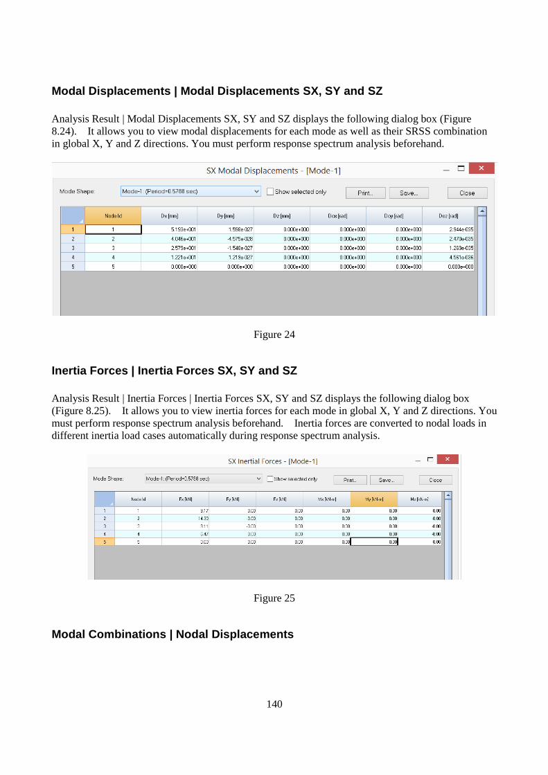
140

Modal Displacements | Modal Displacements SX, SY and SZ Analysis Result | Modal Displacements SX, SY and SZ displays the following dialog box (Figure 8.24). It allows you to view modal displacements for each mode as well as their SRSS combination in global X, Y and Z directions. You must perform response spectrum analysis beforehand.

Figure 24

Inertia Forces | Inertia Forces SX, SY and SZ Analysis Result | Inertia Forces | Inertia Forces SX, SY and SZ displays the following dialog box (Figure 8.25). It allows you to view inertia forces for each mode in global X, Y and Z directions. You must perform response spectrum analysis beforehand. Inertia forces are converted to nodal loads in different inertia load cases automatically during response spectrum analysis.

Figure 25

Modal Combinations | Nodal Displacements

141

Analysis Result | Modal Combinations | Nodal Displacements displays the following dialog box (Figure 8.26). It allows you to view nodal displacements in modal combinations (including directional combinations). You must perform response spectrum analysis beforehand.

Figure 26

Modal Combinations | Support Reactions Analysis Result | Modal Combinations | Support Reactions displays the following dialog box (Figure 8.27). It allows you to view support reactions in modal combinations (including directional combinations). You must perform response spectrum analysis beforehand. Note: The support reactions do not include multi-DOF constraint forces and moments.

Figure 27

Modal Combinations | Nodal, Coupled, Line, Surface Spring Reactions Analysis Result | Modal Combinations | Nodal, Line, Surface Spring Reactions a dialog box similar to Modal Combinations | Support Reactions above (Figure 27). You must perform response spectrum analysis beforehand.

Modal Combinations | Multi-DOF Constraint Forces & Moments Analysis Result | Modal Combinations | Multi-DOF Constraint Forces & Moments displays the following dialog box (Figure 8.28). It allows you to view multi-DOF constraint forces & moments in

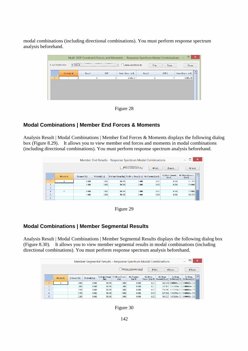
142

modal combinations (including directional combinations). You must perform response spectrum analysis beforehand.

Figure 28

Modal Combinations | Member End Forces & Moments Analysis Result | Modal Combinations | Member End Forces & Moments displays the following dialog box (Figure 8.29). It allows you to view member end forces and moments in modal combinations (including directional combinations). You must perform response spectrum analysis beforehand.

Figure 29

Modal Combinations | Member Segmental Results Analysis Result | Modal Combinations | Member Segmental Results displays the following dialog box (Figure 8.30). It allows you to view member segmental results in modal combinations (including directional combinations). You must perform response spectrum analysis beforehand.

Figure 30

143

Modal Combinations | Shell4 Forces & Moments Analysis Result | Modal Combinations | Shell4 Forces & Moments displays the following dialog box (Figure 8.31). It allows you to view shell4 forces and moments in modal combinations (including directional combinations). You must perform response spectrum analysis beforehand.

Figure 31

Modal Combinations | Brick Stresses Analysis Result | Modal Combinations | Brick Stresses displays the following dialog box (Figure 8.32). It allows you to view brick stresses in modal combinations (including directional combinations). You must perform response spectrum analysis beforehand.

Figure 32

Modal Combinations | Base Shears Analysis Result | Modal Combinations | Base Shears displays the following dialog box (Figure 8.33). It allows you to view modal base shears in X and Z directions. You can compare them with the base shears computed by equivalent lateral force procedure using relevant code such as ASCE 7-10. You must perform response spectrum analysis beforehand. Base Shears are not computed by the program if the model contains multi-DOF constraints.

144

Figure 33

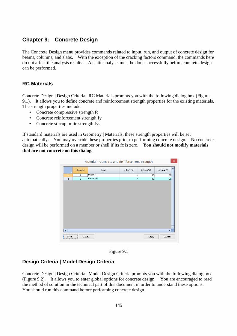
145

Chapter 9: Concrete Design The Concrete Design menu provides commands related to input, run, and output of concrete design for beams, columns, and slabs. With the exception of the cracking factors command, the commands here do not affect the analysis results. A static analysis must be done successfully before concrete design can be performed.

RC Materials Concrete Design | Design Criteria | RC Materials prompts you with the following dialog box (Figure 9.1). It allows you to define concrete and reinforcement strength properties for the existing materials. The strength properties include:

• Concrete compressive strength fc • Concrete reinforcement strength fy • Concrete stirrup or tie strength fys

If standard materials are used in Geometry | Materials, these strength properties will be set automatically. You may override these properties prior to performing concrete design. No concrete design will be performed on a member or shell if its fc is zero. You should not modify materials that are not concrete on this dialog.

Figure 9.1

Design Criteria | Model Design Criteria Concrete Design | Design Criteria | Model Design Criteria prompts you with the following dialog box (Figure 9.2). It allows you to enter global options for concrete design. You are encouraged to read the method of solution in the technical part of this document in order to understand these options. You should run this command before performing concrete design.

146

Figure 9.2

Design Code Specifies design codes. Currently the program supports ACI 318-02/05/08/11/14 only.

Column min and max reinforcement ratios

Column minimum and maximum reinforcement ratios are used to generate column sections. They should be set between 1% and 8%. For all practical purposes, the maximum reinforcement ratio should be less than 4% to avoid rebar congestion.

Neutral axis steps for accuracy

Neutral axis steps affect the solution accuracy and speed. A value of 250 ~ 500 for neutral axis steps is sufficiently accurate for most sections. The adequacy of neutral axis steps can be determined by smoothness of the P-Mx and/or P-My interaction diagrams.

Biaxial angle steps

Biaxial angle steps affects the solution accuracy and speed. For biaxial problems, steps must be multiple of 4. A value of 16 or 32 is sufficiently accurate for most sections. The adequacy of biaxial angle steps can be determined by smoothness of the Mx-My interaction diagram. For uniaxial problems, biaxial angle steps should always be set to 4. This will give P-Mx (+) at 0 degree angle, P-Mx (-) at 180 degrees angle, P-My (+) at 90 degree angle, P-My (-) at 270 degrees angle.

Axial capacity steps for display

Specifies the number of axial steps for the display of interaction diagrams / surfaces and result data in the spreadsheet. This value should be smaller than neutral axis steps. A value of 20 to 50 is usually adequate.

Exclude concrete displaced by steel

Should almost always be checked. This option is provided for verifications with textbooks only!

Always use 1.0 for Cm

If this option is checked, Cm = 1.0 will be used for all concrete columns. Otherwise, the program will compute Cm automatically based on moment curvature and the existence of transverse loading on the column.

Sustained load combination for

computing Beta-d in

Specify the load combination that contains the all sustained load cases with each case load factor equal to 1.0.

147

columns Ignore compressive

force in concrete shear capacity

Specify whether or not to ignore the increase in column concrete shear capacity due to the influence of compressive force. Axial forces are ignored on concrete beams.

Check capacity at column ends only

If this option is checked, column capacity is checked at its ends only. Otherwise, column capacity is checked at every station along the column that analysis outputs.

Compute minimum moment

If this option is checked, a minimum moment Pu * (0.6 + 0.03h) is considered for design

Automatically compute support widths

Select this option so that flexural design starts at the support faces and shear design starts at a distance of ‘d’ from the face of support.

Slab/plate min. reinf. ratios

Specify slab/plate minimum top and bottom reinforcement ratios for design. According to ACI 318-02/05/08/11/14, area of shrinkage and temperature reinforcement shall provide at least 0.18% of gross concrete area.

Design Criteria | Beam Design Criteria Concrete Design | Design Criteria | Beam Design Criteria prompts you with the following dialog box (Figure 9.3). It allows you to define and/or assign different design criteria to selected concrete beams. An Id is assigned automatically to each design criterion by the program and may not be changed. You may assign a label with 127 maximum characters to each design criterion for easy identification. The beam design criteria include:

• Number of stirrup legs. • Stirrup bar size. • Bottom and top concrete covers measured from section edge to the centroid of longitudinal

bars. You may add one or more criteria by clicking the “New Rows” button. You may also print all design criteria in the list by clicking the “Print” button. The “Assign active criteria to selected members” checkbox may be used to assign the active beam design criterion to selected beams. The active criterion refers to the one that currently has focus in the list in the dialog box. In order for beam design criteria assignments to take place, beams must be selected beforehand. The program always has a default beam design criterion labeled “Default”. You may not delete this criterion or change its label. You may however change its properties.

148

Figure 9.3

Design Criteria | Column Design Criteria Concrete Design | Design Criteria | Column Design Criteria prompts you with the following dialog box (Figure 9.4). It allows you to define and/or assign different design criteria to selected concrete columns. An Id is assigned automatically to each design criterion by the program and may not be changed. You may assign a label with 127 maximum characters to each design criterion. The column design criteria include:

• Sway flags in x and y directions. • Unbraced lengths in x and y directions. You may enter zero if you want the program to use

the member lengths as the unbraced lengths. • Effective length factors in x and y directions. • Number of tie legs. • Tie bar size. • Concrete cover to the outside surface of ties. Since different longitudinal bar sizes may be

used during automatic section generation, the program computes concrete cover to bar center based on the following formula: “cover to tie” + “tie diameter” + one half of “longitudinal bar diameter” Note: This is different from concrete cover for beams.

• Start and end bar trial sizes for section generation. • Bar layout. 0=bars will be placed on all sides of the section; 1=bars will be placed only on

the sides parallel to the section major axis; 2=bars will be placed only on the sides parallel to the section minor axis; 3=bars will be distributed equally on all sides.

• Confinement: Confining reinforcement can be either tied or spiral. Spiral applies to circular sections only.

149

Figure 9.4 You may add one or more criteria by clicking the “New Rows” button. You may also print all design criteria in the list by clicking the “Print” button. The “Assign active criteria to selected members” checkbox may be used to assign the active column design criterion to selected columns. The active criterion refers to the one that currently has focus in the list in the dialog box. In order for column design criteria assignments to take place, columns must be selected beforehand. The program always has a default column design criterion labeled “Default”. You may not delete this criterion or change its label. You may however change its properties.

Design Criteria | Plate Design Criteria Concrete Design | Design Criteria | Plate Design Criteria prompts you with the following dialog box (Figure 9.5). It allows you to define and/or assign different design criteria to selected concrete plates. An Id is assigned automatically to each design criterion by the program and may not be changed. You may assign a label with 127 maximum characters to each design criterion. The plate design criteria include:

• Bottom-x, bottom-y, top-x and top-y concrete covers measured from plate edge to the centroid of bars

You may add one or more criteria by clicking the “New Rows” button. You may also print all design criteria in the list by clicking the “Print” button. The “Assign active criteria to selected shells” checkbox may be used to assign the active plate design criterion to selected plates. The active criterion refers to the one that currently has focus in the list in the dialog box. In order for plate design criteria assignments to take place, plates must be selected beforehand.

The program always has a default plate design criterion labeled “Default”. You may not delete this criterion or change its label. You may however change its properties.

150

Figure 9.5

Design Criteria | Exclude Elements Concrete Design | Design Criteria | Exclude Elements prompts you with the following dialog box (Figure 9.6). It allows you to include or exclude concrete design for selected beams, columns, and plates. For example, you might want to exclude some plate elements (such as those near supports) from concrete design where large stress spikes are present. Plate envelope contours do not include the excluded shell elements. This makes the contour bands appear more distinct from each other.

Figure 9.6

Design Criteria | Cracking Factors Concrete Design | Design Criteria | Cracking Factors prompts you with the following dialog box (Figure 9.7). It allows you to assign cracking factors to selected beams, columns, and plates. Cracking factors apply only to bending stiffness of members and shell elements. Note: Cracking factors are not considered by the program unless you check the option “Use cracked section properties (Icr) for members and finite elements” in Run | Analysis Options. Analysis results are cleared after assignment of cracking factors.

151

Figure 9.7

Assign | Beam Design Properties Concrete Design | Assign | Beam Member Properties prompts you with the following dialog box (Figure 9.8). It allows you to continuously assign concrete beam design properties to members. After clicking “Assign”, you can start to continuously assign concrete beam design properties by window-selecting members until you right click the mouse or press the ESC key.

Figure 9.8

Assign | Column Design Properties Concrete Design | Assign | Column Member Properties prompts you with the following dialog box (Figure 9.9). It allows you to continuously assign concrete column design properties to members. After clicking “Assign”, you can start to continuously assign concrete column design properties by window-selecting members until you right click the mouse or press the ESC key.

152

Figure 9.9

Assign | Plate Design Properties Concrete Design | Assign | Plate Member Properties prompts you with the following dialog box (Figure 9.10). It allows you to continuously assign concrete plate design properties to shells. After clicking “Assign”, you can start to continuously assign concrete plate design properties by window-selecting shells until you right click the mouse or press the ESC key.

Figure 9.10

Design Input | RC Member Input Concrete Design | Design Input | RC Member Input prompts you with the following dialog box (Figure 9.11). It allows you to enter beams and columns for concrete design in a spreadsheet. Each element includes the class (“B” for beam, “C” for column), design criteria Id, cracking factor, and exclusion design flag (0 for included, 1 for excluded). The element cracking factor with a value between 0 (fully cracked) and 1 (uncracked) applies to the moments of inertia of member elements. You may not modify the member Id. Design criteria Ids must be valid (defined). Beam and column design criteria combo boxes are provided for you to correctly pick and apply proper element class and design criteria to selected members.

153

Figure 9.11

Design Input | RC Plate Input Concrete Design | Design Input | RC Plate Input prompts you with the following dialog box (Figure 9.12). It allows you to enter plates for concrete design in a spreadsheet. Each element includes design criteria Id, cracking factor, and exclusion design flag (0 for included, 1 for excluded). The element cracking factor with a value between 0 (fully cracked) and 1 (uncracked) applies to the moments of inertia of member elements. You may not modify the plate (shell) Id. Design criteria Ids must be valid (defined). Plate design criteria combo box is provided for you to correctly pick and apply proper element design criteria to selected shells.

Perform Design Concrete Design | Perform Design performs the concrete design based on the design criteria and design input. You must run the analysis successfully prior to running this command.

Design Output | RC Analysis Envelope Concrete Design | Design Output | RC Analysis Envelope displays the following dialog box (Figure 9.13). It allows you to view the negative and positive moment envelope as well as the shear envelope for concrete design. You have the option to view the envelope for the selected beams/columns only. Note: The envelope only considers the load combinations that are designated for concrete design.

154

Figure 9.12

Figure 9.13

Design Output | RC Beam Results Concrete Design | Design Output | RC Beam Results displays the following dialog box (Figure 9.14). It allows you to view top and bottom required steel for flexure and their corresponding design moments at every analysis output station along the member. You have the option to view the RC beam results for the selected beams only.

155

Figure 9.14

Design Output | RC Column Results Concrete Design | Design Output | RC Column Results displays the following dialog box (Figure 9.15). It allows you to view the final column design sections and their unity check ratios. Some intermediate results such as moment magnification factors (Mz and My-factors), Beta-d and Cm’s are output as well. You have the option to view the RC column results for the selected columns only.

Figure 9.15

Design Output | Flexural/Axial Interaction | Sections Concrete Design | Design Output | Flexural/Axial Interaction | Sections displays all column sections generated by the program based on the input of material, section and column design criteria (Figure 9.16).

156

Figure 9.16

Design Output | Flexural/Axial Interaction | P-Mx (+) Concrete Design | Design Output | Flexural/Axial Interaction | P-Mx (+) displays the P-Mx result data in a spreadsheet, with positive moment about the section major axis (at biaxial angle of 0 degree) (Figure 9.17).

Figure 9.17

157

Design Output | Flexural/Axial Interaction | P-Mx (-) Concrete Design | Design Output | Flexural/Axial Interaction | P-Mx (-) displays the P-Mx result data in a spreadsheet, with negative moment about the section major axis (at biaxial angle of 180 degrees).

Design Output | Flexural/Axial Interaction | P-My (+) Concrete Design | Design Output | Flexural/Axial Interaction | P-My (+) displays the P-My result data in a spreadsheet, with positive moment about the section minor axis (at biaxial angle of 90 degrees).

Design Output | Flexural/Axial Interaction | P-My (-) Concrete Design | Design Output | Flexural/Axial Interaction | P-My (-) displays the P-My result data in a spreadsheet, with negative moment about the section minor axis (at biaxial angle of 270 degrees).

Design Output | Flexural/Axial Interaction | P-Mx-My Concrete Design | Design Output | Flexural/Axial Interaction | P-Mx-My displays the P-Mx-My result data in a spreadsheet at each biaxial angle step and axial capacity step.

Design Output | Flexural/Axial Interaction | Print Diagrams Concrete Design | Design Output | Flexural/Axial Interaction | Print Diagrams allows you to view and print the interaction diagrams for each column section (Figure 9.18). The red and blue lines are the interaction diagrams about section major and minor axes respectively. A sketch of the section and the key control points are listed above the diagrams as well.

158

Figure 9.18

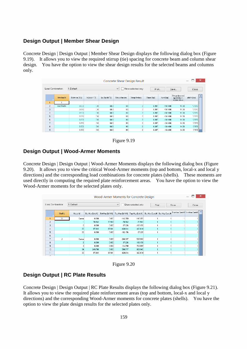
159

Design Output | Member Shear Design Concrete Design | Design Output | Member Shear Design displays the following dialog box (Figure 9.19). It allows you to view the required stirrup (tie) spacing for concrete beam and column shear design. You have the option to view the shear design results for the selected beams and columns only.

Figure 9.19

Design Output | Wood-Armer Moments Concrete Design | Design Output | Wood-Armer Moments displays the following dialog box (Figure 9.20). It allows you to view the critical Wood-Armer moments (top and bottom, local-x and local y directions) and the corresponding load combinations for concrete plates (shells). These moments are used directly in computing the required plate reinforcement areas. You have the option to view the Wood-Armer moments for the selected plates only.

Figure 9.20

Design Output | RC Plate Results Concrete Design | Design Output | RC Plate Results displays the following dialog box (Figure 9.21). It allows you to view the required plate reinforcement areas (top and bottom, local-x and local y directions) and the corresponding Wood-Armer moments for concrete plates (shells). You have the option to view the plate design results for the selected plates only.

160

Figure 9.21

Diagrams| RC Member Envelope Diagram Concrete Design | Diagrams | RC Member Envelope Diagram displays the following dialog box (Figure 9.22). It allows you to view the required flexural reinforcement as well as the moment and shear envelope used for designing concrete beams. It also allows you to view required stirrup or tie spacing for concrete beams and columns. You have the option to view the member envelope diagrams for the selected members only.

Figure 9.22

Diagrams | RC Plate Envelope Contour Concrete Design | Diagrams | RC Plate Envelope Contour displays the following dialog box (Figure 9.23). It allows you to view the required flexural reinforcement as well as the Wood-Armer moments (top and bottom, local x and y directions) for concrete plates (shells). You have the option to view the plate envelope contours for the selected plates only.

161

Figure 9.23

RC Report Concrete Design | RC Report displays the following dialog box (Figure 9.24). It allows you to print concrete design report on beams and columns. You have the options to include flexural design for concrete beams, axial-flexural design for concrete columns as well as shear design for concrete beams and columns. You also have the option to print the report on selected members only. Figure 9.25 shows the print preview for a column axial-flexural design report.

Figure 9.24

162

Figure 25

163

RC Tools | Rebar Database Concrete Design | RC Tools | Rebar Database displays the following dialog box (Figure 9.26). It allows you to select different rebar databases for use in concrete design.

Figure 9.26

RC Tools | K Calculator Concrete Design | RC Tools | K Calculator (Figure 9.27) allows you to accurately calculate effective length factors (braced and unbraced Ks) based on the beam and column relative stiffness input.

Figure 9.27

164

RC Tools | Quick R-Beam Flexural Design Concrete Design | RC Tools | Quick R-Beam Flexural Design (Figure 9.28) allows you to quickly design a rectangular concrete beam according to ACI 318-02/05/08/11/14. Minimum reinforcement may be optionally computed. You have the option to design the rectangular beam as singly or doubly reinforced. A negative reinforcement area means the design fails.

Figure 9.28

RC Tools | Quick T-Beam Flexural Design Concrete Design | RC Tools | Quick T-Beam Flexural Design (Figure 9.29) allows you to quickly design a concrete tee beam according to ACI 318-02/05/08/11/14. Minimum reinforcement may be optionally computed. The tee beam is always designed as singly reinforced. A negative reinforcement area means the design fails.

Figure 9.29

165

Chapter 10: Steel Design

Steel Materials Steel Design | Design Criteria | Steel Materials prompts you with the following dialog box (Figure 10.1). It allows you to define steel strength properties for the existing materials. The strength properties include:

• Steel yield stress Fy • Steel rupture stress Fu

If standard materials are used in Geometry | Materials, these strength properties will be set automatically. You may override these properties prior to performing steel design. No steel design will be performed on a member if its modulus is not close (within 10%) to 29E3 ksi. You should not modify materials that are not steel on this dialog.

Figure 10.1

Design Criteria | Model Design Criteria Steel Design | Design Criteria | Model Design Criteria prompts you with the following dialog box (Figure 10.2). Use Direct Design Method currently only affects how the moment magnification factor B1 (small p-delta effect along member length) is calculated. You also have the option not to consider moment magnification factor B1 altogether. Please be advised that P-Delta analyses should be performed on load combinations that are used for steel design. To be conservative, you can always use 1.0 for Cm that accounts for nonuniform moment. Uncheck the “Alwsys use 1.0- for Cm” if you would like the program to calculate Cm for automatically.

166

Figure 10.2

You have the option to only use sections defined in Steel Design | Design Criteria | Section Pool during the design process. This is useful if you do not want the program to use too many steel section sizes for the entire model. Connector distance for double angles is used for sections that are double angles. The default number of section candidates designed for each member is 10. You can also specify limits for total load deflection and live load deflection.

Design Criteria | Member Design Criteria Steel Design | Design Criteria | Member Design Criteria prompts you with the following dialog box (Figure 10.3). It allows you to define and assign design criteria for members. An Id is assigned automatically to each design criterion by the program and may not be changed. You may assign a label with 127 maximum characters to each design criterion. The column design criteria include:

• Section Prefix, which is a comma delimited list. For example, if you want the member section to be with W10 or W12 size, enter the prefix as “w10,w12”. You can also specify the prefix as the exact AISC shapes. Use the prefix “Default” if you do not want the member section changed from the original shape.

• Sway flags in x and y directions. These flags are currently only used in checking the validity of Kx and Ky.

• The length between points that are braced against lateral displacement of compression flange Lb. Currently, the program only supports equal Lb along the member length. For non-

167

continuously braced, the program will use the member length for Lb if the value is entered 0. For continuously braced, 0 must be entered for Lb.

Figure 10.3

• Lateral-torsional buckling modification factor for non-uniform moment diagrams Cb. The program will automatically calculate Cb if the value is entered 0. You can always use Cb = 1.0 for conservative reasons.

• Unbraced lengths in x, y and z directions. You may enter zero if you want the program to use the member lengths as the unbraced lengths. Please note that x, y directions refer to strong and weak axes in steel design.

• Effective length factors in x, y and z directions. • You have the option to set the maximum unity check ratio. By default, this ratio is 1.0. You

can set a value less than 1.0 (but greater than 0.0) for conservative reasons.

Design Criteria | Section Pool Steel Design | Design Criteria | Section Pool prompts you with the following dialog box (Figure 10.4). It allows you to define a list of sections that may be used exclusively for design. You can copy a list of section labels from the AISC table. You can also enter sections manually. Each line in the section pool box can only contain one section. Furthermore, you can automatically add all the section candidates to the section pool (from Steel Design | Design Result).

168

Figure 10.4

Design Criteria | Exclude Elements Steel Design | Design Criteria | Exclude Elements prompts you with the following dialog box (Figure 10.5). It allows you to include or exclude steel design for selected members.

Figure 10.5

Assign Member Design Properties Steel Design | Assign Member Design Properties prompts you with the following dialog box (Figure 10.6). It allows you to continuously assign steel design properties to members. After clicking “Assign”, you can start to continuously assign steel design properties by window-selecting members until you right click the mouse or press the ESC key.

Figure 10.6

169

Design Input | Steel Member Input Steel Design | Design Input | Steel Member Input prompts you with the following dialog box (Figure 10.7). It allows you to enter members for steel design in a spreadsheet. Each element includes the design criteria Id, and exclusion design flag (0 for included, 1 for excluded). You may not modify the member Id. Design criteria Ids must be valid (defined). Steel design criteria combo box is provided for you to correctly pick and apply proper steel design criteria to selected members.

Figure 10.7

Perform Design The Steel Design | Perform Design menu allows you to run the steel design.

Design Result The Steel Design | Design Result allows you to view the steel design results (Figure 10.8). It also allows you to update member sections. The section column on Figure 10.8 includes a combobox that contains the member original section (first entry in the combobox) and designed section candidates (second or more entries in the combobox). You can change the member sections by picking the proper section candidates. Please be advised you need to re-analyze and design after one or more member sections are updated. The Critical Ratio and Load Combination list the highest ratio, corresponding load combination and distance considering Axial & Bending, Shear, and Deflection for all load combinations. When critical ratio on a member is controlled by deflections, you may need to update the analysis section in order to continue section design.

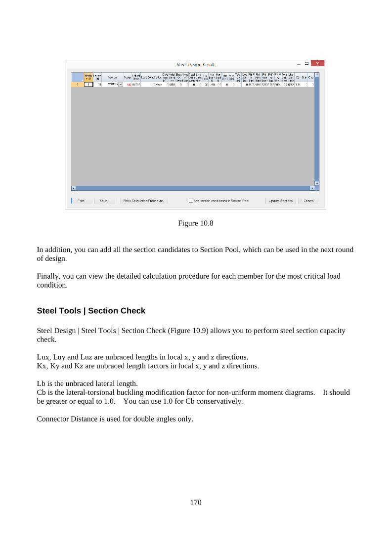
170

Figure 10.8

In addition, you can add all the section candidates to Section Pool, which can be used in the next round of design. Finally, you can view the detailed calculation procedure for each member for the most critical load condition.

Steel Tools | Section Check Steel Design | Steel Tools | Section Check (Figure 10.9) allows you to perform steel section capacity check. Lux, Luy and Luz are unbraced lengths in local x, y and z directions. Kx, Ky and Kz are unbraced length factors in local x, y and z directions. Lb is the unbraced lateral length. Cb is the lateral-torsional buckling modification factor for non-uniform moment diagrams. It should be greater or equal to 1.0. You can use 1.0 for Cb conservatively. Connector Distance is used for double angles only.

171

Figure 10.9

Pu, Mux, Muy, Vux, Vuy are required axial, major moment, minor moment, major shear and minor shear. For Pu, the compressive force is positive while tensile force is negative. Moment Mux is positive when section top most fiber is under compression. Moment Muy is positive when section rightmost fiber is under compression. Moment magnification may be optionally considered to account for the P-delta (P-δ) effect. If direct design method is chosen, the program will calculate stiffness reduction parameter based on Eq. C2-2a and C2-2b of the code. Cmx, Cmy are coefficients accounting for non-uniform moments when computing moment magnification. You can use 1.0 for Cmx and Cmy conservatively. If Cmx or Cmy is 0, 1.0 is used in the computation instead. Results include axial capacity (phi-Pn), moment capacity (phi-Mnx, phi-Mny), shear capacity (phi-Vnx, phi-Vny), moment magnification factors (B1x, B1y) and critical ratio. The section is deemed safe to resist a load if the critical ratio is less than 1.0, otherwise, the section is deemed unsafe. Please note that for single angle, the moment capacity is given about the principal axes (w-w and z-z).

172

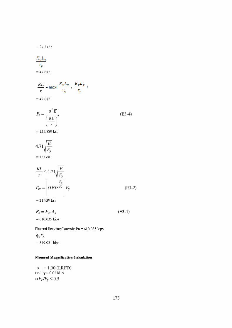
173

174

175

176

177

178

179

Steel Tools | Section Design Steel Design | Steel Tools | Section Design (Figure 10.10) allows you to quickly design steel sections against a set of load effects. The Section Design input and output are shown below:

Figure 10.10

For Section Filter Criteria, you can use either Section Prefixes or section dimension limits (but not both). The section prefixes is a comma delimited list such as W12, W14. If section prefixes is used, the section dimension limits will be ignored. If a section dimension limit is zero, then that limit criteria is ignored. By default, a maximum of ten section candidates will be provided after a successful design. You can then view the detailed check for each of the section candidate.

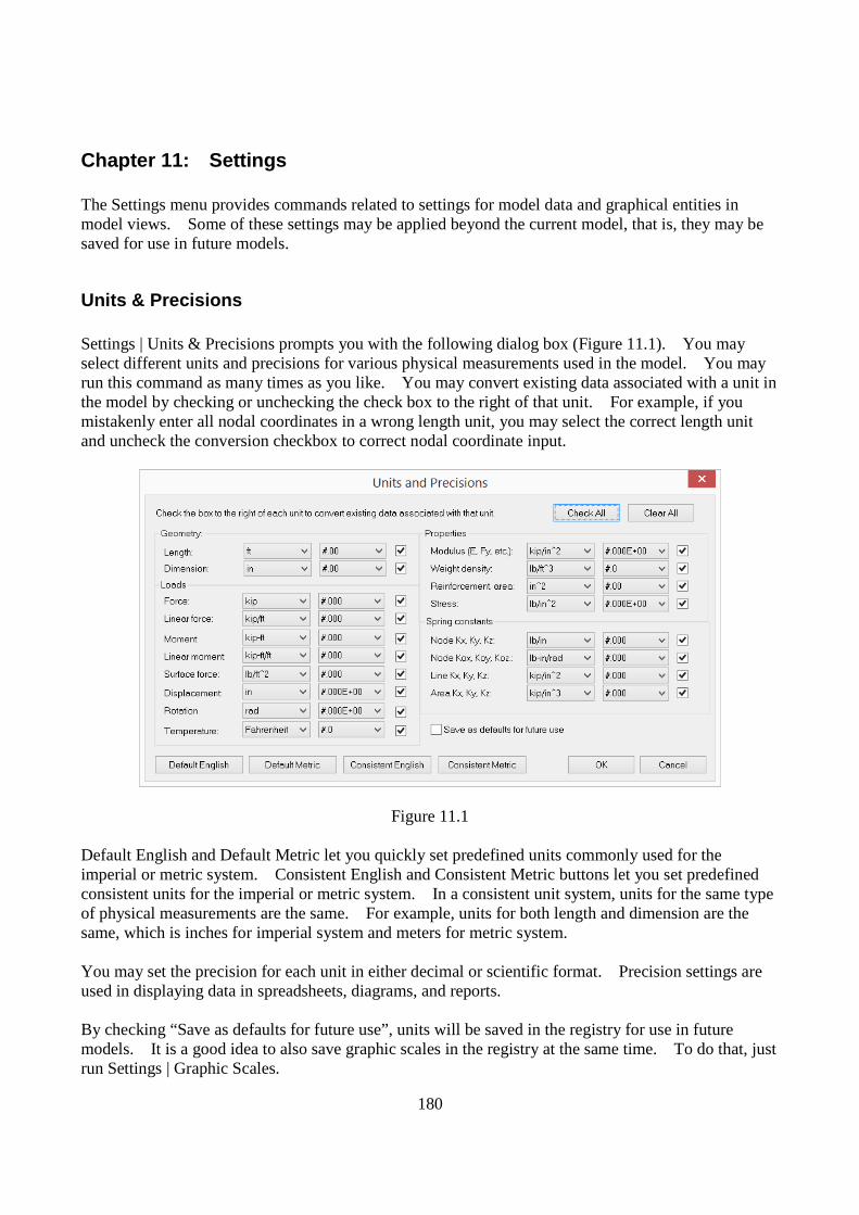
180

Chapter 11: Settings The Settings menu provides commands related to settings for model data and graphical entities in model views. Some of these settings may be applied beyond the current model, that is, they may be saved for use in future models.

Units & Precisions Settings | Units & Precisions prompts you with the following dialog box (Figure 11.1). You may select different units and precisions for various physical measurements used in the model. You may run this command as many times as you like. You may convert existing data associated with a unit in the model by checking or unchecking the check box to the right of that unit. For example, if you mistakenly enter all nodal coordinates in a wrong length unit, you may select the correct length unit and uncheck the conversion checkbox to correct nodal coordinate input.

Figure 11.1 Default English and Default Metric let you quickly set predefined units commonly used for the imperial or metric system. Consistent English and Consistent Metric buttons let you set predefined consistent units for the imperial or metric system. In a consistent unit system, units for the same type of physical measurements are the same. For example, units for both length and dimension are the same, which is inches for imperial system and meters for metric system. You may set the precision for each unit in either decimal or scientific format. Precision settings are used in displaying data in spreadsheets, diagrams, and reports. By checking “Save as defaults for future use”, units will be saved in the registry for use in future models. It is a good idea to also save graphic scales in the registry at the same time. To do that, just run Settings | Graphic Scales.

181

Data Options Settings | Data Options prompts you with the following dialog box (Figure 11.2). Distance tolerance is used for distance comparisons in certain commands such as Edit | Merge Nodes and Edit | Explode Members. Distances less than distance tolerance are considered zero by the program. The “Undo/redo levels” sets the maximum undo/redo levels which the program will perform. The program requires extra computer memory for each undo/redo level. The default undo levels setting is 100. Depending on your computer memory and model sizes, you may want to set undo levels to be smaller.

Figure 11.2

Round-off epsilon is used to truncate floating point numbers such as those found in results. For example, a fixed support may have a displacement of 1.077e-10 when in fact it should zero. A round-off epsilon of 1e-9 will do just that. Stresses are computed at the center and at the nodes of finite elements such as shells or solids. However, you may request the program to show stresses at the finite element center only, nodes only, or both. The checkbox “Show only selected entities in spreadsheet” determines if all or selected nodes, elements and their dependents will be shown in the spreadsheet. By checking this checkbox, you may easily query selected entities in a large model. It is important to point out that data in some input

182

spreadsheets may not be modified when this option is checked. The checkbox “Save results when the document is saved” gives you the option to save results (when available) to a file when the model input data is saved. The result file is a binary file and has the same file name as model input file, but with an extension of “rst” (static results) or “dyn” (dynamic results). The result file could be much larger than the model input file. The fictitious oz stiffness factor is used to multiply the minimum of diagonal terms (excluding oz) in the shell stiffness matrix to construct the fictitious oz stiffness terms. The smaller this factor, the more accurate the solution, especially for very thin and doubly curved shells. The valid range for this factor is [1e-12, 1e-3]. You normally do not need to change its default value (1e-7). Numerical difficulties may arise during solution if this value is set too small. The diaphragm stiffness factor is used to control the diaphragm rigidity. The larger this factor, the more rigid the diaphragm action is. The valid range for this factor is [0, 1e20]. The default value is 1e4. Numerical difficulties may be present during static or frequency analysis if the diaphragm stiffness factor is set too large (say 1e13 for 64-bit floating point solver). It is generally recommended to use 128-bit floating point solver to avoid the aforementioned problem.

New Origin Settings | New Origin prompts you with the following dialog box (Figure 11.3). It allows you to reset the model origin. In particular, the origin may be set at the current model center. This allows you to center the model so its view may be rotated more smoothly.

Figure 11.3

Vertical Axis Settings | Vertical Axis prompts you with the following dialog box (Figure 11.4). It allows you to set either global Y (default) or global Z as the vertical axis for the model. Vertical axis has impact on the preset views such as front/back, left/right, top/bottom and isometric views. It also affects the way real time rotation works.

183

Figure 11.4

Graphic Scales Settings | Graphic Scales prompts you with the following dialog box (Figure 11.5). You may set scales for graphical entities such as loads, nodes, supports etc. By “Save as defaults for future use”, these scales will be saved in the registry for future uses. It is a good idea to save units to the registry at the same time. To do that, run Settings | Units & Precisions.

Figure 11.5

Colors Settings | Colors prompts you with the following dialog box (Figure 11.6). It allows you to set colors of different graphical entities in the model. You may modify the color(s) of one or more items at a time. By checking “Use color cues for different materials”, concrete, steel and wood materials will show different colors in rendering mode. By checking “Use white background for image captures”, a white background will be used for the captured image even if a different background color is used in the model views. This option will reduce the amount of ink required to print the images. Color settings can be optionally saved to the registry for future use.

184

Figure 11.6

Preferences Settings | Preferences prompts you with the following dialog box (Figure 11.7). The “Data Folder” determines the default folder or directory when a file is saved or opened. The “Automatic file backup period” determines how frequently the model files are saved automatically. Enter 0 for no auto-backups. Backup files have the extension “r3a.r3a”. Settings for “Response Animation” can be set here. You may activate the Response Animation command from the View menu after an analysis has been performed successfully. You have the options to lock the model after analysis is performed successfully. By default, an internal HTML viewer is used to view text and graphical reports. You may use an external HTML viewer such as Internet Explorer instead. You have the option to save drawing grid settings. By default, rubber-banding is enabled while drawing beams, shells or bricks. You may want to disable this feature if your computer graphic card is not fully OpenGL compatible. Additional settings related to filling shear and moment diagrams, the font for graphics and the spreadsheet appearance are available. When the sparse solver is used for static analysis, you may choose an out-of-core approach so computer memory usage is minimized. You may specify the maximum amount of memory to be used in the out-of-core sparse solver. This value should be smaller than the physical memory available in your system. You may also specify the number of CPUs for the sparse solver. Preferences are always saved in the registry for future use.

185

Figure 11.7

Enable/Disable Hardware Acceleration Settings | Enable/Disable Hardware Acceleration allows you to turn on or off OpenGL hardware acceleration. By default, OpenGL hardware acceleration is turned on. If you encounter graphics problems (due to faulty graphics drivers) in the software, you may want to try to disable hardware acceleration. The graphics performance may degrade significantly but should be acceptable on most modern systems. This command may also be useful when using virtual Windows on Mac machine.

Tools | Unit Conversion Settings | Tools | Unit Conversion displays a tool for conversion between various units (Figure 11.8).

Figure 11.8

186

Tools | Calculator Settings | Tools | Calculator displays the Windows Calculator.

Tools | Text Editor Settings | Tools | Text Editor displays the Windows Notepad.

Tools | Copy Command History Settings | Tools | Copy Command History copies the history in the command window to the clipboard. You may then paste the command history content to a text editor using Ctrl + V. A command history is associated with each open document.

Tools | Clear Command History Settings | Tools | Clear Command History clears the history in the command window. You may want to copy the command history before running this command.

Toolbars | Main Toolbar Settings | Toolbars | Main Toolbar shows or hides the main toolbar.

Toolbars | View Toolbar Settings | Toolbars | View Toolbar shows or hides the toolbar that contains commands for controlling the view.

Toolbars | Edit/Run Toolbar Settings | Toolbars | Edit/Run Toolbar shows or hides the toolbar related to edit, analysis, and result visualization commands.

Toolbars | Input Toolbar Settings | Toolbars | Input Toolbar shows or hides the toolbar that contains input buttons.

Toolbars | Output Toolbar Settings | Toolbars | Output Toolbar shows or hides the toolbar that contains output buttons.

187

Toolbars | Command Bar Settings | Toolbars | Command Bar shows or hides the command window.

Toolbars | Status Bar Settings | Toolbars | Status Bar shows or hides the status bar.

188

Chapter 12: Window The Window menu provides commands to create new windows and arrange existing windows. In this program, a window may be used interchangeably with a view. The program has two types of views: model view and report view. The model view contains the graphical display of the input in a model. The report view contains text or graphical report in html format for the input or output of a model.

New Window Window | New Window creates a new window or view based on the current view. You may create different model views with different display settings with respect to zooming, panning, loading diagram, shear or moment diagrams, contours, etc. For example, you may have one model view to display moment diagram, another view to display shear diagram. You may create as many views as you want. However, too many views may clutter the view area and make graphic display sluggish.

Close Window | Close closes the current window.

Close All Window | Close All closes all windows that are currently open. You will be prompted to save file(s) if necessary.

Tile Horizontal Window | Tile Horizontal arranges all opened windows horizontally.

Tile Vertical Window | Tile Vertical arranges all opened windows vertically.

Tile Cascade Window | Cascade arranges all opened windows in an overlapped manner

.

189

Technical Issues

190

Chapter 13: Coordinate Systems Two kinds of coordinate systems are used in the program, namely, the global coordinate system and the local coordinate system. The global coordinate system is the one and only fixed Cartesian system in a structural model. The local coordinate system applies to each individual member or finite element.

Global Coordinate System The global coordinate system is a fixed Cartesian system that is used for entire model. The three axes are denoted by capital letters X, Y and Z. They follow the right-hand rule. By default, that is, when a model is not rotated for viewing purpose, the X axis points from left to right (horizontal), the Y axis points from bottom to top (vertical), and the Z axis points from screen to out of screen (perpendicular to screen). The global coordinate system is used in the following input:

- nodal coordinates, nodal loads - degrees of freedom related to nodes, supports and springs - self weights - point, line, and surface loads on members and finite elements [may also be specified in the

element local coordinate system] The global coordinate system is used in the following output:

- nodal displacements - support and spring reactions - brick stresses

Local Coordinate Systems - General Each member or finite element has a local coordinate system. It is a Cartesian system that has a default orientation (when local angle equals 0) and may be changed at any time. The three axes are denoted by small letters x, y, z. They follow the right-hand rule. The local coordinate system exists to facilitate input and output for member and finite elements. For example, point or line loads on a member may be most conveniently specified in the local coordinate system of the member. The element results such as shears and moments are output in the local coordinate system for design purposes. Since the local coordinate systems directly affect input and results, it is always prudent to check them for correctness using the commands such as View | Annotate or Render. You may change the local coordinate systems using the commands such as Edit | Element Local Angle or Reverse Element Nodes’ Order. It may be worthwhile to note that it is the directional vectors that matter while the origin of the local coordinate system is insignificant in this program.

191

The local coordinate system is used in the following input: - point, line, and surface loads on members and finite elements [may also be specified in the

global coordinate system] - member moment releases

The local coordinate system is used in the following output:

- member forces, moments, and local deflections - shell forces, moments, and stresses

In the following sections, Vx, Vy and Vz represent the local x, y, and z vectors respectively. VX, VY and VZ represent the global X, Y, and Z vectors respectively. For vector algebra, please refer to relevant math textbooks.

Member Local Coordinate System The local coordinate system of a member is determined by the start and end nodes, and an element local angle. The default (local angle equals 0 degrees) local coordinate system of a member is defined using the following procedures:

Steps Description Mathematical Notations A Vx points from node 1 (N1) to node 2 (N2) Vx = N2 – N1 B1 For vertical members:

Vz is always parallel to VZ

For vertical members Vz = VZ

B2 For non-vertical members: Vz is perpendicular to a plane formed by Vx and VY

For non-vertical members Vz = Vx x VY

C Vy is determined based on Vx and Vz and the right-hand rule

Vy = Vz x Vx

For a member with a non-zero local angle (γ), first follow the procedures above that determine the default local coordinate system. Then rotate the default system a γ angle about its local x vector Vx. The rotated Vx, Vy and Vz define the local coordinate system. Figure 13.1 shows the local coordinate systems of some members with different local angles (γ). For maximum flexibility, the program allows you to auto-calculate and assign a local angle to each of the selected members such that its local z axis is perpendicular to the plane formed by the two member end points and a user-defined 3rd point. The local x axis stays the same. The local y axis is determined by the local x and z axes using right hand rule. This can be useful for some models such as a dome where member webs are in plane with the member ends and the center of the sphere.

192

Local coordinate systems for members with different local angles

Figure 13.1

Four-Node Shell Local Coordinate System The local coordinate system of a shell is determined by its four nodes, and an element local angle. The default (local angle equals 0 degrees) local coordinate system of a four-node shell is defined based on the shape of the shell element.

Rectangular Shell Non-Rectangular Shell

193

For rectangular shells, the default local coordinate system is easily defined by the following: local x points from N1 to N2, local y points from N1 to N4 and local z is perpendicular to the shell surface. For non-rectangular shells, the default local coordinate system is defined using the following procedures:

Steps Description Mathematical Notations

A Local z is perpendicular to the shell surface Let V1 = N2 – N1, Let V2 = N4 – N1

Vz = V1 x V2

B1 For horizontal shells that are parallel to global XZ

plane, local x is parallel to global X

For horizontal shells Vx = VX

B2 For non-horizontal shells, Vx is perpendicular to a

plane formed by global Y and local z For non-horizontal shells

Vx = VY x Vz

C Vy is determined based on Vx and Vz and the

right-hand rule Vy = Vz x Vx

For a shell with a non-zero local angle (γ), first follow the procedures above that determine the default local coordinate system. Then rotate the default system a γ angle about is its local z vector Vz. The rotated Vx, Vy and Vz define the local coordinate system. Figure 13.2 shows the local coordinate systems of some shell elements with different local angles (γ)

Local coordinate systems for shells with different local angles

Figure 13.2

194

Eight-Node Brick Local Coordinate System The local coordinate system for a brick element is always identical to the global coordinate system. It is fixed and cannot be changed.

195

Chapter 14: Nodes Nodes are numbered points in space. They are used to define the geometry and connectivity of all members and finite elements in a model. For members, a node is sometimes referred to as a joint, which has a physical meaning of the intersection of two members such as a beam and a column. However, in this program, the term “node” is generally preferred because it carries a more general meaning.

Nodal Coordinates The location of a node is defined by the global X, Y, and Z coordinates. Since each member or finite element connects to two or more nodes, nodal coordinates define the geometry of a model. For example, when you move an element, you actually move the locations of the nodes connected to that element.

Degrees of Freedom (DOFs) Each node may have a maximum of six global degrees of freedom (DOFs) associated with it. They are three translational DOFs along the global X, Y, Z directions (Dx, Dy and Dz) and three rotational DOFs about the global X, Y, Z directions (Dox, Doy and Doz). Some of these DOFs may not be available depending upon the type of a model. For example, the model type “2D Truss” has Dx and Dy available and Dz, Dox, Doy, Doz unavailable or suppressed; while the model type “2D Plate Bending” only has Dz, Dox, Doy available and Dx, Dy, Doz suppressed. You may always use the model type “3D Frame and Shell” to analyze any structure, however, time and computer memory may be wasted if a simpler model type can be used instead. You may choose the appropriate model type by command Run | Analysis Options. Six nodal displacements associated with 6 DOFs are output for each node. For restrained or unavailable DOFs, the program outputs the corresponding displacements as zero. Nodal displacements should be the first thing to check for when determining result correctness since the solution is displacement-based. If the displacements are wrong, nothing else will be correct.

Node Numbers A distinct integral number is assigned to each node. Node numbers are used to define the connectivity of member and finite elements. Duplicate numbers in nodes are not permitted. There can be gaps in node numbering sequence. The program will automatically renumber the nodes internally before performing the solution. The order of node numbering in a model is insignificant to the final results, but it may affect the time and computer memory required to solve the model. For a very large model, node renumbering may be important in order to reduce the half band width in the global stiffness matrix and therefore the solution time. You may renumber the nodes sequentially based on nodal coordinates using the command Edit | Renumber Nodes.

196

Half Band Width (HBW) is defined as [Ref.7] as follows: { )min(maxmax

1elel

mel

dofdofHBW −=≤≤

where m is the total number of structural elements, and the eldofmax and eldofmin are the maximum and minimum global degrees of freedom numbers associated with element el. For example, in Figure 14.1 and 14.2, models A and B are identical 3D frames (6 DOFs per node) but with different node numbering schemes. Model A has a HBW of 6 * (9 + 1) = 60 while model B has a HBW of 6 * (5 + 1) = 36. Therefore, model B is more economical than model A because of the reduction of half band width.

Model A: HBW=60

Figure 14.1

Model B: HBW=36

Figure 14.2

Loads Forces or moments may be applied to a node. These forces and moments are specified in the global coordinate system. You may regard enforced displacements as special kinds of loads. They are specified in supports

Supports By default, a node is unrestrained, that is, it is free to move in any of the six available DOFs. However, for a model to be stable, restraints on one or more DOFs must be imposed on some nodes. Restraints may be rigid or flexible. Rigid restraints are referred to as supports while flexible restraints are referred to as springs. You may regard supports as springs with infinite spring constants.

197

You may assign a support with one or more DOFs (Dx, Dy, Dz, Dox, Doy and Doz) restrained to a node. The program uses a six-character code to represent restraint conditions of a support in six DOFs. For example, “111111” represents a fixed a support while “111000” represents a pinned support. By default, restrained DOFs have zero enforced displacements. You may specify non-zero enforced displacements to any or all of restrained DOFs. The enforced displacements are discarded if they are assigned to unrestrained DOFs. You may regard these enforced displacements as special kinds of loads. They participate in all load combinations but always with a load factor of 1.0. The forces or moments required to enforce rigid restraints are called support reactions. They are computed by the program.

Multi-DOF Constraints We can also apply constraints to one or more nodes. A constraint is achieved through the following constraint equation in Real3D:

Q1 * constraint factor 1 = Q2 * constraint factor2

Where Q1 and Q2 are nodal displacements (translational or rotational) at one or two nodes. If the constraint is applied to the same node, the constraint DOFs must be different. Constrained DOFs must be compatible: Q1 and Q2 must be both translational or rotational. Constraint factors must be non-zero. A regular support and multi-DOF constraints may be applied on the same node as long as the support/constrained directions do not interfere with each other. Multi-DOF constraints are useful in many situations. For example, we can use a constraint to model an inclined roller support by selecting appropriate constrained DOFs and constraint factors. Real3D directly supports inclined rollers on XY, YZ and XZ planes. The forces or moments required to enforce multi-DOF constraints are called multi-DOF constraint forces and moments. They are computed by the program and are listed separately from the regular support reactions.

Nodal Springs Springs are flexible restraints. Springs applied to nodes are referred to as nodal springs. You may assign a nodal spring to a node with one or more global DOFs (Dx, Dy, Dz, Dox, Doy and Doz) restrained. To qualify to be a valid flexible restraint, the corresponding spring constant must be specified. A restraint may be designated as linear, compression-only or tension only. A compression-only restraint is active only when the nodal displacement in the restrained direction is negative. A tension-only restraint is active only when the nodal displacement in the restrained direction is positive. If a model contains one or more compression-only or tension-only springs, the whole problem becomes nonlinear and the solution becomes iterative for each load combination.

198

Coupled Springs Real3D also implements an advanced spring type called coupled spring. A coupled spring is defined with 6 x 6 symmetric stiffness terms. A nodal spring is a special coupled spring with only diagnonal terms specified. Coupled springs are useful in modeling and simplifying sub-structures such as bridge foundations. The forces or moments required to enforce the flexible restraints are called spring reactions. They are computed by the program.

199

Chapter 15: Members A member is a two-node straight frame element with a constant cross section. The term “frame element”, “beam element”, and “member” are used interchangeably in this program. The truss element is a special frame element with moments fully released at both ends. The frame element formulation accounts for axial, torsional, and bending about strong and weak axes, with options to include shear deformations and axial stress stiffening (P-Delta) effects. Moment releases may be applied to either or both ends of the element. The frame element may be used to model continuous beams, 2D or 3D frames, 2D or 3D trusses or a mixture of two. The program provides powerful commands to generate commonly used framed structures such as continuous beams, 2D or 3D frames, arc beams, and non-prismatic beams. A non-prismatic member is approximated by subdividing the original member into several prismatic members. You may run these commands from the Generate menu.

Member Sections Each member must have a section assigned to it. The section properties include:

- A: axial section area - Ay: shear area along the member local y direction - Az: shear area along member the local z direction - Izz: moment of inertia about strong the local axis z - Iyy: moment of inertia about weak the local axis y - J: torsional moment of inertia

Ay and Az may be zero, in which case, the program ignores shear deformations of the element. Mathematically speaking, the program interprets them as being infinite. For rectangular sections, Ay = Az = 5/6A. For solid circular sections, Ay = Az = 0.9A. For thin-walled hollow circular sections, Ay = Az = 0.5A. For wide flange sections, Ay = web area, Az = area of two flanges [Ref. 6]. To consider member shear deformation, you must choose the proper option from the command Run | Analysis Options. Shear deformation, when considered, applies to both element stiffness and local deflections.

Local Coordinate System Each member has its own local coordinate system. The element local coordinate systems are used in element stiffness formulations. They are also used for inputs such as loads and releases and outputs such as internal shears and moments. For the definition of the member local coordinate system, refer to Chapter 13: Coordinate Systems.

Member Numbers A distinct integral number is assigned to each member. Duplicate numbers in members are not permitted. There can be gaps in the member numbering sequence. The order of member numbering

200

in a model is insignificant to the results or solution time. You may renumber the members sequentially using the command Edit | Renumber Members.

Beams Vs. Trusses By default, a member or frame element is a beam. However, if you choose the model type to be either “2D Truss” or “3D Truss”, then the frame element becomes a truss element. The program automatically assigns appropriate moment releases to all members, and suppresses all three rotational DOFs Dox, Doy, Doz for each and every node. For the model type “2D Truss”, the program also suppresses translational DOF Dz. Generally speaking, if a model contains only 2D or 3D truss elements, you should choose the model type as “2D Truss” or “3D Truss”. If a model contains both trusses and beams, you should choose the model type“2D Frame” or “3D Frame & Shell”, and assign appropriate moment releases to individual beams. A truss member is a beam with major and minor moment releases at both ends, as well as torsional moment release at either one end (but not both ends) of the member. You may choose the appropriate model type by running the command Run | Analysis Option.

Elastic Stiffness Matrix Total number of DOFs of a member is the summation of DOFs of the two nodes. Therefore, for a 3D beam, the stiffness matrix is of size 12 x 12. The elastic stiffness matrix in the local coordinate system with shear deformation is given [Ref. 8] as follows:

∆∆∆

∆∆∆

++

−

−−+−+

−−−−

−−

=

2

2

2

2

2

2

1

1

1

1

1

1

11

22

22

2

12

1

11111

22222

22

222

2

12

112

1

2

2

2

2

2

2

1

1

1

1

1

1

)4(

0)4(

00)/(

0/60/12

/6000/12

00000/

)2(000/60)4(

0)2(0/6000)4(

00)/(00000)/(

0/60/12000/60/12

/6000/120/6000/12

00000/00000/

z

y

x

z

y

x

z

y

x

z

y

x

z

y

x

z

y

x

z

y

x

z

y

x

GLJ

LL

LL

LEA

L

L

GLJGLJ

LLLL

LLLL

LEALEA

M

M

M

F

F

F

M

M

M

F

F

F

θθθ

θθθ

βαβα

ββββ

βαββαβαββα

ββββββββ

where: )1(2 ν+= E

G ; 21

12

LGA

EI

y

z=α ; 22

12

LGA

EI

z

y=α ; L

EI z

)1( 11 α

β+

= ; L

EI y

)1( 22 α

β+

=

Geometric Stiffness Matrix When a tensile axial force is present in a member, the bending stiffness of that member is increased. Conversely, when a compressive axial force is present in a member, the bending stiffness of that member is reduced. The stiffness matrix that reflects this kind of stress stiffening effect is called the geometric stiffness matrix [Ref. 3, 7]. It is determined by the element geometry and stress conditions, and is independent of the elastic properties. The geometric stiffness matrix is very effective in

201

accounting for the P-Delta effect and is implemented in the program. It may also be used to perform buckling analysis of the structure but is not implemented in the program directly. Like the elastic stiffness matrix, the geometric stiffness matrix is of size 12 x 12 and is given [Ref. 3, 7] as follows:

∆∆∆

∆∆∆

−

−−−

−−−−

−

=

2

2

2

2

2

2

1

1

1

1

1

1

2

2

22

22

2

2

2

2

2

2

1

1

1

1

1

1

15/2

015/2

000

010/05/6

10/0005/6

000001

30/00010/015/2

030/010/00015/2

000000000

010/05/600010/05/6

10/0005/6010/0005/6

000001000001

z

y

x

z

y

x

z

y

x

z

y

x

z

y

x

z

y

x

z

y

x

z

y

x

L

L

L

L

LLL

LLL

LL

LL

L

P

M

M

M

F

F

F

M

M

M

F

F

F

θθθ

θθθ

where P is the average of the axial forces (positive in tension, negative in compression) at the member ends. When the linear static (first order) analysis is chosen, the member stiffness matrix is the elastic stiffness matrix. When the P-Delta (second order) analysis option is chosen, the member stiffness matrix is the summation of the elastic stiffness matrix and the geometric stiffness matrix. You may set the appropriate analysis option with the command Run | Analysis Options

Moment Releases By default, a member is rigidly connected to two end nodes. You may however assign moment releases to either end of a member. It is important to note that the releases are applied to the member local coordinate system. The moment releases may be in major bending direction (Doz) , minor bending direction (Doy), and torsional direction (Dox). For stability reason, torsional moment release can only be applied to one end (not both ends) of a member. The element stiffness matrix is modified to enforce moment releases. A truss member is a beam with major and minor moment releases at both ends, as well as torsional moment release at either one end (but not both ends) of the member.

Tension/Compression Only By default, a member is linear. You may assign nonlinearity (linear, tension only or compression only) to the selected members. The member stiffness will be ignored if a tension only member is subjected to compressive forces or if a compression only member is subjected to tensile forces. The presence of tension or compression members makes the model nonlinear and iterative solution is required for each load combination.

202

Rigid Links A rigid link is a member that has very large sectional properties (A, Ay, Az, Iz, Iy and J). There can only be one rigid link section defined in the model and it must be named as “RIGID_LINK”. The properties for the RIGID_LINK section must be set to 0’s on the member section dialog box. The program will appropriately calculate A, Ay, Az, Iz, Iy and J during the solution process. Self weight for rigid links will be ignored by the program.

Rigid Diaphragms Rigid diaphragms may be used instead of plate finite elements to model stiff in-plane actions such as concrete floors. Internally, the program creates multiple in-plane rigid links for each diaphragm prior to static or frequency analysis. A rigid link is simply a member with very large sectional properties that can be adjusted with the diaphragm stiffness factor (see Settings | Data Options). The larger the diaphragm stiffness factor, the stronger the in-plane rigid diaphragm action is. The presence of rigid links with large diaphragm stiffness factor (say 1E10) could create numerical difficulties during the solution if 64-bit floating point solver is used. However, the unique 128-bit floating point solver in Real3D makes this problem nonexistent in that much larger diaphragm stiffness factor (say 1E20) may be used without creating numerical difficulties during solution. The program further provides the option to ignore the rigid diaphragm actions as an analysis option (Run | Analysis Options). It is important to point out that rigid diaphragm actions in the program does not use master-slave nodes.

Loads Point loads or line loads may be applied to a member. Point loads may be forces or moments. Line loads must be forces. You may specify loads in either the global or local coordinate system. The locations of loads must be in ratios of the member length, measured from the start of the member. Figure 15.1 shows examples of point and line loads. The self weight of members may be calculated automatically if the material weight densities and self weight multiplier are nonzero. By default, self weight acts in the negative global Y direction. You may however change the direction to positive or negative direction of the global X, Y, or Z. This flexibility is useful in some circumstances. For example, if you model a grillage on the XY plane, the self weight may be either in the positive or negative global Z direction, depending on your preference on load sign convention. To activate automatic self weight calculation, use the command Load | Self Weights

203

Point Loads Line Loads

local y force, distance=0.6

local y force, start distance=0,end distance=1

local z moment, distance=0.4

global Y force, stat distance=0.2, end distance=0.8

Figure 15.1

An area load may be applied to multiple members on a whole planar area. The area is defined by three or four coplanar nodes. The area load is then distributed as line loads to perimeter members of enclosed sub-areas within the load area prior to static or dynamic solution. Area loads are distributed to perimeter members that form each of the enclosed sub-areas according to the following methods:

- Two-way (rectangular sub-areas) - Short-Sides (rectangular sub-areas) - Long-Sides (rectangular sub-areas) - AB-CD Sides (rectangular sub-areas) - BC-AD Sides (rectangular sub-areas) - Centroid-based - Circumference-based

The first five distribution methods apply to four-node rectangular sub-areas only. The centroid-based method may be applied to convex sub-areas only. The circumference-based method may be applied to both convex and concave sub-areas. Loads may also be distributed to sides parallel to AB-CD or BC-AD sides of the load area. The program is intelligent enough to determine the most appropriate load distribution if inconsistencies arises. For example, if you select two-way distribution method to a sub-area that is not rectangular, the program will use the centroid-based method if the sub-area is convex or the circumference-based method if the sub-area is concave. The program allows you to convert area loads to line loads directly and automatically. This feature allows you to see how exactly the program would distribute area loads to members prior to the solution. Of course, you can always undo the conversion if you want to keep the area loads. For more information on the load conversion, please see Input Data | Area Loads… As an example, let’s say we have a 3.5 x 1.5 ft rectangular sub-area subjected to 100 lb/ft^2. The following line loads (Figure 15.2) are converted from the same area load based on different distribution methods.

204

Two-way Distribution

Short-side Distribution

Long-side Distribution

Centroid-based Distribution

Circumference-based Distribution

Figure 15.2

Area loads may be specified in either the local or global coordinate system. Global area loads may be in the global X, Y, or Z direction. Local area loads may only be in the local z direction, which is perpendicular to the load area. It is recommended that area loads be defined in their own load cases. In this way, you will find it easier to identify, edit, and delete area loads later on. There are a few limitations to the area load concept in the program. The first limitation is that the sub-areas must be close-formed by perimeter members. In the following Figure 15.3, the sub-area

205

formed by node 97, 98, 104 and 103 is not a closed sub-area because there is no member connecting the node 97 and 98. As a result, no area loading will be distributed to the three perimeter members from the sub-area. The second limitation is that sub-areas must not overlap. In Figure 15.3, the sub-areas in node 101, 102, 120 and 119 are overlapping. This will result more load being distributed to the members in these sub-areas. The program gives a warning when the area load footprint is not equal to the total actual loaded area. The problem may be solved by splitting members 119-108, 107-120 and 113-114 at the intersection point.

Figure 15.3

The third limitation is that any sub-area may not contain more than one concave node (with internal angle more than 180 degrees). The fourth limitation is that any sub-area may not contain the same node more than once in forming the perimeter polygon. The program offers automatic generation of live load patterning (point and line loads only). The following example (Figure 15.4) shows how the program generates load patterning on a five-span continuous beam. Loads on each generated pattern reside in a separate load case automatically generated. Additional load combinations are generated as needed as well.

All Spans

Odd Spans

206

Even Spans

Second Support + Alternate Spans

Third Support + Alternate Spans

Fourth Support + Alternate Spans

Fifth Support + Alternate Spans

Figure 15.4

The program also offers automatic generation of moving loads (point loads only). The mechanism employed by the program is similar to the live load patterning. Thermal loads may be applied to members. Currently, Real3D considers thermal effect in longitudinal direction. It does not consider thermal gradients in members.

Line Springs Springs are flexible restraints. Springs applied to members are referred to as line springs. You may assign a line spring to a member with one or more global DOFs (Dx, Dy and Dz) restrained. To qualify as a valid flexible restraint, the corresponding spring constant must be specified. A restraint may be designated as linear, compression-only or tension only. A compression-only restraint is active only when the nodal displacement in the restrained direction is negative. A tension-only restraint is active only when the nodal displacement in the restrained direction is positive. If a model contains one or more compression-only or tension-only springs, the whole problem becomes nonlinear and the solution becomes iterative for each load combination

207

The forces or moments required to enforce the flexible restraints are called spring reactions. They are computed by the program.

Internal Forces and Moments The program outputs internal forces and moments at designated stations along the member length. You may specify the number of segments ranging from 1 to 127 for member output by running the command Run | Analysis Options. For smooth moment and shear diagrams, the program may add extra segments. Figure 15.5 shows the positive direction of the internal forces and moments of members.

Forces Moments

Axial Force Vx

Torsion Mx

Major Shear Vy

Major Moment Mz

Minor Shear Vz

Minor Moment My

Figure 15.5

Figure 15.6 is an alternative way to show the positive direction of the internal shears and moments on the local xy and xz planes.

208

Moment & shear on the local xy plane Moment & shear on the local xz plane

Figure 15.6

209

Chapter 16: Shells A shell is a structure or part of a structure which has a relatively small thickness in comparison with the other two dimensions. A general shell forms a curved surface in space. When it forms a flat surface, it is also called a plate. In this program, when the term “plate” is used, it refers to flat shell in the out-of-plane bending action. The shell element in the program is a four-node (quadrilateral) element that combines the in-plane membrane action and the out-of-plane bending action. The in-plane membrane action is a standard isoparametric compatible formulation with the option to add incompatible modes. The out-of-plane bending action is a thick-plate formulation, with the option to use the thin-plate formulation when the element is rectangular. The element can be used to model both flat-surface plates and curved-surface general shells. Applications of shell elements in structures are wide and far-reaching. Examples are concrete floors, mat foundations, shear wall, folded plates, barrel vaults, cooling towers, spherical domes, water tanks, etc. The program provides powerful commands to generate these and other commonly used plate and shell structures. These commands include Geometry | Generate Shell4s, Edit | Extrude, Revolve, etc.

For many years, a great number of papers have been published on the subject of plate and shell structures. Although the membrane action of a shell element is relatively simple, the (plate) bending action is much more complex. Many plate elements have been proposed, some of which have been implemented in commercial programs. However, most of these proposed plate elements are either ineffective or unreliable. One of the main hurdles is known as transverse “shear locking”, that is, elements behave too stiff with respect to shear deformation especially when elements are thin or geometrically distorted. One of the few reliable plate elements is a rectangular thin plate element developed by O.C. Zienkiewicz [Ref. 2]. It is based on the Kirchhoff thin plate bending theory in which a line straight and normal to the mid-surface of the plate before loading is assumed to remain straight and normal to the deformed mid-surface after loading. The transverse shear strain is therefore assumed to be zero. This plate element is important in that it is the first plate element that can be applied reliably in engineering practice. Prior to this, plate analysis depended mainly on very few “closed-form” solutions of simple geometry and boundary conditions, and other very approximate methods such as equivalent frame method of ACI [Ref. 12]. The Kirchhoff rectangular thin plate is implemented in the program. It produces results that converge to “closed-form” solutions as finite element meshes are refined. The element, however, has to be rectangular in shape and does not account for shear deformation. A much more reliable and effective plate bending element is the MITC4 developed by K.J. Bathe and others [Ref. 1]. It is a thick plate that is based on Mindlin plate theory in which a line straight and normal to the mid-surface of the plate before loading is assumed to remain straight but not necessarily normal to the deformed mid-surface after loading. The element considers shear as well as bending deformations and may be used for both thick and thin plates. This plate element differs from earlier Mindlin theory based plate elements in that different (mixed) interpolations are used to account for the bending and transverse shear strains. The MITC4 plate bending element is implemented in the program. It is free from “shear locking” and performs well even when element meshes are distorted.

210

The shape of the element may be any general quadrilateral as long as the aspect ratio is within a reasonable range (say 0.2 to 5.0).

Shell Thicknesses Each shell must have a thickness assigned to it. Based on the ratio of thickness to span length, you may choose to use the thin or thick plate bending formulation. The thick plate formulation is generally recommended over the thin plate formulation because it applies equally well to both thick and thin plates. The program therefore uses the thick plate formulation by default. If thickness to span ratio is less than 1/20 and elements are rectangular, you may use the thin plate formulation. The thickness should be compared to the support distances, not to the sizes of individual plate elements. It is important to point out that out-of-plane shear forces exist in thin plates even though shear deformations are not considered. You may draw an analogy between a plate and a beam. A thin plate is analogous to a Euler-Bernoulli beam while a thick plate is analogous to a Timoshenko beam. We consider shear deformation for the Timoshenko beam but not for the Euler-Bernoulli beam, while shear forces exist in both the Euler-Bernoulli and Timoshenko beams.

Local Coordinate System Each shell element has its own local coordinate system. The element local coordinate systems are used in element stiffness formulations. They are also used for inputs such as loads and outputs such as internal shears, moments, and stresses. Local angles for rectangular shells must be 0s if thin plate bending formulation is used in the analysis options. For definition of the shell local coordinate system, refer to Chapter 13: Coordinate Systems.

Shell Numbers A distinct integral number is assigned to each shell. Duplicate numbers in shells are not permitted. There can be gaps in shell numbering sequence. The order of shell numbering in a model is insignificant to the results or solution time. You may renumber the shells sequentially using the command Edit | Renumber Shells.

Element In-Plane Stiffness Matrix The in-plane element formulation accounts for Dx and Dy of the local coordinate system. The in-plane stiffness matrix of the element is based on the standard isoparametric formulation [Ref 1, 2, 3]. However, when the element is rectangular in shape, incompatible modes may be optionally added to the formulation [Ref. 3]. An incompatible element, when applied, yields results of high quality especially when used to model in-plane bending. Full two by two numerical integration is used to calculate the in-plane stiffness matrix of the element.

211

Element Out-of-Plane Stiffness Matrix Out-of-plane bending accounts for Dz, Dox and Doy of the local coordinate system. By default, the MITC4 thick plate formulation is used [Ref. 1]. If the thin plate option is chosen, elements with rectangular shapes will be calculated based on the Kirchhoff thin plate formulation [Ref. 1]. Full two by two numerical integration is used in either case to calculate the out-of-plane stiffness matrix of the element.

Combining Element In-Plane and Out-of-Plane Stiffness Matrices The shell element stiffness matrix is the combination of the in-plane and out-of-plane stiffness matrices. In order to avoid singularity of the stiffness matrix, a very small “fictitious” stiffness is added to the diagonal term associated with the local DOF Doz.

Loads Surface loads may be applied to a shell. You may specify loads in either the global or local coordinate system. Surface loads are lumped to element nodes before solution. The self weight of shells may be calculated automatically if the material weight densities and self weight multiplier are nonzero. By default, the self weight acts in the negative global Y direction. You may, however, change the direction to positive or negative direction of the global X, Y or Z. This flexibility is useful under certain circumstances. For example, if you select the model type “2D Plate Bending”, the self weight may be either in positive or negative global Z direction, depending on your preference on the sign convention. To activate automatic self weight calculation, use the command Load | Self Weights. Thermal loads may be applied to shells. Currently, Real3D considers thermal effect in membrane direction. It does not consider thermal gradients in shells.

Surface Springs Springs are flexible restraints. Springs applied to shells are referred to as surface springs. You may assign a surface spring to a shell with one or more global DOFs (Dx, Dy and Dz) restrained. To qualify as a valid flexible restraint, the corresponding spring constant must be specified. A restraint may be designated as linear, compression-only or tension only. A compression-only restraint is active only when the nodal displacement in the restrained direction is negative. A tension-only restraint is active only when the nodal displacement in the restrained direction is positive. If a model contains one or more compression-only or tension-only springs, the whole problem becomes nonlinear and the solution becomes iterative for each load combination. The forces or moments required to enforce flexible restraints are called spring reactions. They are computed by the program. Surface springs may be used to model Winkler mat foundations. It may be worthwhile to note that in modeling a mat foundation, surface spring constants are the soil subgrade moduli while surface spring reactions are the soil pressures.

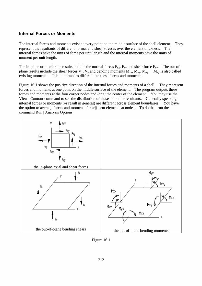
212

Internal Forces or Moments The internal forces and moments exist at every point on the middle surface of the shell element. They represent the resultants of different normal and shear stresses over the element thickness. The internal forces have the units of force per unit length and the internal moments have the units of moment per unit length. The in-plane or membrane results include the normal forces Fxx, Fyy and shear force Fxy. The out-of-plane results include the shear forces Vx, Vy and bending moments Mxx, Myy, Mxy. Mxy is also called twisting moments. It is important to differentiate these forces and moments Figure 16.1 shows the positive direction of the internal forces and moments of a shell. They represent forces and moments at one point on the middle surface of the element. The program outputs these forces and moments at the four corner nodes and /or at the center of the element. You may use the View | Contour command to see the distribution of these and other resultants. Generally speaking, internal forces or moments (or result in general) are different across element boundaries. You have the option to average forces and moments for adjacent elements at nodes. To do that, run the command Run | Analysis Options.

the in-plane axial and shear forces

the out-of-plane bending shears

the out-of-plane bending moments

Figure 16.1

213

Based on the internal forces and moments, the program computes the internal stresses at the shell bottom (the –z side) and top (the +z side) as follows. The stresses are expressed in the local coordinate systems. The stress directions correspond to the in-plane normal axial forces and shear, and the out-of-plane shears.

2

6

t

M

t

F xxxxxx +=σ (@ bottom) or 2

6

t

M

t

F xxxxxx −=σ (@ top)

2

6

t

M

t

F yyyyyy +=σ (@bottom) or 2

6

t

M

t

F yyyyyy −=σ (@ top)

2

6

t

M

t

F xyxyxy +=σ (@bottom) or 2

6

t

M

t

F xyxyxy −=σ (@ top)

t

Vxxz =σ

t

Vyyz =σ

The program also outputs in-plane principal forces and angles, and out-of-plane principal forces, moments, and angles. In addition, principal stresses S1, S2, and S3 are computed based on the stresses

xyyyxx σσσ ,, as follows:

221 )

2(

2 xyyyxxyyxxS σ

σσσσ+

−+

+=

222 )

2(

2 xyyyxxyyxxS σ

σσσσ+

−−

+=

03 =S The Von Mises stress, which is often used to estimate the yield of ductile materials, is then computed as follows:

2

)()()( 232

231

221 SSSSSS

MisesVon

−+−+−=σ

Membrane Nodal Resultants The membrane nodal resultants of a shell are concentrated forces Fx and Fy (Unit: Force) at the four nodes of each shell element. They in effect keep each individual element in equilibrium (in-plane). They are expressed in the local coordinate system. You may view nodal forces of selected shell elements by View | Annotate. The membrane nodal forces may be used to compute shears, axial forces, or moments in a shear wall. For example, the following three shells represent a pier in a shear wall. Each shell is 1.5 x 1.5 ft in size. Membrane nodal resultants Fx and Fy are shown in the first and second rows respectively at each corner of the element. The shear, axial force and moment resultants on the top of the pier may be computed as follows:

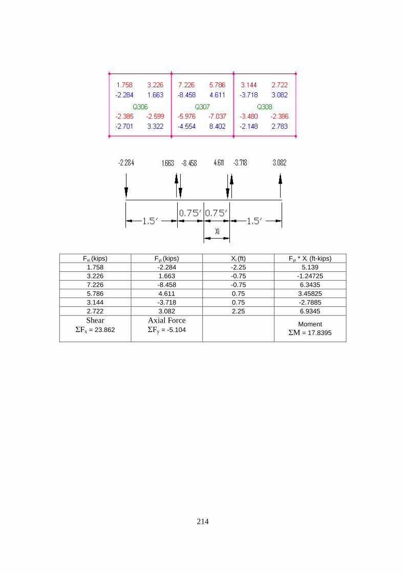
214

Fxi (kips) Fyi (kips) Xi (ft) Fyi * Xi (ft-kips) 1.758 -2.284 -2.25 5.139 3.226 1.663 -0.75 -1.24725 7.226 -8.458 -0.75 6.3435 5.786 4.611 0.75 3.45825 3.144 -3.718 0.75 -2.7885 2.722 3.082 2.25 6.9345 Shear

ΣFx = 23.862

Axial Force ΣFy = -5.104

Moment ΣM = 17.8395

215

Chapter 17: Solids The Solid element in the program is an eight-node (also called Brick) element based on isoparametric compatible or incompatible formulation [Ref 1, 2, 3]. It may be used to model structures where actions in all three dimensions are significant.

Local Coordinate System The local coordinate systems for all solids are the same. They are identical to the global coordinate system. The element nodal connectivity must be numbered in such a way so that the normal vector of the surface 1-2-3-4 points to the surface 5-6-7-8 (Figure 17.1). This is to avoid negative diagonals in the element stiffness matrix. You may use the command Edit | Reverse Element Nodes’ Order if the normal vector is not in accordance with the requirement. For more information about the brick local coordinate system, refer to Chapter 13: Coordinate Systems.

solid element

Figure 17.1

Solid Numbers A distinct integral number is assigned to each solid. Duplicate numbers in solids are not permitted. There can be gaps in solid numbering sequence. The order of solid numbering in a model is insignificant to the results or solution time. You may renumber the solids sequentially using the command Edit | Renumber Bricks.

Element Stiffness Matrix The element formulation accounts for Dx, Dy and Dz of the local coordinate system. The element stiffness matrix is based on isoparametric compatible or incompatible formulation [Ref 1, 2, 3]. Therefore, the stiffness matrix is of size 24 by 24. Full two by two numerical integration is used to calculate the stiffness matrix.

216

Loads Loads on solid elements must be input as nodal loads. The self weight of solids may be calculated automatically if material weight densities and self weight multiplier are nonzero. By default, the self weight acts in the negative global Y direction. You may however change the direction to positive or negative direction of the global X, Y or Z. To activate automatic self weight calculation, use the command Load | Self Weights Thermal loads may be applied to solid elements.

Internal Stresses Three normal stresses σxx, σyy , σzz and three shear stresses σxy, σxz, σyz are computed by the program. They are output at the eight nodes and/or at the center of the element. The program also outputs principal stresses S1, S2, S3 and the corresponding directional vectors (V1x, V1y, V1z) and (V 3x, V 3y, V 3z). The Von Mises stress, which is often used to estimate the yield of ductile materials, is then computed as follows:

2

)()()( 232

231

221 SSSSSS

MisesVon

−+−+−=σ

217

Chapter 18: Static Analysis The stiffness (or displacement-based) method is used in the solution of the structural model. The following outlines the major analysis steps:

• The individual element stiffness matrix [k] is computed in the element local coordinate system. • Based on the element nodal connectivity, [k] is transformed to the global coordinate system and

assembled into the global stiffness matrix [K]. • The load vector [R] for each load combination is formed. • The equation [K] [U] = [R] is solved for the nodal displacements [U]. • Other structural responses such as internal forces and moments are computed based on the

nodal displacements.

Load Cases and Load Combinations Each of the nodal loads, point loads, line loads, surface loads, and self weights must be assigned to a load case. The enforced displacements of supports are special loads and are considered in each load combination. The load cases are used as bases for the load combinations and are not solved directly. If you desire to solve for a particular load case, you may form a load combination with a unit load factor for that load case and 0s for all other load cases. P-Delta analyses may be performed on one or more load combinations.

Linear, Non-linear Static Analyses The program is capable of performing linear and nonlinear static analyses. The linear analysis may be applied to models where structural responses such as the displacements are expected to be linearly related to the applied loads. Otherwise the nonlinear analysis must be applied. The program currently handles two types of nonlinearity: the element nonlinearity when compression-only springs or tension-only springs are present, and the geometric nonlinearity which is commonly known as the P-Delta effect. The P-Delta effect refers to the axial stress influence on the element bending stiffness. Generally, a tensile axial force increases the element bending stiffness while a compressive axial force reduces the element bending stiffness. The P-Delta effect exists in both members and shell elements. However, the program only accounts for the P-Delta effect on members. The program assigns each load combination to be linear or nonlinear just before analysis is performed. If a model includes one or more nonlinear elements (compression-only springs or tension-only springs), the entire problem becomes nonlinear, that is, all load combinations are assigned to be nonlinear. If there are no nonlinear elements present in the model, only the P-Delta load combinations are set to be nonlinear while the rest of load combinations are linear. The non-linear load combinations must be solved iteratively and therefore are potentially time consuming. Analyses are performed on all linear load combinations first and then on all nonlinear load combinations. In order to avoid excessive iterations on nonlinear load combinations, you can use the command Run | Options to set “Maximum nonlinear iterations”. For the P-Delta load combinations, you can use the same command to set “Axial force tolerance between P-Delta iterations”. A tolerance of 0.5% is normally acceptable. It is strongly recommended that you perform linear analyses for all load

218

combinations before you attempt P-Delta analyses. In this way, you can identify any modeling problems prior to performing more rigorous and generally more time consuming P-Delta analyses. It may be interesting to note that the P-Delta analysis may be used to estimate the buckling load of a structure for a P-Delta load combination. To do that, try to apply different scales (λ) uniformly to the load factors of all load cases in the P-Delta load combination, until a zero or negative diagonal term is detected in the global stiffness matrix during the solution process. The lowest scale λ is the buckling load factor.

P-Delta (P-Δ) vs. P-delta (P-δ) The P-Delta (P-Δ) refers to the second order effect associated with the lateral translation of the members [Ref. 10, 11, 12]. Consider the moment M at the bottom of the column in Figure 18.1. If the effect of the axial force on bending is ignored, M = H * L. However, if the effect of the axial force on bending is considered, M = H * L + P * Δ. The increase in moment in turn increases the deflection Δ, which further increases M, and so on. An equilibrium will eventually be reached unless the axial load P exceeds the column critical buckling load.

Figure 18.1

Figure 18.2

P-delta (P-δ) refers to the second order effect associated with the member curvature [Ref. 10, 11, 12]. Consider the moment M at the middle of the column in Figure 18.2. A secondary moment P * δ is induced by the axial load acted upon the lateral defection of the column. This additional moment will cause more lateral deflection, which in turn will induce more secondary moment, and so on. An equilibrium will eventually be reached unless the axial load P exceeds the column critical buckling load. The presence of the axial force in effect reduces the column bending stiffness. The member geometric stiffness accounts for this reduction. The P-Delta analysis in the program is capable of handling both P-Δ and P-δ effects. In order to account for the P-δ component, however, you must split compression members (columns) into several segments. Normally four segments for each

219

column are enough. The program provides the command Edit | Split Members to automatically split members. As an example [Ref. 13], assume in Figure 18.2, the beam-column is of L = 12 ft in length, and is subjected to an axial compressive load of P = 100 kips and a transverse load of Q = 6 kips at mid-span. The member section: 4 x 4 inches, I = 21.33 in4, A = 16 in2. The material: E = 30000 ksi, υ = 0.30. Theoretical results are calculated as follows:

Linear (bending only): 184

== QLM mid ft-kips; 583.0

48

3

==EI

QLmidδ in

P-δ (bending and axial load): 90.02

==EI

PLu radian (or 51.57o)

2.25)(

4==

u

uTanQLM mid ft-kips; 864.0

)(

4=−=

u

uuTan

P

QLmidδ in

To solve this problem in the program, we can create one linear load combination and one P-Delta load combination. Since the problem involves the P-δ effects, the beam-column must be modeled with multiple elements (4 beam elements generally sufficient). The results from the program are compared with the theoretical results below:

The moments and deflections at the mid-span for linear and P-δ behaviors

Analysis Type Effects Real3D Theoretical

Linear δmid (in) 0.5832 0.583

Mmid (ft-kips) 18 18

P-δ δmid (in) 0.8643 0.864

Mmid (ft-kips) 25.203 25.2

Solution Algorithm Mathematically, the static analysis involves solving the following simultaneous equations:

[K] [U] = [R] where [K] is the global stiffness matrix, [U] is the displacement vector, and [R] is the load vector for each load combination. There are two solution algorithms used in Real3D: skyline and sparse. The skyline solution algorithm used to solve the equation above was developed by K.J. Bathe [Ref. 1]. It is an active column (also called profile or skyline) solver that involves the factorization of a stiffness matrix and the back-substitution of the load vector. The factorization generally takes most of solution time while the back-substitution is relatively fast. For all linear load combinations, the factorization only needs to be performed once. For nonlinear load combinations, the factorization has to be performed multiple

220

times on each load combination because the global stiffness matrix has to be updated during the solving process. This is the reason why linear and nonlinear load combinations are analyzed separately. The sparse solver only stores non-zero elements in the global stiffness matrix, thus it is both more memory efficient and much faster than the skyline solver. It also has the option to use an out-of-core approach to minimize the requirement of computer memory. This is useful to solve extremely large structural models. The sparse solver is available for static analysis only. It lacks some of the informative error messages when something goes wrong during the solution process.

Solution Accuracy and Stability At the very basic level, the solution involves basic arithmetic operations such as addition, subtraction, multiplication and division on floating point numbers. Since all numbers in computers are stored in finite number of bits or digits, round-off errors are introduced by manipulations of these numbers. Round-off errors depend on the precisions of floating point arithmetic and may affect the solution accuracy and stability under certain circumstances. Two types of precisions are generally available on most computers today: single precision and double precision. A single precision (or 32-bit) floating point value has numerical accuracy of about 7 significant digits while a double precision (or 64-bit) floating point value has numerical accuracy of about 15 or 16 significant digits. Take a look at the following example A = 1.00000001; B = -1.0; C = 1.0; D = C / (A + B); Theoretically, D = 100000000.0. With 64-bit floating point arithmetic, the statement yields D = 100000000.60775 while with 32-bit floating point arithmetic, the statement yields D = +∞. As we can see, D is approximately (not exactly) equal to the theoretical answer with double precision arithmetic. The solution collapsed (division by zero) with single precision arithmetic. The reason for this to happen is during the addition of A and B, the fractional part of A (0.00000001) is rounded off due to lack of enough significant digits. In general, 32-bit floating point arithmetic should never be used in any structural or finite element analysis programs. The 64-bit floating point (double precision) has been the predominant solver over the last several decades. For most not-so-large and well-conditioned models, standard 64-bit floating point solvers produce results that are sufficiently accurate for practical uses. However for very large and complex models and especially those under ill-conditioned circumstances, standard 64-bit floating point solvers sometimes produce inaccurate results. Ill-conditioning occurs when small errors in the coefficients of equations before or during the solution process have large impact on solution results. It may make the solution unstable and results unreliable. Very severe ill-conditioning may even make the coefficient matrix singular and thus a solution non-existent. Some examples where ill-conditioning may occur are: finite elements with severe shape distortion or large aspect ratio; shells with very strong in-plane stiffness and very weak out-of-plane bending stiffness; very flexible elements connected to very stiff elements. It may be worthwhile to note that when ill-conditioning does happen, finer element meshes tend to make the problem worse.

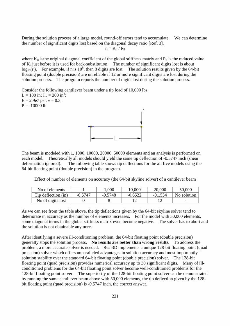
221

During the solution process of a large model, round-off errors tend to accumulate. We can determine the number of significant digits lost based on the diagonal decay ratio [Ref. 3].

ri = Kii / Pii

where Kii is the original diagonal coefficient of the global stiffness matrix and Pii is the reduced value of Kii just before it is used for back-substitution. The number of significant digits lost is about log10(ri). For example, if ri is 108, then 8 digits are lost. The solution results given by the 64-bit floating point (double precision) are unreliable if 12 or more significant digits are lost during the solution process. The program reports the number of digits lost during the solution process. Consider the following cantilever beam under a tip load of 10,000 lbs: L = 100 in; Izz = 200 in4; E = 2.9e7 psi; ν = 0.3; P = -10000 lb

The beam is modeled with 1, 1000, 10000, 20000, 50000 elements and an analysis is performed on each model. Theoretically all models should yield the same tip deflection of -0.5747 inch (shear deformation ignored). The following table shows tip deflections for the all five models using the 64-bit floating point (double precision) in the program.

Effect of number of elements on accuracy (the 64-bit skyline solver) of a cantilever beam

No of elements 1 1,000 10,000 20,000 50,000 Tip deflection (in) -0.5747 -0.5748 -0.6522 -0.1534 No solution No of digits lost 0 8 12 12 -

As we can see from the table above, the tip deflections given by the 64-bit skyline solver tend to deteriorate in accuracy as the number of elements increases. For the model with 50,000 elements, some diagonal terms in the global stiffness matrix even become negative. The solver has to abort and the solution is not obtainable anymore. After identifying a severe ill-conditioning problem, the 64-bit floating point (double precision) generally stops the solution process. No results are better than wrong results. To address the problem, a more accurate solver is needed. Real3D implements a unique 128-bit floating point (quad precision) solver which offers unparalleled advantages in solution accuracy and most importantly solution stability over the standard 64-bit floating point (double precision) solver. The 128-bit floating point (quad precision) provides numerical accuracy up to 30 significant digits. Many of ill-conditioned problems for the 64-bit floating point solver become well-conditioned problems for the 128-bit floating point solver. The superiority of the 128-bit floating point solver can be demonstrated by running the same cantilever beam above with 50,000 elements, the tip deflection given by the 128-bit floating point (quad precision) is -0.5747 inch, the correct answer.

222

A more practical application of the 128-bit floating point (quad precision) may be in the modeling of a rigid diaphragm (e.g. floor with much larger in-plane stiffness than out-of-plane stiffness). Most of the other programs model this kind of rigid diaphragm action through master-slave constraints in order to avoid numerical difficulties. With the 128-bit floating point solver available in Real3D, you may model the floor as a flexible diaphragm, yielding much more realistic results. It should be pointed out that the 128-bit floating point (quad precision) requires twice as much memory as the 64-bit floating point (double precision). It is also significantly slower. However, in situations where the standard 64-bit floating point solver produces unreliable or even wrong results, the 128-bit floating point (quad precision) provides an invaluable alternative. Between faster but wrong results and slower but correct results, you as a responsible engineer probably should choose the latter.

223

Chapter 19: Frequency Analysis The frequency analysis solves for frequencies and corresponding mode shapes (eigenvectors) of the structural system. Many concepts discussed in the previous chapter-“Static Analysis”, apply to the frequency analysis as well.

Solution Algorithm Mathematically, the frequency analysis involves solving the following Eigen problem:

[K] [Φi] = λi [M] [Φi] where [K] is the global stiffness matrix, [M] is the global mass matrix, [Φi] is the ith mode shape and λi is the ith eigenvalues which is equal to the free vibration circular frequency squared (ωi)

2. Other

related values are frequency fi which is 2π ωi and period Ti which is 1 / fi. For practical reasons, we are generally interested only in the lowest eigenvalues (and therefore lowest frequencies). The solution of eigenvalue problems must be iterative in nature because it is equivalent to finding the roots of the polynomial p(λ). The solution algorithm to solve the equation above is given by K.J. Bathe [Ref. 1]. It uses the subspace iteration method to iteratively find the lowest p eigenvalues λ1, λ2,

… λp and corresponding vectors [Φ1], [Φ2], …[Φp]. Eigenvalues are extracted in ascending order. Each eigenvector is then normalized such that [Φi]

T[M] [Φi] = [I] where [I] is the identity matrix, a diagonal matrix with unit values along the main diagonal. A tolerance may be set before the solution to control the convergence of eigenvalues during each successive solver iteration. It is expressed as the following:

tolerancek

i

ki

ki ≤−

+

+

)1(

)()1(

λλλ

(i = 1, 2, …number of requested modes)

where k is the subspace iteration counter. To prevent excessive computing time, a maximum number of subspace iterations may be set before the solution. If the solver reaches this limit without convergence, the eigen results should not be trusted. At the completion of the solution, an error measure is computed for each eigenvalue according to the following [Ref 1]:

Error Measure = )()(

)(1

)()(

2)(

ki

Tki

ki

qq

λ−

Where )(k

iq is the vector in the matrix )(kQ corresponding to

)(kiλ and the eigenvalues are accurate to

about 2s digits if Error Measure is less than 10-2s.

Mass and Stiffness The global mass matrix [M] is diagonal and is computed based on the load combination for frequency analysis and/or additional nodal masses/mass moments of inertia. The load combination for frequency analysis may be specified in Run | Frequency Analysis. The program will automatically

224

convert all forces (not moments) in the positive or negative gravity direction to nodal masses and apply them in all available mass degrees of freedom. Additional nodal masses and mass moments of inertia may be input from Loads | Additional Masses or Input | Additional Masses. Zero terms in the global mass matrix [M] are allowed. The number of eigenvalues requested must be fewer than the mass DOFs which is the number of nonzero diagonal terms in [M]. Due to the lumped mass modeling, the elements should be properly divided or sub-meshed for a continuous vibration model. For example, a beam with uniformly distributed mass should be divided into at least eight elements in order to find accurate vibration results. The load combination for frequency analysis is also used to compute the global stiffness matrix [K] if the model response is not linear. This may be the case if 1). The load combination for frequency analysis is of P-Delta type; or 2). The model contains nonlinear elements such as compression-only springs. In the first case (geometric nonlinearity), the compressive forces decrease the model stiffness (and therefore lengthen the vibration periods of the model) while tensile forces increase the model stiffness. The influence of the axial loads is greater on the lower frequencies than on the higher ones. The effect of nonlinearity on the stiffness matrix of the structure is incorporated as follows:

• An iterative (nonlinear) static analysis is first performed with the loads in the load combination for frequency analysis.

• The stiffness matrix at the end of the static analysis will be used in the frequency analysis. The stiffness therefore includes geometric and element nonlinearities corresponding to the end of the nonlinear static analysis.

Forced displacements at supports are ignored in frequency analysis.

Solution Convergence Due to the iterative nature in the eigen solution, much more computational effort is required (in order to achieve satisfactory convergence) in frequency analysis than in static analysis. Another important difference is solution stability, which is more difficult to achieve in frequency analysis. To ensure that the smallest required eigenvalues and the corresponding eigenvectors have been computed, the program performs a Sturm sequence check after the subspace iterations [Ref 1]. A warning message is given in the solver dialog box if some eigen values are missing after the Sturm sequence check. Under some rare circumstances, the solution may become unstable and the solver has to abort the solution process Several remedies can be used to address the solution instability and solution divergence. 1). Solve for fewer number of modes. 2). Use larger number of iteration vectors. 3). Use 128-bit floating point arithmetics instead of 64-bit floating point arithmetics. These remedies may be used in tandem. Once again, the 128-bit floating point arithematics is especially effective for solution stability. The maximum number of subspace iterations is set to 18 by default. If no convergence is achieved at this limit, you should rerun the frequency analysis with a larger maximum number of subspace iterations.

225

Chapter 19A: Response Spectrum Analysis

Solution Algorithm The response spectrum analysis is done separately in global X, Y and/or Z directions. The following algorithm [Ref. 23] is used in the program. Given the following for mode n Eigen value ωn , eigen vector [Φn], mass matrix [M] and stiffness matrix [K] Generalized load for mode n £n = [Φn]

T[M][ G] where [G] is a vector of influence coefficients of which component i represents a unit acceleration at displacement coordinate i in X, Y or Z direction.

Generalized mass for mode n

=*nM [Φn]

T[M] [Φn]

Effective mass for mode n

=

*n

2

en M

£M n

Participation factor for mode n

∑=

M

M f en

Modal displacement for mode n

Φ=

2*n

n

M

£][}{

n

pann

Sv

ϖ

where Spa is spectral acceleration

Inertia forces for mode n

}]{[}{ nn vKF =

Inertia forces in each global direction are then converted to nodal loads in inertia load cases such as INERTIA_LOADCASE_X_MODE_1, INERTIA_LOADCASE_X_MODE_2 etc. Existing loads in these load cases will be deleted prior to the load conversion. In addition, response spectrum load combinations INERTIA_LOADCOMB_X_MODE_1, INERTIA_LOADCOMB_X_MODE_2 etc. will be created or recreated. Static analysis will be performed on spectrum load combinations (as well as normal user-defined load combinations) automatically.

Modal Combination Modal combinations are calculated in each global direction for results such as displacements, forces and stresses etc. using CQC (complete quadratic combination), SRSS (Square root of sum of squares) and ABSSUM (absolute sum) on the response spectrum load combinations. CQC method for modal

226

combination is applicable to a wider class of structures and is therefore recommended method. When critical damping ratio is 0, CQC method is the same as SRSS method. For more information about these modal combination methods, please refer to [Ref. 14, 23 ]. Normally, modal combination results are all positive due to the sign lost during SRSS, CQC and ABSSUM procedures. However, you can choose to use signage for modal combination results based on the dominant mode (with maximum participation factor) in each global direction.

Directional Combination Modal combination results (Rx, Ry and Rz) is done in each of global directions X, Y and Z. Using directional factors, these directional modal results will be combined into final modal combination results, which will be added to any user-defined load combination results if response spectrum load factor is specified in the load combination definition (see Loads | Load Combinations). Rfinal = Rx * directional_factor_x + Ry * directional_factor_y + Rz * directional_factor_z. An example would be to apply 100% of inertia forces in one horizontal direction plus 30% of inertia forces in the perpendicular horizontal direction. In this case, directional_factor_x = 1.0, directional_factor_z = 0.3 and directional_factor_y = 0. For more information, please refer to Chapter 12 in [Ref. 24].

227

Chapter 20: Concrete Design – ACI 318-02/05/08/11/ 14 The concrete design module performs concrete design for beams, columns and plates (bending only) according ACI 318-02, 05, 08,11 and 14 [Ref. 19]. Static analysis must be performed successfully before concrete design can be performed. Sound engineering judgment is especially important to interpret and apply the design results given by the program. Note: The provisions that apply for ACI 318-02 and 05 shall apply to ACI 318-08, 11 and 14 unless explicitly stated otherwise.

Concrete Column Design General The concrete column module designs concrete rectangular or circular columns against axial, uniaxial or biaxial bending as well as shear based on ACI 318-02/05/08/11/14 Code Provisions. The program generates EXACT (not approximate or empirical) P-Mx-My interaction surfaces for all sections according to user-specified design criteria. The unity check ratio is computed for each column based on capacity interaction surfaces and axial force-biaxial bending in each load combination. Slenderness effects are considered for both non-sway (braced) and sway (unbraced) frames. Shear design in columns is based on the shear force envelope with the option to include or exclude axial force influence on concrete shear capacity. Axial Load and Moment Convention For concrete design, compressive and tensile axial loads have positive and negative signs respectively. The major moment is designated as Mx in design as opposed to Mz used in analysis output. The minor moment is designated as My in both analysis and design. Solution Assumptions

• The strain in reinforcement and concrete is directly proportional to the distance from the neutral axis (ACI 318-02/05 10.2.2).

• The maximum usable strain at the extreme concrete compression fiber is equal to 0.003 (ACI 318-02/05 10.2.3).

• The stress of steel is fs = Es * εs but fs <= fy where Es = 29000 ksi, εs is steel strain and fy is the yield strength of steel (ACI 318-02/05 10.2.4).

• The tensile strength of the concrete is neglected in flexural calculation (ACI 318-02/05 10.2.5). • A uniformly distributed stress of 0.85fc is assumed over an equivalent compression zone

bounded by the edge of the cross section and a line parallel to the neutral axis at a distance a = β1* c where c is the distance from extreme compression fiber to neutral axis (ACI 318-02/05 10.2.7.1).

• β1 = 0.85 – 0.05 * (f’ c - 4) and 0.65 <= β1 <= 0.85 and f’ c unit is ksi • Reinforcement ratio ρ should be 1% <= ρ <= 8% for column sections (ACI 318-02/05

10.2.7.3).

228

Solution Algorithms 1. All sections are EXACTLY solved biaxially based on the solution assumptions above. Each section is solved based on the following steps. 2. Nominal Strength Calculation (Pn, Mnx, Mny) 2a. The nominal capacity of a section is computed at successive choices of biaxial angles. The choices of angles are based on the user input for biaxial angle steps found in the command Concrete Design | Design Options. Biaxial angle steps affect the solution accuracy and speed. For biaxial problems, steps must be multiples of 4. A value of 16 ~ 32 is sufficiently accurate for most sections. The adequacy of biaxial angle steps can be determined by smoothness of the Mx-My interaction diagram. For uniaxial problems, biaxial angle steps should be set to 4. This will give P-Mx (+) at 0 degree angle, P-Mx (-) at 180 degrees angle, P-My (+) at 90 degree angle, P-My (-) at 270 degrees angle. The number of biaxial angle steps is analogous to the number of sides of a polygon used to approximate a circle or ellipse. A uniaxial solution in the program is therefore analogous to using a square to approximate a circle or a rectangle to approximate an ellipse. A biaxial solution with 16 angle steps is analogous to using a 16-sided polygon to approximate a circle or an ellipse. Obviously, the 16-sided polygon is closer or more accurate to approximate a circle than a square. The moral of this comparison is that a low value of biaxial angle steps tends to give more conservative biaxial capacity for the section.

2b). For each biaxial angle, Pn, Mnx, Mny and maximum tensile steel strain εt are computed at successive choices of neutral axis distance c using strain compatibility and stress-strain relations to establish bar forces and the concrete compressive results. The choices of c are based on the neutral axial steps found in the command Concrete Design | Design Options. Neutral axial steps affect the solution accuracy and speed. A value of 250 ~ 500 for neutral axis steps is sufficiently accurate for most sections. The adequacy of neutral axis steps can be determined by smoothness of the P-Mx and/or P-My interaction diagrams. In addition, the program always computes several control points. They are maximum Pn (compression), minimum Pn (tension), fs =0; 0.25fy; 0.5fy and 1.0fy (balanced condition). Concrete displaced by steel may be optionally included or excluded (by default). 2c). Mnx-Mny contour curves are computed for successive choices of axial forces. This is achieved through interpolation on the Pn, Mnx and Mny already calculated for each biaxial angle in the procedure

229

above. The choices of axial forces are based on the neutral axial steps found in the command Concrete Design | Design Options. 3. Design Strength Calculation (φPn, φMnx, φMny) Design strength according to ACI 318-02/05/08/11/14 is obtained by multiplying Pn, Mnx and Mny of each biaxial angle by applying strength reduction factor φ as determined in the following (ACI 318-02/05 9.3.2): Φc = 0.65, α = 0.80 for tied confinement Φc = 0.70, α = 0.85 for spiral confinement for ACI 318-02/05 Φc = 0.75, α = 0.85 for spiral confinement for ACI 318-08/11/14 For (εt <= εy, compression-controlled sections)

φ = Φc For (εt > 0.005, tension-controlled sections)

φ = 0.90 For (εy < εt < 0.005)

φ = Φc + (0.9 - Φc) * (εt - εy ) / (0.005 – εy) where εt is maximum tensile steel strain for the biaxial angle and εy is steel yield strain (at balanced condition) In addition, φ Pn must be always less than the following (ACI 318-02/05 10.3.6.1) Φc * α * [ 0.85 * fc

’ * (Ag – As) + fy * A s] if concrete displaced by steel is excluded or Φc * α * [ 0.85 * fc

’ * Ag + fy * A s] if concrete displaced by steel is not excluded. 4. Unity Check Ratio Unity check ratio is computed for each section based on the loads and the capacity of the section. It is defined as the following: For a given load set (Pu, Mux, Muy), find the section capacity Mx-My contour at φPn= Pu. The unity check ratio for the load set is the larger of:

+

+

)(,

)M( )M(

)(M )M(

max,2

max ny,2

max nx,

2uy

2ux

n

u

P

P

ϕϕϕ

Where (φMnx,max, φMny, max) is the interaction point between the line from point (Mux, Muy) to point (0,

0) and the Mx-My contour line. max,nPϕ is the maximum compression or tension capacity of the section, depending on the positive or negative sign of Pu. If Pu is outside the maximum compression or tension capacity, a unity check ratio of 99.9 is assigned. A unity check ratio equal or less than 1.0 means the design strength is greater than the required strength; and the section is adequate to resist all input loads. A unity check ratio greater than 1.0 means the design strength is less than the required strength and the section is inadequate to resist all input loads. It is important to realize that unity check ratio defined in the program is just a measure of section adequacy against loads. It should not be related to the factor of safety. Unity Check Ratio Calculation Example To illustrate the calculation of unity check ratio in the program, see the following example.

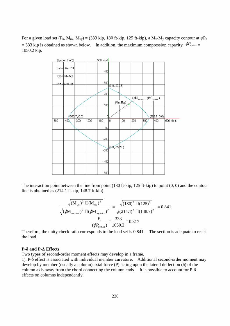
230

For a given load set (Pu, Mux, Muy) = (333 kip, 180 ft-kip, 125 ft-kip), a Mx-My capacity contour at φPn

= 333 kip is obtained as shown below. In addition, the maximum compression capacity max,nPϕ = 1050.2 kip.

The interaction point between the line from point (180 ft-kip, 125 ft-kip) to point (0, 0) and the contour line is obtained as (214.1 ft-kip, 148.7 ft-kip)

841.0 )(148.7 )214.1(

)(125 )(180

)M( )M(

)(M )M(

22

22

2max ny,

2maxnx,

2uy

2ux =

+

+=

+

+

ϕϕ

317.02.1050

333

)( max,

==n

u

P

P

ϕ

Therefore, the unity check ratio corresponds to the load set is 0.841. The section is adequate to resist the load.

P-δ and P-Δ Effects Two types of second-order moment effects may develop in a frame. 1). P-δ effect is associated with individual member curvature. Additional second-order moment may develop by member (usually a column) axial force (P) acting upon the lateral deflection (δ) of the column axis away from the chord connecting the column ends. It is possible to account for P-δ effects on columns independently.

231

2). P-Δ effect is associated with the lateral drifts of the frame members. Additional second-order moment may develop by axial force (P) acting upon the lateral translation (Δ) of the frame nodes relative to their original position. It is NOT possible to account for P-Δ effects on columns independently.

Slenderness Effects For a non-sway frame, P-Δ effect may be safely ignored and the first-order structural analysis is therefore sufficient. The program then accounts for P-δ effect by magnifying the first-order moments using ACI moment magnification method. For a sway frame, the second-order structural analysis must be performed to account for P-Δ effect. In addition, the program accounts for P-δ effect by magnifying the second-order moments using ACI moment magnification method. In fact, all columns in sway frames must first be considered as braced columns under gravity loads acting alone. Braced or Unbraced Column The column is considered braced if one of the following two criteria is met: Criterion 1: Increase in column end moment due to second-order effects is less than 5% of the first-order moment Criterion 2: Stability index Q for the column story under consideration from the first-order analysis

05.0)( 0 <∆∑

=cu

u

lV

PQ (ACI 318-02/05 Eq10-6)

Section Properties for Structural Analysis and Computing K It is important to point out that in both first- and second-order analyses; appropriate member stiffness must be used to account for the effects of axial loads, cracking, and creep.

cc fE 57000= for normal weight concrete

ccc fwE 335.1= for wc between 90 and 155 lb/ft3

Moment of inertia (ACI 318-02/05 10.11.1) = 0.35 Ig for beams and cracked walls = 0.70 Ig for columns and uncracked walls = 0.25 Ig for flat plates and flat slabs Area A = 1.0 Ag

Note: a). Ig and Ag are based on the gross concrete cross section, neglecting reinforcement. a). Ig for Tee beams can be closely approximated as 2 times Ig for the web. b). 0.70 Ig should be used for walls first. If the factored moments and shears indicate that a portion of the wall will crack due to stresses reaching the concrete modulus of rupture, the analysis should be repeated with 0.35 Ig for the cracked portions of the wall. [Ref. 16 pp577] The program allows a user to modify the moments of inertia through Element Cracking Factor from Concrete Design | Cracking Factors. In order to use stiffness reduction, you also need to check “Use

232

cracked section properties (Icr) for members and finite elements” in Analysis Options. This allows you to consider or ignore cracking in the analysis without re-entering element cracking information. Radius of Gyration

gg AIr /= Effective Length Factor K Find relative stiffness ratios ( 21 ΨΨ and ) of columns and beams at the top and bottom joints of the column

∑

∑=Ψ

membersbeamforL

EI

memberscolumnforL

EI

Section properties are the same as used in the first-order analysis (step 1) For practical reasons, 2.0=Ψ for fixed end and 20=Ψ for hinged end. The effective length factor K is solved from the from the following equations For braced frames:

01)2

tan(/

2]

)/tan(

/1[

2421

2

221 =−+−Ψ+Ψ+ΨΨ

KKK

K

K

πππ

ππ

For unbraced frames:

0)/tan(

/

)(6

36)/(

21

221 =−

Ψ+Ψ−ΨΨ

K

KK

πππ

The program provides a tool to calculate the effective length factor K based on the input 21 ΨΨ and . The equations above provide a more accurate K calculation than what is given by (ACI 318-02/05 10.12.1) Unsupported Length Lu The unsupported lengths Luy, Luz of a column are the clear distances between lateral supports in column local y and z directions (ACI 318-02/05 10.11.3.1). A zero value of Lu means that it is equal to the member length between the end nodes. For non-sway frames, an optional check is made kLu / r <= 34 – 12(M1/M2) (ACI 318-02/05 Eq10-7). Braced frame k is used here. Lu is unbraced length in local x and y directions. M1 and M2 are the smaller and larger factored end moments on the compression member respectively. (M1/M2) is positive if the member is bent in single curvature and negative otherwise. For sway frames, an optional check is made kLu / r <= 22 (ACI 318-02/05 10.13.2). Sway frame k is used here. Minimum Moments The program calculates minimum moments for both braced and unbraced frames,

233

)03.06.0(; hPM unmi += , where h is in inches (ACI 318-02/05 10.12.3.2). The program conservatively applies the minimum eccentricity about both axes simultaneously. Equivalent Moment Factor Cm (ACI 318-02/05 10.12.3.1)

0.1=mC if M1 = 0 or M2 = 0 0.1=mC if transverse load existed

4.04.06.02

1 ≥+=M

MCm if end moments only. (ACI 318-02/05 Eq10-13). Although not required,

the program also conservatively applies 4.0≥mC for ACI 318-08/11/14.

The sign of 2

1

M

Mis: positive if the column is bent in single curvature, negative otherwise.

Note, Cm is only applicable to non-sway frames. You have the conservative option to always use Cm = 1.0 from Model Design Criteria under Concrete Design | Design Criteria. Section Properties for Critical Loads Computation The EI used in the frame analysis above is an average value. In designing individual columns, the following reduced EI should be used to reflect the greater chance of cracking:

d

gcIEEI

β+=

1

4.0(ACI 318-02/05 Eq10-12)

The Infamous dβ The ratio of maximum factored axial sustained load to maximum factored axial total load. The factor

dβ accounts for the effects of creep.

Generally: LoadLiveFactoredLoadDeadFactored

LoadDeadFactoredd +

=β

Critical Load Pc

2

2

)( uc kl

EIP

π= where 0.1≤k (ACI 318-02/05 Eq10-10)

Moment Magnification Factor

0.1

75.01

≥−

=

c

u

mns

P

PCδ

(ACI 318-02/05 Eq10-9)

Pu is the average of axial force at both ends. If 075.0

1 <−c

u

P

P, the design fails and a unity check

ratio of 999.9 is assigned.

Other Requirements Reinforcement ratio for columns: Bar requirements: minimum 4 bars for tied columns, 6 bars for spiral columns.

234

Tie requirements: >= #3 for No. 10 longitudinal bars and smaller; >= #4 for No. 11 14, 18 longitudinal bars. Column Trial Size

The ACI code requires that the reinforcement ratio for columns be within 08.001.0 ≤≤ tρ . It is

usually economical to have 02.0~01.0=tρ . For tied columns

( )tyc

us ff

PA

ρ+≥

'40.0

For spiral columns

( )tyc

us ff

PA

ρ+≥

'45.0

Based on rectangular or circular sections used for analysis, the program will generate column sections with different reinforcement configurations.

235

Column Shear Reinforcement The column shear design is based on

usc VVV ≥+ )(φ (ACI 318-02/05 Eq11-1) where 75.0=φ . Given bw, d, fc, fy, number of stirrup legs n, and stirrup (tie) area Av, the required stirrup spacing is computed at every analysis station. Concrete shear strength 1. For Pu < 0 (column subjected to tension)

0500

12 ' ≥

+= dbf

A

NV wc

g

uc φφ (ACI 318-02/05 Eq11-8)

2. For Pu >= 0 (column subjected to compression)

dbfA

NV wc

g

uc

'

200012

+= φφ (ACI 318-02/05 Eq11-4)

Note:

• For circular section, Rbw 2= and d = 0.8(2R) where R is the radius of the circular section. (ACI 318 11.3.3 and 11.5.7.3)

• Nu = 0 if the influence of compression on concrete shear strength is ignored.

• psifc 100' ≤ (ACI 318 11.1.2)

• 60' ≤cf ksi in design of shear reinforcement. (ACI 318-02/05 11.5.2) • Light-weight concrete is not considered. • Torsional forces are not considered.

The following is the algorithm used to compute the stirrup (tie) spacing(s) in the program.

If dbfVV wccu'8φφ >− , the design fails (ACI 318-02/05 11.5.7.9).

If 2

cu

VV

φ< , no stirrup required (ACI 318-02/05 11.5.6.1). The program does not check member

depths when applying minimum shear reinforcement for ACI 318-08/11.

If dbfVV wccu'4φφ ≤− , smax <= min(d/2, 24 in) (ACI 318-02/05 11.5.5.1)

If dbfVV wccu'4φφ >− , smax <= min(d/4, 12 in) (ACI 318-02/05 11.5.5.3)

If 2

cuc

VVV

φφ << , s = min

w

yv

wc

yv

b

fA

bf

fA

50,

75.0 ' <= smax (ACI 318-02/05 11.5.6.3)

Otherwise, s = cu

yv

VV

dfA

φφ

− <= smax (ACI 318-02/05 Eq11-15)

According to ACI 318-02/05, column confinement spacing shall not exceed 16 longitudinal bar diameters, 48 tie bar or wire diameters, or the least dimension of the compression members.

236

The following additional requirements are needed for column spirals:

• The maximum center-to-center spacing:

s < ]1/[45.0

2

−cgcc

ysp

AAfD

fdπ (Derived from ACI 318-02/05 Eq10-5)

• The clear spacing between successive turns shall not exceed 3 inches, nor be less than 1 inch. (ACI 318-02/05 7.10.4.3)

237

Concrete Beam Design General The concrete beam module designs concrete rectangular or Tee beams against enveloped bending about strong axis (local z) and enveloped shear along local y. Axial force, bending about weak axis (local y), and torsion are not considered. Furthermore, no deep beam action is considered. If axial force or biaxial bending actions cannot be neglected, the use of column design module is recommended. Beam Flexural Reinforcement The beam top and bottom flexural reinforcement is computed at each analysis station along the beam length. Minimum reinforcement is computed for the bottom steel. The program designs each beam against positive or negative moment with single layer of tension steel with tension-controlled condition. For flexural design, the critical section at a support may be taken at the face of the support (but not greater than 0.175 * span length from the support center). The program offers an option to account for these conditions by automatically computing beam support widths from Model Design Criteria under Concrete Design | Design Criteria. The following algorithm assumes one layer of tension steel, that is, dt = d, the depth of the tension steel centroid. This assumption is made due to its simplicity and conservative nature and is reasonable unless the tension steel strain is very close to 0.005 – the tension-controlled limit strain. The design result is reflected in top and bottom reinforcement diagrams. Rectangular Beam Flexural Design Algorithm Given b, d = dt, d’, fc, fy and Mu find required As (and As’ if needed) Step 1: Determine maximum moment without compression steel, using the tension-controlled

limit 005.0=tε and 9.0=φ dc 375.00 =

010 ca β=

01'

0 85.0 bafC cf =

)2

( 000

adCM fn −= φφ

yfs fCA /00 =

Step 2: If 0nu MM φ≤ , design the section as singly-reinforced as follows:

)( 2bd

MR u

n φ=

)200

,3

max(85.0

211

85.0 '

min'

'

yy

c

c

n

y

c

ff

f

f

R

f

f=≥

−−= ρρ (ACI 318-02/05 10.5.1)

238

'85.0 c

y

f

dfa

ρ=

1βa

c =

003.0

−=

c

cdtsε

bdAs ρ=

Step 3: If 0nu MM φ> , design the section as doubly-reinforced as follows (still assuming the tension-

controlled limit 005.0=tε and 9.0=φ ):

yss fEc

df ≤

−= )(003.0

'1

0

'

−−

=φ

φ)'('

0'

ddf

MMA

s

nus

)('

'0

y

ssss f

fAAA +=

Note, the tensile steel required to balance the compressive steel is )('

'

y

ss f

fA

The design fails if fs’ < 0. For practical reasons, the design also fails if 0'

2

1ss AA > .

Tee Beam Flexural Design Algorithm Given b, bw, hf , d = dt, fc, fy and Mu, find required As

Step a). Assuming a <= hf and tension-controlled section with 9.0=φ

)( 2bd

MR u

n φ=

−−=

'

'

85.0

211

85.0

c

n

y

c

f

R

f

fρ

)200

,3

max('

minyy

c

ff

f=ρ

),max( min dbbdA ws ρρ=

bf

fAa

c

ys

'85.0=

If a > hf, go to Step b)

1βa

c =

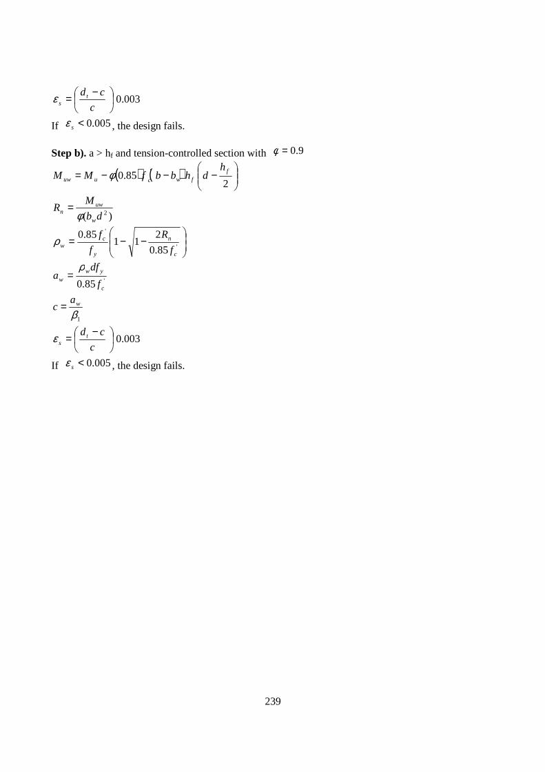
239

003.0

−=

c

cdtsε

If 005.0<sε , the design fails. Step b). a > hf and tension-controlled section with 9.0=φ

( ) ( )

−−−=

285.0 ' f

fwcuuw

hdhbbfMM φ

)( 2db

MR

w

uwn φ

=

−−=

'

'

85.0

211

85.0

c

n

y

cw f

R

f

fρ

'85.0 c

yww f

dfa

ρ=

1βwa

c =

003.0

−=

c

cdtsε

If 005.0<sε , the design fails.

240

Beam Shear Reinforcement The member shear reinforcement (stirrup spacing) is computed at each analysis station along the member length. Stirrup size and number of legs are assumed uniform along the length of a member as part of input. For shear design, sections located less than a distance d from the face of the support may be permitted to be designed for Vu computed at a distance d from the support(ACI 318-02/05 11.1.3.1). The program offers an option to account for these conditions by automatically computing beam support widths from Model Design Criteria under Concrete Design | Design Criteria. The design result is reflected in a stirrup spacing diagram. Beam Shear Design Algorithm The shear design for concrete beam is the same as that of concrete column except the axial force is always treated as zero.

241

Concrete Slab/Wall Design General The concrete slab/wall module designs concrete slabs or walls against enveloped positive and negative Wood-Armer bending moments in slab local x and y directions. Axial force action is ignored. The program produces contours of required areas of steel which can be averaged with some commonsense to finish the design. Wood-Armer Moments Wood-Armer Formula [Ref 18, pp198] is the most popular approach to convert Mx, My and Mxy to orthogonal plate design moments Mux and Muy The procedure to obtain Mux and Muy for designing plate bottom reinforcement is as follows:

• Mux = Mxx + |Mxy| Muy = Myy + |Mxy|

• If Mux < 0 and Muy < 0 Mux = 0

Muy = 0 If Mux < 0 and Muy > 0 Mux = 0

Muy = Myy + |Mxy * Mxy / Mxx| If Mux > 0 and Muy < 0 Muy = 0

Mux = Mxx + |Mxy * Mxy / Myy| • Mux >= 0

Muy >= 0 The procedure to obtain Mux and Muy for designing plate top reinforcement is as follows:

• Mux = Mxx - |Mxy| Muy = Myy - |Mxy|

• If Mux > 0 and Muy > 0 Mux = 0

Muy = 0 If Mux > 0 and Muy < 0 Mux = 0

Muy = Myy - |Mxy * Mxy / Mxx| If Mux < 0 and Muy > 0 Muy = 0

Mux = Mxx - |Mxy * Mxy / Myy| • Mux <= 0

Muy <= 0 Wood-Armer Formula is a lower bound solution method which satisfies the following conditions for a given external load:

• The equilibrium conditions are satisfied at all points in the plate. • The yield strength of the plate elements is not exceeded anywhere in the plate. • The boundary conditions are complied with.

242

A lower bound solution is conservative in nature. Stress Singularity The stresses and bending moments at the point of a concentrated load on the slab are theoretically infinite. This theoretically means that if we used all the steel in the world, we still did not have enough steel to resist the stress at that point. This is of course ridiculous. The reason is of course because we prescribe an impossible loading (“concentrated load”). If we distribute the load over a small area (circle), the stresses become finite. In finite element analysis, the program will never give you a stress of infinite magnitude. Still, at a point of concentrated force such as a column acting on a flat plate, stresses may have rather significant spikes. According to Ugural [Ref 15, pp116], the actual stress caused by a load on a very small area of radius rc can be obtained by replacing the actual rc with an equivalent radius re.

ttrr ce 675.06.1 22 −+= (rc < 0.5t)

ce rr = (rc >= 0.5t) where t is the plate thickness.

By excluding the finite elements (usually finely meshed) near the concentrated loading points, we can provide practical and reasonable design results.

Flexural Reinforcement The plate top and bottom flexural reinforcement in local x and y direction is computed at each nodal point as well as the center. No minimum reinforcement is considered. The program only designs each plate with tension-controlled condition. The procedure is similar to that of concrete beams except no double reinforcement is considered.

243

Chapter 21: Steel Design – AISC 14 th Edition LRFD The steel design module performs steel design for beams and columns according AISC 14th edition LRFD [Ref. 21]. Static analysis must be performed successfully before steel design can be performed. Sound engineering judgment is especially important to interpret and apply the design results given by the program. Due to the fact that the software provides step-by-step calculation procedures, the technical treatment of the design process is kept minimal here.

Section Orientation The orientations of section local X and Y axes of various AISC shapes are shown below (Figure 21.1).

Figure 21.1

244

Member Internal Forces and Moments

1. Axial force P acts perpendicular to the section. Moments Mx and My act about section local X and Y axes respectively. They have the following sign conventions.

Axial Force P: positive for compression; negative for tension Moment Mx: Positive when section top most fiber is under compression. Moment My: Positive when section rightmost fiber is under compression.

Figure 2.1

2. All moments are referenced about the geometric centroid of the gross section. 3. Loads are the required strength computed by the code-specified factored load combinations using either hands or analysis program such as Real3D. It is assumed that an overall 2nd order P-Delta (P-∆) analysis has been performed on a sway structure. If desired, the program uses moment magnification procedure to calculate the P-delta (P-δ) effect, which accounts for slenderness of columns in non-sway structure or for slenderness along the lengths of columns in sway structure. 4. Critical ratio (also called unity check ratio) is computed for each section based on the magnified factored loads and the capacity of the section. Critical ratio equal or less than 1.0 means the design strength is greater than the required strength and the section is adequate. Critical ratio greater than 1.0 means the design strength is less than the required strength and the section is inadequate.

245

Solution Algorithms Because detailed step-by-step calculation procedure is available for each member on Steel Design | Design Result, we will not list the algorithm here.

246

References

1. K.J. Bathe, “Finite Element Procedures” Prentice-Hall, Inc., 1996 2. O.C. Zinenkiewicz, “The Finite Element Method”, 3rd ed., McGraw-Hill Book Company

(UK) Limited, 1983 3. R.C. Cook & D.S. Malkus & M.E. Plesha, “Concepts and Applications of Finite Element

Analysis”, 3rd ed., John Wiley & Sons, Inc., 1989 4. R.H. Macneal & R.L. Harder, “A proposed Standard Set of Problems to Test Finite Element

Accuracy”, pp3-20 of “Finite Elements in Analysis and Design”, North-Holland, 1985 5. J.P. Hartog, “Advanced Strength of Materials”, McGraw-Hill Book Company, 1952. 6. R.J. Roark & W.C. Young, “Formulas for Stress and Strain”, 5th ed., McGraw-Hill Book

Company, 1975. 7. W. McGuire & R.H. Gallagher & R.D. Ziemian, “Matrix Structural Analysis”, 2nd ed., John

Wiley & Sons, Inc., 2000 8. J.S. Przemieniecki, “Theory of Matrix Structural Analysis”, McGraw-Hill, 1968 9. D. Breyer, “Design of Wood Structures”, 3rd ed, McGraw-Hill, 1993 10. J. MaCormac, “Structural Steel Design LRFD Method”, 2nd ed, HarperCollins College

Publishers, 1995 11. A. Tamboli, “Steel Design Handbook LRFD Method”, McGraw-Hill, 1997 12. ACI, “Building Code Requirements for Reinforced Concrete (ACI 318-89) (Revised 1992)”,

American Concrete Institute, Detroit, Michigan. 13. K. Leet & D. Bernal, “Reinforced Concrete Design”, 3rd ed, McGraw-Hill Book Company,

1997. 14. A. K. Chopra, “Dynamic of Structures – Theory and Applications to Earthquake

Engineering”, 2nd ed, Prentice-Hall, 2001 15. Ansel Ugural, “Stresses in Plates and Shells” 2nd Edition, The GcGraw-Hill Companies, Inc.,

1999 16. James G. MacGregor & James K. Wight, “Reinforced Concrete – Mechanics and Design” 4th

Edition, Pearson Prentice Hall, 2005 17. “Notes on ACI 318-02 Building Code Requirements for Structural Concrete”, 8th Edition,

Portland Cement Association, 2002 18. R. Park and W.L. Gamble “Reinforced Concrete Slabs”, John Wiley & Sons, 1980 19. ACI, “Building Code Requirements for Structural Concrete (ACI 318-05) and Commentary

(ACI 318R-05)”, American Concrete Institute, Detroit, Michigan, 2004 20. Arthur H. Nilson, David Darwin, Charles W. Dolan, “Design of Concrete Structures”, 13th

Edition, McGraw-Hill Higher Education, 2004 21. AISC “Steel Construction Manual”, 14th Edition 22. Charles Salmon, John Johnson and Faris Malhas, “Steel Structures” 5th Edition, Pearson

Prentice Hall, 2009 23. James C. Anderson, “Dynamic Response of Structures”, chapter 4 of “THE SEISMIC

DESIGN HANDBOOK” by Springer Science+Business Media New York 24. “Minimum Design Loads for Buildings and Other Structures”, 2006, ASCE.

The following works are not referenced directly in this documentation, but are the primary programming references in the development of this program. Like the great engineering works cited above, these great programming works deserve the respect of being listed here.

247

a. B. Stroustrup, “The C++ Programming Language” 3rd ed., Addison-Wesley Publishing Company, 1997

b. R.Wright & M.Sweet, “OpenGL SuperBible”, 2nd ed., Waite Group Press, 2000 c. D.J. Kruglinski, “Inside Visual C++”, Microsoft Press, 1996 d. M. Woo & J. Neider & T. Davis & D. Shreiner, “OpenGL Programming Guide”, Addison-

Wesley Publishing Company, 1999 e. C. Petzold, “Programming Windows 95”, Microsoft Press, 1996 f. C. Musciano & B. Kennedy, “HTML The Definitive Guide” 3rd ed., O’Reilly & Associates,

Inc., 1998

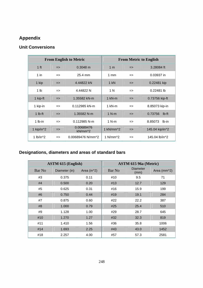
248

Appendix

Unit Conversions

From English to Metric From Metric to English

1 ft => 0.3048 m 1 m => 3.28084 ft

1 in => 25.4 mm 1 mm => 0.03937 in

1 kip => 4.44822 kN 1 kN => 0.22481 kip

1 lb => 4.44822 N 1 N => 0.22481 lb

1 kip-ft => 1.35582 kN-m 1 kN-m => 0.73756 kip-ft

1 kip-in => 0.112985 kN-m 1 kN-m => 8.85073 kip-in

1 lb-ft => 1.35582 N-m 1 N-m => 0.73756 lb-ft

1 lb-in => 0.112985 N-m 1 N-m => 8.85073 lb-in

1 kip/in^2 => 0.00689476 kN/mm^2

1 kN/mm^2 => 145.04 kip/in^2

1 lb/in^2 => 0.00689476 N/mm^2 1 N/mm^2 => 145.04 lb/in^2

Designations, diameters and areas of standard bars

ASTM 615 (English) ASTM 615 96a (Metric)

Bar No Diameter (in) Area (in^2) Bar No Diameter (mm) Area (mm^2)

#3 0.375 0.11 #10 9.5 71

#4 0.500 0.20 #13 12.7 129

#5 0.625 0.31 #16 15.9 199

#6 0.750 0.44 #19 19.1 284

#7 0.875 0.60 #22 22.2 387

#8 1.000 0.79 #25 25.4 510

#9 1.128 1.00 #29 28.7 645

#10 1.270 1.27 #32 32.3 819

#11 1.410 1.56 #36 35.8 1006

#14 1.693 2.25 #43 43.0 1452

#18 2.257 4.00 #57 57.3 2581

249

Index

1

128-bit Solver · iii

2

2D Frame · 80, 123, 124, 200

2D Plane Stress · 124

2D Plate · 124, 195, 211

2D Truss · 80, 124, 195, 200

3

3D Brick · 124

3D Frame · 80, 123, 124, 195, 200

3D Truss · 80, 124, 200

3-Point · 40, 79, 80

6

64-bit Solver · iii

A

Accuracy · 1, 220, 246

Activation · 8, 11, 41, 42, 81

Additional Masses · 11, 12, 97, 119, 121, 122, 126, 224

AISC Table · 65

Analysis Options · 1, 12, 84, 112, 123, 126, 150, 195, 199, 201,

202, 207, 210, 212, 232

Animation · 10, 60, 184

Annotations · 2, 10, 18, 55, 68, 69, 70, 190, 213

Append · 7, 18, 19

Area load · 1, 11, 12, 91, 115, 203, 204

Arithmetic · 220

Assign · 8, 11, 14, 62, 63, 66, 147, 149

Assign menu · 99

B

Batch · 7, 21

Bathe · 209, 219, 223, 246

Beam End Forces & Moment · 132

Beam Segmental Results · 132

Beams · 106, 125

Bending Formulation · 125, 210

biaxial angle · 146, 156, 157, 228, 229

Boundary · 51, 62, 82, 125, 209, 241

Braced · 231, 232

Brick · iii, 10, 12, 13, 69, 70, 135, 143, 194, 215

Brick8 Stresses · 135

Brick8s · 107

C

Cantilever · 221

Capacity ratio · 229

Cartesian · 3, 190

Case-Copy Loads · 11, 96

Circular Shell4s · 10, 75

Clear Results · 8, 42

Clear Undo & Redo · 8, 41, 42

Clipboard · 105, 186

Close File · 18

Closed-Form · 209

Colors · 183

Compatible · 1, 125, 184, 209, 215

Compression · 8, 11, 41, 81, 201

Compression-Only · 83, 109, 126, 197, 206, 211, 217, 224

Concentrated Loads · 11, 12, 90, 113, 203

Concrete Design · 88, 227, 246

Consistent English Units · 180

Consistent Metric Units · 180

constraint · 84, 85, 86, 197

Constraint · 86, 131, 141, 197

Continuous Beam · 1, 10, 71, 199, 205

Contour · 10, 14, 58, 61, 160, 212

Contour Legend · 10, 61

Convergence · 124, 125, 127, 223, 224

Coordinate System · 3, 39, 41, 67, 68, 69, 79, 81, 89, 90, 91, 92,

94, 113, 114, 115, 116, 120, 125, 134, 190, 191, 192, 193,

194, 196, 199, 200, 201, 202, 204, 210, 211, 213, 215, 217

Cross Select · 2

D

Deflection Diagram · 10, 57, 58

Degree of Freedom (DOF) · 195

Dependent · iii

Diagonal Decay · 221

Diaphragm · 1, 11, 12, 84, 85, 86, 111, 112, 125, 126, 182, 202,

222

Directional Combination · 226

Display Modes · 58

Distance List · iii, 31, 32, 33, 35, 67, 71, 73, 74, 76

Distance Tolerance · 181

Drawing Grid · 10, 60, 66, 67

Drift · 11, 12, 86, 121

Drift Node · 11, 12, 86, 121

DXF (import & export) · 2, 7, 19, 20, 21, 22

Dynamic Analysis · 126, 127, 223, 225

250

E

Effective Length Factor · 232

Element Local Angle · 8, 11, 39, 40, 41, 79, 80, 81, 190, 201,

202

Element Merging · 1, 39, 181

Enforced Displacements · 82, 108, 196, 197, 217

Epsilon · 105, 181

Equal Displacement · 85

Equivalent Moment Factor · 233

Error Measure · 138, 223

Euler-Bernoulli · 210

Explode · 8, 37, 181

Export · 7, 20, 21

F

File Backup · 184

File menu · 7, 17, 24, 27

Fixity Flag · 108

Flip Selection · 9, 53

Fluid Load · 11, 94

Freeze Selected · 9, 53, 54

Frequency · 1, 12, 97, 119, 126, 223, 227, 243

Frequency Analysis · 12, 97, 119, 126, 127, 223, 225

G

General Information · 7, 23

Generate Arc Beams · 75

Generate Frames · 10, 71, 73

Generate Non-Prismatic Beams · 76

Generate Shells · 10, 74, 75

Geometric Stiffness · 200

Global Axes · 10, 60, 61

Global Coordinate System · 3, 89, 90, 91, 92, 94, 113, 120, 190,

191, 194, 196, 204, 215, 217

Global Stiffness Matrix · 195, 217, 218, 219, 220, 221, 223, 224

Graphical User Interface · 2

Graphics Scales · 180, 183

Grid · 10, 60, 66, 67, 77

H

Half Band Width · 195, 196

I

Ill-Conditioning · 220, 221

Image Capture · 7, 23

Import · 7, 19, 20

Inclined · 84

Incompatible · 1, 125, 209, 210, 215

In-Plane · 58, 84, 111, 125, 133, 202, 209, 210, 211, 212, 213,

220, 222

Input Data | Springs · 109, 110

Insertion Point · 19, 67, 74, 75

Internal Forces and Moments · 207, 212, 213, 217

Isometric · 8, 43

Isoparametric · 125, 209, 210, 215

Iteration Vectors · 127, 224

Iterations · 124, 127, 217, 223, 224

K

Kirchhoff (thin plate) · 1, 125, 209, 211

L

Line Loads · 11, 12, 91, 114, 203

Line Springs · 12, 110, 206

Linear · 1, 11, 41, 76, 81, 83, 109, 124, 126, 127, 197, 201, 206,

211, 217, 219, 224

Load Case · 11, 12, 87, 217

Load Cases · 87

Load Combination · 11, 12, 87, 88, 113, 217

Load Combinations · 87, 88

Load Diagram · 10, 54

Local Angle · 8, 11, 39, 64, 73, 79, 106, 190, 191, 192, 193

Local Coordinate System · 39, 41, 68, 69, 79, 81, 94, 125, 134,

190, 191, 192, 193, 194, 199, 200, 201, 202, 210, 211, 213,

215, 217

Lock Model · 7, 28

Log File · 17, 27, 126

M

Mass Matrix · 223

Masses · 11, 12, 97, 119, 121, 122, 127, 224

Mat Foundation · 124, 209, 211

Materials · 62, 145, 147, 148, 149, 165

Maximum Nonlinear Iterations · 217

MDI (Multiple Document Interface) · 17, 18

Membrane · 1, 58, 59, 124, 125, 209, 212, 213

Mindlin · 209

MITC4 (thick plate) · 1, 125, 209, 211

Modal · 13, 128, 140, 141, 142, 143, 225, 226

Mode Shape · 10, 59, 60

Model Generations · 1, 10, 11, 68, 70, 71, 73, 74, 75, 76, 77,

79, 88, 94, 95, 199, 209

Model View · iii, 22

Modulation · 59

Moment Inertia · 63

Moment Magnification Factor · 233

Moment releases · iii, 1, 11, 28, 29, 39, 62, 80, 111, 124, 191,

199, 201

Moment Releases · 80, 111

Move · 30

Moving Load · 11, 95, 206

251

N

Named Selections · 44, 55

Named Views · 8, 43

New File · 17

New Window · 15, 57, 58, 59, 60, 188

Nodal Displacements · 13, 129

Nodal Loads · 11, 12, 89, 113

Nodal Resultants · 13, 134, 213

Nodal Springs · 12, 109, 110

Node · 68

Node Numbers · 195

Nodes · 70, 105

Nominal Strength · 228

Non-linear · 124, 217

Nonlinearity · 41, 81, 201, 217, 224

Non-Prismatic Beam · 1, 10, 76, 199

Numerical · 105, 111, 125, 202, 210, 211, 215, 220, 221, 222

O

Open File · 17

OpenGL · ii, 1, 5, 184, 247

Orphaned Node · iii, 8, 9, 39, 50

Out-of-Plane · 211

P

Panning · 1, 9, 18, 28, 43, 45, 46, 188

Parent · iii

Pattern Load · 11, 94, 95

P-Delta & P-delta · 1, 88, 124, 126, 199, 201, 217, 218, 219,

224

Plate & Shell · 9, 14, 50, 52, 123, 124, 149, 150, 153, 159, 160,

161, 192, 195, 200, 210, 211

Point Loads · 11, 12, 90, 113, 203

Poisson Ratio · 62

Precisions · 15, 180, 183

Preferences · 15, 24, 28, 60, 184, 185

Principal Forces & Moments · 13, 133, 153, 154, 155, 159, 160

Principal Stresses · 13, 134, 135

Print · 2, 7, 14, 22, 23, 62, 63, 66, 87, 88, 105, 147, 149, 157

Properties · 105

Q

Quadrilateral · 75, 115, 209, 210

R

Real time · 1

Real Time Motion · 46, 47

Redo · 7, 8, 28, 41, 42

Regular Section · 62, 64

Render · 10, 37, 56, 57, 190

Re-Number · 8, 37, 38

Report View · iii, 22, 23

Reports · 2, 17, 123, 180, 184, 221

Response Spectrum · 12, 97, 121, 127, 225

Restore model · 43

Restraint · 82, 83, 197, 206, 211

Reverse Element Nodes’ Order · 8, 39, 190, 215

Reverse Select · 47

Rigid Diaphragm · 1, 84, 111, 112, 125, 126, 202, 222

Rigid Link · 8, 11, 41, 81

roller · 82, 84, 197

Rotating · 1, 7, 9, 30, 46, 47, 105

Rotational DOFs · 109, 195, 200

Round-off Errors · 220, 221

S

Save File · 18

Save Results · 182

Scale · 31

Sections · 63, 124

Segmental Output · 124

Select All · 9, 48, 52

Select by IDs · 9, 47, 48, 52

Select by Properties · 9, 44, 48, 49, 50, 51, 52

Selection Methods · 2, 47

Self Weight · 8, 11, 41, 93, 94

Self Weight Multiplier · 93, 202, 211, 216

Self Weights · 11, 12, 93, 94, 95, 119, 203, 216

Shear and Moment Diagram · 57

Shear Area · 63, 124, 199

Shear Deformation · 124, 125, 199, 200, 209, 210, 221

Shear Modulus · 62

Shear Wall · 124, 209, 213

Shell4 · 69

Shell4 Forces & Moments · 13, 132, 133

Shell4s · 106, 125

Slenderness Effects · 231

Solid Element (brick) · 1, 10, 44, 58, 69, 73, 107, 125, 135, 190,

194, 215

Solution Accuracy · 146, 220, 221, 228

Solution Algorithm · 219, 223, 224

Splitting Beams · 35, 219

Spreadsheet · 1, 4, 13, 61, 105, 106, 107, 108, 109, 111, 112,

113, 114, 115, 116, 117, 118, 146, 151, 152, 153, 156, 157,

168, 169, 181, 184

Spring · 1, 11, 12, 13, 55, 58, 82, 109, 110, 130, 131, 190, 196,

197, 198, 206, 207, 211

Spring Reactions · 13, 130, 131

Springs · 82, 83

Stability · 220, 231

Static Analysis · 12, 126, 217, 223

Statistics · 7, 27

Steel Design · 243

Stiffness Matrix · 124, 127, 182, 195, 200, 201, 210, 211, 215,

217, 218, 219, 220, 221, 223, 224

Story · 13, 129

Story Drift · 13, 129

Stress Averaging · 125

Stress Stiffening · 199, 200

252

Stresses · 13, 133, 134, 135, 181, 216, 246

Structural Commands · iii, 28

Sturm Check · 224

Sub-Mesh · 36, 75

Subspace Iterations · 127, 223, 224

Support Reactions · 13, 130, 131

Supports · 82, 108

Surface Loads · 11, 12, 92, 93, 116, 117, 118

Switch Coordinates · 8, 38

T

Technical Issues · 189

Temperature · 62

Tension · 8, 11, 41, 81, 201

Tension-Only · 83, 126, 197, 206, 211, 217

Thermal · 93, 117, 118, 206, 211, 216

Thick Plate · 125, 209, 210, 211

Thickness · 65

Thin Plate · 75, 125, 209, 210, 211

Timoshenko · 210

Torsion · 207

U

Unbraced · 148, 167, 231

Undo · 1, 7, 8, 28, 42, 181, 203

Uniform Loads · 11, 12, 91, 114, 115, 203, 204, 205

Unit Cases · 88

Units · 15, 145, 147, 148, 149, 150, 153, 163, 164, 165, 168,

170, 179, 180, 183

Unity Check · 10, 60

Unselect All · 9, 48, 52

Unstable · 39, 127, 220, 224

V

Views · 1, 2, 8, 18, 22, 23, 145, 180, 183, 188

Von Mises Stresses · 59, 134, 135, 213, 216

W

Window/Point Select · 9, 47

Windows · 15, 17, 18, 57, 58, 59, 60, 188

Winkler · 211

Wood-Armer · 14, 159, 160, 241

Z

Zienkiewicz · 209

Zoom Extent · 44

Zoom In · 45

Zoom Object · 44

Zoom Out · 45

Zoom Previous · 44, 45

Zooming · 1, 8, 9, 18, 28, 43, 44, 45, 47, 48, 188

*************************************************** ***************************