a strategy for the management of energy losses in a local
TRANSCRIPT

A strategy for the management of energy losses in a local electricity distribution network
by
Johannes Wilhelmus Fourie
Submitted in partial fulfillment of the requirements for the degree
Master of Engineering (Electrical Engineering)
in the
Faculty of Engineering, the Built Environment and Information Technology
UNIVERSITY OF PRETORIA
October 2004
UUnniivveerrssiittyy ooff PPrreettoorriiaa eettdd –– FFoouurriiee,, JJ WW ((22000055))

Electrical, Electronic and Computer Engineering
i
SUMMARY
This dissertation contains a strategy to minimize the non-technical electrical energy losses
in an electrical distribution network. In order to develop the strategy, a model was
constructed that simulates an electrical distribution network and includes different
parameters that calculate the estimated technical losses in the electricity distribution
network. The model was then used as the base to develop the strategy to minimize the
electrical energy losses in an electrical distribution network.
Increasing energy costs and environmentalists actions to protect the natural resources,
force energy supply companies to conserve and reduce energy usage. Therefore the
research focused on the reduction of electrical energy losses in distribution networks. The
loss occurrences are divided into two categories: technical and non-technical losses.
Reducing these losses ensure that the cost of electricity to customers will be reduced and in
turn improve the efficiency of the distribution network.
The model developed to calculate the non-technical losses in an electrical distribution
network was tested at two different networks. Firstly at the University of Pretoria, where
the network segment consisted of different network busses delivering electrical energy.
Secondly results were obtained in a residential network of the Tshwane Metropolitan
Council. In this network there was only one bus but various different time intervals were
used to determine the time interval most suitable for determining the electrical energy
losses in the electrical distribution network.
The model was used primarily to quantify the technical losses as a base point towards
determining the non-technical losses. Using the model one is able to forecast the technical
energy losses of a section in the electricity distribution network and this enabled one to
develop a strategy to minimize the energy losses in the distribution network. The model
will enable municipalities or electricity distribution companies to estimate electrical energy
losses in their electrical supply networks and facilitate the development of strategies to
reduce electrical energy losses.
KEYWORDS
Technical losses, non-technical losses, electrical distribution network.
UUnniivveerrssiittyy ooff PPrreettoorriiaa eettdd –– FFoouurriiee,, JJ WW ((22000055))

Electrical, Electronic and Computer Engineering
ii
OPSOMMING
Die verhandeling ontwikkel ‘n strategie om die nie-tegniese elektriese verliese in ‘n elektriese
verspreidings netwerk te minimiseer. Om die strategie te ontwikkel was ‘n model ontwikkel wat die
elektriese verspreidings netwerk simuleer. Die model sluit ook veranderlikes in wat die tegniese
verliese van die elektriese verspreidings netwerk bereken. Die model word verder gebruik as die
basis waarop die strategie vir die minimiseering van die elektriese verliese gebaseer word.
Die toename in energie koste en omgewingsbewustes se aksies om die natuurlike hulpbronne te
beskerm, forseer energie verskaffende maatskappy om die energie verbruik te spaar en te
verminder. Daarom word navorsing toegespits op die vermindering van elektriese energie verliese
in elektriese verspreidings netwerke. Die energie verliese kan in twee kategorieë verdeel word nl.:
tegniese verliese en nie-tegniese verliese. Die vermindering van die verliese verseker dat die koste
van elektrisiteit na verbruikers verminder word en verseker ook dat die effektiwiteit van die
verspreidings netwerk verbeter.
Die model om die nie-tegniese verliese in ‘n elektriese verspreidings netwerk te bereken was
getoets in twee verskillende netwerke. Eerstens by die Universiteit van Pretoria, waar die netwerk
segment bestaan het uit verskillende netwerk busse, wat elektrisiteit lewe. Tweedens was resulate
verkry van residensiële netwerk van die Tshwane Metropolitaanse Raad wat slegs uit een bus
bestaan het. Verskillende tyds intervalle was gemeet en daarvolgens was die mees geskikte tyds
interval gekies om die elektriese energie verliese in ‘n elektriese verspreidings netwerk te bepaal.
Die model was hoofsaaklik gebruik om die tegniese verliese te kwantifiseer en is as basis gebruik
vir die bepaling van die nie-tegniese verliese. Deur die model te gebruik is dit moontlik om die
tegniese verliese van ‘n gedeelte van die elektriese verspreidings netwerk te voorspel en
hiervolgens kan ‘n stategie ontwikkel word om die energie verliese in die network te minimeer. Die
model sal stadsrade of elektriese verspredings maatskappye in staat stel om energie verliese in
betrokke elektriese verskaffings netwerke te kan voorspel en sal dit moontlik maak om ‘n strategie
te ontwikkel om energie verliese te verminder.
SLEUTELWOORDE
Tegniese verliese, nie-tegniese verliese, elektriese verspreidings network.
UUnniivveerrssiittyy ooff PPrreettoorriiaa eettdd –– FFoouurriiee,, JJ WW ((22000055))

Electrical, Electronic and Computer Engineering
iii
TABLE OF CONTENTS
SUMMARY I
OPSOMMING II
TABLE OF CONTENTS III
CHAPTER 1: INTRODUCTION 1
1.1. PROBLEM STATEMENT 1 1.2. MAIN AND SPECIFIC OBJECTIVES 3 1.3. CONTRIBUTIONS OF THIS STUDY 4 1.4. OVERVIEW OF DISSERTATION 4
CHAPTER 2: OVERVIEW OF LITERATURE 6
2.1 EFFICIENT ELECTRICITY USE 6 2.1.1. Household sector electricity use 7 2.2.2. Impact of electricity usage on the environment 7
2.2. NON-TECHNICAL LOSSES 8 2.3. TECHNICAL LOSSES 9
2.3.1. Types of technical (conductor) losses 10 2.3.1.1 Copper losses 11 2.3.1.2. Dielectric losses 11 2.3.1.3. Induction and radiation losses 12
2.3.2. Secondary factors influencing technical losses 13 2.3.2.1. Circulating current 13 2.3.2.2. Voltage regulation 13 2.3.2.3. Phase balancing 14 2.3.2.4. Power factor 14
2.3.3. Approaches for loss calculation 14 2.3.3.1. Full accuracy method 14 2.3.3.2. Representative load profile method 15
2.3.4. Calculation of technical loss segments 17 2.3.4.1. Energy meter losses 17 2.3.4.2. Customer connection losses 18 2.3.4.3. Low voltage network losses 18 2.3.4.4. Distribution transformer losses 19 2.3.4.5. Medium voltage network losses 20 2.3.4.6. Distribution substation losses 20 2.3.4.7. Sub transmission network losses 21 2.3.4.8. Energy balance for a distribution network 21
2.4. STRATEGIC PLANNING 22 2.4.1. Planning the strategy 22 2.4.2. Project manager reporting 23
2.5. SUMMARY OF LITERATURE 24
CHAPTER 3: DEVELOPMENT OF THE MODEL AND THE FORMULATION OF THE STRATEGY 25
3.1. NEED FOR EFFICIENT USE OF ELECTRICAL ENERGY 25 3.2. GENERAL DESCRIPTION OF THE FUNCTIONS OF THE MODEL 25 3.3. VALUE SYSTEM 25
UUnniivveerrssiittyy ooff PPrreettoorriiaa eettdd –– FFoouurriiee,, JJ WW ((22000055))
Table of Contents
Electrical, Electronic and Computer Engineering
ii
3.4. FUNCTIONAL ANALYSIS 26 3.5. DEVELOPMENT OF THE MODEL 27
3.5.1. Importing the text files 28 3.5.2. Technical loss calculation algorithms 29
3.5.2.1. Network segment loss calculation 33 3.5.2.2. Other network loss calculation 33 3.5.2.3. Energy meter calculation 33 3.5.2.4. Customer connection calculation 34 3.5.2.5. Transformer/bus loss calculation 34
3.5.3. Correlation of segments 35 3.5.4. Statistical calculation of the segments 36
3.5.4.1. P values 36 3.5.4.2. T-test 38 3.5.4.3. F test 38
3.5.5. Problem area identification 39 3.6. APPROACH IN DEVELOPING THE STRATEGY TO MINIMIZE ELECTRICAL ENERGY LOSSES 41
3.6.1. Calculation of technical losses 43 3.6.2. Measured usage 44 3.6.3. Calculation of non-technical losses 45 3.6.4. Identify problem areas 45
3.6.4.1. Paired-t test 45 3.6.4.2. Analysis of variance 47
3.6.5. Solve problem areas 48 3.7. LIMITATIONS OF MODEL 49 3.8. VERIFICATION OF THE MODEL 50
CHAPTER 4: CASE STUDIES OF THE MODEL 52
4.1 VERIFICATION OF DEVELOPED MODEL AT THE UNIVERSITY OF PRETORIA 52 4.2 VERIFICATION OF DEVELOPED MODEL IN GARSFONTEIN/RETRIEVER 72
CHAPTER 5: CONCLUSIONS 84
5.1 INTRODUCTION 84 5.2 CONCLUSION ON THE OBJECTIVES 84 5.3 CONCLUSIONS AT THE MAIN CAMPUS OF THE UNIVERSITY OF PRETORIA 86 5.4 CONCLUSIONS AT THE TSHWANE METROPOLITAN COUNCIL 86 5.5 RECOMMENDATION AND FUTURE WORK 87
5.5.1. Recommendation on the integration of the strategy into energy management programs 87 5.5.2. Future work 88
REFERENCES 89
APPENDIX A: GENERAL MODULE SOURCE CODE 92
APPENDIX B: GENERAL STRATEGY SOURCE CODE 110
APPENDIX C: UNIVERSITY OF PRETORIA DATA FORMAT SOURCE CODE 115
APPENDIX D: GARSFONTEIN/RETRIEVER DATA FORMAT SOURCE CODE 119
UUnniivveerrssiittyy ooff PPrreettoorriiaa eettdd –– FFoouurriiee,, JJ WW ((22000055))

Electrical, Electronic and Computer Engineering 1
CHAPTER 1: INTRODUCTION
1.1. Problem statement
Increasing energy costs and environmentalists actions to protect the natural resources,
force energy supply companies to conserve and reduce energy usage [1]. Many companies
are also forced to research methods to reduce energy consumption during peak demand
periods as a result of higher tariff that are applicable to energy consumed during peak
demand periods. These tariffs differ by as much as five times standard tariff charge outside
peak periods. Thus, an area that has therefore been receiving particular attention is the
question of how to reduce energy losses that occur in electricity supply networks.
According to Davidson et al.[2], the electrical energy losses can be divided into two main
groups:
Technical losses
• losses due to physical aspect, and
Non-technical losses
• unauthorized line tapping or metering bypassing, and
• inadequate or faulty meters and equipment.
Reducing the technical and non-technical losses will ensure that the cost of electricity to
the supplier will be reduced, as less electricity will be used from the power generating
company. The cost of the electricity to the customer will therefore also be less, as they will
not have to pay for the losses in the electricity supply network. Both these reductions will
have a positive influence on the cost of electricity.
According to Krishnaswamy [3] the following can be investigated to determine the
technical losses in a network:
• the effect of circulating current because of the interconnection of electricity supply
networks, the voltage regulation,
• the phase balance, and
• the power factor.
UUnniivveerrssiittyy ooff PPrreettoorriiaa eettdd –– FFoouurriiee,, JJ WW ((22000055))

Chapter 1 Introduction
Electrical, Electronic and Computer Engineering 2
Municipalities use Krishnaswamy’s methods to determine the losses in the different
sections of a distribution network. The approach is an unpractical method as it uses average
losses over the entire distribution network to determine the technical losses.
The approach used in this dissertation identifies the different types of technical losses in a
distribution network and associate the losses with a percentage of the different segments.
Each section in the distribution network is then statistically evaluated to determine if the
energy balance holds for that section of the network. This approach can identify a problem
area should it exist within the network segment of the electrical distribution network. By
identifying problem areas and resolving the problems electrical distribution companies can
improve the energy distribution and save the electrical consumer revenue.
The focus of this dissertation is to develop a strategy that will minimize the non-technical
electrical energy losses of an electricity distribution network. To be able to develop a
strategy, a model that simulates the electricity supply network is constructed and includes
different parameters to calculate the estimated technical losses of the electricity distribution
network. This model is used as the base to develop a strategy to minimize the energy losses
of the electricity distribution network. The strategy was evaluated in a section of the Main
Campus of the University of Pretoria’s electricity distribution network. The strategy was
also verified in a section of the Tshwane Metropolitan Council. Figure 1.1 shows an
electricity distribution network and each box in the setup is a point of measurement.
UUnniivveerrssiittyy ooff PPrreettoorriiaa eettdd –– FFoouurriiee,, JJ WW ((22000055))

Chapter 1 Introduction
Electrical, Electronic and Computer Engineering 3
Figure 1.1: An electricity distribution network
1.2. Main and Specific Objectives
This dissertation formulates a strategy to minimize energy losses in an electrical
distribution network. The strategy focuses primarily on quantifying technical losses as a
base point towards determining the non-technical losses. To determine the technical losses
a model was constructed to quantify these losses and to calculate the non-technical losses
in an electricity distribution network.
The model used enables one to forecast the electrical losses of a section in the electricity
supply network. With the use of this model one is able to develop a strategy to minimize
the electrical losses in an electricity distribution network.
The main objective of this dissertation is to develop a strategy to minimize energy losses in
an electrical distribution network. To achieve the main objective the following specific
objectives were determined:
• construction of a model to determine the technical losses,
Distribution network
Transmission and Generation
33 kV
22 or 11 kV
380 or 220 V Sub – Substation Minisub – Mini substation HH - Household
Sub 1 Sub 2 Sub 3
Mini sub 1
Mini sub 2
HH 2 HH3 HH 1
UUnniivveerrssiittyy ooff PPrreettoorriiaa eettdd –– FFoouurriiee,, JJ WW ((22000055))

Chapter 1 Introduction
Electrical, Electronic and Computer Engineering 4
• determine a method to calculate the non-technical losses,
• determine a procedure to identify the problem areas, and
• construct a matrix to prioritize the problem areas.
1.3. Contributions of this study
This dissertation contributes in developing a strategy to minimize electricity losses in an
electricity distribution network. Quantifying the magnitude of technical and non-technical
losses determines the total electrical energy lost in the electricity distribution network.
According to Chen et. al.[4] the technical losses are specific and can therefore be
calculated. He also points out that minimization of technical losses are minimal in
comparison to the non-technical losses. This dissertation will therefore endeavor to
minimize the non-technical losses and the benefits obtained are:
• a reduction in electrical energy generation and system capacity, and
• a reduction in the cost of electrical energy to the consumer.
1.4. Overview of dissertation
This dissertation constructs a model to forecast the electrical energy losses in an electricity
distribution network. The model incorporates the factors and parameters that contribute to
the electricity losses in a section of the electricity distribution network. It is able to
quantify the technical and non-technical losses in the electricity distribution network and
the model was used to develop a strategy to minimize energy losses in the network. This
enables electricity distribution companies in South Africa to estimate electricity losses in
their electricity distribution networks.
In chapter 2 an overview is giving to show the different mathematical equations that can be
used to determine the electrical energy losses in the distribution network. This chapter also
explains the relative work already done in the determination of the electrical energy losses
in an electrical distribution network. In chapter 3 the development of the model was
explained in detail with the derivation of the strategy of the minimization of the electrical
energy losses in the distribution network. Chapter 4 discusses the case studies and the
UUnniivveerrssiittyy ooff PPrreettoorriiaa eettdd –– FFoouurriiee,, JJ WW ((22000055))

Chapter 1 Introduction
Electrical, Electronic and Computer Engineering 5
results of the case studies that have been done. The first part of the chapter discusses the
results obtain using different busses in the distribution network and the second part
discusses the results of different time interval and the effect that the periods have on the
results. In Chapter 5 a conclusion of the work was drawn as well as recommendations for
future work.
UUnniivveerrssiittyy ooff PPrreettoorriiaa eettdd –– FFoouurriiee,, JJ WW ((22000055))
Electrical, Electronic and Computer Engineering 6
CHAPTER 2: OVERVIEW OF LITERATURE
2.1 Efficient electricity use
Efficient use of electrical energy includes all the technical and economical (non-technical)
measures aimed at reducing the electrical energy demand of an electricity distribution
network. Although implementation of an electrical energy management strategy may
require an initial investment, short-term financial returns can be achieved through lower
cost due to the reduced electrical energy demand. In this dissertation the focus is to
develop a strategy to reduce electrical losses in an electricity distribution network, which
have a high electrical energy demand and thus a high potential for energy savings.
Electrical energy usage is vital to economic development in developing countries and
poverty will not be reduced without greater use of electricity [5]. Assuming that the energy
demand grows by 2.6 % per year, the total energy consumption by the year 2050 would
double that of the level of consumption in 1998 [5]. The challenge is to break the link
between economic growth and electric energy consumption by pursuing efficient
production processes and reducing waste. At the same time, the link between electric
energy consumption and pollution will be broken and the economy will rely more on
renewables and therefore using fossil fuels more efficiently.
Electricity power industries in developing countries according to World Bank lose more
than 20% of their generated electricity to theft or inefficiencies. One way to stop these
losses is to encourage private-sector participation in trying to stop the theft. However,
many projects aimed at stopping theft and cutting electricity losses have not achieved their
goal. Therefore a huge scope exists to reduce electrical energy losses in developing
countries that use district distribution systems. The World Bank has assisted in reducing
the electrical energy losses and has reduced losses remarkably: 15-20 % of the input
electrical energy has been saved by implementing private-sector participation. In South
Africa the government uses demand side management initiatives to reduce electrical
energy. The private-sector company is been rewarded for their participation in an electrical
savings bonus or a penalty if no energy is been saved over a period of time.
UUnniivveerrssiittyy ooff PPrreettoorriiaa eettdd –– FFoouurriiee,, JJ WW ((22000055))

Chapter 2 Overview of literature
Electrical, Electronic and Computer Engineering 7
The electrical usage in the residential sector is inefficient according to the World Bank and
electrical energy savings can be increased either by using energy-saving lighting or more
importantly the electrical consumption for residential users could be investigated and the
demand side management strategic planning done to reduce electrical energy losses in this
sector. In the next section the electricity demands for the distribution networks in South
Africa is discussed as well as the impact that electricity generation has on the environment.
2.1.1. Household sector electricity use
According to Lane et al. [6], residential households electricity demand contribute to 20%
of the national peak electricity demand and is the largest customer base sector in an
electrical energy distribution network. The contribution in electrical energy consumptions
in South Africa is therefore expected to rise to 37% by the year 2015 if customer growth
and electricity demand increases steadily. Thus, the increase in electrical energy demand
forces electrical supply companies to either cut down on electrical energy losses or to
generate more energy that will have a negative impact on the environment.
2.2.2. Impact of electricity usage on the environment
Electricity generation accounts for a huge portion of unwanted emissions into the
atmosphere [6]. The greenhouse gases that are typically produced by power stations are
carbon monoxide (CO), methane (CH4), nitrogen oxides (NOX), nitrous oxide (N2O) and
carbon dioxide (CO2). Making use of effective energy management is a cost effective
alternative to decreasing pollution in the electrical energy industry [6]. Studies show that
power stations in South Africa produce 92,73 kg of greenhouse gasses per GJ (Giga Joule)
of electric energy [8]. According to Davidson et al. [2], Eskom have 10 800 GWh
(Gigawatt hour) of electrical energy losses in a typical month. The impact of the energy
losses on the environment is indicated in Table 2-1. From Table 2-1 it is evident that losses
in an electricity distribution network have an enormous impact on the environment. To
reduce electrical distribution network losses will therefore amount to significant financial
and natural resource savings.
UUnniivveerrssiittyy ooff PPrreettoorriiaa eettdd –– FFoouurriiee,, JJ WW ((22000055))

Chapter 2 Overview of literature
Electrical, Electronic and Computer Engineering 8
Table 2-1.: Environmental impact of electrical energy losses [2] Environmental
measure Typical impact
Impact due to losses
Water use 1.25 kL/MWh 13500 ML Ash emission 0.37 kg/MWh 4 ktonne Coal use 480 kg/MWh 5.18 Mtonne CO2 output 900 kg/MWh 9.72 Mtonne SOX output 7.4 kg/MWh 80 ktonne NOX output 3.7 kg/MWh 40 ktone
To reduce the effect that electrical energy generation has on the environment, the energy
must be efficiently managed. Two major factors that contribute to the loss in electrical
energy are non-technical losses and technical losses.
2.2. Non-technical losses
An ideal electrical energy distribution network will generate electrical power X and
distribute the electrical power to the network equal to X. Due to losses in the transmission
and distribution sections of the electrical energy network less than X electrical energy is
distributed to the network. This loss in electrical energy is the system losses of the
electrical distribution network. It is given by:
∑ ∑ ∑+= lossesSystemdDistributeGenerated PPP (2-1)
The system losses of an electrical distribution network can be divided into two main
groups the technical losses and the non-technical losses. Non-technical losses are dominant
in the lower sections of the electricity distribution network and are losses due to:
• unauthorized line tappings
• meter tampering
• damage to cables and other electrical equipment, and
• inaccurate estimations of non metered or measured supplies (public lighting, municipal
facilities, park facilities, incorrect CT or VT ratios, faulty meters).
A reduction in non-technical losses will have a direct economic benefit in reducing
electricity prices paid by the customer and it will increase the revenue of electrical
UUnniivveerrssiittyy ooff PPrreettoorriiaa eettdd –– FFoouurriiee,, JJ WW ((22000055))

Chapter 2 Overview of literature
Electrical, Electronic and Computer Engineering 9
distribution supply companies as the electrical energy losses decrease and more electrical
energy could be sold to the customer. The non-technical losses are almost impossible to
calculate from first principles as these losses are depended on human intervention on the
electrical energy distribution network. Therefore to calculate the non-technical losses an
indirect approach is needed. The indirect approach to calculate the non-technical losses of
an electrical distribution network is given by Davidson et. al. [2]
( )∑ ∑ ∑+−=− lossesTechnicaldDistributeGeneratedtechnicalNon PPPP (2-2)
The non-technical and technical losses of the distribution network is interconnected and
calculated as the total losses of the electrical distribution network. Therefore it is necessary
to derive calculated estimated values for either the technical or non-technical losses in the
network. As mentioned the non-technical losses are impossible to calculate, thus the
technical losses must be derived and quantified for an electrical distribution network [2].
The next section will discuss the different types of technical losses and methods used to
calculate technical losses in an electrical energy distribution network.
2.3. Technical losses
Technical losses according to Davidson et al. [2] are due to the current flowing in a
conductor generating heat and affecting resistance, causing electricity loss. In all
conductors at least one of the following losses occurs:
• copper losses
• dielectric losses, and
• induction/radiation losses.
These conductor losses are also called technical losses, thus it includes line losses in the
distribution network and the conduction losses of transformers. The main factors impacting
technical losses according to Neetling et al. [8] are:
• substations,
• circuits,
UUnniivveerrssiittyy ooff PPrreettoorriiaa eettdd –– FFoouurriiee,, JJ WW ((22000055))

Chapter 2 Overview of literature
Electrical, Electronic and Computer Engineering 10
• voltage levels,
• type of circuits (air, underground, mixed, ie. location of cattle),
• type of load (residential, commercial, industrial, mixed),
• transformation points,
• installed capacity,
• predicted demand, and
• length of the circuits.
Technical losses represent 6-8 % of the cost of generated electricity and 25% of the cost to
deliver the electricity to the customer [2]. A reduction in technical losses will originate two
important savings:
• a decrease in energy required to be generated, and
• a decrease in the maximum demand.
The next section will focus on the three types of conductor losses mentioned above namely
copper losses, dielectric losses and induction/radiation losses.
2.3.1. Types of technical (conductor) losses
Atmospheric temperature is the most important parameter influencing the fluctuation in
conductor losses. Therefore, a heat balance equation is considered to calculate conductor
losses of an electrical distribution network. The heat balancing equation states that the heat
absorbed by the conductor is equal to the heat emitted by the conductor. Heat absorbed by
the conductor is due to the resistance of current flowing in the conductor at a specific
temperature and the heating of the sun on the conductor. The heat emitted by the conductor
is due to induction and radiation. An equation of the heat balancing equation is given as:
[10]
InductionRadiationSun PPPRIemittedHeatabsorbedHeat
+=+
=2 (2-3)
UUnniivveerrssiittyy ooff PPrreettoorriiaa eettdd –– FFoouurriiee,, JJ WW ((22000055))

Chapter 2 Overview of literature
Electrical, Electronic and Computer Engineering 11
2.3.1.1 Copper losses
Copper conductor windings are used in electricity distribution networks due to its high
conductivity. The high ductility of the copper makes it effortless to bend the conductors
into tight bends around the magnetic core and thus minimize the amount of copper volume
needed for the windings. At high current densities losses are significant and equal to I2R.
I2R losses are influenced by temperature as follows: [11]
( )( ) mWCtRIRI t /2012022 °−+= α (2-4)
Where α is the temperature coefficient (typically 0.004 /m˚C), R20 is the resistance (Ω) of
the conductor at 20°C, I in amps (A) and t is the temperature in ˚C of the conductor. These
losses are inherent in all conductors because of the finite resistance of the conductors.
Transformer losses in the electricity distribution network are also considered as copper
losses due to the internal impedance of the transformer coils and the core losses.
Transformers connected in the energy distribution network are connected permanently to
the power supply system; therefore the no-load losses of the transformers must be taken
into consideration.
No-load losses according to Sen [12] depend on the maximum value of flux in the core.
The flux or eddy current loss of a transformer is
2
max2 fBKP ee = (2-5)
where Pe is the eddy current loss in the transformer, Ke is a constant value depending on
the type of material and the lamination thickness in mm, B is the flux density (T) and f is
the frequency (Hz) of the transformer.
2.3.1.2. Dielectric losses
Dielectric absorption is remnant polarization trapped on dielectric interfaces [13].
Dielectric absorption cause significant losses in an electricity distribution network due to
UUnniivveerrssiittyy ooff PPrreettoorriiaa eettdd –– FFoouurriiee,, JJ WW ((22000055))

Chapter 2 Overview of literature
Electrical, Electronic and Computer Engineering 12
the heating of the conductors. This heating is primarily due to the sun heating the earth and
is calculated as follow:
dSKP iSSun ⋅⋅= W (2-6)
Where Psun is the heating of the conductor due to the sun in Watt, KS is the solar absorption
coefficient (m), Si is the solar radiation intensity (typically 1300 W/m2), and d is the
diameter of the conductor (m).
2.3.1.3. Induction and radiation losses
Induction and radiation losses are produced by the electromagnetic fields surrounding
conductors. Induction losses occur when magnetic fields around a conductor link to
another magnetic object and current is inducted to the object, thus the power is lost to the
object [2]. In an electrical distribution network induction losses occur due to wind and are
given as:
( ) ( )( ) ( )
δ⋅=<−⋅⋅=
>−⋅⋅⋅=
uVandsmwindspeedformWTTdP
smwindspeedformWTTdVP
acInduction
acInduction
/14.0/9
/14.0/2.1025.175.0
52.0
(2-7)
Where V is the effective wind velocity (m/s), d is the diameter of the conductor (m), Tc is
the temperature of the conductor (typically 53.994 K), Ta is the ambient temperature
(typically 330 K), u is the actual wind velocity (m/s), and d is the relative air pressure.
Radiation losses are the result of magnetic lines of force about a conductor that do not
return when the cycle alternates. The lines of force project into space and are being
absorbed by another object. Radiation losses are calculated using:
( ) mWTTdSKP aCRRadiation /44 −⋅⋅⋅⋅= π (2-8)
UUnniivveerrssiittyy ooff PPrreettoorriiaa eettdd –– FFoouurriiee,, JJ WW ((22000055))

Chapter 2 Overview of literature
Electrical, Electronic and Computer Engineering 13
Where KR is the radiation coefficient, S is the Stephan constant (5.71 × 10⁻⁹ W/m2), d is the
diameter of the conductor (m), Tc is the temperature of the conductor (typically 53.994 K),
and Ta is the ambient temperature (typically 330 K).
2.3.2. Secondary factors influencing technical losses
Although copper losses, dielectric losses and induction and radiation losses are the major
types of losses that occur in an electrical distribution network, secondary types of electrical
energy losses also occur in the network. According to Davidson et al [2] these secondary
losses occur due to circulating currents in the network, voltage regulation equipment,
techniques and equipment used to balances the voltage phases of the network and
equipment to correct the power factor of the network.
2.3.2.1. Circulating current
With highly interconnected electrical distribution networks striving to avoid failures of the
network, circulating currents occur in the electrical distribution network and therefore
increases the losses of the network. Maintaining constant voltage levels in the distribution
network minimize circulating current losses.
2.3.2.2. Voltage regulation
Line losses in an electricity distribution network increases with the square of the load
current when the resistance is constant. Thus by maintaining or decreasing the voltage
across the load would reduce the line losses of the electrical distribution network [2].
UUnniivveerrssiittyy ooff PPrreettoorriiaa eettdd –– FFoouurriiee,, JJ WW ((22000055))

Chapter 2 Overview of literature
Electrical, Electronic and Computer Engineering 14
2.3.2.3. Phase balancing
Phase balancing is of significance when the electrical distribution network becomes
heavily overloaded. According to Krishnaswamy [3] in order to minimize the electrical
power losses in an overloaded network, the phase load maximum deviation must be below
10 %.
2.3.2.4. Power factor
At unity power factor the current is minimum and any reactive component will cause an
increase in current with a resultant increase in the real power loss of the electricity
distribution network. For electricity distribution networks with large inductive loads, losses
due to inductive energy (VArs) become significant.
The secondary factors influencing technical losses are relatively small compared to the
losses in the conductors. Therefore the secondary losses are negligible and omitted in this
dissertation. In the next section approaches to calculate technical losses will be discussed.
2.3.3. Approaches for loss calculation
The calculation of technical losses can be done using various approaches with different
degrees of accuracy. For the management of technical losses a balance between absolute
calculation accuracy and the effort must prevail. According to Nortje [14], acceptable
approaches to calculate technical losses of an electricity distribution network can be
divided into two groups. These are the full accuracy methods and methods of
representative load profiles as discussed below.
2.3.3.1. Full accuracy method
According to Nortje [14], a full accuracy method can only be achieved with an electrical
distribution network model and statistical metering instrumentation installed at each
household receiving electricity. A comprehensive electrical distribution network model
UUnniivveerrssiittyy ooff PPrreettoorriiaa eettdd –– FFoouurriiee,, JJ WW ((22000055))
Chapter 2 Overview of literature
Electrical, Electronic and Computer Engineering 15
includes the flow layout diagram of the electricity through the network, the different
conductor lengths and the resistivity of each conductor. This method is therefore an
impractical method to use for large electrical distribution networks as changes to the
network would alter the parameters of the model and updating of the parameters could be
neglected resulting in an error calculating the technical losses of the electrical distribution
network. A further contributing factor to the impracticality of the method is the enormous
number of measurements, data capturing and manipulation of costs that must be done. The
full accuracy method although impractical for large networks, works well for smaller
electricity distribution networks or in conjunction with other loss calculation methods.
2.3.3.2. Representative load profile method
As with the full accuracy method the representative load profile method also requires a
representative electrical distribution network model for technical loss calculation. The
technical loss calculation methodology also requires the monthly measurement of electrical
household energy (kWh). From the representative electrical model and the electrical
household energy measurement it is possible to use sampled electrical household energy
data averages over a specific time interval to establish an average representative monthly
electrical household load profile as illustrated in Figure 2.1.
UUnniivveerrssiittyy ooff PPrreettoorriiaa eettdd –– FFoouurriiee,, JJ WW ((22000055))

Chapter 2 Overview of literature
Electrical, Electronic and Computer Engineering 16
Typical Load Profile
0
20
40
60
80
100
120
140
0:00
0:40
1:20
2:00
2:40
3:20
4:00
4:40
5:20
6:00
6:40
7:20
8:00
8:40
9:20
10:0
0
10:4
0
11:2
0
12:0
0
12:4
0
13:2
0
14:0
0
14:4
0
15:2
0
16:0
0
16:4
0
17:2
0
18:0
0
18:4
0
19:2
0
20:0
0
20:4
0
21:2
0
22:0
0
22:4
0
23:2
0
Time
Load
Figure 2.1: Typical residential load curve
Thus with the representative profile method an estimated diversity behavior could be
determined empirically for any number of consumers, assuming that the diversity affects
the load factor ie. constant loads and the diversity factor and the load factor relationship is
linear to the diversity factor. The representative load profile method assumes the following:
[15]
∑ ∑ ∑−= SoldEnergyEnergyIncomingLossesEnergy (2-9)
Equation 2-9 is commonly used in municipalities and load supply authorities in South
Africa to estimate the electrical energy used by customers. This assumption calculates the
electrical power losses by adding and subtracting power at specific times in the electricity
distribution network. The advantages using this assumption in conjunction with the
representative load profile method is that it is relatively easy to calculate the power
differences and there are only two input parameters used (incoming power and power sold)
to calculate the power differences. The disadvantage of this approach is that it depends on
the correctness of the estimated load profiles at each segment in the electricity distribution
network. An electricity distribution network consists of different segments that distribute
UUnniivveerrssiittyy ooff PPrreettoorriiaa eettdd –– FFoouurriiee,, JJ WW ((22000055))

Chapter 2 Overview of literature
Electrical, Electronic and Computer Engineering 17
electricity to the customers. The different segments of the network will be discussed in the
next section.
2.3.4. Calculation of technical loss segments
The sectors of an electricity distribution network consist of two main groups, the primary
feeders and the distribution feeders. The combination of the primary feeders and the
distribution feeders of an electrical distribution network account for two thirds of the
electrical energy losses in the network [16]. These results are based on physical
measurements and a practical guideline for electricity distribution companies to determine
technical losses in an electricity distribution network. The hierarchy of an electrical
distribution network consists of a substation, primary lines, service transformers, secondary
stations and electrical services. (Refer to Figure 1.1)
According to Oliveira et al [17] the electrical distribution hierarchy of an electrical
distribution network could be subdivided into eight different segments, namely: energy
meters, customer connections to the network, low voltage networks, distribution
transformers, medium voltage networks, distribution substations, sub transmission systems
and other technical losses as shown in Figure 2.2. Other technical losses include equipment
losses in capacitors, voltage regulators, connectors and insulators. A theoretical method of
evaluation of these different distribution segment losses is discussed below in terms of the
load currents used by the different electricity distribution segments. In determining the load
currents, representative load profiles were obtained that represents the daily usage of the
electricity.
2.3.4.1. Energy meter losses
Technical losses in energy meters are due to iron losses in the voltage coils of the energy
meters and may be assumed as constant in the electricity distribution network, since the
energy meters do not depend on the current flowing in the electricity distribution network.
According to Oliveira et al [17] losses in energy meters (em) in kWh can be obtain by:
UUnniivveerrssiittyy ooff PPrreettoorriiaa eettdd –– FFoouurriiee,, JJ WW ((22000055))

Chapter 2 Overview of literature
Electrical, Electronic and Computer Engineering 18
( )1000
32 321 TiiiNpe mmm
⋅++⋅⋅= (kWh/day) (2-10)
where pm is the average demand losses of each voltage coil of the meter (W), Nm is the
total number of energy meters, i1 is the percentage of single-phase meters, i2 is the
percentage of double-phase meters, i3 is the percentage of three-phase meters, and T is the
time interval considered (hours).
2.3.4.2. Customer connection losses
The computation of losses in customer connections is based on the assumption that the
length and electrical resistance of the conductor was previously defined [14]. The daily
energy losses (er) are given by:
10001
2∑=
⋅∆⋅⋅⋅=
tN
ii
r
ItLRke (kWh/day) (2-11)
where k is the number of conductors connected to the customers and current flow is under
normal conditions (k = 2 for single and double phase and k = 3 for three phase), R is the
conductor electrical resistance (Ω/km), L is the average lateral length (km), Ii is the electric
current on the lateral for time interval t (A), ∆t is the time interval duration (hour), and Nt
is the number of daily intervals. Equation 2-11 is divided by a thousand to express the
value in kilowatt instead of watt. In calculating the customer connections a constant current
is assumed meaning that the current level does not vary with the supplied voltage. Thus the
current can be evaluated as a function of the interval demand and the rated voltage.
2.3.4.3. Low voltage network losses
The representative load profile method, the corresponding currents for each measured
interval t and the representative low voltage distribution network configuration could be
used to evaluate the low voltage network technical losses in all the branches of the
UUnniivveerrssiittyy ooff PPrreettoorriiaa eettdd –– FFoouurriiee,, JJ WW ((22000055))

Chapter 2 Overview of literature
Electrical, Electronic and Computer Engineering 19
network. The network branches as shown in Figure 2-2 represent a three-phase conductor
and a ground conductor.
Figure 2.2: Network branches in a low voltage distribution network [17]
The branch currents results from Kirchhoff's current law applied to each network node to
give the resultant sum of the currents are equal to zero. The daily energy losses for a given
network branch (es) can be evaluated by:
( )∑ ∑= =
∆⋅
⋅=
96
1 1
2,1000
1t
N
itiis tIRe
cond
kW/day (2-12)
Where Ri is the conductor electrical resistance (Ω/km), Ii,t is the electric current i on the
conductor time interval t (A), ∆t is the time interval duration, and Ncond is the number of
conductors (phases and ground) for each branch. Equation 2-12 is divided by a thousand to
express the value in kilowatt [14]. The summation value of 96 is representative of 15
minute intervals for a day.
2.3.4.4. Distribution transformer losses
Electrical distribution network currents are determined for all branches of the network up
to the transformer node. Therefore the currents for phase and ground conductors, for every
interval t, at the distribution transformer result from the representative load profile applied
to the low voltage network. Given the transformer rated data, daily electrical energy losses
for a distribution transformer (et) are given by:
UUnniivveerrssiittyy ooff PPrreettoorriiaa eettdd –– FFoouurriiee,, JJ WW ((22000055))

Chapter 2 Overview of literature
Electrical, Electronic and Computer Engineering 20
∑=
∆⋅
⋅⋅+⋅⋅=
96
1
2
24t N
tNCuNfet t
SSSpSpe kVAh (2-13)
Where SN is the transformer rating (kVA), St is the transformer loading for time interval t
(kVA), pfe is the rated iron losses (per unit (pu)), pcu is the copper losses (pu), and ∆t is the
interval duration (hours). The summation value of 96 is representative of 15 minute
intervals for a day [14].
2.3.4.5. Medium voltage network losses
Computation of losses for a medium voltage electrical distribution network is analogous to
the method used for the low voltage electrical distribution networks but the medium
voltage network use different parameters. The medium voltage distribution network
parameters used are the demand loads of the distribution transformers, the medium voltage
customers demand and public lighting transformers [17].
2.3.4.6. Distribution substation losses
Representative feeder load curves are obtained as a result from the application of the
representative load profile method applied to the medium voltage distribution networks.
The aggregation of a load curve of a substation's outgoing feeders leads to the substation
load curve. Given the rated data of the substation transformers, the corresponding daily
losses of the distribution substation (et) can be determined by: [14]
∑=
∆⋅
⋅⋅+⋅⋅=
96
1
2
24t N
tNCuNfet t
SSSpSpe kVAh/day (2-14)
Where SN is the transformer rating (kVA), St is the transformer loading for interval t
(kVA), pfe is the rated iron losses (pu), pcu is the copper losses (pu), and ∆t is the interval
duration (hours). The summation value of 96 is representative of 15 minute intervals for a
day [17].
UUnniivveerrssiittyy ooff PPrreettoorriiaa eettdd –– FFoouurriiee,, JJ WW ((22000055))
Chapter 2 Overview of literature
Electrical, Electronic and Computer Engineering 21
2.3.4.7. Sub transmission network losses
Losses in the sub transmission network is estimated by the use of a percentage index,
obtained by the application of the representative load profile method to a given segment of
the electrical distribution network. These indexes are regularly recomputed as possible
changes in the distribution network configurations may occur [17].
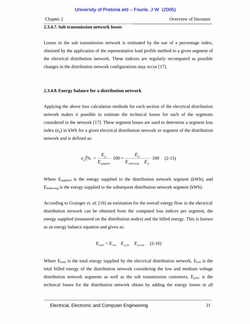
2.3.4.8. Energy balance for a distribution network
Applying the above loss calculation methods for each section of the electrical distribution
network makes it possible to estimate the technical losses for each of the segments
considered in the network [17]. These segment losses are used to determine a segment loss
index (ep) in kWh for a given electrical distribution network or segment of the distribution
network and is defined as:
( ) 100100%supplied
⋅+
=⋅=pfollowing
ppp EE
EE
Ee (2-15)
Where Esupplied is the energy supplied to the distribution network segment (kWh), and
Efollowing is the energy supplied to the subsequent distribution network segment (kWh).
According to Grainger et. al. [16] an estimation for the overall energy flow in the electrical
distribution network can be obtained from the computed loss indices per segment, the
energy supplied (measured on the distribution nodes) and the billed energy. This is known
as an energy balance equation and given as:
comptecpcontotal EEEE ,, ++= (2-16)
Where Etotal is the total energy supplied by the electrical distribution network, Econ is the
total billed energy of the distribution network considering the low and medium voltage
distribution network segments as well as the sub transmission customers, Ep,tec is the
technical losses for the distribution network obtain by adding the energy losses in all
UUnniivveerrssiittyy ooff PPrreettoorriiaa eettdd –– FFoouurriiee,, JJ WW ((22000055))

Chapter 2 Overview of literature
Electrical, Electronic and Computer Engineering 22
segment of the network considered, and Ep,com is the commercial or non-technical losses for
the electricity distribution network.
A estimation for the non-technical losses Ep,com and the corresponding percentage index is
given by:
( ) 100% ,, ⋅=
total
compcomp E
Ee (2-17)
In the next section a strategic plan layout will be discussed in an effort to minimize the
electrical losses of an electrical energy distribution network.
2.4. Strategic planning
Strategic planning is an organization form of project management that is designed to
handle all types of projects ranging from small feasible studies to massive projects [18],
[19]. The most important person involved in the strategic planning process is the project
manager. The project manager’s involvement in the project and the communication to
executives and lower level personnel often make the difference between a well
implemented strategy and one of catastrophe. This section will discuss important
considerations to implement a strategy.
2.4.1. Planning the strategy
Planning a strategy is a function that should be performed by project managers. Project
managers normally use a matrix structure in an effort to obtain the most effective and
efficient utilization of resources while they attempt to achieve the objectives of the project
within the constraints of time, performance and cost. For a project to be within constraints
the goals and objectives of the strategic plan must be clearly identified, together with any
limiting factors haltering the time, cost and performance of the project. Project managers
prefer to work in concrete rather than abstract notation and therefore they must implement
UUnniivveerrssiittyy ooff PPrreettoorriiaa eettdd –– FFoouurriiee,, JJ WW ((22000055))

Chapter 2 Overview of literature
Electrical, Electronic and Computer Engineering 23
the strategic plan they developed themselves. Project managers that plan a strategy should
take the following into consideration:
• Environmental analysis
• Setting objectives
• List alternative strategies
• List possible threats and opportunities
• Prepare forecasts
• Select a strategy portfolio
• Prepare action programs
• Monitor and control the project
2.4.2. Project manager reporting
Strategic planning managers should report high in the organization hierarchy and must
have sufficient authority to obtain qualified resources. Often functional groups are
nearsighted and assign their best resources to those projects that can be expected to yield
immediate profits. This nearsightedness must at all time be avoided as the success of
project management is based on the motivational behavior of the project manager seeing
the project from birth to death. Seeing the result of such a project is probably the strongest
motivational force in any form of project or management of a project.
Strategic management reporting is designed to force conflicts to be resolved at the lower
levels of the project implementation thus freeing the project managers for more vital
concerns. Although this philosophy is acceptable conflicts that arise during the strategic
planning process should be made known to executives rather than trying to solve them at
the lower levels of the project implementation. This should avoid catastrophe to the
implementation and control of the project.
In strategic planning, project managers must realize that, more often than not, articulating
the project strategy to lower level personnel may prove detrimental as this would take
away the projects competitiveness from other companies regarding the same projects.
UUnniivveerrssiittyy ooff PPrreettoorriiaa eettdd –– FFoouurriiee,, JJ WW ((22000055))

Chapter 2 Overview of literature
Electrical, Electronic and Computer Engineering 24
2.5. Summary of literature
The efficient use of electrical energy will slow the destruction of the environments natural
resources and will also reduce the cost of electricity for the consumers. As discussed in the
literature study the technical losses in an electricity distribution network can be calculated.
Thus reduction in electricity generation will be due to non-technical losses and a strategy
to limit the non-technical losses will be derived in the next chapter.
UUnniivveerrssiittyy ooff PPrreettoorriiaa eettdd –– FFoouurriiee,, JJ WW ((22000055))

Electrical, Electronic and Computer Engineering 25
CHAPTER 3: DEVELOPMENT OF THE MODEL AND THE FORMULATION OF
THE STRATEGY
3.1. Need for efficient use of electrical energy
The inefficiency of electrical energy usage is mainly due to losses in the low voltage
segments of an electrical distribution network and is subdivided into technical and non-
technical losses. Technical losses as explain can be calculated and used to estimate the total
losses on the distribution network. Using the estimated technical loss value of a segment of
the network and the value of the total electrical energy delivered to the segment of the
distribution network, the non technical losses can be identified in the distribution network.
The identification of the problems that cause the non technical losses creates opportunities
for improving the efficiency of electrical energy used in an electrical distribution network.
In this chapter the model constructed to calculate the technical losses and the process to
identify the problems causing the non technical losses in the electrical energy distribution
network will be discussed.
3.2. General description of the functions of the model
To determine the technical losses a model was constructed to quantify the technical losses
in an electricity distribution network. The model forecasts the technical losses of a section
in the electricity distribution network and it is used to calculate an estimated value of the
electrical energy used by a section in the distribution network. The method used to
calculate the technical losses of an electrical distribution network provides estimated
energy loss values for each segment in the distribution network.
3.3. Value system
In the dissertation a model is constructed to forecast the electrical energy losses in an
electricity distribution network. This model incorporates the factors and parameters that
UUnniivveerrssiittyy ooff PPrreettoorriiaa eettdd –– FFoouurriiee,, JJ WW ((22000055))

Chapter 3 Development of the model and the derivation of the strategy
Electrical, Electronic and Computer Engineering 26
contribute to electrical energy losses in a section of the electricity distribution network.
Using the factors and parameters it enables the model to quantify the technical losses in the
electricity distribution network. This is used to calculate the non-technical losses in a
section of the distribution network that enables distribution companies to estimate
electricity losses and identify problem areas in their electricity distribution networks.
3.4. Functional analysis
Figure 3-1: Functional diagram of the model
Figure 3-1 displays the functional diagram of the model. The functional units (FU) are
explained as follows:
FU 1 - Method that calculates the technical losses of a section in the electricity
distribution network.
FU 2 - Measuring data received from the meters implemented in a section of the
electricity distribution network.
FU 3 - Determine the total losses and the non-technical losses of the network.
FU 4 - Identify the areas with the highest non-technical losses also referred to as
problem areas.
FU 5 - Solve the problem areas identified in FU 4.
FU 1 Determine
technical losses
FU 2 Measured usage
FU 3 Difference equals non-
technical losses
FU 4 Identify
problem areas
FU 5 Solve problem
areas
UUnniivveerrssiittyy ooff PPrreettoorriiaa eettdd –– FFoouurriiee,, JJ WW ((22000055))

Chapter 3 Development of the model and the derivation of the strategy
Electrical, Electronic and Computer Engineering 27
3.5. Development of the model
The model that will be used to develop a strategy to minimize the electrical energy losses
in an electrical distribution network has five distinct steps. Firstly, the integral part of the
model is the calculation of the technical losses in the distribution network. This is done
using Microsoft Excel calculations and Visual Basic programming language to calculate
each segments technical loss for the entire distribution network. Secondly, the technical
losses in each segment are compared with the measured outgoing electrical energy of the
distribution network segment. This correlation of the technical losses is used to draw
conclusions on the correctness of the distribution of electrical energy in the distribution
network. A flow diagram of the development of the different processes implemented to
develop the model is shown in Figure 3-2.
Figure 3.2: Flow diagram of calculation of technical losses connecting to the model to
determine electrical energy losses.
The model uses electrical measured data from different segments of the distribution
network as input to evaluate losses in the electrical distribution network. All the electrical
data measured at different segments in the distribution network over a period of time (ie.
daily, weekly, monthly) is exported to a tab delimited text file. This is done to standardize
the format of the electrical data. These different exported text files are imported into a
Microsoft Excel spreadsheet to calculate the total electrical energy used in the different
segments of the distribution network and the segment losses of the distribution network is
calculated. From the results obtained in the calculation of the technical losses a correlation
External data (Text files)
Export data to text files
User graphic interface Data imported and calculation done
Data correlation between incoming and
outgoing data
Strategy to identify problem areas
Strategy results to user interface
UUnniivveerrssiittyy ooff PPrreettoorriiaa eettdd –– FFoouurriiee,, JJ WW ((22000055))

Chapter 3 Development of the model and the derivation of the strategy
Electrical, Electronic and Computer Engineering 28
to identifying the problem areas in the distribution network could be determined between
the incoming electrical power of a network segment and the outgoing electrical power of
the segment. The next sections will discuss the methodology used to evaluate the different
results for the model in determining a strategy for the minimization of non-technical losses
in an electrical distribution network.
3.5.1. Importing the text files
The electrical data imported needs to be specified by four parameters in order to identify
the different network segments in the distribution network. The parameters are the name of
the meter, the bus name the electrical energy is sent from, the bus name the electrical
energy is sent to, and the type of network segment the electrical energy is sent from. It is
not necessary to define a parameter for the type of network segment the electrical energy is
sent to because the model assumes that all electrical energy is transported from an energy
bus to another electrical energy bus. With this assumption the model could determine
where the bus is sending the electrical energy. The model further assumes that if no
electrical transformation occurs on the bus in the distribution network the connection of the
network segment to another segment in the distribution network is equal to the customer
connection percentage losses.
The meter names of the electrical distribution network are taken as a base point for
importing the meter reading values into the spreadsheet. This meter reading values logged
could be in any time interval as long as the various logged values of the meter readings are
for the same specified time duration (eg. a month). Thus meter A could be half hourly
measured for a month and meter B could be daily measured for a month. The model will
use these electrical energy measurements and add each meters measured values for the
specific time interval (a month) to evaluate the electrical distribution network segments.
An example of the imported electrical data is shown in Table3-1.
UUnniivveerrssiittyy ooff PPrreettoorriiaa eettdd –– FFoouurriiee,, JJ WW ((22000055))

Chapter 3 Development of the model and the derivation of the strategy
Electrical, Electronic and Computer Engineering 29
Table 3-1 : Importation of electrical energy data (8 November 2003) Time pta1incomer pta2incomer pta3incomer gwtrf1 gwtrf2 erika 01:00 354.0 378.0 348.0 32.0 32.0 28.0 02:00 360.0 384.0 348.0 32.0 32.0 32.0 03:00 360.0 384.0 342.0 32.0 32.0 28.0 04:00 360.0 378.0 348.0 32.0 31.2 32.0 05:00 354.0 378.0 342.0 32.0 32.8 28.0 06:00 360.0 384.0 348.0 32.8 32.8 36.0 07:00 354.0 378.0 342.0 31.2 31.2 32.0 08:00 354.0 378.0 342.0 32.8 32.8 32.0 09:00 354.0 378.0 342.0 32.0 32.0 32.0 10:00 360.0 384.0 348.0 36.8 36.8 36.0 11:00 360.0 378.0 342.0 43.2 44.0 40.0 12:00 348.0 378.0 336.0 40.0 40.8 32.0
The importation of the different network segments measurements are done automatically
and the user of the software must be aware that the meter names, bus name from the
network, the bus name to the network, and the network segment from the network will
influence the electrical distribution network evaluation. Thus if these parameters are
incorrectly defined or misspelled the evaluation of the distribution network will be
incorrect.
3.5.2. Technical loss calculation algorithms
Calculating the technical losses of an electrical distribution network is subdivided into
eight different areas where problems could occur and they are:
• energy meters,
• customer connections to the network,
• low voltage networks,
• distribution transformers,
• medium voltage networks,
• distribution substations,
• sub transmission systems, and
• other technical losses.
UUnniivveerrssiittyy ooff PPrreettoorriiaa eettdd –– FFoouurriiee,, JJ WW ((22000055))

Chapter 3 Development of the model and the derivation of the strategy
Electrical, Electronic and Computer Engineering 30
The identification of these different problem areas were discussed theoretically in the
literature study and showed that it is almost impossible to determine all the different
parameters of a distribution network. In this model a different approach than the theoretical
calculation was used to be able to use a minimum of parameters but still be able to identify
the problem areas in the electrical distribution network. The model uses a percentage
estimation of the loss parameters defined for the different segments in the distribution
network. This approach although not as accurate as the theoretical calculation, gives an
indication of the electrical energy lost in the network segment and are used to determine
the total technical losses of the electrical distribution network. The approach also makes
the implementation of the model practically feasible.
The percentage calculations in the model define a minimum and maximum percentage
parameter for the different network segments in the distribution network. These parameters
are used to calculate the losses of each segment in the electrical distribution network as a
percentage of the input electrical energy to the network segment. Small errors in the
measurements of the meter readings are eliminated in the model as a typical value for the
electrical energy lost in each segment is calculated. This typical energy loss value is the
average value of the minimum and maximum electrical energy loss in each segment of the
electrical distribution network.
There are eight different network problem areas in which electrical energy losses could
occur in the distribution network and the model assumes that electrical energy flow from a
bus onto a cable to another bus in the electrical distribution network. A bus is a point in the
electrical distribution network where one or more electrical connections are connected
together. These assumptions conclude that the electrical losses in the distribution network
could be divided into two main groups. They are the losses on the cables and the losses on
the bus of the distribution network. The losses occurring in the cables of the distribution
network are:
• the sub transmission losses,
• the medium voltage network losses,
• the low voltage network losses,
• customer connection losses,
• energy meter losses,
UUnniivveerrssiittyy ooff PPrreettoorriiaa eettdd –– FFoouurriiee,, JJ WW ((22000055))

Chapter 3 Development of the model and the derivation of the strategy
Electrical, Electronic and Computer Engineering 31
• and other components.
The losses occurring on the bus of a distribution network are:
• the distribution substation losses,
• the distribution transformer losses,
• the customer connection,
• and other components losses.
Take note that customer connection losses and other components losses could occur in both
the cables and the bus of the distribution network.
With the four input parameters obtained from importing the meter measurements as text
files. An algorithm was used to determine the different busses of the distribution network.
The algorithm is used for both the bus from which the electrical energy is flowing and for
the bus to which the electrical energy is flowing. The algorithm’s pseudo-code is given as:
valueadd = false
i = 0
Busname(i) is the names of the bus defined
Busvalue(i) is the electrical energy value of the bus defined
For x = 0 To Number of meters
testname = Get the test bus name
testvalue = Get the value of the electrical energy
For j = 0 To i
If testname = BusNames(j) Then
BusValue(j) = BusValue(j) + testvalue
valueadd = True
End If
Next j
If valueadd = False Then
UUnniivveerrssiittyy ooff PPrreettoorriiaa eettdd –– FFoouurriiee,, JJ WW ((22000055))

Chapter 3 Development of the model and the derivation of the strategy
Electrical, Electronic and Computer Engineering 32
i = i + 1
BusNames(i) = testvalue ;Add a new busname
BusValue(i, 1) = test ;Add a new busvalue
Else
valueadd = False ;Reset the valueadd value
End If
Next x
With this algorithm the different busses from and to a network segment are defined and the
difference of each network segment is determined. This is used to estimate the technical
losses of each network segment and to calculate the total technical losses of the distribution
network.
The algorithm for the determination of the electrical distribution network losses uses the
following steps to determine the losses:
• the loss calculation of the different network segments on the network,
• the calculation of the other losses on the network,
• the calculation of the energy meters on the distribution network,
• the calculation of the customer connection losses on the network segment, and
• the calculation of the transformer/bus losses of the distribution network.
A schematic diagram of the determination of the losses is shown in Figure 3-3.
Figure 3-3 : Steps in determining network segment losses in a electrical distribution network
Electrical distribution network calculation
Network segments
Other losses
Energy meters
Customer connections
Transformer/bus
Subtransmission
Medium voltage
Low voltage
Distribution sub
Distribution transformer
UUnniivveerrssiittyy ooff PPrreettoorriiaa eettdd –– FFoouurriiee,, JJ WW ((22000055))

Chapter 3 Development of the model and the derivation of the strategy
Electrical, Electronic and Computer Engineering 33
3.5.2.1. Network segment loss calculation
As shown in figure 3-3 the calculation of the different network segments is divided into:
• sub transmission losses,
• medium voltage network losses, and
• low voltage network losses.
These different network losses are identified from the “type of network segment from”
input parameter and the associated network segment loss is calculated as a percentage of
the input electrical energy to the particular network segment.
3.5.2.2. Other network loss calculation
The other technical losses are calculated if the type of the network segment states other
losses. This difference could be either due to capacitor banks installed in the network
segment or due to voltage regulators with feedback systems implemented on the network.
The parameter “other technical losses” enables the user to define any unfamiliar or
unknown network design layouts.
3.5.2.3. Energy meter calculation
The calculation of losses occurring in energy meters is done assuming that all the energy
losses of electrical energy meters are approximately the same percentage of electrical
energy used by the network segment. This assumption can be used since the electrical
energy meter losses in an electrical distribution network are small compared to all other
losses influencing the electrical distribution network. The modeling of energy meter losses
defines a meter name for each meter measuring in the distribution network and the energy
meter loss calculation uses the sum of the specific defined meter measurements from the
network to calculate a percentage energy meter loss for each meter.
UUnniivveerrssiittyy ooff PPrreettoorriiaa eettdd –– FFoouurriiee,, JJ WW ((22000055))

Chapter 3 Development of the model and the derivation of the strategy
Electrical, Electronic and Computer Engineering 34
3.5.2.4. Customer connection calculation
There are three possibilities in determining if a segment of the network is connected to the
customer. The first is if the input parameter for the type of network segment is omitted the
model assumes that the network segment is connected to a customer and the loss
calculation is associated with the percentage of the “customer connections” parameter of
the electrical energy in the segment. The second is if the parameter defining the network
segment is omitted the model assumes that the network segment is connected to a customer
and calculates the loss as a percentage of the input energy of the network segment. The
third is if the bus defined by the model is omitted, the model assumes a customer
connection and the loss in the network segment is calculated as a percentage of the input
energy to the bus.
3.5.2.5. Transformer/bus loss calculation
Losses that occur on the bus of an electrical distribution network could be one of the
following: [20]
• distribution transformer losses,
• distribution substation transformer losses, or
• customer connection losses.
The different losses on the bus are determined using the “input” parameter of the bus to
which the electrical energy is flowing. If these electrical energy parameters for the “bus to”
and the “bus from” differ there is a electrical transformation in electrical energy on the
network bus. However, if the "bus name to" and the "bus name from" stays the same there
is no transformation on the network bus and the model assumes the losses on the bus of the
distribution network is the same as the assumption used for a customer connection loss on
the network. There are two different possibilities if the network parameters differ. Firstly
the energy could flow from the transmission network systems to the medium voltage
network of the distribution network and these losses are the distribution sub station losses
and calculated as a percentage of the electrical energy input at the bus. The second
possibility is the medium voltage network that distributes the energy to a low voltage
UUnniivveerrssiittyy ooff PPrreettoorriiaa eettdd –– FFoouurriiee,, JJ WW ((22000055))

Chapter 3 Development of the model and the derivation of the strategy
Electrical, Electronic and Computer Engineering 35
network in the distribution network. These losses in the conversion of the network is
known as the “distribution transformer losses” [20] parameter and calculated as a
percentage of the input energy of the network on the bus.
3.5.3. Correlation of segments
The correlation of values according to the oxford dictionary means the interdependence of
value quantities. In the model the actual measured electrical energy of the different
network segments is related to the estimated electrical energy of the different network
segments. As discussed previously the estimated electrical energy losses could be
determined and from these different calculated electrical energy loss values, typical values
are derived for each of the different segments in the distribution network. As mentioned
previously these typical values are derived due to the fact that the measurements of the
electrical energy in the network may be inaccurate in the model. The model therefore uses
a maximum and minimum tolerance value for this typical network estimation values in an
effort to minimize the effect of small variances in the meter measurements. These
minimum and maximum values are also used to calculate the minimum and maximum
values for the measured values of the different segments of the network. These maximum
and minimum values will not influence the calculation of the determination of the non-
technical losses because the same minimum and maximum percentages are used to
calculate both the estimated and measured values of the network and the values are a
relationship that will increase and decreases as the percentage values increase or decrease.
All the different losses in the network are calculated in the model and for each value a
minimum and maximum values is calculated as a percentage of the specific network loss.
From these calculations the total estimated electrical energy usage for the different busses
are projected. The percentage difference of the projected electrical energy usage of the
different busses and the total measured electrical usage for the busses are calculated with
the projected electrical usage for the busses used as the reference point for each bus.
UUnniivveerrssiittyy ooff PPrreettoorriiaa eettdd –– FFoouurriiee,, JJ WW ((22000055))

Chapter 3 Development of the model and the derivation of the strategy
Electrical, Electronic and Computer Engineering 36
3.5.4. Statistical calculation of the segments
The model uses the following statistical calculations to identify potential problems in the
electrical distribution network:
• the determination of a p value using a two-tailed paired-t test for each bus on the
distribution network,
• calculate the f test value of each of the distribution network busses,
• the standard deviation of each of the busses on the distribution network, and
• calculating the confidence intervals electrical power of the distribution network bus.
3.5.4.1. P values
To understand P values, one needs to understand fixed level testing [21]. With fixed level
testing, a null hypothesis is proposed along with a level for the test, usually 0.05. All
possible outcomes of the experiment are listed in order to identify extreme outcomes that
would occur less than 5% of the time in aggregate if the null hypothesis were true. This set
of values is known as the critical region because if any of the values are observed,
something extreme has occurred. Data is collected and if any one of those extreme
outcomes occurs the results are said to be significant at the 0.05 level. The null hypothesis
is rejected at the 0.05 level of significance. This procedure is known as fixed level testing
because the level of the test is fixed prior to data collection. The procedure begins by
specifying the hypothesis to be tested and the test statistic to be used along with a set of
outcomes that will cause the hypothesis to be rejected. Only then is data collected to see
whether they lead to rejection of the null hypothesis.
Many researchers realized the limitations of reporting on research results when the results
achieve the 0.05 level of significance. The question of whether a result was just barely
significant or wildly so remains unanswered? Would data that was significant at the 0.05
level be significant at the 0.01 level? Even if the results are wildly statistically significant,
is the effect large enough to be of any practical importance?
UUnniivveerrssiittyy ooff PPrreettoorriiaa eettdd –– FFoouurriiee,, JJ WW ((22000055))

Chapter 3 Development of the model and the derivation of the strategy
Electrical, Electronic and Computer Engineering 37
It therefore became common practice to report the observed significance level (or P value),
the smallest fixed level at which the null hypothesis can be rejected. If your personal fixed
level is greater than or equal to the P value, you would reject the null hypothesis. If your
personal fixed level is less than the P value, you would fail to reject the null hypothesis.
For example, if a P value is 0.027, the results are significant for all fixed levels greater than
0.027 (such as 0.05) and not significant for all fixed levels less than 0.027 (such as 0.01). A
person who uses the 0.05 level would reject the null hypothesis while a person who uses
the 0.01 level would fail to reject it.
A P value is often described as the probability of seeing results as more extreme as those
actually observed if the null hypothesis were true. The P value is just another way to
describe the results of fixed level tests. Every so often, a call is made for a ban on
significance tests. The main reason behind these movements is that P values tell us nothing
about the magnitudes of the effects that might lead to the rejection or failure to reject the
null hypothesis. Significance tests blur the distinction between statistical significance and
practical importance. It is possible for a difference of little practical importance to achieve
a high degree of statistical significance. It is also possible for clinically important
differences to be missed because an experiment lacks the power to detect them. However,
significance tests provide a useful summary of the data and these concerns are easily
remedied by supplementing significance tests with the appropriate confidence intervals for
the effects of interest.
When hypotheses of equal population means are tested, determining whether P is less than
0.05 is just another way of examining a confidence interval for the mean difference to see
whether it excludes 0. The hypothesis of equality will be rejected at level α if and only if a
100 (1 - α) % confidence interval for the mean difference fails to contain 0. For example,
the hypothesis of equality of population means will be rejected at the 0.05 level if and only
if a 95% confidence interval for the mean difference does not contain 0. The hypothesis
will be rejected at the 0.01 level if and only if a 99% confidence interval does not contain
zero.
As useful as confidence intervals are, they are not a cure-all. They offer estimates of the
effects they measure, but only in the context in which the data was collected. It would not
UUnniivveerrssiittyy ooff PPrreettoorriiaa eettdd –– FFoouurriiee,, JJ WW ((22000055))

Chapter 3 Development of the model and the derivation of the strategy
Electrical, Electronic and Computer Engineering 38
be surprising to see confidence intervals vary between studies much more than any one
interval would suggest. This can be the result of the technician, measurement technique.
3.5.4.2. T-test
The two-sample paired t test is used to test the null hypothesis of the population mean [22].
Given two paired sets Xi and Yi of n measured values, the paired t-test determines whether
they differ from each other in a significant way under the assumptions that the paired
differences are independent and identically normally distributed.
The criteria used to determine if a paired t-test can be used is that the number of points in
each data set must be the same, and they must be organized in pairs, in which there is a
definite relationship between each pair of data points .
The calculation of the p value returns the two-tailed p value of a paired-t test. The t test
generates a standard score value for each bus value with respect to the minimum, typical
and maximum value of each of the different busses on the network. It returns a p value for
each bus on the distribution using the two-tailed probability for the normal distribution.
This function is used to assess the likelihood that the actual measured electrical energy
output for a specific bus and the estimated electrical energy for the same bus are derived
from the same electrical energy input bus on the distribution network.
3.5.4.3. F test
An F-test is used to test if the standard deviations of two populations are equal [23]. This
test can be a two-tailed test or a one-tailed test. The two-tailed version tests against the
alternative that the standard deviations are not equal. The one-tailed version only tests in
one direction, that is the standard deviation from the first population is either greater than
or less than the second population standard deviation. The choice in this dissertation is the
two-tailed test therefore it tests if the standard deviations are not equal.
UUnniivveerrssiittyy ooff PPrreettoorriiaa eettdd –– FFoouurriiee,, JJ WW ((22000055))

Chapter 3 Development of the model and the derivation of the strategy
Electrical, Electronic and Computer Engineering 39
The f-test use two independent samples of size N1 and N2 to measure for the probability
that they have the same variance. The estimators of the variance are s12 and s2
2 and the test
statistic ratio T = s12/ s2
2, which follows an F Distribution.
More specifically, the p-value of a statistical significance test (f-test) represents the
probability of obtaining values of the test statistic that are equal to or greater in magnitude
than the observed test statistic. To calculate a p-value, sample data are collected from the
different network segments and calculates the appropriate test statistic for the sample [24].
The f test statistical function used in the model returns the two-tailed probability that the
variances in the actual measure electrical energy and the estimated electrical energy are not
significantly different. This function is used to determine whether the measured and
estimated electrical energy have significantly different variances.
The confidence interval in the model calculates the mean of the bus of both the measured
and estimated electrical energy. It is used in the model to determine, with a particular level
of confidence that could be altered in the model, the lowest and highest electrical energy
level of use for a particular bus in the electrical distribution network. This level of
confidence it compared to the actual measured value of the electrical energy used by the
bus and the confidence interval should be an order or more lower than the actual measured
electrical energy to be assumed operating correctly. If the value for the confidence interval
and that of the actual measured values are in the same order the difference between the
measured electrical energy and that of the estimated electrical energy are large, indicating a
problem on the specific network bus. Statistical calculation of segments is used to
determine if non-technical losses occur in a segment.
3.5.5. Problem area identification
Determining the problem areas in the electrical distribution network is done using the
different electrical losses of the electrical distribution network as explained in the previous
sections, and comparing the projected and measured electrical power over a period of time.
Each period of time losses are imported into a worksheet of a Microsoft Excel spreadsheet.
UUnniivveerrssiittyy ooff PPrreettoorriiaa eettdd –– FFoouurriiee,, JJ WW ((22000055))

Chapter 3 Development of the model and the derivation of the strategy
Electrical, Electronic and Computer Engineering 40
This information is needed to determine if there are problems in the network. The
information needed to identify the problem areas are:
• the statistical calculated values of each of the busses in the distribution network as
discussed in the previous section, and
• the bus name and the minimum, typical and maximum values of the:
• network losses,
• meter losses,
• customer connections,
• transformer losses,
• the measured electrical energy delivered to the bus,
• the sum of the total projected electrical energy losses,
• the total projected electrical energy absorbed, and
• the total measured electrical energy absorbed by the bus.
Using these parameters for the projected and measured electrical energy, two different
worksheets were created. The one is for the projected electrical energy used by the
different busses of the distribution network and the second is the measured electrical
energy used by the network for a predetermined time (typically 12 months). These two
worksheets are used to compare the monthly electrical energy usage of each bus with each
other and to identify calculated electrical energy values not following the norm of electrical
energy usage for the specific network segment.
A general mean for the different busses on the electrical distribution network is calculated
for the predetermined time. These calculated values are used as reference electrical energy
values for the different network segments in the distribution network. These values should
be nearly the same as the values obtained for each time iteration (a month) in the
distribution network busses since minor fluctuations in the meter measurements would be
eliminated by previous calculations. If the values are not closely matched the model
assumes that there are potential problems on the specific bus of the distribution network
and visa versa. The model also calculates the p value of the paired t test, does an f test, and
calculates the confidence interval and standard deviation of the distribution network based
on the newly calculated mean values of the network.
UUnniivveerrssiittyy ooff PPrreettoorriiaa eettdd –– FFoouurriiee,, JJ WW ((22000055))

Chapter 3 Development of the model and the derivation of the strategy
Electrical, Electronic and Computer Engineering 41
3.6. Approach in developing the strategy to minimize electrical energy losses
Due to the rapid increase in the electrical energy demand, most of the development in
electrical distribution networks has taken place over the last decade and aimed at producing
larger electrical energy demand distribution networks. This has given rise to distribution
network structures in which electricity is mainly transported to customers from large power
stations by transmission systems and distributed to the customer by distribution networks.
At the distribution level, development has produced combined cycle power stations which
feed the electrical energy to the distribution network. This electrical feeding was always
been strongly hierarchical in the configuration but in recent times the need to reduce
electricity costs in a more economical competitive market play a decisive role in
developing strategies to minimize the losses in the electrical distribution networks.
These trends in the development of electrical distribution networks are leading to scenarios
that can be described as follows: [25]
• a slow rise in the electrical energy demand for electrical power in industry,
• larger exchange of electrical energy within interconnected systems,
• importing large blocks of electrical energy by private companies,
• demand for increased electrical energy quality, and
• electrical energy savings by the customer.
Electrical distribution networks are mostly influenced by trends towards the use of
distributed electrical energy networks, stricter demands on the quality of electrical energy
supply and the desire to use less electrical energy. The decentralization of the electricity
market contributes to the changes in the electrical distribution network system and is
proceeding at different rates in different countries around the world. The models developed
around the world regarding the effective use of electrical energy and the strategies to
minimize electrical energy losses have one common structure for the electrical power
supply industry as shown in figure 3-4.
UUnniivveerrssiittyy ooff PPrreettoorriiaa eettdd –– FFoouurriiee,, JJ WW ((22000055))

Chapter 3 Development of the model and the derivation of the strategy
Electrical, Electronic and Computer Engineering 42
Figure 3-4 : Structure of an electrical energy supply network [25]
The structure used in Figure 3-4 to distribute electrical energy in an electrical energy
supply network was used to develop a function diagram as shown in Figure 3-1 and to
determine a strategy to minimize the electrical energy losses occurring in the distribution
network. The strategy developed uses five main components and a feedback loop to the
distribution network to implement the strategy. The strategy is depended on different
network parameters to quantify the technical losses, identify the problem areas and solving
the problems areas to re-evaluate the electrical distribution network. The implementation
of the strategy needs at least the layout structure of the distribution network and the
measured values of the meters in different segments of the distribution network. The main
components needed to implement the strategy to minimize the losses in an electrical
distribution network used will be discussed below. The Microsoft Visual Basic code of the
implemented strategy and the calculation of the electrical energy losses in a distribution
network is given in Appendix A.
Power plant Transmission substation
Power substation
High voltage transmission lines
Transformer drum
Power lines
Transformer
House
Power line
UUnniivveerrssiittyy ooff PPrreettoorriiaa eettdd –– FFoouurriiee,, JJ WW ((22000055))

Chapter 3 Development of the model and the derivation of the strategy
Electrical, Electronic and Computer Engineering 43
3.6.1. Calculation of technical losses
As shown in Figure 3-5 the calculation of the technical losses is a part of the development
of the strategy in this dissertation and this calculation is needed for the determination of the
non-technical losses in the developed model.
Figure 3-5: Technical loss calculation
To determine the technical losses of a distribution network the type of electrical loss
occurring in the network segment needs to be identified. There are three types of technical
losses in an electrical distribution network as discussed previously; they are copper losses,
dielectric losses and induction or radiation losses. A further element influencing the
calculation of technical losses in a distribution network is the factors that influence the
distribution network.
Types of technical losses
Factors that impact technical losses
Distinguish between different segment
losses in the distribution network
Calculate the different segment technical
losses
Sum the different segment technical
losses
FU 3 Total losses
(Technical and non-technical)
Technical losses
Total power delivered
FU 1
The effect of: •Circulating current •Voltage regulation •Phase balancing •Power factor
UUnniivveerrssiittyy ooff PPrreettoorriiaa eettdd –– FFoouurriiee,, JJ WW ((22000055))
Chapter 3 Development of the model and the derivation of the strategy
Electrical, Electronic and Computer Engineering 44
Secondary effects that influence technical losses in an electrical distribution network are
due to circulating currents in the distribution network, voltage regulation equipment,
techniques and equipment used to balance the voltage phases of the network and
equipment to correct the power factor of the network. These secondary factors as well as
the different losses occurring in the different segments of the distribution network were
used to calculate the technical losses in the distribution network. Although the secondary
factors may influence the technical losses it is small compared to the different network
segment losses and omitted in this dissertation.
With the secondary effects that influence technical losses omitted and using the different
types of electrical losses occurring in an electrical distribution network, the model derived
eight distinct segments that classify all the different segments in an electricity distribution
network to calculate the technical losses. The eight different segments are mentioned
earlier.
Models used to calculate the technical losses in an electrical distribution network almost
always calculate the theoretical values of these losses. This model suggests a method using
the supply electrical energy of the network segment and calculates the technical losses as a
percentage of the supply electrical energy to the distribution network segment. This
method is used in an attempt to minimize the calculation time but to still get an accurate
model. This method was adopted as the layout of the initial distribution network is seldom
updated when equipment changes are made to the distribution reticulation network.
If all the different segments of the electrical distribution network are determined the
summation of the segments gives the total technical losses of the electrical distribution
network under investigation. The total technical losses of the distribution network are the
estimated calculated value of total electrical energy loss in the electrical distribution
network.
3.6.2. Measured usage
The measured usage is part of the identifying process of the model. These include the
determination of the different meters used by the electrical distribution network to measure
at different segments in the distribution network. To identify this segments a schematic
UUnniivveerrssiittyy ooff PPrreettoorriiaa eettdd –– FFoouurriiee,, JJ WW ((22000055))
Chapter 3 Development of the model and the derivation of the strategy
Electrical, Electronic and Computer Engineering 45
diagram of the flow of electrical energy in the distribution network is needed. Figure 3-6
shows an example of a schematic that includes all segments identified for an electrical
distribution network.
Figure 3-6 : Example at a simple segment schematic layout of an electrical
distribution network
3.6.3. Calculation of non-technical losses
In measuring the electrical energy usage of the electrical distribution network the technical
and non-technical losses are measured simultaneously. Due to this simultaneous measuring
it is necessary to derive estimated technical energy usage values for the technical losses in
the network. Thus in quantifying the technical losses the non-technical losses could be
calculated using an indirect approach as given by equation 2-2.
3.6.4. Identify problem areas
In identifying problem areas in an electrical distribution network, the technical and the
non-technical losses of the network segment must be known. These known values are used
to determine if the network segment is valid. Validation of the different network segments
is done using a paired t-test and an analysis of variance.
3.6.4.1. Paired-t test
A two sample t paired test is used to compare the estimated total losses of the network and
the measured network losses for the distribution network [21]. A paired t test is used
because it analyses only the differences in the two output electrical energies from the input
ST
DS
MV DT
LV
CC CC
LV
DT MV
ST: Sub transmission DS: Distribution substation DT: Distribution transformer MV: Medium voltage network LV: Low voltage network CC: Customer connection
UUnniivveerrssiittyy ooff PPrreettoorriiaa eettdd –– FFoouurriiee,, JJ WW ((22000055))

Chapter 3 Development of the model and the derivation of the strategy
Electrical, Electronic and Computer Engineering 46
electrical energy of the network segment. This therefore eliminates the variation in other
factors that can influence the network segment in the distribution network. The variation in
the network can be due to the different terrain the cables are laid in, the length of the cables
and the weather conditions. Thus using the paired t test the different measurements in the
network are taken under homogenous conditions but the conditions of the different
readings may change for each network segment in the network.
The following explanation will illustrate the homogenous conditions under which the
measurements are taken. Let X1 be a set of measurements representing the estimated values
of the network segment and X2 be a set of the measured values for the same network
segment. Assume that the mean and the variance for the populations represented by X1 are
µ1 and s12, and the mean and variance of the population presented by X2 are µ2 and s2
2. The
difference of each pair of observations are defined as Dj = X1j - X2j, where j = 1, 2, 3. The
difference of each pair is assumed to be normally distributed with mean
( ) ( ) ( ) 212121 µµµ −=−=−= XEXEXXED (3-2)
and variance σD2. Thus the testing of the hypotheses about the difference between µ1 and
µ2 can be accomplished by performing the paired t test. Specifically testing H0: µ1 – µ2 =
∆0 against H1: µ1 – µ2 ≠ ∆0 is equivalent of testing
01
00
::
∆≠∆=
D
D
HH
µµ
(3-3)
The test statistic used in the model is given as follows:
nSDT
D
00
∆−= (3-4)
Where D is the sample average of the observations, D0 is a constant, SD is the sample
standard deviation and n is the number of samples in the observation of the network
segment (typically n = 3).
UUnniivveerrssiittyy ooff PPrreettoorriiaa eettdd –– FFoouurriiee,, JJ WW ((22000055))

Chapter 3 Development of the model and the derivation of the strategy
Electrical, Electronic and Computer Engineering 47
The paired t test yields a t value that needs to be compared to a predetermined t value. It is
used to determine a level of confidence to conclude that the two sample means are
significantly different from each other or vice versa. If the value is not significantly
different it is assumed that the network segment is functioning correctly without any
significant loss in non-technical losses. But if there is a significant difference in the value it
is assumed that the network segment has a significant amount of non-technical losses and
thus the distribution network segment is identified as a problem area.
3.6.4.2. Analysis of variance
Analysis of variance is used to test for the significance of regression. This regression is
tested between the different means of the distribution network segments. The procedure
uses the means of the measured and estimated values to partition the total variability of the
distribution network in into meaningful components as basis for the test. The analysis of
variance identity is as follows:
ERT SSSSSS += (3-5)
Where SST is the total corrected sum of squares, SSE is the residual sum of squares and SSR
is the regression sum of squares. The total corrected sum of squares has n – 1 degrees of
freedom. The test statistic for the analysis of variance (F0) is as follows:
(3-6)
Where the quantity of MSR is called the regression mean square, and MSE is the mean
square of the residual. To assess the validity of the null hypothesis the following procedure
is used:
• the original measured and estimated electrical energy is used in the test statistic to
obtain a calculated test statistic,
E
R
MSMSF =0
UUnniivveerrssiittyy ooff PPrreettoorriiaa eettdd –– FFoouurriiee,, JJ WW ((22000055))

Chapter 3 Development of the model and the derivation of the strategy
Electrical, Electronic and Computer Engineering 48
• the resulting test statistic value is compared to the critical value of the measured and
estimated results, and
• the null hypotheses is rejected if the calculated value is larger than the tabled critical
value, or the hypotheses are accepted if the calculated test value is less that the critical
value.
This critical value of the hypotheses is used to determine if the different segments of the
distribution network are related. A predetermined confidence level is used to validate the
hypotheses and if the hypothesis is rejected there is reason to believe that the different
segments in the network are not interconnected. Or if the hypothesis is accepted the
different network segments are interconnected and a reliable distribution network is
operational.
3.6.5. Solve problem areas
Problem areas can be identified using the statistical methods as discussed. These problem
areas are prioritized according to the quantity of the non-technical losses and used as
reference to the investigation of problem areas. The investigation of the problem areas and
the problem solving of the areas are done using inspection teams that conduct a survey in
the problem area, finding the causes of the losses in electrical distribution network. As
problems are identified a predetermined procedure could be followed to correct the
problem.
Audit teams are responsible to identify the source of a problem in the problem areas and to
notify the responsible authority to correct the identified problem. This should lead to a
reduction in the total electrical energy usage in the distribution network segment and a
reduction in the non-technical losses of the segment. Solving the problems areas in order of
priority is the feedback procedure implemented in the electrical distribution network and
an important part of the implementation of the strategy to minimize the electrical losses in
an electrical distribution network. This acts as the measure of control in the distribution
network and will determine the effectiveness of the strategy implemented.
UUnniivveerrssiittyy ooff PPrreettoorriiaa eettdd –– FFoouurriiee,, JJ WW ((22000055))

Chapter 3 Development of the model and the derivation of the strategy
Electrical, Electronic and Computer Engineering 49
3.7. Limitations of model
Some minor limitations of the model in determining the electrical energy losses were
encountered. This limitation was the current method of measuring electrical energy. The
measuring is done once every three months and for the other two months the electrical
energy usage is estimated as an average of the particular network segment. This is due to
human resource shortages experience at municipalities in South Africa. This type of
practice is commonly used because the tariff structure allows it to measure only once every
three months. It is done because the tariff structure allows for an average paying bill. These
estimated values are not problematic for the first iteration of measurement but if the
measurement is omitted in the next iteration of meter readings then it could lead to the
model interpreting the estimated values of the network segment as a problem area in the
distribution network because the estimated measurements could become significantly large
for the network segment. The model therefore does not take into consideration the
estimated measurements made for several months.
Another problem in the estimation of meter readings is the fact that metering at substations
is done electronically and measurement of analogue meters implemented in the lower
voltage network segments is done by hand. This leads to a time delay in measuring the
meter readings and could lead to the identification of problem areas in the distribution
network if the measurements are taken over a long time period for example over two or
more days.
The second factor that could limit the implementation of the model is the misunderstanding
of the status of an electrical distribution network. This includes defining the layout and
different measuring points in the distribution network. A method in defining the layout and
the state of the electrical distribution network could be done using the following steps:
• collect and analyze the information and data
• talk to people familiar with the distribution network layout (system planners, engineer,
technicians)
• view the network first hand
• confirm the different network segment measurements, and
• determine if the particular network segment has errors.
UUnniivveerrssiittyy ooff PPrreettoorriiaa eettdd –– FFoouurriiee,, JJ WW ((22000055))

Chapter 3 Development of the model and the derivation of the strategy
Electrical, Electronic and Computer Engineering 50
3.8. Verification of the model
In an environment where more emphasis is placed on the efficient utilization of electrical
energy, it becomes necessary not only to distribute the electrical energy but to pay attention
to verifying the management techniques of electrical energy. This verification should help
reduce the electrical energy losses and the principle behind the reduction of these losses is
a structured strategy to manage the electrical energy losses. The strategy used to verify if
losses in an electrical distribution network are identified is divided into five steps as shown
in Figure 3-7.
Figure 3-7: Identifying problem areas
These five steps are used to identify problem areas and improve on them. In the next
iteration of the model these identified problem areas should be of a lower priority than the
UUnniivveerrssiittyy ooff PPrreettoorriiaa eettdd –– FFoouurriiee,, JJ WW ((22000055))

Chapter 3 Development of the model and the derivation of the strategy
Electrical, Electronic and Computer Engineering 51
previous iteration. If a problem area is higher then the assumption of the model parameters
is assumed to be inaccurate for the specific network segment and needs to be reviewed.
The distribution network model is assumed to be correct if the identified problem areas are
of a lower priority than on the previous iteration of the model.
UUnniivveerrssiittyy ooff PPrreettoorriiaa eettdd –– FFoouurriiee,, JJ WW ((22000055))

Electrical, Electronic and Computer Engineering 52
CHAPTER 4: CASE STUDIES OF THE MODEL
The model developed was evaluated using electrical measured data obtained from the main
campus of the University of Pretoria and tested using data from Tshwane Metropolitan
Council.
4.1 Verification of developed model at the University of Pretoria
The main campus of the University of Pretoria is supplied with energy from the electricity
department of the Tshwane Metropolitan Council via 3 feeders of 11 kV each. Electrical
measured data from different segments in the electrical distribution network were used to
evaluate the model. The electrical distribution network at the University of Pretoria
consists of six different network segments, namely:
• Women's hostel ring,
• West campus ring,
• North campus ring,
• East campus ring,
• Human Science (HB) ring, and
• Hilda ring.
UUnniivveerrssiittyy ooff PPrreettoorriiaa eettdd –– FFoouurriiee,, JJ WW ((22000055))

Chapter 4 Case studies of the model
Electrical, Electronic and Computer Engineering 53
Figure 4-1 shows the different network segments of the electrical distribution network at
the University of Pretoria.
Figure 4-1: Test layout at University of Pretoria
Main incomers
Women’s hostel
West campus
East campus
HB
North campus
Hilda
UUnniivveerrssiittyy ooff PPrreettoorriiaa eettdd –– FFoouurriiee,, JJ WW ((22000055))

TshwaneIncomer 2
TshwaneIncomer 3
TshwaneIncomer 1
HB TRF 1
GW bus
HB TRF 2
JasmynTRF 2
MagrietjieTRF 1
Jasmyn Erika
JasmynTRF 1
Ladies Hostel Ring
MagrietjieTRF 2
MagrietjieTRF 3
MagrietjieTRF 4
Tuksdorp ErikaTRF 1
ErikaTRF 2
KlaradynKitchen
Hilda
Hilda bus
Vergeetmy nie
JasmynKitchen
Asterhof
West Campus Ring
Architecture Eng 1
BuildTRF 1
AdminTRF 1
AdminTRF 2
AdminTRF 2
MEGTRF 1
MEGTRF 2
H. MacTRF 1
H. MacTRF 2
H. MacTRF 3
INGTRF 1
INGTRF 2
ING TRF 3
North Campus Ring
Merensky Mineralscience
MerenskyTRF 1
MerenskyTRF 2
ChancellarTRF 1
NW 1TRF 1
TechnicalTRF 1
TechnicalTRF 2
Mineral Sc.TRF 1
Mineral Sc.TRF 2
East Campus Ring
Businessschool
Economics
B.S.TRF 1
B.S.TRF 2
AgriTRF 1
AgriTRF 2
EduTRF 1
EduTRF 2
EconTRF 1
EconTRF 2
UUnniivveerrssiittyy ooff PPrreettoorriiaa eettdd –– FFoouurriiee,, JJ WW ((22000055))
Chapter 4 Case studies of model
Electrical, Electronic and Computer Engineering 54
Figure 4-2: Single line network diagram layout.
UUnniivveerrssiittyy ooff PPrreettoorriiaa eettdd –– FFoouurriiee,, JJ WW ((22000055))

Chapter 4 Case studies of model
Electrical, Electronic and Computer Engineering 55
Figure 4-2 shows the detailed single line layout of the different network segments in the
electrical distribution network of the University of Pretoria.
The projected losses of each specific network segment in the network was calculated. The
results and a network diagram of the specific network segments are given in Table 4-1 to
Table 4-6 and from Figure 4-4 to Figure 4-10.
Figure 4-4 shows a network breakdown of the Main/HB bus.
Figure 4-4: Main/HB bus layout. The Main/HB bus has 3 incoming busses delivering energy to the network segment. There
are 10 outgoing busses absorbing energy from the network segment. Two of these lines are
customer connection termination connections and eight of the lines feed busses lower
down in the network layout. The Main/HB bus is an 11kV connection bus and classified as
a medium voltage (MV) network.
The energy balance equation for the Main/HB bus is given as:
∑ ∑−= outin PPlosspowerTotal
+++
++++++
−++=
ScienceMineralMerenskyEconomicsSchoolBusinessTowerEng.tEnvironmenBuildJasmynErika2TRFGW1TRFGW
3IncomerTshwane2IncomerTshwane1IncomerTshwanelosspowerTotal (4-1)
The projected electrical energy absorbed in the Main/HB bus is given in Table 4-1.
UUnniivveerrssiittyy ooff PPrreettoorriiaa eettdd –– FFoouurriiee,, JJ WW ((22000055))

Chapter 4 Case studies of model
Electrical, Electronic and Computer Engineering 56
Table 4- 1: Projected total energy losses for the Main/HB bus.
Network losses Bus name FROM Meter losses
Customer connections Bus
name TO Meter name Bus name TO Energy
sum of meter Min Typical Max
Type of
loss Min Typical Max Min Typical Max Tshwane Incomer 1
MAIN/HB Bus 1,011,687.0 505.8 1,011.7 1,517.5 CC 2,023.4 3,035.1 4,046.7
Tshwane Incomer 2
MAIN/HB Bus 1,069,951.9 535.0 1,070.0 1,604.9 CC 2,139.9 3,209.9 4,279.8
Tshwane Incomer 3
MAIN/HB Bus 967,961.4 484.0 968.0 1,451.9 CC 1,935.9 2,903.9 3,871.8
Main/HB TRF 1
Customer Connection 132,717.7 663.6 1,990.8 3,317.9 MV 265.4 398.2 530.9 66.4 132.7 199.1
Main/HB TRF 2
Customer Connection 133,969.1 669.8 2,009.5 3,349.2 MV 267.9 401.9 535.9 67.0 134.0 201.0
Erika
Women’s Hostel Ring 74,280.5 371.4 1,114.2 1,857.0 MV 148.6 222.8 297.1
Jasmyn
Women’s Hostel Ring 221,624.3 1,108.1 3,324.4 5,540.6 MV 443.2 664.9 886.5
Build Environment
West Campus Ring 209,799.4 1,049.0 3,147.0 5,245.0 MV 419.6 629.4 839.2
Eng.1
West Campus Ring 476,492.2 2,382.5 7,147.4 11,912.3 MV 953.0 1,429.5 1,906.0
Business School
East Campus Ring 329,876.4 1,649.4 4,948.1 8,246.9 MV 659.8 989.6 1,319.5
Economics
East Campus Ring 505,050.1 2,525.3 7,575.8 12,626.3 MV 1,010.1 1,515.2 2,020.2
Merensky
North Campus Ring 390,720.1 1,953.6 5,860.8 9,768.0 MV 781.4 1,172.2 1,562.9
Mineral Science
North Campus Ring 571,684.8 2,858.4 8,575.3 14,292.1 MV 1,143.4 1,715.1 2,286.7
MV – Medium Voltage Network
CC – Customer Connection
UUnniivveerrssiittyy ooff PPrreettoorriiaa eettdd –– FFoouurriiee,, JJ WW ((22000055))

Chapter 4 Case studies of model
Electrical, Electronic and Computer Engineering 57
Figure 4-5 shows a network breakdown of the North Campus ring bus.
Figure 4-5: North Campus ring bus layout.
The North Campus ring has 2 incoming busses delivering energy to the network segment.
There are 9 outgoing busses absorbing energy from the network segment. Nine of these
lines are customer connection termination connections in the network layout. The North
Campus ring is a 1kV connection bus and classified as a low voltage (LV) network.
The energy balance equation for the MAIN/HB bus is given as:
+++
+++++
−+=
2TRFScienceMineral1TRFScienceMineral2TRFTechnical1TRFTechnical2TRFNW11TRFNW11TRFsChancellor2TRFMerensky1TRFMerensky
ScienceMineralMerenskylosspowerTotal(4-2)
The projected electrical energy absorbed in the North Campus ring is given in Table 4-2.
UUnniivveerrssiittyy ooff PPrreettoorriiaa eettdd –– FFoouurriiee,, JJ WW ((22000055))

Chapter 4 Case studies of model
Electrical, Electronic and Computer Engineering 58
Table 4-2: Projected total losses for the North Campus ring. Network losses Bus name
FROM Meter losses Customer connections
Bus name TO Meter name
Bus name TO
Energy sum of meter Min Typical Max
Type of
loss Min Typical Max Min Typical Max
Merensky
North Campus Ring 390,720.1 1,953.6 5,860.8 9,768.0 MV 781.4 1,172.2 1,562.9
Mineral Science
North Campus Ring 571,684.8 2,858.4 8,575.3 14,292.1 MV 1,143.4 1,715.1 2,286.7
Merensky TRF1
Customer Connection 167,528.4 335.1 1,842.8 3,350.6 LV 335.1 502.6 670.1 83.8 167.5 251.3
Merensky TRF2
Customer Connection 161,741.0 323.5 1,779.2 3,234.8 LV 323.5 485.2 647.0 80.9 161.7 242.6
Chancellors TRF1
Customer Connection 57,204.2 114.4 629.2 1,144.1 LV 114.4 171.6 228.8 28.6 57.2 85.8
NW1 TRF1 Customer Connection 206,715.7 413.4 2,273.9 4,134.3 LV 413.4 620.1 826.9 103.4 206.7 310.1
NW1 TRF2 Customer Connection 150,194.8 300.4 1,652.1 3,003.9 LV 300.4 450.6 600.8 75.1 150.2 225.3
Technical TRF1
Customer Connection 6,681.8 13.4 73.5 133.6 LV 13.4 20.0 26.7 3.3 6.7 10.0
Technical TRF2
Customer Connection 12,997.9 26.0 143.0 260.0 LV 26.0 39.0 52.0 6.5 13.0 19.5
Mineral Science TRF1
Customer Connection 2,098.6 4.2 23.1 42.0 LV 4.2 6.3 8.4 1.0 2.1 3.1
Mineral Science TRF2
Customer Connection 61,363.9 122.7 675.0 1,227.3 LV 122.7 184.1 245.5 30.7 61.4 92.0 MV – Medium Voltage Network
LV – Low Voltage Network
Figure 4-6 shows a network breakdown of the West Campus ring bus.
Figure 4-6: West Campus ring bus layout.
The West Campus ring has 2 incoming busses delivering energy to the network segment.
There are 11 outgoing busses absorbing energy from the network segment. Eleven of these
UUnniivveerrssiittyy ooff PPrreettoorriiaa eettdd –– FFoouurriiee,, JJ WW ((22000055))

Chapter 4 Case studies of model
Electrical, Electronic and Computer Engineering 59
lines are customer connection termination connections. The West Campus ring is a 1kV
connection bus and classified as a low voltage (LV) network.
The energy balance equation for the West Campus ring is given as:
+++++
++++
−+=
3TRFENG2TRFENG 1TRFENG3TRFMacH.2TRFMacH.1TRFMacH.2TRFMeg1TRFMeg2TRFAdmin.1TRFAdmin.1TRFreArchitectu
reArchitectuTowerEng.losspowerTotal (4-3)
The projected electrical energy absorbed in the West Campus ring is given in Table 4- 3.
Table 4-3: Projected total losses for the West Campus ring.
Network losses Bus name FROM Meter losses
Customer connections Bus
name TO Meter name Bus name TO
Energy sum of meter Min Typical Max
Type of
loss Min Typical Max Min Typical Max
Architecture
West Campus Ring 209,799.4 1,049.0 3,147.0 5245.0 MV 419.6 629.4 839.2
Eng 1
West Campus Ring 476,492.1 2,382.5 7,147.4 1,912.3 MV 953.0 1,429.5 1,906.0
Architecture TRF1
Customer Connection 69,390.6 138.8 763.3 1,387.8 LV 138.8 208.2 277.6 34.7 69.4 104.1
Admin TRF1
Customer Connection 68,363.6 136.7 752.0 1,367.3 LV 136.7 205.1 273.5 34.2 68.4 102.5
Admin TRF2
Customer Connection 73,064.5 146.1 803.7 1,461.3 LV 146.1 219.2 292.3 36.5 73.1 109.6
Meg TRF1 Customer Connection 2,396.7 4.8 26.4 47.9 LV 4.8 7.2 9.6 1.2 2.4 3.6
Meg TRF2 Customer Connection 2,700.2 5.4 29.7 54.0 LV 5.4 8.1 10.8 1.4 2.7 4.1
H. Mac TRF1
Customer Connection 96,991.7 194.0 1,066.9 1,939.8 LV 194.0 291.0 388.0 48.5 97.0 145.5
H. Mac TRF2
Customer Connection 1,449.6 2.9 15.9 29.0 LV 2.9 4.3 5.8 0.7 1.4 2.2
H. Mac TRF3
Customer Connection 62,737.3 125.5 690.1 1,254.7 LV 125.5 188.2 250.9 31.4 62.7 94.1
ENG TRF1 Customer Connection 20,943.6 41.9 230.4 418.9 LV 41.9 62.8 83.8 10.5 20.9 31.4
ENG TRF2 Customer Connection 64,086.6 128.2 705.0 1,281.7 LV 128.2 192.3 256.3 32.0 64.1 96.1
ENG TRF3 Customer Connection 71,503.6 143.0 786.5 1,430.1 LV 143.0 214.5 286.0 35.8 71.5 107.3
Figure 4-7 shows a network breakdown of the East Campus ring bus.
UUnniivveerrssiittyy ooff PPrreettoorriiaa eettdd –– FFoouurriiee,, JJ WW ((22000055))
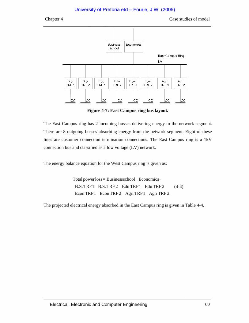
Chapter 4 Case studies of model
Electrical, Electronic and Computer Engineering 60
Figure 4-7: East Campus ring bus layout.
The East Campus ring has 2 incoming busses delivering energy to the network segment.
There are 8 outgoing busses absorbing energy from the network segment. Eight of these
lines are customer connection termination connections. The East Campus ring is a 1kV
connection bus and classified as a low voltage (LV) network.
The energy balance equation for the West Campus ring is given as:
+++
+++
−+=
2TRFAgri1TRFAgri2TRFEcon1TRFEcon2TRFEdu1TRFEdu2TRFB.S.1TRFB.S.
EconomicsschoolBusinesslosspowerTotal (4-4)
The projected electrical energy absorbed in the East Campus ring is given in Table 4-4.
UUnniivveerrssiittyy ooff PPrreettoorriiaa eettdd –– FFoouurriiee,, JJ WW ((22000055))
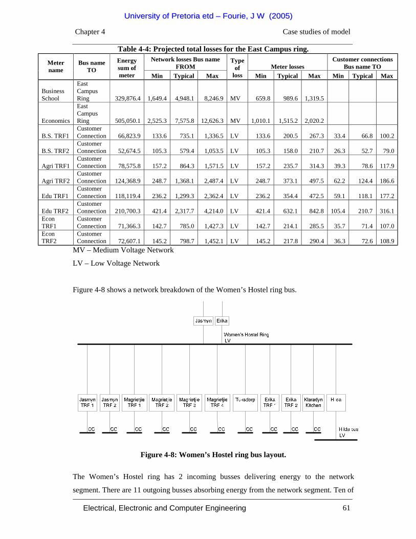
Chapter 4 Case studies of model
Electrical, Electronic and Computer Engineering 61
Table 4-4: Projected total losses for the East Campus ring. Network losses Bus name
FROM Meter losses Customer connections
Bus name TO Meter name
Bus name TO
Energy sum of meter Min Typical Max
Type of
loss Min Typical Max Min Typical Max
Business School
East Campus Ring 329,876.4 1,649.4 4,948.1 8,246.9 MV 659.8 989.6 1,319.5
Economics
East Campus Ring 505,050.1 2,525.3 7,575.8 12,626.3 MV 1,010.1 1,515.2 2,020.2
B.S. TRF1 Customer Connection 66,823.9 133.6 735.1 1,336.5 LV 133.6 200.5 267.3 33.4 66.8 100.2
B.S. TRF2 Customer Connection 52,674.5 105.3 579.4 1,053.5 LV 105.3 158.0 210.7 26.3 52.7 79.0
Agri TRF1 Customer Connection 78,575.8 157.2 864.3 1,571.5 LV 157.2 235.7 314.3 39.3 78.6 117.9
Agri TRF2 Customer Connection 124,368.9 248.7 1,368.1 2,487.4 LV 248.7 373.1 497.5 62.2 124.4 186.6
Edu TRF1 Customer Connection 118,119.4 236.2 1,299.3 2,362.4 LV 236.2 354.4 472.5 59.1 118.1 177.2
Edu TRF2 Customer Connection 210,700.3 421.4 2,317.7 4,214.0 LV 421.4 632.1 842.8 105.4 210.7 316.1
Econ TRF1
Customer Connection 71,366.3 142.7 785.0 1,427.3 LV 142.7 214.1 285.5 35.7 71.4 107.0
Econ TRF2
Customer Connection 72,607.1 145.2 798.7 1,452.1 LV 145.2 217.8 290.4 36.3 72.6 108.9
MV – Medium Voltage Network
LV – Low Voltage Network
Figure 4-8 shows a network breakdown of the Women’s Hostel ring bus.
Figure 4-8: Women’s Hostel ring bus layout.
The Women’s Hostel ring has 2 incoming busses delivering energy to the network
segment. There are 11 outgoing busses absorbing energy from the network segment. Ten of
UUnniivveerrssiittyy ooff PPrreettoorriiaa eettdd –– FFoouurriiee,, JJ WW ((22000055))

Chapter 4 Case studies of model
Electrical, Electronic and Computer Engineering 62
these lines are customer connection termination connections and one of the lines feed
busses lower down in the network layout. The Women’s Hostel ring is a 380 V connection
bus and classified as a low voltage (LV) network.
The energy balance equation for the Women’s Hostel ring is given as:
++++++
+++
−+=
HildaKitchenKlaradyn2TRFErika1TRFErikaTuksdorp4TRFMagrietjie3TRFMagrietjie
2TRFMagrietjie1TRFMagrietjie2TRFJasmyn1TRFJasmynErikaJasmynlosspowerTotal
(4-5)
The projected electrical energy absorbed in the Women’s Hostel ring is given in Table 4-5.
Table 4-5: Projected total losses for the East Campus ring.
Network losses Bus name FROM Meter losses
Customer connections Bus
name TO Meter name
Bus name TO
Energy sum of meter Min Typical Max
Type of
loss Min Typical Max Min Typical Max
Erika
Women's Hostel Ring 74,280.5 371.4 1,114.2 1,857.0 MV 148.6 222.8 297.1
Jasmyn
Women's Hostel Ring 221,624.3 1,108.1 3,324.4 5,540.6 MV 443.2 664.9 886.5
Jasmyn TRF1
Customer Connection 12,668.4 25.3 139.4 253.4 LV 25.3 38.0 50.7 6.3 12.7 19.0
Jasmyn TRF2
Customer Connection 23,485.8 47.0 258.3 469.7 LV 47.0 70.5 93.9 11.7 23.5 35.2
Magrietjie TRF1
Customer Connection 32,033.6 64.1 352.4 640.7 LV 64.1 96.1 128.1 16.0 32.0 48.1
Magrietjie TRF2
Customer Connection 8,276.0 16.6 91.0 165.5 LV 16.6 24.8 33.1 4.1 8.3 12.4
Magrietjie TRF3
Customer Connection 21,117.6 42.2 232.3 422.4 LV 42.2 63.4 84.5 10.6 21.1 31.7
Magrietjie TRF4
Customer Connection 39,757.6 79.5 437.3 795.2 LV 79.5 119.3 159.0 19.9 39.8 59.6
Tuksdorp Hilda ring 74,032.0 148.1 814.4 1,480.6 LV 148.1 222.1 296.1 Erika TRF1
Customer Connection 37,756.2 75.5 415.3 755.1 LV 75.5 113.3 151.0 18.9 37.8 56.6
Erika TRF2
Customer Connection 37,960.8 75.9 417.6 759.2 LV 75.9 113.9 151.8 19.0 38.0 56.9
Klaradyn Kitchen
Customer Connection 18,385.6 36.8 202.2 367.7 LV 36.8 55.2 73.5 9.2 18.4 27.6
Hilda Hilda ring 71,021.4 172.3 861.4 1,551.0 LV 90.7 453.5 816.3 18.0 90.2 162.0
Figure 4-9 shows a network breakdown of the Hilda ring bus.
UUnniivveerrssiittyy ooff PPrreettoorriiaa eettdd –– FFoouurriiee,, JJ WW ((22000055))

Chapter 4 Case studies of model
Electrical, Electronic and Computer Engineering 63
Figure 4-9: Hilda ring bus layout.
The Hilda ring has 1 incoming bus delivering energy to the network segment. There are 3
outgoing busses absorbing energy from the network segment. Three of these lines are
customer connection termination connections. The Hilda ring is a 380 V connection bus
and classified as a low voltage (LV) network.
The energy balance equation for the Hilda ring is given as:
( )AsterhofKitchenJasmynNieMyVergeetHildalosspowerTotal ++−= (4-6)
The projected electrical energy absorbed in the Hilda ring is given in Table 4-6.
Table 4-6: Projected total losses for the Hilda ring.
Network losses Bus name FROM Meter losses
Customer connections Bus
name TO Meter name Bus name TO Energy
sum of meter Min Typical Max
Type of
loss Min Typical Max Min Typical Max Hilda Hilda ring 71,021.4 172.28 861.4 1,551.0 LV 90.7 453.5 816.3 18 90.2 162 Vergeet My Nie
Customer Connection 24,651.8 49.3 271.2 493.0 LV 49.3 74.0 98.6 12.3 24.7 37.0
Jasmyn Kitchen
Customer Connection 19,275.5 38.6 212.0 385.5 LV 38.6 57.8 77.1 9.6 19.3 28.9
Asterhof Customer Connection 18,115.6 36.2 199.3 362.3 LV 36.2 54.3 72.5 9.1 18.1 27.2
The actual measured results shown in Table 4-7 were obtained from the electrical
distribution network layout as shown in Figure 4-2.
UUnniivveerrssiittyy ooff PPrreettoorriiaa eettdd –– FFoouurriiee,, JJ WW ((22000055))

Chapter 4 Case studies of model
Electrical, Electronic and Computer Engineering 64
Table 4-7: Total actual energy measured
Main/HB
bus
West
Campus
Ring
East
Campus
Ring
North
Campus
Ring
Women’s
Hostel
Ring
Hilda
Ring
Energy absorbed by
bus 3,752,637.7 533,628.1 795,236.1 826,526.3 305,473.6 71,021.4
Energy delivered. to
bus 3,756,023.6 686,291.6 834,926.4 962,404.9 305,904.8 74,032.2
% Difference of
energy absorbed. by
bus
0.09 28.61 4.99 16.44 0.14 4.24
% Difference of
energy delivered to
bus
0.09 22.24 4.75 14.12 0.14 4.07
% Difference
between energy
absorbed and
energy delivered
0 6.37 0.24 2.32 0 0.17
The difference in the energy absorbed and delivered must be less than 2.5 percent to be
acceptable. This acceptance level is a value determine by Eskom and the smaller the
acceptance level the higher the accuracy of the measured values. A percentage difference
level less than 10 % needs further investigation and levels higher than 10 % are
unacceptable.
The difference in the energy absorbed and delivered of the Main/HB bus, the East Campus
ring, the North Campus Ring, Women’s Hostel ring and the Hilda ring are less than 2%
and this means that the total amount of electrical energy delivered and absorbed in segment
of the electrical distribution network are acceptable. From Table 4-7 it can be concluded
that the West Campus ring needs investigation.
Table 4-8 shows the projected values as well as the percentage difference between the
projected energy absorbed and actual energy absorbed. One of the measures of identifying
the problem areas in an electrical distribution network is to compare the projected energy
UUnniivveerrssiittyy ooff PPrreettoorriiaa eettdd –– FFoouurriiee,, JJ WW ((22000055))

Chapter 4 Case studies of model
Electrical, Electronic and Computer Engineering 65
absorbed and the actual energy absorbed. If the percentage difference is less than 10 % the
difference is normal. A percentage difference less than 30 % is assumed high and values
higher than 30 % are abnormal. Table 4-8 shows that there is a high percentage difference
at the West Campus ring and the North Campus ring. The percentage difference between
the Main/HB bus, East Campus ring, Women’s Hostel ring and the Hilda ring could be
considered normal.
UUnniivveerrssiittyy ooff PPrreettoorriiaa eettdd –– FFoouurriiee,, JJ WW ((22000055))

Chapter 4 Case studies of model
Electrical, Electronic and Computer Engineering 66
Table 4-8: Calculated technical losses
Main/HB
bus
West
Campus
Ring
East
Campus
Ring
North
Campus
Ring
Women’s
Hostel
Ring
Hilda
Ring
Min 15,231.1 1,067.3 1,590.5 1,653.1 610.9 172.3
Typical 45,693.2 5,869.9 8,747.6 9,091.8 3,360.2 861.4 Total network
losses Max 76,155.4 10,672.6 15,904.7 16,530.5 6,109.5 1,550.5
Min 6,092.4 1,067.3 1,590.5 1,653.1 610.9 90.7
Typical 9,138.6 1,600.9 2,385.7 2,479.6 916.4 453.5 Meter losses
Max 12,184.9 2,134.5 3,180.9 3,306.1 1,221.9 816.3
Min 133.3 266.8 397.6 413.3 115.7 18.0
Typical 266.7 533.6 795.2 826.5 231.4 90.2
Customer
connection
losses Max 400.0 800.4 1,192.9 1,239.8 347.2 162.4
Min 18,780.1 6,862.9 8,349.3 9,624.0 2,959.0 73.7
Typical 46,950.3 10,294.4 12,523.9 14,436.1 4,438.6 368.4
Bus /
Transformer
losses Max 75,120.5 13,725.8 16,698.5 19,248.1 5,918.1 663.1
Min 3,680,903.1 672,565.8 818,227.9 943,156.8 299,986.7 66,628.8
Measured 3,756,023.6 686,291.6 834,926.4 962,404.9 305,904.7 74,032.1
Energy
delivered to
bus Max 3,831,144.1 700,017.4 851,624.9 981,653.0 309,822.9 81,435.2
Min 40,237.0 9,264.2 11,927.8 13,343.4 4,296.7 1,596.2
Typical 102,048.8 18,298.8 24,452.4 26,834.0 8,946.6 1,773.5 Projected total
loss for bus Max 163,860.7 27,333.3 36,977.0 40,324.5 13,596.6 1,950.9
Min 3,640,666.2 663,301.5 806,300.0 929,813.4 285,690.0 66,143.3
Typical 3,653,974.8 667,992.8 810,474.0 935,570.9 286,958.1 73,492.6
Projected
energy
absorbed Max 3,667,283.4 672,684.1 814,647.9 941,328.5 288,226.3 80,841.9
Min 3,677,585.0 522,955.5 779,331.4 809,995.7 299,364.1 63,919.3
Measured 3,752,637.7 533,628.1 795,236.1 826,526.3 305,473.6 71,021.4
Energy
absorbed by
bus Max 3,827,690.5 544,300.6 811,140.9 843,056.8 311,583.1 78,123.6
% Difference
between energy
absorbed and
energy
delivered
2.7 20.1 1.9 11.7 6.1 3.5
The typical value is the calculated value of the technical losses in the electrical distribution
network. The minimum and maximum values are calculated percentage values of the
typical value. This is done to be able to statistically calculate the problem areas in the
UUnniivveerrssiittyy ooff PPrreettoorriiaa eettdd –– FFoouurriiee,, JJ WW ((22000055))

Chapter 4 Case studies of model
Electrical, Electronic and Computer Engineering 67
distribution network. Another approach is to determine the minimum and maximum values
of the specific part of the network. This could however only be done if the minimum and
maximum values do not differ significantly from the typical value.
In both Table 4-7 and Table 4-8 the West Campus ring is identified as a segment with a
high percentage difference. This would identify the West Campus ring as a problem area.
The North Campus Ring is also identified as a problem area using Table 4-8 and therefore
it is identified as a potential problem area. Table 4-9 shows that the percentage difference
calculated for the projected losses in the electrical distribution network are equal
percentage values.
Table 4-9: Percentage difference of projected total losses
Main/HB
bus
West Campus
Ring
East Campus
Ring
North Campus
Ring
Women’s Hostel Ring
Hilda Ring
Total network losses 1.251 0.879 1.079 0.972 1.171 1.172 Meter losses 0.250 0.240 0.294 0.265 0.319 0.317 Customer connection losses 0.007 0.080 0.098 0.088 0.081 0.123 Bus / Transformer losses 1.285 1.541 1.545 1.543 1.547 1.501 Total projected percentage loss per bus 2.793 2.739 3.017 2.868 3.118 2.413
Using Table 4-9 a statistical approach is used in evaluating the different network segments
in the electrical distribution network. This statistical approach would identify the different
problem areas using structured mathematical techniques.
The calculation of the p value returns the two-tailed p value of a paired t test. The t test
generates a standard score value for each bus value with respect to the minimum, typical
and maximum value of each of the different busses on the electrical distribution network. It
returns a p value for each bus on the distribution using the two-tailed probability for the
normal distribution. This function is used to assess the likelihood that the actual measured
electrical energy output for a specific bus and the estimated electrical energy for the same
bus are derived from the same electrical energy input bus on the distribution network. A
small numerical p value indicates statistical significance in the t test.
The f test statistical function used in the model returns the one-tailed probability that the
variances in the actual measured electrical energy and the estimated electrical energy are
UUnniivveerrssiittyy ooff PPrreettoorriiaa eettdd –– FFoouurriiee,, JJ WW ((22000055))

Chapter 4 Case studies of model
Electrical, Electronic and Computer Engineering 68
not significantly different. This function is used to determine whether the measured and
estimated electrical energy have significantly different variances. A small numerical value
indicates statistical significance in the f test.
The confidence interval in the model calculates the mean of the bus of both the measured
and estimated electrical energy. It is used in the model to determine, with a particular level
of confidence the lowest and highest electrical energy level of use for a particular bus in
the electrical distribution network. This level of confidence is compared to the actual
measured value of the electrical energy used by the bus and the confidence interval should
be an order or more lower than the actual measured electrical energy to be assumed correct.
Table 4-10: Statistical evaluation
Main/HB
bus
West
Campus
Ring
East
Campus
Ring
North
Campus
Ring
Women’s
Hostel
Ring
Hilda
Ring
Determine p-value
for Paired t-test 0.10951 0.00066 0.15337 0.00324 0.02204 0.00005
Significance (f
test) 0.09260 0.12510 0.76200 0.22140 0.81700 0.02460
Standard deviation
of population 72,417.7 73,963.1 13,334.6 60,743.6 10,882.1 23,276.5
Confidence
interval for
population mean
47,314.3 102,838.2 7,772.4 73,012.6 10,172.2 38,737.9
Measured value of
bus 3752637.74 533628.06 795236.13 826526.26 305473.60 71021.43
These four statistical calculations can be subdivided into two groups namely statistical
calculations and measured data verification. The statistical evidence group contains the t-
test and f-test and the measured data verification group consists of the standard deviation
and the confidence interval. From these two groups the final potential problem area
identification is given in order of priority.
UUnniivveerrssiittyy ooff PPrreettoorriiaa eettdd –– FFoouurriiee,, JJ WW ((22000055))

Chapter 4 Case studies of model
Electrical, Electronic and Computer Engineering 69
The significant busses for the t-test are the West Campus ring, the North Campus ring and
the Hilda ring. The Women’s Hostel ring indicates a lesser significant level. The Main/HB
bus and the Woman’s hostel ring are identified as not significant, but this insignificance
could be as a result of problems lower down in the electrical distribution network.
Using the f-test as a measure of the different diversity in the projected energy absorbed and
actual energy absorbed in the electrical distribution network the Main/HB bus and the
Hilda ring are significant. A small level of significance is observed at the West Campus
ring and the North Campus ring. The busses that are not significant in the f-test evaluation
are the East Campus ring and the Women’s Hostel ring.
Comparing the t-test and the f-test as shown in Table 4-12 would yield that for the
electrical distribution network segment to be correct both tests must indicate a significant
level and visa versa. Table 4-11 shows the scale used to identify the different electrical
distribution network segments statuses.
Table 4-11: Scale used to identify statuses Column 1 Column 2 Decision
√ √ No problem — √ Potential problem × √ Problem area √ — Potential problem — — Problem area × — Problem area √ × Problem area — × Problem area × × Problem area
Key:
√ - significant statistical evidence,
— - small significance, and
× - not significant statistical evidence.
UUnniivveerrssiittyy ooff PPrreettoorriiaa eettdd –– FFoouurriiee,, JJ WW ((22000055))

Chapter 4 Case studies of model
Electrical, Electronic and Computer Engineering 70
Table 4-12: Statistical evidence t-test f-test
Main/HB bus × √ West Campus Ring √ — East Campus Ring × ×
North Campus Ring √ — Women’s Hostel Ring — ×
Hilda Ring √ √
Using Table 4-12 the following conclusions could be made using the statistical evidence
for the different network segments in the electrical distribution network:
Main/HB bus - problem area, but lower down in the network segment
West Campus ring - potential problem area
East Campus ring - problem area
North Campus ring - potential problem area
Women’s Hostel ring - potential problem area, possibly lower down in network segment
Hilda ring - no problem
The busses energy that are smaller than an order of the standard deviation of the network
segments area is the Main/HB bus, the West Campus ring, the East Campus ring, the North
Campus ring and the Women’s Hostel ring. This small order deviation of energy indicates
that the energy measured is correct. The Hilda ring is an order higher or in the same order
as the measured data indicating a problem area.
Using the confidence interval of the different network segments in the electrical
distribution network the Main/HB bus, East Campus ring, North Campus ring and the
Women’s Hostel ring is smaller than the measured energy in the specific network segment
indicating that the measured data values are correct. The West Campus ring and the Hilda
ring is in the same order as the measure energy absorbed for the specific segment and this
would be identified as a problem area.
Comparing the standard deviation and the confidence interval of the different network
segments are shown in Table 4-13.
UUnniivveerrssiittyy ooff PPrreettoorriiaa eettdd –– FFoouurriiee,, JJ WW ((22000055))

Chapter 4 Case studies of model
Electrical, Electronic and Computer Engineering 71
Table 4-13: Measuring data test
Standard deviation
Confidence interval
Main/HB bus √ √ West Campus Ring √ × East Campus Ring √ √
North Campus Ring √ √ Women’s Hostel Ring √ √
Hilda Ring × ×
Key:
√ - smaller than an order of the measured energy absorb in the network segment, and
× - greater than an order of the measured energy absorb in the network segment.
Using Table 4-13 the following conclusions could be made using the statistical evidence
for the different network segments in the electrical distribution network:
Main/HB bus - no problem
West Campus ring - potential problem area
East Campus ring - no problem
North Campus ring - no problem
Women’s Hostel ring - no problem
Hilda ring - potential problem area
The combined results of the statistical and measured data tests are given in Table 4-14.
Table 4-14: Combined results Statistical Measured
Main/HB bus — √ West Campus Ring √ — East Campus Ring × √
North Campus Ring √ √ Women’s Hostel Ring — √
Hilda Ring √ ×
Key:
√ - no problem,
— - potential problem area, and
× - problem area.
UUnniivveerrssiittyy ooff PPrreettoorriiaa eettdd –– FFoouurriiee,, JJ WW ((22000055))

Chapter 4 Case studies of model
Electrical, Electronic and Computer Engineering 72
Using Table 4-14 the following conclusions could be made using the statistical evidence
for the different network segments in the electrical distribution network. The results were
prioritized as follows:
1) Hilda ring – problem area
2) East Campus ring – problem area
3) West Campus ring – potential problem area
4) Woman’s Hostel ring – potential problem area on lower level
5) Main/HB bus – potential problem area on lower level
6) North Campus ring – no problem
The problem identification at the Women’s Hostel ring and the Main/HB bus should be
solved automatically as the lower order network segment problems are solved.
4.2 Verification of developed model in Garsfontein/Retriever
From an area in the Garsfontein region in Pretoria, South Africa electrical measured data
was used to verify whether the model developed could be used on a single line feeder.
Electrical measured data from the different lots feeding from the feeder were taken on
regular intervals and this data was used to verify the developed model. The electrical
distribution network at Garsfontein consists of one segment. Figure 4-10 shows the layout
of the Garsfontein network.
Figure 4-10: Layout at Garsfontein network
Figure 4-11 shows the detailed layout of the network in the electrical distribution network
of Garsfontein.
Garsfontein (Retriever) incomer
Metering points at different lots
UUnniivveerrssiittyy ooff PPrreettoorriiaa eettdd –– FFoouurriiee,, JJ WW ((22000055))

Chapter 4 Case studies of model
Electrical, Electronic and Computer Engineering 73
Figure 4-11: Detailed network layout.
The Retriever bus has a single incoming bus delivering energy to the network. There are 37
outgoing customer connections terminations that give electrical energy to households. The
Retriever bus is a 3.3kV connection bus and classified as a low voltage (LV) network.
The energy balance equation for the Retriever bus is given as:
++++++++++++++++++++++++++++++++++++
−=
no.2736Lot no.2735Lot no.2734Lot no.2733Lot no.2732Lot no.2798Lot no.2797Lot no.2796Lot no.2795Lot no.2794Lot no.2793Lot no.2792Lot no.2791Lot no.2790Lot no.2705Lot no.2704Lot no.2703Lot no.2702Lot no.2693Lot no.2692Lot no.2691Lot no.2690Lot no.2689Lot no.2688Lot no.2687Lot no.2686Lot no.2685Lot no.2684Lot no.2683Lot no.2682Lot no.2681Lot no.2680Lot no.2665Lot no.2664Lot no.2663Lot no.2662Lot no.2661Lot
RetrieverlosspowerTotal (4-7)
UUnniivveerrssiittyy ooff PPrreettoorriiaa eettdd –– FFoouurriiee,, JJ WW ((22000055))

Chapter 4 Case studies of model
Electrical, Electronic and Computer Engineering 74
The network segment calculates the projected losses of the network segment for a day,
week and month. The results of the different measured times in the network segment are
given in Table 4-15 to Table 4-20.
The projected electrical energy absorbed in the Retriever bus for a month is given in Table
4-15.
Table 4-15: Projected total losses for the different months on the Retriever bus. Network losses Bus name
FROM Meter losses Customer connections
Bus name TO Meter Name
Bus name TO
Energy sum of meter Min Typical Max
Type of
loss Min Typical Max Min Typical Max Retriever Month 1
Retriever bus 1 41,289.6 123.4 535.8 948.2 CC 162.3 243.4 324.5 20.6 41.3 61.9
Retriever Month 2
Retriever bus 2 39,085.0 118.6 510.9 903.1 CC 160.4 240.6 320.8 19.5 39.1 58.6
Retriever Month 3
Retriever bus 3 40,116.8 121.5 523.7 926.0 CC 162.9 244.4 325.8 20.1 40.1 60.2
Retriever Month 4
Retriever bus 4 40,469.0 121.9 527.0 932.2 CC 162.0 243.0 324.0 20.2 40.5 60.7
Retriever Month 5
Retriever bus 5 40,406.3 122.8 528.4 934.0 CC 167.6 251.4 335.2 20.2 40.4 60.6
Retriever Month 6
Retriever bus 6 39,931.5 101.6 482.6 863.7 CC 79.9 119.8 159.7 20.0 39.9 59.9
CC – Customer Connections
The projected electrical energy absorbed in the Retriever bus for a week is given in Table
4-16.
Table 4-16: Projected total losses for on a weekly base for the Retriever bus.
Network losses Bus name FROM Meter losses
Customer connections Bus
name TO Meter name Bus name TO
Energy sum of meter Min Typical Max
Type of
loss Min Typical Max Min Typical Max Retriever Week 1
Retriever bus 1 8896.2 27.0 116.3 205.6 CC 36.4 54.6 72.8 4.4 8.9 13.3
Retriever Week 2
Retriever bus 2 9009.1 27.6 118.2 208.8 CC 37.6 56.4 75.3 4.5 9.0 13.5
Retriever Week 3
Retriever bus 3 9526.1 28.7 124.1 219.5 CC 38.0 57.1 76.1 4.8 9.5 14.3
Retriever Week 4
Retriever bus 4 9222.2 23.2 110.9 198.7 CC 18.4 27.7 36.9 4.6 9.2 13.8
CC – Customer Connections
UUnniivveerrssiittyy ooff PPrreettoorriiaa eettdd –– FFoouurriiee,, JJ WW ((22000055))
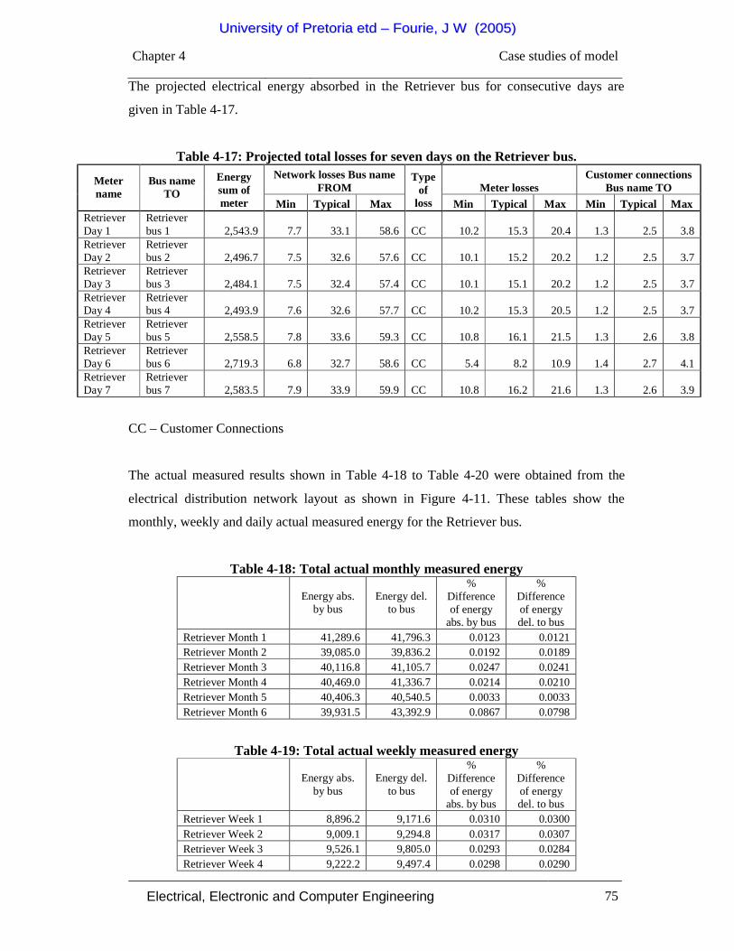
Chapter 4 Case studies of model
Electrical, Electronic and Computer Engineering 75
The projected electrical energy absorbed in the Retriever bus for consecutive days are
given in Table 4-17.
Table 4-17: Projected total losses for seven days on the Retriever bus. Network losses Bus name
FROM Meter losses Customer connections
Bus name TO Meter name
Bus name TO
Energy sum of meter Min Typical Max
Type of
loss Min Typical Max Min Typical Max Retriever Day 1
Retriever bus 1 2,543.9 7.7 33.1 58.6 CC 10.2 15.3 20.4 1.3 2.5 3.8
Retriever Day 2
Retriever bus 2 2,496.7 7.5 32.6 57.6 CC 10.1 15.2 20.2 1.2 2.5 3.7
Retriever Day 3
Retriever bus 3 2,484.1 7.5 32.4 57.4 CC 10.1 15.1 20.2 1.2 2.5 3.7
Retriever Day 4
Retriever bus 4 2,493.9 7.6 32.6 57.7 CC 10.2 15.3 20.5 1.2 2.5 3.7
Retriever Day 5
Retriever bus 5 2,558.5 7.8 33.6 59.3 CC 10.8 16.1 21.5 1.3 2.6 3.8
Retriever Day 6
Retriever bus 6 2,719.3 6.8 32.7 58.6 CC 5.4 8.2 10.9 1.4 2.7 4.1
Retriever Day 7
Retriever bus 7 2,583.5 7.9 33.9 59.9 CC 10.8 16.2 21.6 1.3 2.6 3.9
CC – Customer Connections
The actual measured results shown in Table 4-18 to Table 4-20 were obtained from the
electrical distribution network layout as shown in Figure 4-11. These tables show the
monthly, weekly and daily actual measured energy for the Retriever bus.
Table 4-18: Total actual monthly measured energy
Energy abs. by bus
Energy del. to bus
% Difference of energy
abs. by bus
% Difference of energy del. to bus
Retriever Month 1 41,289.6 41,796.3 0.0123 0.0121 Retriever Month 2 39,085.0 39,836.2 0.0192 0.0189 Retriever Month 3 40,116.8 41,105.7 0.0247 0.0241 Retriever Month 4 40,469.0 41,336.7 0.0214 0.0210 Retriever Month 5 40,406.3 40,540.5 0.0033 0.0033 Retriever Month 6 39,931.5 43,392.9 0.0867 0.0798
Table 4-19: Total actual weekly measured energy
Energy abs. by bus
Energy del. to bus
% Difference of energy
abs. by bus
% Difference of energy del. to bus
Retriever Week 1 8,896.2 9,171.6 0.0310 0.0300 Retriever Week 2 9,009.1 9,294.8 0.0317 0.0307 Retriever Week 3 9,526.1 9,805.0 0.0293 0.0284 Retriever Week 4 9,222.2 9,497.4 0.0298 0.0290
UUnniivveerrssiittyy ooff PPrreettoorriiaa eettdd –– FFoouurriiee,, JJ WW ((22000055))

Chapter 4 Case studies of model
Electrical, Electronic and Computer Engineering 76
Table 4-20: Total actual daily measured energy
Energy abs. by bus
Energy del. to bus
% Difference of energy
abs. by bus
% Difference of energy del. to bus
Retriever1 Day 1 2,537.3 2,588.3 0.0201 0.0197 Retriever1 Day 2 2,508.6 2,558.8 0.0200 0.0196 Retriever1 Day 3 2,503.3 2,553.4 0.0200 0.0196 Retriever1 Day 4 2,513.8 2,564.3 0.0201 0.0197 Retriever1 Day 5 2,568.7 2,621.0 0.0203 0.0199 Retriever1 Day 6 2,773.0 2,816.6 0.0157 0.0155 Retriever1 Day 7 2,587.9 2,640.6 0.0203 0.0199
The difference in the energy absorbed and delivered must be less than 2% to be acceptable.
This acceptance level is the predefined level determined by the user and the smaller the
acceptance level the higher the accuracy of the measured values. A percentage difference
level less than 10% needs further investigation and levels higher than 10% is unacceptable
meaning inaccurate input values.
The difference in the energy absorbed and delivered to the Retriever/Garsfontein region
based on the monthly, weekly and daily measured values over the period of time of all the
data under investigation is less than 2%. This means that the total amount of electrical
energy delivered and absorbed in segment of the electrical distribution network is
acceptable.
Table 4-21 to Table 4-23 shows the projected values as well as the percentage difference
between the projected energy absorbed and actual energy absorbed by the monthly, weekly
and daily measured values. One of the measures in identifying problem areas in the
electrical distribution network is to compare the projected energy absorbed and the actual
energy absorbed. If the percentage difference is less than 10% the difference is normal. A
percentage difference less than 30% is assumed high and values higher than 30% are
abnormal. Table 4-21 shows that there is no significant difference between the monthly
projected energy absorbed and the actual energy absorbed. The weekly and daily projected
energy absorbed and actual energy absorbed as shown in Table 4-22 and Table 4-23 shows
that the percentage difference is less than 10 percent in both cases and this could be
considered normal.
UUnniivveerrssiittyy ooff PPrreettoorriiaa eettdd –– FFoouurriiee,, JJ WW ((22000055))

Chapter 4 Case studies of model
Electrical, Electronic and Computer Engineering 77
Table 4-22: Calculated technical losses for the monthly values
Retriever
Month 1
Retriever
Month 2
Retriever
Month 3
Retriever
Month 4
Retriever
Month 5
Retriever
Month 6
Min 102.5 98.7 100.9 101.2 102.5 79.9
Typical 494.0 471.0 482.6 485.7 487.9 439.2
Total
network
losses Max 885.5 843.4 864.3 870.2 873.2 798.6
Min 162.3 160.4 162.9 162.0 167.6 79.9
Typical 243.4 240.6 244.4 243.0 251.4 119.8 Meter
losses Max 324.5 320.8 325.8 324.0 335.2 159.7
Min 20.6 19.5 20.1 20.2 20.2 20.0
Typical 41.3 39.1 40.1 40.5 40.4 39.9
Customer
connection
losses Max 61.9 58.6 60.2 60.7 60.6 59.9
Min 20.9 19.9 20.6 20.7 20.3 21.7
Typical 41.8 39.8 41.1 41.3 40.5 43.4
Bus /
Transformer
losses Max 62.7 59.8 61.7 62.0 60.8 65.1
Min 40,960.4 39,039.5 40,283.6 40,509.9 39,729.7 42,525.0
Measured 41,796.3 39,836.2 41,105.7 41,336.7 40,540.5 43,392.9
Energy
delivered to
bus Max 42,632.3 40,632.9 41,927.9 42,163.4 41,351.3 44,260.7
Min 306.3 298.6 304.4 304.1 310.6 201.4
Typical 820.5 790.5 808.2 810.5 820.2 642.4
Projected
total loss for
bus Max 1,334.7 1,282.5 1,312.0 1,316.9 1,329.8 1,083.3
Min 40,654.1 38,740.9 39,979.2 40,205.8 39,419.1 42,323.6
Typical 40,975.8 39,045.7 40,297.5 40,526.1 39,720.3 42,750.5
Projected
energy
absorbed Max 41,297.6 39,350.4 40,615.9 40,846.4 40,021.4 43,177.4
Min 40,463.8 38,303.3 39,314.4 39,659.7 39,598.2 39,132.9
Measured 41,289.6 39,085.0 40,116.8 40,469.0 40,406.3 39,931.5
Energy
absorbed
BY bus Max 42,115.4 39,866.7 40,919.1 41,278.4 41,214.4 40,730.2
Percentage
difference 0.8 0.1 0.4 0.1 1.7 6.6
UUnniivveerrssiittyy ooff PPrreettoorriiaa eettdd –– FFoouurriiee,, JJ WW ((22000055))

Chapter 4 Case studies of model
Electrical, Electronic and Computer Engineering 78
Table 4-23: Calculated technical losses for the weekly values
Retriever1
Week 1
Retriever1
Week 2
Retriever1
Week 3
Retriever1
Week 4
Min 22.4 22.9 23.8 18.4
Typical 107.2 108.9 114.3 101.4
Total
network
losses Max 191.9 194.9 204.8 184.4
Min 36.4 37.6 38.0 18.4
Typical 54.6 56.4 57.1 27.7 Meter
losses Max 72.8 75.3 76.1 36.9
Min 4.4 4.5 4.8 4.6
Typical 8.9 9.0 9.5 9.2
Customer
connection
losses Max 13.3 13.5 14.3 13.8
Min 4.6 4.6 4.9 4.7
Typical 9.2 9.3 9.8 9.5
Bus /
Transformer
losses Max 13.8 13.9 14.7 14.2
Min 8988.2 9108.9 9608.9 9307.4
Measured 9171.6 9294.8 9805.0 9497.4
Energy
delivered to
bus Max 9355.0 9480.7 10001.1 9687.3
Min 67.9 69.7 71.5 46.2
Typical 179.8 183.7 190.7 147.8
Projected
total loss for
bus Max 291.7 297.6 309.9 249.4
Min 8920.3 9039.2 9537.4 9261.2
Typical 8991.8 9111.2 9614.3 9349.6
Projected
energy
absorbed Max 9063.3 9183.1 9691.3 9437.9
Min 8718.2 8828.9 9335.6 9037.7
Measured 8896.2 9009.1 9526.1 9222.2
Energy
absorbed
BY bus Max 9074.1 9189.3 9716.6 9406.6
Percentage
difference 1.1 1.1 0.9 1.4
UUnniivveerrssiittyy ooff PPrreettoorriiaa eettdd –– FFoouurriiee,, JJ WW ((22000055))

Chapter 4 Case studies of model
Electrical, Electronic and Computer Engineering 79
Table 4-24: Calculated technical losses for the daily values
Retriever1
Day 1
Retriever1
Day 2
Retriever1
Day 3
Retriever1
Day 4
Retriever1
Day 5
Retriever1
Day 6
Retriever
1 Day 7
Min 6.4 6.3 6.3 6.3 6.5 5.4 6.6
Typical 30.5 30.0 29.9 30.1 31.0 29.9 31.2
Total
network
losses Max 54.7 53.8 53.5 53.8 55.4 54.4 55.9
Min 10.2 10.1 10.1 10.2 10.8 5.4 10.8
Typical 15.3 15.2 15.1 15.3 16.1 8.2 16.2
Meter losses Max 20.4 20.2 20.2 20.5 21.5 10.9 21.6
Min 1.3 1.2 1.2 1.2 1.3 1.4 1.3
Typical 2.5 2.5 2.5 2.5 2.6 2.7 2.6
Customer
connection
losses Max 3.8 3.7 3.7 3.7 3.8 4.1 3.9
Min 1.3 1.3 1.3 1.3 1.3 1.4 1.3
Typical 2.6 2.6 2.6 2.6 2.6 2.8 2.6
Bus /
Transformer
losses Max 3.9 3.8 3.8 3.8 3.9 4.2 4.0
Min 2,536.6 2,507.7 2,502.3 2,513.0 2,568.6 2,760.3 2,587.8
Measured 2,588.3 2,558.8 2,553.4 2,564.3 2,621.0 2,816.7 2,640.7
Energy
delivered to
bus Max 2,640.1 2,610.0 2,604.5 2,615.6 2,673.4 2,873.0 2,693.5
Min 19.1 18.9 18.9 19.1 19.9 13.6 20.0
Typical 51.0 50.2 50.1 50.5 52.3 43.6 52.7
Projected
total loss for
bus Max 82.8 81.5 81.3 81.9 84.7 73.6 85.3
Min 2,517.4 2,488.8 2,483.5 2,494.0 2,548.7 2,746.7 2,567.8
Typical 2,537.3 2,508.6 2,503.3 2,513.9 2,568.7 2,773.1 2,588.0
Projected
energy
absorbed Max 2,557.3 2,528.5 2,523.2 2,533.7 2,588.8 2,799.4 2,608.1
Min 2,493.0 2,446.8 2,434.4 2,444.0 2,507.3 2,664.9 2,531.8
Measured 2,543.9 2,496.7 2,484.1 2,493.9 2,558.5 2,719.3 2,583.5
Energy
absorbed
BY bus Max 2,594.8 2,546.7 2,533.8 2,543.8 2,609.7 2,773.7 2,635.2
Percentage
difference 0.3 0.5 0.8 0.8 0.4 1.9 0.2
In Tables 4-16 to Table 4-18 the percentage differences for the monthly, weekly and daily
values are less than 10 percent indicating that the energy usage for this residential area is
normal. Table 4-19 to Table 4-21 shows that the percentage difference calculated over the
UUnniivveerrssiittyy ooff PPrreettoorriiaa eettdd –– FFoouurriiee,, JJ WW ((22000055))

Chapter 4 Case studies of model
Electrical, Electronic and Computer Engineering 80
different periods for the projected losses in the electrical distribution network are almost
equal to the percentage values.
Table 4-24: Percentage monthly difference of projected total losses
Retriever Month 1
Retriever Month 2
Retriever Month 3
Retriever Month 4
Retriever Month 5
Retriever Month 6
Total network losses 1.206 1.206 1.198 1.198 1.228 1.027 Meter losses 0.594 0.616 0.606 0.600 0.633 0.280 Customer connection losses 0.101 0.100 0.100 0.100 0.102 0.093 Bus / Transformer losses 0.102 0.102 0.102 0.102 0.102 0.102 Total projected percentage loss per bus 2.002 2.025 2.006 2.000 2.065 1.503
Table 4-25: Percentage weekly difference of projected total losses
Retriever1 Week 1
Retriever1 Week 2
Retriever1 Week 3
Retriever1 Week 4
Total network losses 1.192 1.195 1.189 1.085 Meter losses 0.607 0.619 0.594 0.296 Customer connection losses 0.099 0.099 0.099 0.099 Bus / Transformer losses 0.102 0.102 0.102 0.102 Total projected percentage loss per bus 2.000 2.016 1.983 1.581
Table 4-26: Percentage daily difference of projected total losses
Retriever1 Day 1
Retriever1 Day 2
Retriever1 Day 3
Retriever1 Day 4
Retriever1 Day 5
Retriever1 Day 6
Retriever1 Day 7
Total network losses 1.204 1.197 1.194 1.196 1.205 1.079 1.207 Meter losses 0.603 0.604 0.605 0.610 0.628 0.294 0.626 Customer connection losses 0.100 0.100 0.099 0.099 0.100 0.098 0.100 Bus / Transformer losses 0.102 0.102 0.102 0.102 0.102 0.102 0.102 Total projected percentage loss per bus 2.009 2.002 2.000 2.007 2.035 1.572 2.035
Using Table 4-27 to Table 4-29 statistical approaches was used to evaluate the network
over a monthly, weekly and daily period in the electrical distribution network. This
statistical approach would identify the different problem areas using structured
mathematical techniques.
UUnniivveerrssiittyy ooff PPrreettoorriiaa eettdd –– FFoouurriiee,, JJ WW ((22000055))

Chapter 4 Case studies of model
Electrical, Electronic and Computer Engineering 81
The calculation of the p value returns the two-tailed p value of a paired t test. The t test
generates a standard score value for each bus value with respect to the minimum, typical
and maximum value of each of the different busses on the electrical distribution network. It
returns a p value for each bus on the distribution using the two-tailed probability for the
normal distribution. This function is used to assess the likelihood that the actual measured
electrical energy output for a specific bus and the estimated electrical energy for the same
bus are derived from the same electrical energy input bus on the distribution network. A
small numerical p value indicates statistical significance in the t test.
The f test statistical function used in the model returns the one-tailed probability that the
variances in the actual measured electrical energy and the estimated electrical energy are
not significantly different. This function is used to determine whether the measured and
estimated electrical energy have significantly different variances. A small numerical value
indicates statistical significance in the f test.
The standard deviation could not be calculated in this network segment layout as there is
only one bus and therefore the deviation if been calculated will tend to infinite. The
confidence interval in the model calculates the mean of the bus of both the measured and
estimated electrical energy. It is used in the model to determine, with a particular level of
confidence the lowest and highest electrical energy level of use for a particular bus in the
electrical distribution network. This level of confidence is compared to the actual measured
value of the electrical energy used by the bus and the confidence interval should be an
order or more lower than the actual measured electrical energy to be assumed correct. As
there is only one bus under investigation the confidence interval is large. These results
therefore are also omitted in the determination of the problem areas for the particular time
interval.
Table 4-27: Statistical evaluation of the monthly data
Retriever Month 1
Retriever Month 2
Retriever Month 3
Retriever Month 4
Retriever Month 5
Retriever Month 6
Determine p-value for Paired t-test 0.5987 0.8254 0.9820 0.8993 0.2396 0.3537 Significance (ftest) 586.27 531.07 554.83 551.42 662.35 1646.82 Confidence interval for population mean 41289.59 39084.97 40116.78 40469.03 40406.30 39931.52 Measured value of bus 41796.33 39836.21 41105.74 41336.65 40540.47 43392.88
UUnniivveerrssiittyy ooff PPrreettoorriiaa eettdd –– FFoouurriiee,, JJ WW ((22000055))
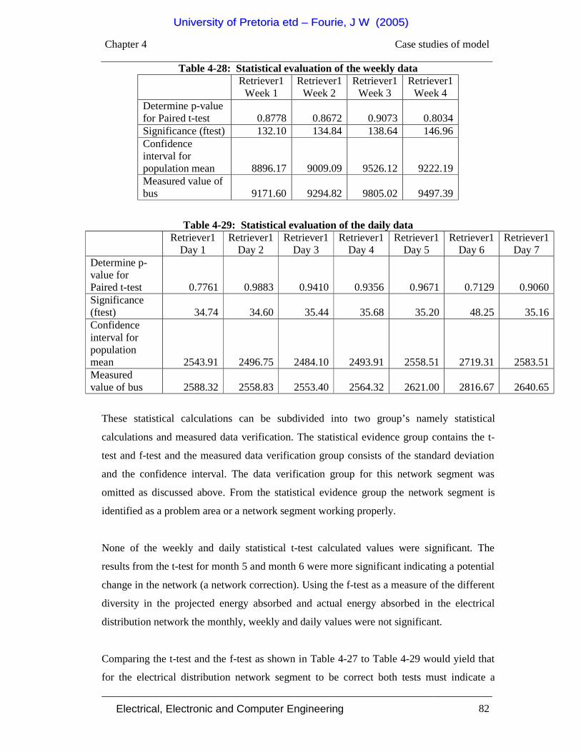
Chapter 4 Case studies of model
Electrical, Electronic and Computer Engineering 82
Table 4-28: Statistical evaluation of the weekly data
Retriever1
Week 1 Retriever1
Week 2 Retriever1
Week 3 Retriever1
Week 4 Determine p-value for Paired t-test 0.8778 0.8672 0.9073 0.8034 Significance (ftest) 132.10 134.84 138.64 146.96 Confidence interval for population mean 8896.17 9009.09 9526.12 9222.19 Measured value of bus 9171.60 9294.82 9805.02 9497.39
Table 4-29: Statistical evaluation of the daily data
Retriever1
Day 1 Retriever1
Day 2 Retriever1
Day 3 Retriever1
Day 4 Retriever1
Day 5 Retriever1
Day 6 Retriever1
Day 7 Determine p-value for Paired t-test 0.7761 0.9883 0.9410 0.9356 0.9671 0.7129 0.9060 Significance (ftest) 34.74 34.60 35.44 35.68 35.20 48.25 35.16 Confidence interval for population mean 2543.91 2496.75 2484.10 2493.91 2558.51 2719.31 2583.51 Measured value of bus 2588.32 2558.83 2553.40 2564.32 2621.00 2816.67 2640.65
These statistical calculations can be subdivided into two group’s namely statistical
calculations and measured data verification. The statistical evidence group contains the t-
test and f-test and the measured data verification group consists of the standard deviation
and the confidence interval. The data verification group for this network segment was
omitted as discussed above. From the statistical evidence group the network segment is
identified as a problem area or a network segment working properly.
None of the weekly and daily statistical t-test calculated values were significant. The
results from the t-test for month 5 and month 6 were more significant indicating a potential
change in the network (a network correction). Using the f-test as a measure of the different
diversity in the projected energy absorbed and actual energy absorbed in the electrical
distribution network the monthly, weekly and daily values were not significant.
Comparing the t-test and the f-test as shown in Table 4-27 to Table 4-29 would yield that
for the electrical distribution network segment to be correct both tests must indicate a
UUnniivveerrssiittyy ooff PPrreettoorriiaa eettdd –– FFoouurriiee,, JJ WW ((22000055))

Chapter 4 Case studies of model
Electrical, Electronic and Computer Engineering 83
significant level and visa versa. From these statistical results the daily and weekly
measured values seems to be inaccurate and no statistical evidence could be found to
conclude that the network segment is operating correctly. For the monthly data the
measured values are more accurate over a longer period of time and data collected over a
month is the shortest time that could be used to identify potential problem areas. As new
meters were installed in month 5 and month 6 the data collected for these months indicates
a high level of significance, indicating that the network problems are solved of the first
four months.
UUnniivveerrssiittyy ooff PPrreettoorriiaa eettdd –– FFoouurriiee,, JJ WW ((22000055))

Electrical, Electronic and Computer Engineering 84
CHAPTER 5: CONCLUSIONS
5.1 Introduction
The main objective of this dissertation was discussed in chapter 1 and included a subset of
specific objectives. This chapter will conclude with the value of the developed strategy as
well as recommendation regarding future work based on the dissertation.
5.2 Conclusion on the objectives
The main objective of this dissertation was to develop a strategy to minimize electrical
energy losses. To derive a strategy a model was constructed to identify the problem areas
in an electricity distribution network and this was used to develop a strategy to minimize
electricity losses in an electricity distribution network. The model calculated the technical
losses and used it to derive the non-technical losses in the electricity distribution network.
In evaluating an electrical distribution network technical and economical grounds were
used. The technical evaluation was done on distribution feeders that supply customers with
electricity and these distribution feeders were used to ensure continuity and quality of
service. The economical performance of a distribution network was evaluated by the ratio
of the amount of electricity delivered to the customer and the global cost of the electricity
distribution network. This dissertation used the technical evaluation ground to develop a
strategy that identified the different problem areas in an electrical distribution network. By
solving these problem areas the technical evaluation improved and the amount of
electricity delivered to the customer increased, therefore improving the economical benefit
of the customer. The main objective was achieved by addressing a series of specific
objectives.
• Conclusion on the model constructed to determine the technical losses
An indirect approach was used to calculate the technical losses to be able to use a
minimum amount of parameters needed from the field. The calculation of the technical
losses in the model was calculated using a percentage estimation of the loss parameters
defined for the different segments in the distribution network. The percentage
UUnniivveerrssiittyy ooff PPrreettoorriiaa eettdd –– FFoouurriiee,, JJ WW ((22000055))

Chapter 5 Conclusions
Electrical, Electronic and Computer Engineering 85
calculations in the model define a minimum and maximum percentage parameter for
the different network segments in the distribution network. These parameters are used
to calculate the losses of each segment in the electrical distribution network as a
percentage of the input electrical energy to the network segment.
• Conclusion on determining a method to calculate the non-technical losses
As discussed in chapter 3 non-technical losses in distribution networks cannot be
calculated as these losses are due to human intervention in the distribution network.
This was shown using the model developed for the determination of electrical energy
losses in an electrical distribution network. Therefore the total electrical energy
supplied to the distribution network includes the non-technical losses as a parameter.
• Conclusion on determining a procedure to identify the problem areas
Problem areas were identified using the statistical methods as discussed in chapter 3.
The investigation of the problem areas and the problem solving of the areas was done
using inspection teams finding the causes of the electrical losses in electrical
distribution network. As problems are identified in the problem areas procedures are
followed to correct the different problems.
• Conclusion on constructing a matrix to prioritize the problem areas
In chapter 4, four statistical calculations were used to determine a matrix in order to
prioritize the problem areas in an electrical distribution network. The four statistical
calculations were subdivided into two groups and from these two groups the final
potential problem area identification was given in order of priority.
Addressing the specific objectives has ensured that all material necessary to meet the main
objective has been covered. Energy supply companies will definitely benefit if they
implement this strategy to minimize electrical energy losses in an electrical distribution
network as it will identify the problem areas more accurately than currently been done.
Using the procedures identified in the dissertation will ensure an effective identification of
problem areas and rectifying the problems. It can be concluded that with the strategy
UUnniivveerrssiittyy ooff PPrreettoorriiaa eettdd –– FFoouurriiee,, JJ WW ((22000055))

Chapter 5 Conclusions
Electrical, Electronic and Computer Engineering 86
developed in this dissertation electrical supply companies will be able to estimate energy
losses in their electrical distribution networks. They will surely benefit from these
reductions in energy generation and system capacity as well as, reductions will occur in the
cost of energy to the consumer.
5.3 Conclusions at the main campus of the University of Pretoria
The results obtain from the measured electrical data at the main campus of the University
of Pretoria was used to proof that the model can identify potential problems in the
electrical distribution network. In chapter 4 table 4-12 and table 4-13 were used to
conclude that using the statistical evidence for the different network segments in the
electrical distribution network problem areas in the electrical distribution network could be
identified. The results from chapter 4 are prioritized as follows:
1) Hilda ring – problem area
2) East Campus ring – problem area
3) West Campus ring – potential problem area
4) Woman’s Hostel ring – potential problem area on lower level
5) Main/HB bus – potential problem area on lower level
6) North Campus ring – no problem
The problem identification at the Women’s Hostel ring and the Main/HB bus should be
solved automatically as the lower order network segment problems are solved. It is
therefore concluded that the model develop could identify potential problems in the
electrical distribution network and a strategy could then be derived to resolve the problems.
5.4 Conclusions at the Tshwane Metropolitan Council
The aim of this case study was to determine the minimum period that would be sufficient
to identify a potential problem in an electrical distribution network. The results obtained
from the Tshwane Metropolitan Council indicate that the weekly and daily statistical t-test
calculations were inconclusive because of the short period of time that the energy was
UUnniivveerrssiittyy ooff PPrreettoorriiaa eettdd –– FFoouurriiee,, JJ WW ((22000055))

Chapter 5 Conclusions
Electrical, Electronic and Computer Engineering 87
monitored. Using the f-test over the different periods of time as a measure of the different
diversity in the projected energy absorbed and actual energy absorbed in the electrical
distribution network the monthly, weekly and daily values were not significant.
Comparing the t-test and the f-test as shown in Table 4-27 to Table 4-29 the statistical
results of the daily and weekly measured values seems to be inaccurate and no statistical
evidence could be found to conclude that the network segment is operating correctly. For
the monthly data the measured values are more accurate over a longer period of time and it
can be concluded that the data collected over a month is the shortest period of time that
could be used to identify potential problem areas in a electrical distribution network.
5.5 Recommendation and Future work
This section includes a recommendation for using the strategy developed in energy
management programs as well as defining the scope for future work based on this material.
5.5.1. Recommendation on the integration of the strategy into energy management
programs
The starting point when looking at the strategy to minimize energy losses must be to
determine the extent of the losses in the electrical distribution network. If no method is
presently used to identify losses then a new action plan should be discussed using the
model developed in this dissertation. Senior management in the energy management
department should discuss this action plan and get line managers as well as employees
involved in the initiative to get the electrical energy losses decreased.
The next step is to identify the electrical network layout as accurately as possible. With the
network layout not correctly identified the model developed will not identify sections
operating correctly. This network layout could then be used as the input for the model and
the data can be collected and analyzed using the strategy presented in this dissertation.
The integral part of using the model and saving electrical energy is the plan to solve the
problem areas. Management support and a plan to solve the potential problems areas is
UUnniivveerrssiittyy ooff PPrreettoorriiaa eettdd –– FFoouurriiee,, JJ WW ((22000055))

Chapter 5 Conclusions
Electrical, Electronic and Computer Engineering 88
vital in the practical implementation of the strategy to ensure that as soon as the problem
area is identified by the model that the necessary actions are taken to ensure that the
problem are been resolved.
5.5.2. Future work
If this dissertation had to be rewritten based on existing knowledge and experience,
nothing would be changed. The length of this dissertation may be longer as more case
studies would be included to reiterate the working of the strategy to minimize the electrical
losses in an electrical distribution network. The purpose of this dissertation was to develop
a strategy to minimize the electrical losses in an electrical distribution network and
therefore the electrical data obtained from the University of Pretoria and Tshwane
Metropolitan Council was used to identify problem areas and to develop the strategy to
minimize electrical losses.
An area that could be investigated further is the possibility to expand the strategy to water
networks and production line networks. These networks could be investigated as this
dissertation can be implemented in every area that is energy related.
UUnniivveerrssiittyy ooff PPrreettoorriiaa eettdd –– FFoouurriiee,, JJ WW ((22000055))

Electrical, Electronic and Computer Engineering 89
REFERENCES
[1] N Mohan, Y Undeland, and PR Robbins, Power Electronics: Converters,
Applications, and Design, p. 415-417, 1995.
[2] IE Davidson and A Odubiyi, Technical loss computation and economic dispatch
model for T&D systems in deregulated ESI, Power Engineering Journal, p 55, 2002.
[3] N Krishnaswamy, A holistic approach to practical techniques to analysis and reduce
technical losses on Eskom power networks using the principles of management of
technologies, Management of technology, Technology leadership program, p 28-33,
2000.
[4] T Chen and S Wang, Applications of simplified bidirectional feeder models for
accelerating the voltage drop and power loss calculations, National Taiwan Institute
of Technology, p 734-739, 1995.
[5] World Bank Group, Efficient use of energy:World bank group, Pollution prevention
and abatement handbook, 1998.
[6] I Lane, JJ Hoogenboezem, and GJ Delport, The present and future of national
electricity demand, Domestic Use of Electrical Energy Conference, 1997.
[7] RJ Scholes and MR Van Der Merwe, Greenhouse Gas Inventor, p 63, 1993.
[8] DC Neethling and RK Dutkiewicz, International and regional energy policy
development, focusing on end use of energy, Enerconomy, p 93, 1993.
[9] HM Khodr and JA Molea, Standarization of technical losses in primary circuits of
distribution for scada application, IEEE transactions on power delivery, p 172-173,
2001.
UUnniivveerrssiittyy ooff PPrreettoorriiaa eettdd –– FFoouurriiee,, JJ WW ((22000055))

References
Electrical, Electronic and Computer Engineering 90
[10] N Mohan, N, TM Undeland and WP Robbins, Power electronics converters,
applications and design, 2nd Edition, John Wiley and sons inc, New York, p 732,
1995.
[11] N Mohan, N, TM Undeland and WP Robbins, Power electronics converters,
applications and design, 2nd Edition, John Wiley and sons inc, New York, p 752,
1995.
[12] PC Sen, Priciples of electric machines and power electronics, 2nd edition, John
Wiley and sons, New York, p 54, 1996.
[13] P Horowitz and W Hill, The art of electronics, 2nd edition, Cambrigde:Univeristy
Press, Cambrigde, p 220, 1995.
[14] F Nortje, Electrification technical losses management system, Vector, p 4-6, 1995.
[15] RO Ferrera and PJ Paoletich, Model for losses calculation and breakdown in
distribution systems, CIRED2001, p 5.34, 2001.
[16] JJ Grainger and TJ Kendrew, Evaluation of technical losses on electric distribution
systems, CIRED, p 488-493, 1989.
[17] CCB Oliveira and N Kagan, A new method for the computation of technical losses in
electrical power distribution systems, IEE CIRED 2001, p 482, 2001.
[18] H Kerzner, Project management a systems approach to planning, scheduling, and
controlling, 5th edition, Van Nostrand Reinhold Publishers, New York, p 458-466,
1995.
[19] JE Calmeyer, The management of electricity cost within an academic institution,
Masters dissertation in Electrical Engineering, University of Pretoria, RSA, p 27,
1999.
UUnniivveerrssiittyy ooff PPrreettoorriiaa eettdd –– FFoouurriiee,, JJ WW ((22000055))

References
Electrical, Electronic and Computer Engineering 91
[20] G Schreyogg and H Steinmann, Strategic control: A new perspective, Academy of
management review 12, p 96, 1987.
[21] G Douglas, GC Montgomery and NH Runger, Engineering Statistics, John Wiley and
Sons, Arizona State University, p 140-151, 2000.
[22] IsiXSigma homepage
http://www.isixsigma.com/dictionary/pairttest.htm
[23] Snedecor and Cochran
http://www.itl.nist.gov/div898/handbook/eda/section4/eda43.htm#Snedecor
[24] Psycho.uni-duesseldorf
http://www.psycho.uni-duesseldorf.de/aap/projects/gpower/literature.html
[25] RM Surtees, The impact of electrification on the electricity demand profile. Domestic
Use of Electrical Energy Conference, RSA, p 265, 1993.
UUnniivveerrssiittyy ooff PPrreettoorriiaa eettdd –– FFoouurriiee,, JJ WW ((22000055))

Electrical, Electronic and Computer Engineering 92
Appendix A: General module Source Code
Source code for general module: Public Sub ModelCalc()
ApplyFormat CalcBusValues CalcLosses Correlation Statistics filedatagenerate
End Sub Sub transformers() ''Determine if their are transformers on the bus 'Move to correct sheet Sheets("MeterParameters").Select Range("A1").Select 'Get meter names for busses on simulation Dim counter As Integer 'counter for array counter = Sheets("RingMatrix").Range("E1").value Dim BusNames(65000, 5) As String 'array of meter names and connection on network Dim testvalue(3) As String 'test value of bus Dim LossValues(65000, 9) As Double 'Values of losses of network, meter, and customer Dim LostTest(9) As Double i = 0 h = 0 BusNames(i, 1) = "" BusNames(i, 2) = "" Dim valueadd As Boolean valueadd = False For x = 1 To counter 'Meters bus name FROM testvalue(1) = ActiveCell.Offset(1 + x, 1).Range("A1").value testvalue(2) = ActiveCell.Offset(1 + x, 2).Range("A1").value testvalue(3) = ActiveCell.Offset(1 + x, 3).Range("A1").value 'Get the test values of the losses into a test array For a = 1 To 3 LostTest(a) = ActiveCell.Offset(1 + x, 4 + a).Range("A1").value Next a For a = 4 To 9LostTest(a) = ActiveCell.Offset(1 + x, 5 + a).Range("A1").value Next a For j = 0 To i If (testvalue(1) = BusNames(j, 1)) And (testvalue(1) <> testvalue(2)) Then
UUnniivveerrssiittyy ooff PPrreettoorriiaa eettdd –– FFoouurriiee,, JJ WW ((22000055))

Appendix A General module Source Code
Electrical, Electronic and Computer Engineering 93
valueadd = True For a = 1 To 9 LossValues(i, a) = LossValues(i, a) + LostTest(a) Next a End If Next j If (valueadd = False) And (testvalue(1) <> testvalue(2)) Then i = i + 1 BusNames(i, 1) = testvalue(1) BusNames(i, 2) = testvalue(3) For a = 1 To 9 LossValues(i, a) = LostTest(a) Next a Else valueadd = False End If For j = 0 To h If (testvalue(2) = BusNames(j, 3)) And (testvalue(1) <> testvalue(2)) Then valueadd = True End If Next j If valueadd = False And testvalue(1) <> testvalue(2) Then Module5 - 2 h = h + 1 BusNames(h, 3) = testvalue(2) BusNames(h, 4) = testvalue(3) Else valueadd = False End If Next x If i = h Then For j = 1 To i For k = 1 To i If (BusNames(j, 1) = BusNames(k, 3) And BusNames(j, 2) = BusNames(k, 4)) Then BusNames(j, 5) = "CC" Else If (BusNames(j, 1) = BusNames(k, 3) And BusNames(j, 2) <> BusNames(k, 4)) Then If (BusNames(j, 2) = "ST" Or BusNames(j, 4) = "ST") Then BusNames(j, 5) = "DS" Else If (BusNames(j, 2) = "MV" Or BusNames(j, 4) = "MV") Then BusNames(j, 5) = "DT" Else If (BusNames(j, 2) = "LV" Or BusNames(j, 4) = "LV") Then BusNames(j, 5) = "CC" End If End If End If End If
UUnniivveerrssiittyy ooff PPrreettoorriiaa eettdd –– FFoouurriiee,, JJ WW ((22000055))

Appendix A General module Source Code
Electrical, Electronic and Computer Engineering 94
End If Next k Next j Else ending "RingMatrix", "Fault in bus setup. Please revise your setup." End If 'Move to correct sheet Sheets("RingMatrix").Select Range("A1").Select For j = 1 To i ActiveCell.Offset(j, 10).Range("A1").value = BusNames(j, 5) Next j 'Move to correct sheet Sheets("Correlation").Select Range("A1").Select For j = 1 To i ActiveCell.Offset(1 + j, 0).Range("A1").value = BusNames(j, 1) For a = 1 To 9 ActiveCell.Offset(1 + j, a).Range("A1").value = LossValues(j, a) Next a Next j End Sub Sub ApplyFormat() 'Clear all data clearall Dim workdir As String 'Working directory for the simulation workdir = Sheets("procedure and macros").Range("F1").value + "\" 'Copy the MeterParameter values to RingMatrix sheet Sheets("MeterParameters").Select Range("A3:C3").Select Range(Selection, Selection.End(xlDown)).Select Selection.Copy Sheets("RingMatrix").Select Range("A2").Select Selection.PasteSpecial Paste:=xlValues, Operation:=xlNone, SkipBlanks:= _ False, Transpose:=False 'Move to correct sheet Sheets("RingMatrix").Select Range("A1").Select 'Get meter names Dim MyArray(65000) As String 'array of meter names Dim counter As Integer 'counter for array counter = Sheets("RingMatrix").Range("E1").value - 1
UUnniivveerrssiittyy ooff PPrreettoorriiaa eettdd –– FFoouurriiee,, JJ WW ((22000055))

Appendix A General module Source Code
Electrical, Electronic and Computer Engineering 95
For x = 0 To counter MyArray(x) = ActiveCell.Offset(1 + x, 0).Range("A1").value Next x 'Enter headings Sheets("RingMatrix").Select Range("A2").Select Range(Selection, Selection.End(xlDown)).Select Range(Selection, Selection.End(xlDown)).Select Selection.Copy Sheets("Data").Select Selection.PasteSpecial Paste:=xlAll, Operation:=xlNone, SkipBlanks:=True _ , Transpose:=True Range("A2").Select 'Move to correct sheet Sheets("Data").Select 'Sheet name Range("A2").Select 'Move to correct position 'Get external text files into sheet For x = 0 To counter With ActiveSheet.QueryTables.Add(Connection:= _ "TEXT;" + workdir + MyArray(x) + ".txt", _ Destination:=ActiveCell) .name = MyArray(x) .FieldNames = True .RowNumbers = False .FillAdjacentFormulas = False .PreserveFormatting = True .RefreshOnFileOpen = True .RefreshStyle = xlOverwriteCells .SavePassword = False .SaveData = True .AdjustColumnWidth = True .RefreshPeriod = 50 .TextFilePromptOnRefresh = False .TextFilePlatform = xlWindows .TextFileStartRow = 1 .TextFileParseType = xlDelimited .TextFileTextQualifier = xlTextQualifierDoubleQuote .TextFileConsecutiveDelimiter = False .TextFileTabDelimiter = True .TextFileSemicolonDelimiter = False .TextFileCommaDelimiter = False .TextFileSpaceDelimiter = False .TextFileColumnDataTypes = Array(9, 1, 9, 9, 9, 9) .Refresh BackgroundQuery:=False End With ActiveCell.Offset(0, 1).Range("A1").Select Next x
UUnniivveerrssiittyy ooff PPrreettoorriiaa eettdd –– FFoouurriiee,, JJ WW ((22000055))

Appendix A General module Source Code
Electrical, Electronic and Computer Engineering 96
'Enter headings Sheets("RingMatrix").Select Range("A2").Select Range(Selection, Selection.End(xlDown)).Select Range(Selection, Selection.End(xlDown)).Select Selection.Copy Sheets("DataCalc").Select Selection.PasteSpecial Paste:=xlAll, Operation:=xlNone, SkipBlanks:=True _ , Transpose:=True Range("A2").Select 'Calculate the sum For x = 0 To counter ActiveCell.FormulaR1C1 = "=SUM(Data!RC:R[65534]C)" ActiveCell.Offset(0, 1).Range("A1").Select Next x 'Copy values of meter sums to RingMatrix Range("A2").Select Range(Selection, Selection.End(xlToRight)).Select Selection.Copy Sheets("RingMatrix").Select Range("D2").Select Selection.PasteSpecial Paste:=xlValues, Operation:=xlNone, SkipBlanks:= _ False, Transpose:=True 'Copy meters to monthsheet Sheets("RingMatrix").Select Range("A2").Select Range(Selection, Selection.End(xlDown)).Select Selection.Copy Sheets("Month checksheet").Select Selection.PasteSpecial Paste:=xlValues, Operation:=xlNone, SkipBlanks:= _ False, Transpose:=False Range("B6:C61").Select Application.CutCopyMode = False Selection.Borders(xlDiagonalDown).LineStyle = xlNone Selection.Borders(xlDiagonalUp).LineStyle = xlNone With Selection.Borders(xlEdgeLeft) .LineStyle = xlContinuous .Weight = xlThin .ColorIndex = xlAutomatic End With With Selection.Borders(xlEdgeTop) .LineStyle = xlContinuous .Weight = xlThin .ColorIndex = xlAutomatic End With With Selection.Borders(xlEdgeBottom)
UUnniivveerrssiittyy ooff PPrreettoorriiaa eettdd –– FFoouurriiee,, JJ WW ((22000055))

Appendix A General module Source Code
Electrical, Electronic and Computer Engineering 97
.LineStyle = xlContinuous
.Weight = xlThin
.ColorIndex = xlAutomatic End With With Selection.Borders(xlEdgeRight) .LineStyle = xlContinuous .Weight = xlThin .ColorIndex = xlAutomatic End With With Selection.Borders(xlInsideVertical) .LineStyle = xlContinuous .Weight = xlThin .ColorIndex = xlAutomatic End With With Selection.Borders(xlInsideHorizontal) .LineStyle = xlContinuous .Weight = xlThin .ColorIndex = xlAutomatic End With Range("A1:G1").Select Range(Selection, Selection.End(xlDown)).Select Range(Selection, Selection.End(xlDown)).Select Range(Selection, Selection.End(xlDown)).Select ActiveSheet.PageSetup.PrintArea = "$A:$G" ending "RingMatrix", "All data files imported" End Sub Sub CalcBusValues() Dim workdir As String 'Working directory for the simulation workdir = Sheets("procedure and macros").Range("F1").value + "\" 'Move to correct sheet Sheets("RingMatrix").Select Range("A1").Select 'Get meter names for busses on simulation Dim counter As Integer 'counter for array counter = Sheets("RingMatrix").Range("E1").value - 1 Dim BusNames(65000) As String 'array of meter names Dim BusValue(65000, 2) As Double 'array of meter values Dim testvalue As String 'test value of bus i = 0 BusNames(i) = "" Dim valueadd As Boolean Dim test As Double valueadd = False For x = 0 To counter 'Meters bus name FROM testvalue = ActiveCell.Offset(1 + x, 1).Range("A1").value test = ActiveCell.Offset(1 + x, 3).Range("A1").value For j = 0 To i If testvalue = BusNames(j) Then
UUnniivveerrssiittyy ooff PPrreettoorriiaa eettdd –– FFoouurriiee,, JJ WW ((22000055))

Appendix A General module Source Code
Electrical, Electronic and Computer Engineering 98
BusValue(j, 1) = BusValue(j, 1) + test valueadd = True End If Next j If valueadd = False Then i = i + 1 BusNames(i) = testvalue BusValue(i, 1) = test Else valueadd = False End If Next x 'Calculate the sum of the bus For x = 0 To counter 'Meters bus name TO testvalue = ActiveCell.Offset(1 + x, 2).Range("A1").value test = ActiveCell.Offset(1 + x, 3).Range("A1").value For j = 0 To i If testvalue = BusNames(j) Then BusValue(j, 2) = BusValue(j, 2) + test valueadd = True End If Next j If valueadd = False Then i = i + 1 BusNames(i) = testvalue BusValue(i, 1) = test Else valueadd = False End If Next x For j = 1 To i ActiveCell.Offset(j, 6).Range("A1").value = BusNames(j) ActiveCell.Offset(j, 7).Range("A1").value = BusValue(j, 1) ActiveCell.Offset(j, 8).Range("A1").value = BusValue(j, 2) Next j 'Difference for power delevired - power absorbed by system ActiveCell.Offset(1, 9).Range("A1").Select ActiveCell.FormulaR1C1 = "=RC[-1]-RC[-2]" Selection.Copy ActiveCell.Offset(0, -1).Range("A1").Select Selection.End(xlDown).Select ActiveCell.Offset(0, 1).Range("A1").Select Range(Selection, Selection.End(xlUp)).Select ActiveSheet.Paste ''Calculate % difference of power delivered and power absorbed Dim teller As Integer 'Value of bus ring to determine difference percentage
UUnniivveerrssiittyy ooff PPrreettoorriiaa eettdd –– FFoouurriiee,, JJ WW ((22000055))

Appendix A General module Source Code
Electrical, Electronic and Computer Engineering 99
Sheets("Procedure and macros").Select teller = Range("G1").value Sheets("RingMatrix").Select Range("O2").Select ActiveCell.FormulaR1C1 = "=abs(RC[-5]/RC[-7]*100)" Range("P2").Select ActiveCell.FormulaR1C1 = "=abs(RC[-6]/RC[-7]*100)" ActiveCell.Offset(0, -1).Range("A1:B1").Select Selection.Copy For a = 1 To teller - 1 ActiveCell.Offset(1, 0).Range("A1").Select ActiveSheet.Paste Next a 'End message ending "RingMatrix", "All calculations done" End Sub Sub filedatgenerate() 'Move to correct sheet Sheets("RingMatrix").Select Range("A1").Select 'Copy meters to datamatrix.dat Range("A2").Select Workbooks.OpenText Filename:= _ workdir + "datamatrix.dat", Origin:= _ xlWindows, StartRow:=1, DataType:=xlDelimited, TextQualifier:= _ xlDoubleQuote, ConsecutiveDelimiter:=False, Tab:=True, Semicolon:=False, _ Comma:=False, Space:=False, Other:=False, FieldInfo:=Array(1, 1) Range(Selection, Selection.End(xlToRight)).Select Range(Selection, Selection.End(xlToRight)).Select Range(Selection, Selection.End(xlDown)).Select Range(Selection, Selection.End(xlDown)).Select Windows("GW11kV sub general.xls").Activate Range("A2:C2").Select Range(Selection, Selection.End(xlDown)).Select Selection.Copy Windows("datamatrix.dat").Activate Range("A1").Select Selection.PasteSpecial Paste:=xlValues, Operation:=xlNone, SkipBlanks:= _ False, Transpose:=False Application.CutCopyMode = False ActiveWorkbook.SaveAs Filename:= _ workdir + "datamatrix.dat", FileFormat:= _ xlText, CreateBackup:=False ActiveWorkbook.Close Range("A1").Select
UUnniivveerrssiittyy ooff PPrreettoorriiaa eettdd –– FFoouurriiee,, JJ WW ((22000055))

Appendix A General module Source Code
Electrical, Electronic and Computer Engineering 100
'End message ending "RingMatrix", "File saved" End Sub Sub CalcLosses() ''Calculate segment losses 'Get meter names Dim naam(2) As String 'bus name FROM and, bus name TO Dim CalcArray(1, 6) As Double 'factor min,factor max,sum of meter,loss calc Dim counter As Integer 'counter for array counter = Sheets("RingMatrix").Range("E1").value Dim factor As String For x = 1 To counter 'Get sum value of meter Sheets("RingMatrix").Select Range("A1").Select CalcArray(1, 3) = ActiveCell.Offset(x, 3).Range("A1").value 'Get meter sum value Sheets("MeterParameters").Select Range("A1").Select naam(1) = ActiveCell.Offset(1 + x, 1).Range("A1").value naam(2) = ActiveCell.Offset(1 + x, 2).Range("A1").value factor = ActiveCell.Offset(1 + x, 3).Range("A1").value 'Get bus factor value ''Calculate ALL meter losses of the network If (naam(1) <> "") And (naam(1) <> naam(2)) Then 'Determine factor value to calculate network losses If factor = "ST" Then CalcArray(1, 1) = Sheets("Procedure and
macros").Range("C4").value 'Min value of factor If factor = "ST" Then CalcArray(1, 2) = Sheets("Procedure and
macros").Range("D4").value 'Max value of factor If factor = "MV" Then CalcArray(1, 1) = Sheets("Procedure and
macros").Range("C6").value 'Min value of factor If factor = "MV" Then CalcArray(1, 2) = Sheets("Procedure and
macros").Range("D6").value 'Max value of factor If factor = "LV" Then CalcArray(1, 1) = Sheets("Procedure and
macros").Range("C8").value 'Min value of factor If factor = "LV" Then CalcArray(1, 2) = Sheets("Procedure and
macros").Range("D8").value 'Max value of factor End If If naam(1) = "" Then factor = "CC" 'Customer connection losses CalcArray(1, 1) = Sheets("Procedure and macros").Range("C9").value 'Min value of factor CalcArray(1, 2) = Sheets("Procedure and macros").Range("D9").value 'Max value of factor End If ''Calculate other losses If ((naam(1) <> "") And (naam(1) = naam(2))) Or (factor = "OT") Then
UUnniivveerrssiittyy ooff PPrreettoorriiaa eettdd –– FFoouurriiee,, JJ WW ((22000055))

Appendix A General module Source Code
Electrical, Electronic and Computer Engineering 101
factor = "OT" CalcArray(1, 1) = Sheets("Procedure and macros").Range("C11").value 'Min value of factor CalcArray(1, 2) = Sheets("Procedure and macros").Range("D11").value 'Max value of factor End If ''Calculate the loss of segment CalcArray(1, 4) = CalcArray(1, 3) * CalcArray(1, 1) / 100 'Minimum calculated loss of the meter on the segment CalcArray(1, 6) = CalcArray(1, 3) * CalcArray(1, 2) / 100 'Maximum calculated loss of the meter on the segment CalcArray(1, 5) = CalcArray(1, 3) * ((CalcArray(1, 1) + CalcArray(1, 2)) / 2) / 100 'Typical calculated loss of the meter on the segment 'Enter calculations in cells ActiveCell.Offset(1 + x, 4).Range("A1").value = CalcArray(1, 3) ActiveCell.Offset(1 + x, 5).Range("A1").value = CalcArray(1, 4) ActiveCell.Offset(1 + x, 6).Range("A1").value = CalcArray(1, 5) ActiveCell.Offset(1 + x, 7).Range("A1").value = CalcArray(1, 6) ActiveCell.Offset(1 + x, 8).Range("A1").value = factor ''Calculate meter losses 'Add more accuracy to the meter losses 1%, 2% because some meters differ CalcArray(1, 1) = Sheets("Procedure and macros").Range("C10").value 'Min value of factor CalcArray(1, 2) = Sheets("Procedure and macros").Range("D10").value 'Max value of factor CalcArray(1, 4) = CalcArray(1, 3) * CalcArray(1, 1) / 100 'Minimum calculated loss of the meter on the segment CalcArray(1, 6) = CalcArray(1, 3) * CalcArray(1, 2) / 100 'Maximum calculated loss of the meter on the segment CalcArray(1, 5) = CalcArray(1, 3) * ((CalcArray(1, 1) + CalcArray(1, 2)) / 2) / 100 'Typical calculated loss of the meter on the segment 'Enter calculations in cells ActiveCell.Offset(1 + x, 9).Range("A1").value = CalcArray(1, 4) ActiveCell.Offset(1 + x, 10).Range("A1").value = CalcArray(1, 5) ActiveCell.Offset(1 + x, 11).Range("A1").value = CalcArray(1, 6) ''Calculate customer connection losses on bus name TO If naam(2) = "" Then CalcArray(1, 1) = Sheets("Procedure and macros").Range("C9").value 'Min value of factor CalcArray(1, 2) = Sheets("Procedure and macros").Range("D9").value 'Max value of factor CalcArray(1, 4) = CalcArray(1, 3) * CalcArray(1, 1) / 100 'Minimum calculated loss of the meter on the segment CalcArray(1, 6) = CalcArray(1, 3) * CalcArray(1, 2) / 100 'Maximum calculated loss of the meter on the segment CalcArray(1, 5) = CalcArray(1, 3) * ((CalcArray(1, 1) + CalcArray(1, 2)) / 2) / 100 'Typical calculated loss of the meter on the segment
UUnniivveerrssiittyy ooff PPrreettoorriiaa eettdd –– FFoouurriiee,, JJ WW ((22000055))

Appendix A General module Source Code
Electrical, Electronic and Computer Engineering 102
'Enter calculations in cells ActiveCell.Offset(1 + x, 12).Range("A1").value = CalcArray(1, 4) ActiveCell.Offset(1 + x, 13).Range("A1").value = CalcArray(1, 5) ActiveCell.Offset(1 + x, 14).Range("A1").value = CalcArray(1, 6) End If Next x transformers 'Get counter for bus Sheets("Procedure and macros").Select counter = Range("G1").value 'Get the counter for about of busses on the network ''Calculate transformer losses and bus losses Sheets("RingMatrix").Select Range("A1").Select For x = 1 To counter CalcArray(1, 3) = ActiveCell.Offset(x, 8).Range("A1").value 'Get meter sum value factor = ActiveCell.Offset(x, 10).Range("A1").value 'factor of the bus If factor = "DS" Then CalcArray(1, 1) = Sheets("Procedure and macros").Range("C5").value 'Min value of factor CalcArray(1, 2) = Sheets("Procedure and macros").Range("D5").value 'Max value of factor End If If factor = "DT" Then CalcArray(1, 1) = Sheets("Procedure and macros").Range("C7").value 'Min value of factor CalcArray(1, 2) = Sheets("Procedure and macros").Range("D7").value 'Max value of factor End If If factor = "CC" Then CalcArray(1, 1) = Sheets("Procedure and macros").Range("C9").value 'Min value of factor CalcArray(1, 2) = Sheets("Procedure and macros").Range("D9").value 'Max value of factor End If CalcArray(1, 4) = CalcArray(1, 3) * CalcArray(1, 1) / 100 'Minimum calculated loss of the meter on the segment CalcArray(1, 6) = CalcArray(1, 3) * CalcArray(1, 2) / 100 'Maximum calculated loss of the meter on the segment CalcArray(1, 5) = CalcArray(1, 3) * ((CalcArray(1, 1) + CalcArray(1, 2)) / 2) / 100 'Typical calculated loss of the meter on the segment 'Enter calculations in cells ActiveCell.Offset(x, 11).Range("A1").value = CalcArray(1, 4) ActiveCell.Offset(x, 12).Range("A1").value = CalcArray(1, 5) ActiveCell.Offset(x, 13).Range("A1").value = CalcArray(1, 6) Sheets("Correlation").Select Range("A1").Select ActiveCell.Offset(1 + x, 10).Range("A1").value = CalcArray(1, 4) ActiveCell.Offset(1 + x, 11).Range("A1").value = CalcArray(1, 5) ActiveCell.Offset(1 + x, 12).Range("A1").value = CalcArray(1, 6) Sheets("RingMatrix").Select Range("A1").Select Next x 'End message
UUnniivveerrssiittyy ooff PPrreettoorriiaa eettdd –– FFoouurriiee,, JJ WW ((22000055))

Appendix A General module Source Code
Electrical, Electronic and Computer Engineering 103
ending "MeterParameters", "Losses calculated" End Sub Public Sub ending(sheet As String, message As String) Sheets(sheet).Select Range("A1").Select MsgBox message End Sub Public Sub clearall() Sheets("Month checksheet").Select Range("B6:C65536").Select Selection.Clear Range("A1").Select Sheets("RingMatrix").Select Range("A2:IV65536").Select Selection.Clear Range("A1").Select Sheets("DataCalc").Select Range("A1:IV65536").Select Selection.Clear Range("A1").Select Sheets("Data").Select Range("A1:IV65536").Select Selection.Clear Selection.QueryTable.Delete Range("A1").Select Sheets("MeterParameters").Select Range("E3:IV65536").Select Selection.Clear Range("A1").Select Sheets("Correlation").Select Range("A3:IV65536").Select Selection.Clear Range("A1").Select Sheets("Statistics").Select Range("A1:IV65536").Select Selection.Clear Range("A1").Select End Sub Sub Correlation() 'Get bus data from RingMatrix Sheets("RingMatrix").Select Range(Selection, Selection.End(xlDown)).Select Range(Selection, Selection.End(xlDown)).Select Range("H2:H65535").Select Selection.Copy Sheets("Correlation").Select Range("X3").Select
UUnniivveerrssiittyy ooff PPrreettoorriiaa eettdd –– FFoouurriiee,, JJ WW ((22000055))

Appendix A General module Source Code
Electrical, Electronic and Computer Engineering 104
ActiveSheet.Paste Sheets("RingMatrix").Select Range("I2").Select Range(Selection, Selection.End(xlDown)).Select Range(Selection, Selection.End(xlDown)).Select Range("I2:I65535").Select Application.CutCopyMode = False Selection.Copy Sheets("Correlation").Select Range("O3").Select ActiveSheet.Paste Range("A1").Select 'Calculated min and max power limits for power delivered and absorbed by bus Dim busse(6) As Double 'Calculated the max and min limitsof the power absorbed and
delivered Dim calc(24) As Double 'All the values n the sheet in numerical order Dim counter As Integer counter = Sheets("Procedure and macros").Range("G1").value For x = 1 To counter busse(2) = ActiveCell.Offset(1 + x, 14).Range("A1").value busse(1) = busse(2) - (Sheets("Procedure and macros").Range("G13").value / 100 * busse(2)) busse(3) = busse(2) + (Sheets("Procedure and macros").Range("H13").value / 100 * busse(2)) busse(5) = ActiveCell.Offset(1 + x, 23).Range("A1").value busse(4) = busse(5) - (Sheets("Procedure and macros").Range("G13").value / 100 * busse(5)) busse(6) = busse(5) + (Sheets("Procedure and macros").Range("H13").value / 100 * busse(5)) 'Paste into cell ActiveCell.Offset(1 + x, 13).Range("A1").value = busse(1) ActiveCell.Offset(1 + x, 15).Range("A1").value = busse(3) ActiveCell.Offset(1 + x, 22).Range("A1").value = busse(4) ActiveCell.Offset(1 + x, 24).Range("A1").value = busse(6) 'Get all cell values of bus in array For a = 1 To 24 calc(a) = ActiveCell.Offset(1 + x, a).Range("A1").value Next a 'Calculate the min total losses of the specific bus ActiveCell.Offset(1 + x, 16).Range("A1").value = 0 For a = 0 To 3 ActiveCell.Offset(1 + x, 16).Range("A1").value = ActiveCell.Offset(1 + x, 16).Range( "A1").value + ActiveCell.Offset(1 + x, 3 * a + 1).Range("A1").value Next a 'Calculate the typical total losses of the specific bus ActiveCell.Offset(1 + x, 17).Range("A1").value = 0
UUnniivveerrssiittyy ooff PPrreettoorriiaa eettdd –– FFoouurriiee,, JJ WW ((22000055))

Appendix A General module Source Code
Electrical, Electronic and Computer Engineering 105
For a = 0 To 3 ActiveCell.Offset(1 + x, 17).Range("A1").value = ActiveCell.Offset(1 + x, 17).Range( "A1").value + ActiveCell.Offset(1 + x, 3 * a + 2).Range("A1").value Next a 'Calculate the maximum total losses of the specific bus ActiveCell.Offset(1 + x, 18).Range("A1").value = 0 For a = 1 To 4 ActiveCell.Offset(1 + x, 18).Range("A1").value = ActiveCell.Offset(1 + x, 18).Range( "A1").value + ActiveCell.Offset(1 + x, 3 * a).Range("A1").value Next a 'Calculate the projected power absorbed by the bus For a = 0 To 2 ActiveCell.Offset(1 + x, 19 + a).Range("A1").value = ActiveCell.Offset(1 + x, 13 + a ).Range("A1").value - ActiveCell.Offset(1 + x, 16 + a).Range("A1").value Next a 'Calculate the difference in percentage between the projected and measured power absorbed 'Assume the projected power absorbed as reference point For a = 0 To 2 ActiveCell.Offset(1 + x, 25 + a).Range("A1").value = Abs(ActiveCell.Offset(1 + x, 19 + a).Range("A1").value - ActiveCell.Offset(1 + x, 22 + a).Range("A1").value) / ActiveCell.Offset(1 + x, 19 + a).Range("A1").value * 100 Next a Next x roundall 'End message ending "Correlation", "Losses and absorbed power projected and values correlated" End Sub Public Sub roundall() Sheets("RingMatrix").Select Range("D2").Select Range(Selection, Selection.End(xlDown)).Select Range(Selection, Selection.End(xlDown)).Select Selection.NumberFormat = "0.00" Range("H2").Select Range(Selection, Selection.End(xlToRight)).Select Range(Selection, Selection.End(xlToRight)).Select Range(Selection, Selection.End(xlDown)).Select Range(Selection, Selection.End(xlDown)).Select Selection.NumberFormat = "0.00" Range("A1").Select Sheets("DataCalc").Select Range("A2").Select Range(Selection, Selection.End(xlToRight)).Select Range(Selection, Selection.End(xlToRight)).Select Range(Selection, Selection.End(xlDown)).Select
UUnniivveerrssiittyy ooff PPrreettoorriiaa eettdd –– FFoouurriiee,, JJ WW ((22000055))

Appendix A General module Source Code
Electrical, Electronic and Computer Engineering 106
Selection.NumberFormat = "0.0" Range("A1").Select Sheets("Data").Select Range("A2").Select Range(Selection, Selection.End(xlToRight)).Select Range(Selection, Selection.End(xlToRight)).Select Range(Selection, Selection.End(xlDown)).Select Range(Selection, Selection.End(xlDown)).Select Selection.NumberFormat = "0.0" Range("A1").Select Sheets("MeterParameters").Select Range("E3:O3").Select Range(Selection, Selection.End(xlToRight)).Select Range(Selection, Selection.End(xlToRight)).Select Range(Selection, Selection.End(xlToRight)).Select Range(Selection, Selection.End(xlDown)).Select Range(Selection, Selection.End(xlDown)).Select Range(Selection, Selection.End(xlDown)).Select Selection.NumberFormat = "0.0" Range("A1").Select Sheets("Correlation").Select Range("B3").Select Range(Selection, Selection.End(xlToRight)).Select Range(Selection, Selection.End(xlToRight)).Select Range(Selection, Selection.End(xlDown)).Select Range(Selection, Selection.End(xlDown)).Select Selection.NumberFormat = "0.0" Range("A1").Select End Sub Sub Statistics() Dim counter As Integer Sheets("Procedure and macros").Select counter = Range("G1").value 'Copy bus names to Statistics sheet Sheets("Correlation").Select Range("A3").Select Range(Selection, Selection.End(xlDown)).Select Selection.Copy Sheets("Statistics").Select Range("A2").Select ActiveSheet.Paste 'Copy bus values projected and measured to Statistics sheet Sheets("Correlation").Select Range("T3:Y3").Select Range(Selection, Selection.End(xlDown)).Select Selection.Copy Sheets("Statistics").Select Range("B2").Select
UUnniivveerrssiittyy ooff PPrreettoorriiaa eettdd –– FFoouurriiee,, JJ WW ((22000055))

Appendix A General module Source Code
Electrical, Electronic and Computer Engineering 107
ActiveSheet.Paste ''Transpose the busnames and insert a column space Range("A2").Select Range(Selection, Selection.End(xlDown)).Select Application.CutCopyMode = False Selection.Copy Range("B1").Select Selection.PasteSpecial Paste:=xlAll, Operation:=xlNone, SkipBlanks:=False _ , Transpose:=True Range("A2").Select Range(Selection, Selection.End(xlDown)).Select Selection.ClearContents 'Transpose the bus values from a N X 6 matrix to a 6 X N matrix Range("B2").Select Range(Selection, Selection.End(xlToRight)).Select Range(Selection, Selection.End(xlDown)).Select Application.CutCopyMode = False Selection.Copy Selection.End(xlDown).Select ActiveCell.Offset(2, 0).Range("A1").Select Selection.PasteSpecial Paste:=xlAll, Operation:=xlNone, SkipBlanks:=False _ , Transpose:=True Range("B2").Select Range(Selection, Selection.End(xlToRight)).Select Range(Selection, Selection.End(xlDown)).Select Application.CutCopyMode = False Selection.ClearContents Selection.End(xlDown).Select Range(Selection, Selection.End(xlToRight)).Select Range(Selection, Selection.End(xlDown)).Select Selection.Cut Selection.End(xlUp).Select ActiveCell.Offset(1, 0).Range("A1").Select ActiveSheet.Paste 'Computation text entered Range("A2").Select ActiveCell.Offset(7, 0).Range("A1").Select ActiveCell.FormulaR1C1 = "Determine p-value for Paired t-test" ActiveCell.Offset(1, 0).Range("A1").Select ActiveCell.FormulaR1C1 = "Significance (ftest)" ActiveCell.Offset(1, 0).Range("A1").Select ActiveCell.FormulaR1C1 = "Standard deviation of population" ActiveCell.Offset(1, 0).Range("A1").Select ActiveCell.FormulaR1C1 = "Confidence interval for population mean" ActiveCell.Offset(1, 0).Range("A1").Select ActiveCell.FormulaR1C1 = "Measured value of bus" ActiveCell.Offset(1, 0).Range("A1").Select ''Compute statistics
UUnniivveerrssiittyy ooff PPrreettoorriiaa eettdd –– FFoouurriiee,, JJ WW ((22000055))

Appendix A General module Source Code
Electrical, Electronic and Computer Engineering 108
'Initial stat Range("A1").Select ActiveCell.Offset(8, 1).Range("A1").Select ActiveCell.FormulaR1C1 = "=TTEST(R[-7]C:R[-5]C,R[-4]C:R[-2]C,2,1)" Range("B10").Select ActiveCell.FormulaR1C1 = "=FTEST(R[-7]C:R[-5]C,R[-4]C:R[-2]C)" Range("B11").Select ActiveCell.FormulaR1C1 = "=STDEV(R[-9]C:R[-4]C)" Range("B12").Select ActiveCell.FormulaR1C1 = "=CONFIDENCE(R[-3]C,R[-1]C,COUNT(R[-10]C:R[-5]C))" ActiveCell.Offset(-6, 0).Range("A1:IU1").Select Application.CutCopyMode = False Selection.Copy ActiveCell.Offset(7, 0).Range("A1").Select ActiveSheet.Paste 'Copy stat formula For a = 1 To counter - 1 Range("B9:B12").Select Selection.Copy ActiveCell.Offset(0, a).Range("A1").Select ActiveSheet.Paste Next a 'Paste values as values and remove formulas Range("B9:IV13").Select Application.CutCopyMode = False Selection.Copy Range("B15").Select Selection.PasteSpecial Paste:=xlValues, Operation:=xlNone, SkipBlanks:= _ False, Transpose:=False Application.CutCopyMode = False Selection.Cut Range("B9").Select ActiveSheet.Paste 'Rounding Range("B9:IV9").Select Selection.NumberFormat = "0.00000" Range("B10:IV10").Select Selection.NumberFormat = "0.0000" Range("B11:IV13").Select Selection.NumberFormat = "0.00" 'Delete rows of bus information Range("A2:IV8").Select Selection.EntireRow.Delete 'End message ending "Statistics", "Statistics calculated" End Sub
UUnniivveerrssiittyy ooff PPrreettoorriiaa eettdd –– FFoouurriiee,, JJ WW ((22000055))

Electrical, Electronic and Computer Engineering 110
Appendix B: General strategy Source Code
Sub Calc_Mean() 'Clear the contents of general Sheets("General").Select ClearMonth 'Variables to determine means of the different months Dim GeneralNames(64000) As String Dim GeneralValues(64000, 28) As Double Dim GeneralCounter(64000) As Integer Dim GeneralMean(64000, 28) As Double Dim BusNames(64000) As String Dim BusValues(64000, 28) As Double Dim MonthCounter As Integer Dim MonthNames(64000) As String Dim ProjectedPower(64000, 255) As Double Dim MeasuredPower(64000, 255) As Double 'Get the total of the months Windows("General Model.xls").Activate Sheets("Procedure and macros").Select MonthCounter = Range("J1").Value 'Get the names of the different months Windows("General Model.xls").Activate Sheets("Procedure and macros").Select Range("I1").Select For a = 1 To MonthCounter MonthNames(a) = ActiveCell.Offset(a, 0).Range("A1").Value Next a Windows("General Strategy.xls").Activate 'Get values of busses in the month Dim BusTeller As Integer 'Count the busses in the month sheet Dim GeneralTeller As Integer 'Count the busses in general For k = 1 To MonthCounter 'Select the sheet Sheets(MonthNames(k)).Select BusTeller = CountValues(MonthNames(k)) 'Count the busses in the month sheet Range("A2").Select 'Get bus values and names into array For a = 1 To BusTellerBusNames(a) = ActiveCell.Offset(a, 0).Range("A1").Value For b = 1 To 28 BusValues(a, b) = ActiveCell.Offset(a, b).Range("A1").Value Next b
UUnniivveerrssiittyy ooff PPrreettoorriiaa eettdd –– FFoouurriiee,, JJ WW ((22000055))

Appendix B General strategy Source Code
Electrical, Electronic and Computer Engineering 111
Next a Dim test As Boolean For a = 1 To BusTeller test = True For b = 0 To GeneralTeller If GeneralNames(b) = BusNames(a) Then test = False GeneralCounter(b) = GeneralCounter(b) + 1 For c = 1 To 28 GeneralValues(b, c) = GeneralValues(b, c) + BusValues(a, c) Next c ProjectedPower(b, k) = BusValues(b, 20) MeasuredPower(b, k) = BusValues(b, 23) End If Next b If test = True Then GeneralTeller = GeneralTeller + 1 GeneralNames(GeneralTeller) = BusNames(a) GeneralCounter(GeneralTeller) = 1 For c = 1 To 28 GeneralValues(GeneralTeller, c) = BusValues(a, c) Next c ProjectedPower(GeneralTeller, k) = BusValues(a, 20) MeasuredPower(GeneralTeller, k) = BusValues(a, 23) End If Next a Next k 'Calculate the mean For a = 1 To GeneralTeller For b = 1 To 28 GeneralMean(a, b) = GeneralValues(a, b) / GeneralCounter(a) Next b Next a 'Write names and means in General sheet Sheets("General").Select Range("A2").Select For a = 1 To GeneralTeller ActiveCell.Offset(a, 0).Range("A1").Value = GeneralNames(a) For b = 1 To 28 ActiveCell.Offset(a, b).Range("A1").Value = GeneralMean(a, b) Next b ActiveCell.Offset(a, 29).Range("A1").Value = GeneralCounter(a) Next a 'Rounding the general sheet Range("B3:Y65536").Select Selection.NumberFormat = "0.0" Range("Z3:Z65536").Select
UUnniivveerrssiittyy ooff PPrreettoorriiaa eettdd –– FFoouurriiee,, JJ WW ((22000055))

Appendix B General strategy Source Code
Electrical, Electronic and Computer Engineering 112
Selection.NumberFormat = "0.00000" Range("AA3:AA65536").Select Selection.NumberFormat = "0.0000" Range("AB3:AC65536").Select Selection.NumberFormat = "0.0" Range("AD3:AD65536").Select Selection.NumberFormat = "0" ''Do a f test on the months to determine the significance of the data 'Clear projected sheet Sheets("Projected stats").Select Range("A1:IV65536").Select Application.CutCopyMode = False Selection.ClearContents 'Enter month names in statistics sheet Range("A1").Select For a = 1 To MonthCounter ActiveCell.Offset(0, a).Range("A1").Value = MonthNames(a) Next a 'Enter values in projected statistics sheet Range("A1").Select For a = 1 To GeneralTeller ActiveCell.Offset(a, 0).Range("A1").Value = GeneralNames(a) For b = 1 To MonthCounter ActiveCell.Offset(a, b).Range("A1").Value = ProjectedPower(a, b) Next b Next a 'Clear statistics sheet Sheets("Measured stats").Select Range("A1:IV65536").Select Application.CutCopyMode = False Selection.ClearContents 'Enter month names in statistics sheet Range("A1").Select Module1 - 3 For a = 1 To MonthCounter ActiveCell.Offset(0, a).Range("A1").Value = MonthNames(a) Next a 'Enter values in measured statistics sheet Range("A1").Select For a = 1 To GeneralTeller ActiveCell.Offset(a, 0).Range("A1").Value = GeneralNames(a) For b = 1 To MonthCounter ActiveCell.Offset(a, b).Range("A1").Value = MeasuredPower(a, b) Next b Next a
UUnniivveerrssiittyy ooff PPrreettoorriiaa eettdd –– FFoouurriiee,, JJ WW ((22000055))

Appendix B General strategy Source Code
Electrical, Electronic and Computer Engineering 113
ending "General", "The mean of the different busses was calculated" End Sub Sub Copy_data() ''Test if data must be replaced Dim TestValue As Boolean Windows("General Model.xls").Activate Sheets("Procedure and macros").Select TestValue = Range("D2").Value If TestValue = True Then ''Copy the selected values of the model to the month sheet under investigation Dim MonthName As String Windows("General Model.xls").Activate Sheets("Procedure and macros").Select MonthName = Range("D1").Value 'Month data clear Windows("General Strategy.xls").Activate On Error GoTo ErrorHandler Sheets(MonthName).Select ClearMonth 'Copy correlation sheet values to sheet Windows("General Model.xls").Activate Sheets("Correlation").Select Range("A3:Y65536").Select Selection.Copy Windows("General Strategy.xls").Activate Sheets(MonthName).Select Range("A3").Select ActiveSheet.Paste 'Copy data from statistic evaluation for the month under investigation Windows("General Model.xls").Activate Sheets("Statistics").Select Range("B2:IV5").Select Selection.Copy Windows("General Strategy.xls").Activate Range("Z3").Select Selection.PasteSpecial Paste:=xlAll, Operation:=xlNone, SkipBlanks:=False, Transpose:=True End If ending MonthName, "Data copied to month " + MonthName Exit Sub 'error handler exit ErrorHandler: ending "General", "Month name does not match month name in the strategy" Exit Sub End Sub Public Sub ending(sheet As String, message As String)
UUnniivveerrssiittyy ooff PPrreettoorriiaa eettdd –– FFoouurriiee,, JJ WW ((22000055))

Appendix B General strategy Source Code
Electrical, Electronic and Computer Engineering 114
Sheets(sheet).Select Range("A1").Select MsgBox message End Sub Sub ClearMonth() Range("A3:IV65536").Select Application.CutCopyMode = False Selection.ClearContents End Sub Function CountValues(Month As String) As Integer Sheets(Month).Select Range("A1").Select ActiveCell.FormulaR1C1 = "=COUNTA(R[2]C:R[65535]C)" CountValues = Range("A1").Value Selection.ClearContents End Function
UUnniivveerrssiittyy ooff PPrreettoorriiaa eettdd –– FFoouurriiee,, JJ WW ((22000055))

Electrical, Electronic and Computer Engineering 115
Appendix C: University of Pretoria Data Format Source Code
unit convert; interface uses Windows, Messages, SysUtils, Classes, Graphics, Controls, Forms, Dialogs, StdCtrls; type TForm1 = class(TForm) Button1: TButton; Button2: TButton; Edit1: TEdit; Label1: TLabel; Button3: TButton; Label4: TLabel; Label2: TLabel; Label3: TLabel; Label5: TLabel; Button4: TButton; Button5: TButton; procedure Button1Click(Sender: TObject); procedure Button3Click(Sender: TObject); procedure Button2Click(Sender: TObject); procedure Button4Click(Sender: TObject); procedure Button5Click(Sender: TObject); private Private declarations public Public declarations end; var Form1: TForm1; implementation uses shematics; $R *.DFM procedure fileconverter(maand:string;format:string;var instruksie:string); begin instruksie := 'copy ' + maand + format + '.txt ' + format + '.txt'; end; procedure getdataformatfile(leerto : string;leerfrom : string); var instruk, form : string; i : integer;leername, data : textfile; begin assignfile(data,leerto); rewrite(data);
UUnniivveerrssiittyy ooff PPrreettoorriiaa eettdd –– FFoouurriiee,, JJ WW ((22000055))

Appendix C University of Pretoria Data Format Source Code
Electrical, Electronic and Computer Engineering 116
assignfile(leername,leerfrom); reset(leername); while not eof(leername) do begin readln(leername,instruk); i := 1; Page 1 convert form := ''; repeat form := form + instruk[i]; inc(i); until instruk[i] = #9; writeln(data,form); end; closefile(data); closefile(leername); end; procedure TForm1.Button1Click(Sender: TObject); var name : string; instruk, form : string; leername, data : textfile; begin getdataformatfile('dataformat.dat','datamatrix.dat'); assignfile(data,'convertdata.bat'); rewrite(data); assignfile(leername,'dataformat.dat'); reset(leername); while not eof(leername) do begin readln(leername,instruk); fileconverter(Edit1.Text,instruk,form); writeln(data,form); end; closefile(data); closefile(leername); Label2.Color := clGreen; end; procedure Validate(leer : string); var A : string; data, fop : textfile; date1, date2, code : integer; begin date1 := 0;date2 := 1; assignfile(data,leer); reset(data); assignfile(fop,'fop'); rewrite(fop);
UUnniivveerrssiittyy ooff PPrreettoorriiaa eettdd –– FFoouurriiee,, JJ WW ((22000055))

Appendix C University of Pretoria Data Format Source Code
Electrical, Electronic and Computer Engineering 117
readln(data,A); while not eof(data) do begin val(A[1]+A[2],date1,code); if (A[1] <> 'D') then begin if (date1 >= date2) then begin writeln(fop,A); val(A[1]+A[2],date2,code); end; end; readln(data,A); end; rewrite(data); reset(fop); while not eof(fop) do begin readln(fop,A); writeln(data,A); end; closefile(data); closefile(fop); erase(fop); end; procedure TForm1.Button2Click(Sender: TObject); var A, name : string; leername : textfile; begin assignfile(leername,'dataformat.dat'); reset(leername); while not eof(leername) do begin readln(leername,A); Validate(A+'.txt'); end; Label3.Color := clGreen; end; procedure TForm1.Button3Click(Sender: TObject); var name : string; A : string; data, leername : textfile; begin assignfile(leername,'dataformat.dat'); reset(leername); while not eof(leername) do begin
UUnniivveerrssiittyy ooff PPrreettoorriiaa eettdd –– FFoouurriiee,, JJ WW ((22000055))

Appendix C University of Pretoria Data Format Source Code
Electrical, Electronic and Computer Engineering 118
readln(leername,A); name := Edit1.Text + A + '.txt'; assignfile(data,name); rewrite(data); closefile(data); end; closefile(leername); Label4.Color := clGreen; end; procedure TForm1.Button4Click(Sender: TObject); var A : string; leername : textfile; begin assignfile(leername,'delmonthdata.bat'); rewrite(leername); A := 'del ' + Edit1.Text +'*.txt'; writeln(leername,A); convert closefile(leername); Label5.Color := clGreen; end; procedure TForm1.Button5Click(Sender: TObject); var RF:TForm2; begin RF:=TForm2.Create(self); RF.ShowModal; RF.Free; end; end.
UUnniivveerrssiittyy ooff PPrreettoorriiaa eettdd –– FFoouurriiee,, JJ WW ((22000055))

Electrical, Electronic and Computer Engineering 119
Appendix D: Garsfontein/Retriever Data Format Source Code
Sub GarsfonteinDataFormat() ' ' GarsfonteinDataFormat Macro Windows("Lys.xls").Activate Sheets("Parameters").Select Nommer = Range("B4").Value File_Copy_Months (Nommer) Data_Matrix ("Text file creater months") End Sub Sub File_Copy_Months(Original_sheet) 'Import headings into file Windows("Lys.xls").Activate Sheets("Text file creater months").Select Rows("1:1").Select Selection.Clear ActiveCell.Offset(1, 0).Range("A1").Select Range(Selection, Selection.End(xlToRight)).Select Range(Selection, Selection.End(xlDown)).Select Range(Selection, Selection.End(xlToRight)).Select Range(Selection, Selection.End(xlDown)).Select Selection.Clear Windows("Garsfontein data.xls").Activate Sheets(Original_sheet).Select Range("G1").Select Range(Selection, Selection.End(xlToRight)).Select Selection.Copy Windows("Lys.xls").Activate Range("B1").Select ActiveSheet.Paste 'Import data into file Windows("Lys.xls").Activate Sheets("Text file creater months").Select Range("A2:IV65536").Select Selection.Clear Windows("Garsfontein data.xls").Activate Sheets(Original_sheet).Select Range("A2").Select Range(Selection, Selection.End(xlDown)).Select Selection.Copy
UUnniivveerrssiittyy ooff PPrreettoorriiaa eettdd –– FFoouurriiee,, JJ WW ((22000055))

Appendix D Garsfontein/Retriever Data Format Source Code
Electrical, Electronic and Computer Engineering 120
Windows("Lys.xls").Activate Sheets("Text file creater months").Select Range("A2").Select ActiveSheet.Paste Windows("Garsfontein data.xls").Activate ActiveWindow.SmallScroll Down:=-18 Range("G2").Select Range(Selection, Selection.End(xlToRight)).Select Range(Selection, Selection.End(xlDown)).Select Application.CutCopyMode = False Selection.Copy Windows("Lys.xls").Activate Range("B2").Select Selection.PasteSpecial Paste:=xlPasteValues, Operation:=xlNone, SkipBlanks _ :=False, Transpose:=False Range("A2").Select Selection.End(xlDown).Select ActiveCell.Offset(1, 1).Range("A1").Select Range(Selection, Selection.End(xlToRight)).Select Range(Selection, Selection.End(xlToRight)).Select Range(Selection, Selection.End(xlToRight)).Select Range(Selection, Selection.End(xlDown)).Select Application.CutCopyMode = False Selection.Clear End Sub Sub Data_Matrix(sheet As String) Dim Naam(65000) As String Dim Val(65000) As Double Dim Interval(65000) As String Windows("Lys.xls").Activate Sheets(sheet).Select Range("A1").Select 'Get months into array and write to different text files to import in model For J = 1 To Sheets("Parameters").Range("B3").Value Sheets(sheet).Select Interval(J) = ActiveCell.Offset(0, J).Range("A1").Value 'Get parameters into array and write to different text files to import in model For I = 1 To Sheets("Parameters").Range("B2").Value Sheets(sheet).Select Naam(I) = ActiveCell.Offset(I, 0).Range("A1").Value Val(I) = ActiveCell.Offset(I, J).Range("A1").Value Windows("FOP.txt").Activate
UUnniivveerrssiittyy ooff PPrreettoorriiaa eettdd –– FFoouurriiee,, JJ WW ((22000055))

Appendix D Garsfontein/Retriever Data Format Source Code
Electrical, Electronic and Computer Engineering 121
ActiveWorkbook.SaveAs Filename:=workdir + Naam(I) + ".txt", FileFormat:=xlText, CreateBackup:=False Call CreateAfile(Naam(I), Interval(J), Val(I)) Next I Next J End Sub
UUnniivveerrssiittyy ooff PPrreettoorriiaa eettdd –– FFoouurriiee,, JJ WW ((22000055))