a stochastic-process-based method for assessing frequency...

Title A stochastic-process-based method for assessing frequencyregulation ability of power systems with wind power fluctuations

Author(s) Guo, Y; Wang, Q; Zhang, D; Yu, D; Yu, J

Citation Journal of Environmental Informatics, 2018, v. 32 n. 1, p. 45-54

Issued Date 2018

URL http://hdl.handle.net/10722/258577

Rights This work is licensed under a Creative Commons Attribution-NonCommercial-NoDerivatives 4.0 International License.

45

ISEIS Journal of

Environmental Informatics

Journal of Environmental Informatics 32(1) 45-54 (2018)

www.iseis.org/jei

A Stochastic-Process-Based Method for Assessing Frequency Regulation Ability of Power Systems with Wind Power Fluctuations

Y. Guo1,*, Q. Wang1, D. Zhang1, D. Yu2, and J. Yu1 1School of Electrical Engineering and automation, Harbin Institute of Technology, Harbin, 150001 China 2Korea School of Energy Science and Engineering, Harbin Institute of Technology, Harbin, 150001 China

Received March 30, 2016; revised January 18, 2018; accepted March 29, 2018; published online September 23, 2018

ABSTRACT. The increasing penetration of wind power raises the problem of maintaining grid frequency stability. The purpose of this paper is to quantitatively describe the relationship between wind power fluctuations and grid frequency deviation. The fluctuation characteristics of wind power are analyzed in multi-time scales by wavelet methods. Then, a mathematical model representing wind power fluctuations is established. Using this model and the frequency response transfer function of power system, the frequency deviation can be obtained. A coefficient to measure the frequency regulation ability (FRA) of power system is defined as the ratio of wind power fluctuations to frequency deviations. Based on a series of calculation results of FRA in a two-area power system with large-scale wind power integration, a strategy for deploying appropriate thermal units participating in frequency regulation is proposed. In this strategy, the future frequency deviation of the system can be assessed, which helps operators to adjust the deployment of thermal units reasonably. Case studies show that this strategy can be widely applied in decreasing grid frequency deviation caused by wind power fluctuations. Keywords: frequency deviation, frequency regulation ability, frequency regulation, wind power fluctuation, wavelet methods, units deployment

1. Introduction

As a renewable and environmental friendly energy source, wind generation has recently witnessed accelerated expansion throughout the world (Yao, et al., 2012; Wu et al., 2016; Ji, et al., 2016). However, due to the stochastic nature of wind, the resulting fluctuations in intermittent wind energy substantially handicap large-scale integration of wind power into regional power grids (Tan et al., 2013; Suo et al., 2013; Hu et al., 2014). In order to maintain stable operations, electric power utilities need some technical support to suppress the fluctuations of wind power (Bouffard and Galiana, 2008; Luickx et al., 2009; Al-Awami and El-Sharkawi, 2011).

Wind power fluctuations would cause frequency deviation from the standard. Excessive grid frequency deviation could affect normal system operations and, may even cause power system splitting. In this case, it is important to find the quan-titative relationship between wind power fluctuations and grid frequency deviation. By analyzing this relationship, strategies for wind power smoothing can be made and the risk of exces-sive frequency deviation can be avoided.

To figure out the relationship, the primary concern is the modeling of wind power fluctuation characteristic. Many ap-

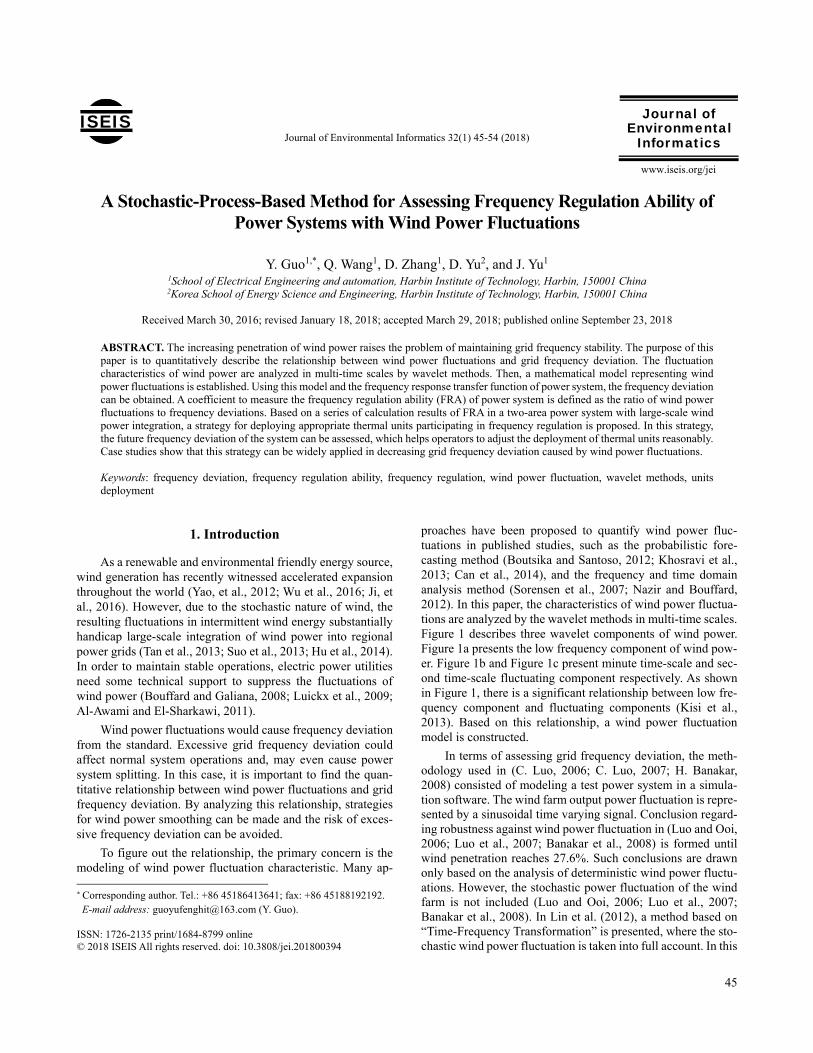
proaches have been proposed to quantify wind power fluc-tuations in published studies, such as the probabilistic fore-casting method (Boutsika and Santoso, 2012; Khosravi et al., 2013; Can et al., 2014), and the frequency and time domain analysis method (Sorensen et al., 2007; Nazir and Bouffard, 2012). In this paper, the characteristics of wind power fluctua-tions are analyzed by the wavelet methods in multi-time scales. Figure 1 describes three wavelet components of wind power. Figure 1a presents the low frequency component of wind pow-er. Figure 1b and Figure 1c present minute time-scale and sec-ond time-scale fluctuating component respectively. As shown in Figure 1, there is a significant relationship between low fre-quency component and fluctuating components (Kisi et al., 2013). Based on this relationship, a wind power fluctuation model is constructed.

In terms of assessing grid frequency deviation, the meth-odology used in (C. Luo, 2006; C. Luo, 2007; H. Banakar, 2008) consisted of modeling a test power system in a simula-tion software. The wind farm output power fluctuation is repre-sented by a sinusoidal time varying signal. Conclusion regard-ing robustness against wind power fluctuation in (Luo and Ooi, 2006; Luo et al., 2007; Banakar et al., 2008) is formed until wind penetration reaches 27.6%. Such conclusions are drawn only based on the analysis of deterministic wind power fluctu-ations. However, the stochastic power fluctuation of the wind farm is not included (Luo and Ooi, 2006; Luo et al., 2007; Banakar et al., 2008). In Lin et al. (2012), a method based on “Time-Frequency Transformation” is presented, where the sto-chastic wind power fluctuation is taken into full account. In this

* Corresponding author. Tel.: +86 45186413641; fax: +86 45188192192. E-mail address: [email protected] (Y. Guo).

ISSN: 1726-2135 print/1684-8799 online © 2018 ISEIS All rights reserved. doi: 10.3808/jei.201800394

Y. Guo et al. / Journal of Environmental Informatics 32(1) 45-54 (2018)

46

paper, a stochastic analytical approach is applied for analyzing the relationship between the stochastic wind power and grid frequency deviation. Then, a new coefficient to measure the frequency regulation ability of power system is defined.

Figure 1. Modulation effect between 15-minute moving average wind power Pw(t) and fluctuations component m(t), s(t). (a) low frequency component of wind power; (b) minute time-scale fluctuating component of wind power; (c) second time-scale fluctuating component of wind power.

To reduce the risk of excessive frequency deviation, rea-sonable power system operating strategies should be formu-lated. Many studies have shown that wind power fluctuations can be smoothed by appropriate control and deployment of conventional thermal units. The effect of fluctuating wind pow-er on frequency deviation is studied in (Sorensen et al., 2007) and operation reserve is suggested to increase with the increase of wind power scale. In (Ortega-Vazquez and Kirschen, 2009; Xia et al., 2013), methods about how to determine and deploy the system operation reserve to compensate the fluctuation of wind power are presented. In addition, system operators should dictate the dynamic requirements of the scheduled reserve ca-pacity for conducting the primary and secondary frequency regulation tasks at the system level (Galiana et al., 2005; Bouffard and Ortega-Vazquez, 2011). In general, most thermal units are participating in primary frequency regulation and only a few AGC units would participate in secondary frequency reg-ulation. In order to avoid excessive grid frequency deviation, both system operation reserve and the deployment of different kinds of thermal units should be taken into consideration. In this paper, a FRA based strategy for appropriately deploying thermal units participating in frequency regulation is proposed. Case studies are conducted to show how this strategy is im-plemented to reduce excessive frequency deviation caused by wind power fluctuations.

The main contributions of this paper are:

1) a novel multi-timescales wind power fluctuation model based on wavelet multi-resolution signal decomposition and re-construction method is proposed;

2) a method to analyze the relationship between the sto-chastic wind power and grid frequency deviation using the sto-chastic analytical approach is proposed. A new coefficient to measure the FRA of power system is defined;

3) a strategy for thermal units deployment to avoid exces-sive frequency deviation caused by wind power fluctuations is conducted.

The remainder of the paper is organized as follows. In Sec-tion 2, a time domain model of wind power fluctuation is pre-sented. The theoretical foundation and procedure for calculate-ing FRA are shown in detail in Section 3. FRA under different conditions is calculated and a strategy for deploying thermal units participating in frequency regulation is presented in Sec-tion 4. Case studies are conducted in Section 5. Conclusions are finally drawn in Section 6.

2. Modeling of the Wind Power Fluctuations

2.1. Modulation Effect of Wind Power Low Frequency Component

In this paper, the characteristic of wind power fluctuations mainly refers to the fluctuation magnitude in different time scales. The analysis is based on the actual wind power data sampled every 5-second. Measured wind power time series Pw(t) are decomposed into three parts by 8-level discrete wave-let decomposition and reconstruction methods (Rahmani, 2015). The three parts of Pw(t) are low frequency component Pw(t) , minute time-scale wind power fluctuation component Ptm(t) and second time-scale wind power fluctuation compo-nent Pts(t).

As shown in Figure 1, there is a significant relationship be-tween the low frequency component Pw(t) and the fluctuation components Pt(t) = Ptm(t) + Pts(t). The amplitude of Ptm(t) and Pts(t) are large when the amplitude of Pw(t) is large. When the amplitude of Pw(t) is nearly zero, the amplitudes of Ptm(t) and Pts(t) are also very small.

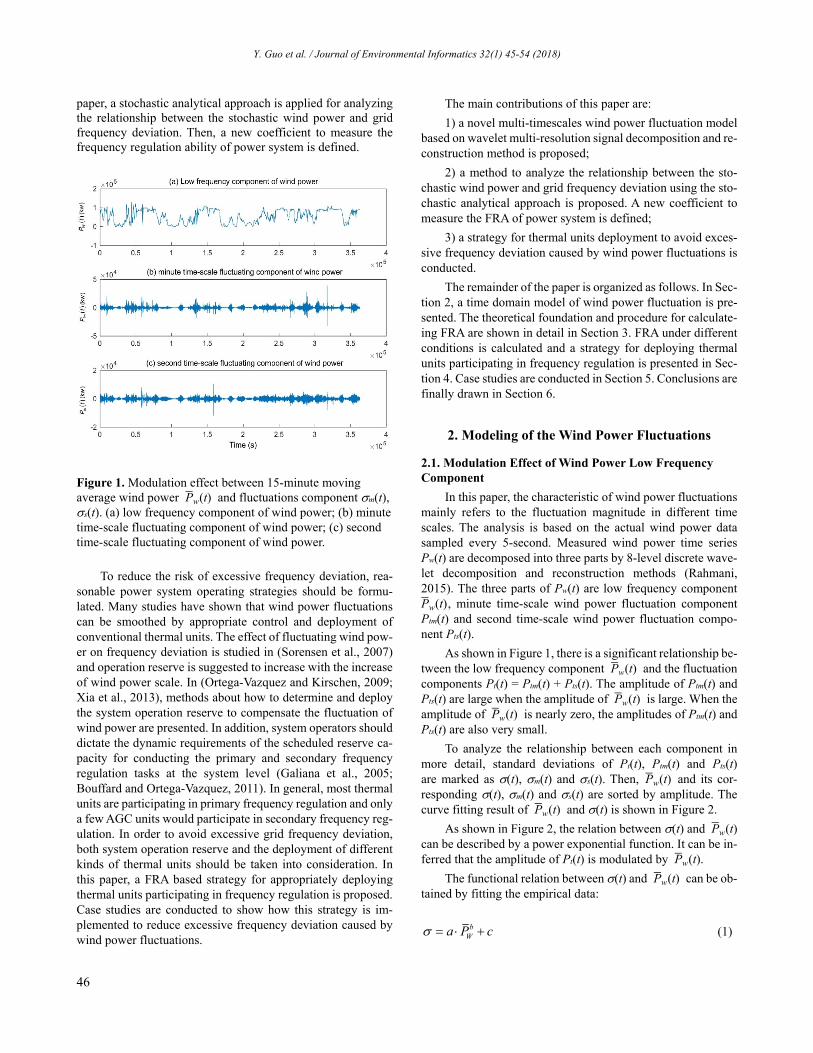
To analyze the relationship between each component in more detail, standard deviations of Pt(t), Ptm(t) and Pts(t) are marked as (t), m(t) and s(t). Then, Pw(t) and its cor-responding (t), m(t) and s(t) are sorted by amplitude. The curve fitting result of Pw(t) and (t) is shown in Figure 2.

As shown in Figure 2, the relation between (t) and Pw(t) can be described by a power exponential function. It can be in-ferred that the amplitude of Pt(t) is modulated by Pw(t).

The functional relation between (t) and Pw(t) can be ob-tained by fitting the empirical data:

b

Wa P c (1)


47

Figure 2. Fitting curve between Pw(t) and (t).

2.2. Minute-scale Wind Power Fluctuation Model

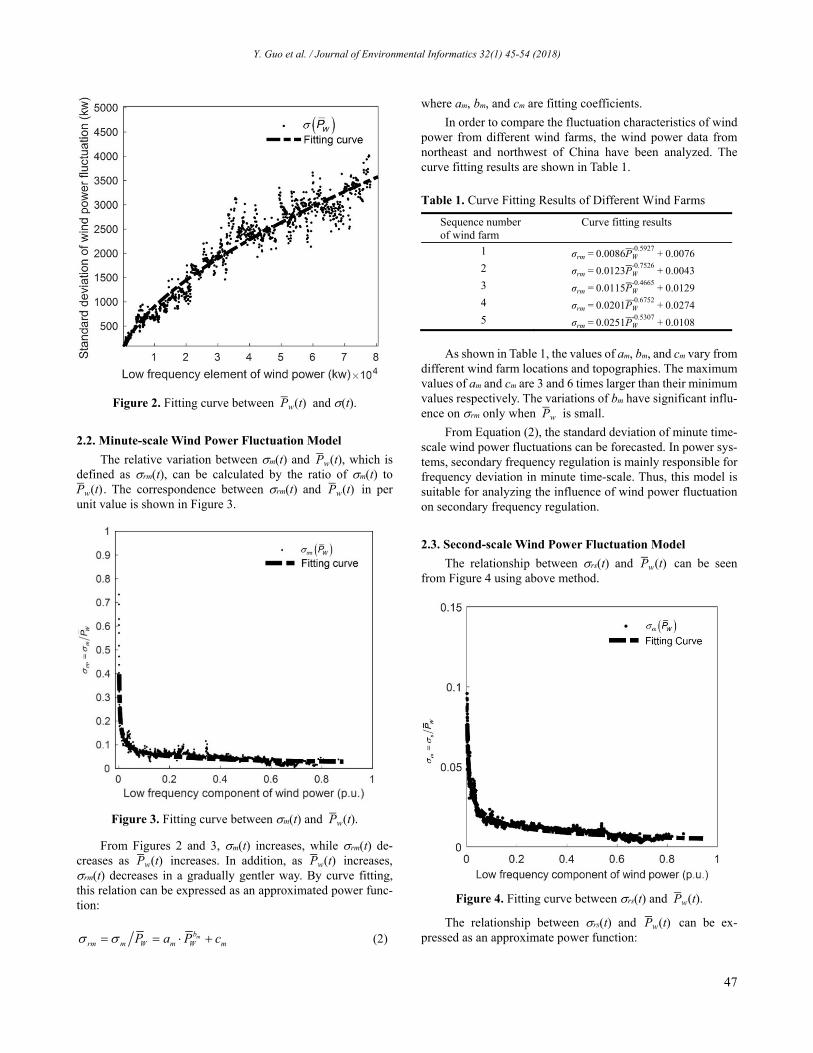
The relative variation between m(t) and Pw(t), which is defined as rm(t), can be calculated by the ratio of m(t) to Pw(t) . The correspondence between rm(t) and Pw(t) in per unit value is shown in Figure 3.

Figure 3. Fitting curve between m(t) and Pw(t).

From Figures 2 and 3, m(t) increases, while rm(t) de-creases as Pw(t) increases. In addition, as Pw(t) increases, rm(t) decreases in a gradually gentler way. By curve fitting, this relation can be expressed as an approximated power func-tion:

mb

rm m W m W mP a P c (2)

where am, bm, and cm are fitting coefficients.

In order to compare the fluctuation characteristics of wind power from different wind farms, the wind power data from northeast and northwest of China have been analyzed. The curve fitting results are shown in Table 1.

Table 1. Curve Fitting Results of Different Wind Farms

Sequence number of wind farm

Curve fitting results

1 σrm = 0.0086PW-0.5927

+ 0.0076

2 σrm = 0.0123PW-0.7526

+ 0.0043

3 σrm = 0.0115PW-0.4665

+ 0.0129

4 σrm = 0.0201PW-0.6752

+ 0.0274

5 σrm = 0.0251PW-0.5307

+ 0.0108

As shown in Table 1, the values of am, bm, and cm vary from

different wind farm locations and topographies. The maximum values of am and cm are 3 and 6 times larger than their minimum values respectively. The variations of bm have significant influ-ence on rm only when Pw is small.

From Equation (2), the standard deviation of minute time-scale wind power fluctuations can be forecasted. In power sys-tems, secondary frequency regulation is mainly responsible for frequency deviation in minute time-scale. Thus, this model is suitable for analyzing the influence of wind power fluctuation on secondary frequency regulation.

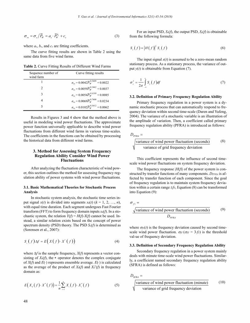
2.3. Second-scale Wind Power Fluctuation Model

The relationship between rs(t) and Pw(t) can be seen from Figure 4 using above method.

Figure 4. Fitting curve between rs(t) and Pw(t).

The relationship between rs(t) and Pw(t) can be ex-pressed as an approximate power function:


48

sb

rs s W s W sP a P c (3)

where as, bs, and cs are fitting coefficients.

The curve fitting results are shown in Table 2 using the same data from five wind farms.

Table 2. Curve Fitting Results of Different Wind Farms

Sequence number of wind farm

Curve fitting results

1 σrs = 0.0042PW-0.5409

+ 0.0022

2 σrs = 0.0059PW-0.3462

+ 0.0037

3 σrs = 0.0054PW-0.4188

+ 0.0085

4 σrs = 0.0069PW-0.7408

+ 0.0234

5 σrs = 0.0102PW-0.3612

+ 0.0062

Results in Figures 3 and 4 show that the method above is

useful in modeling wind power fluctuations. The approximate power function universally applicable to describe wind power fluctuations from different wind farms in various time-scales. The coefficients in the functions can be obtained by processing the historical data from different wind farms.

3. Method for Assessing System Frequency Regulation Ability Consider Wind Power

Fluctuations

After analyzing the fluctuation characteristic of wind pow-er, this section outlines the method for assessing frequency reg-ulation ability of power systems with wind power fluctuations.

3.1. Basic Mathematical Theories for Stochastic Process Analysis

In stochastic system analysis, the stochastic time series in-put signal x(t) is divided into segments xk(t) (k = 1, 2, …, n), with equal time duration. Each segment undergoes Fast Fourier transform (FFT) to form frequency domain inputs xk(f). In a sto-chastic system, the relation Y(f) = H(f)X(f) cannot be used. In-stead, a similar relation exists based on the concept of power spectrum density (PSD) theory. The PSD Sx(f) is determined as (Sorensen et al., 2007):

x

S f f E X f X f (4)

where f is the sample frequency, X(f) represents a vector con-sisting of Xk(f), the operator denotes the complex conjugate of X(f) and E() represents ensemble average. E() is calculated as the average of the product of Xk(f) and Xk

(f) in frequency domain as:

* *

1

1 n

k i ii

E X f X f X f X fn

(5)

For an input PSD, Sx(f), the output PSD, Sy(f) is obtainable from the following formula:

2

y xS f H f S f (6)

The input signal x(t) is assumed to be a zero-mean random

stationary process. As a stationary process, the variance of out-put y(t) is obtainable from Equation (7).

2 1

2y yS f df

(7)

3.2. Definition of Primary Frequency Regulation Ability

Primary frequency regulation in a power system is a dy-namic stochastic process that can automatically respond to fre-quency deviation within second time-scale (Daren and Yufeng, 2004). The variance of a stochastic variable is an illustration of the amplitude of variation. Then, a coefficient called primary frequency regulation ability (PFRA) is introduced as follows:

variance of wind power fluctuation (seconds)

variance of grid frequency deviation

PFRAD

(8)

This coefficient represents the influence of second time-

scale wind power fluctuations on system frequency deviation.

The frequency response |H(f)| of the power system is con-structed by transfer functions of many components. DPFRA is af-fected by transfer function of each component. Since the goal of frequency regulation is to maintain system frequency devia-tion within a certain range fT, Equation (8) can be transformed into Equation (9):

1

variance of wind power fluctuation (seconds)

f

PFRAD

(9)

where f1(t) is the frequency deviation caused by second time-scale wind power fluctuation. fT (fT = 3fT) is the threshold val-ue of frequency deviation.

3.3. Definition of Secondary Frequency Regulation Ability

Secondary frequency regulation in a power system mainly deals with minute time-scale wind power fluctuations. Similar-ly, a coefficient named secondary frequency regulation ability (SFRA) is defined as follows:

variance of wind power fluctuation (minute)

variance of grid frequency deviation

SFRAD

(10)


49

DSFRA represents the ratio of variance of minute time-scale wind power fluctuation and variance of frequency deviation during a period of time only with secondary frequency regula-tion effect. Equation (10) can be transformed into Equation (11) with the above method:

2

variance of wind power fluctuation (minute)

f

SFRAD

(11)

where f2 is the frequency deviation caused by minute time-scale wind power fluctuation.

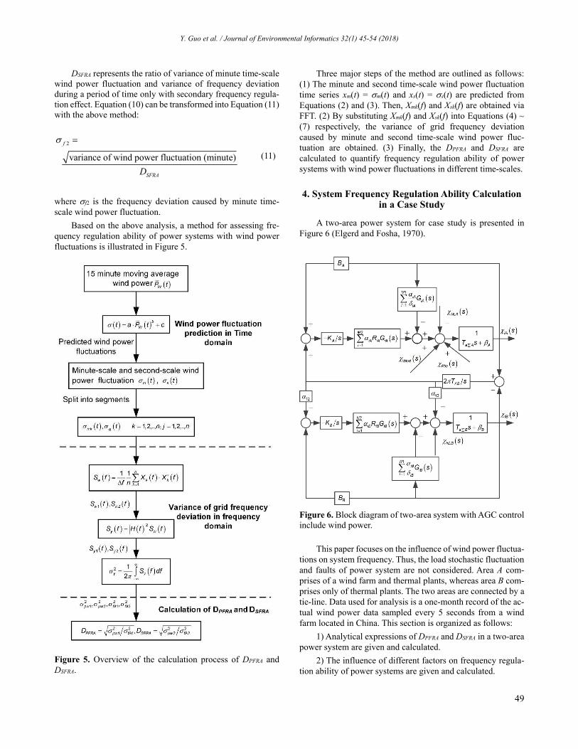
Based on the above analysis, a method for assessing fre-quency regulation ability of power systems with wind power fluctuations is illustrated in Figure 5.

Figure 5. Overview of the calculation process of DPFRA and DSFRA.

Three major steps of the method are outlined as follows: (1) The minute and second time-scale wind power fluctuation time series xm(t) = m(t) and xs(t) = s(t) are predicted from Equations (2) and (3). Then, Xmk(f) and Xsk(f) are obtained via FFT. (2) By substituting Xmk(f) and Xsk(f) into Equations (4) ~ (7) respectively, the variance of grid frequency deviation caused by minute and second time-scale wind power fluc-tuation are obtained. (3) Finally, the DPFRA and DSFRA are calculated to quantify frequency regulation ability of power systems with wind power fluctuations in different time-scales.

4. System Frequency Regulation Ability Calculation in a Case Study

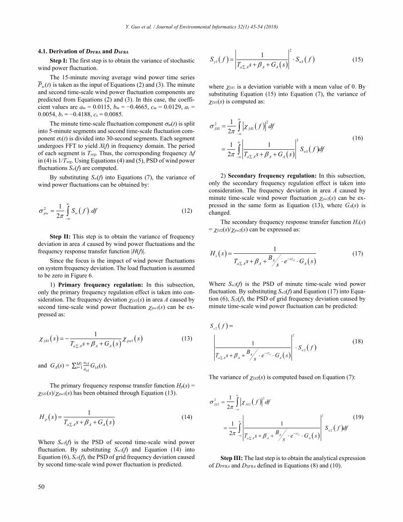
A two-area power system for case study is presented in Figure 6 (Elgerd and Fosha, 1970).

Figure 6. Block diagram of two-area system with AGC control include wind power.

This paper focuses on the influence of wind power fluctua-tions on system frequency. Thus, the load stochastic fluctuation and faults of power system are not considered. Area A com-prises of a wind farm and thermal plants, whereas area B com-prises only of thermal plants. The two areas are connected by a tie-line. Data used for analysis is a one-month record of the ac-tual wind power data sampled every 5 seconds from a wind farm located in China. This section is organized as follows:

1) Analytical expressions of DPFRA and DSFRA in a two-area power system are given and calculated.

2) The influence of different factors on frequency regula-tion ability of power systems are given and calculated.


50

4.1. Derivation of DPFRA and DSFRA

Step I: The first step is to obtain the variance of stochastic wind power fluctuation.

The 15-minute moving average wind power time series Pw(t) is taken as the input of Equations (2) and (3). The minute and second time-scale wind power fluctuation components are predicted from Equations (2) and (3). In this case, the coeffi-cient values are am = 0.0115, bm = −0.4665, cm = 0.0129, as = 0.0054, bs = −0.4188, cs = 0.0085.

The minute time-scale fluctuation component m(t) is split into 5-minute segments and second time-scale fluctuation com-ponent s(t) is divided into 30-second segments. Each segment undergoes FFT to yield X(f) in frequency domain. The period of each segment is Tseg. Thus, the corresponding frequency f in (4) is 1/Tseg. Using Equations (4) and (5), PSD of wind power fluctuations Sw(f) are computed.

By substituting Sw(f) into Equations (7), the variance of wind power fluctuations can be obtained by:

2 1

2pw wS f df

(12)

Step II: This step is to obtain the variance of frequency deviation in area A caused by wind power fluctuations and the frequency response transfer function |H(f)|.

Since the focus is the impact of wind power fluctuations on system frequency deviation. The load fluctuation is assumed to be zero in Figure 6.

1) Primary frequency regulation: In this subsection, only the primary frequency regulation effect is taken into con-sideration. The frequency deviation fA1(s) in area A caused by second time-scale wind power fluctuation pw1(s) can be ex-pressed as:

1 1

1fA pw

a A A A

s sT s G s

(13)

and GA(s) = ∑ αiA

δiAGiA(s)M1

i=1 .

The primary frequency response transfer function Hp(s) = fA1(s)/pw1(s) has been obtained through Equation (13).

1

pa A A A

H sT s G s

(14)

Where Sw1(f) is the PSD of second time-scale wind power fluctuation. By substituting Sw1(f) and Equation (14) into Equation (6), Sy1(f), the PSD of grid frequency deviation caused by second time-scale wind power fluctuation is predicted.

2

1 1

1y w

a A A A

S f S fT s G s

(15)

where fA1 is a deviation variable with a mean value of 0. By substituting Equation (15) into Equation (7), the variance of fA1(s) is computed as:

221 1

2

1

1

2

1 1

2

fA fA

wa A A A

f df

S f dfT s G s

(16)

2) Secondary frequency regulation: In this subsection, only the secondary frequency regulation effect is taken into consideration. The frequency deviation in area A caused by minute time-scale wind power fluctuation pw2(s) can be ex-pressed in the same form as Equation (13), where GA(s) is changed.

The secondary frequency response transfer function Hs(s) = fA2(s)/pw2(s) can be expressed as:

1

d

ssA

a A A A

H sBT s e G ss

(17)

Where Sw2(f) is the PSD of minute time-scale wind power fluctuation. By substituting Sw2(f) and Equation (17) into Equa-tion (6), Sy2(f), the PSD of grid frequency deviation caused by minute time-scale wind power fluctuation can be predicted:

2

2

2

1

d

y

wsA

a A A A

S f

S fB

T s e G ss

(18)

The variance of fA2(s) is computed based on Equation (7):

22

2 2

2

2

1

2

1 1

2 d

fA fA

wsA

a A A A

f df

S f dfB

T s e G ss

(19)

Step III: The last step is to obtain the analytical expression of DPFRA and DSFRA defined in Equations (8) and (10).


51

By substituting Equations (12) and (16) into Equation (8), the primary frequency regulation ability can be expressed as:

2 2

1 1

1

2

11

PFRA pw fA

w

a A A A w

D

S f df

T jf G jf S f df

(20)

where pfr and iA are the two main factors which influent the value of DPFRA.

By substituting Equations (12) and (19) into Equation (10), the secondary frequency regulation ability can be ex-pressed as:

2 2

2 2

2

2

2

1

SFRA pw fA

w

w

a A A A A A

D

S f df

S f dfT jf B K jf G jf

(21)

where GA s = ∑ αiARiAGiA(s)M2i=1 , Sw2(f) is the PSD of minute

time-scale wind power fluctuation; sfr and KA are the two main factors which influent the value of DSFRA.

4.2. Calculation of DPFRA and DSFRA of a Two-area Power System with Wind Power Fluctuations

In this section, DPFRA and DSFRA of a two-area power sys-tem are calculated. The system consists of two areas connected by a tie. Area A consists of four thermal units and a wind farm. The overall capacity of Area A and the wind farm is 3,000 and 600 MW respectively. Area B consists of four thermal units and the overall capacity is 2,000 MW. Condensation steam turbine generator is utilized in this case study. The transfer function of generator i is Gi s = 1/ T0s + a ∙1/ Tss + 1 , where Ts is the time constant for hydraulic servomotor, T0 is the time constant for high pressure cylinder volume. The values of these coeffi-cients are Ts = 0.2 s, Ts = 0.2 s, iA = iB = 0.05, KA = KB = 0.25.

(1) Calculation of DPFRA: pfr and iA are the two main factors that influent the primary frequency regulation ability. By applying the variable control method, the impacts of each factor on DPFRA are analyzed. DPFRA under different values of iA and pfr can be calculated using Matlab. The calculation re-sults are shown in Table 3.

As shown in Table 3, the DPFRA of area A increases as iA decreases or as pfr increases. Concrete analysis results are as follows:

Table 3. DPFRA at different δiA and αpfr

δiA = 0.03 δiA = 0.04 δiA = 0.05

αpfr (%) 10 20 30 40 50 60 70 80

3.3155 6.6310 9.9466 13.2621 16.5776 19.8931 23.2086 26.5242

2.4854 4.9709 7.4563 9.9418 12.4272 14.9127 17.3981 19.8836

1.9881 3.9761 5.9642 7.9523 9.9403 11.9284 13.9164 15.9045

a) DPFRA is in direct proportion to pfr when iA stays invari-ant. When the proportion of primary frequency regulation units pfr changes from p to q%. DPFRA changes from the original val-ue x to q/p ∙x.

b) When pfr has an invariant value of w, the relationship between DPFRA and iA can be described as:

PFRAiA

wD

(22)

(2) Calculation of DSFRA: Proportion of thermal units in-volved in secondary frequency regulation and KA are two main factors affect the secondary frequency regulation. The effects of each factor on DSFRA are studied using the variable control method. DSFRA under different values of sfr and KA are calcu-lated which is shown in Table 4.

Table 4. DSFRA at different KA and αsfr

KA = 0.25 KA = 0.5 KA = 0.75

αsfr (%) 10 20 30 40 50 60 70 80

5.9818 11.9636 17.9455 23.9273 29.9091 35.8909 41.8727 47.8545

15.0133 30.0267 45.0459 60.0533 75.0667 90.0800 105.0933 120.1067

23.8114 47.6227 73.4341 95.2454 119.0568 146.8642 166.6795 190.4909

From Table 4, DSFRA of area A increases as sfr increases. Concrete analysis results are as follows:

a) DSFRA is in direct proportion to sfr when KA stays invari-ant. When the proportion of primary frequency regulation units sfr changes from p to q%, DSFRA changes from the original val-ue x to q/p ∙x.

b) When sfr is invariant, DSFRA increases as KA increases. When KA increases from 0.25 to 0.5, DSFRA increases to 2.5 times of the previous value. When KA increases from 0.25 to 0.75, DSFRA increases to nearly 4 times of the previous value.

Grid operators mainly concerned about the risk of exceed-ing the frequency deviation limits due to wind power fluctua-tions for the next dispatch cycle. DPFRA and DSFRA are two prac-tical indexes to evaluate the grid’s ability of smoothing out wind power fluctuations.


52

5. Applications of DPFRA and DSFRA on Power System Operation

This section outlines how DPFRA and DSFRA are utilized in power system operation. Figure 7 illustrated the major steps of the method based on the test system of Figure 6.

Figure 7. Method of utilizing DPFRA and DSFRA on power system operation.

As shown in Figure 7, after wind power fluctuations are predicted by Equations (2) and (3), DPFRA and DSFRA can be computed by Equations (20) and (21). System frequency devia-tion due to different time-scale wind power fluctuations can be obtained from Equations (9) and (11). If the frequency devia-tions exceed the threshold values, the operator can adjust the proportion of units participating in frequency regulation in the following dispatch cycle until an acceptable frequency devia-tion is obtained.

Four case studies based on the two-area system in Figure 6 are presented:

Initial operation condition of the system: the units par-ticipating in primary frequency regulation in area A and B ac-count for 10 and 20% respectively, the units participating in secondary frequency regulation in area A and B account for 10 and 20% respectively. iA = iB = 0.05，KA = KB = 0.25. Ac-ceptable grid frequency deviation is limited to ±0.02 Hz.

Based on the method in Figure 7, four cases study are pre-sented to decrease frequency deviation. The operation condit-ions of each case are shown as follows:

Operation condition of Case I: w = 20%; pfr increases from 10 to 20%; ∑ αiA

M2i = 1 increases from 10 to 20%.

Operation condition of Case II: w = 20%; ∑ αiAM1i = 1 in-

creases from 10 to 20%; KA increases from 0.25 to 0.5.

Operation condition of Case III: w = 20%; ∑ αiAM2i = 1

increases from 10 to 20%; iA decreases from 0.05 to 0.03.

Operation condition of Case IV: w = 20%; KA increases from 0.25 to 0.5; iA decreases from 0.05 to 0.03.

Simulations are performed using MATLAB under dif-ferent operating conditions. Corresponding frequency devia-tion curves are shown in Figure 8. Figure 8a shows the frequen-cy deviation under the initial operation condition. Figure 8b ~ 8e show the frequency deviations under operation conditions of each case respectively. As seen from Figure 8a, grid fre-quency deviation cannot be maintained within a stable range of ±0.02 Hz when wind power accounts for 20% in grid.

Figure 8. Frequency deviation of Area A in different cases. (a) frequency deviation of initial condition; (b) frequency deviation of CASE I; (c) frequency deviation of CASE II; (d) frequency deviation of CASE III; (e) frequency deviation of CASE IV.

Under the operation condition of Case I, DPFRA increases from 1.9881 to 3.9761 and DSFRA increases from 5.9818 to 11.9636. Under operation condition of Case II, DPFRA increases from 1.9881 to 3.9761 and DSFRA increases from 5.9818 to


53

15.0133. Under operation condition of Case III, DPFRA in-creases from 1.9881 to 3.3155 and DSFRA increases from 5.9818 to 11.9636. Under operation condition of Case IV, DPFRA in-creases from 1.9881 to 3.3155 and DSFRA increases from 5.9818 to 15.0133.

DPFRA and DSFRA increase from the initial value in Case I ~ Case IV. The standard deviations of system frequency devia-tion under each case are shown in Figure 8. The standard devia-tion of system frequency deviation reduces from 0.00060035 to 0.00030733, 0.00029944, 0.00029641 and 0.00029335, re-spectively.

6. Conclusions

This work presents a novel method for assessing the influ-ence of stochastic wind power fluctuations on system frequen-cy deviation. This research has the following advantages:

1) Wind power fluctuation model. Stochastic wind power fluctuations are fully analyzed in multi-time scales by the wavelet methods. A power-law model with three parameters is presented. The model is available for predicting both second and minute time-scale wind power fluctuations in time domain.

2) Quantitative frequency deviation assessment. The rela-tionship between the stochastic wind power and grid frequency deviation is analyzed. Two practical indexes are defined to evaluate the grid’s ability of smoothing out wind power fluctua-tions. The evaluation results help to verify whether the perfor-mance of power system satisfies grid codes.

3) Wide adaptability. Based on the online calculation re-sults of DPFRA and DSFRA, a strategy for deploying appropriate thermal units participating in frequency regulation is presented. Cases study show that this strategy is adaptable for decreasing grid frequency deviation.

In summary, this method is particularly valuable and practical for interconnected grids with a large amount of wind power integration.

Acknowledgments. This work was supported by the Key R&D Project of China under grant number 2016YFB0901900, the National Natural Science Foundation of China (Grant No. 51676054).

Nomenclature

M1 Number of thermal units that participating in primary frequency regulation in area A.

M2 Number of thermal units that participating in second-ary frequency regulation in area A.

N1 Number of thermal units that participating in primary frequency regulation in area B.

N2 Number of thermal units that participating in second-ary frequency regulation in area B.

δiA Speed droop of generator i in area A. αiA Ratio of installed capacity of generator i to installed

capacity of area A. Ri Coefficient of power budget of the units that partici-

pating in secondary frequency regulation.

αpfr Proportion of thermal units participating in primary frequency regulation, α

pfr = ∑ αiAM1i = 1 .

αsfr Proportion of thermal units participating in secondary frequency regulation, α

pfr = ∑ αiAM1i = 1 .

Gi(s) Transfer function of generator i. Tai Time constant of rotor i, in s. TaΣ Inertia time constant of electric power system. TAB Synchronizing torque coefficient. β Coefficient of load-frequency characteristic. KA Integrator gain in AGC control of area A. BA Frequency bias factor in area A. χNL(s) Variation of system load in the frequency domain.

References

Al-Awami A.T. and El-Sharkawi M.A. (2011). Coordinated trading of wind and thermal energy. IEEE Trans. Sustainable Energy, 2(11), 277-287. https://doi.org/10.1109/TSTE.2011.2 111467

Khosravi A., Nahavandi S., and Creighton D. (2013). Prediction intervals for short-term wind farm power generation forecasts. IEEE Trans. Sustainable Energy, 4(8), 602-610. https://doi.org/10. 1109/ TSTE.2012.2232944

Luo C. and Ooi B.T. (2006). Frequency deviation of thermal power plants due to wind farms. IEEE Trans. Energy Convers.,21(12), 708-716. https://doi.org/10.1109/TEC.2006.8 74210

Luo C., Far H.G., Banakar H., and Ooi B.T. (2007). Estimation of wind penetration as limited by frequency deviation. IEEE Trans. Energy Convers., 3(6), 783-791. https://doi.org/10.1109/TEC.2006. 881082

Wu C.B., Huang G.H., Li W., Zhen J.L., and Ji L. (2016). An inexact fixed-mix fuzzy-stochastic programming model for heat supply management in wind power heating system under uncertainty. J. Cleaner Prod., 112, 1717-1728. https://doi.org/10.1016/j.jclepro. 2015.04.061

Bouffard F. and Galiana F.D. (2008). Stochastic security for operations planning with significant wind power generation. IEEE Trans. Power Syst., 23(5), 306-316. https://doi.org/10.1109/TPWRS.2008. 919318

Galiana F.D., Bouffard F., Arroyo J.M., and Restrepo J.F. (2005). Scheduling and pricing of coupled energy and primary, secondary and tertiary reserves. IEEE Proc., 93(2), 970-983. https://doi.org/ 10.1109/JPROC.2005.857492

Bouffard F. and Ortega-Vazquez M. (2011). The Value of Operational Flexibility in Power Systems with Significant Wind Power Ge-neration. Power and Energy Society General Meeting, 2011 IEEE, San Diego, CA, USA, 2011. https://doi.org/10.1109/PES.2011. 6039031

Banakar H., Luo C., and Ooi B.T. (2008). Impacts of wind power minutetominute variations on power system operation. IEEE Trans. Power Syst., 23(4), 150-160. https://doi.org/10.1109/TPWRS.2007. 913298

Lin J., Sun Y., Srensen P., and Li G. (2012). Method for Assessing Grid Frequency Deviation Due to Wind Power Fluctuation Based on TimeFrequency Transformation. IEEE Trans. Sustainable Energy, 3(2), 783-791. https://doi.org/10.1109/TST E.2011.2162639

Kisi O., Shiri J., Akbari N., Pour M.S., Hashemi A., and Tei-mourzadeh K. (2013). Modeling of dissolved oxygen in river water using artificial intelligence techniques. J. Environ. Inf., 22(2), 92-101. https://doi.org/10.3808/jei.201300248

Xia L., Junyong L., and Youbo L. (2013). Optimal Distribution Model for System Reserve Capacity with Wind Power Connection Regarding Consistency Performance of Reserve Dispatch. Autom Electric Power Syst., 40-46. https://doi.org/10.7500/AEPS201208 048


54

Ji L., Huang G.H., Huang L.C., Xie Y.L., and Niu D.X. (2016). Inexact stochastic risk-aversion optimal day-ahead dispatch model for electricity system management with wind power under uncertainty. Energy, 109, 920-932. https://doi.org/10.1016/j.energy. 2016.05. 018

Nazir Md S. and Bouffard F. (2012). Intra-hour Wind Power Cha-racteristics for Flexible Operations. Power and Energy Society General Meeting, 2012 IEEE, San Diego, CA, USA, 2012. https:// doi.org/10.1109/PESGM.2012.6345495

Ortega-Vazquez M.A. and Kirschen D.S. (2009). Estimating the spinning reserve requirements in systems with significant wind power generation penetration. IEEE Trans. Power Syst., 24(2), 114-124. https://doi.org/10.1109/TPWRS.2008.2004745

Suo M.Q., Li Y.P., Huang G.H., Deng D.L. and Li Y.F. (2013). Electric Power System Planning under Uncertainty Using Inexact Inventory Nonlinear Programming Method. J. Environ. Inf., 22(1), 49-67. https://doi.org/10.3808/jei.201300245

Elgerd O.I. and Fosha C.E. (1970). Optimum megawatt-frequency control of multiarea electric energy systems. IEEE Trans. Power Apparatus Syst., 89, 556-563. https://doi.org/10.1109/TPAS.1970. 292602

Luickx P.J., Delarue E.D., and D'Haeseleer W.D. (2009). Effect of the generation mix on wind power introduction. IET. Renewable Power Generation, 3, 267-278. https://doi.org/10.10 49/ietrpg.2008. 0061

Sorensen P., Cutululis N.A., and Vigueras-Rodrigue A. (2007). Power fluctuations from large wind farms. IEEE Trans. Power Syst., 22, 958-965. https://doi.org/10.1109/TPWRS.2007. 901615

Hu Q., Huang G. H., Cai Y. P., and Sun W. (2014). Planning of Electric Power Generation Systems under Multiple Un-certainties and Constraint -Violation Levels. J. Environ. Inf., 23(1), 55-64. https:// doi.org/10.3808/jei.201400257

Rahmani, M.A. (2015). The use of statistical weather generator, hybrid data driven and system dynamics models for water resources management under climate change. J. Environ. Inf., 25(1), 23-35. https://doi.org/10.3808/jei.201400285

Boutsika T. and Santoso S. (2012). Quantifying short-term wind power variability using the conditional range metric. IEEE Trans. Sustainable Energy, 3, 369-378. https://doi.org/10.1109/TSTE.2012. 2186617

Can W., Xu Z., Pinson P., Dong Z.Y., and Kit Po.W. (2014). Pro-babilistic Forecasting of Wind Power Generation Using Extreme Learning Machine. IEEE Trans. Power Syst., vol. 29, 1033-1044. https://doi.org/10.1109/TPWRS.2013.2287871

Daren Y. and Guo Y.F. (2004). The online estimate of primary frequency control ability in electric power system. CSEE Proc., 24, 72-76.

Yao Y., Huang G.H., and Lin Q.G. (2012). Climate change impacts on Ontario wind power resource. Environ. Syst. Res., 1(1). https://doi. org/2.10.1186/2193-2697-1-2

Tan Z.F., Sog Y.H., Shen Y.S., Zhang C., and Wang S. (2013). An Optimization-Based Study to Analyze the Impacts of Clean Energy and Carbon Emission Mechanisms on Inter-Regional Energy Exchange. J. Environ. Inf., 22(2), 123-130. https://doi.org/10.3808/ jei.201300251

a stochastic-process-based method for assessing frequency...

Documents