A Stochastic Model for Predicting the Probability Distribution of the Dissolved-Oxygen Deficit in Streams

GEOLOGICAL SURVEY PROFESSIONAL PAPER 913

A Stochastic Model for Predicting the Probability Distribution of the Dissolved-Oxygen Deficit in Streams

By I. I. ESEN and R. E. RATHBUN

GEOLOGICAL SURVEY PROFESSIONAL PAPER 913

A description of the development and application of

a stochastic model for predicting the probability

distribution of the dissolved-oxygen deficit at

points in a stream downstream from a waste source

UNITED STATES GOVERNMENT PRINTING OFFICE, WASHINGTON 1976

UNITED STATES DEPARTMENT OF THE INTERIOR

THOMAS S. KLEPPE, Secretary

GEOLOGICAL SURVEY

V. E. McKelvey, Director

Library of Congress Cataloging in Publication Data Esen, I. I. A stochastic model for predicting the probability distribution of the dissolved-oxygen deficit in streams. (Geological Survey professional paper ; 913) Bibliography: p. Supt. of Docs. no.: I 19.16:913

1. Water-Dissolved oxygen-Mathematical models. 2. Biochemical oxygen demand-Mathematical models. 3. Random walks (Mathematics) I. Rathbun, R. E., joint author. II. Title: A stochastic model for predicting the probability distribution . . . III. Series: United States. Geological Survey. Professional paper ; 913.

TD737.E78 551.4'83 74-31208

For sale by the Superintendent of Documents, U.S. Government Printing Office Washington, D.C. 20402

Stock Number 024-001-02808-5

CONTENTS

Page

Symbols ----------------------------------------- iv Metric-English equivalents ------------------------ viii

~bstract ----------------------------------------- 1 Introduction ___ _ _ _ _ __ _ ___ _ ___ _ _ __ _ _ ___ ___ __ __ _ _ _ _ _ 1

~ckno~ledgrnents --------------------------------- 3 Variations in the deoxygenation and reaeration

coefficients --------------------------------- 4 Deoxygenation coefficient, K1 ------------------- 4 Reaeration coefficient, K2 ---------------------- 5 Correlation betw'een deoxygenation and reaeration

coefficients --------------------------------- 6 Development of the probabilistic model -------------- 7

Solution of equations for longitudinal profiles of BOD and dissolved-oxygen concentration____ 7

Random walk models -------------------------- 8 Deoxygenation coefficient, K1 --------------- 8 Reaeration coefficient, K2 ------------------ 9

Monte Carlo simulation technique for dissolved-oxygen deficit ------------------------------ 9

~pplication of the technique and discussion of

results ------------------------------------- 11

Development of the probabilistic model--Continued ~pplication of the technique and discussion

of results-Continued

Paee

Hypothetical example ---------------------- 11 Sacramento River data -------------------- 15

Estimation of the accuracy of the Monte Carlo

procedure ---------------------------------- 17 Estimation of the variance of the oxygen-deficit

distribution --------------------------------- 19 Extension of the model --------------------------- 22

Monte Carlo computations --------------------- 24 Estimation of the mean and the variance of the

oxy~n-deficit distribution -------------------- 24 Estimation of a stochastic critical time of traveL_ 26 Presentation and discussion of results ---------- 26

Critical time of travel --------------------- 26 Mean oxygen deficit ----------------------- 27 Variance of the oxygen deficit -------------- 29

Evaluation of the model --------------------------- 36 Summary ---------------------------------------- 38 Literature cited ----------------------------------- 40 Supplemental data -------------------------------- 42

ILLUSTRATIONS

Paee FIGURES 1-21. Graphs showing:

1. Distribution of the oxygen deficit estimated for the conditions of .case 1 ----------------- 13 2. Distribution of the oxygen deficit estimated for the conditions of ··case 2 ----------------- 13 3. Distribution of the oxygen deficit estimated for the conditions of ease 3 ---------------- 14 4. Mean oxygen deficit and 10 and 20 percentile limits as a function of time for the oxygen-

deficit distributions estimated for the conditions of cases 1, 2, and 3 ----------------- 15 5. Experimental dissolved-oxygen concentrations, mean dissolved-oxygen concentrations pre­

dicted by the deterministic model ( eq 39) , and mean, 10 and 20 percentile limits of the dissolved-oxygen concentrations predicted by the stochastic model ( eq 41) ; Sacra-mento River data ------------------------------------------------------------- 16

6. Distribution of the oxygen deficit as estimated from equation 41; Sacramento River data 17 7. Observed and predicted variance of the oxygen-deficit distributions as a function of time,

Sacramento River data --------------------------------------------------------- 18 8. 'lr-parameter as a function of the reaeration and deoxygenation coefficients; time of travel

of 1 day ------------~--------------------------------------------------------- 21 9. 'lr-parameter as a function of the reaeration and deoxygenation coefficients; time of travel

of 2 days -------------------------------------------------------------------- 22 10. 'lr-parameter as a function uf the reaeration and deoxygenation coefficients; time of travel of

3 days ----------------------------------------------------------------------- 23 11. Critical time of travel (deterministic model) as a function of the deoxygenation and reaera-

tion coefficients --------------------------------------------------------------- 27 12. Critical time of travel (stochastic model) as a function of the deoxygenation and reaeration

coefficients -------------------------------------------------------------------- 28 13. Percentage difference in deterministic and stochastic critical times of travel as a function of

the ratio of the reaeration and deoxygenation coefficients -------------------------- 29

Ill

IV CONTENTS

FIGURES 1-21. Graphs showing-Continued Page

14. Oxygen deficit as a function of the ratio of the reaeration and deoxygenation coefficients; deterministic and stochastic models ---------------------------------------------- 30

15. Oxygen deficit as a function of the ratio of the reaaration and deoxygenation coefficients; stochastic model and Taylor series approximation -------------------------------- 30

16. Variance of the oxygen deficit as a function of the ratio of the reaeration and deoxygena-tion coefficients; stochastic model and Taylor series approximation with the determi-nistic critical time of travel ---------------------------------------------------- 31

17. Variance of the oxygen deficit as a function of the ratio of the reaeration and deoxygenation coefficients; stochastic model and Taylor series approximation with the stochastic cri-tical time of travel ------------------------------------------------------------ 32

18. Variance of the oxygen deficit as a function of the ratio of the reaeration and deoxygenation coefficients; stochastic model with the deterministic and stochastic critical times of

travel ------------------------------------------------------------------------ 33 19. Variance of the oxygen deficit as a function of the ratio of the reaeration and deoxygena-

tion coefficients; Taylor series approximation with the deterministic and stochastic criti-cal times of travel ------------------------------------------------------------- 34

20. Distribution of the variance among the terms making up the variance as a function of the ratio of the reaeration and deoxygenation coefficients ----------------------------- 35

21. Variance of the oxygen deficit as a function of the deoxygenation and reaeration ooefficients; stochastic model with the stochastic critical times of travel ------------------------ 36

22. Flow chart for the computer program for the stochastic model for estimating the variance of the

oxygen deficU -------------------------------------------------------------------------- 48 23. Continuation of the flow chart for the computer program for the stochastic model for estimating the

variance of the oxygen deficit ------------------------------------------------------------ 49 24. Completion of the flow chart for the computer program for the stochastic model for estimating the

variance of the oxygen deficit ------------------------------------------------------------ 50

TABLES

Paee TABLE 1. Dissolved-oxygen deficit from equation 4 and significant parameters of the stochastic oxygen-deficit

distribution ----------------------------------------------------------------------------- 12 2. Correlation coefficients between BOD and oxygen deficit ----------------------------------------- 14 3. Significant parameters of the oxygen-deficit distribution for the Sacramento River data ----------- 16 4. Variance of the oxygen-deficit distributions determined from the stochastic model and the Taylor series

approximation (eq 65) ------------------------------------------------------------------ 22 5. Critical time of travel for the deterministic and stochastic models and percentage difference -------- 26 6. Mean oxygen deficit for deterministic and stochastic models -------------------------------------- 28 7. Mean oxygen deficit for stochastic model and Taylor series approximation; with Tc

8 ------------- 29

8. Variance of the oxygen deficit from the stochastic model and the Taylor series approximation ------- 29 9. Distribution of the variance among the terms making up the variance estimated by the Taylor series

approximation of the stochastic model ---------- ------------------------------------------- 35 10. Biochemical-oxygen-demand data for the Ohio River (from Kothandaraman, 1968) and results of the

data analysis --------------------------------------------------------------------------- 43 11. Mean, variance, and coefficient of variation of the reaeration coefficient data of Churchill, Elmore, and

Buckingham (1962) --------------------------------------------------------------------- 45 12. Correlation coefficient between the biochemical-oxygen-demand and the dissolved-oxygen concentration

(from Moushegian and Krutchkoff, 1969) -------------------------------------------------- 46 13. Dissolved-oxygen concentration data for the Sacramento River (from Thayer and Krutchkoff, 1966) -- 47

SYMBOLS

Symbol Definition Symbol Definition a ___________________ Parameter equal to K2-K1-Ka, in re-

ciprocal days. B ___________________ Assumed deterministic part of the dis-

solved-oxygen deficit, defined by equation 40, in milligrams per litre.

BOD ________________ Biochemical-oxygen-demand, in milli-

grams per litre.

C ___________________ Dissolved-oxygen concentration, in mil-

ligrams per litre.

CONTENTS v

Symbol Definition

C. ------------------Rate of addition of dissolved oxygen along the reach by all processes other than reaeration and photosyn­thesis, in milligrams per litre per day.

C" CJ-1 --------------Dissolved-oxygen concentration at the end of the time of travel T1 and TJ-1, respectively, in milligrams per litre.

Co ------------------Dissolved-oxygen concentration at the upstream end of the reach, in milli­grams per litre.

C. __________________ Dissolved- oxygen concentration at saturation, in milligrams per litre.

C., (Z) _______________ Coefficient of variation of the random variable Z.

D __________________ Dissolved-oxygen deficit, or the differ-ence between the dissolved-oxygen concentration at saturation and the actual dissolved-oxygen concentra­tion.

DB ------------------Rate of removal of dissolved oxygen by the benthal layer on the stream bottom, in milligrams per litre per day.

Dt __________________ Dissolved-oxygen deficit for the kth iteration of the Monte Carlo simula­tion procedure, in milligrams per litre.

Do ------------------Dissolved-oxygen deficit at the up­stream end of the reach, in milli­grams per litre.

Dz ------------------Longitudinal dispersion coefficient, in square feet per day.

E ------------------Error in the fourth central moment of K1T, defined by equation 51.

E (Z) ---------------Expected value of the random variable z.

/(0 ----------------Function describing the variation with time ~ of the BOD at the upstream end of the reach, in milligrams per litre.

/L ( ·) ---------------Probability density function of the BOD, defined by equation 32.

F(n ----------------Function describing the variation with time ~ of the dissolved-oxygen con­centration at the upstream end of the reach, in milligrams per litre.

g -------------------Function of the deoxygenation and re­aeration coefficients that gives the random part of the dissolved-oxygen deficit, defined by equation 54, in milligrams per litre.

G1 ------------------Term giving the effect on the mean dissolved-oxygen deficit of random variations in the deoxygenation co­efficient, defined by equation 59, in milligrams per litre.

G2 __________________ Term giving the effect on the mean dissolved-oxygen deficit of random variations in the reaeration coeffi­cient, defined by equation 60, in mil­ligrams per litre.

Symbol Definition

Ga ------------------Term givmg the effect on the mean dissolved-oxygen deficit of correla­tion between the deoxygenation and reaeration coefficients, defined by equation 61, in milligrams per litre.

G~ ------------------Term giving the effect on the variance of the dissolved-oxygen deficit of random variations in the deoxygena­tion coefficient, defined by equation 66, in (milligrams per litre) squared.

Gs ------------------Term giving the effect on the variance of the dissolved-oxygen deficit of random variations in the reaeration coefficient, defined by equation 67, in (milligrams per litre) squared.

Ge ------------------Term giving the effect on the variance of the dissolved-oxygen deficit of correlation between the deoxygena­tion and reaeration coefficients, de­fined by equation 68, in (milligrams per litre) squared.

k -------------------Function of the deoxygenation coeffi­cient at the upstream end of the reach, the deoxygenation coefficient along the reach, the reaeration coeffi­cient, and the BOD at the upstream end of the reach that gives the random part of the dis,solved-oxygen deficit, defined by equation 72, in milligrams per litre.

H __________________ Mean depth of flow, in feet.

H1 ------------------Term giving the effect on the mean dissolved-oxygen deficit of random variations in the deoxygenation co­efficient along the reach, defined by equation 76, in milligrams per litre.

H2 ------------------Term giving the effect on the mean dissolved-oxygen deficit of random variations in the reaeration coeffi­cient, defined by equation 77, in milligrams per litre.

Hs ------------------Term giving the effect on the mean dissolved-oxygen deficit of correla­tion between the deoxygenation co­efficient along the reach and the re­aeration coefficient, defined by equa­tion 78, in milligrams per litre.

H, ------------------Term giving the effect on the mean dissolved-oxygen deficit of random variations in the deoxygenation co­efficient at the upstream end of the reach, defined by equation 79, in milligrams per litre.

Hs ------------------Term giving the effect on the mean dissolved-oxygen deficit of correla­tion between the BOD and the de­oxygenation coefficient at the up­stream end of the reach, defined by equation 80, in milligrams per litre.

VI CONTENTS

Symbol Definition

Ho ------------------Term giving the effect on the variance of the dissolved-oxygen deficit of. random variations in the deoxygena­tion coefficient along the reach, de­fined by equation 84, in (milligrams per litre) squared.

H1 ------------------Term giving the effect on the variance of the dissolved-oxygen deficit of random variations in the Teaeration coefficient, defined by equation 85, in (milligrams per litre) squared.

Hs ------------------T-erm giving the effect on the variance of the dissolved-oxygen deficit of correlation between the deoxygena­tion coefficient along the reach and the reaeration coefficient, defined by equation 86, in (milligrams per litre) squared.

Hu ------------------Term giving the effect on the vari­ance of the dissolved-oxygen deficit of random variations in the BOD at the upstream end of the reach, defined by equation 87, in (milli­grams per litre) squared.

Hto -----------------Term giving the effect on the variance of the dissolved-oxygen deficit of random variations in the deoxygena­tion, coefficient at the upstream end of the reach, defined by equation 88, in (milligrams per litre) squared.

Hu -----------------Term giving the effect on the variance of the dissolved-oxygen deficit of correlation between the BOD and the deoxygenation coefficient at the upstream end of the reach, defined by equation 89, in (milligrams per litre) squared.

i ____________________ DenotetS a summation index.

l -------------------Term giving the effect of the addition of BOD along the reach, defined by equation 27, in milligrams per litre.

i ___________________ Denotes a ·summation index.

k -------------------Deoxygenation coefficient along the ,zoeach or the rate constant for the biochemical oxidation of carbona­ceous material along the reach; as­sumed to be a function of the dis­tance downstream ( x) or equiva­lently of time of travel (.T), in re­ciprocal days.

k,, k,+t, klt kn ________ Deoxygenation coefficient along the reach after i, i+1, j, and n steps, respectively, of the random walk process, in reciprocal days.

k -------------------Mean value of the deoxygenation co­efficient along the reach, in recipro­cal days..

Symbol Definition Kt __________________ Deoxygenation coefficient or the rate

constant for the biochemical oxida­tion of carbonaceous material; as­sumed to be a function of the dis­tance downstream (,x) , or equiva­lently of the time of travel ( T) , in reciprocal days.

Kt1

_________________ Initial value of the deoxygenation co-efficient or the deoxygenation coeffi­cient at the upstream end of the reach, in reciprocal days.

K1i, Kli+l' K1p K1n ---Deoxygenation coefficient after i, i+1, j, and n steps, respectively of the random walk process; equivalently, Kti is the deoxygenation coefficient at the end of time of travel T,, in reciprocal days.

Kt __________________ Mean value of the deoxygenation co-efficient, in reciprocal days.

Kt(T) ______________ Mean value of the deoxygenation co-efficient at any time of travel T, in reciprocal days.

K2 __________________ Reaeration coefficient or the rate con-stant for oxygen absorption from the atmosphere, in reciprocal days.

Kzi, Kzi+l' Kzi, Kzn----Reaeration coefficient after i, i+1, j, and ,n steps, respectively, of the random walk process; equivalently, K2i is the reaeration coefficient at the end of time of travel T" in re­ciprocal days.

K2 __________________ Mean value of the reaeration coeffi-cient, in reciprocal days.

K2( T) ______________ Mean value of the reaeration coeffi-cient at any time of travel T, in re­ciprocal days.

K220

________________ Reaeration coefficient at 20° Celsius, in reciprocal days.

K2P -----------------Reaeration coefficient predicted by equation 15, in reciprocal days.

Ka ------------------Rate constant for the removal of BOD by sedimentation and adsorption, in reciprocal days.

L __________________ BOD or biochemical-oxygen-demand of carbonaceous material, in milli­grams per litre.

L" L;-1 --------------BOD a,t the end of times of travel of T, and T;-t, respectively, in milli­grams per litre.

L ___________________ Mean value of the BOD, in milli-grrams per litre, defined by equation 33.

La ------------------Rate of addition of BOD along the reach, in milligrams per litre per day.

Lo __________________ BOD at the upstream end of the

reach, in milligrams per litre. Lo1, Lo2 , ••• Lon ______ BOD at the upstream end of the reach

at the end of 1, 2, ... n steps of the random walk process, in milligrrams peT litre.

CONTENTS VII

Symbol Definititm

Lo ------------------Mean value of the BOD at the up­stream end of the reach, in m'illi­grams per litre.

m -------------------Number of times that the Monte Carlo simulation procedure is repeated.

n ___________________ Number of steps in the random walk process.

P -------------------Rate of production of dissolved oxygen by photosynthesis, in milligrams per litre per day.

'PI or Pt(Ll.Kt) ________ Probability that K1 takes a positive step in the random walk process.

'P2 or P:~(L1K2) ________ Probability that K2 takes a positive step in the random walk process.

P[Z=y] -------------Probability that the outcome of the event Z is y.

q1 or q1 (Ll.Kt) --------Probability that K1 takes a negative step in the random walk process.

q2 or q2(Ll.K2) ________ Probabil'ity that K2 takes a negative step in the random walk process.

rp ------------------Rate of consumption of dissolved oxygen by plant respiration, in mil­ligrams per litre per day.

r(Zt, Z2) ____________ Correlation coefficient between the random variables Z1 and Z2.

r(BOD, C) __________ Correlation coefficient between the BOD and the dissolved-oxygen con­centration.

r(BOD, D) ----------Correlation coefficient between the BOD and the dissolved-oxygen deficit.

R1i -----------------Set of n uniformly distributed random numbel'IS used in the Monte Carlo simulation of random variations in the deoxygenation coefficient.

R2i _________________ Set of n uniformly distributed random numbe:rs used in the Monte Carlo simulation of random variations in the reaeration coefficient.

t -------------------Time, in days.

J:r dx T ------------------Time of travel or -; subscripts j

0 v and j-1 indicate specific times of travel, in days.

Tc ------------------Critical time of travel o~ the time at which the dissolved-oxygen deficit is maximum, in days.

Ten -----------------Critical ttime of ·travel for the deter­ministic model ( eq 4) , in daY15.

Tc8 -----------------Critical time of travel estimated from the Taylor series approximation of the stochastic model ( eq 7 4) , in days.

Var (Z) ------------Variance of the random variable Z.

V ------------------Mean velocity of flow, in feet per second or equivalent.

x -------------------Longitudinal position or distance downstream, in feet.

X ------------------Amount of BOD removed or the amount of dissolved oxygen con­sumed, in milligrams per litre.

Symbol Definititm

Xh XJ-t -------------Amounts of BOD removed at the end of times of travel T1 and TJ-t, re­spectively; in milligrams per litre.

Z ------------------Random variable. Zm __________________ Mean value of a random sample of

size m. al ___________________ Drift coefficient for the deoxygenation

coefficient, defined by equation 30. a2 -------------------Drift coefficient for the reaeration co­

efficient, defined by equation 37. f3t ------------------Variance of the total deoxygenation

coefficient (Kt+k), in (reciprocal days) squared.

fJ't ------------------Variance of the deoxygenation coeffi­cient at the upstream end of the reach, in (reciprocal days) squared.

f3''t -----------------Variance of the deoxygenation coeffi­cient along the reach, in (reciprocal days) squared.

fJ2 ------------------Varriance of the reaeration coefficient, in (reciprocal days) squared.

a ___________________ confidence limit.

L1 -------------------Parameter of the stochastic model of Thayer and Krutchkoff (1966) for estimating the distribution of the biochemical-oxygen-demand and the dissolved-oxygen deficit, in milli­grams per litre.

L1K1 _________________ Step length of the random walk for the deoxygenation coefficient, com­puted from equation 31.

L1K2 -----------------Step length rof the random walk for the rea.eration coefficient, computed from equation 38.

Ll.T -----------------Incremental value of the time of travel, equal to TIn; in days.

£ -------------------Expected deviation from the mean value of the random variable Z.

p, ___________________ Mean value.

P,4(j) ________________ Fourth moment of a binomial distribu-tion.

P.4(KtT, N) _________ Fourth central moment of the limit-ing normal distribution of K1T, in reciprocal days to the fourth power.

P,4(KtT, Ll.T) ----------Fourth central moment of the scaled binomial distribution describing K1T for finite Ll.T, in reciprocal days to the fourth power.

!"' dx r -------------------t- -or t-T, in days.

0 v 'lT -------------------The constant 3.14. a -------------------Standard deviation.

q2 -------------------Variance. ,., ,., _________________ Dummy variables of integration. v ___________________ Function of the deoxygenation and

reaeration coefficients and the time of travel for estimating the variance of the dissolved-oxygen deficit, de­fined by equation 69.

VIII

Metric unit

millimetre (mm) metre (m) kilometre (km)

square metre (m2) square kilometre (km2) hectare (ha)

cubic centimetre (cm3) litre (I) cubic metre (m3) cubic metre cubic hectometre (hm3) litre litre litre cubic metre

cubic metre

gram (g) gram tonne (t) tonne

CONTENTS

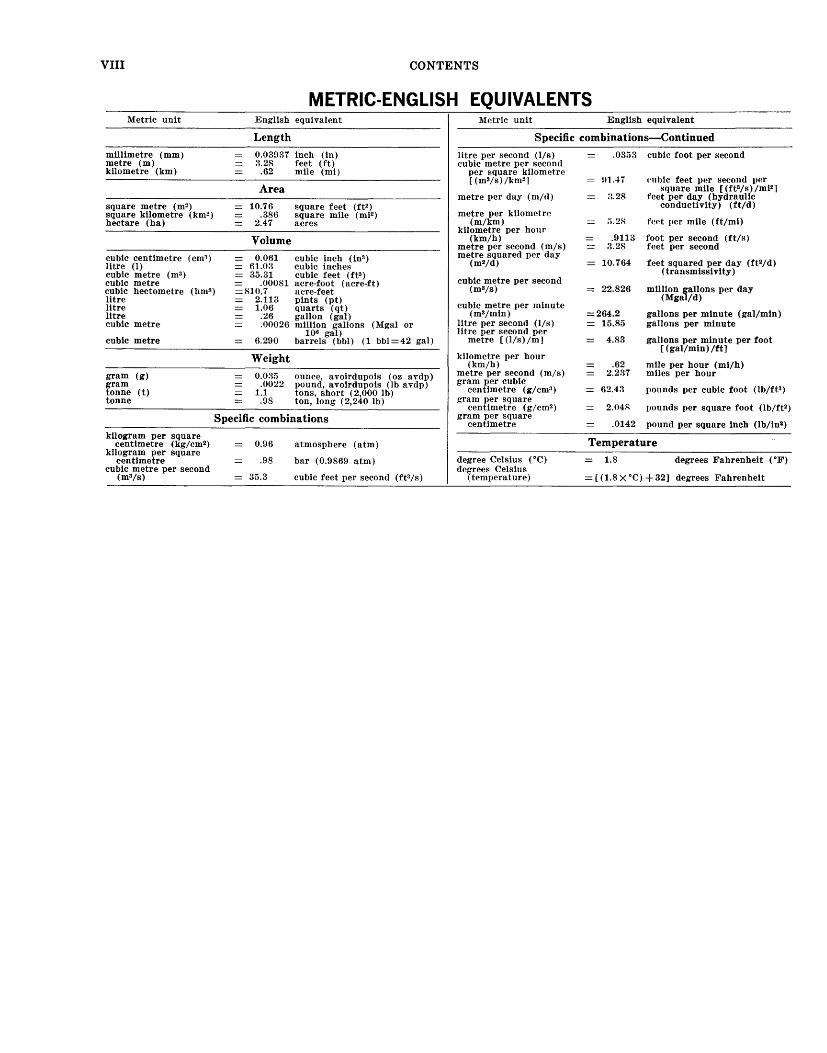
METRIC-ENGLISH EQUIVALENTS English equivalent

Length

0.03937 inch (in) 3.28 feet (ft)

.62 mile (mi)

Area

10.76 .386

2.47

Volume

0.061 61.0?. 35.31

.00081 =810.7

2.113 1.06

.26

.00026

6.290

Weight

0.035 .0022

1.1 .98

square feet (ft2) square mile (mi2) acres

cubic inch (in3) cubic inches cubic feet (ft3) acre-foot (acre-ft) acre-feet pints (pt) quarts (qt) gallon (gal) million gallons (Mgal or

106 gal) barrels (bbl) (1 bbl=42 gal)

ounce, avoirdupois (oz avdp} pound, avoirdupois (lb avdp) tons, short ( 2,000 lb) ton, long ( 2,240 lb)

Metric unit English equivalent

Specific combinations-Continued

litre per second (1/s} .0353 cubic foot per second cubic metre per second

per square kilometre [ (m3/s)/km2]

metre per day (m/<1)

metre per kilometre (m/km)

kilometre per hour (km/h)

metre per second (m/s) metre squared per day

(m2jd)

cubic metre per second (mSjs)

cubic metre per minute (mSjmin)

litre per second (1/s) litre per second per

metre [(1/s)/m]

kilometre per hour (km/h)

metre per second (m/s) gram per cubic

centimetre (g/cm3 )

gram per square centimetre (g/cm2 )

!11.47

::.28

:i.2S

.9113 :::.28

10.764

= 22.826

=264.2 15.85

4.83

.62 2.237

62.43

2.048

I'Hhic feet per second per square mile [ (fta/s) /mi2]

feet per day (hydraulic conductivity) (ft/d)

fe•~t per mile (ft/mi)

foot per second (ft/s) feet per second

feet squared per day (ft2/d) (transmissivity)

million gallons per day (Mgal/d)

gallons per minute (gal/min) gallons per minute

gallons per minute per foot [(gal/min) /ft]

mile per hour (mi/h) miles per hour

Specific combinations gram per square centimetre .0142

pounds per cubic foot (lb/ft3 )

pounds per square foot (lb/ft2)

pound per square inch (lb/in2) kilogram per square

centimetre (kg/cm2) kilogram per square

centimetre cubic metre per second

(ms;s}

0.96

.98

35.3

atmosphere (atm)

bar (0.9869 atm)

cubic feet per second (fts;s)

degree Celsius (°C) degrees Celsius

(temperature)

Temperature

1.8 degrees Fahrenheit (°F)

= [ ( 1.8 X °C) + 32] degrees Fahrenheit

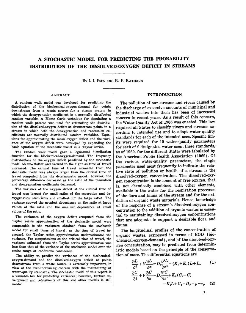
A STOCHASTIC MODEL FOR PREDICTING THE PROBABILITY

DISTRIBUTION OF THE DISSOLVED-OXYGEN DEFICIT IN STREAMS

By I. I. EsEN and R. E. RATHBUN

ABSTRACT

A random walk model was developed for predicting the distribution of the biochemical-oxygen-demand for points downstream from a waste source for a stream system in which the deoxygenation coefficient is a normally distributed random variable. A Monte Carlo technique for simulating a random walk process was used for estimating the distribu­tion of the dissolved-oxygen deficit at downstream points in a stream in which both the deoxygenation and reaeration co­efficients are normally distributed random variable:s. Equa­tions for approximating the mean oxygen deficit and the vari­ance of the oxygen deficit were developed by expanding the basic equation of the stochastic model in a Taylor series.

The random walk model gave a lognormal distribution function for the biochemical-oxygen-demand. The frequency distributions of the oxygen deficit predicted by the stochastic model became flatter and skewed to the right as time of travel increased. The critical time of travel estimated from the stochastic model was always larger than the critical time of travel computed from the deterministic model; however, the percentage difference decreased as the ratio of the reaeration and deoxygenation coefficients decreased.

The variance of the oxygen deficit at the critical time of travel was largest for small ratios of the reaeration and de­oxygenation coefficients and smallest for the lall'ge ratios. The variance showed the greatest dependence on the ratio at large values of the ratio and the smallest dependence at small values of the ratio.

The variances of the oxygen deficit computed from the Taylor series approximation of the stochastic model were comparable to the variances obtained from the stochastic model for small times of travel; as the time of travel in­creased, the Taylor series approximation underestimated the variance. For computations at the critical time of travel, the variance estimated from the Taylor series approximation was less than that of the variance of the stochastic model over the entire range of conditions considered.

The ability to predict the variances of the biochemical­oxygen-demand and the dissolved-oxygen deficit at points downstream from a waste source is extremely important, in view of the ever-increasing concern with the maintaining of water-quality standards. The stochastic model of this report is a valuable tool for predicting variances ; however, further de­velopment and refinements of this and other models is still needed.

INTRODUCTION

The pollution of our streams and rivers caused by the discharge of excessive amounts of municipal and industrial wastes into them has been of increased concern in recent years. As a result of this concern, the Water Quality Act of 1965 was enacted. This law required all States to classify rivers and streams ac­cording to intended use and to adopt water-quality standards for each of the intended uses. Specific lim­its were required for 10 water-quality parameters for each of 9 designated water uses; these standards, as of 1969, for the different States were tabulated by the American Public Health Association ( 1969) . Of the various water-quality parameters, the single parameter used most frequently to indicate the rela­tive state of pollution or health of a stream is the dissolved-oxygen concentration. The dissolved-oxy­gen concentration is the amount of free oxygen, that is, not chemically combined with other elements, available in the water for the respiration processes of the flora and fauna of the stream and for the oxi­dation of organic waste materials. Hence, knowledge of the response of a stream's dissolved-oxygen con­centration to the addition of organic wastes is essen­tial to maintaining dissolved-oxygen concentrations that are adequate to support a desirable flora and fauna.

The longitudinal profiles of the concentration of organic wastes, expressed in terms of BOD (bio­chemical-oxygen-demand), and of the dissolved-oxy­gen concentration, may be predicted from determin­istic models based on the principle of the conserva­tion of mass. The differential equations are

oL oL o2L -+ V-=Dm-- (Kt+Ks)L+La ()t ()X ()X2

(1)

oC oC o 2C -+ V-=Dm-+K2(Cs-C) ()t ()X ()X 2

-KtL+Ca-DB+p-rp (2)

1

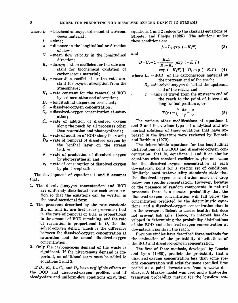
2 MODEL FOR PREDICTING THE DISSOLVED-OXYGEN DEFICIT IN STREAMS

where L =biochemical-oxygen-demand of carbona­ceous material;

t =time; z =distance in the longitudinal or direction

of flow; V =mean flow velocity in the longitudinal

direction; K 1 =deoxygenation coefficient or the rate con­

stant for biochemical oxidation of carbonaceous material;

K2 = reaeration coefficient or the rate con­stant for oxygen absorption from the atmosphere;

Ka =rate constant for the removal of BOD by sedimentation and adsorption;

D3J =longitudinal dispersion coefficient; C =dissolved-oxygen concentration; C, =dissolved-oxygen concentration at satur­

ation; Ca =rate of addition of dissolved oxygen

along the reach by all processes other than reaeration and photosynthesis;

La =rate of addition of BOD along the reach; DB =rate of removal of dissolved oxygen by

the benthal layer on the stream bottom;

p =rate of production of dissolved oxygen by photosynthesis ; and

rp =rate of consumption of dissolved oxygen by plant respiration.

The development of equations 1 and 2 assumes that:

1. The dissolved-oxygen concentration and BOD are uniformly distributed over each cross sec­tion so that the equations can be written in the one-dimensional form.

2. The processes described by the rate constants KH K2, and Ka are first-order processes; that is, the rate of removal of BOD is proportional to the amount of BOD remaining, and the rate of reaeration is proportional to D, the dis­solved-oxygen deficit, which is the difference between the dissolved-oxygen concentration at saturation and the actual dissolved-oxygen concentration.

3. Only the carbonaceous demand of the waste is significant. If the nitrogenous demand is im­portant, an additional term must be added to equations 1 and 2.

If DIJJ, Ka, La, caJ and DB have negligible effects on the BOD and dissolved-oxygen profiles, and if steady-state and uniform-flow conditions exist, then

equations 1 and 2 reduce to the classical equations of Streeter and Phelps ( 1925). The solutions under these conditions are

L=Lo exp ( -K~T) (3)

and

KlLO D=C8-C [exp ( -K~T)

K2-Kl -exp ( -K2T)] +Do exp ( -K2T) (4)

where Lo =BOD of the carbonaceous material at the upstream end of the reach;

Do =dissolved-oxygen deficit at the upstream end of the reach; and

T =time of travel from the upstream end of the reach to the point of interest at longitudinal position x, or

JIIJ dx x T(x) = 0 -v=v (5)

The various other modifications of equations 1 and 2 and the various types of analytical and nu­merical solutions of these equations that have ap­peared in the literature were reviewed by Bennett and Rathbun (1972).

The deterministic equations for the longitudinal distributions of the BOD and dissolved-oxygen con­centration~ that is, equations 1 and 2 or similar equations with constant coefficients, give one value for the dissolved-oxygen concentration at each downstream point for a specific set of conditions. Similarly, most water-quality standards state that the dissolved-oxygen concentration must not drop below one specific concentration. However, because of the presence of random components in natural processes, there is a nonzero probability that the dissolved-oxygen concentration will fall below the concentration predicted by the deterministic equa­tions, and a dissolved-oxygen concentration that is on the average sufficient to assure healthy fish does not prevent fish kills. Hence, an interest has de­veloped in determining the probability distributions of the BOD and dissolved-oxygen concentration at downstream points in the reach.

Previous studies have described three methods for the estimation of the probability distributions of the BOD and dissolved-oxygen concentration.

The first of these methods, developed by Loucks and Lynn ( 1966), predicts the probability that a dissolved-oxygen concentration less than some spe­cific concentration will exist for some specified time period at a point downstream from a waste dis­charge. A Markov model was used and a first-order transition probability matrix for the low-flow sea-

INTRODUCTION 3

son was formed by making use of the available streamflow data. The term in the j th row and kth column of the transition matrix of a first-order, discrete-time, discrete-outcome Markov process gives the probability that a process which is in state j at time t will be in state k at time t + 1. To each discrete average daily streamflow, one set of pa­rameters such as K1, K2, K3, temperature, Lo, and Do were assigned. Then, the critical or maximum dissolved-oxygen value for each set of parameters was assigned a probability in the transition matrix. Loucks and Lynn (1966) also give methods for de­termining the probabilities of violating a particular stream standard for two or more consecutive days and of violating a standard when sewage flow de­pends on streamflow.

The second of these methods considers the prob­lem essentially as a stochastic birth and death proc­ess. Thayer and Krutchkoff ( 1966) assumed that the BOD and dissolved-oxygen concentration changed by a small amount ~ in a short time interval owing to additions of BOD and dissolved oxygen along the river, benthal demand, sedimentation of solids to the river bottom, deoxygenation, and reaeration. In their model, a change of size ~ in the concentration was considered to constitute a change of one state, and it was assumed that a change of more than one state in time ~T had a probability of o (~T). The probability of a change of one state was assumed to be proportional to ~T.

Thayer and Krutchkoff ( 1966) determined the mean, variance, and probability distribution of BOD and the dissolved-oxygen deficit for a number of different stream and waste conditions and showed that the predicted mean value of the BOD and the oxygen deficit is the same as those computed by deterministic equations for the same stream and waste conditions. The variances of the BOD and the deficit, at any time of travel T, were found to be linear functions of ~, and a numerical value for ~ could be determined by experimentally determining the variances at some point downstream from the point of addition of the waste to the stream.

The third of these methods is the Monte Carlo method proposed by Kothandaraman ( 1968) . He considered the deoxygenation coefficient, Klt and the reaeration coefficient, K2, to be random variables and showed them to be normally distributed. Then, he randomly selected values of K1 and K2 from normal distributions with known means and variances and computed the oxygen deficit from the Streeter­Phelps equations for a preselected number of flow times. In this manner, he was able to estimate the

probability distribution of the oxygen deficit at downstream points.

Thus, the problem of predicting the response of the dissolved-oxygen concentration of a stream to an organic waste load can be approached in either of two ways : deterministic or probabilistic. In the de­terministic approach, the dissolved-oxygen concen­tration is predicted by solving two coupled differen­tial equations (equations 1 and 2 or modifications of these) with appropriate assumptions and boundary conditions. On the other hand, the random nature of those factors such as turbulence, mean velocity, depth of flow, and type and concentration of waste that determine the coefficients of these equations and random variations in the type and concentration of the input waste loads suggest that a probabilistic approach should be more appropriate to the prob­lem. However, the probabilistic models developed thus far are either too restrictive in the assump­tions necessary or require extensive field data at some point upstream to predict the probability dis­tributions of the BOD and oxygen deficit at down­stream points.

The purpose of this report is to :

1. Present a discussion of the random variations to be expected in the deoxygenation coefficient, Klt and the reaeration coefficient, K2, and pos­sible correlation between these parameters.

2. Describe the development of a random walk model for estimating the probability distribu­tion of the BOD when K1 is a random variable.

3. Describe the use of a Monte Carlo technique for estimating the probability distribution of the dissolved-oxygen deficit when K1 and K2 are random variables.

4. Describe the application of these techniques to the estimation of the variance and the per­centile limits of the dissolved-oxygen deficit at downstream points.

5. Describe the extension of the model so that the input BOD could be considered as a random variable, with particular emphasis on the critical time of travel when the maximum oxy­gen deficit occurs.

ACKNOWLEDGMENTS

This report is a modification of the Ph. D. disser­tation presented to Colorado State University by the senior author (Esen, 1971). The major profes­sor was Dr. E. V. Richardson, and committee mem­bers were Dr. J. Gessler, Dr. J. P. Bennett, and Dr. R. B. Kelman.

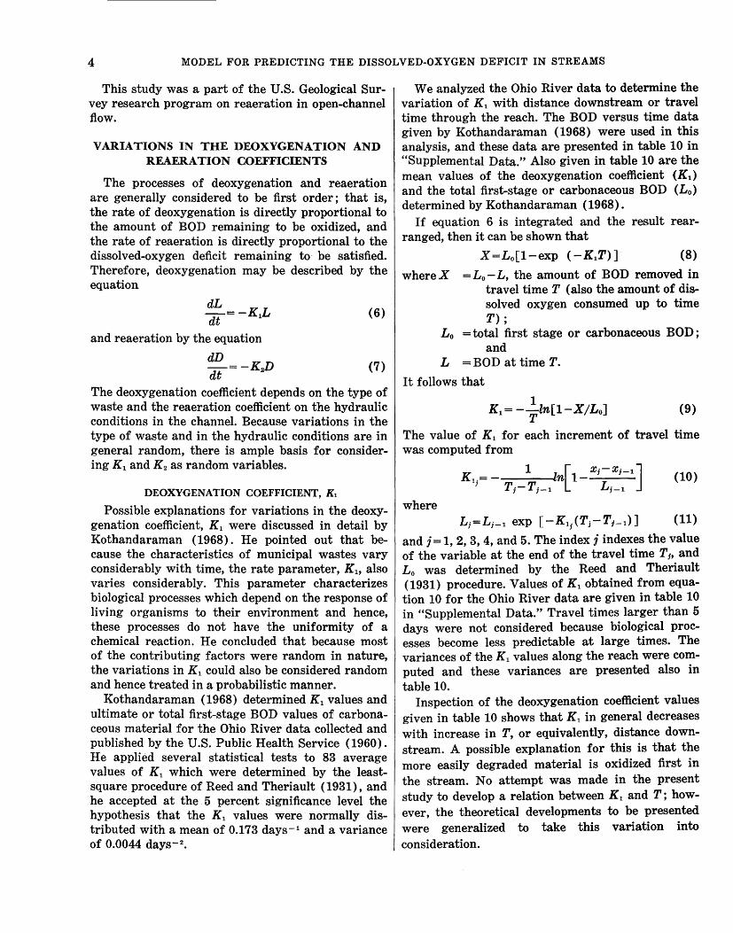
4 MODEL FOR PREDICTING THE DISSOLVED-OXYGEN DEFICIT IN STREAMS

This study was a part of the U.S. Geological Sur­vey research program on reaeration in open-channel flow.

VARIATIONS IN THE DEOXYGENATION AND REAERATION COEFFICffiNTS

The processes of deoxygenation and reaeration are generally considered to be first order ; that is, the rate of deoxygenation is directly proportional to the amount of BOD remaining to be oxidized, and the rate of reaeration is directly proportional to the dissolved-oxygen deficit remaining to- be satisfied. Therefore, deoxygenation may be described by the equation

dL dt = -K1L

and reaeration by the equation

dD -=-K2D dt

(6)

(7)

The deoxygenation coefficient depends on the type of waste and the reaeration coefficient on the hydraulic conditions in the channel. Because variations in the type of waste and in the hydraulic conditions are in general random, there is ample basis for consider­ing K1 and K2 as random variables.

DEOXYGENATION COEFFICIENT, K1

Possible explanations for variations in the deoxy­genation coefficient, K1 were discussed in detail by Kothandaraman ( 1968) . He pointed out that be­cause the characteristics of municipal wastes vary considerably with time, the rate parameter, K1, also varies considerably. This parameter characterizes biological processes which depend on the response of living organisms to their environment and hence, these processes do not have the uniformity of a chemical reaction. He concluded that because most of the contributing factors were random in nature, the variations in K1 could also be considered random and hence treated in a probabilistic manner.

Kothandaraman (1968) determined K1 values and ultimate or total first-stage BOD values of carbona­ceous material for the Ohio River data collected and published by the U.S. Public Health Service (1960). He applied several statistical tests to 83 average values of K1 which were determined by the least­square procedure of Reed and Theriault (1931), and he accepted at the . 5 percent significance level the hypothesis that the K1 values were normally dis­tributed with a mean of 0.173 days-1 and a variance of 0.0044 days- 2

•

We analyzed the Ohio River data to determine the variation of K1 with distance downstream or travel time through the reach. The BOD versus time data given by Kothandaraman (1968) were used in this analysis, and these data are presented in table 10 in "Supplemental Data." Also given in table 10 are the mean values of the deoxygenation coefficient (K1) and the total first-stage or carbonaceous BOD (Lo) determined by Kothandaraman ( 1968) .

If equation 6 is integrated and the result rear­ranged, then it can be shown that

X=Lo[1-exp ( -K1T)] (8)

where X = Lo- L, the amount of BOD removed in travel timeT (also the amount of dis­solved oxygen consumed up to time T);

L 0 =total first stage or carbonaceous BOD; and

L =BOD at timeT.

It follows that

1 K1= --ln[1-X/Lo]

T (9)

The value of K1 for each increment of travel time was computed from

1 zn[t X;-X;-1] T1- T;-1 L;-1

(10)

where L;=L;-1 exp [-K1,{Tj-T1-1)] (11)

and j = 1, 2, 3, 4, and 5. The index i indexes the value of the variable at the end of the travel time T, and Lo was determined by the Reed and Theriault (1931) procedure. Values of K1 obtained from equa-tion 10 for the Ohio River data are given in table 10 in "Supplemental Data." Travel times larger than 5 days were not considered because biological proc­esses become less predictable at large times. The variances of the K1 values along the reach were com­puted and these variances are presented also in table 10.

Inspection of the deoxygenation coefficient values given in table 10 shows that K1 in general decreases with increase in T, or equivalently, distance down­stream. A possible explanation for this is that the more easily degraded material is oxidized first in the stream. No attempt was made in the present study to develop a relation between K1 and T; how­ever, the theoretical developments to be presented were generalized to take this variation into consideration.

VARIATIONS IN THE DEOXYGENATION AND REAERATION COEFFICIENTS 5

It was also observed that the variance of the initial values of K1 at T = 0 was considerably larger than the variance of K 1 along the reach for a spe­cific initial value of K11• A Chi-square test of the initial values of K1 showed that, at the 5 percent significance level, the data were compatible with the assumption that they were normally distributed with a mean of 0.205 days-t, and a variance of 0.00538 days- 2

• Two extreme values of K1, com­puted from observations numbered 37 and 80, were neglected in the analysis. The coefficient of varia­tion of the initial K1 values was 0.357. The average variance of the K1 values along the reach was 0.0015 days- 2

• It was assumed that the K 1 values along the reach were normally distributed with the above mentioned variance, but this hypothesis could not be tested, because for T < 5 days, each series of ob­servations contained only four data points.

The coefficient of variation, Cv, of the mean values of the deoxygenation coeffiicent, KH for the Ohio River data was 0.066/0.173 or 0.38. In the present study, no attempt was made to substantiate the pres­ence of the same K1 value in all streams; however, as a first approximation, the coefficient of variation of K1 is assumed to be

(12)

Thus, the assumption is that the dispersion or spread of the K1 values about the mean is essentially the same as in the Ohio River data. Although the data in table 10 indicate that there is a difference be­tween the variance of the initial values of K1 and the variance of the K1 values along the river reach, a coefficient of variation of 0.35 will in general be used to estimate both of these variances. The differences obtained in the probability distribution of the dis­solved-oxygen deficit by considering different values of Cv(Kl) for the initial values of K1 and for the values of K1 along the reach, and by assuming the same Cv (Kl) for both variances, are discussed in the examples presented later.

The probabilistic model to be described in the next section is capable of considering both variations in the initial value of K1 and variations in K1 along the river reach. Another possibility is that the initial K1 values are deterministic, but the variance of K1 is very large during the first few hours. No data were available to test this supposition.

REAERATION COEFFICIENT, K2

In general, the reaeration coefficient, K2, of a stream may be considered as a property of the flow in the channel. As such, the variation with time of

K 2 may be defined as the sum of a constant term, a periodic component, and a random component (Ma­talas, 1971). The constant term may under some cir­cumstances itself be a function of time or distance downstream. The periodic component results from seasonal changes or perhaps diurnal changes, for example, in the quantity of flow. The random com­ponent has no simple physical explanation but is the resultant of a very large number of physical causes; for practical purposes, this random component may be considered as the inherent characteristic of tur­bulent flow (Matalas, 1971). Because the intensity of turbulence at a point in a stream has an approxi­mately normal distribution (Batchelor, 1959), there is in turn a basis for considering K2 as a normally­distributed random variable.

The K 2 data of Churchill, Elmore, and Bucking­ham (1962) for streams of the Tennessee Valley are generally considered to be the best available data for natural streams. The reaeration coefficient was com­puted from

K _ 1 .z [ Cs-Ci J 2-- n J T1- T1-1 Cs- C1-1

(13)

where C8 =saturation concentration of dis-solved oxygen;

C =dissolved-oxygen concentration; j, j -1 =value of variable at the end of the

time of travel T;, T1-1; and c.'l-CO =dissolved-oxygen deficit, where Co is

the dissolved-oxygen concentra­tion at the upstream end of the reach, assumed to be known.

Several equations were developed by multiple re­gression analysis, and each of these equations was tested by comparing computed K2 values with the geometric means of the experimental K2 values for each reach studied. The equation recommended for use by Churchill, Elmore, and Buckingham ( 1962) was

K22o = 5.026Vo.969H-t.a7s (14)

where V =mean velocity of flow in feet per second;

H =mean depth of flow in feet; and K2

20 =reaeration coefficient in days-1 at

20°C.

For V in metres per second and H in metres, the constant term in equation 14 is 2.178. Equation 14 had a correlation coefficient of 0.822.

Kothandaraman (1968) conducted a regression analysis of the Churchill, Elmore, and Buckingham

6 MODEL FOR PREDICTING THE DISSOLVED-OXYGEN DEFICIT IN STREAMS

(1962) data using arithmetic mean values for each reach and obtained

Kz2o = 5.827Vo.924H-t.7o5 (15)

with a correlation coefficient of 0.917 (for V in metres per second and H in metres, the constant 1

term in equation 15 is 2.304) . He then analyzed the ', distribution of the percentage errors, with the per­centage error defined as (Kz-K2p) (100)/K2p where Kz is the arithmetic mean value, and Kzp is the value predicted by equation 15. He found that the per­centage errors were approximately normally dis­tributed with a mean of zero and a standard devia­tion of 0.368. His analysis assumes that the value of Kz20 given by equation 15 is correct and that devia­tions from it are probabilistic in nature; it also as­sumes that once a process starts with a certain value of Kz, the rate of reaeration is constant for the reach.

In the present study, we assumed that the devia­tions of measured values of Kz for a specific reach of stream from the mean of all the measured K 2 values for that reach were normally distributed. This as­sumption is in contrast with that of Kothandaraman ( 1968) in that he assumed that deviations of the means of the experimental Kz values from Kz values computed from equation 15 were normally dis­tributed. The arithmetic means, variances, and the coefficients of variation estimated from the K 2 data of Churchill, Elmore, and Buckingham (1962) are presented in table 11 in "Supplemental Data." The mean value of the coefficients of variation for all streams studied was 0.307. Therefore, for our study, we have assumed that the coefficient of variation of the reaeration coefficient is 0.3, or

(16)

CORRELATION BETWEEN DEOXYGENATION AND REAERATION COEFFICIENTS

(1969) who used the stochastic model of Thayer and Krutchkoff ( 1966) to estimate the correlation coeffi­cient. The correlation coefficient was defined as

Correlation coefficient covariance

(17) [(BOD variance) (D variance) )112

The correlation study was run with an initial BOD input (L0 ) of 12.4 mg/1 (milligrams per litre), a saturation concentration (C8 ) of 10.4 mg/1, an ini­tial dissolved-oxygen concentration (Co) of 5 mg/1, and a value of 0.1 mg/1 for the ~-parameter of Thayer and Krutchkoff ( 1966). Different values of K 11 K2, and T were used, and the resultant correla­tion coefficients between BOD and dissolved-oxygen concentration obtained by Moushegian and Krutch­koff (1969) are presented in table 12 in "Supple­mental Data." The correlation coefficient is positive at all times which implies that the correlation coeffi­cient between BOD and Dis negative.

Moushegian and Krutchkoff ( 1969) found that in­terpretation of the results of the correlation coeffi­cient study was difficult, but in general it was ob­served that the correlation coefficient between BOD and dissolved-oxygen concentration decreased as time of travel increased and the difference between K2 and K1 increased. On the other hand, as the time of travel becomes small, correlation between BOD and D approaches - 1. This may be seen as follows : for an initial dissolved-oxygen deficit of zero and small travel times, the exponentials in equations 3 and 4 may be approximated by their Taylor series expansions. Hence

(18)

and (19)

where ~T=an incremental value of the time of travel.

The Moushegian and Krutchkoff ( 1969) study yielded no information on the possible correlation between K1 and Kz. Therefore, in the present study, the correlation coefficient between Kl- and K2 was assumed to have the value

(20)

Increased turbulence and mixing in a stream re­sult in a more rapid rate of reaeration and hence a larger K2 and also a larger K1 as a result of in­creased bacterial degradation of wastes; conversely, lower levels of turbulence result in smaller K1 and Kz values. Similarly, an increase in temperature in­creases both K1 and K2. Therefore, a positive corre­lation between K1 and K2 is expected.

1 This correlation coefficient was applied to the K1 and K2 values at the same instant of time, although the presence of a small lag period is possible. The effect of different correlation coefficient values on the

Although the interdependence between BOD and dissolved-oxygen deficit, D, is known, little effort has been directed toward determining the numerical value of the correlation coefficient for BOD and D. There has, however, been one theoretical approach j'

to the problem by Moushegian and Krutchkoff oxygen-deficit distribution will be discussed in the examples to be presented.

DEVELOPMENT OF THE PROBABILISTIC MODEL 7

DEVELOPMENT OF THE PROBABILISTIC MODEL

SOLUTION OF EQUATIONS FOR LONGITUDINAL PROFILES OF BOD AND DISSOLVED­

OXYGEN CONCENTRATION

The longitudinal profiles of the BOD and dis­solved-oxygen concentration downstream from a source of organic biodegradable waste are described by equations 1 and 2, respectively. The assumptions inherent in these equations were discussed previous­ly. With the additional assumptions of (1) the ef­fect of longitudinal dispersion on the BOD and dis­solved-oxygen concentration profiles is negligible relative to other factors; and (2) the effect of photo­synthesis and respiration is negligible; equations 1 and 2 reduce, respectively, to

oL oL -+ V-=- (Kl +K3)L+La (21) at ox and

ac ac -+ V-=K2C8 -K1L+Ca-DB-K2C. (22) at ax These equations, as well as equations 1 and 2, as­sume that the water temperature, and hence the saturation concentration of dissolved oxygen, is constant.

The effect of longitudinal dispersion on the BOD and dissolved-oxygen concentration profiles for steady-state and uniform flow conditions was dis­cussed by Dobbins (1964) who concluded that the effect was negligible for the largest value of Dx known at that time. A much larger value was found later by Yotsukura, Fischer, and Sayre (1970), but the mean flow velocity was also large; and according to Dobbins' analysis, the effect of dispersion would still be negligible. In estuaries where dispersion be­comes large and velocities small, the effect of longi­tudinal dispersion cannot be neglected. The effect of photosynthesis may be extremely important in cer­tain situations; the literature and procedures for treating photosynthesis were discussed by Bennett and Rathbun (1972). The water temperature may increase in the downstream direction as a result of both natural and manmade causes ; this problem was considered by Liebman and Lynn ( 1966) . Thus, longitudinal dispersion, photosynthesis, and changes in water temperature may be important in certain situations; for the present study, however, they were neglected.

Following Li (1962), equations 21 and 22 were solved for a stream system with the following characteristics :

1. Hydraulic conditions may vary with distance downstream but are steady at each cross section.

2. The BOD and dissolved-oxygen concentration at the cross section at which the waste is added to the stream may be functions of time; in­herent in the assumption of one-dimensionali­ty is the requirement that the distance neces­sary for complete lateral and vertical mixing of the BOD be small relative to the distance downstream to the cross section ( s) of interest.

3. The rate coefficients K1, K2, and K3 are functions of the time of travel or distance downstream.

4. The distributed source and sink terms, that is, Ca, La, and DB, vary with distance downstream but are steady at each cross section.

Time of travel, T, and distance downstream, x, may be interchanged through the relation

T=rx ~ lo V (23)

Details of the solution have been presented previous­ly (Esen, 1971), and only the results will be pre­sented here.

For the longitudinal profile of the BOD, the equa­tion obtained was

- (Kt+K3)dT o [ T [ + [<Kl+K3)dT' ]

L=e f(~)+1TLae dT (24)

where~ is given by r:c dx

~=t-Jo v; (25)

/(~) =function describing the variation with time ~of the BOD at the upstream end of the reach; and

T, T' =dummy variables of integration.

Comparison of equation 24 with equation 3, which !fescribes the BOD profile for the approach of Streeter and Phelps ( 1925), shows the differences in the results. If the BOD at the upstream end of the reach is independent of time, K3 and La are zero, and K1 is independent of time of travel in the reach, then equation 24 reduces to equation 3.

8 MODEL FOR PREDICTING THE DISSOLVED-OXYGEN DEFICIT IN STREAMS

For the longitudinal profile of the dissolved-oxy­gen deficit, the equation obtained was

where

iT (Kt+Ka)dT'

I= [T Lae dT; and (27)

F (') =function describing the variation with time' of the dissolved-oxygen concentration at the upstream end of the reach.

In equation 26, the term C8 -F(') is the dissolved­oxygen deficit at the upstream end of the reach; the first integral term is the net effect of the addition of dissolved oxygen along the reach by all processes other than reaeration and photosynthesis and the removal of dissolved oxygen by the benthal layer on the stream bottom ; the second integral term is the BOD added at the upstream end of the reach; and the third integral term is the BOD added along the reach.

Comparison of equation 26 with equation 4, which describes the longitudinal profile of the dissolved­oxygen deficit for the approach of Streeter and Phelps (1925), shows the differences in the results. If the dissolved-oxygen concentration at the up­stream end of the reach is independent of time, La, DB, Ca, and K3 are zero, and K1 and K2 are inde­pendent of time of travel in the reach, then equation 26 reduces to equation 4.

Equations 24 and 26 describe the longitudinal pro­files of the BOD and dissolved-oxygen deficit, respec­tively, for a stream system in which the rate coeffi­cients KlJ K2, and K3 are unknown functions of the time of travel. Application of these equations to the estimation of the probability distributions of the BOD and the dissolved-oxygen deficit for a stream system in which K1 and K2 are normally distributed random variables is described in the following sections.

RANDOM WALK MODELS

There is considerable justification, as discussed previously, for considering the deoxygenation coeffi­cient, KlJ and the reaeration coefficient, K2, as ran-

dom variables. Therefore, it is possible to consider

that the values of the integrals iT K1dT and [T K 2dT

are attained as a result of a simple random walk.

DEOXYGENATION COEFFICIENT, K1

Assume that in a time interval of A.T the quantity K1A.T can take only two possible values, K1 (T) A.T +A.K1 and K1(T)A.T-A.K1. To these two values the following probabilities are assigned:

P[l(1 (T) A.T=K] (T) A.T+ A.K1] =p1 (A.K1) (28)

P[K1 (T) A.T =K1 (T) A.T- A.K1] = ql (A.Kl) (29)

where K1 (T) =mean value of K1 at time of travel T and P1 (A.Kl) + ql (A.Kl) = 1. For the present analysis, it will be considered that A.K1 is constant.

Let us further assume that

lim [q1(A.K1)-pl(A.K1)] a1 T

(30) A.K1

lim (A.Kl) 2 f3 T aT~ 1 aK1~0 A.T

(31)

where a1 and {31 are finite. Then the probability dis­tribution of K1 is found to be normal (Bailey, 1964; Feller, 1968) with a mean of K1 -al/31 and a vari­ance of {31. For the limiting variance to remain finite, (A.K1)2 1 A.T must be of the order of unity, and for the mean to remain finite, p 1- ql must be of the order of A.K1. The equations of this section satisfy these conditions.

These concepts were applied to equation 24 to esti­mate the probability distribution of the BOD for a stream system in which K1 is a random variable. In this analysis, the following assumptions were made:

1. The BOD added along the reach is much smaller than the BOD added at the upstream end of the reach, that is

1T LadT<«f(');

-1"(Kt+Ks)dT

and hence the variance of the term I e is negligible, where I is defined by equation 27; and

2. The rate constant for the removal of BOD by sedimentation and adsorption, K3, is deter­ministic throughout the river reach under con­sideration, that is, independent of flow time.

These assumptions are valid for many situations observed in natural streams; in fact, the effects of La and K 3 were completely neglected by several in-

DEVELOPMENT OF THE PROBABILISTIC MODEL 9

vestigators (Streeter and Phelps, 1925 ; Kothan­daraman, 1968). Considering K 3 as a random vari­able does not introduce any complications into the analysis if K3 is considered as normally distributed with known mean and variance. For appreciably large values of La, the probability distribution of the BOD cannot be found analytically, but Monte Carlo methods can be efficiently used.

Details of the development of the probability dis­tribution of the BOD have been presented previously (Esen, 1971). It was found that the BOD was dis­tributed according to the lognormal distribution, or

for

and

fL( ·) =0 for LL.J exp (- [T (K1 +K3)dT) (32)

The mean value of L for any time of travel Twas found by integrating the product of L and the den­sity function between the limits - oo and + oo. The result was

L=exp[ In fW- f (K,+K,)d.+Ta,p,+ T~, J +] exp (-iT (K1 +K3)dT) (33)

Similarly the variance of L at any time of travel T was found by integrating the product of (L- L) 2 and the density function between the limits - oo and + oo, and the result was

var (L) =exp[ 2[ln f(t)-r (K, +K,)d.+Ta,p,]

+2T'p,] -exp[ 2[ln fW-r (K,+K,)d.

+ Ta,p,] + T•p, J (34)

The probability density function of L given by equation 32 reduces to that of Kothandaraman (1970), if K3 and La are 0 and K1 is considered to be independent of the time of travel. However, one of the advantages of the random walk model from which equation 32 was developed is that it can con-

sider K1 as well as the mean and variance of K1 as a function of time of travel. Thus in the most general case, /31 and a1 are functions of the time of travel. If the variance of K1 is considered as constant through­out the river reach of interest, /31 is constant, and if it is further considered that the mean value of K1 is also constant, then a1 can be taken as zero. The mean and variance of K1 are measurable quantities, and numerical values can be assigned to K11 a1, and /31.

REAERATION COEFFICIENT, K 2

Proceeding exactly analogously as for the deoxy­genation coefficient, we assume that in a time inter­val of AT the quantity K2AT can take only two possi­ble values, K2(T)AT+AK2 and K2(T)AT-AK2. To these two values, the following probabilities are assigned:

P[K2 (T)AT=K2 (T)AT+AK2] =p2(AK2) (35)

P[K2(T)AT=K2(T)AT-.AK!] =q2(AK2) (36)

where K2(T) is the mean value of K2 at time of travel T and P2 (AK2) + q2 (6K2}~ 1. Let us further assume that

lim l1KNO

[ q2 (AK2) -p2 (AK2)]

AK2

1~~ (:~2 )2

f32T l1KNO

T (37)

(38)

where a2 and /32 are finite. Then the probability dis­tribution of K 2 is found to be normal (Bailey, 1964; Feller, 1968) with a mean of K2-a2/J2 and a vari­ance of fJ2· These equations also satisfy the condi­tions previously given for the limiting variance and the mean to remain finite.

Because of mathematical complexities, it was not possible to apply this random walk model for the re­aeration coefficient to equation 26 and obtain ana­lytically the distribution function of the dissolved­oxygen deficit. Therefore, the distribution of the oxygen deficit was estimated by using a Monte Carlo simulation technique.

MONTE CARLO SIMULATION TECHNIQUE FOR DISSOLVED-OXYGEN DEFICIT

The Monte Carlo simulation technique is a method by which a complex system with random components is numerically operated by random numbers chosen in such a manner that they simulate the physical behavior of these components. In the general sense, each random component of the system is represented by a numerical value randomly chosen from some probability distribution.

10 MODEL FOR PREDICTING THE DISSOLVED-OXYGEN DEFICIT IN STREAMS

Monte Carlo simulation essentially involves three steps:

1. Select representative probability distributions which will simulate the physical behavior of the random components of the system.

2. Generate numerical values of the random vari­ables from the probability distributions.

3. Use variance-reducing techniques to accelerate the computations.

A random walk model is well suited to simulation by Monte Carlo methods because each random com­ponent (the increments added to K1 or K 2 in the present study) is allowed to take only two possible discrete values. This requires the simplest of random variable generation techniques, the generation of uniformly distributed random variables. The meth­ods for the generation of uniformly distributed ran­dom variables are discussed in various books (such as Hammersley and Handscomb, 1964) , and almost all digital computers have a built-in subroutine avail­able for this purpose.

The determination of the probability distribution of the dissolved-oxygen deficit is based on equation 26 which may be written

where

-12' K2flr [ lT K2flr'

B=e 0

~s-F(t) +iT (DB-Ca)e dr

T lT (K2-K1-Ka)d,_' J + i K 11 e dr (40)

Additional assumptions are necessary besides those made in the development of the model for the proba­bility distribution of the BOD. These are: 1. the initial dissolved-oxygen deficit, C8 -F(t), is

small and the variance of the term [C8 -F(t)]

-12'K2flr

e is small ; and 2. the difference between the benthal demand term,

DB, and the term for the addition of dissolved oxygen along the reach, Ca, is small, and the

-12'K2flr

variance of the term e

[

1TK2flT' J iT (DB-Ca) e o d1' is small.

With these assumptions and approximating the integrals in equation 39 by finite sums, it follows that

Cs-C-B= /(t) exp (- 2: K2iAT) K -K 11_K

n [ -.K

i= 1 2t lt 3

+ n'i:l K,,(K,<+ 1 -K,)- (K,,-K,)K,<+, .

1 (K2.-K1.-K3) (K2.+1-Kt.+1-K3)

1,= t t t t

exp { .± (K,;-K,;-K,) !>.T} J=1

+ K _i1

n -K exp { 1: (K2i-Kli-K3)AT}] ~ ~ 3 • 1 J=

(41)

Note that for nAT=T, K11=K12 = ... =K1n' K3=0,

and K21 =K22 = ... =K2n' equation 41 reduces to the classical oxygen sag equation of Streeter and Phelps (1925) (recall eq 4).

If K a should be a normally distributed random variable like K1 and K2, then Monte Carlo simulation requires three sets of uniformly distributed randoll} numbers to be generated (one each for K11,

K2i' and Kai). There is no evidence at present, how­ever, to suggest that Ka is a random variable. Hence, Ka was considered to be deterministic in the present study.

The determination of the probability distribution of the oxygen deficit at any time of travel, T, by Monte Carlo simulation involves the following steps:

1. Experimentally determine the mean and vari-ance of K1 and K2 and the correlation coeffi­cient between K1 and K2; or by experimentally determining the means, estimate the variance of K1 and K2 from equations 12 and 16, respec­tively, and the correlation coefficient between K1 and K2 from equation 20.

2. Choose an integer n and determine AT from AT=T/n.

3. Determine AK1 and AK2 from equations 31 and 38, respectively, as

AK1 = y /3tT AT

AK2 = y f32T AT

where /31 =variance of K1; and

/32 =variance of K2.

4. If the mean values of K1 and K2 are assumed to be time-independent, then a1 = a2 = 0 and Pt = P2 = 0.5. For time-dependent mean values of K1

DEVELOPMENT OF THE PROBABILISTIC MODEL 11

and K2, determine a1 and a2 from mean (Kl) =K1-.atf31 and mean (K2) =K2 -a2(32 (Kl and K2 will be estimated as the values of K1 and K2 at T = 0), and compute P1 and P2 from equa­tions 30 and 37 as

Pt = (1-atAKt/T) /2

P2= (1-a2aK2/T)/2.

5. Compute B from equation 40 with known values of Cs, F ('),DB, Ca, La, K 3 , and mean values of K1 and K2, and consider B as deterministic at any time of travel, T. If B is not deterministic, see below for the procedure to use.

6. Generate two sets of n uniformly distributed random numbers, R11 and R2

1, between 0 and

1, and compute K11aT and K2iaT as

K11aT=K1aT+aK1 R1i<P1 KtiAT=KtAT-AKt Rti"?::pl K21AT=K2AT+AK2 Rt;<Ph R2i~[1-r(KH K2)]/2

or R11~p1, R2i< [1-r(KH K2) ]/2

K21AT=K2AT-AK2 Rt;<PH R2i< [1-r(Kt, K2) ]/2 or

R11~1, R2i::::::,.[1-r(KH K2) ]/2

7. With the value of B determined in step ( 5) and K11AT and K2JAT values determined in step (6), compute the oxygen deficit or (C8 -C) from equation 41.

8. Repeat steps 6 and 7 m times to obtain an esti­mate of the probability distribution of the oxy­gen deficit.

The assumptions made in the development of equations 32 and 41 are reasonable for many streams. However, if the values of La, Ca, Cs-F(,), and DB- C a are large and K 3 is normally distributed rather than deterministic, Monte Carlo methods can still be used efficiently. However, writing the inte­grals involving I as finite sums requires very com­plicated expressions, and it is more convenient to use a series of difference equations which can be solved easily on a digital computer. The difference equa­tions for the equations describing the BOD and oxygen deficit distributions (eqs 24 and 26, respec:. tively) are

- (K11+Ka1 ).iT L (j) L (j) = e [ L (i -1) + K a K

lj+ 3;

(K11+Ka1).iT

(e -1)]

j = 1' 2, . . . ( 42)

L(O) =!(') (43)

K1. (K21 -K11-Ks1)-iT

+L(j-1) K2.-K:.-K3. (e -1) J J J

K11La (j) K21-iT

+ (e -1) K2j (K11 + K3)

K11La(j) (K21-K11-Ka1)-iT J -----------------------(e -1) (K11 +Ka1) (K21-Kt1-Kai)

j=1, 2, ... C(O) =F(')

(44) (45)

where T = j aT for a specific value of the argument i. Therefore, if the variance of B cannot be ne­

glected, equations 42, 43, 44, and 45 are used recur­rently in step (7) of the procedure rather than equa­tion 41. If the variance of the initial K1 values is different from the variance of the K1 values along the river reach, then the initial K1 values can be se­lected from a normal distribution with known mean and variance. The total variance of K1 equals the sum of the variance of the initial values of K1 and the variance of the K1 values along the reach.

The sampling method used in this study is refer­red to as "Straightforward Sampling." This method is based on the premise that the uncertainty in the mean value obtained by a Monte Carlo technique is always reduced when the sample size is increased. A number of methods are available for reducing the variance of the results obtained with the same m value used in the straightforward sampling (Kahn, 1957; Hammersley and Handscomb, 1964). How­ever, because of the complexity of the equations used in the determination of the probability distributions of the oxygen deficit, these methods could not be used in the present study. A flow chart of the straight­forward Monte Carlo simulation procedure used in the present study is presented in figures 22, 23, and 24 in "Supplemental Data."

APPLICATION OF THE TECHNIQUE AND DISCUSSION OF RESULTS

To demonstrate the application and versatility of the stochastic model, a hypothetical example consist­ing of three parts was used. In addition, the model was applied to data from the Sacramento River. De­tails of these examples are presented in the follow­ing paragraphs.

HYPOTHETICAL EXAMPLE

The basic data used in the hypothetical example consisted of

12 MODEL FOR PREDICTING THE DISSOLVED-OXYGEN DEFICIT IN STREAMS

K1 =0.15 days-1;

K,2=0.50 days- 1 ;

f (') = 10 mg/1 ; and

C.s-F(') =0 mg/L

In addition, the effects of D{J), K3 , La, and Ca on the profiles of the BOD and oxygen deficit were assumed to be negligible. The quantities f(O and C8 -F(') are, respectively, the BOD and oxygen deficit at the upstream end of the reach.

The probability distribution of the oxygen deficit was estimated using three sets of conditions. In the first case, the variances of the initial values of K1 and of the values of K1 along the reach were assumed to be equal, K1 and K2 were assumed to be uncorre­lated, and the variance of K 2 was assumed to be con­stant. In the second case, the variances of the initial values of K1 and of the values of K1 along the reach were different, K1 and K2 were assumed to be uncor­related, and the variance of K2 was assumed to be constant. The third case assumed that the variances of both K1 and K2 were constant and also a constant correlation coefficient between K1 and K2 was as­sumed. In all three cases, the mean values of K1 and K2 were assumed to be independent of time of travel, and therefore a1 =a2=0.

Details of the three cases are as follows :

Case 1: The coefficients of variation, Cv (K1) and Cv (K2), were assumed to be 0.35 and 0.3, respective­ly, as discussed previously (recall eqs. 12 and 16). From these values, the variances of K1 and K2 were computed as

var (K1) =,81 = [Cv(Kl)K1] 2

= [ (0.35) (0.15) ] 2=0.00276 days-2

var (K2) =,82= [Cv(K2)K2] 2

= [ (0.3) (0.50) ] 2=0.0225 days-2

Case 2: The analysis of the Ohio River data dis­cussed previously showed that the variance of the K1 values along the reach was 0.0015 days-2 for an initial mean K1 value of 0.205 days-1. Hence, the variance of the K1 values along the reach for the hypothetical example was estimated as

,8';= [ (y0.0015/0.205)0.15)2=0.00080 days-2

The variance of the initial values, K11

, therefore is

,8'1 = ,81- ,8':

= 0.00276-0.00080 = 0.00196 days-2

The initial values, K11

were selected randomly from a normal distribution with a mean of 0.15 and a variance of 0.00196. Twelve uniformly distributed

random numbers, R1i' were generated and K11 was computed from

12 K11 = y/0.00196 [ L R1i- 6] + 0.15

~=1

Then the Monte Carlo techniques were applied with

,8"=0.00080 days-2 and ,82=0.0225 days-2. 1

Case 3 : The third case was essentially the same as the first case except that K1 and K2 were assumed to be linearly correlated with a correlation coefficient of 0.5.

Equation 41 with B=O was used in all three cases for the estimation of the distribution of the oxygen deficit. The mean values of K1 and K2 were assumed to be independent of time, hence a1 = a2 = 0. It follows that P1 =p2=0.5.

The mean, variance, and the 10 percentile and 20 percentile limits of the oxygen deficit obtained for the three cases along with the oxygen-deficit values computed from the Streeter and Phelps ( 1925) equation (recall eq 4) using mean values of K1 and K2 are presented in table 1. The 10 percentile and 20 percentile limits of the oxygen-deficit distribution indicate the oxygen-deficit values for which 10 per­cent and 20 percent, respectively, of the deficit values are larger. The frequency distributions of the oxygen deficits are plotted in figures 1, 2, and 3. The mean values of the oxygen deficits and the 10 per­centile and 20 percentile limits are plotted in figure 4 as a function of time of travel.

TABLE 1.-Dissolved-oxygen deficit from equation 4 and sig-nificant parameters of the stochastic, oxygen-deficit distri-bution

Vari-ance 10 per- 20 per-

Time, Deficit Mean of centile centile T (eq 4) deficit deficit limit limit

(days) (mg/l) (mg/11 (mg/1)~ (mg/1) (mg/1)

Case 1

1 1.09 1.04 0.121 1.48 1.31 2 1.60 1.56 .315 2.29 2.04 3 1.78 1.73 .528 2.64 2.33 4 1.77 1.80 .575 2.84 2.34 5 1.67 1.82 .931 3.07 2.45

Case 2

1 1.09 1.07 0.129 1.54 1.36 2 1.60 1.67 .347 2.46 2.19 3 1.78 1.72 .400 2.51 2.23 4 1.77 1.81 .668 2.91 2.43 5 1.67 1.64 .580 2.62 2.20

Case 3

1 1.09 1.03 0.101 1.41 1.29 2 1.60 1.49 .191 2.06 1.86 3 1.78 1.67 .266 2.36 2.09 4 1.77 1.83 .372 2.68 2.28 5 ------- 1.67 1.61 .367 2.44 2.09

DEVELOPMENT OF THE PROBABILISTIC MODEL 13

T=2 Days T=3 Days

,-

,--_ n ,___

->- -u -z UJ :::> 0 UJ a:: LL.

c j d 0 2 13 o. 4·

UJ > i= c( ...J UJ 0.8 a:: I - I I I I I I I I

0.6 - T=4 Days T=5 Days -----

0.4 - - r---- - >---- r-- --

r----0.2 -

~I rl -

------- I I 0 0 1 2 3 4 5 3 4 0 2

OXYGEN DEFICIT, IN MILLIGRAMS PER LITRE

FIGURE !.-Distribution of the oxygen deficit estimated for the conditions of ca'ie 1.

I--T-1 Day T=2 Days T=3 Days

r-

.--

1.0 r--

0.8 - -

0.6 -r--

-

- -

T-I r1

0.8 T=4 Days T=5 Days

0.6

0.4

L_! ___ __L__L___i__L___L_ _ __L__L-.I__L ___ _t___----------'---.J.....__._.----L.----'---'-_.___.___.__----L._--'-----'---------'--------'

3 0 2 3

OXYGEN DEFICIT, IN MILLIGRAMS PER LITRE

FIGURE 2.-Distribution of the oxygen deficit estimated for the conditions of case 2.

14 MODEL FOR PREDICTING THE DISSOLVED-OXYGEN DEFICIT IN STREAMS

1.4

1.2 - T=l Day

1.0

0.8

0.8 -------,r-----~

~~ll 0.2 1- 1 l

0.6-

0.4--

T=4 Days

T=2 Days

I

3 I

0

T=3 Days

11 I I I

LJI J j_jl_ 1 3

----~ ----·--r-·------, T=5 Days

0 L~~ ---::----___L___l __ L ___ ________L_____j_-~ ~I ~--l L ____________ ] __ ~ - ]~ j '==I - 3 4 0 1 2 3 4 0

OXYGEN DEFICIT, IN MILLIGRAMS PER LITRE

FIGURE 3.-Distribution of the oxygen deficit estimated for the conditions of _<;a.se 3.

The values of the variance of the oxygen deficit given in table 1 show that all three cases give com­parable results for small times of travel. However, as time increases, the variances of the deficit dis­tributions estimated for cases 1 and 2 become larger than the variance estimated for case 3. Case 3 is preferred in the present study because of the ex­pected positive correlation between K1 and K2. Re­call that r(Kh K2), the correlation coefficient be­tween K1 and K2, was assumed to be +0.5 for case 3. At the present time, there is no experimental data to assist in the assigning of an exact value or func­tion to the correlation coefficient. Inspection of the results presented in table 1 shows that the effect of the correlation coefficient on the oxygen-deficit dis­tribution increases as travel time T increases; how­ever, a time dependent r(Kh K2) whose average value is + 0.5 probably would not appreciably change the deficit distribution at large T.

To determine if r(K1, K2) could be estimated from r(BOD, D), the correlation coefficient between BOD and the oxygen deficit, a correlation study between BOD and the deficit for case 1 [r(Kh K2) =0] and

case 3 [r(K 1 , K2) =0.5] was made. The results are presented in table 2 and show that r(BOD, D) is rather insensitive to r(Ku K2). Hence, r(Kh K2) cannot be efficiently estimated from a knowledge of r(BOD, D) for the conditions considered in the pres­ent study.

The frequency distributions of the oxygen deficit presented in figures 1, 2, and 3 show that the deficit distributions become flatter and skewed to the right as time of travel increases. This type of skewness is especially favorable in the determination of proba­bilistic stream standards because the percentile lim­its of the oxygen deficit will be less sensitive to errors in the values estimated for the coefficients of variation of K1 and K2 and the correlation coefficient

TABLE 2.--Correlation coefficients between BOD and ozygen deficit ·

Time, T (days)

1 -----------2 3

Correlation coefficient (BOD, D) Case 1

r(K1,K2) =0

-0.94 -.66 -.40

Case 3 r(K1, K2) =0.5

-0.96 -.64 -.26

DEVELOPMENT OF THE PROBABILISTIC MODEL 15

UJ 0::: t: ..J

0::: UJ a.. en ~ <( 0::: (!)

:::::i ..J

~

z r: C3 Li: UJ 0

z UJ (!)

>->< 0

2

3

4 0

0

2

3

4 0

4 0

Case 1

Case 2

Case 3

__ [

2 3 4 5

-

20 Percent--------!

3

TIME, IN DAYS

10 percent---:

FIGURE 4.-Mean oxygen deficit and 10 and 20 percentile limits as a function of time for the oxygen-deficit distribu­tions estimated for the conditions of cases 1, 2, and 3.

between K1 and K2. On the other hand, the most probable deficit values would not be very informa­tive because of the flatness of the deficit distribution. Kothandaraman ( 1968) concluded that the most probable oxygen-deficit values of the deficit distribu­tions were closer to the observed deficits than deficits predicted by deterministic equations at all times. At small times of travel, this conclusion is probably valid because of the high peaks in the frequency dis­tributions. However, the largest time of travel that Kothandaraman (1968) considered was 0.73 day and for larger times of travel, the deficit distribu­tions became flatter and the most probable deficit value cannot be estimated accurately.

The deterministic critical time of travel, that is, the travel time at which the deficit, computed from the Streeter and Phelps ( 1925) equation, is maxi­mum, was 3.44 days for the conditions of the hypo­thetical example. The oxygen-deficit values pre-

sented in table 1 and the deficit profiles plotted in figure 4 show that critical time of travel for case 1 was not reached for the 5-day period considered. For cases 2 and 3, the critical time of travel was at some point between 3 and 5 days. Additional data points would be necessary to determine the critical time more exactly. In general, however, as will be dis­cussed in later sections, the stochastic critical time of travel was larger than the deterministic time of travel.

SACRAMENTO RIVER DATA

The stochastic model developed in previous sec­tions was also applied to data from the Sacramento River, Calif. A detailed description of the reach of the river where the BOD and oxygen-deficit data were collected is given by Thayer and Krutchkoff ( 1966) and the dissolved-oxygen concentration data for T < 6 days are presented in table 13 in "Supple­mental Data." In addition to the dissolved-oxygen data, Thayer and Krutchkoff (1966) give the follow­ing parameters for the reach :

K1 =0.35 days-1

K2=0.75 days-1

La=0.20 mg/1 per day

DB=0.10 mg/1 per day

K3 = 0.20 days-1

/(C) =Lo=6.8 mg/l=constant

Ca=9 mg/1

Cs-F(C) =Do=0.3 mg/l=constant

The effects of longitudinal dispersion and of the ad­dition of dissolved oxygen along the reach were neglected~

On the basis of these data, the variance of B in equation 41 was considered negligible, and the value B at any time of travel T was determined from equation 40 as

B 1 a e-K2T-e-(Kl+Ka)T KL [ - - J (K2-K1 -K3) (K1 +Kg)

+[C8 -F(t)]e-K2T+ -==-+ ·[1-e-K2T] - [DB K1La J -K2 K2 (K1 + K3)

For the above values, equation 40 becomes

B = e-0·75T[0.300 + 0.636 (1- eo·20T) + 0.303 (e0.75T -1)]

Following essentially the procedure used in case 3 of the previous section, and using the values of C, (Kl) ,Cv (K2), and r (KHK2) given by equations 12, 16, and 20, respectively, and the value of B deter-

16 MODEL FOR PREDICTING THE DISSOLVED-OXYGEN DEFICIT IN STREAMS

mined above, equation 41 was solved 200 times where T I !:lT was taken as 100. The values of the deficit computed from equation 39 with mean values of K1 and K2 and the mean, variance, and 10 percentile and 20 percentile limits of the oxygen deficit computed from the stochastic model are presented in table 3. The observed concentration of dissolved oxygen, that is, C = C.s- D = 9- D, is plotted in figure 5 together with the dissolved-oxygen concentration profile pre­dicted by equation 39 and the mean, 10 percentile, and 20 percentile limits of the stochastic deficit dis­tribution. The frequency distributions of the oxygen deficit are presented in figure 6. The variances of the experimental data are presented in figure 7 as a function of the time of travel; also shown in figure 7 are the variances predicted by the stochastic model of Thayer and Krutchkoff ( 1966) and the stochastic model developed in the present study.

The dissolved-oxygen concentrations and the 10 and 20 percentile limit lines plotted in figure 5 can be used to check approximately the predicted deficit distribution. If the predicted distribution is correct,

9.0,--------------,--------------UJ

TABLE a.-Significant parameters of the oxygen-deficit dis-tribution for the Sacramento River data

Vari-ance 10 per- 20 per-

Time, Deficit Mean of centile centile T (eq 39) deficit deficit limit limit

(days) (mgfl) (mg/H (mg/))2 (mg/l) (mg/1)

1 1.48 1.40 0.107 1.78 1.68 2 1.54 1.46 .119 1.87 1.71 3 1.28 1.34 .159 1.84 1.63 4 1.00 1.02 .166 1.54 1.28 5 .76 .85 .127 1.25 1.08

then the 10 percentile and 20 percentile lines should have about 10 percent and 20 percent of the data points below them, respectively. The number of data points below each of these lines was counted for times between 0.2 and 5 days. It was found that 9.5 and 23.5 percent of the points lay below the lines, in good agreement with the expected percentages of 10 and 20 percent.

The frequency distributions for the oxygen deficit presented in figure 6 do not flatten and become skewed to the right as time of travel increases, as do the frequency distributions for the hypothetical ex-

0::: 1-:::i

Measured concentration

0::: UJ a. ~ 8.5 <t: 0::: (.!)

:::i ...J

~

~ 8.0- •

z 0 ~ <t: 0::: 1-z ~ 7.5 z 0 u z UJ (.!)

>-X 0 7.0 '• 0 UJ > ...J 0 en en 0

Stochastic model (this study, eq. 41) Deterministic model (eq. 39)

6·5o~-------~--------2L_ _______ ~3 ________ 4L_ ______ ~5

TIME, IN DAYS

FIGURE 5.-Experimental dissolved-oxygen concentrations, mean dissolved-oxygen concentrations predicred by the deter­ministic model (eq 39), and mean, 10, and 20 percentile limits of the dissolved-oxygen concentrations predicted by the stochastic model ( eq 41) ; Sacramento River data.

DEVELOPMENT OF THE PROBABILISTIC MODEL 17

>­(.) z

1.50

1.00

0.50

-

r--

~ 0 0 0 LLI a:: IJ..

LLI > i= 1.50 <( ...J LLI a::

1.00

0.50

1---

1---

-

~-

I

,---

I

,----~-------- r T=l Day

--

1---

I--

,-

llr I 2 3

I I I I I I I

T=4 Days ,-- T =5 Days -

,--

-

I-- -r-

-

-

!-l h, I I I I I 0 0 ---------- lr-

2 3 0 2 3

OXYGEN DEFICIT, IN MILLIGRAMS PER LITRE

FIGURE 6.-Distribution of the oxygen deficit as estimated from equation 41; Sacramento River data.

ample (recall figs. 1, 2, and 3). This difference is apparently a result of differences in the values of the coefficients and parameters used in the computations.

There is considerable scatter in the oxygen-deficit variances plotted in figure 7, and as a result, it is difficult to decide which of the two models best fits the data. A disadvantage of the Thayer and Krutch­koff ( 1966) model is that the parameter ~ must be determined from the measured variance at some time of travel. They used a time near zero; however, be­cause of the small variances and considerable scat­ter in the data at this time, it seems likely that ~ cannot be estimated very accurately. On the other hand, the stochastic model developed in the present study does not depend on a measurement of the deficit variance for predicting the deficit variance as a function of travel time.

Thayer and Krutchkoff ( 1966) concluded that the oxygen-deficit variance is a maximum at the travel time when the deficit is maximum. For the Sacra­mento River data (see fig. 5), the maximum deficit

occurred between 1 and 2 days. On the other hand, figure 7 suggests that the deficit variance is a maxi­mum for a time of about 3 days. The stochastic mod­el predicted a similar behavior in that the variance increased rapidly for 3 days, then increased little be­tween 3 and 4 days (see table 3) . The occurrence of the maximum deficit variance at a time larger than the critical time of travel did not appear to cause Tc to shift downstream relative to the deterministic critical time of travel. However, the 10 and 20 per­centile limits of dissolved-oxygen concentration be­come rather flat between the second and third days.

ESTIMATION OF THE ACCURACY OF THE MONTE CARLO PROCEDURE

The accuracy obtained from the Monte Carlo sim­ulation procedure depends on the values chosen for m and n. Recall that m is the number of times the computations are repeated and that n, the number of steps in the random walk process, appeared in several equations where integrals were approxi-

18 MODEL FOR PREDICTING THE DISSOLVED-OXYGEN DEFICIT IN STREAMS

"' GJ a:: 1-::J a:: 1.&.1 a.. CJ)

~ <( a:: (.!J

::::i ...J

~ z LLi (.)

z ~ a:: <(

>

0.18

0.16

0.14

0.12

0.10

0.08

0.06

0.04

0.02

0 0 1 3

TIME, IN DAYS

• Observed variance

4 5 6

FIGURE 7 .-Observed and predicted variance of the oxygen­deficit distributions as a function of time; Sacramento River data.

mated by finite sums. The accuracy obtained in these equations depends on the functional form of K1 and K2; if they are constants, then the accuracy will be 100 percent; if they are functions of time, then some error will result from the approximation of the inte­grals. Although the accuracy of the simulation pro­cedure increases as m and n are increased, the com­putation time and resultant computer costs also increase. The development of equations for estimat­ing the accuracy of the Monte Carlo method is de­scribed in the following paragraphs.

The comparison of the central moments of K1T with the central moments of the limiting normal dis­tribution was used as the criterion for estimating the accuracy of the Monte Carlo procedure. Moments of K1T rather than K1 were compared because deter­mining the value of K1T as the result of a random walk process is physically more meaningful.

The probability that the diffusing particle of a simple random walk will be at some location after n

steps is distributed according to the binomial dis­tribution (Bailey, 1964). Hence, it follows analo­gously that the probability density function of K1T is

n P[K1T= L: K1r6.T- (n-2j) ~K1J =( 1!' )<P1);(q1)n-;

. 1 J J= (46)

Previously it was established, in the limit as ~T~o, ~x1~o, that K1 was normally distributed with mean K1-ad31 and variance /11 for constant K1. Analo­gously, it can be shown that K1T is normally dis­tributed with mean K1T-a1f31T and variance f31T2

•

Equation 46 gives exact values for the m~an and variance of K 1T even for very large values of ~T because the mean and variance depend only on a1 and /31 computed from equations 30 and 31. The third central moment of the limiting normal distribution is zero and therefore the error in the third central moment of K1T could not be computed as a percent­age difference. As an alternative, the difference be­tween the fourth central moments of K1T obtained from the limiting normal distribution, /L4 (KtT, N), and from the probability density function defined by equation 46, P.t (K1T, AT), was used as an indicator of the effect of the value of non the accuracy of the Monte Carlo simulation procedure.

The fourth central moment of the normal distribu­tion is

hence

p.4 (K1T, N) = 3f3~T4

Similarly from equation 46,

/L4 (K1T, AT) = (2~K1) 4JL.l (Ji) ( 47)

where j has a binomial distribution with parameters nand P1· The fourth central moment of a binomial distribution is

IL4=np1q1[1 + 3 (n -2)p1q1]

hence JL-1 (K1T, aT)= (2AK1) 4 [3 (np1q1)2

+np q -6np2q2] (48)

1 1 1 1

For small ~T /T, it follows from equation 30 and 31 that

1 T 1

exp ( -a2f3 ~T /T). 4 1 1 (49)

4

DEVELOPMENT OF THE PROBABILISTIC MODEL 19

Substituting equation 49 into equation 48 and not­ing that n = T I aT we obtain

P.4 (K1 T, aT= 3{3~T4 exp (- 2a~{3laT IT) + f3.~T3aT [4exp (-a~{31aTIT)-6exp (-2a~{31aTIT)]. (50)

The error, E, in the fourth central moment of K 1 T is defined as

E _ JL4 (K1T, aT) - P.4 (K1T, N)

P.4 (K1T, N) . (51)

Then, using equations 47 and 50, 1

E=--{3{32T4 [exp ( -2a.2a aTIT-1] + a 2T3aT 3f32T4 1 1P 1 P 1 L

[ 4 exp ( -a.:/31 aT./T) -6 exp (- 2a~{31aT IT)]}

Expanding the exponentials and taking the first two terms gives

E

For the special case when a.1 = 0, the expression for E becomes exact, and

2 aT E=--- (52)

3 T Thus, if n = T I ~T = 100, the error in the fourth

central moment of K _ T is less than 1 percent. The same arguments are also valid for the fourth central moment of K2T.

The effect of the choice of the integer m on the accuracy of the Monte Carlo procedure was esti­mated on the basis of the weak law of large numbers (Mood and Graybill, 1963), or

P[l Zm-P.I<e]~l-8

In this expression, Zm is the sample mean of a ran­dom sample of size m from a probability density with a mean of p. and a variance of u2, m is any in­teger greater than u2le28, and e>O and 0<8<1.

Chebyshev's inequality states that P[g(Z) >s] <E[g (Z) ]Is for a random variable Z and non-nega­tive function g (·),where E[g (Z)] indicates the ex­pected value of g (Z). Now, if we let g (Z) = (Zm- p.) 2 and s = e2, then

P[IZm- p.l 2<e2] ~1-E[ (Zm- p.) 2]le2; but

for

Thus, the error in an answer is inversely propor­tional to the square root of the sample size m. For example, m has to be > 160 in order that one is 90 percent certain that Zm is within ul4 of p., that is

[m>u21(0.25u) 2(0.10) =160]

In the hypothetical example and the treatment of the Sacramento River data described in the previous section, n = T I ~T was taken as 100. Therefore, from equation 52 it follows that there is less than 1 per­cent error in the fourth central moments of K1T and K2T for an infinitely large sample size. The computa­tions were repeated 200 times, that is, m=200. From equation 53, we are 92 percent certain that the esti­mated mean value of the oxygen deficit will be with­in u I 4 of the true mean where u is the standard de­viation of the oxygen deficit.

ESTIMATION OF THE VARIANCE OF THE OXYGEN-DEFICIT DISTRIBUTION

The random walk model and Monte Carlo simula­tion procedure described in previous sections can be used to predict the variance of the dissolved-oxygen deficit at any time of travel for a stream for which Lo, KlJ K2, the coefficients of variation of K1 and K2, and the correlation coefficient between K1 and K2 are known. In practice, however, it may not be feasible to compute the oxygen-deficit variance for all possi­ble combinations of these variables because of the computer expenses involved in the simulation proc­ess. Hence, an approximate procedure for estimating the variance was developed. This development is described in the following paragraphs.

The basic procedure consists of expanding in a Taylor series the random part of the fundamental equation of the stochastic model, equation 41, and determining the expected values of the first few terms of the series.

From equation 41, it follows that Cs-C-B=g(K11, K12, ••• , K1n' K21, K22, ••• ,K2,) (54) Expanding gin a Taylor series gives

- - n - oU g=g(Ku K2) + L (K1i-K1)---r{ _

i= 1 o 1i K1i=K1 n

+ .2: t=l

20 MODEL FOR PREDICTING THE DISSOLVED-OXYGEN DEFICIT IN STREAMS

n _ _ 0 2g + .L (K1i-K1) (K2;,-K2) K K __ + ....

II = 1 0 1i 0 2i K 1·-K 1 " ~ -

K2i=K2 (55)

The last term on the right hand side of equation 55 has only a single summation because the terms E[ (K1i-K1) (K1

1-K1) ],

E[ (K2i-K2) (K21-K2),E[K1i-K1) (K2i-K2)]

are zero for i¥=j.

The mean value of g, that is E[g], is obtained from equation 55 as

E[g]=E g(K1, K2) + L ---{

_ _ n (K1,-K1) 2 0

2g

i=1 2 oK1/ K1,=K1

+ E (K,,-K,)• o•u • - + .E i= 1 2 oK2i K2.=K2 t= 1

1.

(K1,-K~) (K2i-K2)oKtioK2i Kli=Kl . (56) - - o2Y }

K2i=K2

Computing the terms in equation 56 with g given by equations 41 and 54, and taking the limit as n ~ oo gives

E[g]=g(Kl, K2) +G1 +G2+Ga (57)

where

Ga=r(KH K2) y{3t(32Tf(Ve-it2T

K1 K2 [-- (caT -1) + --( 1- eaT) J ( Sl)

2a2 2a2

a=K2-Kl-K3 (62)

and r(K1, Kz) is the correlation coefficient between K1 and K2. Note that

and E[ (Kli- K1) 2

] = f3tT I tiT

E[ (K2i- K2) 2] = f32T I tiT.

The mean value of C8 -C, that is E[C.~-C], is

E[Cs-C] =B+Efg] (63)

Then by definition, the variance of g, or equivalently the variance of Cs- C, is

var(g) =E[ (g-E(g) )2);

hence, from equation 55, it follows that

(64)

Computing the terms in equation 64 and taking the limit as n.~oo gives

var(g)=G4+Gs+G6 (65)

and a is defined by equation 62. Equations 63 and 65 for estimating the mean and

variance of the oxygen-deficit distribution are based on only the first and second order terms in the Taylor series expansion, hence the estimates of the vari­ance are less than the actual variance. No attempt was made in the present study to improve the ac­curacy of the estimated variance by considering higher order terms of the expansion; this is possible but tedious. Qualitative inspection of the next higher order terms in equation 65 shows that they are of the order and form

which indicates that the accuracy obtained in the variance of the deficit estimated by equation 65 de­creases as f3H {32, and T increase and K2-K1-Ka decreases.

DEVELOPMENT OF THE PROBABILISTIC MODEL 21

For constant values of C11 (Kl), Cv(K2), r(KH K2), and Ka, equation 65 can be put into the form

var(C8 -C)={f(,)]2ir(K1, K 2 , T). (69)

To facilitate obtaining first estimates of the variance of the oxygen-deficit distribution, ir-values were com­puted from equations 66, 67, and 68 for K1 values ranging from 0 to 0.5 days-1 and K 2 values ranging from 0 to 2.5 days-1 for times of travel of 1, 2, and 3 days. In these computations, it was assumed that Cv(Kl) =0.35, C.v(K2) =0.3, r(K1, K2) =0.5, and Ka=O. Values of ir are plotted as a function of K1 and K2 in figures 8, 9, and 10 for travel times of 1, 2, and 3 days, respectively. The dashed line indicates the discontinuity at the point where K1 = K2.

The ir-values are underestimated if Cv (K1) and (or) Cv(K2) are less than the true values and con­versely. At small times of travel, C11 (K1) is most im­portant in the determination of ir and at large times

CJ)

> <( Q

...I <( u 0 0::: Q..

C3 UJ 0::: 0.3 z r: z UJ

C3 LL: u. UJ

8 0.2

z 0 i= <( z UJ (!) > X

8 0.1 Q

0_0oo5

0.0002

0.5 1.0

of travel, Cv (K2) is most important. On the other hand, ir decreases at all times as r (KH K2) increases. Computations were not carried out for travel times of 4 and 5 days because equation 65 becomes less re­liable at large T.

The oxygen-deficit variances at T = 1, 2, and 3 days for cases 1 and 3 of the hypothetical example de­scribed previously were compared with the variances estimated from equation 65 and figures 8, 9, and 10. For case 1, equation 65 was used with Gs = 0, that is, r(K11 K2) =0; for case 3 the variance of the deficit was estimated from figures 8, 9, and 10 and the relation

var (D) =[f (') ] 2ir = 100ir.

The results presented in table 4 show that the esti­mated variances are comparable to those deter­mined from the stochastic model for the first 2 days. For T = 3 days, however, the estimated variances are

1.5 2.0 2.5

REAERATION COEFFICIENT, IN RECIPROCAL DAYS

FIGURE 8.-'1'-parameter as a function of the reaeration and deoxygenation coefficients; time of travel of 1 day.

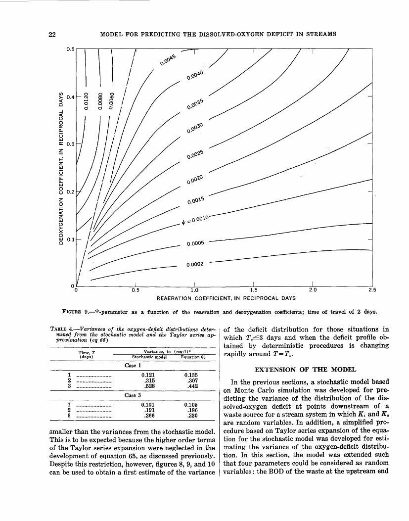
22 MODEL FOR PREDICTING THE DISSOLVED-OXYGEN DEFICIT IN STREAMS

or>.~ o!=S

ooo.O Q.

en >-<( o?J~ Q o9 ..J <( u 0 o?Jo c::: Q.. o9 u LLJ c::: 0.3 z oo~~ t-= Q.

z LLJ

u Li: oo~o LL. LLJ 0· 0 0.2 u z . o\~ 0 o.o i= <( z "-' ::::o.oolO LLJ (.!)

>-X 0 LLJ 0.1 Q 0.0005

0.0002

00~------------~=--------------L---------------L--------------~------------~ 0.5 1.0 1.5 2.0 2.5

REAERATION COEFFICIENT, IN RECIPROCAL DAYS

FIGURE 9.-'l'-parameter as a function of the reaeration and deoxygenation coefficients; time of travel of 2 days.

TABLE 4.-Variances of the oxygen-deficit distributions deter­mined from the stochastic model and the Taylor series ap­proximation ( eq 65)

Time,T Variance, in (mg/1) 2

(days) Stochastic model Equation 65

Case 1

1 ------------ 0.121 0.135 2 ------------ .315 .307 3 ------------ .528 .442

Case 3

1 ------------ 0.101 0.105 2 ------------ .191 .186 3 ------------ .266 .230

smaller than the variances from the stochastic model. This is to be expected because the higher order terms of the Taylor series expansion were neglected in the development of equation 65, as discussed previously. Despite this restriction, however, figures 8, 9, and 10 can be used to obtain a first estimate of the variance

of the deficit distribution for those situations in which TcL3 days and when the deficit profile ob­tained by deterministic procedures is changing rapidly around T=Tc.

EXTENSION OF THE MODEL

In the previous sections, a stochastic model based on Monte Carlo simulation was developed for pre­dicting the variance of the distribution of the dis­solved-oxygen deficit at points downstream of a waste source for a stream system in which K1 and K2 are random variables. In addition, a simplified pro­cedure based on Taylor series expansion of the equa­tion for the stochastic model was developed for esti­mating the variance of the oxygen-deficit distribu­tion. In this section, the model was extended such that four parameters could be considered as random variables: the BOD of the waste at the upstream end

EXTENSION OF THE MODEL 23

en 0.4 >-<( 0 ....J <( u 0 0::: tl. u LiJ 0::: 0.3 z ....: z LiJ

u u:: LL. LiJ 0 0.2 u z 0 ~

0.oo\~ <( z LiJ (.!)

>->< 0

0.1 LiJ 0

00~------------~------------~~----------~~------------~------------_j 0.5 1.0 1.5 2.0 2.5

REAERATION COEFFICIENT, IN RECIPROCAL DAYS

FIGURE 10.-.Y-parameter as a function of the reaeration and deoxygenation coefficients; time of travel of 3 days.

of the reach (Lo), the deoxygenation coefficient at the upstream end of the reach (K1 ), the deoxygena­tion coefficient along the reach (k), and the reaera­tion coefficient (K2). In addition, correlation was assumed between K2 and k and between K1 and L0 •

The fundamental equation of the stochastic model (eq 41) was used with three changes: B was as­sumed negligible, K3 was assumed zero, and the variation of K1 along the reach was separated from the variation of the initial K1 values by the addition of the k parameter. These changes are for the pur­pose of simplification only; they do not in any way change the basic procedures used in the computa­tions. With these changes, equation 41 becomes

~ { K1+k1 D=Lo exp (- L..J K2iaT) i=1 (K21 -Kl-kl)

+ ni:1 (Kl + ki) (K2i+ 1)- (K2i) (Kl + ki+l)

i= 1 (Kzi- K1- k,,) (K2i+l- K1- ki+1)

i exp [ L (K2.-K1-k1)aT]

. 1 J J=

L+~ n } + K .. -K -k exp [ .L (K2j-K1-k1)aT] . (70) ~n 1 n J = 1

Equation 70 permits the computation of the oxy­gen deficit for a specific time T where naT= T and n is the number of steps assumed for the random walk. Repetition of the computations m times then yields m values for the oxygen deficit from which the mean and the variance of the deficit are computed. In a practical situation, however, the time of travel of most importance is the critical time of travel or the time when the deficit is maximum. This is the time at which violations of the quality standards are most likely to occur and hence, the time for which esti­mates of the variance are most necessary. There­fore, in contrast to previous sections where compu­tations were for general times of 1, 2, 3, 4, or 5 days,

24 MODEL FOR PREDICTING THE DISSOLVED-OXYGEN DEFICIT IN STREAMS

calculations in this section will be specifically for the critical time of travel.

However, the critical time of travel for the sto­chastic model cannot be determined explicitly from equation 70, in contrast to the deterministic model for which Tc can be computed. In theory, Tc could be determined by applying the Monte Carlo simulation procedure to sequentially increasing times until the maximum deficit is found. In practice, however, the computer expenses would be prohibitive. Therefore, the procedure used was to compute the variances for the distributions of the deficit for the deterministic Tc, given by

Ten= 1 m/1'!_, [ K2(l- Do(K2-K1) )] (71 ) K2-K1 K1 Lo

and for a stochastic critical time of travel, Tc, ob-s tained from the Taylor series expansion approxima-tion of equation 70. These critical times of travel in general will not be the same; results presented pre­viously suggested that the critical time of travel for the stochastic model was larger than the determin­istic critical time of travel. The procedure used to estimate the stochastic critical time of travel will be described shortly.

MONTE CARLO COMPUTATIONS

The basic Monte Carlo simulation procedure was as described previously and as shown in figures 22, 23, and 24 ; however, because of the several changes in this section, the procedure will be outlined quali­tatively here. Input data consisted of the coefficients of variation of the reaeration coefficient (K2), of the deoxygenation coefficient along the reach ( k) , of the total deoxygenation coefficient (K1 + k), and of the BOD at the upstream end of the reach (Lo) ; the cor­relation coefficients between K1 and Lo and between K2 and k; and the critical time of travel. Steps in the procedure were:

1. Selection of Lo from a normal distribution. 2. Selection of K 1 from a normal distribution with

the specified correlation coefficient between Lo and K1.

3. Selection of K1 +k and K2 to be used in the ran-dom walk computations ( eq 70) .

4. Computation of the oxygen deficit. 5. Repetition of the procedure m times. 6. Computation of the mean and the variance from

them values of the oxygen deficit.

The Monte Carlo computations were completed for 25 sets of K1 and K2 values with the following conditions:

Cv(K1 +k) =0.35

Cv(k) =0.19

Cv (K2) = 0.30

Cv (Lo) = 0.20

r (KH Lo) = -0.67

r(K2, k) =0.50

Lo=l.O mg/1

Do=O

n=100

m = 800 for most computations, 200 for some com-putations.

These conditions were also used in all computations in this section with the Taylor series approximation of the stochastic model.

ESTIMATION OF THE MEAN AND THE VARIANCE OF THE OXYGEN-DEiFICIT DISTRIBUTION

As in previous sections, the mean and the vari­ance of the distribution of the oxygen deficit may be estimated from a Taylor series approximation of the stochastic model. Basically it is assumed that

D = h (K11, K12 , ••• K1,; K21, K22 , ••• K2,; Lo1, Lo2 , ••• Lo,; k~t k2, ... kn). (72)

Expanding in a Taylor series, taking expected values, and assuming correlation only between K1, and Loi and between K2i and ki gives

- - - - var Lo o2h Mean D=h(K~t K2, Lo, k) + -

2 oL2

0

(73)

where var implies variance and P: = f3 1 - /3': •

Determining the derivatives from equation 70, evaluating at the mean values of the variables, and substituting into equation 72 gives

Mean D=h+H1+H2+Ha+H4+Hs (74)

where

(75)

EXTENSION OF THE MODEL 25

- - [ K.l Ha=r(K2, k) ({3~f3)tf2TLoe-K2T 2(K2-Kt)2

(e<il2-il1>T-1)+ K2 (1-e<K2-K1>T)J (78) 2(K2-K1) 2

H4 1 o 2K2 (e<K2-Kt)T-1)- 2KzT {3' L e-K2T[ _ _

2 (K2-Kt) 3 (K2-Kl)2

- - K1T2 J e<Ke-Kt)T + e<K2-K1)T (79)

(K2-Kt)

- - [ K2 H5 =r(K1, L 0 ) ({3:)112LoCv(Lo)e-K~r (K2

-K1)2

(e<K2-Kt)T-l) e(K2-K1)T . - - K1T - - J K2-K1

(80)

The terms HH H2, and Ha represent the effects on the deficit of the variation of the deoxygenation coeffi­cient along the reach, the variation of the reaeration coefficient, and the correlation between these coeffi­cients, respectively; allowing for slight changes in nomenclature and the assumption that Ka = 0 in the present section, H H H 2, and H a are equivalent to G1, G2, and Ga (eqs 59, 60, and 61), respectively. The terms H4 and Hs represent the effect on the deficit of the variation of the initial value of the deoxygena­tion coefficient and the correlation between the ini­tial deoxygenation coefficient and upstream BOD, respectively. Variations in the upstream BOD do not affect estimates of the mean deficit because o2h/0L 2 =0. When the variables K1.,K2., Lo., and ki

0 ~ t t

are assumed independent of time of travel, then H 1,

H 2, H a, H4, and H s are zero and equation 73 reduces to

Mean D=h (81)

or the classical oxygen sag equation of Streeter and Phelps (1925) (see eq 4).

By similar arguments, it may be shown that

n T h n T h Var D=/3" L - (~)2+,82 L-(-0

-)'2 1 i=l D..T ok1 .i=tAT oK2i

n +2r(K2, k) ({3"{3 )1/2 L _!__ (~) ( oh )

1 2 i=l aT oK2i oki

+ Var Lo ( oLh )2 + {3' ( oKh ) 2

0 0 1 0 1

+2r(KH Lo) ({3' var Lo)112 ( oh )( oh ). (82) 1 oK1 oLo

Evaluating derivatives as before, it follows that

Var D=Hs+H1+Hs+H9+H1o+Hn (83)

where

( e•(K,-l!',l 7' -e<K,-lM7') J (89)

The terms H 6' H 1' and H s represent the effects on the variance of the distribution of the deficit of the

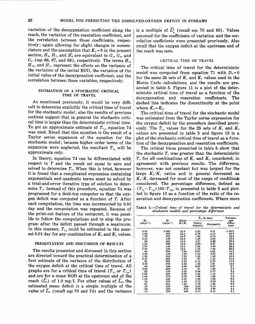
26 MODEL FOR PREDICTING THE DISSOLVED-OXYGEN DEFICIT IN STREAMS

variation of the deoxygenation coefficient along the reach, the variation of the reaeration coefficient, and the correlation between these coefficients, respec­tively; again allowing for slight changes in nomen­clature and the assumption that K 3 = 0 in the present section, H6, H7, and H 8 are equivalent to G4, G5 , and G6 (eqs 66, 67, and 68), respectively. The terms H 9 ,

H1o, and H11 represent the effects on the variance of the variation of the initial BOD, the variation of the initial value of the deoxygenation coefficient, and the correlation between these variables, respectively.

ESTIMATION OF A STOCHASTIC CRITICAL TIME OF TRAVEL

As mentioned previously, it would be very diffi­cult to determine explicitly the critical time of travel for the stochastic model ; also the results of previous sections suggest that in general the stochastic criti­cal time is larger than the deterministic critical time. To get an approximate estimate of Tcs' equation 7 4 was used. Recall that this equation is the result of a Taylor series expansion of the equation for the stochastic model; because higher order terms of the expansion were neglected, the resultant Tc

8 will be

approximate only.

In theory, equation 7 4 can be differentiated with respect to T and the result set equal to zero and solved to determine Tc. When this is tried, however it is found that a complicated expression containing exponentials and quadratic terms must be solved by a trial-and-error iterative type of solution to deter­mine Tc. Instead of this procedure, equation 74 was programed for a desk-top computer so that the oxy­gen deficit was computed as a function of T. After each computation, the time was incremented by 0.01 day and the computation was repeated. Because of the print-out feature of the computer, it was possi­ble to follow the computations and to stop the pro­gram after the deficit passed through a maximum. In this manner, Tc

8 could be estimated to the near­

est 0.01 day for any combination of K1 and K2 values.

PRESENTATION AND DISCUSSION OF RESULTS

The results presented and discussed in this section are directed toward the practical determination of a first estimate of the variance of the distribution of the oxygen deficit at the critical time of travel. All graphs are for a critical time of travel (Tc

8 or Tcv)

and are for a mean BOD at the upstream end of the reach (Lo) of 1.0 mg/1. For other values of Lo, the estimated mean deficit is a simple multiple of the value of Lo (recall eqs 70 and 7 4) and the variance

is a multiple of L 2 (recall eqs 70 and 83). Values I)

assumed for the coefficients of variation and the cor-relation coefficients were presented previously. Also recall that the oxygen deficit at the upstream end of the reach was zero.

CRITICAL TIME OF TRAVEL

The critical time of travel for the deterministic model was computed from equation 71 with Do= 0 for the same 25 sets of K1 and K2 values used in the Monte Carlo calculations, and the results are pre­sented in table 5. Figure 11 is a plot of the deter­ministic critical time of travel as a function of the deoxygenation and reaeration coefficients. The dashed line indicates the discontinuity at the point where K1 =K2.

The critical time of travel for the stochastic model was estimated from the Taylor series expression for the oxygen deficit by the procedure described previ­ously. The Tcs values for the 25 sets of K1 and K2 values are presented in table 5 and figure 12 is a plot of the stochastic critical time of travel as a func­tion of the deoxygenation and reaeration coefficients.

The critical times presented in table 5 show that the stochastic Tc was greater than the deterministic Tc for all combinations of K1 and K2 considered, in agreement with previous results. The difference, however, was not constant but was largest for the large KdK1 ratios and in general decreased _as K 2/K1 decreased for most of the range of conditior.is considered. The percentage difference, defined as (Tc

8-Tcv)100/Tc,n' is presented in table 5 and plot-

ted in figure 13 as a function of the ratio of the re­aeration and deoxygenation coefficients. Where more

TABLE 5.-Critical time of travel for the deterministic a11.d stochastic models and percentage difference

Tc, in days Percent-K2 K1 Ratio age

(days-1 ) (days-1 ) K2/K1 Deter- Stochastic differ-ministic ence

0.60 0.025 24.0 5.53 8.21 +48.5 1.20 .050 24.0 2.76 4.10 48.6 1.80 .075 24.0 1.84 2.74 48.9 2.40 .100 24.0 1.38 2.05 48.6 .60 .045 13.3 4.67 5.9.0 26.3

1.20 .095 12.6 2.30 2.87 24.8 1.80 .140 12.9 1.54 1.93 25.3 2.40 .190 12.6 1.15 1.44 25.2

.60 .080 7.60 3.87 4.50 16.3 1.20 .160 7.50 1.94 2.25 16.0 1.80 .240 7.50 1.29 1.50 16.3 2.40 .320 7.50 .97 1.13 16.5

.40 .075 5.33 5.15 5.78 12.2 2.00 .375 5.33 1.03 116 12.6 .40 .100 4.00 4.62 5.07 9.7

2.05 .500 4.10 .91 1.00 9.9 .50 .150 3.33 3.44 3.73 8.4

1.65 .500 3.30 1.04 1.13 8.7 1.00 .370 2.70 1.58 1.69 7.0 1.00 .445 2.25 1.46 1.55 6.2

.50 .259 1.93 2.73 2.89 5.9

.80 .415 1.93 1.70 1.80 5.9

.30 .375 .800 2.98 3.10 4.0

.20 .325 .615 3.88 4.05 4.4

.10 .250 .400 6.10 6.41 5.1

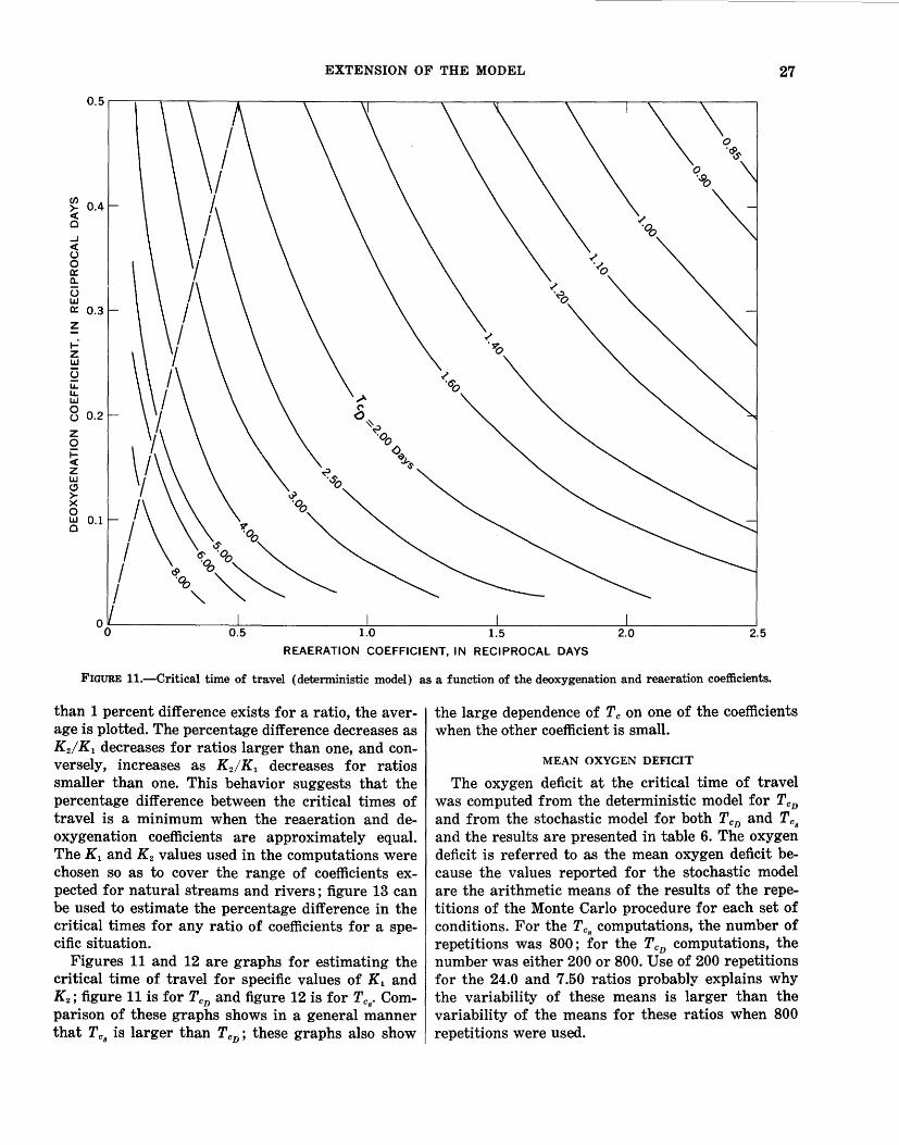
EXTENSION OF THE MODEL 27

ffJ 0.4 >-<( Cl

...J <( (.)

0 0:: ll.

u IJ.I 0:: 0.3 z r= z IJ.I

u u:: LL IJ.I 0 0.2 (.)

z 0 i= <( z IJ.I (!)

>-X 0 IJ.I Cl

0.1

00~------------~~------------~--------------~--------------~------------~ 0.5 1.0 1.5 2.0 2.5

REAERATION COEFFICIENT, IN RECIPROCAL DAYS

FIGURE 11.-Critical time of travel (deterministic model) as a function of the deoxygenation and reaeration coefficients.

than 1 percent difference exists for a ratio, the aver­age is plotted. The percentage difference decreases as K2/K1 decreases for ratios larger than one, and con­versely, increases as K2/K1 decreases for ratios smaller than one. This behavior suggests that the percentage difference between the critical times of travel is a minimum when the reaeration and de­oxygenation coefficients are approximately equal. The K1 and K2 values used in the computations were chosen so as to cover the range of coefficients ex­pected for natural streams and rivers; figure 13 can be used to estimate the percentage difference in the critical times for any ratio of coefficients for a spe­cific situation.

Figures 11 and 12 are graphs for estimating the critical time of travel for specific values of K1 and K2; figure 11 is for Ten and figure 12 is for Tcs· Com­parison of these graphs shows in a general manner that Tc

8 is larger than Ten; these graphs also show

the large dependence of T c on one of the coefficients when the other coefficient is small.

MEAN OXYGEN DEFICIT

The oxygen deficit at the critical time of travel was computed from the deterministic model for TeD

and from the stochastic model for both T cD and T c8

and the results are presented in table 6. The oxygen deficit is referred to as the mean oxygen deficit be­cause the values reported for the stochastic model are the arithmetic means of the results of the repe­titions of the Monte Carlo procedure for each set of conditions. For the Tc

8 computations, the number of

repetitions was 800; for the TeD computations, the number was either 200 or 800. Use of 200 repetitions for the 24.0 and 7.50 ratios probably explains why the variability of these means is larger than the variability of the means for these ratios when 800 repetitions were used.

28 MODEL FOR PREDICTING THE DISSOLVED-OXYGEN DEFICIT IN STREAMS

~a v C/)

0.4 >-< 0 ....J < (.)

0 0::: a. u IJ.I 0::: 0.3 z ..: z IJ.I

u -" u: (' u.. .r IJ.I ~ 0 0.2 ~a (.) Db z q..J..-s 0 i= < z IJ.I C!J >-X 0 IJ.I 0.1 0

0o~------------~o~.5--------------~1~.o--------------~1~.5~------------~2~.o~------------~2.5

REAERATION COEFFICIENT, IN RECIPROCAL DAYS

FrGURE 12.-Critical time of travel (stochastic model) as a function of the deoxygenation and reaeration coefficients.

The oxygen deficits are plotted in figure 14 as a TABLE 6.-Mean oxygen deficit for deterministic and stochastic

function of the ratio of the reaeration and deoxy- models

genation coefficients. The results in figure 14 and Mean oxygen deficit, in mg/1

table 6 show that the oxygen deficit for the deter- K2 K1 Ratio Deter- Sto- Sto-(days-1 ) (days-1 ) K2/K1 minis tic chastic chastic

mini.stic model tends to be slightly larger than the TeD TeD Tc,

deficit for the stochastic model for small ratios, but 0.60 0.025 24.0 0.0363 0.0343 0.0380

in general the differences among the oxygen deficits 1.20 .050 24.0 .0363 .0362 .0380 1.80 .075 24.0 ,().363 .0377 .0380

are negligible. Also, the relatively large difference in 2.40 .100 24.0 .0363 .0388 .0380 .60 .045 13.3 .0608 .0632 .0625

Tc8

and Ten for large ratios had relatively little effect 1.20 .095 12.6 .0637 .0644 .0647 1.80 .140 12.9 .0627 .0651 .0628

on the computation of the deficit by the stochastic 2.40 .190 12.6 .0637 .0641 .0653 .60 .080 7.50 .0978 .0962 .0970

model. 1.20 .160 7.50 .0978 .0968 .0975 1.80 .240 7.50 .0978 .0944 .0996 2.40 .320 7.50 .0978 .0898 .100

The oxygen deficit was also computed from the .40 .075 5.33 .127 .122 .127 2.00 .375 5.33 .127 .125 .121

Taylor series approximation (recall eq 73) for Tc8

.40 .100 4.00 .158 .153 .152 2.05 .500 4.10 .155 .148 .153

and the results are presented in table 7 together with .50 .150 3.33 .179 .162 .172 1.65 .500 3.30 .180 .171 .176

stochastic model results for Tc . The oxygen deficits 1.00 .370 2.70 .206 .195 .200 8 1.00 .445 2.25 .232 .219 .223

are plotted in figure 15 as a function of the ratio of .50 .259 1.93 .256 .225 .245 .80 .415 1.93 .256 .242

the reaeration and deoxygenation coefficients. The .30 .375 .800 .410 .382 .386 .20 .325 .615 .460 .436

results show that the oxygen deficits computed for .10 .250 .400 .543 .506 .507

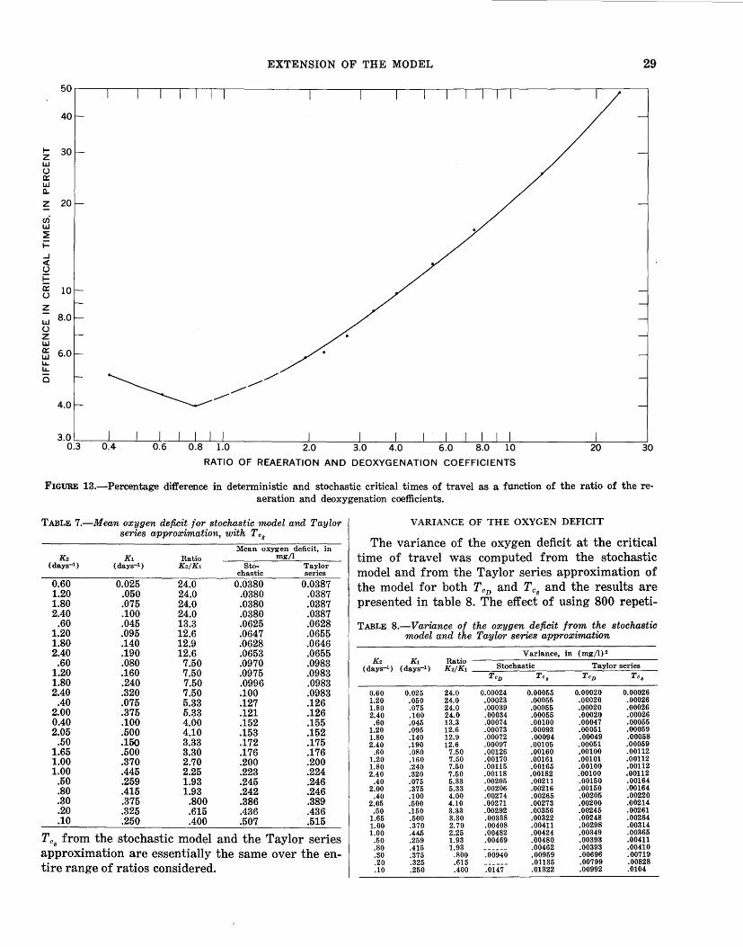
EXTENSION OF THE MODEL 29

50

40

1- 30 z LLJ (.) 0::: LLJ a.. z 20

u) LLJ ~ i= ....J < (.)

E 0::: (.)

z LLJ (.) z LLJ 0::: LLJ LL. LL.

Q

~---------./ 4.0

3.0 0.3 20 30

RATIO OF REAERATION AND DEOXYGENATION COEFFICIENTS

FIGURE 13.-Percentage difference in deterministic and stochastic critical times of travel as a function of the ratio of the re-aeration and deoxygenation coefficients.

TABLE 7.-Mean oxygen deficit for stochastic model and Taylor VARIANCE OF THE OXYGEN DEFICIT series approxinnation, with T c

8 The variance of the oxygen deficit at the critical

Mean oxygen deficit, in K2 K1 Ratio mg/1 time of travel was computed from the stochastic

(days-1) (days-1) K2/K1 Sto- Taylor model and from the Taylor series approximation of chastic series

0.60 0.025 24.0 0.0380 0.0387 the model for both Tcv and Tc8

and the results are 1.20 .050 24.0 .0380 .0387 1.80 .075 24.0 .0380 .0387 presented in table 8. The effect of using 800 repeti-2.40 .100 24.0 .0380 .0387

.60 .045 13.3 .0625 .0628 TABLE B.-Variance of the oxygen deficit from the stochastic 1.20 .095 12.6 .0647 .0655 model and the Taylor series approximation 1.80 .140 12.9 .0628 .0646 2.40 .190 12.6 .0653 .0655 Variance, in (mg/1) 2

.60 .080 7.50 .0970 .0983 K2 K1 Ratio Stochastic Taylor series (days-1 ) (days-1 ) K2/K1 1.20 .160 7.50 .0975 .0983 TeD Tc 8 TeD Tc 8 1.80 .240 7.50 .0996 .0983

2.40 .320 7.50 .100 .0983 0.60 0.025 24.0 0.00024 0.00055 0.00020 0.00026

.40 .075 5.33 .127 .126 1.20 .050 24.0 .00023 .00055 .00020 .00026 1.80 .075 24.0 .00039 .00055 .00020 .00026 2.00 .375 5.33 .121 .126 2.40 .100 24.0 .00034 .(}0055 .00020 .00026

0.40 .100 4.00 .152 .155 .6(} .045 13.3 .00074 .00100 .00047 .00055

2.05 .500 4.10 .153 .152 1.20 .095 12.6 .00073 .00093 .00051 .00059 1.80 .140 12.9 .0(}072 .00094 .00049 .00058

.50 .150 3.33 .172 .175 2.40 .190 12.6 .00097 .00105 .00051 .00059 1.65 .500 3.30 .176 .176 .60 .080 7.50 .00126 .00160 .00100 .00112

1.00 .370 2.70 .200 .200 1.20 .160 7.50 .00170 .00161 .00101 .00112 1.80 .240 7.50 .00115 .00165 .00100 .00112

1.00 .445 2.25 .223 .224 2.40 .320 7.50 .00118 .00182 .00100 .00112 .50 .259 1.93 .245 .246 .40 .075 5.33 .00205 .00211 .00150 .00164

.80 .415 1.93 .242 .246 2.00 .375 5.33 .00206 .00216 .00150 .00164 .40 .100 4.00 .00274 .00265 .00205 .00220

.30 .375 .800 .386 .389 2.05 .500 4.10 .00271 .00273 .00200 .00214

.20 .325 .615 .436 .436 .50 .150 3.33 .00292 .00356 .00245 .00261

.10 .250 .400 .507 .515 1.65 .500 3.30 .00338 .00322 .00248 .00264 1.0(} .370 2.70 .00408 .00411 .00298 .00314

Tc8

from the stochastic model and the Taylor series 1.00 .44,5 2.25 .00482 .00424 .00349 .00365 .50 .259 1.93 .00469 .00480 .00393 .00411

approximation are essentially the same over the en- .80 .415 1.93 .00462 .00393 .00410 .30 .375 .800 .00940 .00959 .00696 .00'719

tire range of ratios considered. .20 .325 .615 .01135 .00799 .00828 .10 .250 .400 .0147 .01322 .00992 .0104

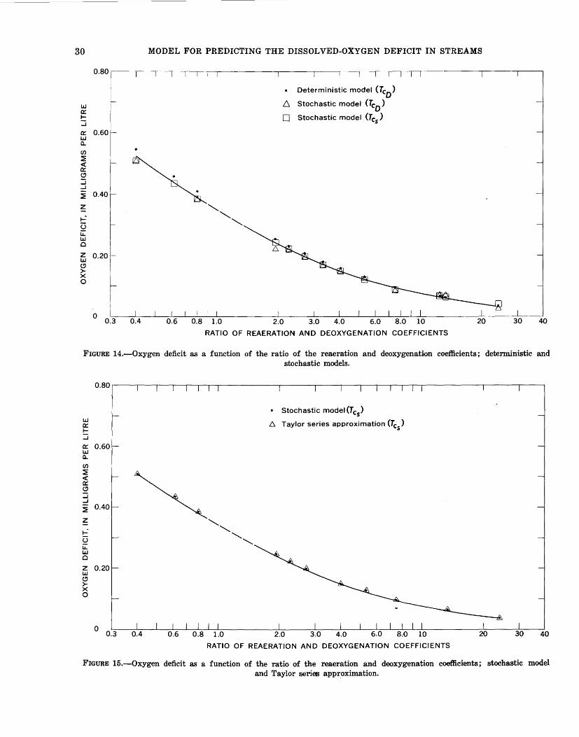
30

LIJ 0::: ..... :::i 0::: 0.60 LIJ a.. rn ~ <( 0::: <!)

:::i ...J

~ 0401 t-=" u i:L: LIJ 0

~ 0.20 <!) >­X 0

MODEL FOR PREDICTING THE DISSOLVED-OXYGEN DEFICIT IN STREAMS

Deterministic model (Te0

> 6 Stochastic model (Te

0)

D Stochastic model (Te5

)

RATIO OF REAERATION AND DEOXYGENATION COEFFICIENTS

FIGURE 14.-0xygen deficit as a function of the ratio of the reaeration and deoxygenation coefficients; detenn.inistic and stochastic models.

• Stochastic model (Te5

)

LIJ 0::: t::

!:::.. Taylor series approximation (Te5

)

...J

0::: LIJ a.. rn ~ <( 0::: <!)

:::i ...J

~ 0.40

z t-=" C3 i:L: LIJ 0

z 0.20 LLI <!)

>-X 0

0 0.3 4.0 20 40

RATIO OF REAERATION AND DEOXYGENATION COEFFICIENTS

FIGURE 15.-0xygen deficit as a function of the ratio of the reaeration and deoxygenation coefficients; stochastic model and Taylor seriE!IS approximation.

EXTENSION OF THE MODEL 31

tions in the computations for the stochastic model with Tc

8 as compared with 200 repetitions for Ten is

again noticeable, particularly for the 24.0 and 7.50 ratios. The variability of the variances within a group is much larger for the calculations with 200 repetitions. It is also interesting that the largest variances for the 7.50 ratio occurred for different combinations of K2 and K1. This probably occurs be­cause of the random nature of the simulation process.

The variances computed from the stochastic model and the Taylor series approximation with the deter­ministic critical time of travel are plotted in figure 16 as a function of the ratio of the reaeration and

·deoxygenation coefficients. The average variance was plotted for those ratios where several variances were computed. The variance from the stochastic model is larger than the variance from the Taylor series approximation over the entire range of ratios considered. This difference undoubtedly occurred because higher order terms in the Taylor series ex­pansion were neglected. Figure 16 also shows the random nature of the simulation process in that the points for the stochastic model tend to scatter about the trend line whereas the points for the Taylor series approximation all tend to lie on the trend line.

The variances computed with the stochastic criti-

0.0150·-~~~~~~~~~~~~~~---~~~~~~~~~~~~~~~~--~--~--~-.

0.0100

0.0060

"' 0.0040 UJ c::: 1-:::i c::: LLI a.. en ::?! <( 0.0020 c::: (.!)

::::i ...J

::?!

~ u.i (.) 0.0010 z ~ c::: 0.0008 <(

>

0.0006

0.0004

. !::::.

""­"-. .........

Stochastic model (Te0>

Taylor series approximation (Te0>

RATIO OF REAERATION AND DEOXYGENATION COEFFICIENTS

l

FIGURE 16.-Variance of the oxygen deficit as a function of the ratio of the reaeration and deoxygenation coefficients; stochastic model and Taylor series approximation with the deterministic critical time of travel.

32 MODEL FOR PREDICTING THE DISSOLVED-OXYGEN DEFICIT IN STREAMS

cal time of travel are plotted in figure 17 as a func­tion of the ratio of the reaeration and deoxygena­tion coefficients. The dependence of the variance on the ratio is essentially identical to the behavior for the deterministic critical time of travel shown in figure 16, with the exception that the curve for the Taylor series approximation falls away more rapid­ly than the stochastic model curve for large ratio values.

The effect on the variance of the type of critical travel time used in the computations is shown in figures 18 and 19. Figure 18 shows the variation

(\1

w a:: 1-:::i a:: UJ a.. C/)

~

0.0100

0.0060

~ 0.0020 ~ :::i ...J

~ ~ w () z ct a:: ct 0.0008 >

0.0006

0.0005 • Stochastic model (Tc5

)

with the ratio of the reaeration and deoxygenation coefficients of the variance computed from the sto­chastic model; figure 19 shows the variation with the ratio of the coefficients of the variance computed from the Taylor series approximation. Figure 18 shows that the variances are essentially identical for the two critical times up to a ratio of about 4 at which point the variances computed for Ten drop off more rapidly than the variances computed for Tc

8•

Figure 19 shows essentially the same behavior for the Taylor series approximation except that there is less scatter of the points around the curves. Also the

0.0004 D,. Taylor series approximation (Tc

5)

0.0003

RATIO OF REAERATION AND DEOXYGENATION COEFFICIENTS

FIGURE 17.-Variance of the oxygen deficit as a function of the ratio of the reaeration and deoxygenation coefficients; stochastic model and Taylor series approximation with the stochastic critical time of travel.

EXTENSION OF THE MODEL 33

0.0150r----~~~-,--.-.--,-,~l-----------,----~----.---~.--,~-,l-.l-----------~-----

N

w a::: 1-:::i a::: L&J c.. CJ)

~ <t a::: (.!)

:::i ...J

~ z u.i (.)

z ~ a::: <t >

0.0080

0.0060

0.0006

0.0003

"'-.. "'-..

Stochastic model

0.0002~~~~~~~~~--------~~--~~--~--~~--~~~~--------~----~ 0.3 0.4 1.0 6.0 20 30

RATIO OF REAERATION AND DEOXYGENATION COEFFICIENTS

FIGURE 18.-Variance of the oxygen deficit as a function of the ratio of the reaeration and deoxygenation coefficients; stochastic model with the deterministic and stochastic critical times of travel.

Tc8

results are always larger than the TeD results and the difference increases as the ratio of the reaeration and deoxygenation coefficients increases, in agree­ment with the dependence of the difference of the critical times of travel on the ratio (recall fig. 13). Consideration of figures 13, 18, and 19 suggests that the variance for a specific set of conditions tends to increase as the estimate of the critical time of travel increases and the amount of the increase increases as the ratio of the coefficients increases. This ob­servation is qualitatively in agreement with the re­sults of the analysis of the Sacramento River data where it was concluded that the variance was a maxi-

mum for some time larger than the critical time of travel.

The ·Taylor series expression for the variance (re­call eq 83) may be used to determine the relative contributions of the various terms to the total vari­ance. The terms H 6' H 1, H a, H 9' H 10, and H 11 were computed for each of the sets of reaeration and de­oxygenation coefficients (see table 5) with Tc

8 and

the other coefficients given previously. The results are presented in table 9. Because the results were the same for each ratio of K2 and K1, only one result for each ratio is given in table 9. Recall that H6, H1, and H 8 represent the effects on the variance of the varia-

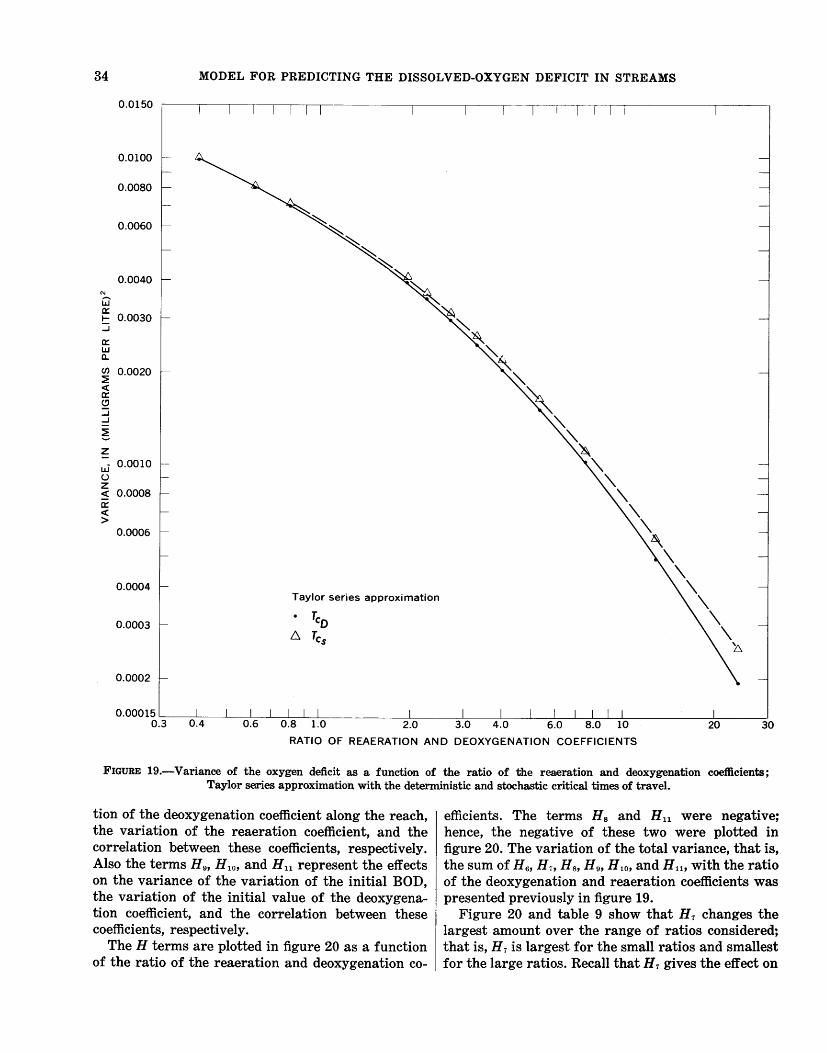
34 MODEL FOR PREDICTING THE DISSOLVED-OXYGEN DEFICIT IN STREAMS

0.0150

0.0100

0.0080

0.0060

0.0040 C\1

w 0:: t:: 0.0030 ..J

0:: UJ Q..

C/) 0.0020 ~ <( 0:: (.!J

:::i ..J

~ z ~ 0.0010 -(.)

z ~ 0.0008 0:: <(

> 0.0006

0.0004

0.0003

0.0002

Taylor series approximation

• Teo

!::::. Tcs

0.6 0.8 1.0

RATIO OF REAERATION AND DEOXYGENATION COEFFICIENTS

20 30

FIGURE 19.-Variance of the oxygen deficit as a function of the ratio of the reaeration and deoxygenation coefficients; Taylor series approximation with the deterministic and stochastic critical times of travel.

tion of the deoxygenation coefficient along the reach, the variation of the reaeration coefficient, and the correlation between these coefficients, respectively. Also the terms H 9' H 10, and H 11 represent the effects on the variance of the variation of the initial BOD, the variation of the initial value of the deoxygena­tion coefficient, and the correlation between these coefficients, respectively.

The H terms are plotted in figure 20 as a function of the ratio of the reaeration and deoxygenation co-

efficients. The terms Hs and Hn were negative; hence, the negative of these two were plotted in figure 20. The variation of the total variance, that is, the sum of H 6' H ,, H s, H 9' H 1o, and H n, with the ratio of the deoxygenation and reaeration coefficients was presented previously in figure 19.

Figure 20 and table 9 show that H 1 changes the largest amount over the range of ratios considered; that is, H 1 is largest for the small ratios and smallest for the large ratios. Recall that H 1 gives the effect on

EXTENSION OF THE MODEL 35

TABLE 9.-Distribution of the variance among the terms making up the variance estimated by the Taylor series approxima­tion of the stochastic model

H terms, in (milligrams per litre) 2 Variance

t::: (.)

Li: LLJ 0

z LLJ (.!)

?<~ QLLJ

0::: 1.&..1-0::J Ll.lo::: Uw ~0.. -C/) 0:::~ ~<( LLJO:: :I:~ 1-j

24.0 12.9 7.50 5.33 4.00 3.33 2.70 2.25 1.93

.800

.615

.400

0.01000

0.00100-

0.00040

H6

0.0000744 .000212 .000464 .000718 .000997 .00120 .00147 .00171 .00191 .00282 .00288 .00269

H1 Hs

0.0000493 -0.0000812 .000153 -.000241 .000376 -.000560 .000642 -.000910 .000985 -.00133 .00128 -.00166 .00170 -.00211 .00215 -.00257 .00260 -.00299 .00670 -.00582 .00844 -.00660 .0118 -.00753

o..-:::> ~ 0.00020

(.!)z z-::s::: <( ~ C/)

~ 0::: LLJ 1-

0.00010

0.00006

0.00004 ~-----=-'--=---'---c:~~LLLL__ _ _l_____j_____L__jl__l_LL.l__L__J___)

0.1 0.2 0.4 0.6 1.0 2.0 4.0 6.0 10 20 30

RATIO OF REAERATION AND DEOXYGENATION COEFFICIENTS

FIGURE 20.-Distribution of the variance among the terms making up the variance as a function of the ratio of the reaeration and deoxygenation coefficients.

the variance of random variations in the reaeration coefficient. Thus, in a deep, slow-flowing stream with a small reaeration coefficient, random variations in K2 make the largest contribution to the variance of the oxygen deficit. On the other hand, for a shallow, rapidly flowing stream with a large reaeration coeffi­cient and the same deoxygenation coefficient, random variations in K2 make the smallest contribution to the variance of the oxygen deficit. This difference in contribution may also be seen by computing the per­centage of the total variance that each of the six terms contributes. For KdK1 = 24.0, the percentages are 29.1, 19.3, -31.7, 38.7, 109.4, .and -64.8 for H6, I H1, Hs, H9, H1o, and Hn, respectively; for KdK1 =

Ho H1o Hn (mg/1)2

0.0000990 0.000280 -0.000166 0.000256 .000208 .000599 -.000352 .000579 .000383 .00111 -.000650 .00112 .000544 .00157 -.000921 .00164 .000710 .00203 -.00120 .00219 .000827 .00236 -.00140 .00261 .000971 .00275 -.00163 .00315 .00110 .00310 -.00184 .00365 .00120 .00340 -.00202 .00410 .00161 .00460 -.00272 .00719 .00162 .00470 -.00275 .00829 .00148 .00454 -.00259 .0104

0.400, the percentages are 25.9, 113.6, -72.5, 14.2, 43.7, and -24.9, respectively. Thus, the contribution of H1 increases from 19.3 percent to 113.6 percent as K2/K1 decreases from 24.0 to 0.400.

Figure 20 and table 9 show that H6, H9, H1o, and H n all have maximum contributions to the variance at a ratio of 0.615 for the specific values of ratios considered. However, for ratios between 0.4 and about 2, these four factors do not change appreci­ably. Also, as the ratio decreases, the dependence of the total variance on the ratio decreases (see fig. 19).

· Recall that H11, H 9 , H10 , and Hn give the effect on the variance of random variations in k, random varia­tions in Lo, random variations in KlJ and correlation between Lo and k, respectively.

Figure 20 shows that H9 contributes the least to the total variance over most of the ratio range con­sidered. On the other hand, H 10 contributes the most to the total variance for ratios larger than 1.0. Thus, of the two factors describing the waste at the up­stream end of the reach, the variations in the deoxy­genation coefficient, KlJ contribute the greater amount to the total variance.

Figure 20 shows that the six terms are most near­ly equal in the middle part of the range of ratios considered, that is, between ratios of about 2 and 6. For larger and smaller ratios, the values of the dif­ferent terms diverge. However, for all ratios con­sidered, all the terms contribute significantly to the total variance with the minimum contribution being the 19.3 percent of Hi for a ratio of 24.0.

In considering the results presented in table 9 and figure 20, it should be remembered that these re­sults are specifically only for the values of the co­efficients of variation and the correlation coefficients used in the computations. For other values of these coefficients, the distribution of the total variance among the six terms would undoubtedly be different.

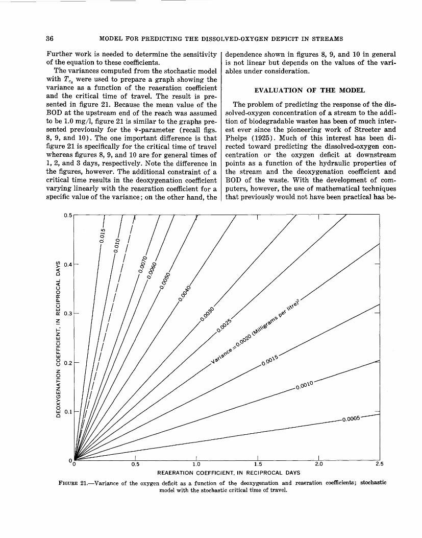
36 MODEL FOR PREDICTING THE DISSOLVED-OXYGEN DEFICIT IN STREAMS

Further work is needed to determine the sensitivity of the equation to these coefficients.

The variances computed from the stochastic model with Tc

8 were used to prepare a graph showing the

variance as a function of the reaeration coefficient and the critical time of travel. The result is pre­sented in figure 21. Because the mean value of the BOD at the upstream end of the reach was assumed to be 1.0 mg/1, figure 21 is similar to the graphs pre­sented previously for the '1!-parameter (recall figs. 8, 9, and 10). The one important difference is that figure 21 is specifically for the critical time of travel whereas figures 8, 9, and 10 are for general times of 1, 2, and 3 days, respectively. Note the difference in the figures, however. The additional constraint of a critical time results in the deoxygenation coefficient varying linearly with the reaeration coefficient for a specific value of the variance; on the other hand, the

~ 0.4 < Cl ...J < u 0 0::: a.. t5 w 0::: 0.3 z ..... -z w t5 u: LL. w 8 0.2

z 0 t= < z w (.!)

> X 0 w 0.1 Cl

0.5 1.0

dependence shown in figures 8, 9, and 10 in general is not linear but depends on the values of the vari­ables under consideration.

EVALUATION OF THE MODEL

The problem of predicting the response of the dis­solved-oxygen concentration of a stream to the addi­tion of biodegradable wastes has been of much inter­est ever since the pioneering work of Streeter and Phelps ( 1925). Much of this interest has been di­rected toward predicting the dissolved-oxygen con­centration or the oxygen deficit at downstream points as a function of the hydraulic properties of the stream and the deoxygenation coefficient and BOD of the waste. With the development of com­puters, however, the use of mathematical techniques that previously would not have been practical has be-

0.ooo5

1.5 2.0 2.5

REAERATION COEFFICIENT, IN RECIPROCAL DAYS

FIGURE 21.-Variance of the oxygen deficit as a function of the deoxygenation and reaeration coefficients; stochastic model with the stochastic critical time of travel.

EVALUATION OF THE MODEL 37

come common. With these techniques, it has become possible to predict the variances of the oxygen deficit and the biochemical-oxygen-demand, in addition to the mean values, at downstream points. This ability adds a new dimension to water-quality standards in that it is possible to estimate the confidence limits for the mean oxygen deficit and hence the proba­bility of failing to meet the standard by any speci­fied amount.

The stochastic model of this study uses Monte Carlo simulation in which a complex system with random components is operated by random numbers chosen so that they simulate the physical behavior of the components. The distribution of the dissolved­oxygen deficit and consequently the mean and vari­ance of the distribution are estimated by repeating the process a large number of times. The model has the capability of considering the reaeration and de­oxygenation coefficients and the BOD at the up­stream end of the reach as random variables; in ad­dition, correlation between pairs of these variables can be considered in the model. The model does not require actual measurements of the variance for pre­diction of other variances, as does the model of Thay­er and Krutchkoff ( 1966). However, considerable information is needed. For each coefficient consid­ered to be a random variable, the variance and the mean value, or equivalently, the coefficient of varia­tion, must be known. For each pair of variables for which correlation is assumed, the correlation coeffi­cient must be known.

Information of this type for the most part is not available; it was necessary to assume values for the coefficients of variation of the reaeration and deoxy­genation coefficients and for the correlation coeffi­cient between these variables for the test of the model with the Sacramento River data. The values assumed, however, were derived from data on other rivers; the coefficient of variation of the deoxygena­tion coefficient was determined from the Ohio River data and the coefficient of variation of the reaeration coefficient was estimated from data for Tennessee Valley streams. The value used for the correlation coefficient was arbitrarily assumed. Consideration of the physical processes involved in the reaeration and deoxygenation process suggests that a positive cor­relation would be expected but gives no indication of the magnitude of the coefficient. It is well known that the deoxygenation and reaeration coefficients deter­mined for one stream or one particular reach of a stream should be used for other streams or other reaches only with caution because of the sensitivity of these coefficients to changes in conditions. But

note that in this instance it is the variability of the coefficients with respect to the mean values that is transferred between streams rather than the mean values. Thus, the assumption is that variations in the coefficients of variation for different streams will be considerably less than variations in the mean values. This assumption is supported by the data for the Tennessee Valley rivers presented in table 11. Note that the reaeration coefficients vary over about a 22-fold range, whereas the coefficients of variation vary only over about a 6-fold range.

The tests of the stochastic model with the hypo­thetical examples, the Sacramento River data, and the computations of the variances at the critical time of travel for the most part gave reasonable values for the variance of the oxygen deficit. This result suggests that the values assumed for the coefficients of variation and the correlation coefficients were reasonable~

As discussed in the previous section, the stochastic model also has the capability of handling the division of random variations in the deoxygenation coeffi­cient between those of the coefficient at the upstream end of the reach and those of the coefficient along the reach. The variances of these two coefficients may be significantly different, as the analysis of the Ohio River data showed; furthermore this differ­ence may significantly affect the calculation of the variance of the deficit distribution. The stochastic model in general can consider any coefficient as a normally distributed random variable if the mean and variance are known; additionally, correlation between any two variables can be treated if the cor­relation coefficient is known. The problem is the de­termination of the coefficients of variation and the correlation coefficients for the variables of interest. Further work in this area is needed.

Comprehensive studies of water quality usually require segmenting the stream when conditions change appreciably with distance downstream. In segmenting, the conditions at the downstream end of each segment serve as the input conditions to the next segment. The stochastic model can be used in this situation, however, a small modification is needed. Recall that in the development of the basic equation of the stochastic model, equation 41, it was assumed that the variance of the initial dissolved­oxygen deficit, Cs-F(~), was small. With segment­ing, this assumption is probably valid only for the first segment because in reality it is the variance of this term, C.y- F (~), which the stochastic model esti­mates for the downstream end of each reach. Hence, the input deficit to the next reach (or segment) is a

38 MODEL FOR PREDICTING THE DISSOLVED-OXYGEN DEFICIT IN STREAMS

random variable with some variance that cannot be neglected. This modification requires that C8 -F(') be removed from the B factor (recall equation 40) and added to the right hand side of equation 41 as

n the term[C8 -F(')] exp (- L K2iD.T).

i=1 Another approach that could be used in applying

the stochastic model to a segmented stream is to use equations 42, 43, 44, and 45. These difference equa­tions segment the stream at D.T intervals and there­fore could be used recurrently in the computation procedure, as described previously. Similarly, the Taylor series approximations of the stochastic mod­el could be applied readily to a segmented stream system.

The basic equation of the stochastic model can be expanded in a Taylor series to give an approximate equation for the variance. This equation involves sums and differences of exponentials and can be solved without a computer; the Monte Carlo com­putations, on the other hand, can be done efficiently only on a computer. It is possible to prepare charts for estimating the variance (recall figs. 8, 9, 10, and 21); these, however, are for specific conditions. Thus, in the event that a preliminary estimate of the variance is desired for conditions not covered by the available charts, the approximate equation may be used. The approximate equation may also be used to indicate how the variance is divided among the various terms describing the total variance, as described previously.

The stochastic model is a step toward the fulfill­ment of the need for a procedure for predicting the variances, in addition to the mean values, of the bio­chemical-oxygen-demand and the dissolved-oxygen deficit at points in a stream downstream from a waste source. Further work is needed, however, on both the experimental and theoretical aspects of the problem. Experimental aspects needing further study are the:

1. Coefficients of variation of the various coefficients and the dependence, if any, on the type of stream.

2. Correlation coefficients between the reaeration and deoxygenation coefficients and possible de­pendence on the time of travel.

3. Possible correlation between BOD and the oxy­gen deficit and between BOD and the deoxy­genation coefficient.

4. Possible variations in Ks, the rate constant for removal of BOD by sedimentation to the stream bottom.

An experimental problem fundamental to all aspects of dissolved-oxygen balance studies is the time inter­val required for the BOD determinations; for reaches where the input BOD varies with time, the standard procedure is not satisfactory. Work is needed in the area of correlating BOD with some quantity that can be measured rapidly, for example, total organic carbon. Some work of this type has been done, however, considerable additional effort is needed.

Theoretical aspects needing further study are:

1. Possible analytical methods for determining the probability distribution of the oxygen deficit.

2. Methods for considering lateral variations in the rate coefficients and the concentrations of BOD and dissolved oxygen.

3. Sensitivity analysis of the stochastic model to determine which of the coefficients of variation and correlation coefficients are most important in the determination of the variance.

4. Accelerated Monte Carlo techniques to reduce the computer time required in the determination of the oxygen-deficit distributions.

SUMMARY

A random walk model was developed for predict­ing the distribution of the biochemical-oxygen-de­mand for points downstream from a waste source for a stream system in which the deoxygenation co­efficient is a normally distributed random variable. The model has the capability of considering both the mean and variance of the deoxygenation coefficient as functions of the time of travel through the reach.

A stochastic model using a Monte Carlo technique for simulating a random walk process was developed for estimating the distribution of the dissolved­oxygen deficit for points downstream from a waste source for a stream system in which both the deoxy­genation and reaeration coefficients are normally distributed random variables. The model has the capability of considering the mean and variance of the two coefficients as functions of the time of travel through the reach. The model has the additional capabilities of considering the biochemical-oxygen­demand at the upstream end of the reach as a nor­mally distributed random variable and of dividing random variations of the deoxygenation coefficient into variations of the deoxygenation coefficient at the upstream end of the reach and of the deoxygena­tion coefficient along the reach.

Equations for approximating the mean oxygen deficit and the variance of the oxygen deficit were

SUMMARY

developed by expanding the basic equation of the

39

deterministic and stochastic critical time of travel were essentially negligible. stochastic model in a Taylor series.

Principal conclusions for the range of conditions considered are:

1. Random variations in the type and concentration of wastes discharged into a stream and random variations in the hydraulic conditions within a stream provide ample basis for considering the deoxygenation and reaeration coefficients and the biochemical-oxygen-demand at the up­stream end of the reach as random variables.

2. The distribution function for the biochemical­oxygen-demand derived from the random walk model shows that the BOD is distributed ac­cording to the lognormal distribution.

3. The random walk model simulated by the Monte Carlo technique efficiently estimates the vari-ance of the dissolved-oxygen deficits for points in a stream downstream from a waste source. The error in the simulation process was found to be inversely proportional to the number of steps used in the random walk process and in­versely proportional to the square root of the number of times the process is repeated.

4. The predicted frequency distributions of the oxy­gen deficit became flatter and skewed to the right as time of travel increased. This type of skewness is favorable in the determination of probabilistic water-quality standards because the percentile limits of the oxygen deficit will be less sensitive to errors in the values esti­mated for the coefficients of variation of the deoxygenation and reaeration coefficients and the correlation coefficient between these two coefficients.

5. The critical time of travel estimated from the stochastic model was always larger than the critical time of travel computed from the de­terministic model; the difference decreased as the ratio of the reaeration and deoxygenation coefficients decreased.

6. The critical time of travel for both the stochastic and deterministic models was extremely sensi­tive to the reaeration coefficient when the de­oxygenation coefficient was small and extreme­ly sensitive to the deoxygenation coefficient when the reaeration coefficient was small, for the range of coefficients considered.

7. Differences among the mean oxygen deficits com­puted from the deterministic model, the sto­chastic model, and the Taylor series approxi­mation of the stochastic model with both the

8. The variance of the oxygen deficit seems to be maximum for some time of travel larger than the critical time of travel. The Sacramento River data, although containing considerable scatter, tend to demonstrate this effect.

9. The variance estimated from the Taylor series approximation of the stochastic model was comparable to the variance obtained from the stochastic model for small times of travel; as the time of travel increased, the Taylor series approximation underestimated the variance because of the neglecting of higher order terms.

10. The variance at the critical time of travel esti­mated from the Taylor series approximation was less than the variance of the stochastic model over the entire range of deoxygenation and reaeration coefficients considered. The same behavior was found for both the deter­ministic and the stochastic critical times of travel.

11. The variance at the critical time of travel showed the greatest dependence on the ratio of there­aeration and deoxygenation coefficients at large values of the ratio and the smallest dependence at small values of the ratio. On the other hand, the variance was largest for the small ratios and smallest for the large ratios.

12. The distribution of the variance among the six terms making up the Taylor series approxima­tion of the stochastic model shows that the term giving the effect of random variations in the reaeration coefficient varies the largest amount over the range of conditions consid­ered. Of the two factors describing the waste at the upstream end of the reach, the deoxy­genation coefficient contributes the greater amount to the variance.

13. The stochastic model developed in this study re­quires estimates of the coefficient of variation of the deoxygenation and reaeration coefficients and of the correlation coefficient between these variables for estimating the variance of the oxygen deficit as a function of the time of travel. In comparison, the model of Thayer and Krutchkoff ( 1966) requires the measurement of the variance at some time of travel for pre­dicting the variance at other times of travel.

14. There is considerable need for a procedure for predicting the variances, in addition to the mean values, of the biochemical-oxygen-de-

40 MODEL FOR PREDICTING THE DISSOLVED-OXYGEN DEFICIT IN STREAMS

mand and the dissolved-oxygen deficit at points in a stream downstream from a waste source. The stochastic model developed in this study is a step toward the fulfillment of this need.

LITERATURE CITED

American Public Health Association, 1969, Water quality standards of the United States, territories, and the Dis­trict of Columbia: Report of the Subcommittee on Water Quality Control.

Bailey, N. T. J., 1964, The elements of stochastic processes: New York, John Wiley and Sons, Inc., 249 p.

Batchelor, G. K., 1959, The theory of homogeneous turbulence: Cambridge, England, University Press, 197 p.

Bennett, J. P., and Rathbun, R. E., 1972, Reaeration in open­channel flow: U.S. Geol. Survey Prof. Paper 737, 75 p.

Churchill, M. A., Elmore, H. L., and Buckingham, R. A., 1962, The prediction of stream reaeration rates: Am. Soc. Civil Engineers Jour., v. 88 no. SA-4, p. 1-46.

Dobbins, W. E., 1964, BOD and oxygen relationships in streams: Am. Soc. Civil Engineers Jour., v. 90, no. SA-3, p. 53-78.

Esen, I. 1., 1971, Probabilistic analysis of diSJSolved oxygen: Colorado State University, Ph.D. Dissertation, 104 p.

Feller, W., 1968, An introduction to probability theory and its applications: New York, John Wiley and Sons, Inc., v. 1, 3d ed., 509 p.

Hammersley, J. M., and Handscomb, D. C., 1964, Monte Carlo methods: New York, John Wiley and Sons, Inc., 178 p.

Kahn, H., 1957, Use of different Monte Carlo sampling tech­niques, in Symposium on Monte Carlo methods [Florida Univ., Gainsv.ille, 1954], ed. H. A., Meyer: New York, John Wiley and Sons, Inc., p, 147-190.

Kothandaraman, Veerasamy, 1968, Probabilistic analysis of wastewater treatment and disposal systems: Research rept. no. 14, University of Illinois, Water Resources Center, 158 p.

--- 1970, Probabilistic variations in ultimate fi,rst rstage BOD: Am. Soc. Civil Engineers Jour., v. 96, no. SA-l, p. 27-34.

Li, Wen-Hsiung, 1962, Unsteady dissolved oxygen sag in a stream: Am. Soc. Civil Engineers Jour., v. 88, no. SA-3, p. 75-85.

Liebman, J. C., and Lynn, W. R., 1966, The optimum alloca­tion of stream dissolved oxygen: Water Resources Re­search, v. 2, no. 3, p. 581-591.

Loucks, D. P., and Lynn, W. R., 1966, Probabilistic models for predicting stream quality: Water Resources Research, v. 2, no. 3, p. 593-605.

Matalas, N. C., 1971, Introduction to random walk theory and its application to open channel flow, in Proc. First Internat. Symposium on Stochastic Hydraulics [Univ. of Pittsburgh, Pitbsburgh, Pa., 1971], ed. Chao-Lin Chiu: p. 56-65.

Mood, A. M., and Graybill, F. A., 1963, Introduction to the theory of statistics: New York, McGraw-Hill Book Co., 443 p.

Moushegian, R. H., and Krutchkoff, R. G., 1969, Generalized initial conditions for the stochastic model for pollution and dissolved oxygen in streams: Water Resources Re­search Center Bull. 28, Virginia Poly. Inst.

Reed, L. J., and Theriault, E. J., 1931, Least squares treat­ment of the unimolecular expression Y = L (1-e-Kt), part II of The ,statistical treatment of reaction-velocity data: Jour. Phys. Chemistry, v. 35, pt. 2, p. 950-971.

Streeter, H. W., and Phelps, E. B., 1925, A study of the pollution and natural purification of the Ohio River: Public Health Bull. 146, Washington, U.S. Public Health Service, 75 p.

Thayer, R. P., and Krutchkoff, R. G., 1966, A stochastic model for pollution and dissolved oxygen in streams: Water Resources Research Center Bull. 3, Virginia Poly. Inst., 130 p.

U.S. Department of Health, Education, and Welfare, Public Health Service, 1960, Ohio River-Cincinnati Pool: Part I, 1957, Survey, Robert A. Taft Sanitary Eng. Center, 65 p.

Yotsukura, N., Fischer, H. B., and Sayre, W. W., 1970, Meas­urement of mixing characteristics of the Missouri River between Sioux City, Iowa, and Plattsmouth, Nebraska: U.S. Geol. Survey Water-Supply Paper 1899-G, 29 p.

SUPPLEMENTAL DATA

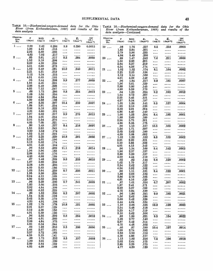
SUPPLEMENTAL DATA 43

TABLE 10.-Biochemical-oxygen-demand data for the Ohio TABLE 10.-Biochemical-oxygen-demand data for the Ohio River (from Kothandaraman, 1968) and results of the River (from Kothandaraman, 1968) and results of the data analysis data analysis-Continued

Observa- T BOD K1 Lo K1 var Observa- T BOD K1 Lo K1 var tion (K1l tion (K1) No. (days) (mg/1) (days-1) (mg/l) (days-1) (days-2 ) No. (days) (mg/1) (days-1 ) (mg/1) (days-1 ) (days-2 )

1 --- 0.99 2.42 0.286 9.8 0.280 0.0013 19 --- .98 1.76 .237 8.5 .218 .0003 1.86 4.19 .315 1.85 2.84 .201 2.95 5.60 .266 2.79 3.96 .235 4.85 7.02 .217 4.84 5.49 .200

2 --- .85 2.01 .317 8.5 .284 .0009 20 --- .89 1.47 .242 7.6 .211 .0006 1.52 3.18 .298 1.55 2.23 .201 2.60 4.39 .239 2.64 3.37 .219 4.51 6.06 .273 4.54 4.56 .174

3 --- 1.02 2.49 .281 10.0 .240 .0011 21 --- 1.02 1.32 .174 8.1 .164 .0002 2.21 4.21 .219 2.21 2.33 .136 3.12 5.24 .215 3.12 3.14 .166 4.91 6.63 .193 4.91 4.30 .149

4 --- .95 2.44 .298 9.9 .277 .0009 22 --- .96 1.84 .217 9.8 .181 .0007 1.96 4.35 .293 1.96 3.01 .159 2.88 5.40 .228 2.88 3.86 .145 4.83 7.12 .247 4.90 5.59 .170

5 --- .68 1.73 .286 9.8 .254 .0013 23 --- .64 1.23 .224 9.2 .193 .0012 1.68 3.55 .256 1.64 2.72 .207 2.59 4.84 .254 2.55 3.45 .131 4.89 6.58 .188 4.57 5.34 .197

6 --- .96 2.35 .267 10.4 .239 .0007 24 --- 1.01 1.26 .141 9.5 .127 .0004 1.88 3.91 .234 1.93 2.16 .126 2.86 5.18 .222 2.92 2.81 .094 4.81 6.80 .191 4.86 4.40 .140

7 --- 0.97 2.62 .317 9.9 .275 .0013 25 --- 1.00 1.55 .204 8.4 .195 .0001 1.84 4.01 .244 1.88 2.60 .189 2.93 5.54 .276 2.96 3.73 .201 4.85 7.05 .221 4.86 5.05 .175

8 --- .86 1.49 .227 8.4 .216 .0007 26 --- .90 1.13 .127 10.5 .105 .0002 1.53 2.53 .243 1.56 1.71 .097 2.59 3.52 .174 2.65 2.62 .100 4.52 5.18 .215 4.55 3.88 .092

9 --- 1.02 2.25 .229 10.8 .201 .0006 27 --- 1.02 1.22 .152 8.5 .135 .0002 2.21 4.03 .196 2.21 2.20 .121 3.12 5.02 .174 3.10 2.85 .122 4.91 6.49 .164 4.91 4.13 .142

10 --- .96 2.53 .269 11.1 .218 .0014 28 --- .96 1.34 .160 9.4 .142 .0003 1.96 3.96 .183 1.96 2.37 .137 2.88 5.03 .176 2.88 3.20 .137 4.83 6.98 .199 4.90 4.44 .110

11 --- .67 1.48 .268 9.0 .233 .0010 29 --- .62 .82 .144 9.6 .120. .0002 1.67 3.08 .239 1.62 1.79 .117 2.58 4.09 .206 2.54 2.62 .122 4.60 5.63 .186 4.56 3.92 .102

12 --- 1.03 2.04 .259 8.7 .226 .0011 30 --- .96 1.11 .131 9.4 .122 .0001 1.95 3.30 .228 1.88 2.06 .132 2.94 4.13 .169 2.86 2.78 .105 4.89 5.62 .202 4.81 4.16 .120

13 --- .96 2.29 .230 9.7 .241 .0009 31 --- .87 1.61 .316 6.7 .207 .0052 1.83 3.66 .235 1.87 2.41 .171 2.92 4.84 .199 2.92 3.07 .159 4.82 6.52 .223 4.75 3.84 .130

14 --- .88 1.52 .230 8.3 .207 .0005 32 --- .96 1.86 .241 9.0 .185 .0021 1.54 2.35 .198 1.56 2.62 .188 2.62 3.35 .170 2.60 3.42 .129 4.53 4.91 .198 4.44 4.64 .134

15 --- 1.02 1.79 .178 10.8 .151 .0005 33 --- 1.19 2.06 .155 12.2 .128 .0003 2.21 3.07 .129 2.54 3.48 .118 3.12 4.09 .156 3.23 4.17 .119 4.91 5.39 .120 5.10 5.62 .106

16 --- .96 2.35 .292 9.6 .254 .0018 34 --- .83 1.59 .221 9.5 .154 .0022 1.96 4.01 .260 1.98 2.77 .140 2.88 4.84 .175 2.87 3.42 .114 4.83 6.64 .244 4.75 4.48 .102

17 --- .66 1.23 .210 9.5 .186 .0006 35 --- .46 .87 .190 10.4 .157 .0014 1.66 2.67 .191 1.60 2.74 .192 2.57 3.72 .183 2.50 3.50 .116 4.59 5.15 .141 4.38 4.86 .117

18 --- .98 1.73 .232 8.5 .197 .0008 36 --- 1.13 1.82 .246 7.5 .196 .0018 1.90 2.81 .189 2.02 2.64 .175 2.89 3.64 .159 2.85 3.29 .173 4.83 4.99 .168 4.77 4.20 .129

44 MODEL FOR PREDICTING THE DISSOLVED-OXYGEN DEFICIT IN STREAMS

TABLE 10.-Biochemical-oxygen-demand data for the Ohio TABLE 10.-Bwchemical-oxygen-demand data for the Ohio River (from Kothandaraman, 1968) and results of the River (from Kothandaraman, 1968) and results of the data analysis-Continued data analysis-Continued ·

Observa- T BOD K1 Lo K1 var Observa- T BOD K1 Lo K1 var tion (days) (mg/1) (days-1) (mg/1) (days-1) (K1) tion (days) (mg/l) (days-1) (mg/1) (days-1) (K1) No. (days-2 ) No. (days-2 )

37 --- .87 1.61 .416 5.3 .286 .0095 55 --- .96 1.28 .201 7.3 .146 .0020 1.87 2.34 .220 1.56 1.60 .091 2.92 2.79 .157 2.60 2.16 .099 4.75 3.62 .219 4.44 3.46 .158

38 --- .96 1.68 .264 7.5 .208 .0019 56 --- 1.19 1.40 .130 9.8 .097 .0005 1.56 2.33 .197 2.54 2.22 .076 2.60 3.03 .140 3.23 2.66 .087 4.44 4.36 .192 5.10 3.62 .077

39 --- 1.19 1.70 .118 13.0 .090 .0005 57 --- .83 1.28 .207 8.1 .165 .0013 2.54 2.82 .077 1.98 2.46 .165 3.23 3.40 .085 2.87 3.21 .160 5.10 4.34 .055 4.75 4.08 .104

40 --- .83 1.44 .253 7.6 .174 .0037 58 --- .54 .59 .199 5.8 .152 .0018 1.98 2.46 .157 1.69 1.58 .183 2.87 3.13 .157 2.58 1.90 .089 4.75 3.76 .081 3.42 2.36 .149

41 --- .46 .82 .221 8.5 .163 .0026 59 --- 1.13 1.44 .164 8.5 .125 .0009 1.60 2.23 .178 2.02 2.16 .121 2.50 3.02 .150 2.85 2.66 .099 4.38 4.07 .113 4.77 3.54 .085

42 --- 1.13 1.79 .196 9.0 .168 .0014 60 --- .88 2.10 .119 21.1 .093 .0005 2.02 2.86 .180 1.88 3.42 .072 2.85 3.63 .161 2.75 4.72 .088 4.77 4.54 .097 4.88 6.75 .062

43 --- .87 1.57 .370 5.7 .274 .0044 61 --- .90 4.09 .186 26.6 .122 .0001 1.87 2.34 .206 1.81 6,19 .108 2.92 3.10 .244 2.40 7.20 .086 4.75 3.93 .210 4.52 10.43 .086

44 --- .96 1.39 .173 9.1 .119 .0012 62 --- 2.04 4.05 .101 21.8 .084 .0003 1.56 1.85 .103 3.23 5.43 .068 2.60 2.45 .083 5.00 6.95 .055 4.44 3.51 .094 6.96 9.07 .079

45 --- 1.19 1.74 .185 8.8 .154 .0007 63 --- 1.04 2.60 .199 13.9 .191 .0030 2.54 2.98 .143 1.79 4.61 .261 3.23 3.55 .149 2.98 5.88 .124 5.10 4.52 .109 4.75 7.60 .136

46 --- .82 1.34 .320 5.8 .260 .0166 64 --- .73 2.97 .244 18.2 .173 .0034 1.98 2.48 .254 1.35 4.88 .216 2.87 2.66 .063 2.54 6.72 .125 4.75 4.36 .415 4.31 8.71 .108

47 --- .54 .57 .144 7.6 .119 .0005 65 --- 1.04 3.42 .137 25.7 .121 .0005 1.69 1.54 .129 2.23 6.32 .117 2.58 1.96 .081 3.17 7.74 .081 3.42 2.48 .115 4.98 11.57 .133

48 --- 1.13 1.94 .226 8.6 .182 .0015 66 --- .94 1.54 .052 32.4 .048 .0001 2.02 2.89 .173 1.88 2.60 .037 2.85 3.62 .165 2.81 3.57 .036 4.77 4.63 .118 4.62 6.50 .059

49 --- .87 1.56 .315 6.5 .252 .0037 67 --- .88 1.50 .071 24.8 .051 .0002 1.87 2.68 .257 1.88 2.65 .051 2.92 3.50 .230 2.75 3.51 .046 4.75 4.20 .145 4.88 5.07 .036

50 --- .96 1.37 .234 6.8 .165 .0022 68 --- 2.04 6.03 .105 25.2 .116 .0004 1.56 1.74 .118 3.23 7.72 .078 2.60 2.34 .121 5.00 11.18 .125 4.44 3.36 .141 6.96 13.14 .077

51 --- .82 1.28 .164 10.2 .117 .0009 69 --- 1.01 2.30 .228 11.2 .204 .0006 1.98 2.40 .116 1.76 3.59 .209 2.87 3.00 .090 2.95 4.98 .169 4.75 4.11 .089 4.72 6.65 .177

52 --- .54 .60 .185 6.3 .130 .0021 70 --- .78 2.35 .180 17.9 .143 .0011 1.69 1.45 .140 1.35 3.67 .156 2.58 1.83 .092 2.54 5.82 .138 3.42 2.15 .088 4.31 7.61 .091

. 53 --- 1.13 1.73 .147 11.3 .107 .0009 71 --- 1.04 2.76 .094 29.7 .084 .0003 2.02 2.52 .097 2.23 5.22 .080 2.85 3.03 .072 3.17 6.42 .053 4.77 4.13 .106 4.98 10.23 .099

54 --- .87 1.58 .351 6.0 .313 .0336 72 --- .94 1.18 .051 25.4 .053 .0004 1.87 2.52 .239 1.88 2.26 .049 2.29 3.36 .658 2.81 3.22 .046 4.75 4.32 .184 4.62 5.44 .095

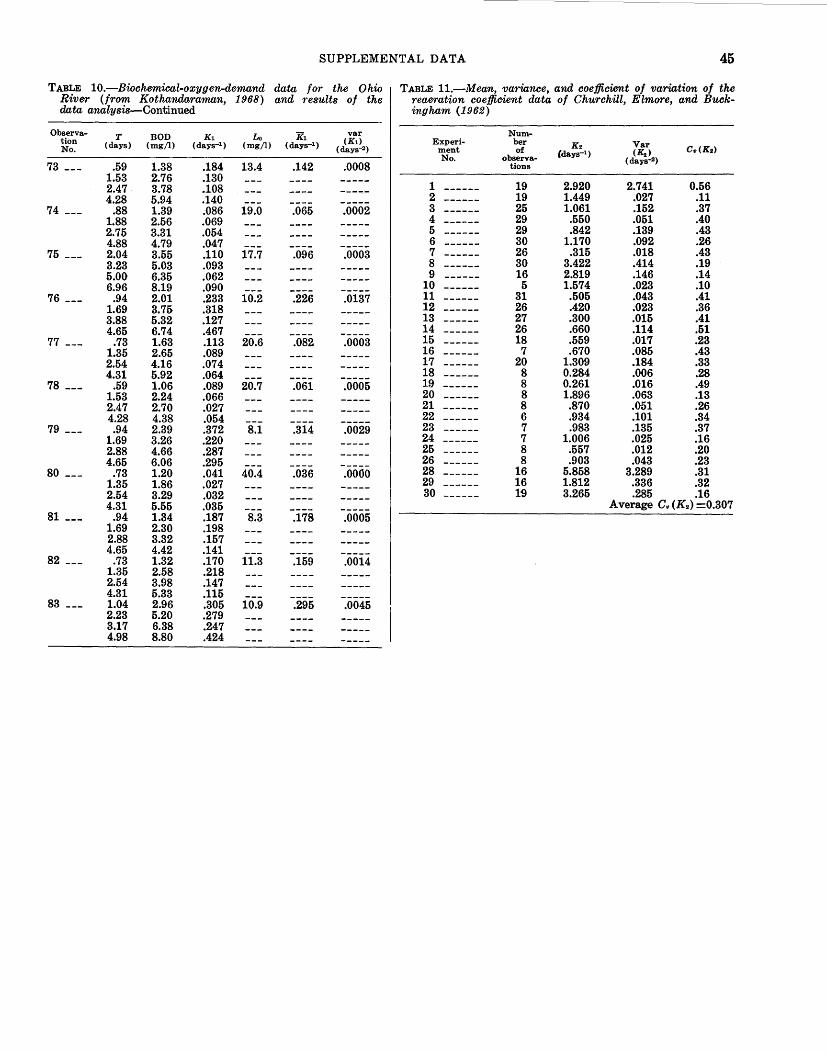
SUPPLEMENTAL DATA 45

TABLE 10.-Biockemical-oxygen-demand data for the Ohio TABLE ll.-Mean, variance, and coefficient of variation of the River (from Kothandaraman, 1968) and results of the reaeration coefficient data of Churchill, Elmore, and Buck-data analysis-Continued ingham (1962)

Observa- T BOD K1 Lo K1 var Num-tion (days) (mg/1) (days-1) (mg/1) (days-1) (K1) Experi- her K2 Var No. (days-2) ment of (days-1) (Kz) c.,(Kd

No. observa- (days-2) 73 --- .59 1.38 .184 13.4 .142 .0008 tions

1.53 2.76 .130 2.47 3.78 .108 1 19 2.920 2.741 0.56 4.28 5.94 .140 2 19 1.449 .027 .11

74 --- .88 1.39 .086 19.0 .065 .0002 3 25 1.061 .152 .37 1.88 2.56 .069 4 29 .550 .051 .40 2.75 3.31 .054 5 29 .842 .139 .43 4.88 4.79 .047 6 30 1.170 .092 .26

75 --- 2.04 3.55 .110 17.7 .096 .0003 7 26 .315 .018 .43 3.23 5.03 .093 8 30 3.422 .414 .19 5.00 6.35 .062 9 16 2.819 .146 .14 6.96 8.19 .090 10 5 1.574 .023 .10

76 --- .94 2.01 .233 10.2 .226 .0137 11 31 .505 .043 .41 1.69 3.71> .318 12 26 .420 .023 .36 3.88 5.32 .127 13 27 .300 .015 .41 4.65 6.74 .467 14 26 .660 .114 .51

77 --- .73 1.63 .113 20.6 .082 .0003 15 18 .559 .017 .23 1.35 2.65 .089 16 7 .670 .085 .43 2.54 4.16 .074 17 20 1.309 .184 .33 4.31 5.92 .064 18 8 0.284 .006 .28

78 --- .59 1.06 .089 20.7 .061 .0005 19 8 0.261 .016 .49 1.53 2.24 .066 20 8 1.896 .063 .13 2.47 2.70 .027 21 8 .870 .051 .26 4.28 4.38 .054 22 6 .934 .101 .34

79 --- .94 2.39 .372 8.1 .314 .0029 23 7 .983 .135 .37 1.69 3.26 .220 24 7 1.006 .025 .16 2.88 4.66 .287 21> 8 .557 .012 .20 4.65 6.06 .295 26 8 .903 .043 .23

80 --- .73 1.20 .041 40.4 .036 .0000 28 16 5.858 3.289 .31 1.35 1.86 .027 29 16 1.812 .336 .32 2.54 3.29 .032 30 19 3.265 .285 .16 4.31 5.55 .035 Average C., (K2) =0.307

81 --- .94 1.34 .187 8.3 .178 .0005 1.69 2.30 .198 2.88 3.32 .157 4.65 4.42 .141

82 --- .73 1.32 .170 11.3 .159 .0014 1.35 2.58 .218 2.54 3.98 .147 4.31 5.33 .115

83 --- 1.04 2.96 .305 10.9 .295 .0045 2.23 5.20 .279 3.17 6.38 .247 4.98 8.80 .424

46 MODEL FOR PREDICTING THE DISSOLVED-OXYGEN DEFICIT IN STREAMS

TABLE 12.-Correlation coefficient between the biochemical-oxygen-demand and the dissolved-oxygen concentration (from Moushegian and Krutchkoff, 1969)

Correlation coefficient, r(BOD, C)

K2 ----··------ 0.2 0.4 0.6 0.8 1.0 1.2 1.4 1.6 1.8 2.0 2.2 2.4 2.6

Kt T = 1 day

0.1 ---------- .70 .59 .52 .49 .46 .45 .43 .43 .42 .42 .41 .41 .41 .2 ---------- .69 .61 .56 .53 .51 .50 .48 .47 .46 .46 .45 .44 .3 ---------- .80 .70 .63 .59 .56 .53 .51 .50 .48 .47 .46 .45 .44 .4 ---------- .81 .64 .60 .56 .53 .51 .50 .48 .47 .46 .44 .43 .5 ---------- .81 .71 .64 .59 .56 .53 .51 .49 .47 .46 .44 .43 .42

Kt T = 2 days

0.1 ---------- .67 .56 .51 .48 .46 .45 .44 .43 .42 .41 .40 .39 .38 .2 ---------- .60 .53 .50 .47 .44 .43 .41 .39 .38 .36 .35 .34 .3 ---------- .70 .58 .52 .47 .44 .41 .39 .37 .36 .34 .32 .31 .30 .4 ---------- .68 .49 .41 .41 .38 .36 .34 .32 .30 .29 .27 .26 .5 ---------- .65 .53 .45 .41 .37 .34 .37 .30 .28 .27 .25 .24 .23

K1 T = 3 days

0.1 ---------- .63 .53 .48 .45 .43 .41 .39 .37 .35 .34 .32 .31 .29 .2 ---------- .52 .46 .41 .38 .36 .33 .31 .29 .28 .26 .25 .24 .3 ---------- .60 .47 .41 .36 .33 .30 .28 .26 .24 .23 .22 .24 .20 .4 ---------- .54 .35 .31 .27 .25 .23 .21 .20 .19 .17 .17 .16 .5 ---------- .49 .36 .30 .23 .21 .19 .19 .17 .16 .15 .14 .13 .13

Kt T = 4 days

0.1 ---------- .60 .50 .44 .41 .38 .35 .33 .31 .29 .27 .26 .25 .24 .2 ---------- .44 .38 .34 .30 .27 .25 .23 .22 .21 .20 .19 .18 .3 ---------- .49 .37 .31 .27 .24 .21 .19 .18 .17 .16 .15 .14 .13 .4 ---------- .41 .24 .21 .18 .16 .15 .13 .12 .12 .11 .10 .10 .5 ---------- .35 .24 .19 .16 .14 .12 .11 .10 .09 .09 .08 .08 .07

K1 T = 5 days

0.1 ---------- .56 .46 .40 .36 .32 .30 .27 .25 .24 .23 .21 .20 .20 .2 ---------- .37 .31 .27 .24 .21 .19 .18 .17 .16 .15 .14 .14 .3 ---------- .40 .29 .23 .19 .17 .15 .14 .12 .12 .11 .10 .10 .09 .4 ---------- .31 .17 .14 .12 .10 .09 .09 .08 .07 .07 .07 .06 .5 ---------- .24 .16 .12 .10 .08 .07 .06 .06 .05 .05 .05 .04 .04

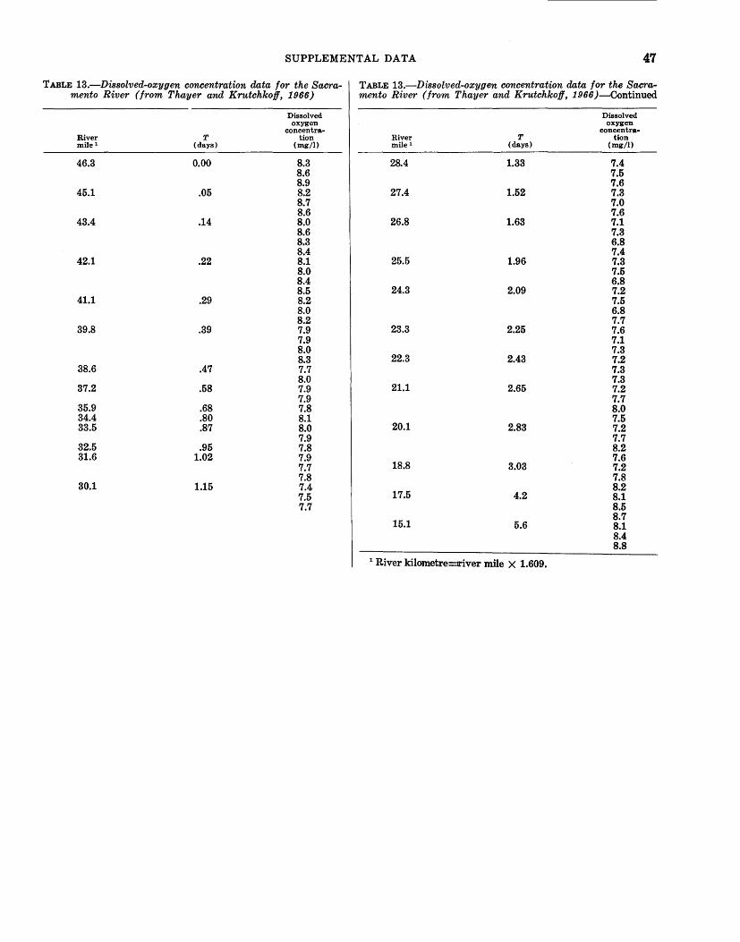
SUPPLEMENTAL DATA 47

TABLE 13.-Dissolved-oxygen concentration data for the Sacra- TABLE 13.-Dissolved-oxygen concentration data for the Sacra-mento River (from Thayer and Krutchkoff, 1966) mento River (from Thayer and Krutchkof!, 1966)-Continued

Dissolved Dissolved oxygen oxygen

con centra- con centra-River T tion River T tion mile 1 (days) (mg/1) mile 1 (days) (mg/l)

46.3 0.00 8.3 28.4 1.33 7.4 8.6 7.5 8.9 7.6

45.1 .05 8.2 27.4 1.52 7.3 8.7 7.0 8.6 7.6

43.4 .14 8.0 26.8 1.63 7.1 8.6 7.3 8.3 6.8 8.4 7.4

42.1 .22 8.1 25.5 1.96 7.3 8.0 7.5 8.4 6.8 8.5 24.3 2.09 7.2

41.1 .29 8.2 7.5 8.0 6.8 8.2 7.7

39.8 .39 7.9 23.3 2.25 7.6 7.9 7.1 8.0 7.3 8.3 22.3 2.43 7.2

38.6 .47 7.7 7.3 8.0 7.3

37.2 .58 7.9 21.1 2.65 7.2 7.9 7.7

35.9 .68 7.8 8.0 34.4 .80 8.1 7.5 33.5 .87 8.0 20.1 2.83 7.2

7.9 7.7 32.5 .95 7.8 8.2 31.6 1.02 7.9 7.6

7.7 18.8 3.03 7.2 7.8 7.8

30.1 1.15 7.4 8.2 7.5 17.5 4.2 8.1 7.7 8.5

15.1 8.7

5.6 8.1 8.4 8.8

1 River kilometre=river mile X 1.609.

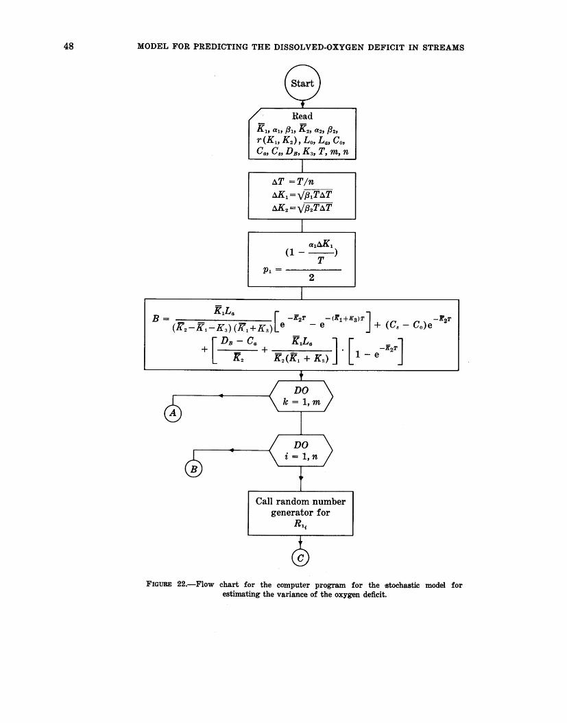
48 MODEL FOR PREDICTING THE DISSOLVED-OXYGEN DEFICIT IN STREAMS

KH ah {31, K2, a2, {32, r(Kh K2), Lo, La, Co, Ca, CB, DB, Ka, T, m, n

~T =Tin :---::==---:=

~K1 =yf31T~T

aK2 = v f32T ~T

P1 =-----2

Call random number generator for

R1i

FIGURE 22.-Flow chart for the computer program for the stochastic model for estimating the variance of the oxygen deficit.

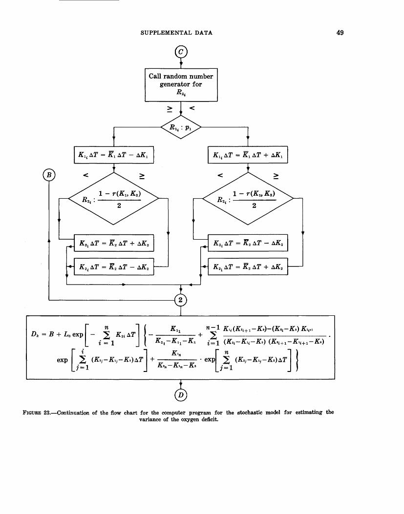
B

SUPPLEMENTAL DATA

Call random number generator for

R2,

FIGURE 23.-Continuation of the flow chart for the computer program for the stochastic model for estimating the variance of the oxygen deficit.

49

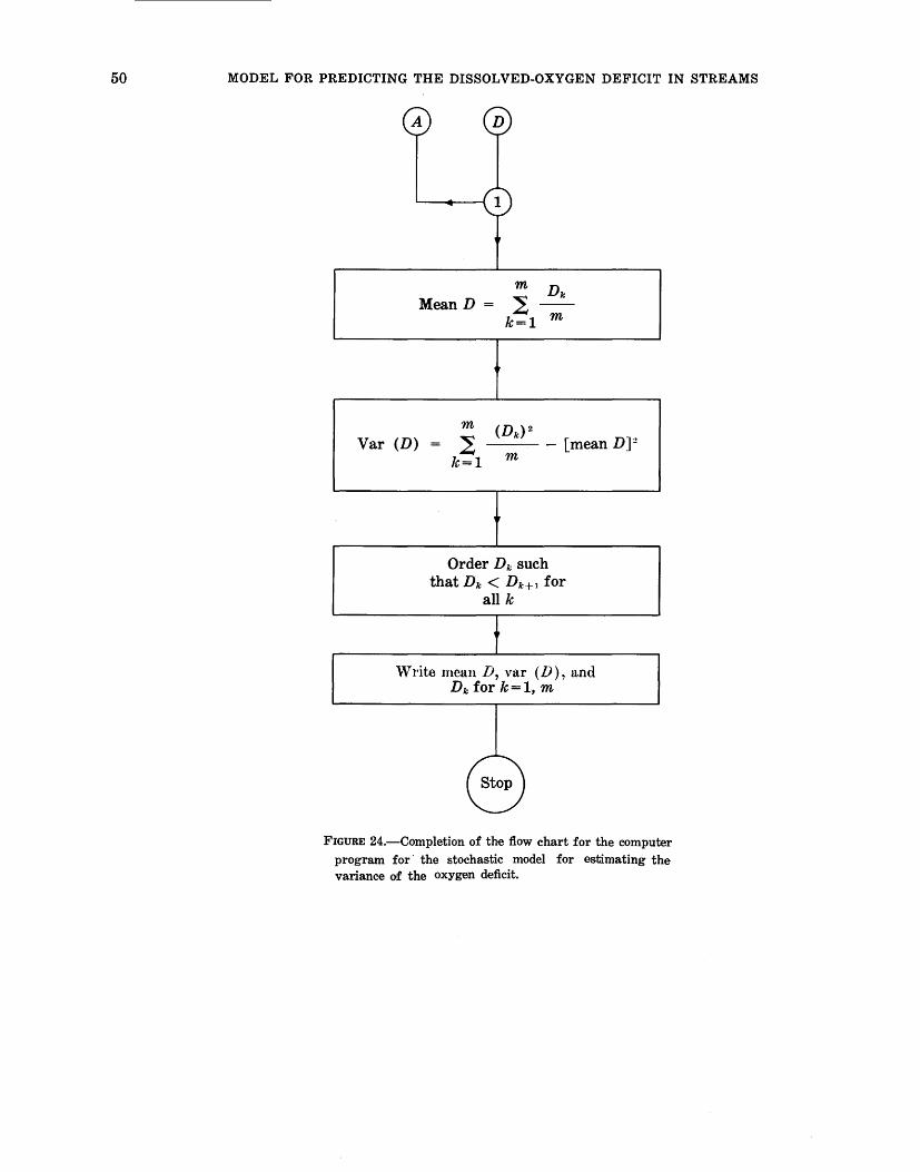
50 MODEL FOR PREDICTING THE DISSOLVED-OXYGEN DEFICIT IN STREAMS

A D

1

m Dk MeanD = ~ --

k=l m

m (Dk) 2

Var (D) = ~ -[mean DF k=l m

Order Dk such that Dk < Dk+1 for

all k

Write mean D, var (D), and Dk for k=l, m

Stop

FIGURE 24.-Completion of the flow chart for the computer program for· the stochastic model for estimating the variance of the oxygen deficit.