a stem-map model for predicting tree canopy …...a stem-map model for predicting tree canopy cover...

A Stem-map Model for Predicting Tree Canopy Cover of Forest Inventory and

Analysis (FIA) Plots

Chris Toney1, John D. Shaw2, and Mark D. Nelson3

Abstract: Tree canopy cover is an important stand characteristic that affects understory light, fuel moisture, decomposition rates, wind speed, and wildlife habitat. Canopy cover also is a component of most definitions of forest land used by US and international agencies. The USDA Forest Service Forest Inventory and Analysis (FIA) Program currently does not provide a national standard measurement of tree canopy cover, and most regional FIA units do not measure canopy cover in the field.

This paper describes a model for predicting canopy cover of FIA plots by mapping the locations of trees ≥ 5.0 in. diameter within the plot, and statistical modeling of sapling contribution to total cover. The model was developed with an operational focus, including the requirement that it scale efficiently to national applications. Coefficients for species-specific crown width equations have been stored in lookup tables with surrogates assigned to FIA tree species lacking equations. Modeling was supported by field measurements on 12,070 FIA plots distributed across the eight-state Interior West FIA region. Refinements to the model included adjustments to crown width equations for small-diameter trees, stem-mapping of microplot subsamples to support cover estimation of sapling-stage plots, and the use of spatial statistics to derive predictor variables describing the spatial pattern of overstory trees. Model predictions were compared to field measurements of canopy cover by line-intercept method on 1,454 single-condition plots from the Interior West FIA 2006 field season. The mean absolute difference between field-measured and model-predicted values was ± 7.9% canopy cover, with mean bias of -0.7% canopy cover. The relationship between field-measured and predicted values was approximately linear with approximately constant variance and a correlation coefficient r = 0.875.

FIA produces estimates of forest land area based on a definition of forest land that includes a minimum threshold of tree stocking. Proposed changes to the FIA definition from one based on stocking to one based on canopy cover could affect estimates of forest land area, but the amount and variability of this change is not fully understood. We made a preliminary assessment of the effect of a canopy cover-based definition on forest area estimates for a subset of states within the Northern Research Station FIA unit. Keywords: canopy cover, crown width, FIA, land cover, line intercept, Ripley’s K function, spatial pattern, stand height, stem-mapping 1 USDA Forest Service; Rocky Mountain Research Station; Inventory, Monitoring, and Analysis Program and the LANDFIRE Project; Missoula, MT 59808; email [email protected] 2 USDA Forest Service; Rocky Mountain Research Station; Inventory, Monitoring, and Analysis Program; Ogden, UT84401; email [email protected] 3 USDA Forest Service; Northern Research Station Forest Inventory and Analysis; St. Paul, MN 55108; email [email protected]

USDA Forest Service Proceedings – RMRS-P-56 53.

In: McWilliams, Will; Moisen, Gretchen; Czaplewski, Ray, comps. 2009. 2008 Forest Inventory and Analysis (FIA) Symposium; October 21-23, 2008: Park City, UT. Proc. RMRS-P-56CD. Fort Collins, CO: U.S. Department of Agriculture, Forest Service, Rocky Mountain Research Station. 1 CD.

Introduction

Canopy cover is defined as the proportion of the forest floor covered by a

vertical projection of the tree crowns (Jennings et al. 1999). Canopy cover influences the forest microclimate by affecting understory light, surface temperature, surface moisture levels, and wind speed (Jennings et al. 1999, Christopher and Goodburn 2008). It is a key stand characteristic used in a variety of applications (Shaw 2005). For example, canopy cover is often a component of wildlife habitat suitability models (Gill et al. 2000, Bond et al. 2004, Vospernik et al. 2007), and regional management plans for some species require maintaining certain levels of canopy cover (Fiala et al. 2006). In fire behavior simulation models such as FARSITE (Finney 2004), increasing canopy cover has a moderating effect on wind speed which is a driver of fire spread rate and partially determines situations where a ground fire is likely to transition to a crown fire. By shading the surface, canopy cover also determines dead fuel moisture levels under a given weather scenario. Canopy cover thresholds are a component of most international definitions of forest land, which has implications for reporting and carbon accounting (Lund 2002).

Plot-based data on canopy cover commonly are used to support these and other applications, but the Forest Inventory and Analysis (FIA) program of the USDA Forest Service currently does not have a national standard canopy cover measurement and most FIA regional units do not measure tree canopy cover in the field. However, FIA does use a national standard plot design and tree measurement protocol. An approach for modeling canopy cover, optimized for this plot design, could provide canopy cover data that are estimated consistently across the nation. Our objective was to develop a model for predicting tree canopy cover of FIA plots along with software for efficient data processing.

FIA currently produces estimates of forest land area based on a definition of forest land that includes a minimum threshold of tree stocking. Land that formerly was stocked (e.g., clear-cuts) is still considered forest if not developed for other uses (Bechtold and Patterson 2005: glossary, page 80). A proposed change to the FIA definition of forest land could replace the minimum stocking threshold with a threshold of minimum canopy cover, but presumably would retain some form of the land-use requirement in the definition. This change could affect estimates of forest land area, but the amount, direction, and spatial variability of this potential effect are not fully understood. A second objective was to make a preliminary assessment of the effect of a canopy cover-based definition on forest area estimates for a subset of states within the Northern Research Station (NRS) FIA unit.

2


Methods Canopy Cover Data and Modeling Approach Additional background on the data and modeling approach was presented by Shaw (2005). The current FIA standard plot design was described in detail by Bechtold and Scott (2005) and is summarized in figure 1.

2Subplot:

Figure 1: FIA national standard plot layout. Microplot centers are 12 ft. at 90º azimuth from subplot centers. The minimum circle enclosing all four subplots is approximately 1.5 ac. Not shown are optional 58.9-ft. radius macroplots surrounding each subplot.

Details of the tree measurements are described in the FIA field manual (USDA Forest Service 2005). Diameters are generally measured at breast height (DBH), but for some western woodland species (USDA Forest Service 2007) diameters are measured at the root collar (DRC). DBH is measured to the nearest tenth of an inch at a point 4.5 feet above ground level on the uphill side of the tree. DRC is measured to the nearest tenth inch at the ground line or at the stem root collar, whichever is higher. Reference herein to stem diameter means DBH or DRC.

A key feature of the tree measurement protocol is that a coordinate is recorded for each tree ≥ 5.0 in. diameter in the subplots, and for each tree ≥ 1.0 in. diameter but < 5.0 in. diameter in the microplots. Trees ≥ 1.0 in. diameter but < 5.0 in. diameter are denoted as saplings by FIA, and are measured in the microplots. Coordinates are recorded as distance and azimuth from the microplot centers for saplings, and from subplot centers for trees ≥ 5.0-in. diameter.

24.0 ft. radius

1

34

120 ft. between subplot centers

Microplot: 6.8 ft. radius

3


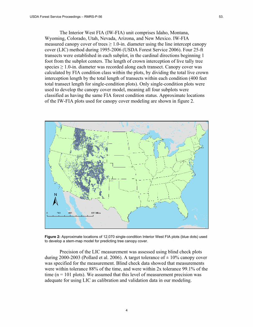
The Interior West FIA (IW-FIA) unit comprises Idaho, Montana, Wyoming, Colorado, Utah, Nevada, Arizona, and New Mexico. IW-FIA measured canopy cover of trees ≥ 1.0-in. diameter using the line intercept canopy cover (LIC) method during 1995-2006 (USDA Forest Service 2006). Four 25-ft transects were established in each subplot, in the cardinal directions beginning 1 foot from the subplot centers. The length of crown interception of live tally tree species ≥ 1.0-in. diameter was recorded along each transect. Canopy cover was calculated by FIA condition class within the plots, by dividing the total live crown interception length by the total length of transects within each condition (400 feet total transect length for single-condition plots). Only single-condition plots were used to develop the canopy cover model, meaning all four subplots were classified as having the same FIA forest condition status. Approximate locations of the IW-FIA plots used for canopy cover modeling are shown in figure 2.

Figure 2: Approximate locations of 12,070 single-condition Interior West FIA plots (blue dots) used to develop a stem-map model for predicting tree canopy cover. Precision of the LIC measurement was assessed using blind check plots during 2000-2003 (Pollard et al. 2006). A target tolerance of ± 10% canopy cover was specified for the measurement. Blind check data showed that measurements were within tolerance 88% of the time, and were within 2x tolerance 99.1% of the time (n = 101 plots). We assumed that this level of measurement precision was adequate for using LIC as calibration and validation data in our modeling.

4


Bechtold (2003, 2004) developed regression equations that predict tree crown width from stem diameter and other predictor variables for 140 tree species in the United States. We used the equations from Bechtold (2003, 2004) that predict crown width from stem diameter. Surrogates were assigned to species lacking an equation based on similarities in tree crown shape. Since the model-fitting data used by Bechtold (2003, 2004) did not include trees < 5.0 in. diameter, we estimated crown width adjustment factors for saplings based on data from Bragg (2001). The crowns of trees ≥ 5.0-in. diameter were modeled as symmetrical, circular polygons with area estimates based on the species-specific crown width equations. The modeled tree crowns were mapped within each subplot by placing the center of each crown at the coordinates recorded by field crews for stem-locations (figure 3). Canopy cover of trees ≥ 5.0-in. diameter was estimated by computing the proportion of the subplot polygons intersected by the mapped tree crowns, and then averaging the four subplot values to get a plot-level estimate (hereafter, referred to as SMCsubp, i.e., stem-map canopy cover of trees ≥ 5.0-in. diameter in the subplots). Canopy cover, by definition, was constrained to the 0 to100% range. The procedure was repeated for saplings in the microplots to compute a separate estimate of sapling canopy cover at the plot level, not accounting for overlap by the larger trees (SMCmicr). Geometric computations were done with a custom C program using the Geometry Engine Open Source library (http://trac.osgeo.org/geos/).

Figure 3: Example of mapping modeled crowns of trees ≥ 5.0-in. diameter in an FIA plot based on stem coordinates recorded by field crews. Measured stem diameters are drawn to scale as brown circles in the expanded view of subplot 1.

Because only trees ≥ 5.0-in. diameter can be stem-mapped across the entire FIA subplot cluster, we expected that SMCsubp would under-estimate LIC on average since LIC included all trees ≥ 1.0-in. diameter, including those < 5.0-in. To provide model-estimated canopy cover of trees ≥ 1.0-in. diameter, we developed a linear regression equation to predict the contribution of saplings to

5


total canopy cover. SMCsubp was compared to LIC, and a residual was calculated for each plot as e = LIC - SMCsubp. We assumed that e was due primarily to the exclusion of saplings from SMCsubp, and we expected e would be correlated with SMCmicr. However, since saplings may be overtopped by larger trees, a portion of the sapling cover may not contribute to total canopy cover in a given plot. The contribution of saplings to total canopy cover could also depend on other stand characteristics such as the density, height, and spatial pattern of larger trees. Estimates of Ripley’s K function (Ripley 1991, Venables and Ripley 2002) were used to account for the spatial pattern of trees ≥ 5.0-in. diameter. Ripley’s K is useful for summarizing certain aspects of a pattern of points within a defined observation window, in this case, tree stem locations within the four subplots of an FIA plot. It can suggest whether an observed point pattern is either more clustered or more regularly spaced than would be expected for a random arrangement of the points. K(r) is a function of a distance r around each point in the pattern. The spatstat package version 1.11-7 (Baddeley and Turner 2005) for R (R Development Core Team 2006) was used to estimate K(r) for distances of 6, 8, 10, and 12 feet. The Kest function in spatstat estimates K(r) from a homogenous point pattern in a window of arbitrary shape. We specified the border method (Ripley 1991) in spatstat for edge correction of the point-pattern calculations. For regression modeling we worked with the square-root transformation L(r) = π/)(rK , which stabilizes variance (Stoyan and Penttinen 2000). Potential predictor variables considered for a regression model to predict e were:

SMCmicr = stem-mapped canopy cover estimate of saplings in the microplots numSaplings = total number of saplings measured in the microplots numTrees = total number of live trees ≥ 5.0 in. diameter measured in the subplots meanTreeHtBAW = basal area-weighted mean height (ft.) of trees ≥ 5.0 in. diameter meanL = mean of L(6 ft), L(8 ft), L(10 ft), and L(12 ft)

Single-condition IW-FIA plots measured during 1995 through 2005 were used for model fitting, and the 2006 plots were withheld as a validation set. Crown width models for certain western oak species (e.g., Gambel oak Quercus gambelii) had relatively large prediction errors (Bechtold 2004) and a review of plot photos in oak woodland forest types suggested that LIC would have relatively large measurement errors in these forest types. Plots classified as oak woodland forest types (FIA forest type codes 925 and 926) were removed from the model fitting data so they would not influence regression estimates. No plots were removed from the validation set. Linear regression models were fit using the lm function in R 2.4.1 (R Development Core Team 2006).

6


Smooth curves fitted by local polynomial regression (Venables and Ripley 2002) were used in exploratory analysis and as an aid to the interpretation of scatterplots in the Results. Smooth regression curves were fit with the loess.smooth function in R using the default span parameter of 2/3 (R Development Core Team 2006). Assessment of Forest Area Estimates in NRS

Four of the 24 states within the NRS-FIA were selected to represent a range of conditions across the region, e.g., a range in latitude and longitude, temperature, precipitation, and dominant forest types. Selected states included: Michigan (MI), Missouri (MO), Pennsylvania (PA), and South Dakota (SD). Only plots from annual inventory years 2002 to 2006 were included, which was the most current evaluation group as of 5 August 2008. Compared with a base federal sampling intensity of one plot per approximately 6,000 acres, sampling intensity during this period was tripled in MI, doubled in southern MO, and at single (base) intensity in PA and SD. Nearly 375,000 tree records were queried from 10,075 plots where all conditions were forest land (i.e., 100 percent forested plots) and plots had tree records. Per-state estimates of forest land area and accompanying sampling errors were produced using FIA’s EVALIDator web-based estimation tool (http://www.fia.fs.fed.us/tools-data/other/). Estimates were produced for 1) all forest land with stocking of at least 10 percent, including seedlings, 2) all forest land with stocking of at least 10 percent, excluding seedlings, and 3) all forest land with model-estimated canopy cover of at least 10 percent (excludes seedlings). For comparison, estimates also were produced for 1) all forest land area, including all plots of any stocking, regardless of tree presence or condition proportion (equivalent to FIA’s reported estimates of forest land area), and 2) forest land area of any stocking, but based on the queried subset of plots having tree records and 100 percent forested conditions. The last two estimates were used to determine 1) the reduction in estimated forest area resulting from constraining plots to a minimum of 10 percent stocking or canopy cover, and 2) the reduction in estimated forest area resulting from constraining plots to those with trees and 100 percent forested conditions.

Results Canopy Cover Model

As expected, SMCsubp tended to underestimate LIC (figure 4). The mean difference (LIC - SMCsubp) was 9.0% canopy cover, while the mean absolute difference (|LIC - SMCsubp|) was ±11.6% canopy cover (n = 12,070 plots).

7


1:1

stem-map canopy cover of trees ≥ 5.0 in. diameter (%)

line

inte

rcep

t can

opy

cove

r of

tree

s ≥

1.0

in. d

iam

eter

(%)

Figure 4: Comparison of the field-measured line intercept canopy cover of trees ≥ 1.0 in. diameter versus canopy cover of trees ≥ 5.0 in. diameter estimated by stem-mapping (n = 12,070 plots).

The data set shown in figure 4 was split into two subsets to examine the effect of sapling presence on the mean difference between stem-map and line-intercept canopy cover. Figure 5a shows the comparison of SMCsubp versus LIC for the subset of plots that had at least one sapling recorded in the microplots. SMCsubp underestimated LIC by an average of 11.4% canopy cover for these plots, while the mean absolute difference was ±13.7% canopy cover (n = 7,794 plots). Figure 5b shows the comparison of SMCsubp versus LIC for the subset of plots that had no saplings detected by the microplot subsample. SMCsubp underestimated LIC by an average of 4.7% canopy cover for these plots, while the mean absolute difference was ±7.7% canopy cover (n = 4,276 plots). The plots shown in figure 5a had low to high sapling canopy cover, while the plots shown in figure 5b likely had zero to low sapling canopy cover since the microplots are a 1/12th subsample of each subplot. Some of the remaining 4.7% mean difference between SMCsubp and LIC is likely due to sapling cover not detected by the microplot sample.

8


1:1


line

inte

rcep

t can

opy

cove

r of

tree

s ≥

1.0

in. d

iam

eter

(%)

(a)

1:1


line

inte

rcep

t can

opy

cove

r of

tree

s ≥

1.0

in. d

iam

eter

(%)

(b)

Figure 5: (a) Comparison of the field-measured line intercept canopy cover of trees ≥ 1.0 in. diameter versus canopy cover of trees ≥ 5.0 in. diameter estimated by stem-mapping, for the subset of plots that had at least one sapling recorded in the microplots (n = 7,794 plots), and (b) comparison of the field-measured line intercept canopy cover of trees ≥ 1.0 in. diameter versus canopy cover of trees ≥ 5.0 in. diameter estimated by stem-mapping, for the subset of plots that had no saplings detected by the microplot sample (n = 4,276 plots).

9


Residual canopy cover from the comparison of SMCsubp to LIC was positively correlated with SMCmicr (figure 6). In plots having low (<10%) canopy cover of trees ≥ 5.0 in. diameter, we assumed that overtopping of saplings by the crowns of larger trees was negligible, and total canopy cover was estimated by SMCsubp + SMCmicr. In plots having SMCsubp ≥ 10%, we assumed that saplings could be overtopped to some extent by the larger trees. For these plots, we estimated the sapling component of total canopy cover by multiple linear regression, taking into account the vertical structure and spatial pattern of the larger trees in addition to SMCmicr. The residual canopy cover (e = LIC - SMCsubp) shown in figure 6 was the dependent variable. Summary statistics for the variables used in regression analysis are shown in table 1, and estimated regression coefficients for predicting e are in table 2.

loess

stem-map canopy cover of saplings (%)

resi

dual

s

r = 0.38p < 0.001

Figure 6: Relationship between canopy cover of saplings estimated by stem-mapping the microplots, and residuals calculated as the field-measured line intercept canopy cover of trees ≥ 1.0 in. diameter minus the canopy cover of trees ≥ 5.0 in. diameter estimated by stem-mapping the subplots. The orange line is a smooth regression curve fitted with the loess.smooth function in R.

Table 1: Ranges, means, and standard deviations of the variables used in a linear regression model to estimate the sapling component of total canopy cover. Residual canopy cover (e = LIC - SMCsubp) was the dependent variable. Variable Minimum Mean Std. dev. Maximum residual canopy cover (%) -39 10.0 13.2 73 SMCmicr (%) 0 10.1 11.9 89 numSaplings 0 3.6 5.2 60 numTrees 1 27.3 17.2 132 meanTreeHtBAW (ft) 4.2 42.3 25.0 137.9 meanL 0 9.4 3.9 35.3

10


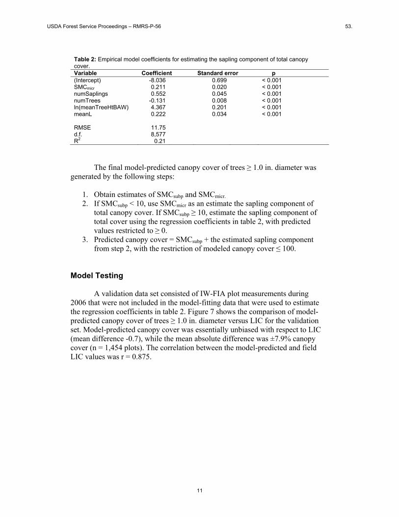
Table 2: Empirical model coefficients for estimating the sapling component of total canopy cover. Variable Coefficient Standard error p (Intercept) -8.036 0.699 < 0.001 SMCmicr 0.211 0.020 < 0.001 numSaplings 0.552 0.045 < 0.001 numTrees -0.131 0.008 < 0.001 ln(meanTreeHtBAW) 4.367 0.201 < 0.001 meanL 0.222 0.034 < 0.001 RMSE 11.75 d.f. 8,577 R2 0.21

The final model-predicted canopy cover of trees ≥ 1.0 in. diameter was generated by the following steps:

1. Obtain estimates of SMCsubp and SMCmicr. 2. If SMCsubp < 10, use SMCmicr as an estimate the sapling component of

total canopy cover. If SMCsubp ≥ 10, estimate the sapling component of total cover using the regression coefficients in table 2, with predicted values restricted to ≥ 0.

3. Predicted canopy cover = SMCsubp + the estimated sapling component from step 2, with the restriction of modeled canopy cover ≤ 100.

Model Testing

A validation data set consisted of IW-FIA plot measurements during 2006 that were not included in the model-fitting data that were used to estimate the regression coefficients in table 2. Figure 7 shows the comparison of model-predicted canopy cover of trees ≥ 1.0 in. diameter versus LIC for the validation set. Model-predicted canopy cover was essentially unbiased with respect to LIC (mean difference -0.7), while the mean absolute difference was ±7.9% canopy cover (n = 1,454 plots). The correlation between the model-predicted and field LIC values was r = 0.875.

11


1:1

modeled canopy cover of trees ≥ 1.0 in. diameter (%)

line

inte

rcep

t can

opy

cove

r of

tree

s ≥

1.0

in. d

iam

eter

(%)

loess

Figure 7: Comparison of field-measured line intercept canopy cover of trees ≥ 1.0 in. diameter versus model-predicted canopy cover of trees ≥ 1.0 in. diameter for the validation plots measured in 2006 (n = 1,454 plots).The orange line is a smooth regression curve fit to the data points with the loess.smooth function in R.

Forest Area Estimates

Estimates of all forest land area were 19,544,600 acres in MI, 15,078,279 acres in MO, 16,599,569 acres in PA, and 1,734,724 acres in SD (figure 8). Estimates of forest land area decreased when constrained to minimum thresholds of 1) at least 10 percent stocking of trees and seedlings (0.5 – 7.4 percent decrease), 2) at least 10 percent stocking of trees ≥ 1 in. DBH (0.4 – 9.6 percent decrease), or 3) at least 10 percent model-estimated canopy cover of trees ≥ 1 in. DBH (0.3 – 8.0 percent decrease). This equated to excluding nonstocked forest land from FIA estimates, and also excluding seedlings from the latter two criteria. South Dakota, the state with the lowest mean stocking and canopy cover, showed the largest percent decreases. However, none of differences among forest land area estimates based on the varying criteria for stocking and canopy cover within each state were statistically significant. Decreases due to excluding nonstocked plots and seedlings from the minimum canopy cover-based estimates were nearly identical to decreases due to excluding nonstocked plots and seedlings from the minimum stocking-based estimates.

12


Forest land area

0

5 000 000

10 000 000

15 000 000

20 000 000

Michigan Missouri Pennsylvania South Dakota

Acr

es

Forest Land

ALSTK >= 10%

LT1STK >= 10%

MODEL_CRCOV >= 10%

Figure 8: Forest land area estimates for selected states in NRS-FIA based on different criteria for stocking and canopy cover. Forest land = current FIA estimates of forest land area that include a land-use component in the definition of forest land. ALSTK = estimates based only on a minimum threshold for all tree stocking (trees, saplings, seedlings). LT1STK = estimates based only on a minimum threshold for stocking of trees ≥ 1 in. DBH (excludes seedlings). MODEL_CRCOV = estimates based only on a minimum threshold for model-estimated canopy cover of trees ≥ 1 in. DBH (excludes seedlings). Bars indicate 95% confidence intervals.

Discussion The canopy cover model described here makes use of the tree spatial information available for FIA plots. Aspatial methods for estimating plot-level canopy cover may assume a random tree distribution (e.g., Crookston and Stage 1999). Compared with aspatial methods, a model based on stem-mapping could avoid bias when tree distributions are nonrandom, especially in stands with regular tree spacing such as plantations (Christopher and Goodburn 2008). Explicitly incorporating tree spatial pattern into the model is also expected to improve precision of the estimates compared with an aspatial approach. Some characteristics of modeled canopy cover may be beneficial for certain applications. Model-estimated canopy cover is fully defined with respect to species and individual tree variables, e.g., “canopy cover of species considered tree life form by FIA (USDA Forest Service 2007) and having minimum stem diameter of 1 in.” In contrast, estimates of plot-level canopy cover derived from aerial photos generally are limited in terms of species and size class

13


discrimination, and may confuse tree canopy with background vegetation and shadows. Modeling canopy cover from tree data provides the flexibility of estimating various components of the total cover, such as canopy cover by species or canopy cover within different height layers. Field measurement of various canopy cover components, in addition to total tree cover, may be too costly to implement in some inventories since the time required on each plot would increase. A canopy cover model optimized for FIA plots provides a large data set at low additional cost, with prediction errors that may be tolerable in several applications.

FIA’s current definition of forest land includes both a land-cover and a land-use component, and also implies potential future stocking. Although a minimum threshold of 10% stocking is specified, land that formerly was stocked (e.g., clear-cuts) is still considered forest if not developed for other uses (Bechtold and Patterson 2005). A proposed shift from a stocking- to a cover-based definition of forest land could retain a land-use requirement and likely would imply a minimum potential future canopy cover. Our analysis suggests that differences in forest area estimates resulting from the proposed change to a cover-based definition could be negligible. These results should be considered as preliminary since they included only four selected states in the NRS-FIA region, and model-estimated canopy cover was subject to the caveats described below. Caveats and Current Limitations

The canopy cover model described above contains two parts: a geometric model of tree crowns within FIA subplots and an empirical model of the sapling contribution to total canopy cover that accounts for potential overlap from the crowns of larger trees. The empirical model was based on line-intercept field data collected within the IW-FIA region. Performance of the empirical model when extrapolated to other regions is currently unknown. It would be desirable for FIA to measure line-intercept canopy cover on at least a subset of plots in all regions. A 1/16th subset like the FIA Phase 3 sample (Reams et al. 2005) should provide sufficient data for regional validation and calibration of canopy cover models, while adding only slightly to the time it takes to complete the plot measurements. Canopy cover estimates based on mapping modeled tree crowns within the subplots currently do not include edge correction (not to be confused with edge correction applied to estimates of Ripley’s K which deal strictly with point patterns derived from the stem coordinates). A possible source of bias is the presence of trees with stems outside the subplot boundary, but having crowns that cover a portion of the subplot. Since the line-intercept reference data used in the present study included trees ≥ 1.0 in. diameter, bias due to edge effects is confounded with bias due to omitting the saplings from the subplot stem-maps. Our analysis suggests that the remaining bias due to edge effects is probably small once saplings have been accounted for (cf. Nelson et al. 1997). However,

14


incorporating an edge correction method (e.g., Williams et al. 2003) would be desirable in a future version of the model. Model development has focused so far on canopy cover estimation at the whole-plot level for single-condition plots. The model is expected to extend to multi-condition plots in which all condition classes are forested and could be used to estimate canopy cover of the whole plot footprint when a portion of the plot is nonforest. The model currently does not estimate canopy cover by condition, and multi-condition plots have not been used in model development or testing. The BOUNDARY table in FIADB (USDA Forest Service 2007) could be used to construct irregular subplot polygons when multiple conditions have been mapped within a subplot. This could support canopy cover estimation by condition, but the edge effects discussed above would become more problematic in small polygons. Future development of the model should address multi-condition plots. Seedlings were not included in the IW-FIA line intercept measurements of canopy cover taken during 1995-2006, and we did not attempt to incorporate the seedling component of total cover into the model. However, in 2007 IW-FIA began including seedlings in the line-intercept measurements. It is possible that sufficient data are now available to account for seedlings in model-estimated canopy cover. The national standard seedling count from the microplots is a potential predictor variable. Future model development could address the seedling component of total cover. The stem-map model also could be extended to produce canopy cover estimates by individual tree species as well as estimates within specified height layers. This functionality could be useful in applications such as wildlife habitat analysis and vegetation classification. Software for Data Processing Production of plot-level canopy cover estimates has been automated, requiring only a subset of the FIADB TREE table (USDA Forest Service 2007) as input (figure 9). The software avoids the use of a GIS for performance considerations and is based on open-source libraries. Crown widths are calculated using coefficients stored in lookup tables that have been populated for FIA tree species nationally based on Bechtold (2003, 2004). The software and lookup tables currently accommodate crown width equations of the quadratic form fit by Bechtold (2003, 2004) as well as a three-parameter nonlinear power function (Bragg 2001) and nonlinear power function in logarithmic scale (Shaw 2005). Users can mix these equation types if needed and substitute localized equations if available. Stem-map output variables are listed in table 3.

15


subset ofFIADB TREE

table

crown widthcoefficient

table

stemMapCanopy.py

GEOS C API

spatstatvia RPy

stem-mapoutputs

Figure 9: Flow chart describing a data processing system that implements the stem-map canopy cover model version 1.6. Lookup tables containing coefficients for crown width equations are populated for FIA tree species nationally. Batch processing is done with a Python program. Overlay of tree crowns on subplots and microplots is implemented in a C function using the Geometry Engine Open Source (GEOS) library. Estimates of Ripley’s K are obtained from the Kest function in the spatstat package for R, called from Python via the RPy interface. The tabular output includes plot ids along with canopy cover estimates at the whole plot and subplot levels, several stand height metrics, and tree spatial pattern statistics.

Table 3: Outputs from FIA stem-map model version 1.6. Variable Description map_crcov_subp Estimated canopy cover of trees ≥ 5-in. diameter from crown-

mapping the subplots (average of four subplots) map_crcov_subp_sn Estimated canopy cover of trees ≥ 5-in. diameter in subplot n from

crown-mapping (n = 1 – 4) map_crcov_micr Estimated canopy cover of saplings from crown-mapping the

microplots (average of four microplots) map_crcov_micr_sn Estimated canopy cover of saplings in the microplot of subplot n

from crown-mapping (n = 1 – 4) model_crcov Estimated total canopy cover of trees ≥ 1-in. diameter, derived from

crown-mapped subplots plus a regression estimate of the sapling component

meanTreeHt Mean height of trees ≥ 5.0 in. diameter meanTreeHtBAW Basal-area weighted mean height of trees ≥ 5.0 in. diameter meanTreeHtDom Mean height of canopy dominant/co-dominant trees ≥ 5.0 in.

diameter meanTreeHtDomBAW Basal-area weighted mean height of canopy dominant/co-dominant

trees ≥ 5.0 in. diameter maxTreeHt Height of the tallest tree ≥ 5.0 in. diameter predomTreeHt Predominant tree height (mean height of the tallest trees ≥ 5.0 in.

diameter comprising 16 trees per acre) meanSapHt Mean height of saplings (≥ 1.0 in. diameter and < 5.0 in. diameter) maxSapHt Height of the tallest sapling K_rft Estimates of Ripley’s K function at r feet (r = 6, 8, 10, and 12) L_rft Estimates of Ripley’s L function at r feet (r = 6, 8, 10, and 12) G_rft Estimates of the nearest neighbor distribution function at r feet (r = 6,

8, 10, and 12)

16


Acknowledgements Many thanks go to the data collection and compilation staff of the USDA Forest Service FIA Program who made this work possible. Portions of this work were performed under a Memorandum of Understanding between FIA and the inter-agency LANDFIRE Project (www.landfire.gov) in support of vegetation mapping in LANDFIRE. Sara Goeking and Will McWilliams provided helpful comments on the paper.

Literature Cited Baddeley, A. and R. Turner. 2005. Spatstat: an R package for analyzing spatial point

patterns. J. Stat. Software 12:(6)1-42. Bechtold, W.A. 2003. Crown-diameter prediction models for 87 species of stand-grown

trees in the eastern United States. South. J. Appl. For. 27(4):269-278. Bechtold, W.A. 2004. Largest-crown-width prediction models for 53 species in the

western United States. West. J. Appl. For. 19(4):245-251. Bechtold, W.A., and P.L. Patterson (eds.). 2005. The enhanced Forest Inventory and

Analysis program – national sampling design and estimation procedures. USDA For. Serv. Gen. Tech. Rep. SRS-80.

Bechtold, W.A. and C.T. Scott. 2005. The forest inventory and analysis plot design. P.

27-42 in The enhanced Forest Inventory and Analysis program – national sampling design and estimation procedures, Bechtold, W.A., and P.L. Patterson (eds.) USDA For. Serv. Gen. Tech. Rep. SRS-80.

Bond, M.L, M.E. Seamans, and R.J. Gutiérrez. 2004. Modeling nesting habitat selection

of California spotted owls (Strix occidentalis occidentalis) in the central Sierra Nevada using standard forest inventory metrics. For. Sci. 50(6):773-780.

Bragg, D.C. 2001. A local basal area adjustment for crown width prediction. North. J.

Appl. For. 18(1):22-28. Christopher, T.A. and J.M. Goodburn. 2008. The effects of spatial patterns on the

accuracy of Forest Vegetation Simulator (FVS) estimates of forest canopy cover. West. J. Appl. For. 23(1):5-11.

Crookston, N.L. and A. R. Stage. 1999. Percent canopy cover and stand structure

statistics from the Forest Vegetation Simulator. USDA For. Serv. Gen. Tech. Rep. RMRS-GTR-24. 11 p.

Fiala, A.C.S, S.L. Garman, and A.N. Gray. 2006. Comparison of five canopy cover

estimation techniques in the western Oregon Cascades. For. Ecol. Manage. 232:188-197.

17


Finney, M.A. 2004. FARSITE: Fire Area Simulator-model development and evaluation. Res. Pap. RMRS-RP-4, USDA For. Serv., Ogden, Utah. 47 p.

Gill, S.J., G.S. Biging, and E.C. Murphy. 2000. Modeling conifer tree crown radius and

estimating canopy cover. For. Ecol. Manage. 126:405-416. Jennings, S.B., N.B. Brown, and D. Sheil. 1999. Assessing forest canopies and

understorey illumination: canopy closure, canopy cover and other methods. Forestry 72(1):59-73.

Lund, H.G. 2002 When is a forest not a forest? J. Forestry 100(8):21-28. Nelson, R.F., T.G. Gregoire, and R.G. Oderwald. 1997. The effects of fixed-area plot

width on forest canopy height simulation. For. Sci. 44(3):438-444. Pollard, J.E., J.A. Westfall, P.L. Patterson, D.L. Gartner, M. Hansen, and O. Kuegler.

2006. Forest Inventory and Analysis national data quality assessment report for 2000 to 2003. USDA For. Serv. Gen. Tech. Rep. RMRS-GTR-181. 43p.

R Development Core Team. 2006. R: A language and environment for statistical

computing. R Foundation for Statistical Computing, Vienna, Austria. ISBN 3-900051-07-0, URL http://www.R-project.org.

Reams, G.A., W.D. Smith, M.H. Hansen, W.A. Bechtold, F.A. Roesch, and G.G.

Moisen. 2005. The Forest Inventory and Analysis sampling frame. P. 11-26 in The enhanced Forest Inventory and Analysis program – national sampling design and estimation procedures, Bechtold, W.A. and P.L. Patterson (eds.) USDA For. Serv. Gen. Tech. Rep. SRS-80.

Ripley, B.D. 1991. Statistical inference for spatial processes. Cambridge

University Press. 154 p. Shaw, J.D. 2005. Models for estimation and simulation of crown and canopy

cover. P. 183-191 in Proceedings of the fifth annual forest inventory and analysis symposium, McRoberts, R.E., G.A. Reams, P.C. Van Deusen, and W.H. McWilliams (eds.) USDA For. Serv. Gen. Tech. Rep. WO-69.

Stoyan, D. and A. Penttinen. 2000. Recent applications of point process methods

in forestry statistics. Stat. Sci. 15(1):61-78. USDA Forest Service. 2005. Forest Inventory and Analysis national core field guide.

Volume I: field data collection procedures for phase 2 plots. Available online at http://fia.fs.fed.us/library/field-guides-methods-proc/; last accessed Nov. 10, 2008.

USDA Forest Service. 2006. Interior West Forest Inventory and Analysis field

procedures, version 3.0. Available online at http://www.fs.fed.us/rm/ogden/data-collection/field-manuals.shtml; last accessed Jul. 22, 2008.

18


USDA Forest Service. 2007. The forest inventory and analysis database: database description and users guide version 3.0. Available online at http://fiatools.fs.fed.us/fiadb-downloads/fiadb3.html; last accessed Mar. 27, 2008.

Venables, W.N., and B.D. Ripley. 2002. Modern applied statistics with S, fourth ed.

Springer Science, New York, NY. 495 p. Vospernik, S., M. Bokalo, F. Reimoser, and H. Sterba. 2007. Evaluation of a vegetation

simulator for roe deer habitat predictions. Ecol. Model. 202:265-280. Williams, M.S., P.L. Patterson, and H.T. Mower. 2003. Comparison of ground sampling

methods for estimating canopy cover. For. Sci. 49(2):235-246.

19


a stem-map model for predicting tree canopy …...a stem-map model for predicting tree canopy cover...

Documents