The Pennsylvania State University

The Graduate School

College of Engineering

A STATISTICAL APPROACH TO IMPROVE CASHFLOW

FORECASTING ACCURACY

A Thesis in

Industrial Engineering

by

Yi-Chuan Tsai

2016 Yi-Chuan Tsai

Submitted in Partial Fulfillment

of the Requirements

for the Degree of

Master of Science

May 2016

ii

The thesis of Yi-Chuan Tsai was reviewed and approved* by the following:

Vittal Prabhu

Professor of Industrial Engineering Thesis Advisor

Charles David Ray

Associate Professor of Wood and Forest Science

Janis P. Terpenny

Head of the Department of Industrial Engineering and

Manufacturing Engineering

*Signatures are on file in the Graduate School

iii

ABSTRACT

This thesis focuses on the improvement of cash flow forecasting accuracy by studying

customer payment behavior. Based on Tangsucheeva, R’s model, we have performed some

modifications to create a new model. Then, by studying the payment behavior of the customer, we

selected the model to forecast. Accurate cash flow forecasting is crucial to companies, since a

healthy cash flow is essential to sustaining their existence; a cash shortfall may lead to a huge crisis,

such as bankruptcy. The primary goal of this thesis is to determine the relationship between

customer behavior and forecasting accuracy. First, we found the optimized parameter combination

for the three models, Tangsucheeva, R’s model, Corcoran’s model and the Pate-Cornell model, as

our baseline. Then we studied the estimation of the parameter on Weibull distribution, modifying

the parameters to retain or increase accuracy. Then we found the relationship between payment

behavior and the model selection. The primary goal of this thesis is to improve the forecasting

accuracy of Tangsucheeva, R’s model. The model that we created was tested on an empirical data

set, involving 12 customers, and the justification will be provided through research and the test

case. In the test case, the average forecast error for the model that we created was 8.62% and

improved 5.39% from Tangsucheeva, R’s model. The confidence interval for the combined model

would be (6.20%, 11.05%).

iv

TABLE OF CONTENTS

List of Figures .......................................................................................................................... vi

List of Tables ........................................................................................................................... viii

Acknowledgements .................................................................................................................. ix

Chapter 1 Introduction ............................................................................................................. 1

1.1 Background and Motivation ....................................................................................... 1 1.2 Research and Objectives ............................................................................................ 1 1.3 Outline of the Thesis .................................................................................................. 2

Chapter 2 LITERATURE REVIEW ........................................................................................ 3

2.1 Cash Flow Management ............................................................................................. 3 2.2 Cash Flow Forecasting ............................................................................................... 4 2.3 Basis for This Thesis .................................................................................................. 5

Chapter 3 STOCHASTIC FINANCIAL ANALYTICS FOR CASH FLOW

FORECASTING .............................................................................................................. 6

3.1 Problem Statement ..................................................................................................... 6 3.2 Methodology .............................................................................................................. 6

3.2.1 Assumptions .................................................................................................... 6 3.2.2 Model Concept and Process ............................................................................ 8 3.2.3 Method for Selecting the Forecast Model ...................................................... 9 3.2.4 Process of Our Model ...................................................................................... 13

3.3 Computation ............................................................................................................... 22 3.3.1 Pseudo Code .................................................................................................... 22 3.3.2 Code for Calculating Amount in States (Markov chain model) ...................... 23 3.3.3 Code for Computing Days of Outstanding Bills and the Probabilities in

Bayesian Model ................................................................................................ 26 3.3.4 Speed of Computation ..................................................................................... 29

Chapter 4 Illustrative Example ................................................................................................ 34

4.1 Input Data ................................................................................................................... 34 4.2 Difference between Models in a Program .................................................................. 34 4.3 Implementing the Model ............................................................................................ 35 4.4 Results and Discussion ............................................................................................... 38

4.4.1 Relationship between the Payment Behavior and the Selected Model ........... 39 4.4.2 The Model Comparison between Six Models ................................................. 41 4.4.3 Forecast Accuracy and Confidence Interval for All Customers ...................... 46

4.5 Conclusion ................................................................................................................. 53

v

Chapter 5 CONCLUSIONS AND FUTURE DIRECTIONS .................................................. 54

5.1 Conclusions ................................................................................................................ 54 5.2 Future Directions ........................................................................................................ 54

References……………………………………………………………………………………56

vi

LIST OF FIGURES

Figure 3-1. Model concept ....................................................................................................... 9

Figure 3-2 Process of our own refined model .......................................................................... 14

Figure 3-3 Markov chain state diagram ................................................................................... 16

Figure 3-4 Weibull densities with differencing values of the shape parameter (Rinne,

2008) ................................................................................................................................ 17

Figure 3-5 Weibull densities with differencing values of the scale parameter (Rinne,

2008) ................................................................................................................................ 18

Figure 3-6 Step 1: Find the number of the month .................................................................... 23

Figure 3-7 Step 2: Compute the amount for State 0 ................................................................ 23

Figure 3-8 Step 3: Flag the invoices by month ........................................................................ 24

Figure 3-9 Step 4: Compute the amount for State 1 ................................................................ 24

Figure 3-10 Step 6: Compute the amount for State 3 .............................................................. 25

Figure 3-11 Compute the probabilities for R Matrix ............................................................... 25

Figure 3-12 Code for days of outstanding bills in State 0........................................................ 26

Figure 3-13 Code for days of outstanding bills in States 1 to 3 ............................................... 26

Figure 3-14 Payment probability for State 0 (Bayesian model) .............................................. 27

Figure 3-15 Payment probability for States 1 to 3 (Bayesian model) ...................................... 28

Figure 3-16 The average probability ........................................................................................ 29

Figure 3-17 Code that store data in cell ................................................................................... 31

Figure 3-18 Code that store data in array ................................................................................. 31

Figure 3-19 Comparison of execution times ............................................................................ 33

Figure 4-1 Inputting the data into our program ........................................................................ 35

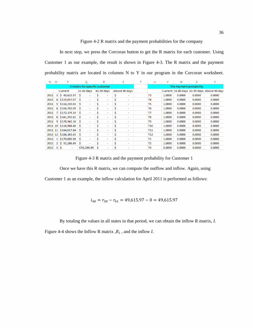
Figure 4-2 R matrix and the payment probabilities for the company ...................................... 36

Figure 4-3 R matrix and the payment probability for Customer 1 ........................................... 36

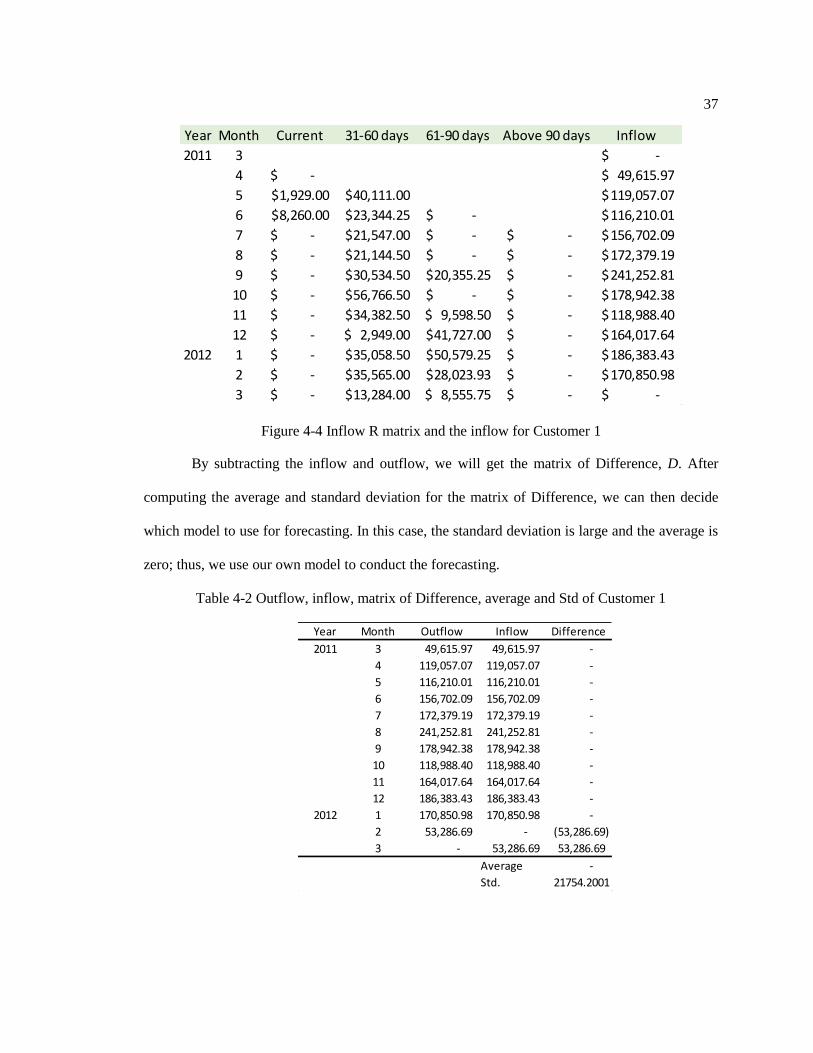
Figure 4-4 Inflow R matrix and the inflow for Customer 1 ..................................................... 37

vii

Figure 4-5 Forecast result for Customer 1 in April 2012 ......................................................... 38

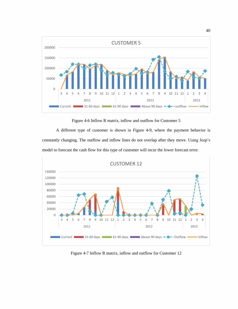
Figure 4-6 Inflow R matrix, inflow and outflow for Customer 5 ............................................ 40

Figure 4-7 Inflow R matrix, inflow and outflow for Customer 12 .......................................... 40

Figure 4-8 Forecast accuracy for Customer 1 .......................................................................... 46

Figure 4-9 Forecast accuracy for Customer 2 .......................................................................... 47

Figure 4-10 Forecast accuracy for Customer 3 ........................................................................ 47

Figure 4-11 Forecast accuracy for Customer 4 ........................................................................ 48

Figure 4-12 Forecast accuracy for Customer 5 ........................................................................ 48

Figure 4-13 Forecast accuracy for Customer 6 ........................................................................ 49

Figure 4-14 Forecast accuracy for Customer 7 ........................................................................ 49

Figure 4-15 Forecast accuracy for Customer 8 ........................................................................ 50

Figure 4-16 Forecast accuracy for Customer 9 ........................................................................ 50

Figure 4-17 Forecast accuracy for Customer 10 ...................................................................... 51

Figure 4-18 Forecast accuracy for Customer 11 ...................................................................... 51

Figure 4-19 Forecast accuracy for Customer 12 ..................................................................... 52

viii

LIST OF TABLES

Table 3-1. Relationship between day and state ........................................................................ 7

Table 3-2. Accounts Receivable Aging and States in Markov Chain ...................................... 10

Table 3-3. The calculation process for the AR aging matrix (R) ............................................ 11

Table 3-4 Faster method of copying and pasting ..................................................................... 32

Table 3-5 WITH statement ...................................................................................................... 32

Table 4-1 Difference between Models in the Program ............................................................ 34

Table 4-2 Outflow, inflow, matrix of Difference, average and Std of Customer 1 ................. 37

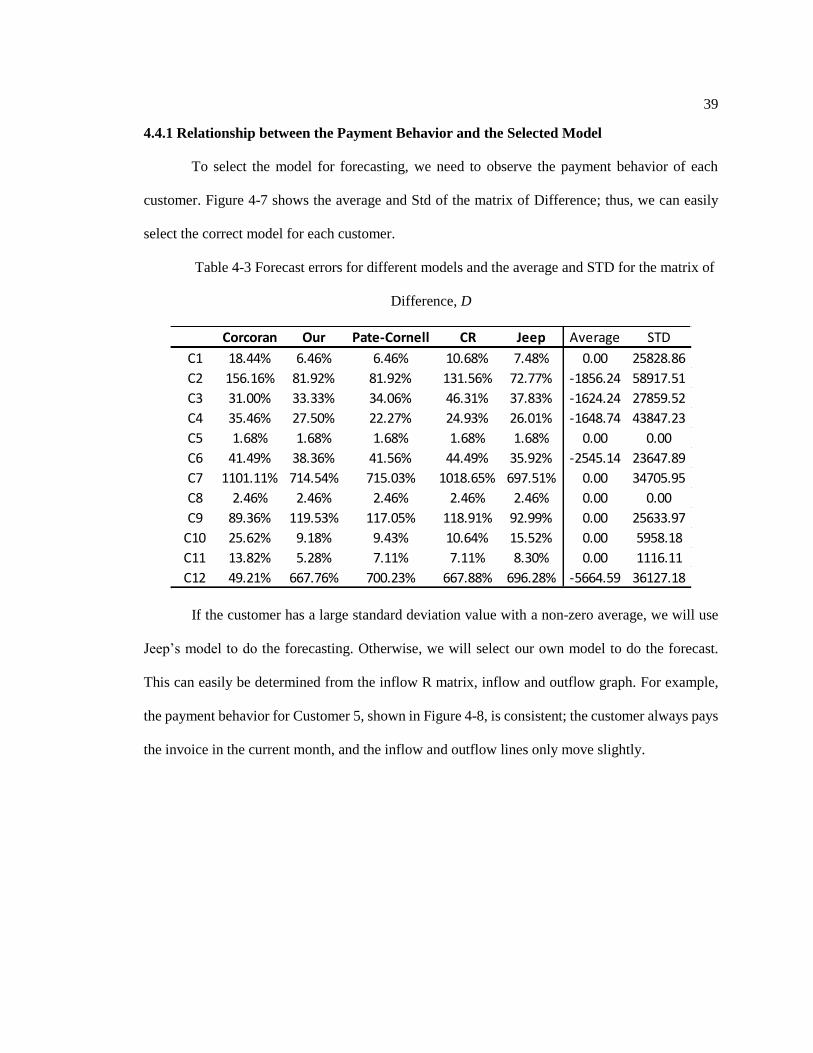
Table 4-3 Forecast errors for different models and the average and STD for the matrix of

Difference, D .................................................................................................................... 39

Table 4-4 Cash flow and forecasting difference for the entire company ................................. 41

Table 4-5 Cash flow and forecasting difference for the entire company ................................. 42

Table 4-6 Forecast accuracy for Corcoran model .................................................................... 43

Table 4-7 Forecast accuracy for Our model ............................................................................. 43

Table 4-8 Forecast accuracy for Pate-Cornell model ............................................................... 44

Table 4-9 Forecast accuracy for CR model ............................................................................. 44

Table 4-10 Forecast accuracy for Jeep model .......................................................................... 45

Table 4-11 Forecast accuracy for Combine model .................................................................. 45

Table 4-12 Confidence interval for six models ........................................................................ 46

Table 4-13 Confidence interval for 12 Customers ................................................................... 52

ix

Acknowledgements

I would like to thank Dr. Prabhu for his patience, professional guidance and care. I learned

a lot from doing this research. Without my advisor’s understanding and encouragement, I would

not have got this far in my research.

I would like to thank Dr. Yuncheol Kang, who offered a lot of advice, discussion and

support. Each time we discussed something, I always found the loophole in my thoughts. Thus, I

learned and improved a lot during the research.

I would like to thank Sunny Abann; without discussing and working with you, I might not

have finished this by the end of the semester. Thank you for cheering me up and for our discussions;

they helped me a lot during the research.

Finally, I would like to thank my parents, my brother and my friends for their love and

support, and for always standing by me during both good and bad times.

1

Chapter 1

Introduction

1.1 Background and Motivation

During difficulties in the economy, a good estimation of the collectability of account

receivables can make the difference between a company’s survival and its failure (Saibeni, 2010).

Two major factors may be the high and volatile rates and the increased competition for funds in the

consumer and trade credit market ( Kallberg, J. G. and Saunders, A., 1983). Especially for small

and medium-sized firms, due to their high credit risk, the interest rates for them are comparatively

higher than for the big companies (Baas, T. and Schrooten, M. , 2006). Because of this more

uncertain and competitive environment, the need for more effective cash flow forecasting is critical

to researchers and managers.

1.2 Research and Objectives

Our research starts from the stochastic financial analytics model (Tangsucheeva, R. and V.

Prabhu, 2014). First, we recreated the model and ran an empirical dataset, which we obtained from

a small company. After programming the model, we studied customer payment behavior and the

parameters in the result for each month. The objective of this thesis is to find the relationship

between the forecast model and customer payment behavior. We aimed to create a model that has

better forecasting results than Tangsucheeva’s model, and to classify the customers, based on their

payment behavior.

2

1.3 Outline of the Thesis

A literature review related to the subject will be provided in Chapter 2. First, we present

a discussion of cash flow management, cash flow forecasting, and cash flow risk. The previous

approach and concerns in this area will be shown, as well as an explanation of why this is

important. Then we will present the basis for this thesis.

In Chapter 3 the problem will be stated precisely. The model that we created will be

proposed, and each step of our methodology will be shown. We will discuss the assumption in

our model, and then illustrate the concept and the process of the entire model. Having provided

the outline, we will provide more in-depth details. We start by explaining how the forecast

model was selected by studying the payment behavior of each customer, and then we explain

the refined model from Jeep – which is the model proposed in this paper - in detail. Next we

will reveal the code for some important parts of the model and will discuss some key points

that are particularly noteworthy.

Then we will input the empirical data into our new model and show the results, as well

as the comparison with the previous model, in Chapter 4. We will introduce the data set and

implement the model using the data set introduced. Following this, we will show the results of

the implementation, including the forecast accuracy and the confidence interval. Finally, we

will present our conclusions regarding the implementation of this data set.

In Chapter 5 we present the conclusions on our model and discuss the limitations of

its forecasting ability. Also, we offer some directions for further research.

3

Chapter 2

LITERATURE REVIEW

2.1 Cash Flow Management

Cash flow management is concerned with the efficient use of the company's cash and short-

term investments (Gregory, 1976). The majority of models deal with a combination of three

decision types: cash position management; short-term investment; and short-term borrowing

(Srinivasan, V. and Kim, Y.H., 1986; Paulo S. F. Barbosa and Priscilla R. Pimentel, 2001). In the

supply chain, most of the approaches are based on the product flow, such as inventory and work in

process. A limited number of the models focus on the financial flow.

The earliest attempt was made by Baumol (Baumol, 1952), who viewed cash as an

inventory item. However, the model that he proposed is a deterministic model with the interest rate

and transfer fee to be constant, while the cash inflows and cash outflows were assumed to be

predetermined. Then Patinkin removed some of the objections to Baumol’s model (Patinkin, 1965).

He proposed the idea that the invoice and the payment may not be implemented in a systematic

way; thus, the balance of the cash flow would be negative. Then Miller and Orr (1966) removed

the restriction of a finite time zone and the cash flows were generated by a stationary Gaussian

random walk.

Another approach may be taken from the perspective of improving the Cash Conversion

Cycle (CCC) (Tsai, 2008) or by using the linear programming method (Barbosa, P.S.F. and

Pimentel, P.R., 2001). This mathematical programming is applied in the construction industry.

Cash flow management is essential for maximizing the value of the company. If the value

of the account receivables increases, then the value of the company decreases, due to the increase

4

in the cost of holding and the working capital (Michalski, 2007). Thus, the collection of account

receivables is a tradeoff between the risk of delayed payment and acquiring new customers.

2.2 Cash Flow Forecasting

The two categories of cash flow forecasting are: 1. Traditional – this estimates all the invoices

and the expenses over the schedule period; and 2. Statistic – this is often used to detect abnormal

performance (Srinivasan, V. and Kim, Y.H., 1986).

Most implementations are shown in forecasting the cash flow of a project, especially in the

construction industry. The time horizon for one case may be very long, and the total amount may be

quite large; thus, there are different methods for forecasting (Hwee, N. G. and Tiong R. L. K., 2002;

Skitmore, 1992). In the paper of Hwee and Tiong, the model measured five risk factors – including

duration, over/ under-measurement risk, variation risk, and material cost variances – and observed

their impact on the cash flow. Skitmore’s paper implemented the DHSS formula to obtain the best

parameter value. Once the combination of the best parameters is acquired, it can be applied to a

project that has a similar size, and similar results can be obtained.

Some approaches are taken from the perspective of accounts receivable. The generalized

model (Gentry, J.A. and De La Garza, J. M., 1985) is an extension of the CM model (Carpenter, M.

D. and Miller, J. E., 1979). It measures the collection, sales and joint effects that underlie changes

in accounts receivable, which means that it can explain the changes of amounts in the account

receivables. As in Stone’s model (Stone, 1976), the payment pattern is characterized by the

proportion of credit sales in a given month. Kallberg and Saunders (1983) based their work on the

CDT model (Cyert, R. M., Davidson, H. J. et al., 1962).

5

2.3 Basis for This Thesis

This thesis is an extension of the work presented in Tangsucheeva’s PhD dissertation. He

developed a stochastic financial analytics model by combining two models from Corcoran

(Corcoran, 1978) and Pate-Cornell (Pate-Cornell, M. E., Tagaras, G. et al., 1990). The former is

viewed as capturing the movement of the entire environment for the forecast, while the latter is

viewed as an individual movement. The model assumes that the Alpha and Beta values will

converge as the information increases. For the new customer, the forecast can be done by setting

the Beta value to one, which is the baseline environment.

This thesis considers the payment behavior of each customer, not only changing the shape

parameter in the Weibull distribution, but based on the payment behavior, we selected a different

model to conduct the forecast.

6

Chapter 3

STOCHASTIC FINANCIAL ANALYTICS FOR CASH FLOW

FORECASTING

3.1 Problem Statement

First we rebuilt the stochastic financial analytics mode (Tangsucheeva, R. and Prabhu, V.,

2014) l as our baseline. Then we focused on the changes in the customers’ payment behavior. The

objective of the thesis was to improve the stochastic financial analytics model with a lower margin

of forecasting error when customer behavior changes.

3.2 Methodology

In this section, we first explain the assumptions used for our model. Then we will explain

the model concept and the process flow. The forecast method that we created is a combined model

using two methods; Jeep’s model (Tangsucheeva, R. and Prabhu, V., 2014) and our own model.

Based on the payment behavior of the customer, we used a different method to conduct the forecast.

Finally, our model is explained in detail. Based on this model, we propose a computational

algorithm for better capturing the changes in customer behavior over time.

3.2.1 Assumptions

In the proposed algorithm, we assume that:

1. We have at least two months of historical data for each customer. The number of invoices

in each month is not limited, but the starting month should have at least one invoice.

2. The calculation of the average number of days to pay is calculated as follows:

7

Average days to pay = invoice pay date − invoice sent out day + 1

One extra day is added in this formula because we found that some invoices are paid on

the same day as they are sent out. Without adding an extra one into the calculation of the

average number of days to pay, this kind of payment behavior would be ignored.

3. The starting month for each customer can be different, and the invoices are not limited to

time sequences. This means that the customer might have invoices in one month, but no

invoices in the following month, or in two months’ time.

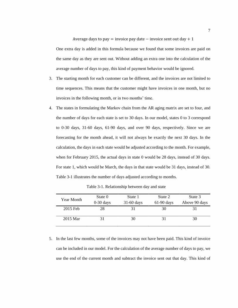
4. The states in formulating the Markov chain from the AR aging matrix are set to four, and

the number of days for each state is set to 30 days. In our model, states 0 to 3 correspond

to 0-30 days, 31-60 days, 61-90 days, and over 90 days, respectively. Since we are

forecasting for the month ahead, it will not always be exactly the next 30 days. In the

calculation, the days in each state would be adjusted according to the month. For example,

when for February 2015, the actual days in state 0 would be 28 days, instead of 30 days.

For state 1, which would be March, the days in that state would be 31 days, instead of 30.

Table 3-1 illustrates the number of days adjusted according to months.

Table 3-1. Relationship between day and state

Year Month State 0

0-30 days

State 1

31-60 days

State 2

61-90 days

State 3

Above 90 days

2015 Feb 28 31 30 31

2015 Mar 31 30 31 30

5. In the last few months, some of the invoices may not have been paid. This kind of invoice

can be included in our model. For the calculation of the average number of days to pay, we

use the end of the current month and subtract the invoice sent out that day. This kind of

8

invoice would be checked each month according to whether it is paid or not; we are not

merely handling historical data.

6. In the AR matrix, State 3 is seen as the bad debt. This cell would add up all the invoices

that have not been paid from the very beginning to that time slot. This would be checked

each month as well.

7. The payment probability at the first month in the AR matrix is the same as the payment

probability for the first calculation. For calculating the payment probability, two months’

invoice data are needed. The payment probability is calculated for the latest month of the

two, which means that there is no payment probability for the first month. For matching

the month with the Bayesian model, we set the first month’s payment probability to be the

same as the first calculation.

8. The payment probability of the first exponentially smoothed matrix for each state is the

average probability in the transition matrix of the same state.

9. The payment behavior for the forecasting month is the same as we calculated for this

month.

3.2.2 Model Concept and Process

The basis for our model was viewed by the company. For each month that the invoices

were sent out, the invoices were sorted according to the company name. The invoices were inputted

into the R matrix, and the inflow and outflow graphs were computed to observe the payment

probability. Based on the payment behavior, the decision was made as to which model should be

used for the forecasting. Finally, the total forecast for each company in this month was calculated

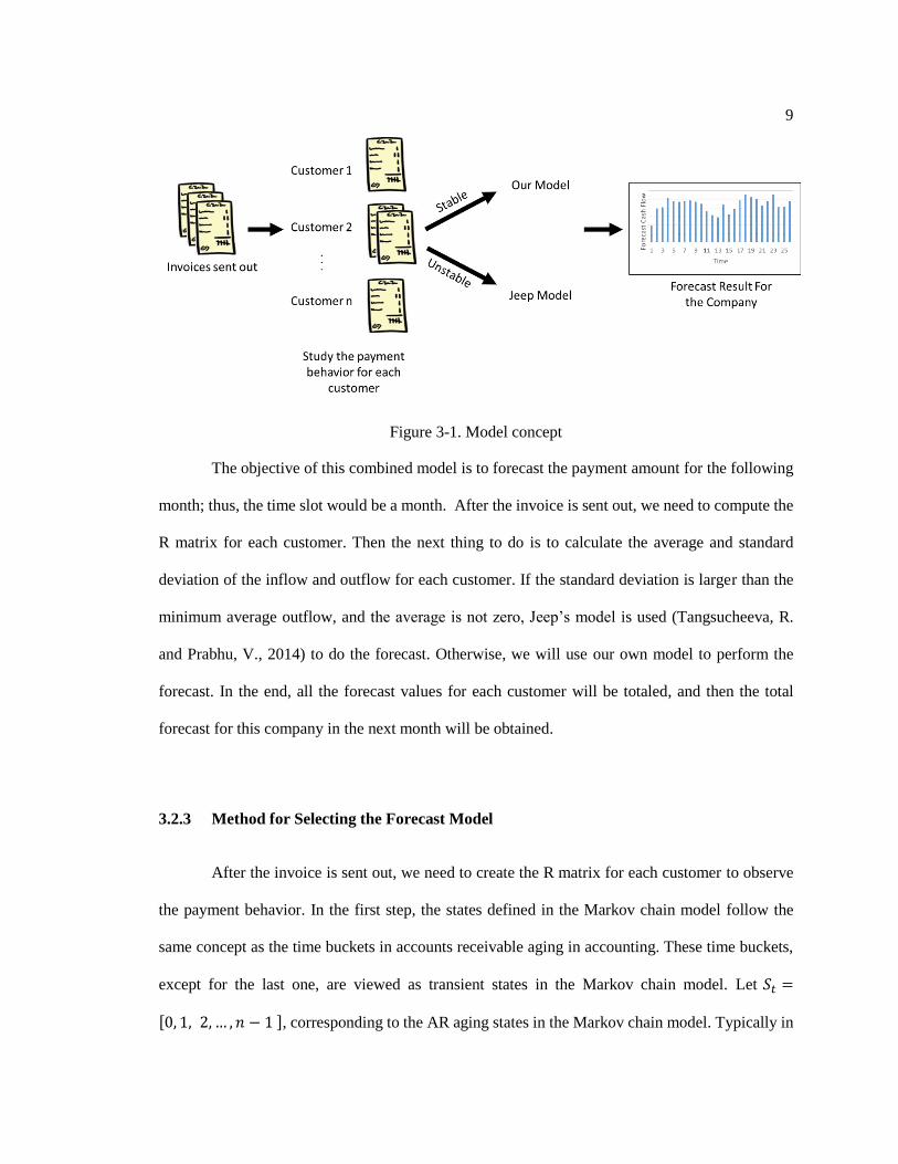
to reveal the forecast cash flow for this month. The model concept is summarized in Figure 3-1.

9

Figure 3-1. Model concept

The objective of this combined model is to forecast the payment amount for the following

month; thus, the time slot would be a month. After the invoice is sent out, we need to compute the

R matrix for each customer. Then the next thing to do is to calculate the average and standard

deviation of the inflow and outflow for each customer. If the standard deviation is larger than the

minimum average outflow, and the average is not zero, Jeep’s model is used (Tangsucheeva, R.

and Prabhu, V., 2014) to do the forecast. Otherwise, we will use our own model to perform the

forecast. In the end, all the forecast values for each customer will be totaled, and then the total

forecast for this company in the next month will be obtained.

3.2.3 Method for Selecting the Forecast Model

After the invoice is sent out, we need to create the R matrix for each customer to observe

the payment behavior. In the first step, the states defined in the Markov chain model follow the

same concept as the time buckets in accounts receivable aging in accounting. These time buckets,

except for the last one, are viewed as transient states in the Markov chain model. Let 𝑆𝑡 =

[0, 1, 2, … , 𝑛 − 1 ], corresponding to the AR aging states in the Markov chain model. Typically in

10

practice, time buckets are 0-30 days old, 31-60 days old, 61-90 days old, and over 90 days old.

(Accounts Receivable Analysis, 2015), but the difference between our model and the actual AR

aging calculation is that the days for the states are not restricted to 30 days. In our model, the days

in the states are aligned to the actual days in each month. Thus, the cash flow forecast can be viewed

each month without the need for any transformation formula.

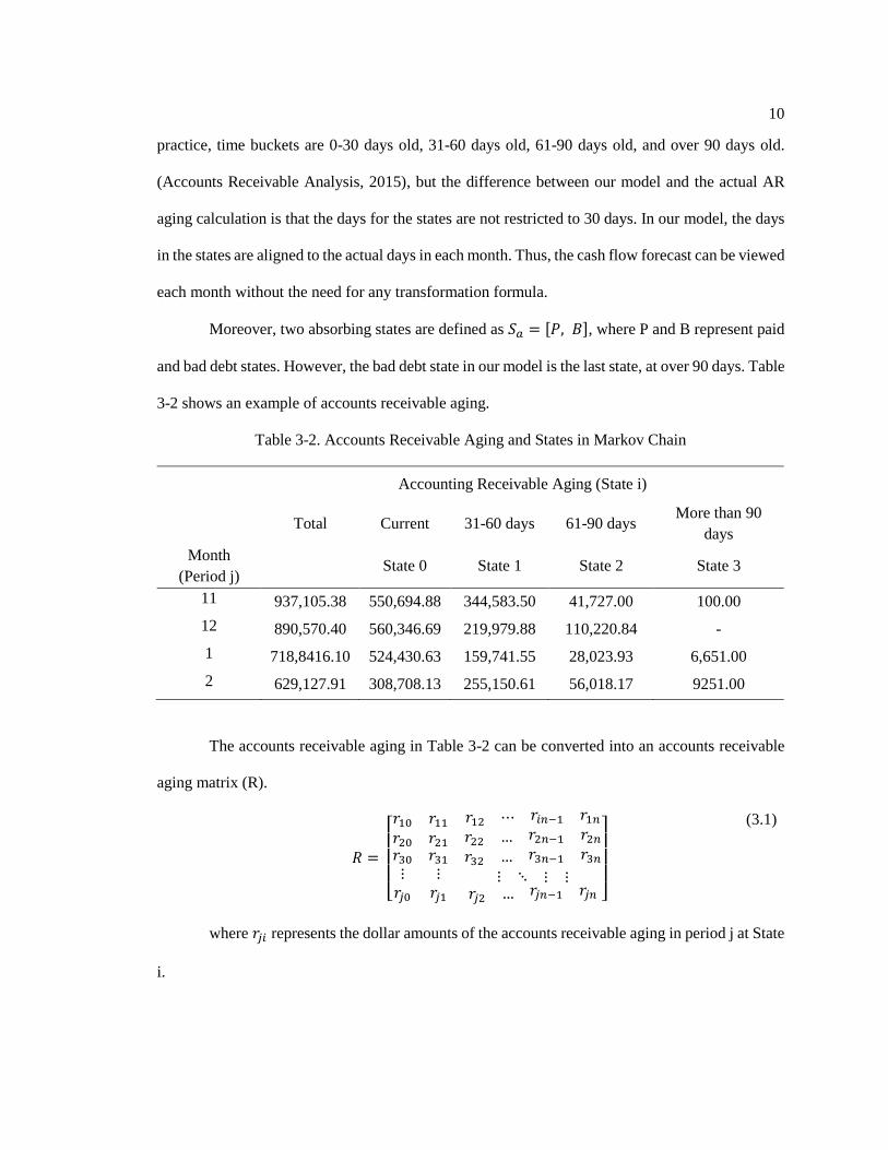
Moreover, two absorbing states are defined as 𝑆𝑎 = [𝑃, 𝐵], where P and B represent paid

and bad debt states. However, the bad debt state in our model is the last state, at over 90 days. Table

3-2 shows an example of accounts receivable aging.

Table 3-2. Accounts Receivable Aging and States in Markov Chain

Accounting Receivable Aging (State i)

Total Current 31-60 days 61-90 days

More than 90

days

Month

(Period j) State 0 State 1 State 2 State 3

11 937,105.38 550,694.88 344,583.50 41,727.00 100.00

12 890,570.40 560,346.69 219,979.88 110,220.84 -

1 718,8416.10 524,430.63 159,741.55 28,023.93 6,651.00

2 629,127.91 308,708.13 255,150.61 56,018.17 9251.00

The accounts receivable aging in Table 3-2 can be converted into an accounts receivable

aging matrix (R).

𝑅 =

[ 𝑟10 𝑟11 𝑟12 ⋯ 𝑟𝑖𝑛−1 𝑟1𝑛𝑟20 𝑟21 𝑟22 … 𝑟2𝑛−1 𝑟2𝑛𝑟30⋮𝑟𝑗0

𝑟31⋮𝑟𝑗1

𝑟32 … 𝑟3𝑛−1 𝑟3𝑛⋮ ⋱ ⋮ ⋮

𝑟𝑗2 … 𝑟𝑗𝑛−1 𝑟𝑗𝑛 ]

(3.1)

where 𝑟𝑗𝑖 represents the dollar amounts of the accounts receivable aging in period j at State

i.

11

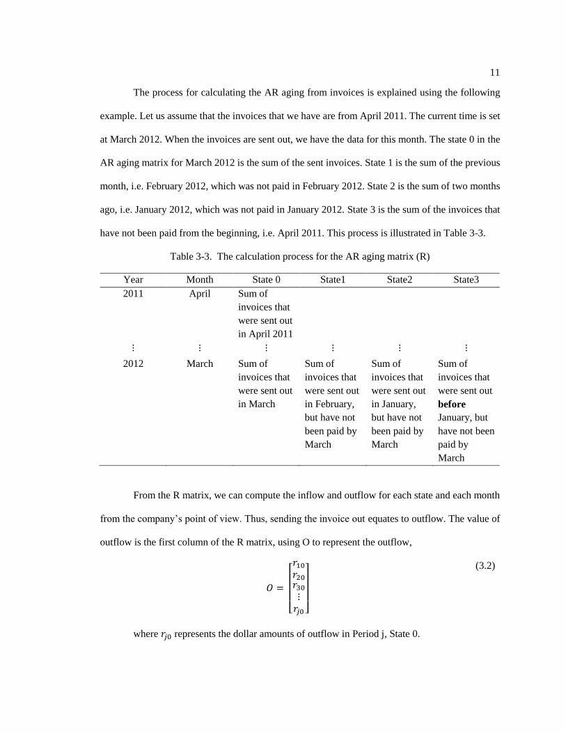
The process for calculating the AR aging from invoices is explained using the following

example. Let us assume that the invoices that we have are from April 2011. The current time is set

at March 2012. When the invoices are sent out, we have the data for this month. The state 0 in the

AR aging matrix for March 2012 is the sum of the sent invoices. State 1 is the sum of the previous

month, i.e. February 2012, which was not paid in February 2012. State 2 is the sum of two months

ago, i.e. January 2012, which was not paid in January 2012. State 3 is the sum of the invoices that

have not been paid from the beginning, i.e. April 2011. This process is illustrated in Table 3-3.

Table 3-3. The calculation process for the AR aging matrix (R)

Year Month State 0 State1 State2 State3

2011 April Sum of

invoices that

were sent out

in April 2011

⋮ ⋮ ⋮ ⋮ ⋮ ⋮

2012 March Sum of

invoices that

were sent out

in March

Sum of

invoices that

were sent out

in February,

but have not

been paid by

March

Sum of

invoices that

were sent out

in January,

but have not

been paid by

March

Sum of

invoices that

were sent out

before

January, but

have not been

paid by

March

From the R matrix, we can compute the inflow and outflow for each state and each month

from the company’s point of view. Thus, sending the invoice out equates to outflow. The value of

outflow is the first column of the R matrix, using O to represent the outflow,

𝑂 =

[ 𝑟10𝑟20𝑟30⋮𝑟𝑗0 ]

(3.2)

where 𝑟𝑗0 represents the dollar amounts of outflow in Period j, State 0.

12

The computation of inflow is similar to the idea of calculating the R matrix. The R matrix

represents the amount of money accounted for in invoices that have not been paid. Thus, by

subtracting the value in the R matrix we can see the amount that has been paid; that is how we

create an inflow R matrix, using 𝑅𝐼 to represent. Then we total the values in that period to get the

total inflow, using I to represent the inflow matrix,

𝑅𝐼 =

[ 0 0 0 ⋯ 0 0𝑖20 0 0 … 0 0𝑖30⋮𝑖𝑗0

𝑖31⋮𝑖𝑗1

0 … 0 0⋮ ⋱ ⋮ ⋮

𝑖𝑗2 … 𝑖𝑗𝑛−1 𝑖𝑗𝑛]

𝑖𝑗𝑛 = 𝑟𝑗−1,𝑛 − 𝑟𝑗,𝑛+1 (3.3)

where 𝑖𝑗𝑛 represents the dollar amounts of inflow in Period j, in State n. Since we only have

n states, the value for n+1 states are all set as zero.

By totaling the column values for each period, we will obtain the inflow for each state,

𝐼 =

[ 0𝑖2𝑖3⋮𝑖𝑗 ]

(3.4)

where 𝑖𝑗 represents the inflow amount in Period j.

The matrix of Difference, D, is computed by subtracting the inflow and outflow,

𝐷 =

[ 𝑑1𝑑2𝑑3⋮

𝑑𝑗−1]

𝑑𝑗−1 = 𝑟𝑗−1,0 − 𝑖𝑗 (3.5)

where 𝑑𝑗−1 is the difference in the cash flow in period j-1.

Once we have the D matrix, we can compute the average and the standard deviation for the

values in the D matrix. If the standard deviation is larger than the minimum average outflow for

13

each customer, and the average is not zero, then we will use Jeep’s model (Tangsucheeva, R. and

Prabhu, V., 2014) to perform the forecast. Otherwise, we will use our own model to do the forecast.

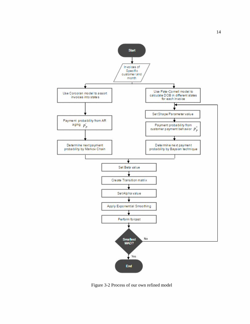
3.2.4 Process of Our Model

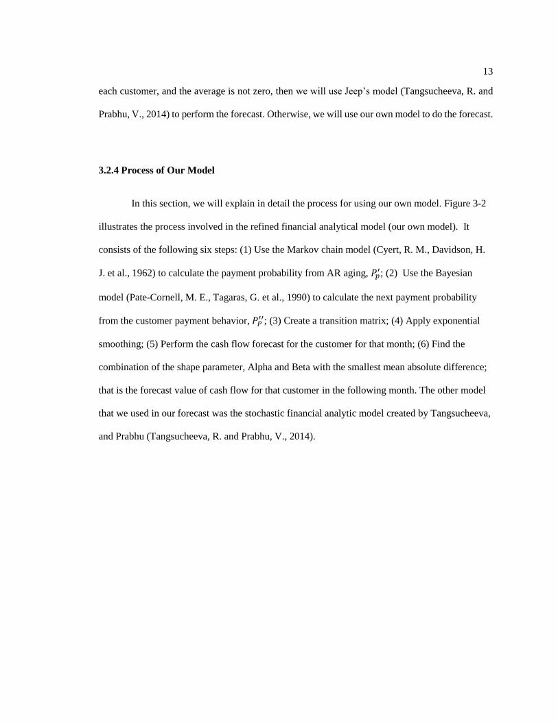
In this section, we will explain in detail the process for using our own model. Figure 3-2

illustrates the process involved in the refined financial analytical model (our own model). It

consists of the following six steps: (1) Use the Markov chain model (Cyert, R. M., Davidson, H.

J. et al., 1962) to calculate the payment probability from AR aging, 𝑃𝑝′; (2) Use the Bayesian

model (Pate-Cornell, M. E., Tagaras, G. et al., 1990) to calculate the next payment probability

from the customer payment behavior, 𝑃𝑃′′; (3) Create a transition matrix; (4) Apply exponential

smoothing; (5) Perform the cash flow forecast for the customer for that month; (6) Find the

combination of the shape parameter, Alpha and Beta with the smallest mean absolute difference;

that is the forecast value of cash flow for that customer in the following month. The other model

that we used in our forecast was the stochastic financial analytic model created by Tangsucheeva,

and Prabhu (Tangsucheeva, R. and Prabhu, V., 2014).

14

𝑃𝑃′

𝑃𝑃′′

Yes

No

Figure 3-2 Process of our own refined model

15

The first step in creating the R matrix is explained in Section 3.2.3. The only difference

between the R matrix in Section 3.2.3 and here is the input source. In Section 3.2.3, the input is a

specific customer, but in this section the matrix takes the company’s invoice as the input.

Once we have established the account receivable aging matrix, then we can determine the

𝑃𝑃′ from the changes from the previous month to this month (Corcoran, 1978),

𝑃𝑃′ =

[ 𝑃0𝑝′

𝑃1𝑃′

⋮𝑃𝑛𝑝′]

(3.6)

where

𝑃𝑖𝑃′ = (𝑟𝑗,𝑖 − 𝑟𝑗+1,𝑖+1)/𝑟𝑗,𝑖

(3.7)

where 𝑃𝑖𝑝′ is the payment probability from state i to state P (paid).

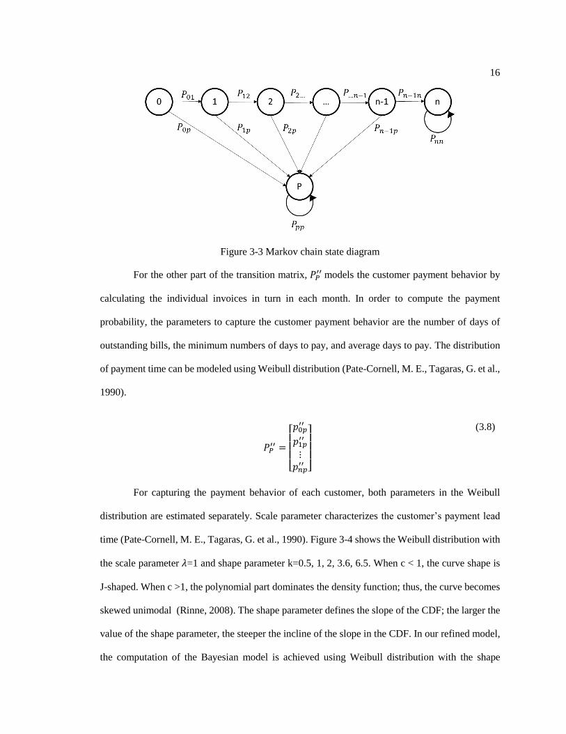
The elements in the 𝑃𝑃′ matrix indicate the transient states’ probability. Figure 3-3 shows

the Markov chain transition states and the probability. Every invoice in our model starts from State

0 (0-30 days), indicating the invoices that were sent out in the current month. If the invoice is not

paid in the current month, then it will transfer to the next month, and the probability will be

indicated as 𝑃01. Thus, the probability from State 0 to State P would be modeled as 𝑃0𝑝 = 1 − 𝑃1𝑝.

This will continue until it moves to the absorbing states, State P or State n, the state that we set as

bad debt in our model.

16

Figure 3-3 Markov chain state diagram

For the other part of the transition matrix, 𝑃𝑃′′ models the customer payment behavior by

calculating the individual invoices in turn in each month. In order to compute the payment

probability, the parameters to capture the customer payment behavior are the number of days of

outstanding bills, the minimum numbers of days to pay, and average days to pay. The distribution

of payment time can be modeled using Weibull distribution (Pate-Cornell, M. E., Tagaras, G. et al.,

1990).

𝑃𝑃′′ =

[ 𝑝0𝑝′′

𝑝1𝑝′′

⋮𝑝𝑛𝑝′′]

(3.8)

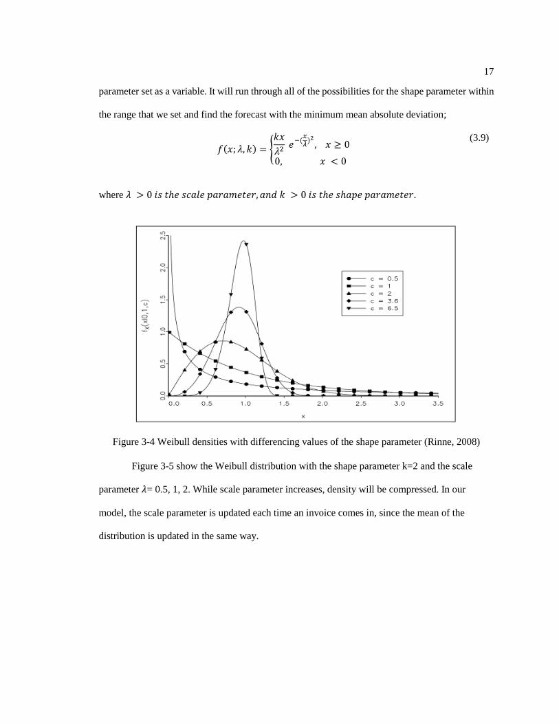
For capturing the payment behavior of each customer, both parameters in the Weibull

distribution are estimated separately. Scale parameter characterizes the customer’s payment lead

time (Pate-Cornell, M. E., Tagaras, G. et al., 1990). Figure 3-4 shows the Weibull distribution with

the scale parameter 𝜆=1 and shape parameter k=0.5, 1, 2, 3.6, 6.5. When c < 1, the curve shape is

J-shaped. When c >1, the polynomial part dominates the density function; thus, the curve becomes

skewed unimodal (Rinne, 2008). The shape parameter defines the slope of the CDF; the larger the

value of the shape parameter, the steeper the incline of the slope in the CDF. In our refined model,

the computation of the Bayesian model is achieved using Weibull distribution with the shape

17

parameter set as a variable. It will run through all of the possibilities for the shape parameter within

the range that we set and find the forecast with the minimum mean absolute deviation;

𝑓(𝑥; 𝜆, 𝑘) = {𝑘𝑥

𝜆2 𝑒

−(𝑥𝜆)2, 𝑥 ≥ 0

0, 𝑥 < 0

(3.9)

where 𝜆 > 0 𝑖𝑠 𝑡ℎ𝑒 𝑠𝑐𝑎𝑙𝑒 𝑝𝑎𝑟𝑎𝑚𝑒𝑡𝑒𝑟, 𝑎𝑛𝑑 𝑘 > 0 𝑖𝑠 𝑡ℎ𝑒 𝑠ℎ𝑎𝑝𝑒 𝑝𝑎𝑟𝑎𝑚𝑒𝑡𝑒𝑟.

Figure 3-4 Weibull densities with differencing values of the shape parameter (Rinne, 2008)

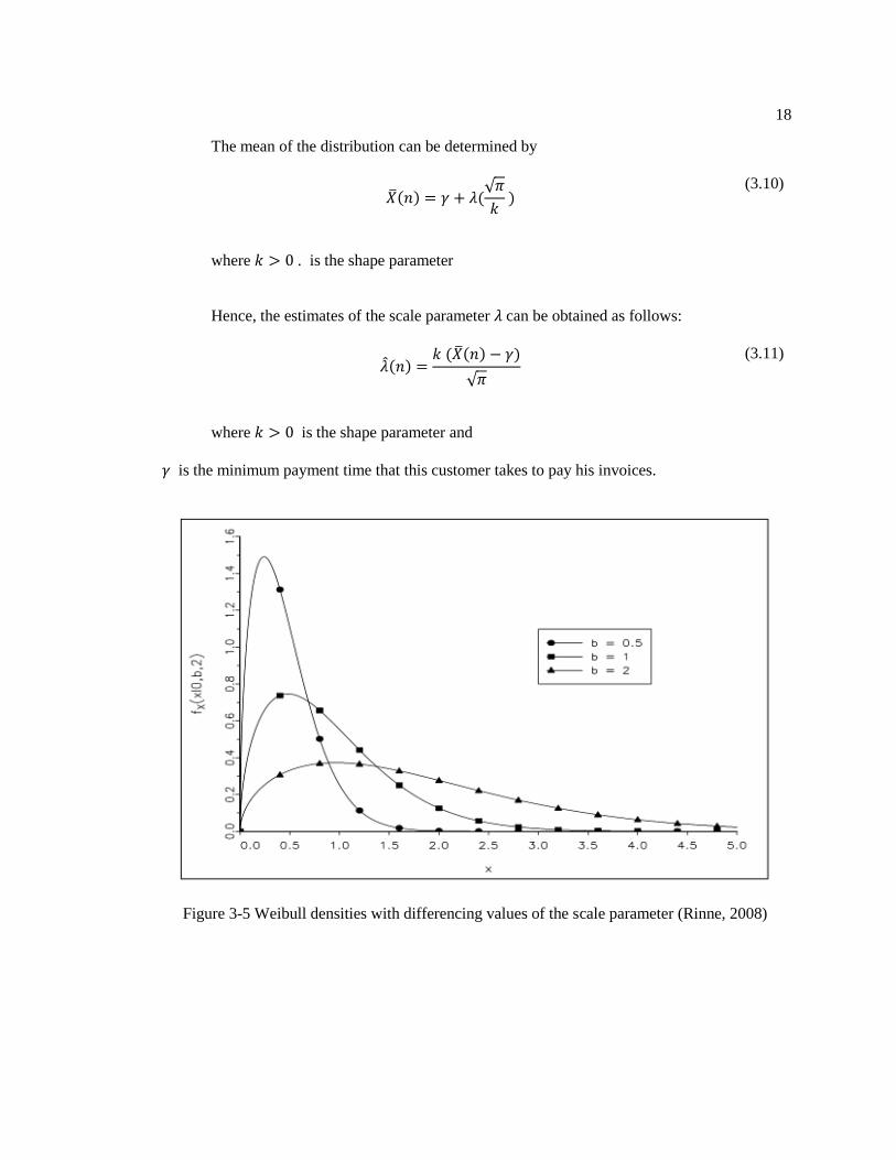
Figure 3-5 show the Weibull distribution with the shape parameter k=2 and the scale

parameter 𝜆= 0.5, 1, 2. While scale parameter increases, density will be compressed. In our

model, the scale parameter is updated each time an invoice comes in, since the mean of the

distribution is updated in the same way.

18

The mean of the distribution can be determined by

�̅�(𝑛) = 𝛾 + 𝜆(

√𝜋

𝑘 )

(3.10)

where 𝑘 > 0 . is the shape parameter

Hence, the estimates of the scale parameter 𝜆 can be obtained as follows:

�̂�(𝑛) =

𝑘 (�̅�(𝑛) − 𝛾)

√𝜋

(3.11)

where 𝑘 > 0 is the shape parameter and

𝛾 is the minimum payment time that this customer takes to pay his invoices.

Figure 3-5 Weibull densities with differencing values of the scale parameter (Rinne, 2008)

19

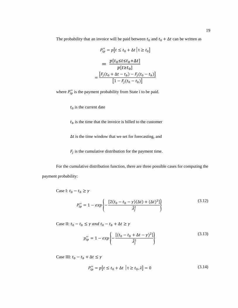
The probability that an invoice will be paid between 𝑡0 and 𝑡0 + Δ𝑡 can be written as

𝑃𝑖𝑝′′ = 𝑝[𝑡 ≤ 𝑡0 + Δ𝑡│t ≥ 𝑡0]

= 𝑝[𝑡0≤𝑡≤𝑡0+Δ𝑡]

𝑝[𝑡≥𝑡0]

=[𝐹𝑗(𝑡0 + Δ𝑡 − 𝑡𝑏) − 𝐹𝑗(𝑡0 − 𝑡𝑏)]

[1 − 𝐹𝑗(𝑡0 − 𝑡𝑏)]

where 𝑃𝑖𝑝′′ is the payment probability from State i to be paid.

𝑡0 is the current date

𝑡𝑏 is the time that the invoice is billed to the customer

Δt is the time window that we set for forecasting, and

𝐹𝑗 is the cumulative distribution for the payment time.

For the cumulative distribution function, there are three possible cases for computing the

payment probability:

Case I: 𝑡0 − 𝑡𝑏 ≥ 𝛾

𝑃𝑖𝑝′′ = 1 − 𝑒𝑥𝑝 {−

[2(𝑡0 − 𝑡𝑏 − 𝛾)(Δ𝑡) + (Δ𝑡)2]

�̂�𝑗2

} (3.12)

Case II: 𝑡0 − 𝑡𝑏 ≤ 𝛾 𝑎𝑛𝑑 𝑡0 − 𝑡𝑏 + Δ𝑡 ≥ 𝛾

𝑝𝑖𝑝′′ = 1 − 𝑒𝑥𝑝 {−

[(𝑡0 − 𝑡𝑏 + Δ𝑡 − 𝛾)2]

�̂�𝑗2

} (3.13)

Case III: 𝑡0 − 𝑡𝑏 + Δ𝑡 ≤ 𝛾

𝑃𝑖𝑝′′ = 𝑝[𝑡 ≤ 𝑡0 + Δ𝑡 │t ≥ 𝑡0, 𝜆] = 0 (3.14)

20

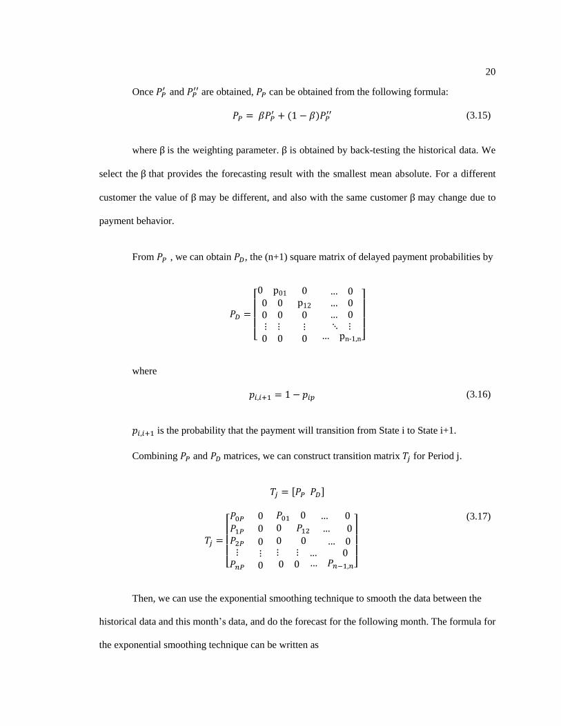
Once 𝑃𝑃′ and 𝑃𝑃

′′ are obtained, 𝑃𝑃 can be obtained from the following formula:

𝑃𝑃 = 𝛽𝑃𝑃′ + (1 − 𝛽)𝑃𝑃

′′ (3.15)

where β is the weighting parameter. β is obtained by back-testing the historical data. We

select the β that provides the forecasting result with the smallest mean absolute. For a different

customer the value of β may be different, and also with the same customer β may change due to

payment behavior.

From 𝑃𝑃 , we can obtain 𝑃𝐷, the (n+1) square matrix of delayed payment probabilities by

𝑃𝐷 =

[ 0 p01 0 … 00 0 p12 … 00 0⋮ ⋮0 0

0⋮0

… 0⋱ ⋮

… pn-1,n]

where

𝑝𝑖,𝑖+1 = 1 − 𝑝𝑖𝑝 (3.16)

𝑝𝑖,𝑖+1 is the probability that the payment will transition from State i to State i+1.

Combining 𝑃𝑃 and 𝑃𝐷 matrices, we can construct transition matrix 𝑇𝑗 for Period j.

𝑇𝑗 = [𝑃𝑃 𝑃𝐷]

𝑇𝑗 =

[ 𝑃0𝑃 0 𝑃01 0 … 0

𝑃1𝑃 0 0 𝑃12 … 0𝑃2𝑃⋮

𝑃𝑛𝑃

0⋮0

0 0 … 0⋮ ⋮ … 0 0 0 … 𝑃𝑛−1,𝑛]

(3.17)

Then, we can use the exponential smoothing technique to smooth the data between the

historical data and this month’s data, and do the forecast for the following month. The formula for

the exponential smoothing technique can be written as

21

𝐴�̅� = 𝛼𝑇𝑗 + (1 − 𝛼)𝐴𝑗−1̅̅ ̅̅ ̅̅ (3.18)

where

𝐴�̅� is the estimated transition matrix or exponentially smoothed matrix for Period j

𝛼 is the smoothing factor, and

𝑇𝑗 is the transition matrix for period j.

The smoothed factor is identified by running every number that we set within a range.

We take the forecast that has the smallest mean absolute deviation value. Then the cash flow

forecast can be obtained by (Corcoran, 1978)

𝐹𝑗+1 = 𝑅𝑗�̅�𝑗

𝐹𝑗+1 = [𝑟𝑗0 𝑟𝑗1 𝑟𝑗2 … 𝑟𝑗𝑛]

[ 𝑝0𝑝 0 0 𝑝01 0 … 0

𝑝1𝑝 0 0 0 𝑝12 … 0

𝑝2𝑝⋮

𝑝𝑛𝑝

0⋮0

0 0 0 … 0

⋮ ⋮ ⋮ ⋱ ⋮ 0 0 0 … 𝑝𝑛−1,𝑛]

(3.19)

where

𝐹𝑗+1 is the cash flow forecast vector of each State for Period j+1, and

𝑅𝑗 is the vector of the actual account receivable in Period j from the R matrix.

By repeating this procedure to forecast for all of the customers, we can obtain the

company’s cash flow forecast.

22

3.3 Computation

We used Excel VBA 2013 (Visual Basic for Applications) to implement the refined model.

We chose this tool for two reasons: Firstly, approximately 70% of companies are using it for

accounting and cash flow forecasts (Fuchs, 2011); thus, using this tool makes it easier for

companies to master our model for forecasting. The second reason is that the built-in capabilities,

statistical analysis, and computation abilities are suitable for cash flow forecasting.

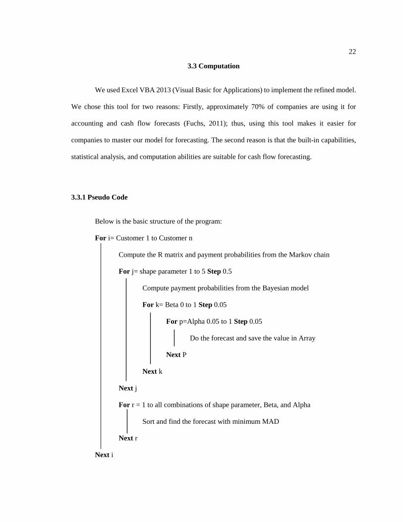
3.3.1 Pseudo Code

Below is the basic structure of the program:

For i= Customer 1 to Customer n

Compute the R matrix and payment probabilities from the Markov chain

For j= shape parameter 1 to 5 Step 0.5

Compute payment probabilities from the Bayesian model

For k= Beta 0 to 1 Step 0.05

For p=Alpha 0.05 to 1 Step 0.05

Do the forecast and save the value in Array

Next P

Next k

Next j

For r = 1 to all combinations of shape parameter, Beta, and Alpha

Sort and find the forecast with minimum MAD

Next r

Next i

23

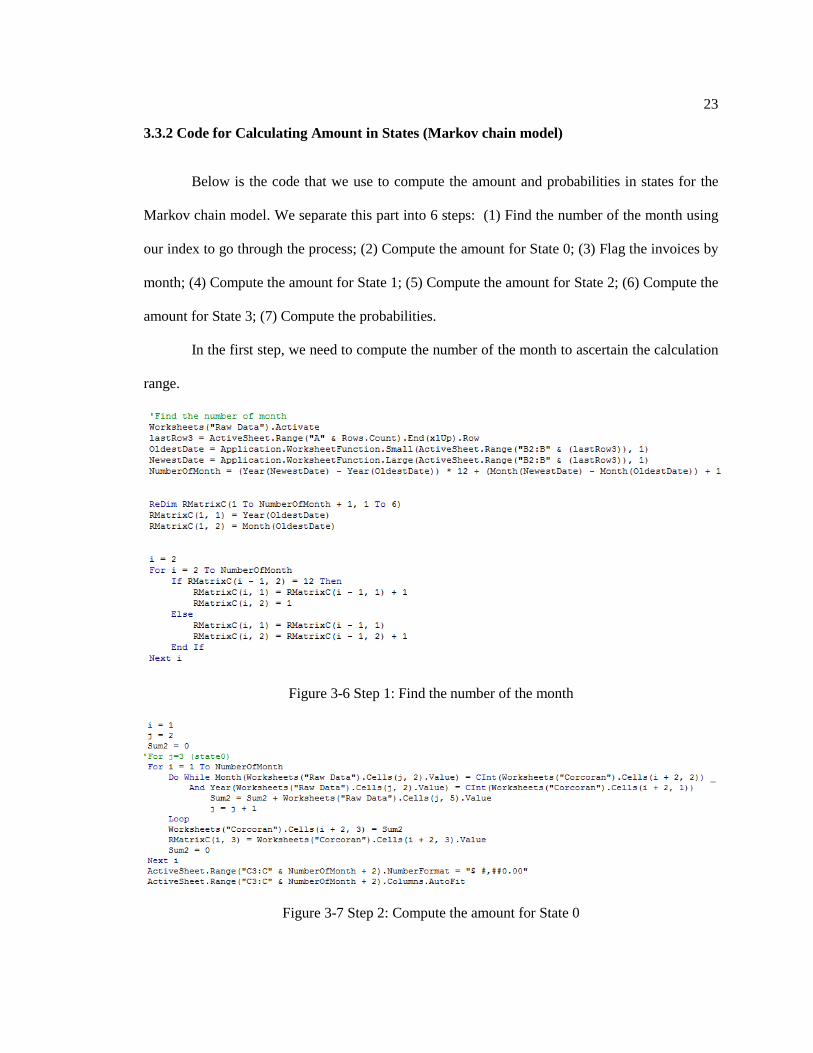
3.3.2 Code for Calculating Amount in States (Markov chain model)

Below is the code that we use to compute the amount and probabilities in states for the

Markov chain model. We separate this part into 6 steps: (1) Find the number of the month using

our index to go through the process; (2) Compute the amount for State 0; (3) Flag the invoices by

month; (4) Compute the amount for State 1; (5) Compute the amount for State 2; (6) Compute the

amount for State 3; (7) Compute the probabilities.

In the first step, we need to compute the number of the month to ascertain the calculation

range.

Figure 3-6 Step 1: Find the number of the month

Figure 3-7 Step 2: Compute the amount for State 0

24

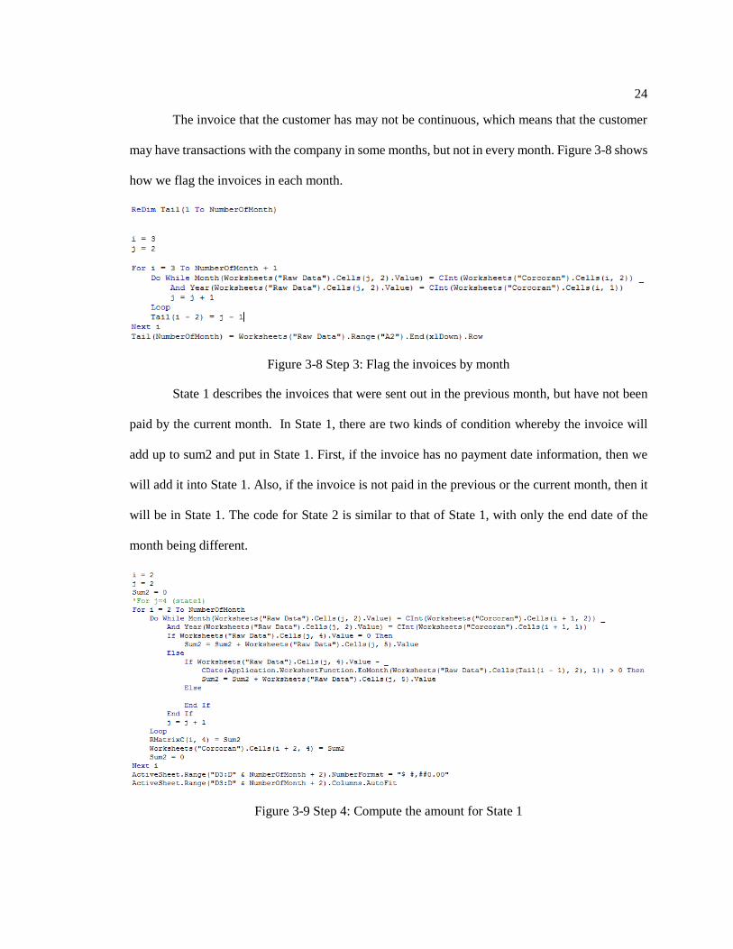
The invoice that the customer has may not be continuous, which means that the customer

may have transactions with the company in some months, but not in every month. Figure 3-8 shows

how we flag the invoices in each month.

Figure 3-8 Step 3: Flag the invoices by month

State 1 describes the invoices that were sent out in the previous month, but have not been

paid by the current month. In State 1, there are two kinds of condition whereby the invoice will

add up to sum2 and put in State 1. First, if the invoice has no payment date information, then we

will add it into State 1. Also, if the invoice is not paid in the previous or the current month, then it

will be in State 1. The code for State 2 is similar to that of State 1, with only the end date of the

month being different.

Figure 3-9 Step 4: Compute the amount for State 1

25

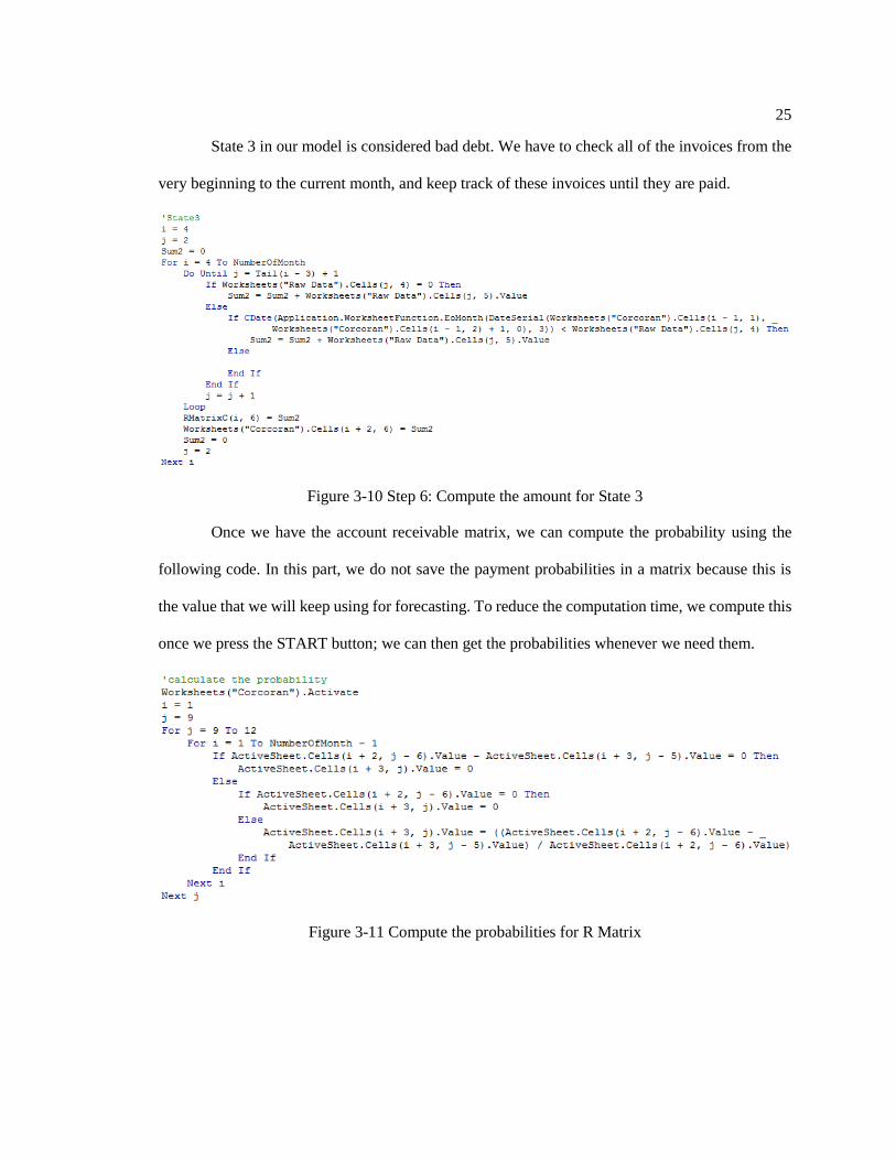
State 3 in our model is considered bad debt. We have to check all of the invoices from the

very beginning to the current month, and keep track of these invoices until they are paid.

Figure 3-10 Step 6: Compute the amount for State 3

Once we have the account receivable matrix, we can compute the probability using the

following code. In this part, we do not save the payment probabilities in a matrix because this is

the value that we will keep using for forecasting. To reduce the computation time, we compute this

once we press the START button; we can then get the probabilities whenever we need them.

Figure 3-11 Compute the probabilities for R Matrix

26

3.3.3 Code for Computing Days of Outstanding Bills and the Probabilities in Bayesian

Model

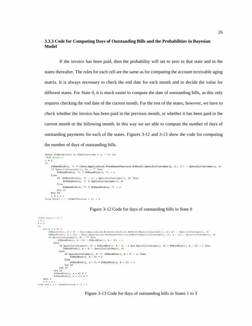
If the invoice has been paid, then the probability will set to zero in that state and in the

states thereafter. The rules for each cell are the same as for computing the account receivable aging

matrix. It is always necessary to check the end date for each month and to decide the value for

different states. For State 0, it is much easier to compute the date of outstanding bills, as this only

requires checking the end date of the current month. For the rest of the states, however, we have to

check whether the invoice has been paid in the previous month, or whether it has been paid in the

current month or the following month. In this way we are able to compute the number of days of

outstanding payments for each of the states. Figures 3-12 and 3-13 show the code for computing

the number of days of outstanding bills.

Figure 3-12 Code for days of outstanding bills in State 0

Figure 3-13 Code for days of outstanding bills in States 1 to 3

27

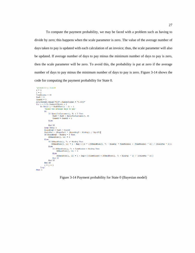
To compute the payment probability, we may be faced with a problem such as having to

divide by zero; this happens when the scale parameter is zero. The value of the average number of

days taken to pay is updated with each calculation of an invoice; thus, the scale parameter will also

be updated. If average number of days to pay minus the minimum number of days to pay is zero,

then the scale parameter will be zero. To avoid this, the probability is put at zero if the average

number of days to pay minus the minimum number of days to pay is zero. Figure 3-14 shows the

code for computing the payment probability for State 0.

Figure 3-14 Payment probability for State 0 (Bayesian model)

28

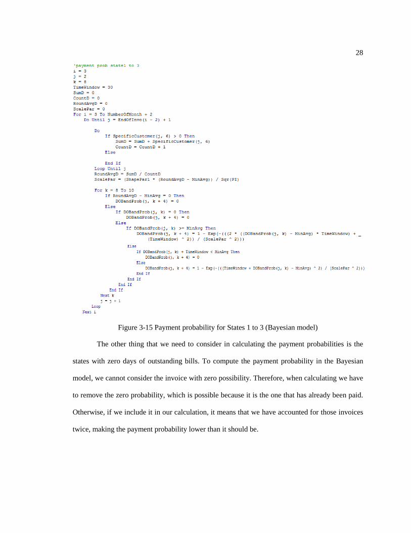
Figure 3-15 Payment probability for States 1 to 3 (Bayesian model)

The other thing that we need to consider in calculating the payment probabilities is the

states with zero days of outstanding bills. To compute the payment probability in the Bayesian

model, we cannot consider the invoice with zero possibility. Therefore, when calculating we have

to remove the zero probability, which is possible because it is the one that has already been paid.

Otherwise, if we include it in our calculation, it means that we have accounted for those invoices

twice, making the payment probability lower than it should be.

29

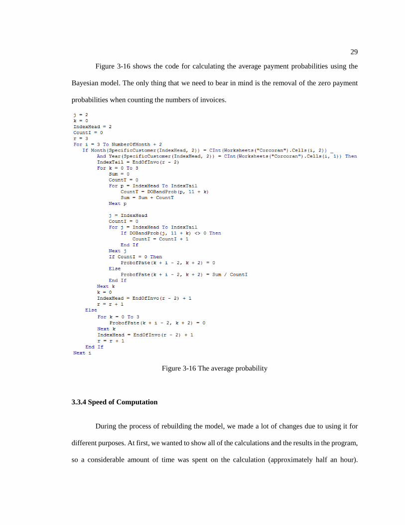
Figure 3-16 shows the code for calculating the average payment probabilities using the

Bayesian model. The only thing that we need to bear in mind is the removal of the zero payment

probabilities when counting the numbers of invoices.

Figure 3-16 The average probability

3.3.4 Speed of Computation

During the process of rebuilding the model, we made a lot of changes due to using it for

different purposes. At first, we wanted to show all of the calculations and the results in the program,

so a considerable amount of time was spent on the calculation (approximately half an hour).

30

However, when testing the data set, this kind of speed is not possible with this kind of size. Using

the first version of the program, it may take up to two days to receive all of the results. Thus, we

optimized our program to speed it up. The following are the rules that we used in the program:

1. Screen updating

The screen updating property controls the display of the changes on the monitor

while the program is running. This is considered dragging the speed, since it has to

read in and out every time after the calculation. Therefore, we can turn this property

off, and turn it back on at the end, and the result can still be retrieved and displayed.

We have to put the following command at the start of the code:

Application.ScreenUpdating = False

and put the command at the end of the code, before End Sub.

Application.ScreenUpdating = True

2. Minimize traffic between VBA and the worksheet

When handling the large data table in Excel, the processing of the data from the

worksheet and writing it back will slow down the execution of the code. Therefore,

instead of storing the data in the cell, they are stored in the memory, using an array. It

must be set as a dynamic array, and redeclared each time to clear the previous content.

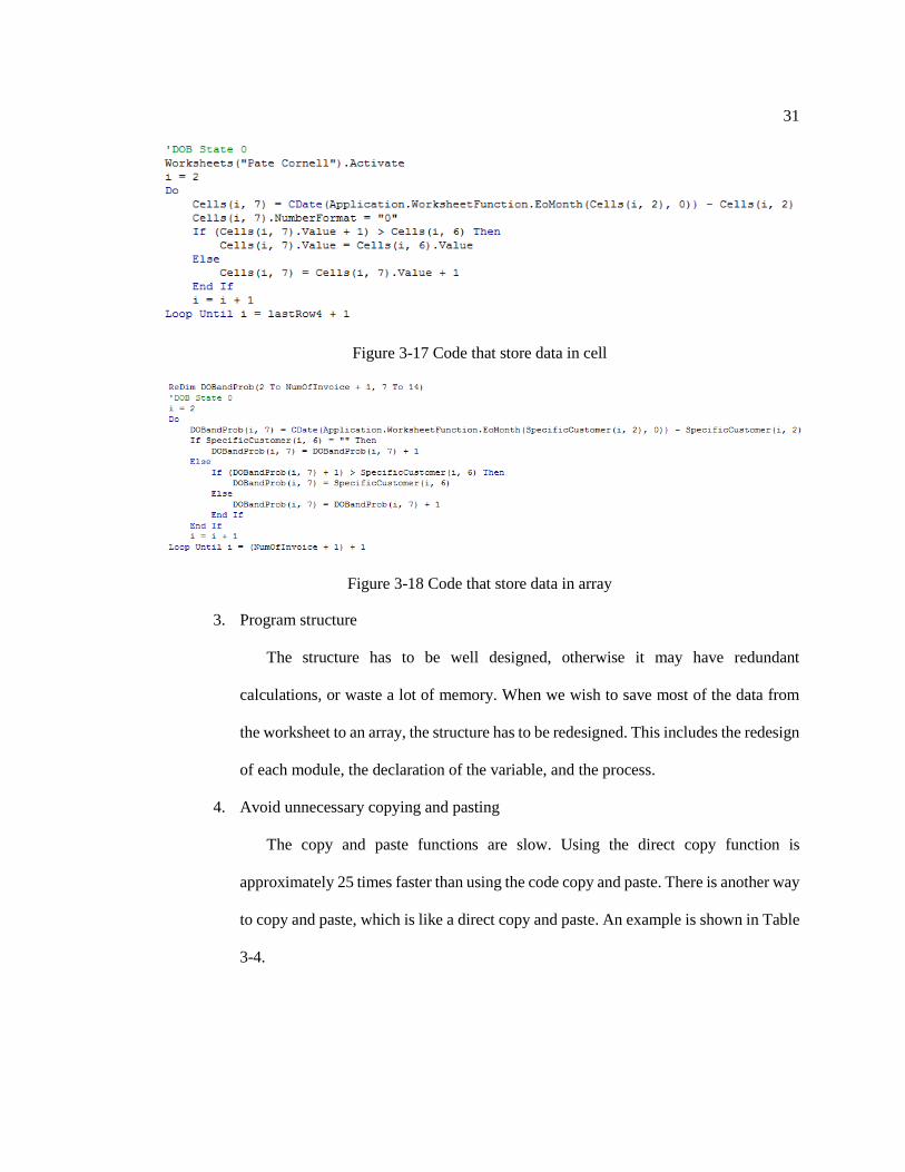
For example, Figures 3-16 and 3-17 show the code for computing the number of days

of outstanding bills in State 0, but the execution time shown in Figure 3-17 is smaller,

since the process can all be reread from the memory instead of requiring the worksheet

as well as the memory.

31

Figure 3-17 Code that store data in cell

Figure 3-18 Code that store data in array

3. Program structure

The structure has to be well designed, otherwise it may have redundant

calculations, or waste a lot of memory. When we wish to save most of the data from

the worksheet to an array, the structure has to be redesigned. This includes the redesign

of each module, the declaration of the variable, and the process.

4. Avoid unnecessary copying and pasting

The copy and paste functions are slow. Using the direct copy function is

approximately 25 times faster than using the code copy and paste. There is another way

to copy and paste, which is like a direct copy and paste. An example is shown in Table

3-4.

32

Table 3-4 Faster method of copying and pasting

Slow macro Fast macro

Worksheets(“1”).Range(“I4:L4”).Copy

Worksheets(“1”).Range(“I3:L3”).Paste

Worksheets(“1”).Range(“I4:L4”).Copy _

Destination: =

Worksheets(“1”).Range(“I3:L3”).

5. Specific data type declaration

The declaration of the object type affects the storage size. If the data is an integer,

it only uses 4 bytes. But without declaring the variable, it will be declared as variant

by default, which uses 16 bytes, four times more than the integer. Also, if you need to

process a large data set, the effect will be magnified. Thus, it is important to declare

the specific data type.

6. Avoid selecting objects

There is no need to select objects before working with them, but writing property

selection in the code will force excel to spend time selecting each object that is being

manipulated. This often shows in the recording macro or copy and paste.

7. WITH Statements

If we have to access the same object with different properties and methods many

times, we can use a WITH statement to avoid writing the fully qualified object path

repeatedly.

Table 3-5 WITH statement

Slow macro Fast macro

Sheet(1).Range(“I4:L4”).Font.Bold=True

Sheet(1).Range(“I4:L4”).Name=”Calibri”

Sheet(1).Range(“I4:L4”).Interior.ColorIndex=2

With Sheet(1).Range(“I4:L4”)

.Font.Bold=True

.Name=”Calibri”

Interior.ColorIndex=2

End with

33

8. Worksheet functions

In VBA, we can still use functions that are built in Excel, and of course VBA has

built-in functions. Most of them consume less system resources than if you build them

yourself.

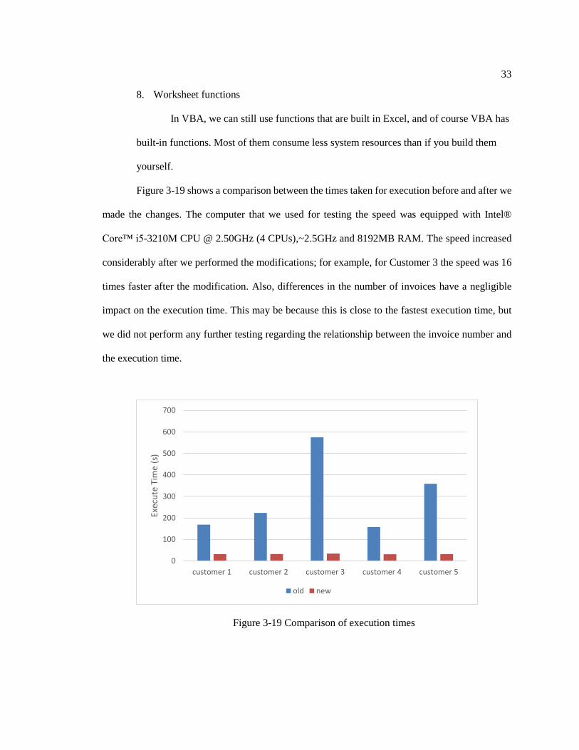
Figure 3-19 shows a comparison between the times taken for execution before and after we

made the changes. The computer that we used for testing the speed was equipped with Intel®

Core™ i5-3210M CPU @ 2.50GHz (4 CPUs),~2.5GHz and 8192MB RAM. The speed increased

considerably after we performed the modifications; for example, for Customer 3 the speed was 16

times faster after the modification. Also, differences in the number of invoices have a negligible

impact on the execution time. This may be because this is close to the fastest execution time, but

we did not perform any further testing regarding the relationship between the invoice number and

the execution time.

Figure 3-19 Comparison of execution times

0

100

200

300

400

500

600

700

customer 1 customer 2 customer 3 customer 4 customer 5

Exec

ute

Tim

e (s

)

old new

34

Chapter 4 Illustrative Example

In this chapter, an example is presented to illustrate the stochastic financial analytic model

developed in Chapter 3. The following input data is the same as in Tangsucheeva’s thesis

(Tangsucheeva, R. and Prabhu, V., 2014). The model was programmed using Excel VBA 2013

version (Visual Basic for Applications).

4.1 Input Data

The data set that we used was provided by a company with 12 different customers. The

period of the data set was from March 2011 to April 2013, totaling 26 months. The input required

for each invoice included: (1) Name of the customer; (2) Date that the invoice was sent out; (3) The

due date of the invoice; (4) Payment date of the invoice; (5) The amount of the invoice; and (6)

Number of days the invoice was outstanding.

4.2 Difference between Models in a Program

To illustrate the results of our model, we rebuilt the models described in Corcoran’s paper

(Corcoran, 1978), Pate-Cornell’s paper (Pate-Cornell, M. E., Tagaras, G., et al., 1990) and

Tangsucheeva’s thesis (Tangsucheeva, R. and Prabhu, V., 2014), abbreviated to Corcoran, Pate-

Cornell and Jeep. Also, our own intermediate model was used. Table 4-1 shows the parameters set

in the program.

Table 4-1 Difference between Models in the Program

Corcoran Specific Customer 1 Between 0.05-1 2

Our own Entire company Between 0-1 Between 0.05-1 Between 1~5

Pate-Cornell Entire company 0 Between 0.05-1 2

CR Specific Customer Between 0-1 Between 0.05-1 Between 1~5

35

Jeep Entire company Between 0-1 Between 0.05-1 2

4.3 Implementing the Model

In this section, we will detail our program step by step. Once we have the invoice

information, we can paste it into our program and then press the START button. In this way, we

will get the customer list in the same worksheet and the entire company’s R matrix in a

worksheet named Corcoran. Figure 4-1 shows the program interface of the starting page.

Figure 4-1 Inputting the data into our program

In the next worksheet, Corcoran, will show the company’s R matrix. Figure 4-2 shows

the format used in the program.

36

Figure 4-2 R matrix and the payment probabilities for the company

In next step, we press the Corcoran button to get the R matrix for each customer. Using

Customer 1 as our example, the result is shown in Figure 4-3. The R matrix and the payment

probability matrix are located in columns N to Y in our program in the Corcoran worksheet.

Figure 4-3 R matrix and the payment probability for Customer 1

Once we have this R matrix, we can compute the outflow and inflow. Again, using

Customer 1 as an example, the inflow calculation for April 2011 is performed as follows:

𝑖40 = 𝑟30 − 𝑟41 = 49,615.97 − 0 = 49,615.97

By totaling the values in all states in that period, we can obtain the inflow R matrix, I.

Figure 4-4 shows the Inflow R matrix ,𝑅𝐼 , and the inflow I.

37

Figure 4-4 Inflow R matrix and the inflow for Customer 1

By subtracting the inflow and outflow, we will get the matrix of Difference, D. After

computing the average and standard deviation for the matrix of Difference, we can then decide

which model to use for forecasting. In this case, the standard deviation is large and the average is

zero; thus, we use our own model to conduct the forecasting.

Table 4-2 Outflow, inflow, matrix of Difference, average and Std of Customer 1

Year Month Current 31-60 days 61-90 days Above 90 days Inflow

2011 3 -$

4 -$ 49,615.97$

5 1,929.00$ 40,111.00$ 119,057.07$

6 8,260.00$ 23,344.25$ -$ 116,210.01$

7 -$ 21,547.00$ -$ -$ 156,702.09$

8 -$ 21,144.50$ -$ -$ 172,379.19$

9 -$ 30,534.50$ 20,355.25$ -$ 241,252.81$

10 -$ 56,766.50$ -$ -$ 178,942.38$

11 -$ 34,382.50$ 9,598.50$ -$ 118,988.40$

12 -$ 2,949.00$ 41,727.00$ -$ 164,017.64$

2012 1 -$ 35,058.50$ 50,579.25$ -$ 186,383.43$

2 -$ 35,565.00$ 28,023.93$ -$ 170,850.98$

3 -$ 13,284.00$ 8,555.75$ -$ -$

Year Month Outflow Inflow Difference

2011 3 49,615.97 49,615.97 -

4 119,057.07 119,057.07 -

5 116,210.01 116,210.01 -

6 156,702.09 156,702.09 -

7 172,379.19 172,379.19 -

8 241,252.81 241,252.81 -

9 178,942.38 178,942.38 -

10 118,988.40 118,988.40 -

11 164,017.64 164,017.64 -

12 186,383.43 186,383.43 -

2012 1 170,850.98 170,850.98 -

2 53,286.69 - (53,286.69)

3 - 53,286.69 53,286.69

Average -

Std. 21754.2001

38

Then, by pressing our own model button in the starting page, we can get the forecast

value for Customer 1 for April 2012, as shown in Figure 4-6.

Figure 4-5 Forecast result for Customer 1 in April 2012

By repeating this process for all customers and finding the total, it is therefore possible to

obtain the cash flow forecast for the company for the following month.

4.4 Results and Discussion

In this section, we will first discuss the payment behavior and the cash inflow and outflow.

Then we will determine the type of forecast model that should be used for customer, using the

results that we have obtained. Next, we will compare the results across six different models from

two different perspectives. Finally, we will demonstrate the forecast accuracy and the confidence

interval for each customer.

39

4.4.1 Relationship between the Payment Behavior and the Selected Model

To select the model for forecasting, we need to observe the payment behavior of each

customer. Figure 4-7 shows the average and Std of the matrix of Difference; thus, we can easily

select the correct model for each customer.

Table 4-3 Forecast errors for different models and the average and STD for the matrix of

Difference, D

If the customer has a large standard deviation value with a non-zero average, we will use

Jeep’s model to do the forecasting. Otherwise, we will select our own model to do the forecast.

This can easily be determined from the inflow R matrix, inflow and outflow graph. For example,

the payment behavior for Customer 5, shown in Figure 4-8, is consistent; the customer always pays

the invoice in the current month, and the inflow and outflow lines only move slightly.

Corcoran Our Pate-Cornell CR Jeep Average STD

C1 18.44% 6.46% 6.46% 10.68% 7.48% 0.00 25828.86

C2 156.16% 81.92% 81.92% 131.56% 72.77% -1856.24 58917.51

C3 31.00% 33.33% 34.06% 46.31% 37.83% -1624.24 27859.52

C4 35.46% 27.50% 22.27% 24.93% 26.01% -1648.74 43847.23

C5 1.68% 1.68% 1.68% 1.68% 1.68% 0.00 0.00

C6 41.49% 38.36% 41.56% 44.49% 35.92% -2545.14 23647.89

C7 1101.11% 714.54% 715.03% 1018.65% 697.51% 0.00 34705.95

C8 2.46% 2.46% 2.46% 2.46% 2.46% 0.00 0.00

C9 89.36% 119.53% 117.05% 118.91% 92.99% 0.00 25633.97

C10 25.62% 9.18% 9.43% 10.64% 15.52% 0.00 5958.18

C11 13.82% 5.28% 7.11% 7.11% 8.30% 0.00 1116.11

C12 49.21% 667.76% 700.23% 667.88% 696.28% -5664.59 36127.18

40

Figure 4-6 Inflow R matrix, inflow and outflow for Customer 5

A different type of customer is shown in Figure 4-9, where the payment behavior is

constantly changing. The outflow and inflow lines do not overlap after they move. Using Jeep’s

model to forecast the cash flow for this type of customer will incur the lower forecast error.

Figure 4-7 Inflow R matrix, inflow and outflow for Customer 12

0

50000

100000

150000

200000

3 4 5 6 7 8 9 10 11 12 1 2 3 4 5 6 7 8 9 10 11 12 1 2 3 4

2011 2012 2013

CUSTOMER 5

Current 31-60 days 61-90 days Above 90 days outflow Inflow

0

20000

40000

60000

80000

100000

120000

140000

3 4 5 6 7 8 9 10 11 12 1 2 3 4 5 6 7 8 9 10 11 12 1 2 3 4

2011 2012 2013

CUSTOMER 12

Current 31-60 days 61-90 days Above 90 days Outflow Inflow

41

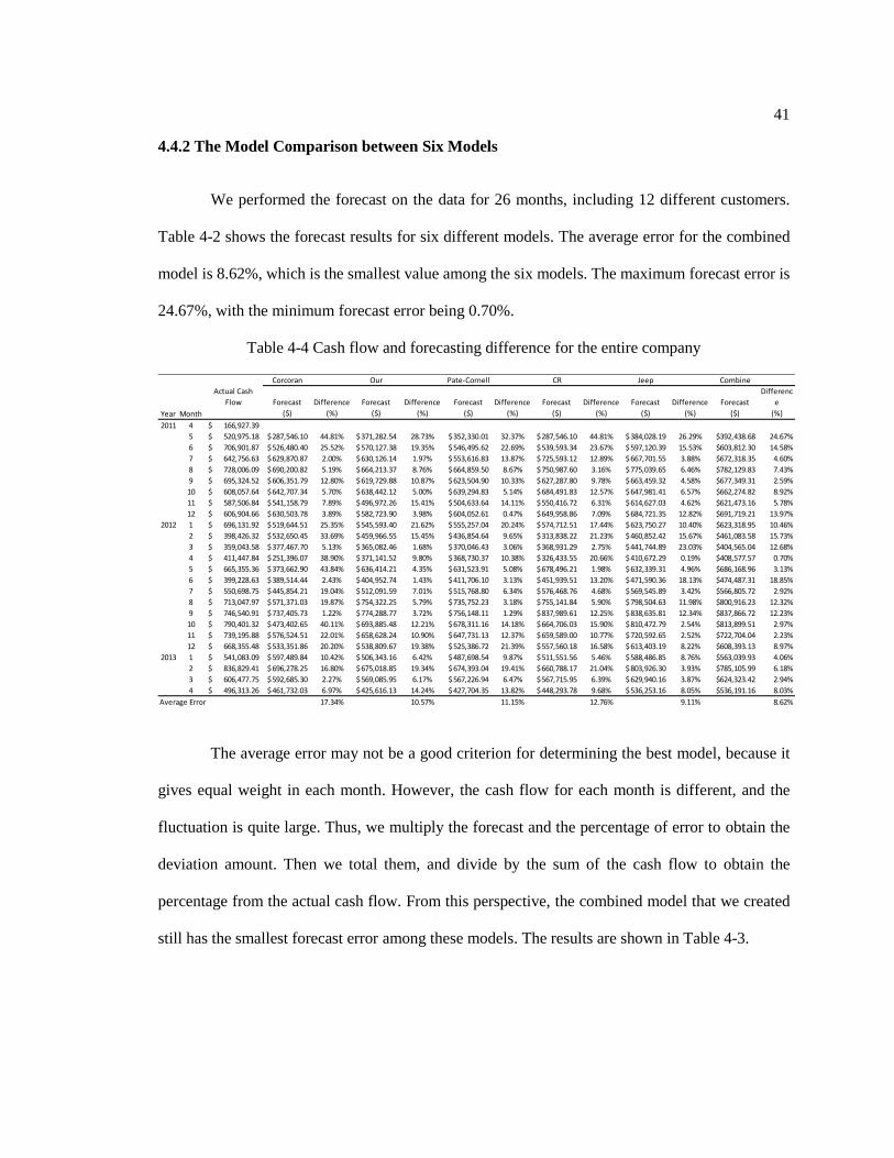
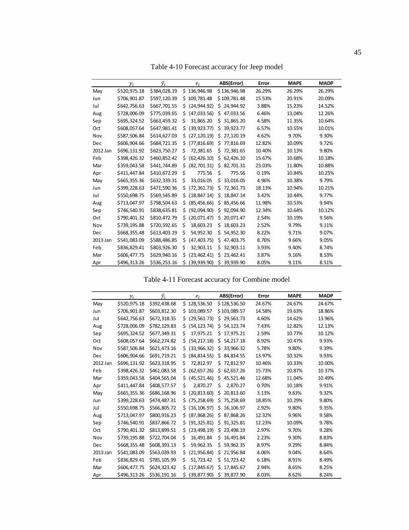
4.4.2 The Model Comparison between Six Models

We performed the forecast on the data for 26 months, including 12 different customers.

Table 4-2 shows the forecast results for six different models. The average error for the combined

model is 8.62%, which is the smallest value among the six models. The maximum forecast error is

24.67%, with the minimum forecast error being 0.70%.

Table 4-4 Cash flow and forecasting difference for the entire company

The average error may not be a good criterion for determining the best model, because it

gives equal weight in each month. However, the cash flow for each month is different, and the

fluctuation is quite large. Thus, we multiply the forecast and the percentage of error to obtain the

deviation amount. Then we total them, and divide by the sum of the cash flow to obtain the

percentage from the actual cash flow. From this perspective, the combined model that we created

still has the smallest forecast error among these models. The results are shown in Table 4-3.

Corcoran Our Pate-Cornell CR Jeep Combine

Year Month

Forecast

($)

Difference

(%)

Forecast

($)

Difference

(%)

Forecast

($)

Difference

(%)

Forecast

($)

Difference

(%)

Forecast

($)

Difference

(%)

Forecast

($)

Differenc

e

(%)

2011 4 166,927.39$

5 520,975.18$ 287,546.10$ 44.81% 371,282.54$ 28.73% 352,330.01$ 32.37% 287,546.10$ 44.81% 384,028.19$ 26.29% $392,438.68 24.67%

6 706,901.87$ 526,480.40$ 25.52% 570,127.38$ 19.35% 546,495.62$ 22.69% 539,593.34$ 23.67% 597,120.39$ 15.53% $603,812.30 14.58%

7 642,756.63$ 629,870.87$ 2.00% 630,126.14$ 1.97% 553,616.83$ 13.87% 725,593.12$ 12.89% 667,701.55$ 3.88% $672,318.35 4.60%

8 728,006.09$ 690,200.82$ 5.19% 664,213.37$ 8.76% 664,859.50$ 8.67% 750,987.60$ 3.16% 775,039.65$ 6.46% $782,129.83 7.43%

9 695,324.52$ 606,351.79$ 12.80% 619,729.88$ 10.87% 623,504.90$ 10.33% 627,287.80$ 9.78% 663,459.32$ 4.58% $677,349.31 2.59%

10 608,057.64$ 642,707.34$ 5.70% 638,442.12$ 5.00% 639,294.83$ 5.14% 684,491.83$ 12.57% 647,981.41$ 6.57% $662,274.82 8.92%

11 587,506.84$ 541,158.79$ 7.89% 496,972.26$ 15.41% 504,633.64$ 14.11% 550,416.72$ 6.31% 614,627.03$ 4.62% $621,473.16 5.78%

12 606,904.66$ 630,503.78$ 3.89% 582,723.90$ 3.98% 604,052.61$ 0.47% 649,958.86$ 7.09% 684,721.35$ 12.82% $691,719.21 13.97%

2012 1 696,131.92$ 519,644.51$ 25.35% 545,593.40$ 21.62% 555,257.04$ 20.24% 574,712.51$ 17.44% 623,750.27$ 10.40% $623,318.95 10.46%

2 398,426.32$ 532,650.45$ 33.69% 459,966.55$ 15.45% 436,854.64$ 9.65% 313,838.22$ 21.23% 460,852.42$ 15.67% $461,083.58 15.73%

3 359,043.58$ 377,467.70$ 5.13% 365,082.46$ 1.68% 370,046.43$ 3.06% 368,931.29$ 2.75% 441,744.89$ 23.03% $404,565.04 12.68%

4 411,447.84$ 251,396.07$ 38.90% 371,141.52$ 9.80% 368,730.37$ 10.38% 326,433.55$ 20.66% 410,672.29$ 0.19% $408,577.57 0.70%

5 665,355.36$ 373,662.90$ 43.84% 636,414.21$ 4.35% 631,523.91$ 5.08% 678,496.21$ 1.98% 632,339.31$ 4.96% $686,168.96 3.13%

6 399,228.63$ 389,514.44$ 2.43% 404,952.74$ 1.43% 411,706.10$ 3.13% 451,939.51$ 13.20% 471,590.36$ 18.13% $474,487.31 18.85%

7 550,698.75$ 445,854.21$ 19.04% 512,091.59$ 7.01% 515,768.80$ 6.34% 576,468.76$ 4.68% 569,545.89$ 3.42% $566,805.72 2.92%

8 713,047.97$ 571,371.03$ 19.87% 754,322.25$ 5.79% 735,752.23$ 3.18% 755,141.84$ 5.90% 798,504.63$ 11.98% $800,916.23 12.32%

9 746,540.91$ 737,405.73$ 1.22% 774,288.77$ 3.72% 756,148.11$ 1.29% 837,989.61$ 12.25% 838,635.81$ 12.34% $837,866.72 12.23%

10 790,401.32$ 473,402.65$ 40.11% 693,885.48$ 12.21% 678,311.16$ 14.18% 664,706.03$ 15.90% 810,472.79$ 2.54% $813,899.51 2.97%

11 739,195.88$ 576,524.51$ 22.01% 658,628.24$ 10.90% 647,731.13$ 12.37% 659,589.00$ 10.77% 720,592.65$ 2.52% $722,704.04 2.23%

12 668,355.48$ 533,351.86$ 20.20% 538,809.67$ 19.38% 525,386.72$ 21.39% 557,560.18$ 16.58% 613,403.19$ 8.22% $608,393.13 8.97%

2013 1 541,083.09$ 597,489.84$ 10.42% 506,343.16$ 6.42% 487,698.54$ 9.87% 511,551.56$ 5.46% 588,486.85$ 8.76% $563,039.93 4.06%

2 836,829.41$ 696,278.25$ 16.80% 675,018.85$ 19.34% 674,393.04$ 19.41% 660,788.17$ 21.04% 803,926.30$ 3.93% $785,105.99 6.18%

3 606,477.75$ 592,685.30$ 2.27% 569,085.95$ 6.17% 567,226.94$ 6.47% 567,715.95$ 6.39% 629,940.16$ 3.87% $624,323.42 2.94%

4 496,313.26$ 461,732.03$ 6.97% 425,616.13$ 14.24% 427,704.35$ 13.82% 448,293.78$ 9.68% 536,253.16$ 8.05% $536,191.16 8.03%

Average Error 17.34% 10.57% 11.15% 12.76% 9.11% 8.62%

Actual Cash

Flow

42

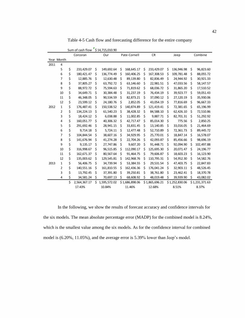
Table 4-5 Cash flow and forecasting difference for the entire company

In the following, we show the results of forecast accuracy and confidence intervals for

the six models. The mean absolute percentage error (MADP) for the combined model is 8.24%,

which is the smallest value among the six models. As for the confidence interval for combined

model is (6.20%, 11.05%), and the average error is 5.39% lower than Jeep’s model.

Sum of cash flow 14,715,010.90$

Corcoran Our Pate-Cornell CR Jeep Combine

Year Month

2011 4

5 233,429.07$ 149,692.64$ 168,645.17$ 233,429.07$ 136,946.98$ 96,823.60$

6 180,421.47$ 136,774.49$ 160,406.25$ 167,308.53$ 109,781.48$ 88,055.72$

7 12,885.76$ 12,630.48$ 89,139.80$ 82,836.49$ 24,944.92$ 30,921.33$

8 37,805.27$ 63,792.72$ 63,146.60$ 22,981.51$ 47,033.56$ 58,147.57$

9 88,972.72$ 75,594.63$ 71,819.62$ 68,036.72$ 31,865.20$ 17,510.52$

10 34,649.71$ 30,384.48$ 31,237.19$ 76,434.19$ 39,923.77$ 59,051.43$

11 46,348.05$ 90,534.59$ 82,873.21$ 37,090.12$ 27,120.19$ 35,930.06$

12 23,599.12$ 24,180.76$ 2,852.05$ 43,054.19$ 77,816.69$ 96,667.33$

2012 1 176,487.41$ 150,538.52$ 140,874.89$ 121,419.41$ 72,381.65$ 65,196.99$

2 134,224.13$ 61,540.23$ 38,428.32$ 84,588.10$ 62,426.10$ 72,510.86$

3 18,424.12$ 6,038.88$ 11,002.85$ 9,887.71$ 82,701.31$ 51,292.92$

4 160,051.77$ 40,306.32$ 42,717.47$ 85,014.30$ 775.56$ 2,850.25$

5 291,692.46$ 28,941.15$ 33,831.45$ 13,140.85$ 33,016.05$ 21,464.69$

6 9,714.18$ 5,724.11$ 12,477.48$ 52,710.89$ 72,361.73$ 89,445.72$

7 104,844.54$ 38,607.16$ 34,929.95$ 25,770.01$ 18,847.14$ 16,578.07$

8 141,676.94$ 41,274.28$ 22,704.26$ 42,093.87$ 85,456.66$ 98,696.19$

9 9,135.17$ 27,747.86$ 9,607.20$ 91,448.71$ 92,094.90$ 102,497.88$

10 316,998.67$ 96,515.85$ 112,090.17$ 125,695.30$ 20,071.47$ 24,196.77$

11 162,671.37$ 80,567.64$ 91,464.75$ 79,606.87$ 18,603.23$ 16,123.90$

12 135,003.62$ 129,545.81$ 142,968.76$ 110,795.31$ 54,952.30$ 54,582.76$

2013 1 56,406.75$ 34,739.94$ 53,384.55$ 29,531.54$ 47,403.75$ 22,847.83$

2 140,551.16$ 161,810.55$ 162,436.36$ 176,041.24$ 32,903.11$ 48,526.45$

3 13,792.45$ 37,391.80$ 39,250.81$ 38,761.80$ 23,462.41$ 18,370.78$

4 34,581.24$ 70,697.13$ 68,608.92$ 48,019.48$ 39,939.90$ 43,082.02$

2,564,367.17$ 1,595,572.02$ 1,686,898.06$ 1,865,696.21$ 1,252,830.06$ 1,231,371.63$

17.43% 10.84% 11.46% 12.68% 8.51% 8.37%

43

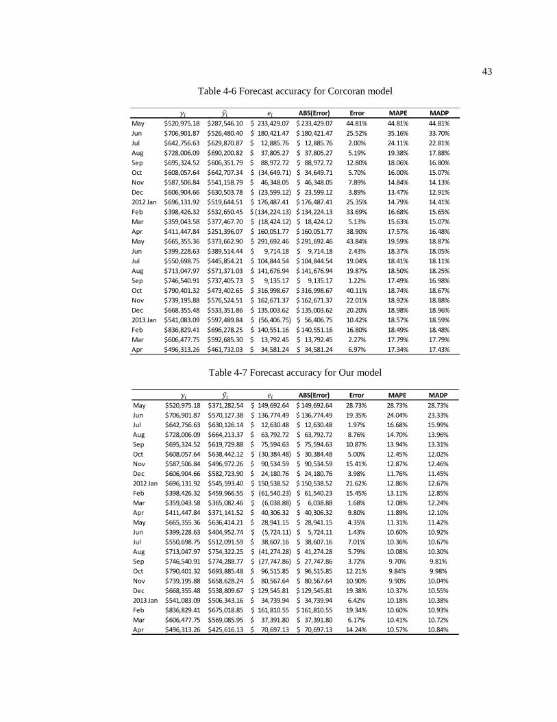
Table 4-6 Forecast accuracy for Corcoran model

Table 4-7 Forecast accuracy for Our model

ABS(Error) Error MAPE MADP

May 520,975.18$ 287,546.10$ 233,429.07$ 233,429.07$ 44.81% 44.81% 44.81%

Jun 706,901.87$ 526,480.40$ 180,421.47$ 180,421.47$ 25.52% 35.16% 33.70%

Jul 642,756.63$ 629,870.87$ 12,885.76$ 12,885.76$ 2.00% 24.11% 22.81%

Aug 728,006.09$ 690,200.82$ 37,805.27$ 37,805.27$ 5.19% 19.38% 17.88%

Sep 695,324.52$ 606,351.79$ 88,972.72$ 88,972.72$ 12.80% 18.06% 16.80%

Oct 608,057.64$ 642,707.34$ (34,649.71)$ 34,649.71$ 5.70% 16.00% 15.07%

Nov 587,506.84$ 541,158.79$ 46,348.05$ 46,348.05$ 7.89% 14.84% 14.13%

Dec 606,904.66$ 630,503.78$ (23,599.12)$ 23,599.12$ 3.89% 13.47% 12.91%

2012 Jan 696,131.92$ 519,644.51$ 176,487.41$ 176,487.41$ 25.35% 14.79% 14.41%

Feb 398,426.32$ 532,650.45$ (134,224.13)$ 134,224.13$ 33.69% 16.68% 15.65%

Mar 359,043.58$ 377,467.70$ (18,424.12)$ 18,424.12$ 5.13% 15.63% 15.07%

Apr 411,447.84$ 251,396.07$ 160,051.77$ 160,051.77$ 38.90% 17.57% 16.48%

May 665,355.36$ 373,662.90$ 291,692.46$ 291,692.46$ 43.84% 19.59% 18.87%

Jun 399,228.63$ 389,514.44$ 9,714.18$ 9,714.18$ 2.43% 18.37% 18.05%

Jul 550,698.75$ 445,854.21$ 104,844.54$ 104,844.54$ 19.04% 18.41% 18.11%

Aug 713,047.97$ 571,371.03$ 141,676.94$ 141,676.94$ 19.87% 18.50% 18.25%

Sep 746,540.91$ 737,405.73$ 9,135.17$ 9,135.17$ 1.22% 17.49% 16.98%

Oct 790,401.32$ 473,402.65$ 316,998.67$ 316,998.67$ 40.11% 18.74% 18.67%

Nov 739,195.88$ 576,524.51$ 162,671.37$ 162,671.37$ 22.01% 18.92% 18.88%

Dec 668,355.48$ 533,351.86$ 135,003.62$ 135,003.62$ 20.20% 18.98% 18.96%

2013 Jan 541,083.09$ 597,489.84$ (56,406.75)$ 56,406.75$ 10.42% 18.57% 18.59%

Feb 836,829.41$ 696,278.25$ 140,551.16$ 140,551.16$ 16.80% 18.49% 18.48%

Mar 606,477.75$ 592,685.30$ 13,792.45$ 13,792.45$ 2.27% 17.79% 17.79%

Apr 496,313.26$ 461,732.03$ 34,581.24$ 34,581.24$ 6.97% 17.34% 17.43%

𝑖 𝑖 𝑒𝑖

ABS(Error) Error MAPE MADP

May 520,975.18$ 371,282.54$ 149,692.64$ 149,692.64$ 28.73% 28.73% 28.73%

Jun 706,901.87$ 570,127.38$ 136,774.49$ 136,774.49$ 19.35% 24.04% 23.33%

Jul 642,756.63$ 630,126.14$ 12,630.48$ 12,630.48$ 1.97% 16.68% 15.99%

Aug 728,006.09$ 664,213.37$ 63,792.72$ 63,792.72$ 8.76% 14.70% 13.96%

Sep 695,324.52$ 619,729.88$ 75,594.63$ 75,594.63$ 10.87% 13.94% 13.31%

Oct 608,057.64$ 638,442.12$ (30,384.48)$ 30,384.48$ 5.00% 12.45% 12.02%

Nov 587,506.84$ 496,972.26$ 90,534.59$ 90,534.59$ 15.41% 12.87% 12.46%

Dec 606,904.66$ 582,723.90$ 24,180.76$ 24,180.76$ 3.98% 11.76% 11.45%

2012 Jan 696,131.92$ 545,593.40$ 150,538.52$ 150,538.52$ 21.62% 12.86% 12.67%

Feb 398,426.32$ 459,966.55$ (61,540.23)$ 61,540.23$ 15.45% 13.11% 12.85%

Mar 359,043.58$ 365,082.46$ (6,038.88)$ 6,038.88$ 1.68% 12.08% 12.24%

Apr 411,447.84$ 371,141.52$ 40,306.32$ 40,306.32$ 9.80% 11.89% 12.10%

May 665,355.36$ 636,414.21$ 28,941.15$ 28,941.15$ 4.35% 11.31% 11.42%

Jun 399,228.63$ 404,952.74$ (5,724.11)$ 5,724.11$ 1.43% 10.60% 10.92%

Jul 550,698.75$ 512,091.59$ 38,607.16$ 38,607.16$ 7.01% 10.36% 10.67%

Aug 713,047.97$ 754,322.25$ (41,274.28)$ 41,274.28$ 5.79% 10.08% 10.30%

Sep 746,540.91$ 774,288.77$ (27,747.86)$ 27,747.86$ 3.72% 9.70% 9.81%

Oct 790,401.32$ 693,885.48$ 96,515.85$ 96,515.85$ 12.21% 9.84% 9.98%

Nov 739,195.88$ 658,628.24$ 80,567.64$ 80,567.64$ 10.90% 9.90% 10.04%

Dec 668,355.48$ 538,809.67$ 129,545.81$ 129,545.81$ 19.38% 10.37% 10.55%

2013 Jan 541,083.09$ 506,343.16$ 34,739.94$ 34,739.94$ 6.42% 10.18% 10.38%

Feb 836,829.41$ 675,018.85$ 161,810.55$ 161,810.55$ 19.34% 10.60% 10.93%

Mar 606,477.75$ 569,085.95$ 37,391.80$ 37,391.80$ 6.17% 10.41% 10.72%

Apr 496,313.26$ 425,616.13$ 70,697.13$ 70,697.13$ 14.24% 10.57% 10.84%

𝑖 𝑖 𝑒𝑖

44

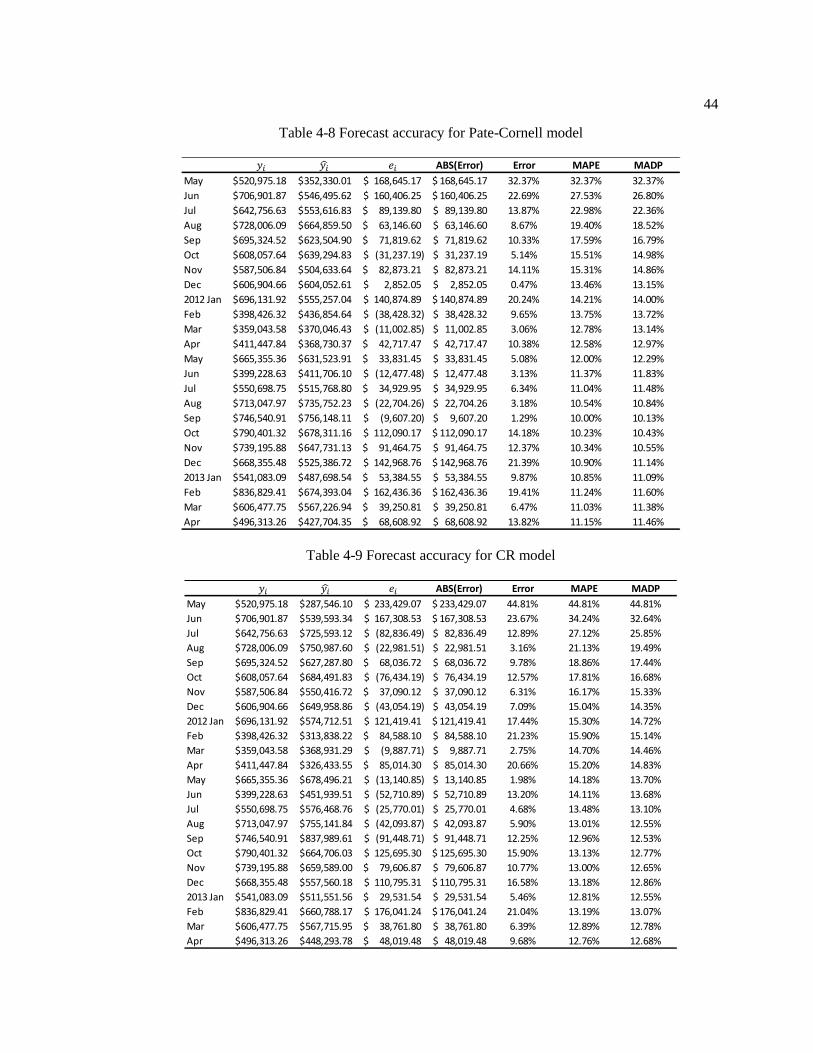
Table 4-8 Forecast accuracy for Pate-Cornell model

Table 4-9 Forecast accuracy for CR model

ABS(Error) Error MAPE MADP

May 520,975.18$ 352,330.01$ 168,645.17$ 168,645.17$ 32.37% 32.37% 32.37%

Jun 706,901.87$ 546,495.62$ 160,406.25$ 160,406.25$ 22.69% 27.53% 26.80%

Jul 642,756.63$ 553,616.83$ 89,139.80$ 89,139.80$ 13.87% 22.98% 22.36%

Aug 728,006.09$ 664,859.50$ 63,146.60$ 63,146.60$ 8.67% 19.40% 18.52%

Sep 695,324.52$ 623,504.90$ 71,819.62$ 71,819.62$ 10.33% 17.59% 16.79%

Oct 608,057.64$ 639,294.83$ (31,237.19)$ 31,237.19$ 5.14% 15.51% 14.98%

Nov 587,506.84$ 504,633.64$ 82,873.21$ 82,873.21$ 14.11% 15.31% 14.86%

Dec 606,904.66$ 604,052.61$ 2,852.05$ 2,852.05$ 0.47% 13.46% 13.15%

2012 Jan 696,131.92$ 555,257.04$ 140,874.89$ 140,874.89$ 20.24% 14.21% 14.00%

Feb 398,426.32$ 436,854.64$ (38,428.32)$ 38,428.32$ 9.65% 13.75% 13.72%

Mar 359,043.58$ 370,046.43$ (11,002.85)$ 11,002.85$ 3.06% 12.78% 13.14%

Apr 411,447.84$ 368,730.37$ 42,717.47$ 42,717.47$ 10.38% 12.58% 12.97%

May 665,355.36$ 631,523.91$ 33,831.45$ 33,831.45$ 5.08% 12.00% 12.29%

Jun 399,228.63$ 411,706.10$ (12,477.48)$ 12,477.48$ 3.13% 11.37% 11.83%

Jul 550,698.75$ 515,768.80$ 34,929.95$ 34,929.95$ 6.34% 11.04% 11.48%

Aug 713,047.97$ 735,752.23$ (22,704.26)$ 22,704.26$ 3.18% 10.54% 10.84%

Sep 746,540.91$ 756,148.11$ (9,607.20)$ 9,607.20$ 1.29% 10.00% 10.13%

Oct 790,401.32$ 678,311.16$ 112,090.17$ 112,090.17$ 14.18% 10.23% 10.43%

Nov 739,195.88$ 647,731.13$ 91,464.75$ 91,464.75$ 12.37% 10.34% 10.55%

Dec 668,355.48$ 525,386.72$ 142,968.76$ 142,968.76$ 21.39% 10.90% 11.14%

2013 Jan 541,083.09$ 487,698.54$ 53,384.55$ 53,384.55$ 9.87% 10.85% 11.09%

Feb 836,829.41$ 674,393.04$ 162,436.36$ 162,436.36$ 19.41% 11.24% 11.60%

Mar 606,477.75$ 567,226.94$ 39,250.81$ 39,250.81$ 6.47% 11.03% 11.38%

Apr 496,313.26$ 427,704.35$ 68,608.92$ 68,608.92$ 13.82% 11.15% 11.46%

𝑖 𝑖 𝑒𝑖

ABS(Error) Error MAPE MADP

May 520,975.18$ 287,546.10$ 233,429.07$ 233,429.07$ 44.81% 44.81% 44.81%

Jun 706,901.87$ 539,593.34$ 167,308.53$ 167,308.53$ 23.67% 34.24% 32.64%

Jul 642,756.63$ 725,593.12$ (82,836.49)$ 82,836.49$ 12.89% 27.12% 25.85%

Aug 728,006.09$ 750,987.60$ (22,981.51)$ 22,981.51$ 3.16% 21.13% 19.49%

Sep 695,324.52$ 627,287.80$ 68,036.72$ 68,036.72$ 9.78% 18.86% 17.44%

Oct 608,057.64$ 684,491.83$ (76,434.19)$ 76,434.19$ 12.57% 17.81% 16.68%

Nov 587,506.84$ 550,416.72$ 37,090.12$ 37,090.12$ 6.31% 16.17% 15.33%

Dec 606,904.66$ 649,958.86$ (43,054.19)$ 43,054.19$ 7.09% 15.04% 14.35%

2012 Jan 696,131.92$ 574,712.51$ 121,419.41$ 121,419.41$ 17.44% 15.30% 14.72%

Feb 398,426.32$ 313,838.22$ 84,588.10$ 84,588.10$ 21.23% 15.90% 15.14%

Mar 359,043.58$ 368,931.29$ (9,887.71)$ 9,887.71$ 2.75% 14.70% 14.46%

Apr 411,447.84$ 326,433.55$ 85,014.30$ 85,014.30$ 20.66% 15.20% 14.83%

May 665,355.36$ 678,496.21$ (13,140.85)$ 13,140.85$ 1.98% 14.18% 13.70%

Jun 399,228.63$ 451,939.51$ (52,710.89)$ 52,710.89$ 13.20% 14.11% 13.68%

Jul 550,698.75$ 576,468.76$ (25,770.01)$ 25,770.01$ 4.68% 13.48% 13.10%

Aug 713,047.97$ 755,141.84$ (42,093.87)$ 42,093.87$ 5.90% 13.01% 12.55%

Sep 746,540.91$ 837,989.61$ (91,448.71)$ 91,448.71$ 12.25% 12.96% 12.53%

Oct 790,401.32$ 664,706.03$ 125,695.30$ 125,695.30$ 15.90% 13.13% 12.77%

Nov 739,195.88$ 659,589.00$ 79,606.87$ 79,606.87$ 10.77% 13.00% 12.65%

Dec 668,355.48$ 557,560.18$ 110,795.31$ 110,795.31$ 16.58% 13.18% 12.86%

2013 Jan 541,083.09$ 511,551.56$ 29,531.54$ 29,531.54$ 5.46% 12.81% 12.55%

Feb 836,829.41$ 660,788.17$ 176,041.24$ 176,041.24$ 21.04% 13.19% 13.07%

Mar 606,477.75$ 567,715.95$ 38,761.80$ 38,761.80$ 6.39% 12.89% 12.78%

Apr 496,313.26$ 448,293.78$ 48,019.48$ 48,019.48$ 9.68% 12.76% 12.68%

𝑖 𝑖 𝑒𝑖

45

Table 4-10 Forecast accuracy for Jeep model

Table 4-11 Forecast accuracy for Combine model

ABS(Error) Error MAPE MADP

May 520,975.18$ 384,028.19$ 136,946.98$ 136,946.98$ 26.29% 26.29% 26.29%

Jun 706,901.87$ 597,120.39$ 109,781.48$ 109,781.48$ 15.53% 20.91% 20.09%

Jul 642,756.63$ 667,701.55$ (24,944.92)$ 24,944.92$ 3.88% 15.23% 14.52%

Aug 728,006.09$ 775,039.65$ (47,033.56)$ 47,033.56$ 6.46% 13.04% 12.26%

Sep 695,324.52$ 663,459.32$ 31,865.20$ 31,865.20$ 4.58% 11.35% 10.64%

Oct 608,057.64$ 647,981.41$ (39,923.77)$ 39,923.77$ 6.57% 10.55% 10.01%

Nov 587,506.84$ 614,627.03$ (27,120.19)$ 27,120.19$ 4.62% 9.70% 9.30%

Dec 606,904.66$ 684,721.35$ (77,816.69)$ 77,816.69$ 12.82% 10.09% 9.72%

2012 Jan 696,131.92$ 623,750.27$ 72,381.65$ 72,381.65$ 10.40% 10.13% 9.80%

Feb 398,426.32$ 460,852.42$ (62,426.10)$ 62,426.10$ 15.67% 10.68% 10.18%

Mar 359,043.58$ 441,744.89$ (82,701.31)$ 82,701.31$ 23.03% 11.80% 10.88%

Apr 411,447.84$ 410,672.29$ 775.56$ 775.56$ 0.19% 10.84% 10.25%

May 665,355.36$ 632,339.31$ 33,016.05$ 33,016.05$ 4.96% 10.38% 9.79%

Jun 399,228.63$ 471,590.36$ (72,361.73)$ 72,361.73$ 18.13% 10.94% 10.21%

Jul 550,698.75$ 569,545.89$ (18,847.14)$ 18,847.14$ 3.42% 10.44% 9.77%

Aug 713,047.97$ 798,504.63$ (85,456.66)$ 85,456.66$ 11.98% 10.53% 9.94%

Sep 746,540.91$ 838,635.81$ (92,094.90)$ 92,094.90$ 12.34% 10.64% 10.12%

Oct 790,401.32$ 810,472.79$ (20,071.47)$ 20,071.47$ 2.54% 10.19% 9.56%

Nov 739,195.88$ 720,592.65$ 18,603.23$ 18,603.23$ 2.52% 9.79% 9.11%

Dec 668,355.48$ 613,403.19$ 54,952.30$ 54,952.30$ 8.22% 9.71% 9.07%

2013 Jan 541,083.09$ 588,486.85$ (47,403.75)$ 47,403.75$ 8.76% 9.66% 9.05%

Feb 836,829.41$ 803,926.30$ 32,903.11$ 32,903.11$ 3.93% 9.40% 8.74%

Mar 606,477.75$ 629,940.16$ (23,462.41)$ 23,462.41$ 3.87% 9.16% 8.53%

Apr 496,313.26$ 536,253.16$ (39,939.90)$ 39,939.90$ 8.05% 9.11% 8.51%

𝑖 𝑖 𝑒𝑖

ABS(Error) Error MAPE MADP

May 520,975.18$ $392,438.68 128,536.50$ 128,536.50$ 24.67% 24.67% 24.67%

Jun 706,901.87$ $603,812.30 103,089.57$ 103,089.57$ 14.58% 19.63% 18.86%

Jul 642,756.63$ $672,318.35 (29,561.73)$ 29,561.73$ 4.60% 14.62% 13.96%

Aug 728,006.09$ $782,129.83 (54,123.74)$ 54,123.74$ 7.43% 12.82% 12.13%

Sep 695,324.52$ $677,349.31 17,975.21$ 17,975.21$ 2.59% 10.77% 10.12%

Oct 608,057.64$ $662,274.82 (54,217.18)$ 54,217.18$ 8.92% 10.47% 9.93%

Nov 587,506.84$ $621,473.16 (33,966.32)$ 33,966.32$ 5.78% 9.80% 9.39%

Dec 606,904.66$ $691,719.21 (84,814.55)$ 84,814.55$ 13.97% 10.32% 9.93%

2012 Jan 696,131.92$ $623,318.95 72,812.97$ 72,812.97$ 10.46% 10.33% 10.00%

Feb 398,426.32$ $461,083.58 (62,657.26)$ 62,657.26$ 15.73% 10.87% 10.37%

Mar 359,043.58$ $404,565.04 (45,521.46)$ 45,521.46$ 12.68% 11.04% 10.49%

Apr 411,447.84$ $408,577.57 2,870.27$ 2,870.27$ 0.70% 10.18% 9.91%

May 665,355.36$ $686,168.96 (20,813.60)$ 20,813.60$ 3.13% 9.63% 9.32%

Jun 399,228.63$ $474,487.31 (75,258.69)$ 75,258.69$ 18.85% 10.29% 9.80%

Jul 550,698.75$ $566,805.72 (16,106.97)$ 16,106.97$ 2.92% 9.80% 9.35%

Aug 713,047.97$ $800,916.23 (87,868.26)$ 87,868.26$ 12.32% 9.96% 9.58%

Sep 746,540.91$ $837,866.72 (91,325.81)$ 91,325.81$ 12.23% 10.09% 9.78%

Oct 790,401.32$ $813,899.51 (23,498.19)$ 23,498.19$ 2.97% 9.70% 9.28%

Nov 739,195.88$ $722,704.04 16,491.84$ 16,491.84$ 2.23% 9.30% 8.83%

Dec 668,355.48$ $608,393.13 59,962.35$ 59,962.35$ 8.97% 9.29% 8.84%

2013 Jan 541,083.09$ $563,039.93 (21,956.84)$ 21,956.84$ 4.06% 9.04% 8.64%

Feb 836,829.41$ $785,105.99 51,723.42$ 51,723.42$ 6.18% 8.91% 8.49%

Mar 606,477.75$ $624,323.42 (17,845.67)$ 17,845.67$ 2.94% 8.65% 8.25%

Apr 496,313.26$ $536,191.16 (39,877.90)$ 39,877.90$ 8.03% 8.62% 8.24%

𝑖 𝑖 𝑒𝑖

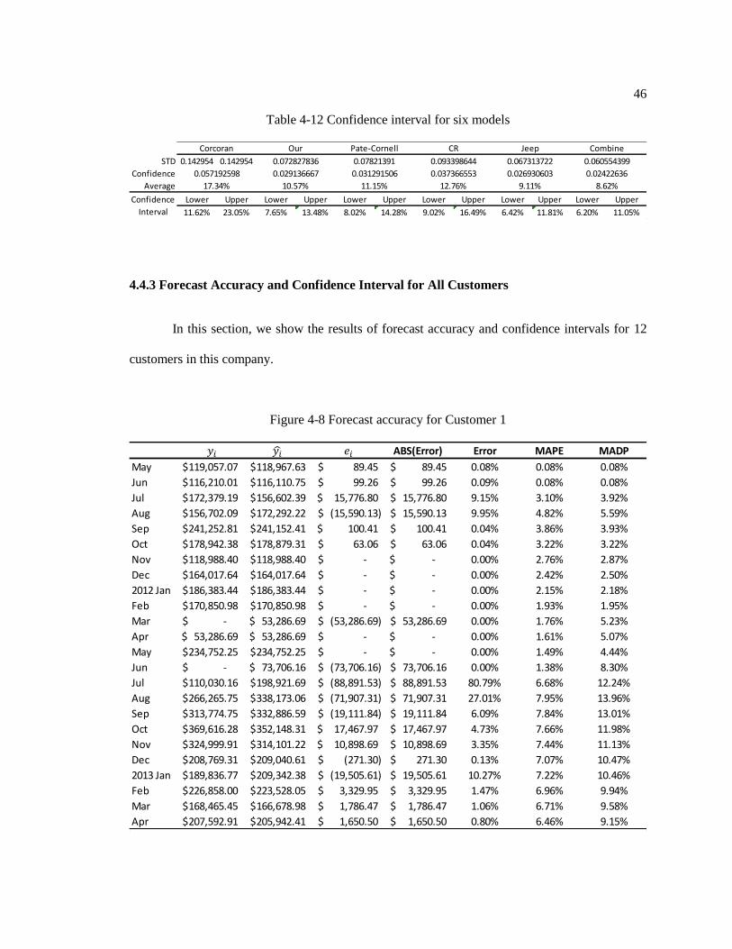
46

Table 4-12 Confidence interval for six models

4.4.3 Forecast Accuracy and Confidence Interval for All Customers

In this section, we show the results of forecast accuracy and confidence intervals for 12

customers in this company.

Figure 4-8 Forecast accuracy for Customer 1

STD 0.142954 0.142954

Confidence

Average

Lower Upper Lower Upper Lower Upper Lower Upper Lower Upper Lower Upper

11.62% 23.05% 7.65% 13.48% 8.02% 14.28% 9.02% 16.49% 6.42% 11.81% 6.20% 11.05%

0.060554399

Corcoran Our Pate-Cornell CR Jeep Combine

0.072827836 0.07821391 0.093398644 0.067313722

9.11% 8.62%

0.057192598 0.029136667 0.031291506 0.037366553 0.026930603 0.02422636

Confidence

Interval

17.34% 10.57% 11.15% 12.76%

ABS(Error) Error MAPE MADP

May 119,057.07$ 118,967.63$ 89.45$ 89.45$ 0.08% 0.08% 0.08%

Jun 116,210.01$ 116,110.75$ 99.26$ 99.26$ 0.09% 0.08% 0.08%

Jul 172,379.19$ 156,602.39$ 15,776.80$ 15,776.80$ 9.15% 3.10% 3.92%

Aug 156,702.09$ 172,292.22$ (15,590.13)$ 15,590.13$ 9.95% 4.82% 5.59%

Sep 241,252.81$ 241,152.41$ 100.41$ 100.41$ 0.04% 3.86% 3.93%

Oct 178,942.38$ 178,879.31$ 63.06$ 63.06$ 0.04% 3.22% 3.22%

Nov 118,988.40$ 118,988.40$ -$ -$ 0.00% 2.76% 2.87%

Dec 164,017.64$ 164,017.64$ -$ -$ 0.00% 2.42% 2.50%

2012 Jan 186,383.44$ 186,383.44$ -$ -$ 0.00% 2.15% 2.18%

Feb 170,850.98$ 170,850.98$ -$ -$ 0.00% 1.93% 1.95%

Mar -$ 53,286.69$ (53,286.69)$ 53,286.69$ 0.00% 1.76% 5.23%

Apr 53,286.69$ 53,286.69$ -$ -$ 0.00% 1.61% 5.07%

May 234,752.25$ 234,752.25$ -$ -$ 0.00% 1.49% 4.44%

Jun -$ 73,706.16$ (73,706.16)$ 73,706.16$ 0.00% 1.38% 8.30%

Jul 110,030.16$ 198,921.69$ (88,891.53)$ 88,891.53$ 80.79% 6.68% 12.24%

Aug 266,265.75$ 338,173.06$ (71,907.31)$ 71,907.31$ 27.01% 7.95% 13.96%

Sep 313,774.75$ 332,886.59$ (19,111.84)$ 19,111.84$ 6.09% 7.84% 13.01%

Oct 369,616.28$ 352,148.31$ 17,467.97$ 17,467.97$ 4.73% 7.66% 11.98%

Nov 324,999.91$ 314,101.22$ 10,898.69$ 10,898.69$ 3.35% 7.44% 11.13%

Dec 208,769.31$ 209,040.61$ (271.30)$ 271.30$ 0.13% 7.07% 10.47%

2013 Jan 189,836.77$ 209,342.38$ (19,505.61)$ 19,505.61$ 10.27% 7.22% 10.46%

Feb 226,858.00$ 223,528.05$ 3,329.95$ 3,329.95$ 1.47% 6.96% 9.94%

Mar 168,465.45$ 166,678.98$ 1,786.47$ 1,786.47$ 1.06% 6.71% 9.58%

Apr 207,592.91$ 205,942.41$ 1,650.50$ 1,650.50$ 0.80% 6.46% 9.15%

𝑖 𝑖 𝑒𝑖

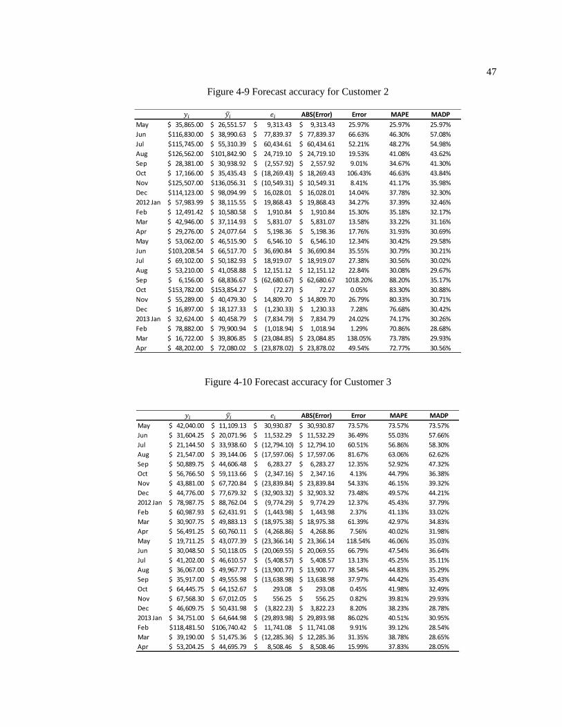
47

Figure 4-9 Forecast accuracy for Customer 2

Figure 4-10 Forecast accuracy for Customer 3

ABS(Error) Error MAPE MADP

May 35,865.00$ 26,551.57$ 9,313.43$ 9,313.43$ 25.97% 25.97% 25.97%

Jun 116,830.00$ 38,990.63$ 77,839.37$ 77,839.37$ 66.63% 46.30% 57.08%

Jul 115,745.00$ 55,310.39$ 60,434.61$ 60,434.61$ 52.21% 48.27% 54.98%

Aug 126,562.00$ 101,842.90$ 24,719.10$ 24,719.10$ 19.53% 41.08% 43.62%

Sep 28,381.00$ 30,938.92$ (2,557.92)$ 2,557.92$ 9.01% 34.67% 41.30%

Oct 17,166.00$ 35,435.43$ (18,269.43)$ 18,269.43$ 106.43% 46.63% 43.84%

Nov 125,507.00$ 136,056.31$ (10,549.31)$ 10,549.31$ 8.41% 41.17% 35.98%

Dec 114,123.00$ 98,094.99$ 16,028.01$ 16,028.01$ 14.04% 37.78% 32.30%

2012 Jan 57,983.99$ 38,115.55$ 19,868.43$ 19,868.43$ 34.27% 37.39% 32.46%

Feb 12,491.42$ 10,580.58$ 1,910.84$ 1,910.84$ 15.30% 35.18% 32.17%

Mar 42,946.00$ 37,114.93$ 5,831.07$ 5,831.07$ 13.58% 33.22% 31.16%

Apr 29,276.00$ 24,077.64$ 5,198.36$ 5,198.36$ 17.76% 31.93% 30.69%

May 53,062.00$ 46,515.90$ 6,546.10$ 6,546.10$ 12.34% 30.42% 29.58%

Jun 103,208.54$ 66,517.70$ 36,690.84$ 36,690.84$ 35.55% 30.79% 30.21%

Jul 69,102.00$ 50,182.93$ 18,919.07$ 18,919.07$ 27.38% 30.56% 30.02%

Aug 53,210.00$ 41,058.88$ 12,151.12$ 12,151.12$ 22.84% 30.08% 29.67%

Sep 6,156.00$ 68,836.67$ (62,680.67)$ 62,680.67$ 1018.20% 88.20% 35.17%

Oct 153,782.00$ 153,854.27$ (72.27)$ 72.27$ 0.05% 83.30% 30.88%

Nov 55,289.00$ 40,479.30$ 14,809.70$ 14,809.70$ 26.79% 80.33% 30.71%

Dec 16,897.00$ 18,127.33$ (1,230.33)$ 1,230.33$ 7.28% 76.68% 30.42%

2013 Jan 32,624.00$ 40,458.79$ (7,834.79)$ 7,834.79$ 24.02% 74.17% 30.26%

Feb 78,882.00$ 79,900.94$ (1,018.94)$ 1,018.94$ 1.29% 70.86% 28.68%

Mar 16,722.00$ 39,806.85$ (23,084.85)$ 23,084.85$ 138.05% 73.78% 29.93%

Apr 48,202.00$ 72,080.02$ (23,878.02)$ 23,878.02$ 49.54% 72.77% 30.56%

𝑖 𝑖 𝑒𝑖

ABS(Error) Error MAPE MADP

May 42,040.00$ 11,109.13$ 30,930.87$ 30,930.87$ 73.57% 73.57% 73.57%

Jun 31,604.25$ 20,071.96$ 11,532.29$ 11,532.29$ 36.49% 55.03% 57.66%

Jul 21,144.50$ 33,938.60$ (12,794.10)$ 12,794.10$ 60.51% 56.86% 58.30%

Aug 21,547.00$ 39,144.06$ (17,597.06)$ 17,597.06$ 81.67% 63.06% 62.62%

Sep 50,889.75$ 44,606.48$ 6,283.27$ 6,283.27$ 12.35% 52.92% 47.32%

Oct 56,766.50$ 59,113.66$ (2,347.16)$ 2,347.16$ 4.13% 44.79% 36.38%

Nov 43,881.00$ 67,720.84$ (23,839.84)$ 23,839.84$ 54.33% 46.15% 39.32%

Dec 44,776.00$ 77,679.32$ (32,903.32)$ 32,903.32$ 73.48% 49.57% 44.21%

2012 Jan 78,987.75$ 88,762.04$ (9,774.29)$ 9,774.29$ 12.37% 45.43% 37.79%

Feb 60,987.93$ 62,431.91$ (1,443.98)$ 1,443.98$ 2.37% 41.13% 33.02%

Mar 30,907.75$ 49,883.13$ (18,975.38)$ 18,975.38$ 61.39% 42.97% 34.83%

Apr 56,491.25$ 60,760.11$ (4,268.86)$ 4,268.86$ 7.56% 40.02% 31.98%

May 19,711.25$ 43,077.39$ (23,366.14)$ 23,366.14$ 118.54% 46.06% 35.03%

Jun 30,048.50$ 50,118.05$ (20,069.55)$ 20,069.55$ 66.79% 47.54% 36.64%

Jul 41,202.00$ 46,610.57$ (5,408.57)$ 5,408.57$ 13.13% 45.25% 35.11%

Aug 36,067.00$ 49,967.77$ (13,900.77)$ 13,900.77$ 38.54% 44.83% 35.29%

Sep 35,917.00$ 49,555.98$ (13,638.98)$ 13,638.98$ 37.97% 44.42% 35.43%

Oct 64,445.75$ 64,152.67$ 293.08$ 293.08$ 0.45% 41.98% 32.49%

Nov 67,568.30$ 67,012.05$ 556.25$ 556.25$ 0.82% 39.81% 29.93%

Dec 46,609.75$ 50,431.98$ (3,822.23)$ 3,822.23$ 8.20% 38.23% 28.78%

2013 Jan 34,751.00$ 64,644.98$ (29,893.98)$ 29,893.98$ 86.02% 40.51% 30.95%

Feb 118,481.50$ 106,740.42$ 11,741.08$ 11,741.08$ 9.91% 39.12% 28.54%

Mar 39,190.00$ 51,475.36$ (12,285.36)$ 12,285.36$ 31.35% 38.78% 28.65%

Apr 53,204.25$ 44,695.79$ 8,508.46$ 8,508.46$ 15.99% 37.83% 28.05%

𝑖 𝑖 𝑒𝑖

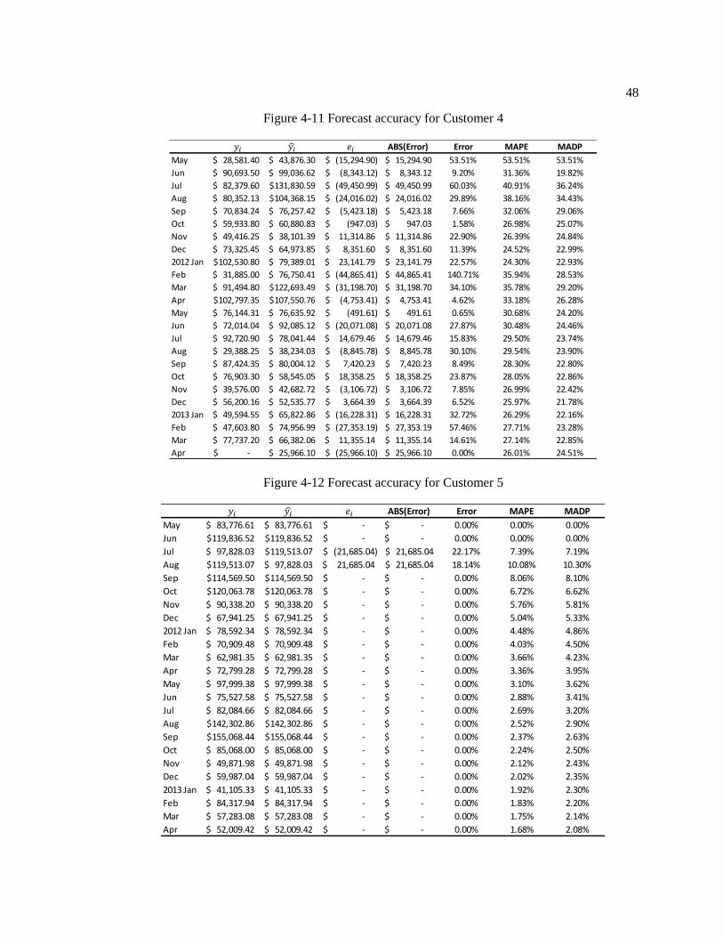
48

Figure 4-11 Forecast accuracy for Customer 4

Figure 4-12 Forecast accuracy for Customer 5

ABS(Error) Error MAPE MADP

May 28,581.40$ 43,876.30$ (15,294.90)$ 15,294.90$ 53.51% 53.51% 53.51%

Jun 90,693.50$ 99,036.62$ (8,343.12)$ 8,343.12$ 9.20% 31.36% 19.82%

Jul 82,379.60$ 131,830.59$ (49,450.99)$ 49,450.99$ 60.03% 40.91% 36.24%

Aug 80,352.13$ 104,368.15$ (24,016.02)$ 24,016.02$ 29.89% 38.16% 34.43%

Sep 70,834.24$ 76,257.42$ (5,423.18)$ 5,423.18$ 7.66% 32.06% 29.06%

Oct 59,933.80$ 60,880.83$ (947.03)$ 947.03$ 1.58% 26.98% 25.07%

Nov 49,416.25$ 38,101.39$ 11,314.86$ 11,314.86$ 22.90% 26.39% 24.84%

Dec 73,325.45$ 64,973.85$ 8,351.60$ 8,351.60$ 11.39% 24.52% 22.99%

2012 Jan 102,530.80$ 79,389.01$ 23,141.79$ 23,141.79$ 22.57% 24.30% 22.93%

Feb 31,885.00$ 76,750.41$ (44,865.41)$ 44,865.41$ 140.71% 35.94% 28.53%

Mar 91,494.80$ 122,693.49$ (31,198.70)$ 31,198.70$ 34.10% 35.78% 29.20%

Apr 102,797.35$ 107,550.76$ (4,753.41)$ 4,753.41$ 4.62% 33.18% 26.28%

May 76,144.31$ 76,635.92$ (491.61)$ 491.61$ 0.65% 30.68% 24.20%

Jun 72,014.04$ 92,085.12$ (20,071.08)$ 20,071.08$ 27.87% 30.48% 24.46%

Jul 92,720.90$ 78,041.44$ 14,679.46$ 14,679.46$ 15.83% 29.50% 23.74%

Aug 29,388.25$ 38,234.03$ (8,845.78)$ 8,845.78$ 30.10% 29.54% 23.90%

Sep 87,424.35$ 80,004.12$ 7,420.23$ 7,420.23$ 8.49% 28.30% 22.80%

Oct 76,903.30$ 58,545.05$ 18,358.25$ 18,358.25$ 23.87% 28.05% 22.86%

Nov 39,576.00$ 42,682.72$ (3,106.72)$ 3,106.72$ 7.85% 26.99% 22.42%

Dec 56,200.16$ 52,535.77$ 3,664.39$ 3,664.39$ 6.52% 25.97% 21.78%

2013 Jan 49,594.55$ 65,822.86$ (16,228.31)$ 16,228.31$ 32.72% 26.29% 22.16%

Feb 47,603.80$ 74,956.99$ (27,353.19)$ 27,353.19$ 57.46% 27.71% 23.28%

Mar 77,737.20$ 66,382.06$ 11,355.14$ 11,355.14$ 14.61% 27.14% 22.85%

Apr -$ 25,966.10$ (25,966.10)$ 25,966.10$ 0.00% 26.01% 24.51%

𝑖 𝑖 𝑒𝑖

ABS(Error) Error MAPE MADP

May 83,776.61$ 83,776.61$ -$ -$ 0.00% 0.00% 0.00%

Jun 119,836.52$ 119,836.52$ -$ -$ 0.00% 0.00% 0.00%

Jul 97,828.03$ 119,513.07$ (21,685.04)$ 21,685.04$ 22.17% 7.39% 7.19%

Aug 119,513.07$ 97,828.03$ 21,685.04$ 21,685.04$ 18.14% 10.08% 10.30%

Sep 114,569.50$ 114,569.50$ -$ -$ 0.00% 8.06% 8.10%

Oct 120,063.78$ 120,063.78$ -$ -$ 0.00% 6.72% 6.62%

Nov 90,338.20$ 90,338.20$ -$ -$ 0.00% 5.76% 5.81%

Dec 67,941.25$ 67,941.25$ -$ -$ 0.00% 5.04% 5.33%

2012 Jan 78,592.34$ 78,592.34$ -$ -$ 0.00% 4.48% 4.86%

Feb 70,909.48$ 70,909.48$ -$ -$ 0.00% 4.03% 4.50%

Mar 62,981.35$ 62,981.35$ -$ -$ 0.00% 3.66% 4.23%

Apr 72,799.28$ 72,799.28$ -$ -$ 0.00% 3.36% 3.95%

May 97,999.38$ 97,999.38$ -$ -$ 0.00% 3.10% 3.62%

Jun 75,527.58$ 75,527.58$ -$ -$ 0.00% 2.88% 3.41%

Jul 82,084.66$ 82,084.66$ -$ -$ 0.00% 2.69% 3.20%

Aug 142,302.86$ 142,302.86$ -$ -$ 0.00% 2.52% 2.90%

Sep 155,068.44$ 155,068.44$ -$ -$ 0.00% 2.37% 2.63%

Oct 85,068.00$ 85,068.00$ -$ -$ 0.00% 2.24% 2.50%

Nov 49,871.98$ 49,871.98$ -$ -$ 0.00% 2.12% 2.43%

Dec 59,987.04$ 59,987.04$ -$ -$ 0.00% 2.02% 2.35%

2013 Jan 41,105.33$ 41,105.33$ -$ -$ 0.00% 1.92% 2.30%

Feb 84,317.94$ 84,317.94$ -$ -$ 0.00% 1.83% 2.20%

Mar 57,283.08$ 57,283.08$ -$ -$ 0.00% 1.75% 2.14%

Apr 52,009.42$ 52,009.42$ -$ -$ 0.00% 1.68% 2.08%

𝑖 𝑖 𝑒𝑖

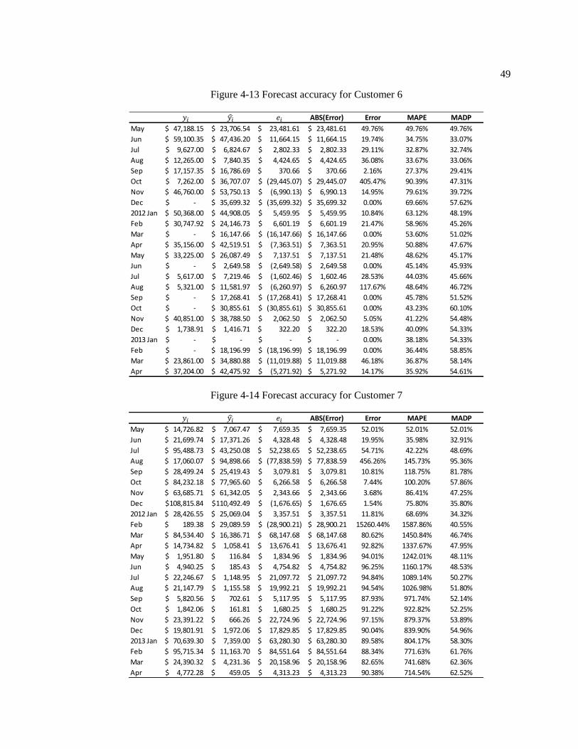
49

Figure 4-13 Forecast accuracy for Customer 6

Figure 4-14 Forecast accuracy for Customer 7

ABS(Error) Error MAPE MADP

May 47,188.15$ 23,706.54$ 23,481.61$ 23,481.61$ 49.76% 49.76% 49.76%

Jun 59,100.35$ 47,436.20$ 11,664.15$ 11,664.15$ 19.74% 34.75% 33.07%

Jul 9,627.00$ 6,824.67$ 2,802.33$ 2,802.33$ 29.11% 32.87% 32.74%

Aug 12,265.00$ 7,840.35$ 4,424.65$ 4,424.65$ 36.08% 33.67% 33.06%

Sep 17,157.35$ 16,786.69$ 370.66$ 370.66$ 2.16% 27.37% 29.41%

Oct 7,262.00$ 36,707.07$ (29,445.07)$ 29,445.07$ 405.47% 90.39% 47.31%

Nov 46,760.00$ 53,750.13$ (6,990.13)$ 6,990.13$ 14.95% 79.61% 39.72%

Dec -$ 35,699.32$ (35,699.32)$ 35,699.32$ 0.00% 69.66% 57.62%

2012 Jan 50,368.00$ 44,908.05$ 5,459.95$ 5,459.95$ 10.84% 63.12% 48.19%

Feb 30,747.92$ 24,146.73$ 6,601.19$ 6,601.19$ 21.47% 58.96% 45.26%

Mar -$ 16,147.66$ (16,147.66)$ 16,147.66$ 0.00% 53.60% 51.02%

Apr 35,156.00$ 42,519.51$ (7,363.51)$ 7,363.51$ 20.95% 50.88% 47.67%

May 33,225.00$ 26,087.49$ 7,137.51$ 7,137.51$ 21.48% 48.62% 45.17%

Jun -$ 2,649.58$ (2,649.58)$ 2,649.58$ 0.00% 45.14% 45.93%

Jul 5,617.00$ 7,219.46$ (1,602.46)$ 1,602.46$ 28.53% 44.03% 45.66%

Aug 5,321.00$ 11,581.97$ (6,260.97)$ 6,260.97$ 117.67% 48.64% 46.72%

Sep -$ 17,268.41$ (17,268.41)$ 17,268.41$ 0.00% 45.78% 51.52%

Oct -$ 30,855.61$ (30,855.61)$ 30,855.61$ 0.00% 43.23% 60.10%

Nov 40,851.00$ 38,788.50$ 2,062.50$ 2,062.50$ 5.05% 41.22% 54.48%

Dec 1,738.91$ 1,416.71$ 322.20$ 322.20$ 18.53% 40.09% 54.33%

2013 Jan -$ -$ -$ -$ 0.00% 38.18% 54.33%

Feb -$ 18,196.99$ (18,196.99)$ 18,196.99$ 0.00% 36.44% 58.85%

Mar 23,861.00$ 34,880.88$ (11,019.88)$ 11,019.88$ 46.18% 36.87% 58.14%

Apr 37,204.00$ 42,475.92$ (5,271.92)$ 5,271.92$ 14.17% 35.92% 54.61%

𝑖 𝑖 𝑒𝑖

ABS(Error) Error MAPE MADP

May 14,726.82$ 7,067.47$ 7,659.35$ 7,659.35$ 52.01% 52.01% 52.01%

Jun 21,699.74$ 17,371.26$ 4,328.48$ 4,328.48$ 19.95% 35.98% 32.91%

Jul 95,488.73$ 43,250.08$ 52,238.65$ 52,238.65$ 54.71% 42.22% 48.69%

Aug 17,060.07$ 94,898.66$ (77,838.59)$ 77,838.59$ 456.26% 145.73% 95.36%

Sep 28,499.24$ 25,419.43$ 3,079.81$ 3,079.81$ 10.81% 118.75% 81.78%

Oct 84,232.18$ 77,965.60$ 6,266.58$ 6,266.58$ 7.44% 100.20% 57.86%

Nov 63,685.71$ 61,342.05$ 2,343.66$ 2,343.66$ 3.68% 86.41% 47.25%

Dec 108,815.84$ 110,492.49$ (1,676.65)$ 1,676.65$ 1.54% 75.80% 35.80%

2012 Jan 28,426.55$ 25,069.04$ 3,357.51$ 3,357.51$ 11.81% 68.69% 34.32%

Feb 189.38$ 29,089.59$ (28,900.21)$ 28,900.21$ 15260.44% 1587.86% 40.55%

Mar 84,534.40$ 16,386.71$ 68,147.68$ 68,147.68$ 80.62% 1450.84% 46.74%

Apr 14,734.82$ 1,058.41$ 13,676.41$ 13,676.41$ 92.82% 1337.67% 47.95%

May 1,951.80$ 116.84$ 1,834.96$ 1,834.96$ 94.01% 1242.01% 48.11%

Jun 4,940.25$ 185.43$ 4,754.82$ 4,754.82$ 96.25% 1160.17% 48.53%

Jul 22,246.67$ 1,148.95$ 21,097.72$ 21,097.72$ 94.84% 1089.14% 50.27%

Aug 21,147.79$ 1,155.58$ 19,992.21$ 19,992.21$ 94.54% 1026.98% 51.80%

Sep 5,820.56$ 702.61$ 5,117.95$ 5,117.95$ 87.93% 971.74% 52.14%

Oct 1,842.06$ 161.81$ 1,680.25$ 1,680.25$ 91.22% 922.82% 52.25%

Nov 23,391.22$ 666.26$ 22,724.96$ 22,724.96$ 97.15% 879.37% 53.89%

Dec 19,801.91$ 1,972.06$ 17,829.85$ 17,829.85$ 90.04% 839.90% 54.96%

2013 Jan 70,639.30$ 7,359.00$ 63,280.30$ 63,280.30$ 89.58% 804.17% 58.30%

Feb 95,715.34$ 11,163.70$ 84,551.64$ 84,551.64$ 88.34% 771.63% 61.76%

Mar 24,390.32$ 4,231.36$ 20,158.96$ 20,158.96$ 82.65% 741.68% 62.36%

Apr 4,772.28$ 459.05$ 4,313.23$ 4,313.23$ 90.38% 714.54% 62.52%

𝑖 𝑖 𝑒𝑖

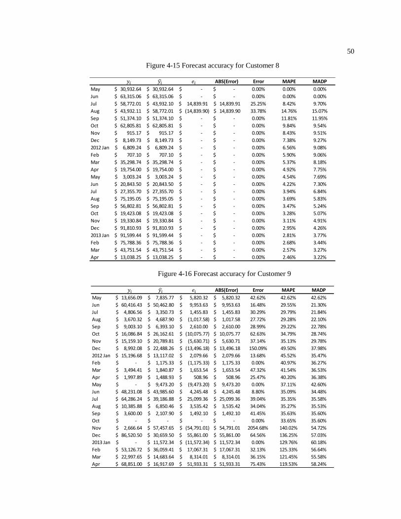
50

Figure 4-15 Forecast accuracy for Customer 8

Figure 4-16 Forecast accuracy for Customer 9

ABS(Error) Error MAPE MADP

May 30,932.64$ 30,932.64$ -$ -$ 0.00% 0.00% 0.00%

Jun 63,315.06$ 63,315.06$ -$ -$ 0.00% 0.00% 0.00%

Jul 58,772.01$ 43,932.10$ 14,839.91$ 14,839.91$ 25.25% 8.42% 9.70%

Aug 43,932.11$ 58,772.01$ (14,839.90)$ 14,839.90$ 33.78% 14.76% 15.07%

Sep 51,374.10$ 51,374.10$ -$ -$ 0.00% 11.81% 11.95%

Oct 62,805.81$ 62,805.81$ -$ -$ 0.00% 9.84% 9.54%

Nov 915.17$ 915.17$ -$ -$ 0.00% 8.43% 9.51%

Dec 8,149.73$ 8,149.73$ -$ -$ 0.00% 7.38% 9.27%

2012 Jan 6,809.24$ 6,809.24$ -$ -$ 0.00% 6.56% 9.08%

Feb 707.10$ 707.10$ -$ -$ 0.00% 5.90% 9.06%

Mar 35,298.74$ 35,298.74$ -$ -$ 0.00% 5.37% 8.18%

Apr 19,754.00$ 19,754.00$ -$ -$ 0.00% 4.92% 7.75%

May 3,003.24$ 3,003.24$ -$ -$ 0.00% 4.54% 7.69%

Jun 20,843.50$ 20,843.50$ -$ -$ 0.00% 4.22% 7.30%

Jul 27,355.70$ 27,355.70$ -$ -$ 0.00% 3.94% 6.84%

Aug 75,195.05$ 75,195.05$ -$ -$ 0.00% 3.69% 5.83%

Sep 56,802.81$ 56,802.81$ -$ -$ 0.00% 3.47% 5.24%

Oct 19,423.08$ 19,423.08$ -$ -$ 0.00% 3.28% 5.07%

Nov 19,330.84$ 19,330.84$ -$ -$ 0.00% 3.11% 4.91%

Dec 91,810.93$ 91,810.93$ -$ -$ 0.00% 2.95% 4.26%

2013 Jan 91,599.44$ 91,599.44$ -$ -$ 0.00% 2.81% 3.77%

Feb 75,788.36$ 75,788.36$ -$ -$ 0.00% 2.68% 3.44%

Mar 43,751.54$ 43,751.54$ -$ -$ 0.00% 2.57% 3.27%

Apr 13,038.25$ 13,038.25$ -$ -$ 0.00% 2.46% 3.22%

𝑖 𝑖 𝑒𝑖

ABS(Error) Error MAPE MADP

May 13,656.09$ 7,835.77$ 5,820.32$ 5,820.32$ 42.62% 42.62% 42.62%

Jun 60,416.43$ 50,462.80$ 9,953.63$ 9,953.63$ 16.48% 29.55% 21.30%

Jul 4,806.56$ 3,350.73$ 1,455.83$ 1,455.83$ 30.29% 29.79% 21.84%

Aug 3,670.32$ 4,687.90$ (1,017.58)$ 1,017.58$ 27.72% 29.28% 22.10%

Sep 9,003.10$ 6,393.10$ 2,610.00$ 2,610.00$ 28.99% 29.22% 22.78%

Oct 16,086.84$ 26,162.61$ (10,075.77)$ 10,075.77$ 62.63% 34.79% 28.74%

Nov 15,159.10$ 20,789.81$ (5,630.71)$ 5,630.71$ 37.14% 35.13% 29.78%

Dec 8,992.08$ 22,488.26$ (13,496.18)$ 13,496.18$ 150.09% 49.50% 37.98%

2012 Jan 15,196.68$ 13,117.02$ 2,079.66$ 2,079.66$ 13.68% 45.52% 35.47%

Feb -$ 1,175.33$ (1,175.33)$ 1,175.33$ 0.00% 40.97% 36.27%

Mar 3,494.41$ 1,840.87$ 1,653.54$ 1,653.54$ 47.32% 41.54% 36.53%

Apr 1,997.89$ 1,488.93$ 508.96$ 508.96$ 25.47% 40.20% 36.38%

May -$ 9,473.20$ (9,473.20)$ 9,473.20$ 0.00% 37.11% 42.60%

Jun 48,231.08$ 43,985.60$ 4,245.48$ 4,245.48$ 8.80% 35.09% 34.48%

Jul 64,286.24$ 39,186.88$ 25,099.36$ 25,099.36$ 39.04% 35.35% 35.58%

Aug 10,385.88$ 6,850.46$ 3,535.42$ 3,535.42$ 34.04% 35.27% 35.53%

Sep 3,600.00$ 2,107.90$ 1,492.10$ 1,492.10$ 41.45% 35.63% 35.60%

Oct -$ -$ -$ -$ 0.00% 33.65% 35.60%

Nov 2,666.64$ 57,457.65$ (54,791.01)$ 54,791.01$ 2054.68% 140.02% 54.72%

Dec 86,520.50$ 30,659.50$ 55,861.00$ 55,861.00$ 64.56% 136.25% 57.03%

2013 Jan -$ 11,572.34$ (11,572.34)$ 11,572.34$ 0.00% 129.76% 60.18%

Feb 53,126.72$ 36,059.41$ 17,067.31$ 17,067.31$ 32.13% 125.33% 56.64%

Mar 22,997.65$ 14,683.64$ 8,314.01$ 8,314.01$ 36.15% 121.45% 55.58%

Apr 68,851.00$ 16,917.69$ 51,933.31$ 51,933.31$ 75.43% 119.53% 58.24%

𝑖 𝑖 𝑒𝑖

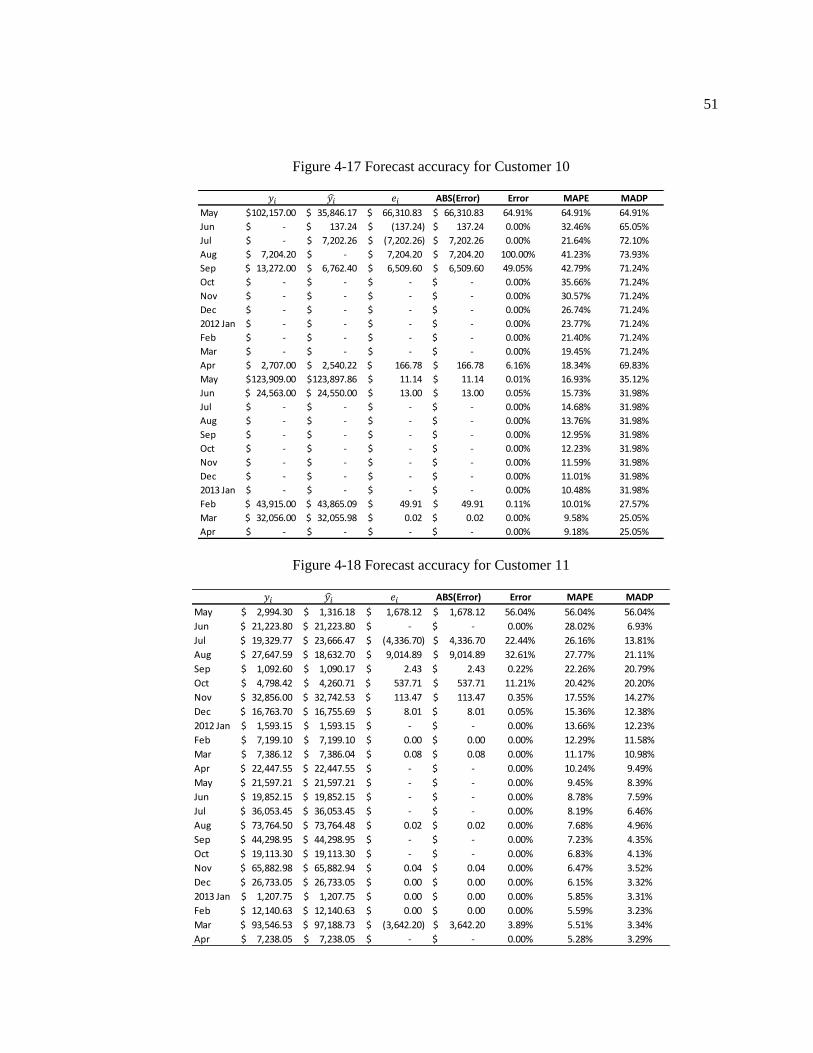
51

Figure 4-17 Forecast accuracy for Customer 10

Figure 4-18 Forecast accuracy for Customer 11

ABS(Error) Error MAPE MADP

May 102,157.00$ 35,846.17$ 66,310.83$ 66,310.83$ 64.91% 64.91% 64.91%

Jun -$ 137.24$ (137.24)$ 137.24$ 0.00% 32.46% 65.05%

Jul -$ 7,202.26$ (7,202.26)$ 7,202.26$ 0.00% 21.64% 72.10%

Aug 7,204.20$ -$ 7,204.20$ 7,204.20$ 100.00% 41.23% 73.93%

Sep 13,272.00$ 6,762.40$ 6,509.60$ 6,509.60$ 49.05% 42.79% 71.24%

Oct -$ -$ -$ -$ 0.00% 35.66% 71.24%

Nov -$ -$ -$ -$ 0.00% 30.57% 71.24%

Dec -$ -$ -$ -$ 0.00% 26.74% 71.24%

2012 Jan -$ -$ -$ -$ 0.00% 23.77% 71.24%

Feb -$ -$ -$ -$ 0.00% 21.40% 71.24%

Mar -$ -$ -$ -$ 0.00% 19.45% 71.24%

Apr 2,707.00$ 2,540.22$ 166.78$ 166.78$ 6.16% 18.34% 69.83%

May 123,909.00$ 123,897.86$ 11.14$ 11.14$ 0.01% 16.93% 35.12%

Jun 24,563.00$ 24,550.00$ 13.00$ 13.00$ 0.05% 15.73% 31.98%

Jul -$ -$ -$ -$ 0.00% 14.68% 31.98%

Aug -$ -$ -$ -$ 0.00% 13.76% 31.98%

Sep -$ -$ -$ -$ 0.00% 12.95% 31.98%

Oct -$ -$ -$ -$ 0.00% 12.23% 31.98%

Nov -$ -$ -$ -$ 0.00% 11.59% 31.98%

Dec -$ -$ -$ -$ 0.00% 11.01% 31.98%

2013 Jan -$ -$ -$ -$ 0.00% 10.48% 31.98%

Feb 43,915.00$ 43,865.09$ 49.91$ 49.91$ 0.11% 10.01% 27.57%

Mar 32,056.00$ 32,055.98$ 0.02$ 0.02$ 0.00% 9.58% 25.05%

Apr -$ -$ -$ -$ 0.00% 9.18% 25.05%

𝑖 𝑖 𝑒𝑖

ABS(Error) Error MAPE MADP

May 2,994.30$ 1,316.18$ 1,678.12$ 1,678.12$ 56.04% 56.04% 56.04%

Jun 21,223.80$ 21,223.80$ -$ -$ 0.00% 28.02% 6.93%

Jul 19,329.77$ 23,666.47$ (4,336.70)$ 4,336.70$ 22.44% 26.16% 13.81%

Aug 27,647.59$ 18,632.70$ 9,014.89$ 9,014.89$ 32.61% 27.77% 21.11%

Sep 1,092.60$ 1,090.17$ 2.43$ 2.43$ 0.22% 22.26% 20.79%

Oct 4,798.42$ 4,260.71$ 537.71$ 537.71$ 11.21% 20.42% 20.20%

Nov 32,856.00$ 32,742.53$ 113.47$ 113.47$ 0.35% 17.55% 14.27%

Dec 16,763.70$ 16,755.69$ 8.01$ 8.01$ 0.05% 15.36% 12.38%

2012 Jan 1,593.15$ 1,593.15$ -$ -$ 0.00% 13.66% 12.23%

Feb 7,199.10$ 7,199.10$ 0.00$ 0.00$ 0.00% 12.29% 11.58%

Mar 7,386.12$ 7,386.04$ 0.08$ 0.08$ 0.00% 11.17% 10.98%

Apr 22,447.55$ 22,447.55$ -$ -$ 0.00% 10.24% 9.49%

May 21,597.21$ 21,597.21$ -$ -$ 0.00% 9.45% 8.39%

Jun 19,852.15$ 19,852.15$ -$ -$ 0.00% 8.78% 7.59%

Jul 36,053.45$ 36,053.45$ -$ -$ 0.00% 8.19% 6.46%

Aug 73,764.50$ 73,764.48$ 0.02$ 0.02$ 0.00% 7.68% 4.96%

Sep 44,298.95$ 44,298.95$ -$ -$ 0.00% 7.23% 4.35%

Oct 19,113.30$ 19,113.30$ -$ -$ 0.00% 6.83% 4.13%

Nov 65,882.98$ 65,882.94$ 0.04$ 0.04$ 0.00% 6.47% 3.52%

Dec 26,733.05$ 26,733.05$ 0.00$ 0.00$ 0.00% 6.15% 3.32%

2013 Jan 1,207.75$ 1,207.75$ 0.00$ 0.00$ 0.00% 5.85% 3.31%

Feb 12,140.63$ 12,140.63$ 0.00$ 0.00$ 0.00% 5.59% 3.23%

Mar 93,546.53$ 97,188.73$ (3,642.20)$ 3,642.20$ 3.89% 5.51% 3.34%

Apr 7,238.05$ 7,238.05$ -$ -$ 0.00% 5.28% 3.29%

𝑖 𝑖 𝑒𝑖

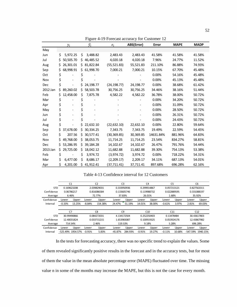
52

Figure 4-19 Forecast accuracy for Customer 12

Table 4-13 Confidence interval for 12 Customers

In the tests for forecasting accuracy, there was no specific trend to explain the values. Some

of them revealed significantly positive results in the forecast and in the accuracy tests, but for most

of them the value in the mean absolute percentage error (MAPE) fluctuated over time. The missing

value n in some of the months may increase the MAPE, but this is not the case for every month.

ABS(Error) Error MAPE MADP

May

Jun 5,972.25$ 3,488.82$ 2,483.43 2,483.43 41.58% 41.58% 41.58%

Jul 50,505.70$ 46,485.52$ 4,020.18 4,020.18 7.96% 24.77% 11.52%

Aug 26,301.01$ 81,822.84$ (55,521.83) 55,521.83 211.10% 86.88% 74.93%

Sep 68,998.91$ 61,998.70$ 7,000.21 7,000.21 10.15% 67.70% 45.48%

Oct -$ -$ - - 0.00% 54.16% 45.48%

Nov -$ -$ - - 0.00% 45.13% 45.48%

Dec -$ 24,198.77$ (24,198.77) 24,198.77 0.00% 38.68% 61.42%

2012 Jan 89,260.02$ 58,503.78$ 30,756.25 30,756.25 34.46% 38.16% 51.44%

Feb 12,458.00$ 7,875.78$ 4,582.22 4,582.22 36.78% 38.00% 50.72%

Mar -$ -$ - - 0.00% 34.20% 50.72%

Apr -$ -$ - - 0.00% 31.09% 50.72%

May -$ -$ - - 0.00% 28.50% 50.72%

Jun -$ -$ - - 0.00% 26.31% 50.72%

Jul -$ -$ - - 0.00% 24.43% 50.72%

Aug -$ 22,632.10$ (22,632.10) 22,632.10 0.00% 22.80% 59.64%

Sep 37,678.00$ 30,334.25$ 7,343.75 7,343.75 19.49% 22.59% 54.45%

Oct 207.56$ 30,577.41$ (30,369.85) 30,369.85 14631.84% 881.96% 64.83%

Nov 49,768.00$ 38,053.75$ 11,714.25 11,714.25 23.54% 834.27% 58.81%

Dec 53,286.95$ 39,184.28$ 14,102.67 14,102.67 26.47% 791.76% 54.44%

2013 Jan 29,725.00$ 18,042.12$ 11,682.88 11,682.88 39.30% 754.13% 53.38%

Feb -$ 3,974.72$ (3,974.72) 3,974.72 0.00% 718.22% 54.31%

Mar 6,477.00$ 8,686.17$ (2,209.17) 2,209.17 34.11% 687.13% 54.01%

Apr 4,201.00$ 41,912.41$ (37,711.41) 37,711.41 897.68% 696.28% 62.16%

𝑖 𝑖 𝑒𝑖

STD

Confidence

Average

Lower Upper Lower Upper Lower Upper Lower Upper Lower Upper Lower Upper

-0.33% 13.25% -8.84% 154.38% 24.47% 51.19% 14.01% 38.00% -0.61% 3.97% 2.81% 69.03%

STD

Confidence

Average

Lower Upper Lower Upper Lower Upper Lower Upper Lower Upper Lower Upper

-525.49% 1954.57% -0.91% 5.83% -45.87% 284.93% -0.91% 19.27% -0.11% 10.68% -547.59% 1940.15%

C1

0.169623208

0.06786217

6.46%

Confidence

Interval

0.119988732

26.01%

C2

2.039829031

0.816086584

72.77%

C6

0.827563311

0.331088197

35.92%

C7 C9

C4 C5

0.057213121

0.022889595

1.68%

0.333950936

0.133605746

37.83%

C3

0.299914867

Confidence

Interval

0.084272031

0.033715215

2.46%

C8

30.99490866

12.40031824

714.54%

C12

30.43617803

12.43867982

696.28%

1.653983087

119.53%

0.13478484

0.053924176

5.28%

C10

0.252250403

0.100919325

9.18%

C11

4.134172504

53

4.5 Conclusion

In this chapter, we demonstrate how to compute the forecast using our model. In Section

4.1, we introduce the basic information of the data set that we used. In Section 4.2, we explain the

differences between five models, especially with regard to the parameter in the distribution, the

input for the R matrix, and the parameter for smoothing the model. In Section 4.3 we implement

our data by computing the results for one of the customers for a specific month and year. We show

the process for using our model and explain the different payment patterns of individual customers.

This helped us to select the models that we used for forecasting. Section 4.4 demonstrates the results

obtained from the testing for the forecast.

By inputting the data into the combined model, we can observe that the combined model

which we created improves the forecast results. We can select the model by computing the inflow

R matrix, and then obtain the matrix of Difference. Then we calculate the average and the standard

deviations for the matrix of Difference as the criteria for selecting the model. Although the mean

absolute percentage error fluctuates over time, the mean absolute deviation percent (MADP)

remains within a certain range. The results from only four of the customers exceeded 50%; the

rest were quite low, fluctuating only within a small range. Also, in the process of recreating the

model we found that the parameters of Alpha and Beta will not converge over time. Thus, we

cannot set a specific value at the very beginning. We approach this by setting the range and

increment for the parameters and running the program with all of the combinations; thus, we obtain

the optimum solution.

54

Chapter 5

CONCLUSIONS AND FUTURE DIRECTIONS

5.1 Conclusions

This thesis refined the model by examining the payment behavior of each customer in the

company. According to their behavior, we selected a particular model to perform the forecast. The

combinations of the parameters, Alpha, Beta and shape parameters were calculated by going

through every combination that was within the range we set to obtain the forecast value with the

smallest average forecast error. Our model requires at least two months’ worth of data, and the

extra information that we obtain is from the payment behavior, which is the criterion that we used

to improve the forecast result. By studying the payment behavior of each customer, we can also

use this as a criterion by which to select suppliers. They could each be given a score based on their

payment behavior; if the score is below a certain level, then the company might wish to consider

changing the customer or reducing the order from that customer.

5.2 Future Directions

There are several possible extensions to the work presented in this thesis.

1. Find the formula for the relationship between customer behavior and the forecast model.

In this thesis, we first have to compute the Inflow R matrix, and calculate the average and

standard deviation, before deciding on the most appropriate model for the forecasting. It

may be possible to merge this in the model in order to obtain a more direct method for

performing the forecast.

55

2. Another possible extension to this work could be to investigate a method for determining

which model to use for dealing with a new customer. Our own model requires at least two

months’ data for forecasting; thus, it currently cannot be applied to new customers.

3. The relationship between each of the forecast methods and the company could be further

investigated. As we only tested 12 customers, there may be other significant scenarios that

we did not include in this thesis.

56

References

Gentry, J.A. and De La Garza,J. M. . (1985). A Generalized Model for Monitoring Accounts

Receivable. Financial Management, Vol. 14, No. 4 pp. 28-38.

Kallberg, J. G. and Saunders, A. (1983). Markov Chain Approaches to the Analysis of Payment

Behavior of Retail Credit Customers. Financial Management, Vol. 12, No. 2 ,pp. 5-14.

Accounts Receivable Analysis. (2015). Retrieved from Accounting Tools:

http://www.accountingtools.com/accounts-receivable-analysis

Baas, T. and Schrooten, M. . (2006). Relationship banking and SMEs: A theoretical analysis.

Small Business Economics, 27(2/3): 127-137.

Barbosa, P. S. F. and Pimentel, P. R. . (2001). A linear programming model for cash flow

management in the Brazilian construction industry. Construction Management and

Economics, 19, 469-479.

Barbosa, P.S.F. and Pimentel, P.R. (2001). A linear programming model for cash flow

management in the Brazilian construction industry. Construction Management and

Economics, 469-479.

Baumol, W. J. (1952). The transactions demand for cash: an inventory theoretic approach.

Journal f Economic, 66, 545-556.

Carpenter, M. D. and Miller,J. E. (1979). "A Reliable Framework for Monitoring Accounts

Receivable. Financial Managment, 37-40.

Corcoran, A. W. (1978). The use of exponentially-smoothed transition matrices to improve

forecasting of cash flows from accounts receivable. Management Science , 24(7): 732-

739.

Cyert, R. M., H. J. Davidson, et al. (1962). Estimation of the allowance for doubtful accounts by

Markov chains. Management Science, 287-303.

57

Fuchs, B. (2011). Best practices in cash flow forecasting.

Givoly, D. , Hayn, C., Lehavy, R. (2009). The Quality of Analysts’ Cash Flow Forecasts. THE

ACCOUNTING REVIEW, Vol. 84, No. 6 , pp. 1877–1911.

Gregory, G. (1976). Cash Flow Models: A Review. Journal of Management Science, Vol. 4, No.

6,pp.643-656.

Hofmann, E. (2003). The flow of financial resources in the supply chain : creating shareholder

value through collaborative cash flow management. In H. Kotzab, Eighth ELA Doctorate

Workshop 2003 (pp. 67-94). TU, Inst. für Betriebswirtschaftslehre (Darmstadt).

Hwee, N. G. and Tiong R. L. K. (2002). Model on cash flow forecasting and risk analysis for

contracting firms. International Journal of Project Management, 351–363.

Jackson, S. B. and Liu, X. (June 2010). The allowance for Uncollectible Accounts, Conservatism,

and Earnings Management. Jornal of Accounting Research, Vol. 48 No. 3 565-601.

Kallberg, J.G. and Saunders, A. (1983). Markov Chain Approaches to the Analysis of Payment

Behavior of Retail Credit Customers. Financial Management, 5-14.

Michalski, G. (2007). Portfolio management approach in trade credit decision making. Romanian

Journal of Ecomonic Forecasting, 3: 42-53.

Miller, M. H. and Orr, D. (1966). A model of the demand for money by firms. The Quarterly

Journal of Economics, 80(3): 413-435.

Pate-Cornell, M. E., G. Tagaras, et al. (1990). Dynamic optimization of cash flow management

decisions: A stochastic model. IEEE Transactions on Engineering Management, 37(3):

203-212.

Patinkin, D. (1965). Money, Interest andPrices, 2nd End. New York: Harper & Row.

Rinne, H. (2008). The weibull Distribution: A Hand Book. Chapman and Hall/CRC.

Saibeni, A. A. (2010). Forecasting Accounts Receivable Collections with Markov Chains and

Microsoft Excel. The CPA Journal , 66-71.

58

Skitmore, M. (1992). Parameter prediction for cash flow forecasting models. Construction

Management and Economics, 10, 397-413.

Srinivasan, V. and Kim, Y.H. (1986). Deterministic Cash Flow Management: State of the Art and

Research Directions. Journal of Management Science, 145-166.

Stone, B. K. (1976). The Payments-Pattern Approach to the Forecasting and Control of Account

Receivable. Financial Management, Vol. 5, No.3, 65-82.

Tangsucheeva, R. and V. Prabhu. (2014). Stochastic Financial analytics for cash flow forecast.

International Journal of Prediction Economics, 65-76.

Tsai, C. (2008). On supply chain cash flow risks. Science Direct, 1031-1042.