a state space model approach to functional time series …

A STATE SPACE MODEL APPROACH TOFUNCTIONAL TIME SERIES AND TIME SERIES

DRIVEN BY DIFFERENTIAL EQUATIONS

BY JIABIN WANG

A dissertation submitted to the

Graduate School—New Brunswick

Rutgers, The State University of New Jersey

in partial fulfillment of the requirements

for the degree of

Doctor of Philosophy

Graduate Program in Department of Statistics and Biostatistics

Written under the direction of

Professor Rong Chen

and approved by

New Brunswick, New Jersey

October, 2012

ABSTRACT OF THE DISSERTATION

A State Space Model Approach to Functional Time Series

and Time Series Driven by Differential Equations

by Jiabin Wang

Dissertation Director: Professor Rong Chen

This dissertation studies the modeling of time series driven by unobservable pro-

cesses using state space model. New models and methodologies are proposed and ap-

plied on a variety of real life examples arising from finance and biology. More specifically,

we mainly consider two types of time series: partially observed dynamic systems driven

by differential equations and functional time series driven by its feature process.

The first type of time series data is generated by a hidden dynamic process controlled

by some underlying differential equation with a set of unknown parameters. We propose

a state space approach to fit these models with observation data, which is only available

at sparsely separated time points as well as with measurement error, and estimate

the corresponding parameters. More specifically, we approximate the target nonlinear

deterministic/stochastic differential equations by difference equations and convert the

dynamic into a state space model(SSM), which is further calibrated by the likelihood

calculated from the filtering scheme. The first application converts the HIV dynamic

into a linear SSM and estimates all HIV viral dynamic parameters successfully without

many constraints. The second application focus on the well-studied ecological SIR

model. An efficient filtering scheme is proposed to overcome the difficulty caused by

the sparsity of the observed data. The methodology is illustrated and evaluated in the

ii

simulation studies and the analysis of bartonella infection data set.

The second part of the thesis applies state space model approach on functional time

series driven by its feature process, with illustration on two financial data sets. We

first find the underlying feature process and build its transitional relationship, which

provides the basis to build a SSM form. Then we infer the unknown parameters from

likelihood calculated from the filtering scheme. The first application analyzes the U.S.

treasury yield curve from January 1985 through June 2000 and proposed a two-regime

AR model on its feature process: level, slope and curvature of the yield curve. The

second application applies the framework on the daily return distributions of the 1000

largest capitalization stocks from 1991 to 2002. A novel skew-t distribution is used

to fit the target distribution and to extract the parameters of the distribution as the

feature process, which is further fitted by a vector moving average model. Compared

to competing models, our model shows superior prediction performance in both appli-

cations.

iii

Acknowledgements

First I would like to express my deepest gratitude to my advisor, Professor Rong Chen,

for all the guidance, help and encouragement, for teaching me how to think and write

academically, for his invaluable insights and suggestions, which gave rise to many in-

teresting ideas and fruitful results.

I also thank Professor Hua Liang and Professor Javier Cabrera for past collabora-

tions. I learned a lot from the discussions.

I would like to thank the faculties in the department of statistics, Professor Minge

Xie, Professor Rebecka Jornsten, Professor Cun-Hui Zhang, Professor Tong Zhang, Pro-

fessor William E. Strawderman, Professor Harold B. Sackrowitz, and Professor Richard

F. Gundy for teaching me statistics and inspiring my interest in statistical research.

Especially I am grateful to Professor Xie Minge, Professor Han Xiao and Professor

Xiaodong Lin for serving in my PhD committee and the precious advice they gave on

this dissertation.

This is also an opportunity to thank my former and current colleagues in the statis-

tics program: Wentao Li, Dungang Liu, Wei Li, Kuo-mei Chen, Tingni Sun, Wenqian

Qiao, Yingqiu Ma and Shuhao Chen. I enjoyed the discussions with them on various

topics and is grateful to be a member of this fantastic group.

Finally I want to thank my parents for their life long support and love.

iv

Dedication

For my parents Wang Dingqing and Liu Xianglang.

v

Table of Contents

Abstract . . . . . . . . . . . . . . . . . . . . . . . . . . . . . . . . . . . . . . . . ii

Acknowledgements . . . . . . . . . . . . . . . . . . . . . . . . . . . . . . . . . iv

Dedication . . . . . . . . . . . . . . . . . . . . . . . . . . . . . . . . . . . . . . . v

1. Introduction . . . . . . . . . . . . . . . . . . . . . . . . . . . . . . . . . . . 1

1.1. State Space Form . . . . . . . . . . . . . . . . . . . . . . . . . . . . . . . 2

1.2. Hidden Process . . . . . . . . . . . . . . . . . . . . . . . . . . . . . . . . 4

1.3. Outline of Thesis . . . . . . . . . . . . . . . . . . . . . . . . . . . . . . . 5

2. Methodology Review . . . . . . . . . . . . . . . . . . . . . . . . . . . . . . 8

2.1. System of First Order Differential Equation . . . . . . . . . . . . . . . . 8

2.1.1. Solution of Linear ODE . . . . . . . . . . . . . . . . . . . . . . . 9

2.1.2. Discretization of ODE . . . . . . . . . . . . . . . . . . . . . . . . 9

2.1.3. Discretization of SDE . . . . . . . . . . . . . . . . . . . . . . . . 11

2.2. State Space Model . . . . . . . . . . . . . . . . . . . . . . . . . . . . . . 13

2.2.1. Kalman Filter . . . . . . . . . . . . . . . . . . . . . . . . . . . . . 13

2.2.2. Extended Kalman Filter . . . . . . . . . . . . . . . . . . . . . . . 15

2.2.3. Unscented Kalman Filter . . . . . . . . . . . . . . . . . . . . . . 16

2.2.4. Particle Filter . . . . . . . . . . . . . . . . . . . . . . . . . . . . . 17

2.2.5. Computational Aspects . . . . . . . . . . . . . . . . . . . . . . . 19

2.2.6. Fixed Parameter Problem . . . . . . . . . . . . . . . . . . . . . . 20

2.3. Prior Approaches on Differential Equation Calibration . . . . . . . . . . 22

2.3.1. Parameter Estimation for ODE . . . . . . . . . . . . . . . . . . . 22

2.3.2. Maximum Likelihood Estimation for SDE . . . . . . . . . . . . . 24

2.3.3. State Space Model Approach . . . . . . . . . . . . . . . . . . . . 24

vi

2.4. Linear Time Series Analysis . . . . . . . . . . . . . . . . . . . . . . . . . 25

2.4.1. Vector Autocorrelation Model . . . . . . . . . . . . . . . . . . . . 25

2.4.2. Nonlinear Time Series Analysis . . . . . . . . . . . . . . . . . . . 26

3. A State Space Model Approach for HIV Infection Dynamics . . . . 28

3.1. Background . . . . . . . . . . . . . . . . . . . . . . . . . . . . . . . . . . 28

3.2. Model Representation . . . . . . . . . . . . . . . . . . . . . . . . . . . . 29

3.2.1. ODE to SSM . . . . . . . . . . . . . . . . . . . . . . . . . . . . . 29

3.2.2. SSM vs Runge-Kutta . . . . . . . . . . . . . . . . . . . . . . . . 33

3.2.3. Approximation Error . . . . . . . . . . . . . . . . . . . . . . . . . 33

3.2.4. B-Spline Approximation . . . . . . . . . . . . . . . . . . . . . . . 34

3.3. Model Estimation . . . . . . . . . . . . . . . . . . . . . . . . . . . . . . . 34

3.4. Simulation Studies . . . . . . . . . . . . . . . . . . . . . . . . . . . . . . 36

3.5. Real Data Analysis . . . . . . . . . . . . . . . . . . . . . . . . . . . . . . 38

3.5.1. Model Specification and Estimation . . . . . . . . . . . . . . . . 38

3.5.2. Results and Discussions . . . . . . . . . . . . . . . . . . . . . . . 39

3.6. Conclusion and Discussion . . . . . . . . . . . . . . . . . . . . . . . . . . 42

4. A State Space Model Approach to Infectious Disease Spread Dynam-

ics . . . . . . . . . . . . . . . . . . . . . . . . . . . . . . . . . . . . . . . . . . . . 44

4.1. Background . . . . . . . . . . . . . . . . . . . . . . . . . . . . . . . . . . 44

4.2. Model Representation . . . . . . . . . . . . . . . . . . . . . . . . . . . . 46

4.2.1. Deterministic Model . . . . . . . . . . . . . . . . . . . . . . . . . 46

4.2.2. Stochastic Model . . . . . . . . . . . . . . . . . . . . . . . . . . . 47

4.3. Model Estimation . . . . . . . . . . . . . . . . . . . . . . . . . . . . . . . 49

4.3.1. ODE-PF . . . . . . . . . . . . . . . . . . . . . . . . . . . . . . . 49

4.3.2. Model Estimation for Stochastic SIR . . . . . . . . . . . . . . . . 51

4.3.3. Computation Aspects . . . . . . . . . . . . . . . . . . . . . . . . 53

4.4. Simulation Studies . . . . . . . . . . . . . . . . . . . . . . . . . . . . . . 55

4.4.1. ODE version of SIR . . . . . . . . . . . . . . . . . . . . . . . . . 55

vii

4.4.2. SDE Version of SIR . . . . . . . . . . . . . . . . . . . . . . . . . 57

4.5. Real Data Analysis . . . . . . . . . . . . . . . . . . . . . . . . . . . . . . 60

4.5.1. Model Specification and Estimation . . . . . . . . . . . . . . . . 60

4.5.2. Results and Discussions . . . . . . . . . . . . . . . . . . . . . . . 61

4.6. Conclusion and Discussion . . . . . . . . . . . . . . . . . . . . . . . . . . 61

5. Functional Time Series driven by its Feature Process . . . . . . . . . 66

5.1. Background . . . . . . . . . . . . . . . . . . . . . . . . . . . . . . . . . . 66

5.2. Model Set-up . . . . . . . . . . . . . . . . . . . . . . . . . . . . . . . . . 69

5.2.1. FTS Driven by Finite Dimensional Dynamic Processes . . . . . . 70

5.2.2. DTS Driven by Finite Dynamic Processes . . . . . . . . . . . . . 71

5.3. Application: Modeling and Forecasting Treasury Yield Curve . . . . . . 72

5.3.1. Yield Curve Shape . . . . . . . . . . . . . . . . . . . . . . . . . . 72

5.3.2. FTS-FP for Modeling Yield Curve . . . . . . . . . . . . . . . . . 74

5.3.3. Model Estimation . . . . . . . . . . . . . . . . . . . . . . . . . . 75

5.3.4. Model Comparison . . . . . . . . . . . . . . . . . . . . . . . . . . 76

5.4. Application: Cross-sectional stock return distributions . . . . . . . . . . 78

5.4.1. Fitting of Skew T-distribution . . . . . . . . . . . . . . . . . . . 78

5.4.2. DTS-FP for Cross-Sectional Return Distribution . . . . . . . . . 81

5.4.3. Prediction Performance Comparison to Simpler Models . . . . . 83

5.5. Conclusion . . . . . . . . . . . . . . . . . . . . . . . . . . . . . . . . . . 84

viii

1

Chapter 1

Introduction

The need for monitoring and analyzing sequential data arises in many scientific and

industrial problems. Time series analysis deals with such records collected over time,

with the distinguishing feature of dependence among records. The fundamental task

of time series analysis is to reveal the law that governs the observed time series and

hence to understand the dynamics, forecast future event and control future events via

intervention. Time series analysis relies on statistical modeling. A proper model for a

time series should possess the salient feature of the observed data.

This dissertation focuses on modeling of time series driven by another unobservable

process and utilizes the proposed models and methodologies on a wide variety of real

life examples arising from both financial and biological area. More specifically, we

mainly consider two types of time series: partially observed dynamic systems driven by

differential equations and functional time series driven by its feature process.

The first topic deals with the case when several state variables interact and change

over time but only part of them or linear transformations of them are observed. Usually

the observed data are corrupted with noise and observed at discrete time with possible

long time interval. The dynamic process is usually modeled by differential equations.

This occurs in many applications. For example, the total cells and virus number in

human body are the result of full interacting dynamic between the uninfected cell,

infected cells and virus. Patients are tested on a regular basis for the total number of

uninfected and infected cells number and the number of virus number. The interest is

then to model the underlying virus progress with the observed data so one could make

better prediction on the virus number.

The second topic is driven by the need to model modern data collection with more

2

and more observations in the form of functions, images and distributions. For example,

in insurance industry mortality rate as a function of age(mortality curve) changes over

time. In banking and financial industry, term structure of interest rate(yield as a func-

tion of time to maturity of a bond) changes over time, implied volatility surface(implied

volatility as a function of an option’s strike price and time to maturity) changes over

time. There are countless other such examples in applications. Many of these function

process could be well characterized by its underlying feature process. For example,

the interest rate curve could almost always be fully represented by its level, slope and

curvature through certain parametric form. The level, slope and curvature process are

then the feature process that drives the observed interest rate curve. When such ob-

servations are observed over time and exhibit dynamic behaviors, time series models

in the functional space becomes a necessary and useful tool for analyzing such data as

well as making forecasts of the future.

The main tool used to study the two topics is the state space model and its related

filtering scheme, Kalman Filter for the linear gaussian form and Particle Filter for

other cases. The following contents give a brief introduction of the state space form

and conversion of the problem to the form. In the end of this chapter, the outline of

this thesis is also provided.

1.1 State Space Form

Let the observed time series be YT1 = Y1, · · · ,YT , where T is the number of

observations in the sequence. Each observation at time t, Yt, is a real-valued vector

of dimension l. Denoting Yt1 = Y1, · · · ,Yt, the joint probability of the observed

sequence can always be represented as:

P (Y1, · · · ,YT ) = P (Y1)

T∏t=2

P (Yt|Yt−11 ). (1.1)

In general, the models considered in time series analysis will put some constraint

on P (Yt|Yt−11 ) to get a concise form of the relationship between Yt and the entire

history of the time series. Conventional time series models aim to build this compact

relationship using only the past history of observations Yt−11 but in reality there are a

3

wide class of data generated from a dependence dynamic controlled by another hidden

dynamic process XT1 , with dimension k. Under this assumption, the following general

state space model is considered:

Yt = gθ(Xt) + ut

Xt = fθ(Xt−1) +wt

ut

wt

∼ P

0

0

,

Ut 0

0 Wt

, (1.2)

where Xt and Yt are the unobserved state vector and the observation vector respec-

tively, θ represents all unknown parameters in the model, function gθ quantifies the

relationship between Xt and mean of Yt while fθ depicts how the mean of Xt is deter-

mined by Xt−1. The observational noise ut and wt are assumed to be independently

distributed with measurement error distribution and state equation distribution of zero

mean and variance Vt and Wt respectively, which may or may not depend on θ. The

initial state distribution is assumed to be X0 ∼ P0(X0; θ).

Filtering aims to calculate P (Xt|Yt1) and further to estimate functions of the current

underlying state given the previous data. This could be recursively calculated by,

(Sorenson; 1988):

P (Xt|Yt−11 ) =

∫P (Xt|Xt−1)P (Xt−1|Yt−1

1 )dXt−1, (1.3)

P (Xt|Yt1) = c−1

t P (Yt|Xt)P (Xt|Yt−11 )

ct = P (Yt|Yt−11 ) =

∫P (Yt|Xt)P (Xt|Yt−1

1 )dXt.(1.4)

Equation (1.3) is called prediction equation and equations in (1.4) are called filtering or

update equation. These two equations together give a recursive solution to the filtering

problem. Most of the thesis concerns the inference of model parameters based on the

above probability, which is usually a side product of the filtering scheme as follows:

p(Y1, · · · ,YT ) = p(Y1)

T∏t=2

p(Yt|Yt−11 ) =

T∏t=1

ct. (1.5)

When model (1.2) takes a linear form with gaussian noise, the above recursive

formulas can be explicitly written out and are the acclaimed Kalman Filter. In other

cases the integrations involved are still intractable and require more advanced filtering

schemes such as Particle Filter.

4

1.2 Hidden Process

The hidden dynamic process, either the precess specified by the differential equation or

the feature process, constitutes the state transition equation in the state space form.

The feature process usually takes form as a auto-correlated time series model, hence

is straight forward to be written as a generalized state space equation.

Yt = gθ(Xt) + εt, εt ∼ P yθ (Xt),

Xt = fθ(Xt−p, · · · ,Xt−1, et−q, · · · , et−1),

(1.6)

where P yθ is the distribution for measurement error εt and fθ is a known function,

which both depend on a set of unknown parameters θ. For example, one can use a

vector ARMA(p,q) for the state equation. et is white noise and εt is the measurement

error.

For the underlying process specified by a first order differential equation as follows:

dXt = f∗(Xt)dt, (1.7)

when f∗(Xt) is constant, the system is linear. Otherwise, it is a nonlinear system.

This continuous process could be further discretized and approximated by an ordinary

difference equation.

Xt+∆t = Xt + e(Xt,∆t). (1.8)

This approximation is exact when the ODE is linear but more often there is an approx-

imation error depending on the states and step size.

Random perturbations in the state process lead to adding a noise term in the dif-

ference equation:

Xt+∆t = Xt + e(Xt) +Σ(Xt, t)vt, (1.9)

where vt is a Gaussian noise with variance ∆t and the whole random perturbation

term has a variance of ∆tΣ(X, t)Σ(X, t)′ that depends on current state, time and the

length of time interval. The above representation corresponds to a stochastic differential

equation(SDE) of the state process, i.e.,

dXt = f∗(Xt)dt+Σ(Xt)dWt, (1.10)

5

where Wt is a standard Wiener process.

The observed time series are usually measured at sparse time points tjNj=1 with

some background noise.

Ytj = g(Xtj ) + εtj , εtj ∼ P yθ (Xtj ).

Then the state space model for time series driven by differential equations is as

follows:

Ytj = g(Xtj ) + εtj , εtj ∼ P yθ (Xtj ),

Xt = fθ(Xt−1) + ηt ηt ∼ P xθ (Xt−1),

X0 ∼ P0(X0; θ).

(1.11)

1.3 Outline of Thesis

Given sequentially observed data generated from a dynamic system, characterized by

either a differential equation or a specific form or distribution, the framework of calibra-

tion via state space model then consists of three steps: converting the dynamic system

into a state space model, using filtering scheme to obtain the likelihood approximation

and locating the maximum likelihood estimator. An outline of the subsequent chapter

contents is as follows:

Chapter 2 reviews the literature on filtering algorithms in state space model. The

main breakthrough in the filtering theory is Kalman filter (Kalman; 1960), a recursive

algorithm for filtering and estimation of linear and Gaussian state space models. Un-

like the linear gaussian state space model, which have explicit optimal filter (Kalman

Filter,Kalman (1960)), the nonlinear state space model usually have no explicit form

as to filtering. Extensive statistical researches exist to overcome this nonlinearity, for

example extended Kalman filter (EKF) and Unscented kalman filter (UKF). Another

type of filtering method for the nonlinear state space model, particle filter, has been

proposed and studied in engineering and statistics. The idea is to approximate the

target distribution(usually P (X1, · · · ,Xt|Yt1)) by a set of properly weighed sample

(Xj1:t, w

jt ), which is drawn sequentially from some trial distribution. These filters

are briefly reviewed together with prior researches in differential equation calibration.

6

Chapter 2 also give a brief coverage of linear time series model and differential equation

discretization scheme.

Chapter 3 presents the framework to modeling the HIV dynamic from limited clini-

cal data. The observed clinical time series data can be viewed as generated by a hidden

dynamic process controlled by some nonlinear differential equation with a set of un-

known parameters. We propose a state space approach to link these models with clinical

data and estimate corresponding parameters. Specifically, we approximate the target

nonlinear differential equations by difference equations and convert the dynamic into

a gaussian linear state space form, which could further be calibrated by the prediction

error decomposition from Kalman Filter. To illustrate the proposed method, we apply

it to the clinical data of two individual HIV infected patients treated with antiretroviral

therapies. The proposed model and methodology provide an alternative tool in HIV

dynamic modeling and can be easily applied in other biomedical system characterized

by dynamic systems.

Chapter 4 shows the calibration of the well-studied ecological SIR model via con-

version to a nonlinear state space model. An adapted filtering scheme is proposed

to efficiently sample and to approximate the target likelihood. SIR model is a set of

differential equations that describes the dynamic of the spread of an infectious dis-

ease. Depending on the stage of the disease, the whole population is assigned to three

different subgroups: susceptible(S), infectious(I), and recovered(R). Each individual

typically progresses from susceptible to infectious to recovered, which resulted in a dy-

namic course of the three group number over time. We convert the target nonlinear

differential equations into a nonlinear state space form and apply an efficient filtering

algorithm to deal with the large time interval problem in stochastic SIR model. To il-

lustrate the proposed method, we apply it to the simulated data sets and the bartonella

infection data set.

In chapter 5, two examples from finance area are considered, as illustration of apply-

ing state space model in functional time series analysis. The main challenge of modeling

functional time series is the change of dynamic in both dimensionality(function) and

time. This dissertation takes a two-step approach by first finding the low dimensional

7

representation of the high dimensional data, which is named as its feature process, and

then exploring the dynamic of the feature process over time. By reducing the dimen-

sionality without much information loss, the modeling of a low dimensional feature

process now becomes a more feasible task. The forecasting is therefore a corresponding

two-step process by forecasting the feature process first and then predicting the original

high dimension time series through the relationship. In a variety of circumstances, this

could further be formatted as a general state-space model (SSM), hence estimation and

forecasting can both be done in a one-step approach with more efficiency. Based on

the above idea, we propose a functional time series model driven by the feature process

model (FTS-FP). The structure between observed functional data and latent process

at each time point is determined by known knowledge or by choosing a form of best

fit function from a pre-specified groups of function forms. This model achieves model

reduction and provides a coherent description of the dynamic system and an efficient

way to do prediction. When the functional time series are density functions, a corre-

sponding model called distributional time series driven by the feature process model

(DTS-FP) is proposed. These two models are then applied to model the dynamic of 17

dimension yield curve for U.S. Treasure Bond and that of cross-sectional stock returns

respectively.

8

Chapter 2

Methodology Review

This chapter is devoted to a review of the methodologies used throughout this thesis.

The main focus is in various filtering algorithms for the linear and non-linear state space

model. The classic linear time series model and the first order differential equation

system are also briefly reviewed.

2.1 System of First Order Differential Equation

Systems of ordinary differential equations arise naturally in problems involving several

dependent variable, each of which is a function of a single independent variable. Many

dynamic systems evolving with time could be characterized by such system, with the

independent variable being time and the variables of interest being the set of dependent

functions. Among them, first order differential equation system links the instaneous

change of the variables with time and all dependent variables. It has the following form:

dX1,t

dt= f∗

1 (X1,t, · · · , XK,t),

· · ·dXK,t

dt= f∗

K(X1,t, · · · , XK,t),

(2.1)

where X1,t, · · · , XK,t are the variable of interest in the dynamic system. Denoting

Xt = (X1,t, · · · , XK,t), the initial condition is:

Xt0 = X0. (2.2)

Model (2.1) can always be represented by a the matrix form:

Xt +P[Xt, t]Xt = Q[Xt, t], (2.3)

9

2.1.1 Solution of Linear ODE

When P[Xt, t] = P and Q[Xt, t] = Q do not depend on Xt, the system is linear and

well studied (Boyce and DiPrima; 2004).

It is convenient to first consider the homogeneous equation, with Q = 0:

Xt +PXt = 0, (2.4)

The solution ϕ(t) could usually be expressed as:

ϕ(t) = c1X(1)t + c2X

(2)t + · · ·+ cKX

(K)t , (2.5)

where X(1)t ,X

(2)t · · ·X(K)

t are solutions of the system (2.3) and linearly independent, ck

are suitable coefficients determined by the initial condition for the system.

In the simplest case where P is have different real eigenvalues ,

X(k) = ϵ(k)erkt, k = 1, · · · ,K, (2.6)

where rk is the k-th eigenvalue of P and ϵ(k) is the eigenvector associated with it.

Solutions with constant P but more complicated eigenvector conditions can be found

in Boyce and DiPrima (2004).

Suppose the solutions to 2.4 are available and are put together as a matrix Φ(t) =

(X(1)t , · · · ,X(K)

t ), then the general solution for the system 2.3 by the method of variation

of parameters is:

Xt = Φ(t)c+Φ(t)

∫ t

Φ−1(s)Q(s)ds, (2.7)

where c is then determined by the initial condition.

2.1.2 Discretization of ODE

Though mathematically solving the system provides a thorough understanding of the

system, most problems can not be solved analytically. With the advent of high-speed

computers, the use of numerical methods to solve differential equation problems has

become commonplace. The main idea is to convert the original differential equation to

a difference equation and progress stepwise from the starting point to get the discretized

path.

10

Consider a given discretization 0 < h < 2h < · · · < Nh = T < inf of the time inter-

val [0,T]. The interest is to generate X(h; t0,X0),X(2h; t0,X0), · · · ,X(Nh; t0,X0) at

the above discrete times to approximate the underlying process Xtrue(nh; t0,X0) satis-

fying 2.1. For simplicity, equidistant time discretizations, where h is the discretization

step, is used for this thesis. In the later notation, ∆t sometime is also used to represent

the discretization step. The following derivation is based on scaler Xt, which could be

easily extended to multivariate cases. The local discretization and global discretization

error at the n-th time step are defined as:

ln+1 = X(tn+1; t0, X0)−Xtrue(tn+1; tn, Xn),

en+1 = X(tn+1; t0, X0)−Xtrue(tn+1; t0, X0).

To measure the accuracy of different schemes, order of convergence is defined as the

largest γ such that there exists a constant C < inf and :

eN ≤ Chγ .

Scheme with a larger order of convergence provides quicker convergence to the true

path as the discretization step gets smaller.

Taylor expansion around current state value Xt provides a fundamental basis for all

schemes:

Xt+h = Xt +dXt

dth+ · · ·+ 1

p!

dpXt

dtphp +

1

(p+ 1)!

dp+1X∗t

dtp+1hp+1, (2.8)

where t < X∗t < t+ h. It yields the p-th order truncated Taylor method by evaluating

the first p differential terms at Xtn and ignore the error term. This method obviously

has a local discretization error of order p+1. Under appropriate conditions, it can be

shown to have a global discretization error of p. A simple example is the Euler scheme

with a global convergence rate of 1 as follows:

Xt+h = Xt + hf∗θ (Xt, t) (2.9)

Though p-th order truncated Taylor method has intuitive and easy derivation, it

has complex computation and hence not applicable in practice. More convenient and

applicable methods are the one-step methods with the following form:

Xt+h = Xt + hΨθ(Xt, t) + ηt. (2.10)

11

The standard procedure with it is to first pose certain function form of Ψθ(Xt, t),

with several unknown constants, then derive the constants by comparing it to a trun-

cated Taylor method till certain order of its discretization error is satisfied. Runge-

Kutta methods fall into this class. The family of second order Runge-Kutta methods

are derived from the form:

Ψθ(Xt, t) = αf∗θ (Xt, t) + βf∗

θ (Xt + δhf∗θ (Xt, t), t+ δh), (2.11)

with the constraint α+β = 1 and δβ = 1/2. The fourth order Runge-Kutta method(RK4)

takes the form

Ψ(Xt, t) =1

6(k1,t + 2k2,t + 2k3,t + k4,t),

k1,t = f∗(tk, Xt), k2,t = f∗(tk +h

2, Xt +

h

2k1,t),

k3,t = f∗(tk +h

2, Xt +

h

2k2,t), k4,t = f∗(tk + h,Xt + k3,t).

Sometime it is of interest to write the relationship between Xt+h and Xt in explicit

terms, like the Euler scheme, while achieving a higher order. A general way to do so

for ODE (2.3) is proposed in Freed and Walker (1991):

Xt+h = exp(−P[Xt∗ , t]h)Xt + I− exp(−P[Xt∗ , t]h)P−1[Xt∗ , t]Q+O[∂

∂t

Q

P[Xt∗ , t]h2].

(2.12)

where t∗ can either be t + h or t, which corresponds to implicit and explicit approxi-

mation respectively. This approximation is exact for linear ODE.

2.1.3 Discretization of SDE

AK-dimensional stochastic process (X1,t, · · · , XK,t) driven by m independent (W1,t, · · · ,Wm,t)

Wiener process are generally depicted as:dX1,t

· · ·

dXK,t

=

f∗1,t(t,Xt)

· · ·

f∗K,t(t,Xt)

dt+

σ1,1(t,Xt) · · · σ1,m(t,Xt)

· · ·

σK,1(t,Xt) · · · σK,m(t,Xt)

dW1,t

· · ·

dWm,t

. (2.13)

In general, one does not know much about the solution of a given SDE. Some

discretization schemes could be employed to discover some of its properties. We show

12

them as follows for one dimensional Xt With the same equidistant time discretiztion

step h, one shall generate X(h; t0, X0) < X(2h; t0, X0) < · · · < X(Nh; t0, X0) at the

discrete times to approximate the underlying process Xtrue(nh; t0, X0) satisfying the

equation (2.13). Order of strong convergence is used to assess and classify different

discrete-time approximations. It is defined as the largest γ such that there exists a

constant C < inf and a δ0 > 0 satifying:

ϵ(h) = E(|XT (h)−XtrueT |) ≤ Chγ ,

for each h ∈ (0, δ0)

Just like the deterministic Taylor formula as an indispensable tool in ODE dsi-

cretization, there is an expansion with similar structure for the stochastic case. Such a

stochastic Taylor expansion is the Wagner-Platen expansion, which was first derived in

W. Wagner (1978) and emerges from an iterated application of the Ito formula. For il-

lustration purpose, we only shows the expansion for K=m=1. More detailed derivation

and expansion on multiple dimension could be found in Kloeden and Platen (1992).

When k=m=1 and f(t,Xt) and σ(t,Xt) only depends on time through Xt, equation

(2.13) reduces to

dXt = f∗(Xt)dt+ σ(Xt)dWt, (2.14)

and has Wagner-Platen expansion as:

Xt+h = Xt+f∗(Xt)

∫ t+h

tdt+σ(Xt)

∫ t+h

tdWt+σ(Xt)

dσ(Xt)

dXt,

∫ t+h

t

∫ s

tdWzdWs+R

(2.15)

where multiple Ito integrals are ∫ t+h

tdt = h,∫ t+h

tdWt = W (t+ h)−W (t),∫ t+h

t

∫ s

tdWzdWs =

1

2(W (t+ h)−W (t))2 − h,

and R consists of higher order Ito integrals with nonconstant integrand. The above ex-

pansion yields two of the most used scheme for SDE approximation: Euler and Milstein

13

scheme, which have strong order of 1/2 and 1 respectively.

Xt+h = Xt + hf∗(Xt) + σ(Xt)∆W, ∆W ∼ N(0, h),

Xt+h = Xt + hf∗(Xt) + σ(Xt)∆W +1

2σ(Xt)

dσ(Xt)

dXt((∆W )2 −∆), ∆W ∼ N(0, h).

In the general multi-dimensional case with m > 1 and d > 1, the kth component of

the Euler and Milstein scheme have the form:

Xk,t+h = Xt + hfk(Xt) +

m∑j=1

σk,j(Xt)∆Wj , ∆Wji.i.d. ∼ N(0, h),

Xk,t+h = Xt + hfk(Xt) +m∑j=1

σk,j(Xt)∆Wj

+

m∑j1,j2=1

1

2(

K∑k=1

σk,j1(Xt)dσk,j2(Xt)

dXt)∫ t+h

t

∫ s

tdWj1,zdWj2,s.

2.2 State Space Model

A state-space model (SSM) describes the process of the observed time series data as

being driven by some unobservable latent state variables. It consists of an observation

equation and a state transitional equation. A general state-space model is written as

the form (1.2).

2.2.1 Kalman Filter

A linear state-space model with Gaussian noise is generally written as:

Xt = Λt + FtXt−1 + ut

Yt = GtXt +wt

ut

wt

∼ N

0

0

,

Ut 0

0 Wt

, (2.16)

where Xt is the unobserved state vector, Yt is the observation vector, Λt, Ft, and Gt

are matrices known at time t, except a set of parameters. Here the observation noise

Wt and the state noise Ut are assumed to be normally distributed and independent.

Kalman filter (Kalman; 1960) is a recursive algorithm for filtering and estimation

of linear and Gaussian state space models. Here we give a brief review of this algo-

rithm. Details can be found in Harvey (1989) and Durbin and Koopman (2000). Since

the conditional distribution of Xt given all previous observed data is Gaussian, one

14

only needs to obtain its mean and covariance matrix. Denote µt|t = E(Xt|Y1, . . . ,Yt)

and Σt|t = Cov(Xt|Y1, . . . ,Yt), the Kalman recursion for model (2.16) proceeds by

updating µt|t and Σt|t as follows:

Pt+1|t = FtΣt|tFTt +Ut, µt+1|t = Λ+ Ftµt|t, (2.17)

St+1|t = GPt+1|tGT +Wt, et+1 = Yt+1 −GTµt+1|t,

µt+1|t+1 = µt+1|t +Pt+1|tGTS−1

t+1|tet+1, Σt+1|t+1 = Pt+1|t −Pt+1|tGTS−1

t+1|tGPt+1|t,

(2.18)

where et+1 and St+1|t are the prediction error and prediction error variance respectively.

When the initial state vector has density N(µ0,Σ0), the likelihood by prediction error

decomposition are written as

L(Y|Θ) =

n∑t=1

log p(Yt|Y1, . . . ,Yt−1) = −np

2log 2π − 1

2

n∑t=1

(log |St|t−1|+ eTt S−1t|t−1et).

(2.19)

When little information is known about the initial state vector, diffuse initialization

(Σ0 → ∞) could be used and a modified version of the above likelihood could be applied

(Durbin and Koopman; 2001).

While equations (2.17-2.18) give a recursive solution to the filtering problem, they

could also be easily adapted to prediction and smoothing. To simplify notation, we

use Dk to represent all the measurement Yt up to time k. To predict a future state

distribution given the current observation, P (Xl|Dk), l > k, one only needs to run

equations 2.17-2.18 till time k and only equation 2.17 for all time points beyond k

till l. For smoothing, which concerns the distribution of a former state given current

observation P (Xl|Dk), l < k, it could be carried out by enlarging the state space to

X∗t = (Xt,Xl). Then the state space model changes to:

X∗t =

Λt

0

+

Ft 0

0 I

X∗t−1 +

Ut

0

,

Yt =(Gt 0

)X∗

t +Wt.

(2.20)

15

The whole filtering process starts from time l and X∗l is initialized with mean (µl|l,µl|l)

and covariance matrix: Σl|l Σl|l

Σl|l Σl|l

.

The Kalman Filter equations are then applied to this model to give the mean and co-

variance matrix of the new state X∗t conditioned on all the observation till time k. They

could be further split to give only the mean and covariance matrix of P (Xl|Dk), l < k.

2.2.2 Extended Kalman Filter

A more general state space model usually takes a nonlinear form as in model (1.2).

Extended Kalman Filter(EKF) attacks this problem by linearizing the state and obser-

vation equation and applying the Kalman Filter on the linearized problem.

Assuming µt−1|t−1 and µt|t−1 are available, the state equation and measurement

equation could be linearized by Taylor expansion at around µt−1|t−1 and µt|t−1 respec-

tively:

Xt = f(µt−1|t−1) + Ft(Xt−1 − µt−1|t−1) + ut,

Yt = g(µt|t−1) +GtXt +wt

(2.21)

where

Ft =∂f

∂X|µt−1|t−1

, Gt =∂g

∂X|µt|t−1

. (2.22)

Kalman filter together with these linearized equations then give the EKF equations:

Pt+1|t = FtΣt|tFTt +Ut, µt+1|t = f(µt|t),

St+1|t = GtPt+1|tGTt +Wt, et+1 = Yt+1 − g(µt+1|t)−GT

t µt+1|t,

µt+1|t+1 = µt+1|t +Pt+1|tGTt S

−1t+1|tet+1, Σt+1|t+1 = Pt+1|t −Pt+1|tG

Tt S

−1t+1|tGtPt+1|t.

(2.23)

The main problem with EKF is the linearisation inaccuracy, depending on ||Xt−1−

µt−1|t−1||2 and ||Xt−µt|t−1||2 as well as the degree of non-linearity in f and g. Several

possible improvements are proposed to reduce the linearisation error. Among them,

one way (Denham and Pines; 1966) is to linearize the equation at around µt−1|t instead

of µt−1|t−1. This is motivated by the fact that with more observations available, the

smoothing state mean at time t is usually more accurate than filtering state mean.

16

As such the linearisation accuracy should be improved. This approach is called the

iterated EKF. Another suggestion (Sorenson and Stubberud; 1968a) is to add more

terms in the taylor expansion. This is intended to reduce the error in replacing linear

equation to approximate nonlinear f and g, however usually with more complication

and increased computational load. A comparison of the three approaches-EKF, iterated

EKF and adding more terms in expansion are presented on in Wishner et al. (1969).

The results show that overall iterated EKF provided the best results. With more terms

in expansion, the results are slightly more accurate than EKF but take more time to

run.

2.2.3 Unscented Kalman Filter

Instead of relying on linearization employed by EKF, the unscented Kalman filter(UKF)

use a deterministic sampling scheme called ”unscented transformation” to overcome the

difficulty in getting the mean and variance of f(µt−1|t−1) and g(µt|t−1). It is initially

proposed by Julier (1997) to extend kalman filter in nonlinear state space model and

shows to be superior to EKF in the study (Julier and Uhlmann; 2004).

Unscented transformation is a deterministic approximation method to find the mean

and variance y = f(Z), where f is one nonlinear function and Z is a nz dimensional

random variable with mean µz and Σz. The scaled unscented transform is given by

Julier and Industries (2002):

y0 = µz

yi = µz + (√

(nz + λ)Σz)i, i = 1, ..., nz,

yi = µz − (√

(nz + λ)Σz)i, i = nz + 1, ..., 2nz,

Wm0 =

λ

nz + λ,

W c0 =

λ

nz + λ+ (1− α2 + β),

Wmi = W c

i =1

2(nz + λ)i = 1, · · · , 2nz,

(2.24)

where λ = α2nz − nz. α and β are scaling parameters and a common choice for

a Gaussian distribution is 10−3 and 2 respectively. Mean and variance of y is then

18

swarms of points in the sample space, called ”particles” and a set of assigned weight pro-

portional to the posterior probability. The algorithm usually consists of three steps at

each observed time: sampling from some propagation trial distribution q(Xt|Xt−1, Yt),

updating weights with incremental weight ut to adapt in the new observed data Yt

and optional resampling with respect to sampling weight. Different algorithms differ in

the way the swarm of particles evolves and adapts with the new observed data. The

following algorithm gives the basic steps of a generic particle filter.

For the general state space model, we denote the conditional distribution of Yt

given Xt be εθ(Yt|Xt) and that of Xt given Xt−1 be pθ(Xt|Xt−1). Initial distribution

of X0 is P (X0). Let πθt = Pθ(Xt|Y t

1 ). At time t, the particle approximation of πθt is:

πθt (Xt) =

1nf

∑nf

i=1 δXt,i(Xt), where δx0(x) is dirac delta function and nf is the particle

filter size.

Generic Particle Filtering Algorithm

• Initialization

- X0,i ∼ Pθ(X0), i = 1, · · · , nf

- π0,i = 1/N, i = 1, · · · , nf

• For t=1:T

Sampling Step

- Xt,i ∼ q(Xt|Xt−1,i, Yt)

Updating Step

- ut,i ∝pθ(Xt,i|Xt−1,i)εθ(Yt|Xt,i)

q(Xt,i|Xt−1,i, Yt)

- πt,i = πt−1,iut,i

- Xt,i = Xt,i

Resampling Step(Optional)

- wt,i =πt,i∑Ni=1 πt,i

- Resample particles Xt,i with respect to weights wt,i to obtain N particles

Xt,i, i.e. Xt,i = Xt,ϕt(i) with equal weight πt,i = 1/nf

19

2.2.5 Computational Aspects

As described above, particle filtering starts from a sample of particles from the prior

density, propagate them through the system equation, assigned a weight proportional

to their likelihood and then resample the set of weighted particles to equally weighted

particles. Several key aspects in this process need to be carefully considered when

implementing particle filtering and other filtering scheme derived from it.

First, choice of propagation distribution. A good propagation distribution q(Xt|Xt−1, Yt)

is the critical step in a good particle filter scheme. In state space model, the following

form is recommended:

q(Xt|Xt−1, Yt) ∝ pθ(Xt|Xt−1)εθ(Yt|Xt). (2.29)

It utilizes both information from the state and observation equation, however is

difficult to generate sample from in general. Therefore, several alternatives are derived

from it. The most acclaimed bootstrap filter (Kitagawa; 1996) uses the state equation

q(Xt|Xt−1, Yt) = pθ(Xt|Xt−1) and ut = εθ(Yt|Xt) only. The other extreme is using

q(Xt|Xt−1, Yt) = εθ(Yt|Xt) and ut = pθ(Xt|Xt−1), which applies to the case when

the information from the state equation is weak while that from the observation is

strong. Another type of filtering schemes involve approximating the above propagation

distribution:

q(Xt|Xt−1, Yt) ∝ pθ(Xt|Xt−1, )εθ(Yt|Xt),

with incremental weight

ut ∝pθ(Xt|Xt−1)εθ(Yt|Xt)

pθ(Xt|Xt−1)εθ(Yt|Xt),

where pθ(Xt|Xt−1, ), εθ(Yt|Xt) are approximations of pθ(Xt|Xt−1, ),εθ(Yt|Xt) and usu-

ally takes a normal or mixture of normal so to simplify the sampling and weight calcu-

lation.

Second, resampling. Kong et al. (1994) shows that variance of the particle weight

increases stochastically as t increases, therefore resampling is an indispensable compo-

nent. Resampling step in the algorithm allows more particles to naturally appear in

areas of high posterior probability, which is supposed to improve the filtering process.

20

The downsides are the increased estimation variance and reduced number of effective

samples. In general there is a priority score αt, usually chosen as weights but could

also be proposed otherwise, to be used in the sampling method. Various ways of per-

forming resampling existed: simple random sampling, residual sampling (Liu and Chen;

1998), stratified sampling (Kitagawa; 1996) etc. The sampling schedule to control when

to resample is also important. It could be either deterministic or dynamic. Liu and

Chen (1995) proposed monitoring∑

w2t,i and resampling when this becomes larger than

some constant arbitrarily chosen by the user. A comprehensive review could be found

in Doucet et al. (2001) and Liu et al. (2001).

2.2.6 Fixed Parameter Problem

Estimating the static parameters in a general state space model via particle filter has

been studied for a while and many methods have been proposed. Among them, many

approaches(Kitagawa (1998),Liu and West (2001)) impose some artificial dynamics on

the parameters, augment the static parameters into the state and infer them from

the filtering process. However, this modification changes the original problem and the

method might suffer from inappropriate starting parameter values.

Other approaches(Doucet and Tadic (2003),Poyiadjis et al. (2005)) try to approxi-

mate the derivative of loglikelihood by the sampling points and estimate the parameters

by some iterative optimization algorithm. Suppose ωθk|l = (∂P )θ(Xk|Y1:l) and at time

t, the particle approximation of ωθt|t is:

ωθt|t(Xt) =

N∑i=1

βt|t,iδXt,i(Xt)

The derivative of loglikelihood in the bootstrap filter is calculated as:

Algorithm with Bootstrap Filter

• Initialization

- For i=1:N

X0,i ∼ Pθ(X0) β0|0,i = 0

22

- βt|t,i =β+t|t

(β/α)+t|t

βt|t,ϕt(i)

αt|t,ϕt(i)IR+(βt|t,ϕt(i)) +

β−t|t

(β/α)−t|t

βt|t,ϕt(i)

αt|t,ϕt(i)IR−(βt|t,ϕt(i))

• End for

• logθ P (Y1:T ) =∑T

t=1

(logP (Yt|1:(t−1))

)• (∂ logP (Y1:T )θ =

∑Tt=1(∂ logP (Yt|1:(t−1)))θ

It is a very innovative approach however requires analytical derivative of the distri-

bution function to all unknown parameters and usually needs lots of observed data for

the algorithm to converge, which is usually not the case in real application.

There are also methods using grid search to locate the maximal loglikelihood ap-

proximated by sampling points and some well-established convergence results existed

(Olsson and Ryden; 2008). Not surprisingly, this brute-force approach is no longer

applicable in high dimensional parameter spaces unless some modifications are taken.

2.3 Prior Approaches on Differential Equation Calibration

In reality, a dynamic process known or assumed to follow certain differential equations is

usually observed over discrete times, with some measurement or background noises. The

interest lies in the estimation of parameters associated with the underlying DE, which is

named as ”inverse problem” in literature. Some least square based approaches (Li and

Prvan; 2005) to the inverse problem have been proposed and studied by mathematicians

and engineers. Tackling this inverse problem from a statistical perspective used to be

rare but has drawn a lot of research interest in recent years. The inverse problem falls

into our framework here and can be solved by the proposed methodology. The prior

research on this problem provides a lot of inspiring ideas for the general case, hence

this section is devoted to a brief review on this problem.

2.3.1 Parameter Estimation for ODE

There are mainly two types of procedures for estimating the parameters of an ODE

from noisy data: discretization methods and basis function expansion methods.

23

Discretization methods is essentially a two step approach. First the solution of the

ODE given a set of parameter values is approximated by some numerical method such

as Runge-Kutta algrithm. This procedure is referred to simulation. Then the fit value

is measured under the observed data and an optimization algorithm to update the

parameter estimates. This process is repeated until the updated parameters become

stable. The well-known nonlinear least square (NLS) falls into this method class and

more variants could be found in the survey paper Biegler et al. (1986). The most

notable problem with discretization methods is the intensive computation involved.

Also this procedure only produces the point estimates of parameters and requires more

computation to get interval estimation.

Another type of method expands the solution of ODE Xt by a set of basis function

in the functional space.

Xi,t =

di∑j=1

ci,jϕi,j(t) = c′ϕi(t),

where the number di is the number of basis functions ϕi(t) used to approximated the

i-th component of the ODE solution. The basis functions are usually chosen to be

spline systems because it provides more computational efficiency over polynomial bases

and also provides control over specific values of t. Then the problem of estimating Xt

is transformed into estimating the basis coefficients c. And the parameters θ is then

estimated by minimizing the least square measure of the fit of Xt to f∗(Xt) (Varah;

1982). Following this approach, Ramsay et al. (1996) proposed a refined technique

called principal differential analysis (PDA) for estimation of differential equation mod-

els. Ramsay et al. (2007) further developed a modification of data smoothing methods

along with a generalization of profiled estimation. The rigorous asymptotic properties

of these estimators are not established and more efficient optimization techniques and

complicated iterative computation algorithms are needed.

Among other approaches, Liang and Wu (2008a) proposed parameter estimation

methods for ODE by approximating the derivatives of the process via local smoothing

and then minimizing the sum of squared deviations of the two sides of ODE. This

method has well-established asymptotic property and simple computation. However,

24

it requires the full state vector to be observed or some transformations of the observed

states available such that all derivatives involved could be approximated, which may

not be possible in many applications.

2.3.2 Maximum Likelihood Estimation for SDE

When the time series data is generated from SDE without any measurement noise, the

estimation problem can be solved by maximizing the likelihood. However, the data are

typically observed at discrete time and obtaining the transitional density turns out to

be nontrivial.

The simulated maximum likelihood estimation (SMLE) integrates out unobserved

states of the process at intermediate points between two sparse observations. Denoting

Xtj = (Xtj−1 + h, · · · ,Xtj − h,Xtj ) as the intermediate points between the two sparse

observation time Xtj and Xtj−1 , the fact that the process is markovian leads to:

P (Xtj |Xtj−1) =

tj−h∏tj−1

P (Xt+h|Xt).

The target transition distribution can then be approximated by integrating out the

above distribution over the intermediate points. The original implementation (Peder-

sen; 1995) of this idea is computationally burdensome, various ways have been pro-

posed to improve upon it. Durham and Gallant (2001) examines a variety of numerical

techniques and proposes several importance sampling distributions to improve the per-

formance of this approach. Implementation with these enhancements achieves great

reduction in computational efforts. Though serving a different purpose, our approach

to the SDE estimation problem from noisy data uses their idea to sample more effi-

ciently.

2.3.3 State Space Model Approach

Some prior researches equate the estimation problem from sparse noisy data to cal-

ibrating a nonlinear SSM by discretizing the underlying differential equations. Ahn

and Chan (2011) approximate the conditional mean via unscented Kalman filter(UKF)

and estimate the parameters by maximizing the conditional least square(CLS). Their

25

proposed estimator, so called UKF-CLS, is shown to be consistent and asymptotically

normal under some stringent conditions. Rimmer et al. (2005) use particle filter method

to get the filtering density and find MLE via loglikelihood derivative approximation.

They use an efficient importance sampler as the form in Durham and Gallant (2001)

and propose an innovative proposal distribution for state following a stochastic differen-

tial equation(SDE). However, their algorithm require a large data size to converge and

the derivative approximation may also involve complex algebra symbol computation.

2.4 Linear Time Series Analysis

Time series analysis has been an active and mature research area, with modern develop-

ments in ninlinear, nonparametric, multivariate and spatial-temporal modeling. Most

of these models, especially the linear time series models, are well understood, and a

wide body of existing work concerns their analysis. In this part, we give a brief review

of existing time series models, with emphasis on vector autocorrelated model(VAR).

Those models can also fit well into other frameworks and serve the starting point for

more complicated models.

The building blocks for time series models are standard linear models consisting of

autoregressive moving average(ARMA) models for scalar time series. A simple auto-

correlated(AR) model has the following expression:

Xt = ϕ0 + ϕ1Xt−1 + ...+ ϕpXt−p + αt, p > 0, (2.30)

where ϕk is a autocorrelated coefficient, αt is a sequence of serially uncorrelated random

variable with mean zero and variance σ2.

2.4.1 Vector Autocorrelation Model

The one-dimension ARmodel could easily be extended to multivariate ARmodels(Hannan

and Deistler 1988):

Xt = ϕ0 +Φ1Xt−1 + ...+ΦpXt−p +αt, p > 0, (2.31)

26

where ϕ0 is a k-dimensional vector, Φl is k×k matrices, and αt is a sequence of serially

uncorrelated random vectors with mean zero and covariance matrix Σ.

There are some well known properties about VAR(p) models:

(i) If Xt is weakly stationary, then E(xt) = (I¯− Φ0 − ...− Φp)

−1ϕ0;

(ii) Cov(Xt,αt) = Σ, Cov(Xt−l,αt) = Σl for l > 0;

(iii) Γl = Φ1Γl−1 + ...+ ΦpΓl−p for l > 0, where Γl is the lag-j cross-covariance matrix

of Xt;

(iv) Φlpl=1 provide the information of lead-lag relationship between the components

of xt. For instance, if the (i,j)th element ϕij(l) of Φl is zero for all l, then Xi,t does not

depend on the past values of Xj,t.

Building a VAR model usually involve three steps: (a) use some test statistics or

information criterion to identify the order, (b) estimate the specified model by using

the least squares method and (c)check the adequacy of a fitted model by diagnostic of

the residual series. If the model is adequate, then further forecasts and inference based

on the dynamic relationship are obtained. Otherwise, the last two steps are iterated

till an appropriate model is found.

In the literature, αt is sometimes further assumed to be multivariate normal, hence

estimation can also be done via maximum likelihood estimation. Since the likelihood

function may have many local maxima which are much smaller than the global maxi-

mum, a good initial estimates of the parameters are particular important. Jones(1984)

recommends initial fitting of univariate models to each component of the series to give

an initial approximation with uncorrelated components.

2.4.2 Nonlinear Time Series Analysis

For many other time series, linear and other stationary models do not provide an

adequate description of the dynamics underlying the data such as nonnormality, asym-

metric cycles, nonlinearity between lagged variables and heteroscedasticity. This has

spurred the modern developments of nonlinear time series modeling, which includes

various nonlinear parametric modeling and nonparametric modeling. For example, the

noted ARCH-modeling of modeling varying conditional volatility of financial data(Engle

27

1982) and the threshold modeling that assumes different linear forms in different regions

of the state-space(Tiao and Tsay 1994).

With increasing data availability and computing power, nonparametric techniques

in time series have drawn a lot of attention and demand over the past decades. One

useful tool is smoothing techniques, which usually refers to one-dimensional scatter-plot

smoothing and density estimation. It includes kernel density estimation, nonparametric

regression, spectral density estimation and other applications. However, this approach

suffers from the ’curse of dimensionality’, hence application in high dimensions is very

limited. Another approach is the restricted autoregressive approach, which typically

impose certain forms on the autoregressive functions. The resulting models usually have

better convergence rates and are easier to interpret; see, for example, the functional-

coefficient autoregressive(FAR) model and the additive autoregressive(AAR) model.

28

Chapter 3

A State Space Model Approach for HIV Infection

Dynamics

3.1 Background

HIV infection dynamics have been developed and investigated by biomathematicians

and biologists since the end of the 1980s (Anderson and May; 1992; Merrill; 1987; Perel-

son, Kirschner and Boer; 1993; Perelson and Nelson; 1999). One major breakthrough

in the study of viral dynamics was to use simplified differential equation models to fit

actual clinical data (Ho et al.; 1995; Perelson et al.; 1997, 1996; Wei et al.; 1995), which

results in a revolution in our understanding of HIV pathogenesis. Such approaches make

it possible to determine many quantitative features of the interaction between HIV, the

virus that cause AIDS, and the immune cells that are infected by the virus. Some other

important findings on the behavior of HIV and its host cells were also obtained from

recent viral dynamic studies (Mittler; 1997; Perelson et al.; 1997; Wu and Ding; 1999).

Such approaches make it possible to evaluate the design of a trial, to identify any flaws

in the design and to optimize the design for future studies. The results can also be used

to conduct sensitivity analysis to ascertain the key factors that contribute most to the

uncertainty in the results. The design may then be modified, or pilot studies could be

conducted to narrow the range of plausible inputs to the model.

The main target cell of HIV virus is CD4+T cells. To study the effect of a certain

HIV drug, a sequence of measurements are usually taken on viral loads and CD4+T

cell counts after initialization of the theropy. Many different mathematical models have

been proposed to explore HIV dynamics with drug effect. In this paper we consider

the following dynamic model (Perelson and Nelson; 1999) for patients under long term

29

treatments:dTU

dt= λ− ρTU − γ(t)TUV,

dTI

dt= γ(t)TUV − δTI ,

dV

dt= NδTI − cV,

(3.1)

where TU , TI ,and V denote the concentration of uninfected target CD4+T cells, the

concentration of infected cells, and the virus load, respectively; λ represents the rate

at which new T-cells are created from sources within the body, such as the thymus;

N is the number of new virions produced from each of the infected cells during their

life-time; c is the death (clearance) rate of free virions; ρ is the death rate of uninfected

T-cell; δ is the death rate of infected cells. The antiviral drug efficacy was characterized

by the time-varying infection rate γ(t), as argued by former researchers (Liang et al.;

2010; Liang and Wu; 2008b). This model provides a flexible yet simple approach for

studying the long-term viral dynamics. Several extended models from this basic model

have also been proposed by AIDS researchers (Callaway and Perelson; 2002; Nowak and

May; 2000; Perelson and Nelson; 1999).

It is a nontrivial task to simultaneously estimate all parameters in this model, in-

cluding the time-varying HIV viral dynamic parameters for individual patients. Liang

and Wu (2008b) and Liang et al. (2010) approximated γ(t) with a spline function and

estimate the model parameters by minimizing mean square error between the numerical

solution of the system and actual clinical observations. In this paper, we use the same

spline approximation to γ(t) and convert the system into a state-space model. This

approach has the advantage of more model flexibility, noise incorporation and accurate

statistical inferences.

3.2 Model Representation

3.2.1 ODE to SSM

Model (3.1) can be represented by a system of first order ODEs of the form:

Xt +P[Xt, t]Xt = Q[Xt, t], (3.2)

30

where

X =

TU

TI

V

,Q[Xt, t] = Q =

λ

0

0

,P[Xt, t] =

ρ+ γ(t)Vt 0 0

−γ(t)Vt δ 0

0 −Nδ c

. (3.3)

Note that although Q[Xt, t] is independent of Xt, P[Xt, t] is function of Xt and t, hence

the system is nonlinear. To get a corresponding SSM for this ODE system, we first

convert the ODE into an ordinary difference equation. Following Freed and Walker

(1991), a linear approximation yields:

Xt+∆t = exp(−P[Xt∗ , t]∆t)Xt+I−exp(−P[Xt∗ , t]∆t)P−1[Xt∗ , t]Q+O[∂

∂t

Q

P[Xt∗ , t]∆2

t ].

(3.4)

where t∗ can either be t+∆t or t, which corresponds to implicit and explicit approxima-

tion respectively. In the following, we use explicit approximation. This approximation

is exact when the coefficient matrices P and Q are constant, i.e. the ODE is linear.

Approximation error in our case will be discussed in section 2.3.

Random perturbations in the state process lead to adding a noise term in the dif-

ference equation:

Xt+∆t = exp(−P[Xt, t]∆t)Xt+ I− exp(−P[Xt, t]∆t)P−1[Xt, t]Q+Σ(X, t)vt. (3.5)

where vt is a Gaussian noise with variance ∆t and the whole random perturbation term

has a variance of ∆tΣ(X, t)Σ(X, t)′ that depends on current state, time and the length

of time interval. Here we assume Σ(X, t) = Σ. The above representation corresponds

to a stochastic differential equation(SDE) of the state process, i.e.,

Xt = −P[X, t]Xt +Q[X, t] +ΣdBt, (3.6)

where Bt is a standard Brownian Motion process.

Denote Yt = (Y1,t, Y2,t) the observed count data for viral load and total CD4+T of

the patient at time t, then we assume that

Y1t = TU,t + TI,t + w1,t,

Y2t = Vt + w2,t

(3.7)

31

where w1,t and w2,t are measurement errors.

Exponential decrease in viral load invalidates the possible assumption of constant

variance in viral measurement error. In Liang et al. (2010) and Liu et al. (2010),

log-transformation was used to stabilize the variance. In our case, one possible way

is to assume the nonlinear model log(Y2,t) = log(Vt) + w2,t, w2,t ∼ N(0, σ2) for the

measurement equation of Vt. However, we found that when the variance is relatively

small compared to the mean in a log-normal distribution, as in this case, a normal

distribution with the variance proportional to the square of the mean is a reasonable

choice. Hence we assume w1,t ∼ N(0, σ21) and w2,t ∼ N(0, σ2

2V2t ). It is equivalent to

assuming that the signal noise ratio of Vt is constant over the measurements.

Putting everything in the form of model (2.16), we get our proposed SSM for the

HIV dynamic after drug initialization as:

Xt = Λ+ FtXt−1 +Ut,

Yt = GXt +Wt,

Ut

Wt

∼ N

0

0

,

H1 0

0 H2

,

where

Xt =

TU,t

TI,t

Vt

,G =

1 1 0

0 0 1

,Ft = exp(−P[Xt, t]∆t)

Λ = I− exp(P[Xt, t]∆t)P−1[Xt, t]Q,

H1 = ∆t

η21 0 0

0 η22 0

0 0 η23

,H2 =

σ21 0

0 σ22V

2t

,

(3.8)

and ∆t is the time interval between observed time t and t− 1, H1 and H2 are assumed

to be diagonal, i.e., all random perturbations are uncorrelated, and P[Xt, t] and Q are

defined in (3.3).

Parlett (1976) found that the exponential of a triangular matrix can be explicitly

written out with a recurrence formula on the matrix elements. Since P[Xt, t] is a

triangular matrix, Ft has an explicit lower-triangle form. Specifically, the (i, j)th entry

32

of Ft are

Ft,(1,1) = exp(−ρ∆t − γ(t)Vt−1∆t),Ft,(2,2) = exp(−δ∆t),Ft,(3,3) = exp(−c∆t),

Ft,(2,1) = γ(t)Vt−1

Ft,(1,1) − Ft,(2,2)

−ρ− γ(t)Vt−1 + δ,Ft,(3,1) = Nδγ(t)Vt−1∆t

Ft,(2,1) − Ft,(3,2)

−ρ− γ(t)Vt−1 + c,

Ft,(3,2) = NδFt,(2,2) − Ft,(3,3)

−δ + c.

Notice that when ∆t is very small, F(t) can be further approximated using Taylor

expansion as:

Λt = (λ∆t, 0, 0)T ,Ft =

1− ρ∆t − γ(t)Vt−1∆t 0 0

γ(t)Vt−1∆t 1− δ∆t 0

0 Nδ∆t 1− c∆t

. (3.9)

Such a representation corresponds to the Euler method of solving an ordinary differen-

tial equation.

There are several complexities. One is the nonlinearity of the ODE, as P[X, t]

depends on X. Because of this, Ft in (3.8) and (3.9) depends on the unobserved

state Vt−1, making the SSM nonlinear. Instead of using more complicated methods

to deal with such a nonlinear SSM, we choose to use another layer of approximation.

Specifically, we replace Vt−1 in Ft with a nonparametric function estimate based on the

whole observed sequence of Y2,t. A second choise is to use the conditional mean of Vt−1

given all the information up to time t−1. More detail of this implementation when ∆t is

large is given in real data analysis section. Another difficulty is thatP[X, t] also depends

on the drug effect function γ(t). Following Liang et al. (2010), we model γ(t) with a

B-spline approximation (Boor; 1972). Specifically we assume γ(t) ≈∑s

j=1 ajbj,k(t),

where bj,ksj=1 are B-spline basis function of kth order piecewise polynomial with s−k

interior knots and a = (a1, · · · , as) are constant B-spline coefficients.

Note that we did not start directly from a state space model. Our approach preserves

the link between the mathematical model and the SSM, hence the interpretations of

original parameters are preserved and all the methods developed based on the ODE

could be employed to provide insights about the system in the new modeling framework.

Also, when the observation times are not equally space, some pre-specified form of state

33

space model is no longer applicable, but this case could be easily dealt by our method.

3.2.2 SSM vs Runge-Kutta

Runge-Kutta methods are a family of explicit and implicit methods for solving ODE in

numerical analysis. Essentially, most of them can be seen as special cases of using of

equation (3.4). Liang et al. (2010) studied HIV dynamics using Runge-Kutta to solve

an ordinary differential system, with parameters optimized by minimizing the squared

error between observed data and the numerical solutions. A simple experiment in the

simulation part shows that when the time interval is reasonably small, our solution

using model (3.8) and that by Runge-Kutta are close to each other. This validates our

state space model representation of the original ODE system. Based on this fact, we

can use simpler but crude methods for solving the ODE to obtain the starting values

for optimization in our approach.

3.2.3 Approximation Error

Equation (3.4) gives a rough magnitude of the approximation error. Specifically, if we

denote f(t) = γ(t)V (t) (the only time dependent part in the transition matrix), the

magnitude of the error term could be further expanded as follows:

∂

∂t

Q

P[Xt, t]∆2

t =∂

∂t

ρ+ f(t) 0 0

−f(t) δ 0

0 −Nδ c

−1

λ

0

0

∆2

t

=∂

∂t

λ

1

ρ+f(t)

f(t)ρ+f(t)

1δ

f(t)ρ+f(t)

Nc

∆2

t = ∆2tλf

′(t)

− 1

(ρ+f(t))2

ρ(ρ+f(t))2

1δ

ρ(ρ+f(t))2

Nc

.

(3.10)

Vt is observed in real data to have large but quickly decreasing values in the early phase

and then stay in some stable small value in the latter phase. Since γ(t) has roughly

the same magnitude in the process, when f ′(t) is large, f(t) also has large values (early

phase) and that when f(t) is small, f ′(t) is also small (latter phase). Therefore for the

whole process, the error term (3.10) is expected to have a small magnitude.

34

3.2.4 B-Spline Approximation

According to Boor (1972), if one denotes Pk,ξ,ν as the function space of all k-th order

piecewise polynomials on some time interval [a,b], with ξ as the breakpoints and ν as

the continuous constraints on the breakpoints, there are usually two basis used for this

space: truncated basis and B-spline basis. The truncated basis has a simple form but

is computationally unstable. Therefore B-spline basis is used here.

When the time-varying γ(t) does not fluctuate dramatically, it could be assumed in

some space Pk,ξ,ν and approximated as:

γ(t) ≈s∑

j=1

ajbj,k(t),

where bj,ksj=1 are B-spline basis functions for the space Pk,ξ,ν and a= (a1, · · · , as) are

constant B-spline coefficients.

When r interior knots are tir−1i=1 in strictly increasing order, the basis function set

bj,ksj=1, uniquely determined by the whole set of knots t−r = · · · = t0 = a < t1 < t2 <

· · · < tr = b = · · · = tr+k, has the following properties: (i) The B-spline basis function

is uniquely determined and has a dimension s=k+r; (ii) At each knot, the function has

continuous (k-2)th derivatives; (iii) bj,ksj=1 is a partition of the unity, i.e. bj,k(t) takes

value between [0, 1] and at each fixed t, the sum of all basis function is 1; (iv) bj,k(t)

takes value only on [tj , tj+r].

3.3 Model Estimation

Model (3.8) is a time-varying coefficients state-space model, with the structure of Ft

known at each observed time point. Let Θ = (λ, ρ,N, δ, c, ηi3i=1, σi2i=1,a) be the

parameters we need to estimate, where a are the B-Spline coefficients. For a given

parameter configuration, we use the Kalman filter to compute the optimal observation

predictions and the corresponding prediction errors, then the likelihood function of

the model are calculated by the prediction-error decomposition. All parameters are

estimated by maximizing the likelihood function.

We maximize the likelihood by the Broyden-Fletcher-Goldfarb-Shannon method

35

(Broyden; 1970) which is a generalized Newton’s method with the Hessian matrix ap-

proximated by the function value. Several computational aspects need to be addressed

here. First, model (3.8) involves N, δ and Nδ. It is often more computationally stable

to use Nδ as a parameter, which has the biological interpretation as the average rate

of viral production. Second, sensible starting values are important for locating the

true MLE. Some parameters have biological meanings and can often be set to certain

reasonable starting values using biological knowledge. There is less knowledge about

the spline coefficients. We use a two stage procedure. First, we estimate model (3.8)

assuming constant γ(t). The results are used as the starting values for a more complex

structure of γ(t) in a refined estimation step. This produces more stable and accurate

results in our simulation. Third, when the magnitude of a parameter is expected to be

smaller than that of other parameters, it should be scaled in the optimization function

for finding the MLE and estimating the Hessian matrix around MLE, as is suggested

by Nash (2010).

Given the optimized set of parameters and hence an estimated model, some criterion

is needed to measure how ”close” the fitted model is to the generating or true model

and further for model comparison and selection. To this end, Akaike (1973, 1974) in-

troduced the Akaike information criterion, AIC, followed by other criteria such as BIC

(Schwarz; 1978), and HQ (Hannan and Quinn; 1979). Extending Akaike’s work, Hur-

vich and Tsai (1989) and Sugiura (1978) proposed AICc, which are further developed

under different setting and shown to be more effective when the sample size is small

relative to the maximum order of the models in the candidate class. Besides these cri-

terion, some research are also done in the bootstrap-based version of AIC. Specially for

state space model, AICi(an ”improved” variant of the Akaike information criterion) is

proposed by Bengtsson and Cavanaugh (2006). It provides the bias adjustment for the

biased estimator of the information by bootstrap samples and monto carlo simulation.

Though it is shown to be less biased than AIC, such procedure requires getting MLE

for thousands of bootstrap samples, hence is not applicable in our case where parameter

optimization is nontrivial. In this paper, we use mainly AIC, BIC and AICc for model

comparison and selection and their definitions are as follows:

36

AIC = −2lnL+ 2K

BIC = −2lnL+Kln(N)

AICc = AIC +2K(K + 1)

N −K − 1

3.4 Simulation Studies

To evaluate the performance of the proposed methods, we carried out a simulation study

with multiple sets of signal to noise ratio. Parameter set-up in model (3.8) is as follows:

the initial values (TU0, TI0, V0) = (600, 30, 105), the true parameters (λ0, ρ0, N0, δ0, c0) =

(36, 0.108, 103, 0.5, 3) and γ(t) = 9 · 10−51 − 0.9 cos(πt/1000). First we study the

difference between the solution of the difference equation (3.4) and that of the ODE

(3.2). On the time domain [0, 20], four time intervals settings: h = 0.1, 0.2, 0.4, 0.667

are used to get the solution paths. They are further compared to the solution given

by Rung-Kutta Methods. The difference is measured by absolute relative difference

(ARD), defined as 1/T∑T

t=1 |Yt,ssm − Yt,rk|/Yt,rk, where Yt could be TU,t + TI,t or Vt,

the count number path generated by the corresponding method. The comparison is

given in Table 3.1. It is seen that the two methods give similar solutions to the same

ODE when the time interval is reasonably small, hence the approximation, as well as

the conversion from ODE to SSM, is reasonably accurate.

Table 3.1: ARD for TU + TI and V approximated by model (3.8) and Runge-Kutta

h 0.1 0.2 0.4 0.667

TU + TI 0.005 0.005 0.009 0.012

V 0.002 0.004 0.008 0.013

The performance of the proposed method is compared to SNLS method in Liang

et al. (2010). The data is simulated with very small state noise (η1 = η2 = η3 =

37

10−2). We vary the level of (constant) measurement error variances (σ21 and σ2

2). The

sequences of the underlying states (TU,t, TI,t, Vt) are calculated and observed data are

simulated by further adding the measurement white noises. This set-up is the same as

the deterministic simulation setting in Liang et al. (2010) for the purpose of a numerical

comparison. Two sampling schedules were used: (i) at every 0.1 time units on the

interval [0, 20] and (ii) at every 0.2 time units on the interval [0, 20] which correspond to

sample size of 200 and 100 respectively. To get the parameters estimates, Liang et al.

(2010) proposed a multistage smoothing-based (MSSB) approach to search starting

values, in which parameters are estimated by optimizing on the loglikelihood function

(2.19). Such procedures are repeated on 200 simulated data sets. The drug effect

function γ(t) is approximated by a spline of order 2 with 3 knots (a straight line). The

estimation performance is evaluated by the average relative estimation error (ARE),

defined as:

ARE =1

N

N∑i=1

|θ − θi|θ

× 100%,

where θ stands for one of λ, ρ,N, δ, c and θ is the corresponding estimate.

Table 3.2 reports the simulation results, from which we observe that (i) ARE of

the parameter estimates by our approach are smaller than the simulation results of the

SNLS method, given in Table 1 of Liang et al. (2010) and greatly improve the rough

estimates obtained from MSSB methods; (ii) As expected, higher signal noise ratio and

larger sample size yield more accurate estimates.

Table 3.2: ARE of parameters estimated by state space model approach under different

settings

ARE(%):MSSB ARE(%): SSM ARE(%): SNLS

N σ21 σ2

2 λ ρ N δ c λ ρ N δ c λ ρ N δ c

200 40 200 90.09 19.13 46.89 84.88 13.10 1.04 3.36 1.29 0.55 0.93 2.13 5.37 1.32 0.96 0.12

30 150 89.96 15.23 51.87 85.01 14.98 0.94 3.19 0.97 0.46 0.72 2.32 4.97 1.06 0.84 0.10

20 100 89.96 13.40 47.98 84.45 13.10 0.88 2.93 0.85 0.42 0.64 1.59 4.55 1.52 0.61 0.09

100 40 200 80.80 29.94 41.42 67.38 17.74 1.12 3.77 1.21 0.56 0.85 2.96 7.19 1.72 1.18 0.15

30 150 80.55 25.27 42.30 68.80 16.92 1.01 3.31 1.19 0.50 0.83 2.84 6.44 1.68 1.14 0.13

20 100 80.20 21.78 44.53 69.92 17.01 0.94 3.13 0.97 0.49 0.69 2.50 5.89 1.54 1.16 0.12

38

3.5 Real Data Analysis

In this section, the proposed SSM model (3.8) is applied on clinical HIV data of two

patients. Each data set comprises the virus concentration measurements, CD4+T cell

measurements and the time points at which the measurements are collected. Virus load

is scheduled to have 13 measurements and 14 measurements for the first two weeks and

then one measurement at weeks 4, 8, 12, 14, 20, 24, 28, 32, 36, 40, 44, 48, 52, 56, 64, 74

and 76. As the main target cells of HIV infection, total CD4+T cell counts, including

uninfected target cells TU and productively infected cell TI , are measured at weeks 2,

4 and monthly thereafter. Figure 1 shows the data. The data has been analyzed by

Liang and Wu (2008b) and Liang et al. (2010).

3.5.1 Model Specification and Estimation

The time interval becomes weeks and months in the latter phase while our approxima-

tion formula (3.4) only works when ∆t is small. This is tackled by partitioning the big

interval into smaller ones and inserting NAs as the observed measurements on those

artificial time point. Such procedure is similar to forwarding step by step in between the

large interval as in the numerical methods for solving ODEs. As the transition matrix

Ft depends on unknown Vt−1, we replace it with an estimate. As mentioned earlier,

there are two possible choices. One is to use a smoothing estimate of V as a function

of t, based on the observed Y2,t. The second is to use the filtered mean estimate of

E[Vt−1|Y1, . . . ,Yt−1], obtained through Kalman filter recursion. Our experience show

that when the whole viral load sequence of Y2,t is observed, the smoothing estimator is

better, especially when ∆t is large. Of course, if the prediction is the objective, one has

to use the predicted mean in our real example. Here, lowess curve is used to estimate

the path of viral load so that Ft depends only on Θ. The smoothing parameter in

lowess curve fit is chosen such that the fitted values at observed times are very close to

the observed values.

We initialize the system as follows. Let (TU,0, TI,0, V0) ∼ N(µ0,Σ0), where µ0 =

(αY1,1, (1 − α)Y1,1, Y1,2), (Y1,1, Y1,2) is the first observed CD4+T cell counts and viral

39

load. Σ0 is set to be (104, 108). The initial distribution introduced α, the initial

ratio between TU,1 and TU,1 + TI,1. We treat it as a parameter to be estimated. Our

experience shows that the likelihood function can be quite flat at places and the MLE

may fit the data well but lacks of the biological meanings. In this case, we fix δ and c

at the estimated value from Perelson’s model (Perelson et al.; 1996) based on the viral

load data within the first week and estimate the rest of the parameters. The resulting

likelihood is very close to the one without the constraint. However, the estimated

parameters with the constraint make more biological sense.

The dynamic of the drug effect γ(t) is expected to have more dynamic in the be-

ginning, hence the interior knots are increased to be equally-spaced on the scale of

logarithm time scale. To avoid local oscillations, only splines with order 3 and 4, with

interior knots number up to 4, are considered. Here the sample size is small relative

to the maximum order of the models in the candidate class, BIC (Schwarz; 1978) and

AICc (Hurvich and Tsai; 1989) are used to choose the best model.

3.5.2 Results and Discussions

The BIC and AICc values for two patients with γ(t) approximated by different orders

and knot numbers are shown in Table 3.3. Among all the models considered, γ(t)

approximated by a spline of order 3 and knots in the boundary(no interior knots) is

shown to be the best one, in terms of both BIC and AICc. Hence γ(t) is estimated with

a cubic polynomial.

Under this optimal model, the estimated values and the associated 95% confidence

intervals of the parameters in model (3.8) are shown in Table 3.4. Table 3.5 shows the

estimation for other parameters in the covariant matrix of the measurement and the

state equation error. Except for N , all other parameters have similar estimated values

to those obtained by using method SNLS (Liang et al.; 2010). The estimated variances

of the noise in the state equation (3.8) are very small, which essentially make our state

equation in the model a deterministic one. The proliferation rates of uninfected CD4+T

cells are estimated as 415 and 40 cells per day for patient 1 and 2, respectively; the

40

death rates are .51 and .08 per day, which means the half-life of 1.35 and 8.66 days for

these two patients; the numbers of virions produced by each of the infected cells are 90

and 770 per cell for patient 1 and 2, respectively.

Model fitting on the observed data is shown in Figure 3.1. Fitting for the viral load

is shown in log-scale and the standard error used in constructing the CI is estimated by

the delta method. The filtered states give a good fit to the data and one-step prediction

CI covers almost all the next observed data. It can be seen that all three filtered states

have big changes in the beginning and stay in a steady state after about three months.

TI decreases dramatically in the early phase of treatment and becomes close to 0 in the

steady state.

Compared to the drug effect directly after drug initialization, long term drug effect

in Figure 3.2 shows a decreased drug effect in the latter phase of treatment. The trend

of drug effect agrees with former study. It should be noted that since we essentially

model the dynamic process after the first measurement is taken, drug effect before that

is not shown and starts from a non-zero value.

Table 3.3: The BIC and AICc values with γ(t) approximated by B-spline with different

orders and knot numbers.

Patient 1 Patient 2

Interior knots Order 3 Order 4 Order 3 Order 4

BIC AICc BIC AICc BIC AICc BIC AICc

0 615.6 610.9 619.0 616.3 829.1 810.0 832.9 813.4

1 617.1 614.3 620.4 620.1 831.9 812.4 835.3 815.6

2 619.9 619.6 624.1 626.8 836.2 816.5 840.7 820.9

3 624.1 626.9 628.0 634.5 838.7 819.0 842.2 822.7

4 627.2 633.7 630.1 641.2 843.1 823.6 847.7 828.6

41

0 50 100 150

02

00

40

06

00

80

0

time

CD

4 c

ell

cou

nts

TTuTI

(1a): Filtered CD4 cell counts

0 50 100 150

02

00

40

060

08

00

time

CD

4 c

ell

cou

nts

FilteredPredictedPred CI

(1b): Predicted CD4 cell counts and the CI

0 50 100 150

02

46

81

01

2

time

log

(Vira

l Lo

ad

)


(1c): Filtered and predicited viral load

0 100 200 300 400 500

01

00

30

05

00

70

0

time

CD

4 c

ell

cou

nts

TTuTI

(2a): Filtered CD4 cell counts

0 100 200 300 400 500

02

00

40

06

00

80

0

time

CD

4 c

ell

cou

nts


(2b): Predicted CD4 cell counts and the CI

0 100 200 300 400 500

02

46

81

01

2

time

log

(Vira

l Lo

ad

)


(2c): Filtered and predicited viral load

Figure 3.1: The observed values (circle), fitted states (solid line), and the associated

pointwise confidence intervals for one-step predictions (dotted line) of the CD4 cells

(left two columns) and viral load (the 3rd column) for patients 1(upper panel) and 2

(lower panel).

0 50 100 150

0e+0

02e

−05

4e−0

5

Patient1

Time(Day)

γ t

0 100 200 300 400 500

0e+0

02e

−05

4e−0

5

Patient2

Time(Day)

γ t

Figure 3.2: The estimated drug effect γt for two patients and its 95% pointwise CIs.

42

Table 3.4: Estimated values and 95% confidence interval (smaller font) of the pa-

rameters λ, ρ,N using the proposed method (SSM) and SNLS for two patients. The

estimated values of δ and c were obtained from Perelson et al. (1996) and fixed at

(1.09, 2.46) and (0.43, 3.78) for patients 1 and 2, respectively.

Patient 1 Patient 2

Parameter SNLS SSM SNLS SSM

λ 397.09(216.43,594.30) 414.57(219.87,609.26) 45.45(29.78,81.48) 40.37(17.40,63.33)

ρ 0.49(0.26,0.75) 0.51(0.26,0.76) 0.10(0.06,0.18) 0.08(0.03,0.13)

N 264.74(203.40,350.00) 90.31(75.43,105.19) 1114.37(856.62,1428.93) 770.84(602.03,939.65)

Table 3.5: Estimated values of the covariant matrix in state and measurement equation,

as in model (3.8).

Patient σ1 σ2 η1 η2 η3

Patient 1 61.95 0.27 0.27 0.00 0.20

Patient 2 86.41 0.28 0.34 0.00 0.29

3.6 Conclusion and Discussion

In this chapter, we have proposed a state space model approach for modeling the dynam-

ics of HIV after initialization of drug therapy. This approach involves a transformation

from some acknowledged HIV dynamic models (ODE) and a specification of the noise

term in the stochastic process of the states to form a state space model, which is fur-

ther estimated utilizing available algorithm and methods. Such approach generalizes

the deterministic ODE to a stochastic representation so that estimation and prediction

could be done under the framework of the state space model. Instead of starting from

a prespecified state space model, the proposed SSM is derived from the ODE and all

biologically meaningful parameters are reserved and estimated.

Besides the direct link with original ODE model, our approach has several other

advantages. As the dynamic is modelled using SSM, many benefits of SSM modeling

43

are attained. For example, Kalman filter recursion leads to easy estimation as well

as prediction. Missing values can also be easily dealt with. In both simulation and

real data application, only routine optimization scheme are needed to obtain accurate

results. Forming the dynamic process in a SDE form also provides more flexibility in

developing more sophisticated models. One potential extension might be letting the

noise variance Σ in the SDE of state process take some explicit form or depend on the

state, which could help model the usually noisy data of CD4+T cell counts, as believed

by AIDS investigators. Another interesting extension might be a mixed effect model,

which was once explored in Liu et al. (2010), but how the state space model could be

set up from the ODE was not discussed.

By applying the presented approach on both viral load and CD4+T cell data of

two patients, we are able to estimate all HIV viral dynamic parameters simultaneously,

as well as the long-term drug effect. The estimated set of parameters, depending on

the individual patient, is able to provide very good fit to the observed data. Due to

the small sample size and the high dimensional parameter space, there may exist over-

fitting problem in the fitted model. Fixing δ and c at estimations from simpler model

helps alleviate it, but more data points are desired to avoid this problem as well as to

estimate δ and c at the same time.

44

Chapter 4

A State Space Model Approach to Infectious Disease

Spread Dynamics

4.1 Background

The dynamic of the spread of an infectious disease has been studied by biomathe-

matician and physician for years (Anderson; 1991; Diekmann and Heesterbeek; 2000;

Hethcote; 2000; Kermack and McKendrick; 1927). The modeling of a disease infec-

tious mechanism enables scientists to make predictions about diseases, evaluate control

plans like inoculation or isolation and foresee a possible outbreak. The main revolution

in this area took place when A. G. McKendrick and W. O. Kermack formulated SIR

(Kermack and McKendrick; 1927), a differential equation model to depict the infec-

tion spread progress. Depending on the stage of the disease, the whole population are

assigned to three different subgroups: susceptible(S), infectious(I), and recovered(R).

Each individual typically progress from susceptible to infectious to recovered, which

resulted in a dynamic course of the three group numbers over time.

Though original SIR provides a simple and useful tool, more complex models are

needed since SIR model assumes total population to be constant. Many variations of

SIR model have been proposed and studied Hethcote (2000). In this article we consider

a modified SIR model with constant death rate and time-varying birth rate for the total

population (Ahn and Chan; 2011):

dS

dt= −α

I

NS + btN − µS

dI

dt= α

I

NS − γI − µI

dR

dt= γI − µR

(4.1)

where S, I and R denotes the number of susceptible, infectious and recovered individuals;

45

α IN represents the force of infection, i.e. the probability per time unit for a susceptible to

become infected and α is called the transmission rate constant; bt is the birth rate of the

total population and assumed to have a functional form bt = p sin(πt/6)+q cos(πt/6)+r

while µ is the constant death rate; γ is the constant probability per time unit to become

removed.

In reality, the infection size of a captured sample from the total population is usu-

ally observed over discrete times, with some measurement noises. Calibrating the above

model based only on the noisy version of infection size is a non-trivial task. Ahn and

Chan (2011) equates the problem to calibrating a nonlinear state space model (SSM)

by discretizing the underlying differential equations. They approximate the conditional

mean of the infectious state via unscented Kalman filter (UKF) and estimate the pa-

rameters by minimizing the conditional least square (CLS). In this chapter, we take a

similar approach as transforming the problem into estimating the static parameters in a

nonlinear state space model, but instead using Sequential Monte Carlo (SMC) method

to filter and calculate the prediction likelihood. This approach has the advantage of

having more accurate filtering process and less constraint on the model.

In this chapter, we tackle the calibration of SIR model via the state space model

approach with an effective filtering algorithm to deal with the nonlinearity. The particle

filter-adaptive grid search estimator (PF-AGSE) is proposed for the static parameters

in the model. It consists of three steps: discretizing the differential equation into a

state space model, using particle filtering method to get loglikelihood approximation

and locating maximum loglikelihood estimator via a modified grid search methodology.

When the underlying state space follows a SDE, an effective filtering algorithm is gen-

eralized from the important sampler suggested in Durham and Gallant (2001). The

proposed method is easy to implement in practice and empirically shown to be superior

to similar approaches via UKF (Ahn and Chan; 2011). The computation time is also

very competitive as the simulation study shows a small size of filters would be suffice

to deliver satisfactory results in both ODE and SDE.

The rest of this part is organized as follows. In Section 2, we present our SSM

46

formulation for dynamics driven by differential equations. In Section 3, we develop

PF-AGSE and discuss some computation aspects. Simulation studies are presented in

Section 4 to illustrate the performance of the proposed approach on both ODE and SDE

calibration. In Section 5, we apply the proposed method to estimate the parameters in

SIR model. We conclude the paper with discussions in Section 6.

4.2 Model Representation

4.2.1 Deterministic Model

Following model (4.1), Nt changes with time according to the ODE process:

Nt = (bt − µ)Nt, (4.2)

which has an explicit solution as

Nt = N0 exp(At +6

πp), (4.3)

where At = −p 6π cos(πt/6) + q 6

π sin(πt/6) + (r − µ)t.

Dividing the equations (4.1) by the total population Nt yields Ahn and Chan (2011):

d

st

it

=

−αstit + (1− st)bt

αstit − (bt + γ)it

dt, (4.4)

where (st, it) are the susceptible and infectious ratio respectively. This representation

simplifies model (4.1) and is shown to be well posed in Hethcote (2000). Given its

simple form and broad coverage, we use this model for the following analysis.

DenotingXt = (st, it) and f(t,Xt) = (f1(t,Xt), f2(t,Xt)) = (−αstit+(1−st)bt, stit−

(bt+γ)it), the fourth order Runge-Kutta method (RK4), which has a global truncation

error of O(h4) (Boyce and DiPrima; 2004), yields the discretization of model (4.8) as

Xt+1 = Xt +h

6(k1,t + 2k2,t + 2k3,t + k4,t),

k1,t = f(tk,Xt), k2,t = f(tk +h

2,Xt +

h

2k1,t),

k3,t = f(tk +h

2,Xt +

h

2k3,t), k4,t = f(tk + h,Xt + k3,t).

(4.5)

47

Given a total population Nt at time t, Mt is the captured population to measure

the infectious group size. It is assumed to be sampled from Bin(Nt, c), where c is the

capture rate and usually known. The capture and measurement process only takes

place at time t = t1, · · · , tN . The observed infectious group size It ∼ B(Mt, it). Large

Mt yields the normal approximation It ∼ N(Mtit,Mtit(1 − it)) appropriate. Dividing

It by Mt leads N(it, it(1 − it)/Mt) to be an appropriate approximation for observed

infectious ratio yt = It/Mt. The observation equation could be written as:

ytk = itk + εtk , εtk ∼ N(0, itk(1− itk)/Mtk). (4.6)

Further the multinomial distribution of (S0, I0, R0) ∼ Multinom(N0, (s0, i0, r0))

determines the covariant matrix in the normal approximation for the initial distribution

of (s0, i0). Putting everything into the form of model (1.11), we have a nonlinear SSM

representation for the SIR model:

yt = it + εt, εt ∼ N(0, it(1− it)/Mt),

Xt+1 = Xt +h

6(k1,t + 2k2,t + 2k3,t + k4,t),

(4.7)

where Xt =

st

it

, 0 < st + it < 1, ki,t takes the form as in equation (4.5) and

X1,0

X2,0

∼ N

s0

t0

,

s0(1− s0) −s0i0

−s0i0 i0(1− i0)

/N0

.

4.2.2 Stochastic Model

Random perturbation, modeled as a Brownian Motion, in the state process leads to a

stochastic SIR model:

d

st

it

=

−αstit + (1− st)bt

αstit − (bt + γ)it

dt+BtdWt, (4.8)

where BtBTt determines the stochastic structure. Following Ahn and Chan (2011), the

perturbation structure is taken to be the following form:

BtBTt = k2

st(1− st) −stit

−stit it(1− it)

. (4.9)

48

The state equation by Euler scheme, with a 1/2 strong order of accuracy (Boyce

and DiPrima; 2004), leads to the SSM:

yt = it + εt, εt ∼ N(0, it(1− it)/M),

Xt+1 = Xt + hfXt,t + ηt ηt ∼ N

0

0

, hk2

st(1− st) −stit

−stit it(1− it)

,(4.10)

where h is the discretization step and k is some unknown covariance factor to be esti-

mated.

Though model (4.7) and (4.10) have been proposed to a the simplest form possi-

ble, there are still several complexities. One is the nonlinearity in the state equation.

Because st is unobservable, one could not plug in some smoothing estimates of st to

convert the nonlinear model to a linear one. More advanced filtering scheme is needed

to deal with the nonlinearity. In this article we use particle filter method, which recur-

sively generate random samples of the state variables of the dynamic systems. It yields

more accurate filtering results though computationally more challenging. Another diffi-

culty is the large observe time interval. When no data is observed for a long period, the

variance of the filtering process would become larger and estimation of the mean of the

underlying state would require a much larger sample to be accurate. This would lead to

problem in the loglikelihood calculation and further parameter estimation. It becomes

much more severe in the stochastic model as the stochastic perturbation accumulated

over a long period would be large. We take a modified approach of the filtering scheme

proposed in Rimmer et al. (2005), which utilizes the information of the next observable

data to better direct the filtering process. Also, the conditional distribution P (Yt|Xt)

depends on Mt, i.e. P (Yt|Xt) =∑

p(yt|Mt)p(Mt). With a normal approximation to the

binomial distribution of Mt, this could be written as P (Yt|Xt) =∫p(yt|Mt)p(Mt)dMt

and could be calculated exactly as a sum of two gamma and hypergeometric function

product. In this example, however, σ2(yt|Mt) = it(1 − it)/Mt varies very slowly with

Mt. Replacing Mt with the mean cNt yields good approximation and quick calculation.

We take this approach in our proposed method. For the same reason, N0 has little

impact on the estimation and is fixed.

49

4.3 Model Estimation

In reality, the data points are usually observed with large time interval, say for weeks

or months, while SSM approximation for the underlying DE only holds for small time

step. Therefore, we partition the time frame [0, T ] into equally spaced time points

0 < h < 2h < · · · < Nh = T so that these points cover all observed time points tjNj=1.

4.3.1 ODE-PF

Assuming the underlying state follows an ODE, unobserved time points could be seen

as missing values. A natural solution is to omit the updating step at missing values

points and only updates the weights when t = tj i.e. a new Yt is available in algorithm

4.3.1.

Because the only randomness in the ODE process is in the initial state X0, each

initial sample uniquely determines a state path. In the bootstrap filter, weights of

sampling would be quickly clustered on one single path determined by the initial sample

closest to the true initial value. This leads to an unsmoothed loglikelihood function as

on the same set of random seed, a small change in the parameters could have very

different filtering samples and hence loglikelihood. One way to get over this problem is

by adding small random noises in the state process, such that a particular state sample

with large weight could be replaced with other different but similar samples. Such

method is suggested in Fearnhead. (1998) as ”Jittering”. He further pointed out that

one way to choose the variance of jittering is by calculating the smoothing parameter

in kernel density estimation using the standard rules of thumb (Silverman; 1986). This

is adopted in the paper and the jittering variance is taken to be 10−1/4.

Having run the particle filtering process, likelihood evaluation for our proposed state

space model is given via prediction decomposition and is approximated by the following

50

quantity, which is shown to be unbiased in Pitt (2002):

logL(θ) = log f(Y1, · · · , Yn|θ) =n∑

t=1

log f(Yt|θ;Ft−1)

=

n∑t=1

log

∫f(Yt|Xt; θ)f(Xt|θ;Ft−1)dXt

≈n∑

t=1

log

∫f(Yt|Xt; θ)

∑δXt,i(Xt)dXt

=n∑

t=1

logM∑j=1

f(Yt|Xt,i; θ).

(4.11)

Let πθt = Pθ(Xt|Y1:t). At time t, the particle approximation of πθ

t is: πθt (Xt) =

1nf

∑nf

i=1 δXt,i(Xt), where δx0(x) is dirac delta function and nf is the particle filter size.

The following algorithm gives the steps of filtering algorithm for model (4.7).

Filtering Algorithm for Deterministic SIR

• Initialization

-

X1,0,i

X2,0,i

∼ N

s0

t0

,

s0(1− s0) −s0i0

−s0i0 i0(1− i0)

/N0

, i = 1, · · · , nf

- π0,i = 1/nf , i = 1, · · · , nf

- loglikelihood l0 = 0

• For j = 1, 2, · · · , N

Sampling and Updating

- For t = tj−1 + h, · · · , tj

* el,t,i ∼ N(0, 10−4)

* Xl,t,i = fl(Xt−1,i, t− 1) + el,t,i l = 1, 2 i = 1, · · · , nf

* πt,i = πt−1,i

- At t = tj

* utj ,i = −12 log(2πX2,tj ,i(1− X2,tj ,i)/Mtj )−

Mtj (Ytj−X2,tj ,i)2

2X2,tj ,i(1−X2,tj ,i

)* lj = lj−1 + log

∑i(e

utj ,iπtj ,i)

* Xt,i = Xt,i

* πtj ,i = πtj ,ieutj ,i


51

- wt,i = πt,i/∑N

i=1 πt,i

- Resample particles Xt,i with respect to weights wt,i to obtain nf particles

Xt,i, i.e. Xt,i = Xt,ϕt(i) with equal weight πt,i = 1/nf

4.3.2 Model Estimation for Stochastic SIR

When the underlying state process follows a SDE, because of the stochastic noise added

in each propagation, the variance within the particles would get much larger after several

no-updating iterations. When a new data is observed, the discrete distribution of the

wildly propagated particles would no longer be a good proposal for updating step.

This problem could be solved by using a better propagation distribution, utilizing the

information from next observable data. An efficient way to do so is by approximating

P (Xt|Ytj ) for tj−1 < t < tj with a normal distribution N(µt,Σt). Rimmer et al. (2005)

proposed an efficient way to do so when the state is one dimensional. Starting from

a reasonably good normal approximation of εθ(Xtj |Ytj ) with mean µtj and covariance

matrix Σtj , then for tj−1 < t < tj , µt and Σt could be approximated backwards by

unscented transform (Julier and Industries; 2002) and the nonlinear relationship:

Xt ≈ Xt+1 − hfθ(Xt+1, t)− ηt ηt ∼ N(0, hQθ(Xt+1, t))

, m−θ (Xt+1, t)− ηt ηt ∼ N(0, hQθ(Xt+1, t)).

(4.12)

It could be easily extended to deal with two dimensional state. One only needs

to start from some approximated distribution of P (Xtj |Ytj ) and the unscented scheme

would go through. We propose the following normal approximation:

P (

stj

itj

|Ytj ) ∼ N

(1− Ytj )/2

Ytj

,

(1− Ytj )2/12 −Ytj (1− Ytj )/(2Mtj )

−Ytj (1− Ytj )/(2Mtj ) Ytj (1− Ytj )/Mtj

.

(4.13)

Such approximation is essentially seeing stj from a uniform distribution U [0, 1 − Ytj ]

and itj from a normal distribution N [Ytj , Ytj (1 − Ytj )/Mtj ]. The former is motivated

by the fact that stj + itj < 1 and the latter is by the structure of the observation

equation. To simplify the unscented scheme, these two distributions are put in the

form of multivariate normal with the same mean and variance. Then unscented scheme

52

is employed to infer backwardly the distribution of the underlying process given next

observable data. It can be seen later in the simulation that such approximation and

simplification yield a good prior distribution about the underlying process.

With P (Xt|Ytj ) approximated by N(µt,Σt) for tj−1 < t < tj and all data points, the

propagation distribution for the state vector without new observation is approximated

by:

q(Xt|Xt−1, Ytj ) ∝ pθ(Xt|Xt−1)εθ(Xt|Yt)

= N(m+θ (Xt), hQθ(Xt, t))N(µt,Σt)

∝ N((Σ−1

t + h−1Q−1θ )−1, (Σ−1

t + h−1Q−1θ )−1(Σ−1

t µt + h−1Q−1θ m+

θ )),

(4.14)

where m+θ (Xt) , Xt + hfθ(Xt, t).

In summary the modified filtering algorithm based on the idea in Rimmer et al.

(2005) for model (4.10) is:

Full Information Particle Filtering Algorithm(FIPFA)

• Initialization

- X0,i ∼ Pθ(X0), i = 1, · · · , nf

- π0,i = u0,i = 1/nf , i = 1, · · · , nf

- loglikelihood l0 = 0

• For j = 1, 2, · · · , N

Propagation Distribution Approximation

- Based on εθ(Xtj |Ytj ), obtain normal approximation µtj and Σtj

- For t = tj − h, · · · , tj−1 + h

* Get sigma points approximation Xkt+1 from N(µt+1,Σt+1)

X0t+1 = µt+1,

Xkt+1 = µt+1 + (

√(nx + λ)Σt+1)k, k = 1, ..., nx

Xk+nxt+1 = µt+1 − (

√(nz + λ)Σt+1)k k = 1, ..., nx

* µt =∑

k Wkm−θ (X

kt+1, t)

53

* Σt =∑

k Wk

(m−

θ (Xkt+1, t)− µt)(m

−θ (X

kt+1, t)− µt)

T + hQθ(Xkt+1, t)

)where W0 = λ

nz+λ ,Wk = 12(nz+λ) i = 1, · · · , 2nx, (Σ)i denotes

the i-th row of matrix Σ and the dimension of the state vector nx = 2

• For j = 1, 2, · · · , N

Sampling and Updating

- For t = tj−1 + h, · · · , tj

* Xt,i ∼ N((Σ−1

t +h−1Q−1θ )−1, (Σ−1

t +h−1Q−1θ )−1(Σ−1

t µt+h−1Q−1θ m+

θ ))

* ut,i = ut−1,iP(Xt,i|N(m+

θ (Xkt−1,t−1),hQθ(Xt−1,i,t−1)))

P(Xt,i|N

((Σ−1

t +h−1Q−1θ )−1,(Σ−1

t +h−1Q−1θ )−1(Σ−1

t µt+h−1Q−1θ m+

θ )))

* πt,i = πt−1,i

- At t = tj

* utj ,i = utj ,iεθ(Ytj |Xtj ,i)

* lj = lj−1 + log∑

i(eutj ,iπtj ,i)

* πtj ,i = πtj ,ieutj ,i

* Xt,i = Xt,i

* utj ,i = 1/nf , i = 1, · · · , nf


- wtj ,i =πtj ,i∑nf

i=1 πtj ,i

- Resample particles Xtj ,i with respect to weights wtj ,i to obtain nf par-

ticles Xtj ,i, i.e. Xtj ,i = Xtj ,ϕtj (i)with equal weight πtj ,i = 1/nf

4.3.3 Computation Aspects

Denoting the estimate of logL(θ) as ˆl(θ), the naive way to find θ is using the same

random numbers to run the particle filter on different parameter sets, with ˆl(θ) cal-

culated. Then θ is located as the parameter vector with the highest loglikelihood. In

bootstrap algorithm, MLE via grid searching maximum loglikelihood is found to be

consistent and asymptotically normal under general constraints (Olsson and Ryden;

2008). The main difficulty comes from the heavy computation burden as the parameter

space dimension gets large. To get around this, we use a multi-level grid search method

for bounded parameter space. The idea is to save computer power for regimes with

higher loglikelihood. To get an idea for the ”hot spot” in the beginning, very rough

54

grid is used and ˆl(θ) on each grid is calculated to represent the regime around them.

After this initial grid search, all ˆl(θ) are ranked and only the top u% are chosen to

be considered as candidates. A more refined grid is then taken around each of these

candidate, and the highest value is taken to be the representive for that regime. Again

some threshold can be used to pick some top candidates and the ”valuation and pick”

process can be iterated several times with more refined grid and larger particle size

until certain accuracy requirement is attained. In the end, one could just pick the the

highest loglikelihood point on the final grid. Such ad-hoc procedure implicitly assumes

that there is a high loglikelihood regime, larger than the initial rough grid, around the

true parameter. It should be easy to satisfied and empirically works satisfactorily. An

appropriate quantile threshold sequence should be increasing in general and the exact

value depends on the size parameter space and the fluctuation of the loglikelihood on

the current grid. The larger the parameter space and the fluctuation, the tougher the

threshold.

Several computational aspects need to be addressed here. First, the underlying state

space might be bounded, for example the states are ratios that take values only in [0, 1].

This requires monitoring the value of particle filters at each time step( both missing

and observable). Whenever there is particles lying outside the bound, the weight of the

path should be set to 0 and resampling is needed. This is incorporated in algorithm

4.3.1 above by setting paths weight to 0 if µtj ,i is out of the boundary or falls into some

zone around the boundary. It might be the case that some parameter vector would

produce almost all sample paths out of bound. Therefore in the grid search, when all

samples at the moment are out of bound, the filtering process is stopped and a fixed

large negative number is set as the loglikelihood at that parameter vector. Second,

we employ a fairly small particle size(usually 100) in the paper. This is mainly for

speeding up the grid search. However, our empirical results find that in general the

larger variance introduced would not pose a problem in locating the high likelihood

regime. A more detailed discussion can be found in the simulation part. Third, the

optional resampling step in the algorithm allows more particles to naturally appear in

areas of high posterior probability, which is supposed to improve the filtering process.

55

The downside is the extra variance added. Liu and Chen (1995) proposed monitoring∑w2t,i and resampling when this becomes larger than some constant arbitrarily chosen

by the user. In this paper, we simply resample at each observable time.

4.4 Simulation Studies

4.4.1 ODE version of SIR

To evaluate the performance of the proposed methods, we carried out a simulation

study on both deterministic and stochastic SIR models with different sizes of observed

data. This model is well studied in Ahn and Chan (2011), with simulation results for

the proposed UKF-CLS method. To make a comprehensive comparison, the setting in

both ODE and SDE versions here are exactly the same as their paper. We only state

the set ups below. For the full justification on the set up, one can refer to Ahn and

Chan (2011).

Constant death rate µ and capture rate c are assumed to be known at 0.15 and

0.2 respectively. The unknown parameter in the model (4.8) θ = (α, γ, p, q, r, s0, i0)

is set to be (1, 0.15, 0.06,−0.1, 0.15, 0.25, 0.55). The data is assumed to be observed

each month with the total month T0 = 24, 48, 72 considered. To simulate the state

process and observed infectious size, the underlying process Xt is simulated via RK4

scheme for T0 months, with the step size h = 130 . At the same time Mt is sampled

from Bin(Nt, 0.2), where Nt is determined by equation 4.3 and N0 = 250. Yt is then

calculated by summation of Xt and noise εt, once per month(tj = i). The particle filter

size nf = 100 and jittering variance is taken to be 0.0001.

First we study how jittering impact the smoothness variance of the loglikelihood

function. To investigate this, we look at the mean and standard deviation(SD) of the

profile loglikelihood l(θ) over multiple runs at grids of α and γ, with and without

jittering. At each parameter vector, we vary the random sample seed, run filtering

algorithm in section and calculate l(θ). This process is repeated for 100 times. Mean

and SD of 100 l(θ) at each parameter vector are then calculated and plotted, as shown

in Figure 4.1. With no random noise added, the limited randomness in the ODE

56

process causes the standard deviation of loglikelihood on each parameter set to be

extremely small and unsmooth. Adding random noise in the filtering sample alleviated

this problem and exhibits a high-loglikelihood regime around the true parameter. It

does increase the variance though, especially with a relatively small filter size chosen

here. However, this problem could be solved by increasing the particle size in the refined

search step. This validates the use of a small particle filter size as well as our adaptive

grid search method.

0.6 0.8 1.0 1.2 1.4

6080

100

120

140

theta$alpha

logl

ikelih

ood

MeanMean+2*SDMean−2*SD

0.05 0.10 0.15 0.20 0.25

050

100

theta$gamma

logl

ikelih

ood


0.6 0.8 1.0 1.2 1.4

8010

012

014

016

018

0

theta$alpha

logl

ikelih

ood


0.05 0.10 0.15 0.20 0.25

050

100

150

theta$gamma

logl

ikelih

ood


Figure 4.1: The left graph shows the mean and s.d. of the profile loglikelihood on a grid

of α. The right one plots that of γ. The vertical lines denotes the truly best parameter

set on the grid, i.e. one with highest mean loglikelihood value, while the horizon line is

the mean− 2 ∗ sd value on the best parameter set.

Search intervals for each parameter in θ are I(0.6, 1.4), I(0.05, 0.25), I(0, 0.12),

I(-0.2, 0), I(0.05, 0.25), I(0.10, 0.40),and I(0.40, 0.70) respectively. We apply adaptive

grid search in section 3.4, with two steps grid search. Binary partition is employed in

57

each parameter interval for both rough and refined search. PF-AGSE θ is located as

the parameter vector with highest loglikelihood in the refined grid.

The whole sample data generating and estimation process is repeated for 1000 times

and the results for different observed data length are shown in table 4.1. There are

several observations from the simulation results: (1) All parameter estimators are close

to the true parameters; (2) In general, the mean of PF-AGSE are closer to the true

values than UKF CLS, with much smaller standard deviation. Therefore, accuracy of

the parameter estimation is greatly improved using PF-AGSE; (3) When T0 increases,

standard deviation decreases; (4) The computation time of filtering is about the same

as UKF, is not less. The two-step optimization process takes 3min ∼ 10min(n =

24/48/72).

4.4.2 SDE Version of SIR

To measure the performance of the proposed method on stochastic SIR model cali-

bration, we generate observed infectious rate by model 4.10. The parameter set-ups in

simulation are the same as in the SIR-ODE simulation except Mt is now fixed at 50 and

the discretization step is taken to be 1/60 to simulate the underlying process to ensure

higher accuracy. For different data size (N = 24, 48, 72), the underlying process Xt

is simulated by state transition and adding stochastic perturbation at each discretized

step. Then Yt is generated as sum of the underlying infectious rate it and measurement

error εt at integer time points.

To show the effectiveness of the approximation N(µt,Σt) in the propagation distri-

bution 4.14, we show one realization path of the process with T0 = 72 (Figure 4.2).

The boundary shows the 95% CI of N(µt,Σt), for both underlying st and it at each

discretization step. This can be seen as an approximation of the process over a time

interval by simply using the observation yt at the end point. The true process falls well

into the boundary, which validates accuracy and efficiency of such approximation.

To run the filtering scheme 4.3.2, we use discretization step of 1/5, 1/7 and 1/10

for data length of 14, 28, 72 respectively. On each set of parameter considered, the

58

0 10 20 30 40 50 60 70

0.0

0.2

0.4

0.6

0.8

Sample Path of Susceptible Proportion

Time

Susc

eptib

le P

ropo

rtion

0 10 20 30 40 50 60 70

0.0

0.2

0.4

0.6

0.8

Sample Path of Infective Proportion

Time

Infe

ctive

Pro

porti

on

Figure 4.2: The upper graph shows the susceptive rate paths of three realization of

model (4.2). The lower one plots the infection rates, where the circles are the observed

infection rate for the first realization path. In both plots, the boundary are the up-

per and lower boundary of the 95% CI of the normal distribution in the propagation

distribution approximation step of algorithm FIPFA

algorithm 4.3.2 is applied on one simulated data with particle size n = 100. On a

specific realization of length 72, the mean and SD of profile loglikelihood obtained by

running algorithm 4.3.2 with 100 different seed on each parameter vector is shown in

Figure 4.3. With very small filter size (100), the whole curve is a rather smooth and the

highest loglikelihood is centered around the true parameter. Variation due to running

different seed is limited. This validates our grid search method based on loglikelihood

calculated from one random seed.

The search interval for k2 is I(0, 0.02) while that of other parameters are the same

as in the SIR-ODE simulation. Like in the ODE simulation, we use two steps adaptive

59

0.6 0.8 1.0 1.2 1.4

6570

7580

85

theta$alpha

logl

ikelih

ood


0.05 0.10 0.15 0.20 0.2540

5060

7080

theta$gamma

logl

ikelih

ood


Figure 4.3: The left graph shows the mean and s.d. of the profile loglikelihood on a grid

of α. The right one plots that of γ. The vertical lines denotes the truly best parameter

set on the grid, i.e. one with highest mean loglikelihood value, while the horizon line is

the mean− 2 ∗ sd value on the best parameter set.

grid search. Given the larger impact of k2 on the model, partitioned interval for k2 is

set to be 3 at both levels. For others parameters, it is chosen to be 2. This simulation

and estimation process is repeated for 1000 runs and the estimation results are shown

in table 4.2. Based on the results one can easily observe that: 1) for all data lengths and

almost all parameters , PF-AGSE provides better parameter estimates than UKF CLS

method in terms of more accurate mean and much smaller standard deviation; 2) As

the data size becomes bigger, the mean of the estimates goes consistently towards the

true value, with the standard deviation goes smaller; 3) Estimation of k2 is downwardly

biased when the data size is small. This might because when the data size is small, an

ODE or SDE with little perturbation would be able to provide a good fit to the limited

60

data. As the data size gets larger, data leans to SDE with larger perturbation and

estimation of k2 gets corrected towards the true value. Because of the small particle

filter size used, the computation time for one run is small though the adaptive grid

search does requires longer time. In general, one optimization process takes 6min ∼

25min(n = 24/48/72).

4.5 Real Data Analysis

In this section, the proposed PF-AGSE method is applied on the bartonella infection

data set, which is assumed to follow ordinary differential equation (4.8). The bartonella

infection data set documented the bartonella-infected and total trapped number of

wild cotton rat over a period of 17 months, form March, 1996 to July, 1997 except

on December, 1996. Therefore, under the framework of model (4.7), the observed data

consists the measured infection ratio Yt and the trapped number Mt for 16 months.

4.5.1 Model Specification and Estimation

The model takes the form of model (4.8), with Mt known. Discretization step size is

taken to be 1/5, i.e. around six days. (s0, i0) are assumed to be the initial susceptible

and infected ratio at one month before the first measurement. Note that this could also

be set as just one discretization step(six days) from first measurement. We deliberately

set these initial values to make comparison with former studies. The set up for filtering

is the same as in the simulation study, with particle size of 100, jittering variance

taken to be 0.001 in the state equation and resampling taken at integer times. Most of

the parameters have specific biological meaning: for example, α is the product of the

transmission probability and the number of contacts, γ is the mean monthly recovery

rate of infectives and (p, q, r) together determines the birth rate function over time.

Therefore, the bounds are set accordingly by I(0, 4), I(0, 1), I(-1, 1), I(-1, 1), I(-1, 1),

I(0, 1),and I(0, 1). We use n1 = 4 in the initial grid search and binary partition (n2 = 2)

in the secondary grid search. The threshold for the regime to get into the secondary

grid search is set to be 98% because of the increased size of the search regime.

61

4.5.2 Results and Discussions

After running the initial and secondary grid search, the top couple of candidates are

all from the same regime (α, γ, p, q, r) = [(2, 2.5) × (0, 0.125) × (0.25, 0.5) × (0, 0.25) ×

(0.75, 1)] while s0 and i0 varies in (0, 0.75) and (0.25, 1) respectively. Therefore, a more

refined grid with n3 = 5 for (α, γ, p, q, r) and n3 = 8 for (i0, s0) is taken. The maximum

possible distance between real value and its closest grid point is 1/64 for s0 ,i0, and Ii/40

for other parameter, where Ii is the total search interval length on the ith parameter.

The parameter vector with the highest loglikelihood on the final grid is chosen to

be our PF-AGSE and is shown in Table 4.3. The one step predictive value and 95%

confidence interval for the infection rate, as well as the observed data is shown in Figure

4.4. As observed in the simulation part, the predictive CI would almost be the same

as taking it deterministic. It can be seen that model (4.7) with PF-AGSE provides a

good fit to the data.

Results from PF-AGSE are slightly different from the results by the method UKF-

CLS, with smaller standard deviation. However both set of parameters produce similar

fit and prediction on the bartonella data. This might due to the fact that we are fitting

a small data set with a 7 parameters model, hence different parameter vectors might

give a similar model. The birth rate trend has an opposite trend with the infection

rate, which matches epidemiological observation.

4.6 Conclusion and Discussion

This chapter uses the SSM framework to calibrate SIR model, in both deterministic and

stochastic version. A specific filtering algorithm is proposed to sample more efficient

when there is large stochastic perturbation between two observations. Due to the

effectiveness of the filtering scheme, a small filter size yields reasonable approximation

of the likelihood and a multi-level grid search is applied to locate the MLE.

Compared to the other methods, the proposed method has the following advantages.

First, it is very easy to implement. There is no need to do complex symbolic computa-

tion to derive the likelihood derivative or complex algorithm on the filtering process. It

62

0.0

0.2

0.4

0.6

0.8

1.0

time

Infe

ctio

n Ra

te

1996/03 1996/06 1996/09 1997/01 1997/04 1997/07

95% Prediction Interval for Infection Rate

yPredicted95% PI

0.4

0.6

0.8

1.0

1.2

time

Birth

Rat

e

1996/03 1996/06 1996/09 1997/01 1997/04 1997/07

Birth Rate Function

Figure 4.4: The upper graph shows the observed values (circle and solid line), fitted

states (dashed line), and the associated pointwise confidence intervals for one-step pre-

dictions (dotted line) of the infection ratio. The lower one plots the birth rate function

over the observed time.

leads to less error in coding and less debugging time. Second, it is fast. This is mainly

due to the fact that a small particle size is enough to give a likelihood estimation. Like-

lihood variance is increased but in a controllable manner and empirically works well.

Also our adaptive grid search uses more power in exploring the regimes with higher

likelihood, hence more efficient. Third, our simulation study shows superior estimation

accuracy than existing methods in the SIR model. This is manifested in less bias and

smaller variance.

There are several constraints in the use of the proposed algorithm though. First,

it relies on the availability of approximation of the P (X|Ytj ). One crucial step in the

full information particle filter algorithm is an efficient proposal to guide the sampling

63

through unobservable time points. Here we employ a normal distribution to approxi-

mate P (Xt|Ytj ) by starting from P (Xtj |Ytj ) and backwardly using unscented transfor-

mation to get P (Xt|Ytj ) at unobservable time points. There is no problem when all

states are observed with noise, but when only part of the states has information in

the observation, some approximation have to be used. For example in the SIR model,

unobserved ratio st is seen as uniform in interval [0, 1− it]. Another major problem is

the unsmoothness in the likelihood, which is the generic feature of particle approxima-

tion. Because of this, the optimization scheme could only be derivative free. We use a

multi-level grid search to explore and find the MLE. Because of the small particle size

needed, a result of the efficient filtering scheme, and the small size of the data set, the

multi-level grid search works well, with reasonably speed, in the simulation and real

data studies. However, the computing task might become intimidating in other cases.

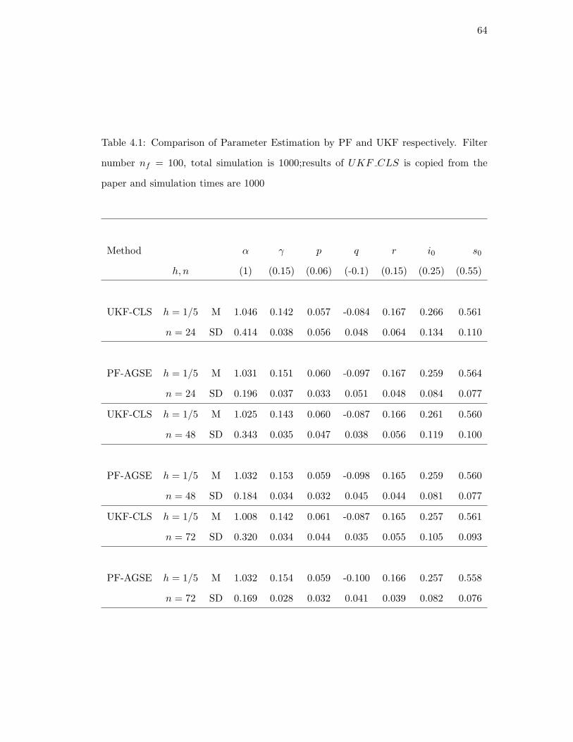
64

Table 4.1: Comparison of Parameter Estimation by PF and UKF respectively. Filter

number nf = 100, total simulation is 1000;results of UKF CLS is copied from the

paper and simulation times are 1000

Method α γ p q r i0 s0

h, n (1) (0.15) (0.06) (-0.1) (0.15) (0.25) (0.55)

UKF-CLS h = 1/5 M 1.046 0.142 0.057 -0.084 0.167 0.266 0.561

n = 24 SD 0.414 0.038 0.056 0.048 0.064 0.134 0.110

PF-AGSE h = 1/5 M 1.031 0.151 0.060 -0.097 0.167 0.259 0.564

n = 24 SD 0.196 0.037 0.033 0.051 0.048 0.084 0.077

UKF-CLS h = 1/5 M 1.025 0.143 0.060 -0.087 0.166 0.261 0.560

n = 48 SD 0.343 0.035 0.047 0.038 0.056 0.119 0.100

PF-AGSE h = 1/5 M 1.032 0.153 0.059 -0.098 0.165 0.259 0.560

n = 48 SD 0.184 0.034 0.032 0.045 0.044 0.081 0.077

UKF-CLS h = 1/5 M 1.008 0.142 0.061 -0.087 0.165 0.257 0.561

n = 72 SD 0.320 0.034 0.044 0.035 0.055 0.105 0.093

PF-AGSE h = 1/5 M 1.032 0.154 0.059 -0.100 0.166 0.257 0.558

n = 72 SD 0.169 0.028 0.032 0.041 0.039 0.082 0.076

65

Table 4.2: Comparison of Parameter Estimation by PF and UKF respectively. Filter

number n1 = 100, total simulation is 1000;results of UKF CLS is copied from the

paper and simulation times are 1000

Method α γ p q r i0 s0 k2

h, n (1) (0.15) (0.06) (-0.1) (0.15) (0.25) (0.55) (0.01)

UKF-CLS h = 1/5 M 1.069 0.148 0.056 -0.082 0.173 0.290 0.549 0.011

n = 24 SD 0.388 0.038 0.054 0.046 0.066 0.142 0.119 0.008

PF-AGSE h = 1/5 M 1.032 0.158 0.060 -0.093 0.172 0.272 0.551 0.0036

n = 24 SD 0.204 0.042 0.034 0.048 0.052 0.087 0.083 0.0042

UKF-CLS h = 1/7 M 1.054 0.149 0.057 -0.087 0.170 0.275 0.557 0.011

n = 48 SD 0.338 0.036 0.045 0.037 0.057 0.128 0.106 0.008

PF-AGSE h = 1/7 M 1.022 0.155 0.057 -0.094 0.172 0.264 0.554 0.0061

n = 48 SD 0.191 0.036 0.032 0.041 0.045 0.087 0.082 0.0042

UKF-CLS h = 1/10 M 1.046 0.149 0.059 -0.087 0.170 0.263 0.560 0.012

n = 72 SD 0.325 0.035 0.043 0.034 0.054 0.116 0.094 0.008

PF-AGSE h = 1/10 M 1.009 0.153 0.061 -0.093 0.170 0.256 0.554 0.0066

n = 72 SD 0.187 0.035 0.030 0.037 0.045 0.086 0.080 0.0038

Table 4.3: PF-loglike Estimator of Bartonella Data

α γ p q r i0 s0

PF-GSE 2.350(0.063) 0.087(0.004) 0.425(0.016) 0.175(0.010) 0.825(0.022) 0.328(0.029) 0.484(0.024)

UKF-CLS 2.127(0.485) 0.109(0.018) 0.534(0.149) 0.057(0.048) 0.645(0.137) 0.318(0.113) 0.552(0.103)

66

Chapter 5

Functional Time Series driven by its Feature Process

5.1 Background

The chapter introduces a new, general method via state space model for modeling and

forecasting time series of functions. More specifically, when the underlying continuous,

smooth function is a function of another dynamic process, which can be modeled and

predicted by time series models, we propose a functional time series model driven by

its feature process model(FTS-FP). The structure between observed functional data

and latent process at each time point is determined by known knowledge or by choos-

ing form of best fit function from a pre-specified group of function forms. This model

achieves model reduction and provides a coherent description of the dynamic system

and an efficient way to do prediction. When the functional time series are density func-

tions, a corresponding model called distributional time series driven by feature process

model(DTS-FP) is proposed. These two models are applied to model the dynamic

of 17-dimension yield curve for U.S. Treasure Bond and that of cross-sectional stock

returns.

The first application uses the FTS-FPM to model and forcast 17-dimensional yield

curves for U.S. Treasury bonds. Denoting the set of yields as y(τ), where τ denotes

maturity, Nelson and Siegel (1987) express a large set of yields of various maturities as

a function of three unobserved factors as follows.

y(τ) = β0 + β1(1− e−λτ

λτ) + β2(

1− e−λτ

λτ− e−λτ ), (5.1)

where β1,β2,β3 are time-varying level,slope and curvature respectively. Diebold and Li

67

(2006) shows that this representation can be interpreted as a latent factor model and

uses three AR(1) model to model the dynamic change of them:

βi,t = ci + γiβi−1,t, i = 0, 1, 2 (5.2)

Their approach shows encouraging predication results, especially in long prediction

horizons. Further, Diebold et al. (2004) formatted this two-step approach in a state-

space model (DNS-AR) by taking Xt = (β0,t, β1,t, β2,t):

(Xt − µ) = F (Xt−1 − µ) + ηt

yt = GXt + εt

ηt

εt

∼ WN(0

0

,

Q 0

0 H

).

As noted in their paper, putting Nelson-Siegel form into a state-space representation

has several advantages. First, Kalman filter can be easily applied to get MLE estima-

tors and optimal filtered and smoothed underlying factors. Also, one-step Kalman filter

simultaneously estimates all parameters, hence preferable over two-step approach. Fur-

ther, the state-space representation allows for extensions, such as heteroskedasticity and

heavy-tailed measurement errors. Bowsher and Meeks (2008) proposes functional signal

plus noise(FSN) model to forcast the yield curve. It models the underlying, continuous

economic function (or ‘signal’) as a natural cubic spline whose dynamic evolution is

driven by a cointegrated vector autoregression for the ordinates (or ’y-values’) at the

knots of the spline. This also results in a linear, state space model. Both of their

endeavors are special cases of our FTS-FPM. Motivated by the empirical observation of

different transition dynamics conditioned on different former shapes, here we take the

approach of Diebold et al. (2004) and propose a FTS-FP model incorporating the shape

of the yield curve to model the driving factors. It is found that this model provides

better fit to the data, especially when the former yield curve is inverted type. Due to

limited inverted type in the data set, parameter estimation for dynamic of the inverted

type yield curve transition is not stable and a cross-validation type of data split is used

to measure the predictive power. We find when the training and testing data set have

68

reasonable number of the inverted types, the proposed model is superior over almost

all maturities compared to DNS-AR or random walk.

The second application concerns the dynamic of the return distribution of all secu-

rities in the market. Represented by Capital Asset Pricing model (Fama and French

(1992)), researchers and practicers have been focusing on expected equity return of a

specific security. Not enough attention has been paid on the property of the cross-

sectional distribution, i.e. how the return distribution of all securities at the market

change over time. The noted stock indices (e.g. Dow Jones, S&P500) are essentially

statistics calculated out of that distribution. The cross-sectional distributions provide

a more comprehensive picture of the market. Also, with the increasing popularity of

ETF, cross-sectional return distribution of different sectors is able to provide impor-

tant information on the dynamic of stock returns out of a specific sector, e.g., expected

return, risk etc.

Lillo and Mantegna (1999) investigates the statistical properties of a ensemble of

daily stock returns by extracting its first four central moments and characterizing them

by their probability density function and temporal correlation properties. Cont (2001)

presentes a set of stylized empirical facts on the statistical property of return common

in most financial markets, which includes asymmetry and heavy tail. It is pointed

out in his paper that ”in order for a parametric model to successfully reproduce all

the above properties of the marginal distributions, it must have at least four parame-

ters: a location parameter, a scale (volatility) parameter, a parameter describing the

decay of the tails and eventually an asymmetry parameter allowing the left and right

tails to have different behaviors”. Here we use the skewed t-distribution to account

for the empirically observed fat tail and asymmetry in our empirical cross-sectional

stock return. The Skew-t distribution has been proposed by different researchers from

different perspective. Jones and Faddy (2003) proposes a tractable skew t-distribution

and the likelihood inference for the parameters of the skew t-distribution. Azzalini

69

and Capitanio (1999) proposes an approach to construct a skew-t distribution from a

skew-normal distribution. Fernandez and Steel (1996) presentes a general method to

transform any symmetric and unimode distribution to a skewed distribution. Here we

use the skew t-distribution version of Fernandez and Steel (1996). However, it is found

in our analysis that parameters fitted by the latter two approaches are equivalent ex-

cept that skewness parameter out of Azzalini and Capitanio (1999) approach is about

4 times that out of Fernandez and Steel (1996).

Therefore, under the framework of distributional time series, we proceed to study the

cross-sectional distribution of stock returns by fitting a skew t-distribution. We then

proceed to explore the dynamic of the underlying distributional parameter. Vector

moving average model (VMA) is found to be an appropriate model for the dynamic

and is used to predict one-step ahead cross-sectional return distribution. Compared to

simple mean and random walk model, our DTS-FP model shows superior performance

in predicting both the underlying distributional parameter and the whole distribution.

This chapter is organized as follows. First we set up the general framework for func-

tional time series and introduces the class of FTS-FP models and DTS-FP models. The

estimation, prediction and model building procedure are described in section 2. Sec-

tion 3 presents the specification and estimation of FTS-FP model for zero-coupon yield

curve and compares their out of sample performance with simpler models using mean

square measurement error (MSME)-based criteria. The application of DTS-FP model

on cross-sectional distribution prediction is presented in section 4. Summarization of

the results and discussion are in the last section.

5.2 Model Set-up

Let (M,Λ) ba a measurable metric space. Often Λ is taken as the Borel σ-algebra

generated by all the open sets in M. For any t ∈ Z ≡ · · · ,−1, 0, 1, · · · , if Yt ∈ M

is a Λ-measurable random functional, we call Yt : t ∈ Z a functional time series

70

(FTS). When M = R, Yt is a conventional real-valued time series. For a curve time

series, M may consist of all (continuous) functions defined on an interval [a, b]. If M

consists of probability density (distribution) functions in certain space, then Yt forms a

distributional time series (DTS). Here we consider two special types of functional time

series and proposes two models accordingly.

5.2.1 FTS Driven by Finite Dimensional Dynamic Processes

A functional time series Yt(·) is said to be driven by a dynamic process Xt if, for

any fixed t , the function Yt(·), defined on Ω, can be written as

Yt(s) = gt(s;Xt) + εt(s), s ∈ Ω (5.3)

where the function gt(·) is known up to Xt. Here εt(s) is a noise process defined on Ω

with E(εt(s)) = 0 for all s ∈ Ω. We also assume εt1(s1) and εt2(s2) are independent for

t1 = t2. In this case, the dependency between Yt and its previous record is completely

characterized by the parameter process Xt and the noise process εt. We call Xt

the driving process or the feature process. In most of the applications, Yt(·) is only

observed at a finite number of observations. In the following we assume that for each

time t, a set of observations Yt = Yt(sti), i = 1, · · · ,mt is available, satisfying

Yt(sti) = gt(sti;Xt) + εt(sti).

When functional time series Yt is driven by a finite dimensional process Xt, it

in fact assumes a hierarchical model with functional observations and dynamic laten

processes. It can be written as a generalized state space model:

Yt(sti) = gt(sti;Xt) + εt(sti), i = 1, · · · ,mt,

Xt = f(Xt−1, · · · ,Xt−p, et, ..., et−q, θ),

(5.4)

where f(·) is a known function with unknown parameters θ and et is a sequence of

scalar or vector white noises. For example, one can use a vector ARMA(p,q) model for

the factor.

71

In real applications, there might be some prior information on how observation

equation is structured but the time series model for Xt is not given. In such cases, one

can first use the observation (Yt(sti), sti), i = 1, · · · ,mt at time t to estimate Xt,

as a linear/non-linear regression problem. Using time series Xt, then one can specify

one or several potential candidate models and estimate the corresponding parameters.

Model selection, goodness-of-fit or prediction performance evaluation procedures can

be carried out to identify the most appropriate model. In case estimation of Xt in the

first step might not be accurate, joint estimation and model evaluation for the whole

state space model, with candidates models for Xt, can also be considered.

An naive predictor of Yt+d(·) is the plug-in predictor Yt+d(s) = g(s, Xt+d),where

Xt+d is the prediction of Xt+d at time t, under model (5.4) and the estimated param-

eter θ. For Gaussian state space model,under squared error loss, such an estimator is

optimal.

5.2.2 DTS Driven by Finite Dynamic Processes

Let πt be a sequence of distributions, indexed by time t. The objective is to understand

the distribution dependency between time and make use of that to predict future distri-

bution. Assume at time t we observe independent observations Yt,i ∼ πt, i = 1, ...,mt.

Similar to the case of curve time series, if the distribution πt belongs to a parametric

family πt(y) = π(y;Xt) and Xt follows a dynamic process, then we call the distribu-

tional time series πt as being driven by a dynamic process.

The distributional time series model representation, parallel to that of functional

time series is:

Yt,i ∼ π(Xt), i = 1, · · · ,mt,

Xt = f(Xt−1, · · · ,Xt−p, et, ..., et−q, θ),

(5.5)

where f(·) presents a time series model with unknown parameters θ and et is a scalar

or vector white noise series. Such problems can be seen in many applications. For

example, the simplest version of the popular stochastic volatility model in finance takes

72

the form Yt ∼ N(0, h2t ), where ln(h2t ) = θ0 + θ1 ln(h2t−1) + et. It is a special case of our

model, with one observation per time period. Another example is when an underlying

time series Yt is observed multiple times with noise, e.g. in the form Yt,i ∼ N(Yt, σ2t ). In

this case, we also have the flexibility to add certain structure for σ2t as in the stochastic

volatility models or heteroscadicity in the form σ2t = σ2Y 2

t .

5.3 Application: Modeling and Forecasting Treasury Yield Curve

The first application uses the same dataset as in Diebold-Li, which are end-of-month

price quotes (bid-ask average) for U.S. Treasuries, from January 1985 through June

2000. Yields are linearly interpolated nearby maturities to pool into fixed maturities of

3, 6, 9, 12, 15, 18, 21, 24, 30, 36, 48, 60, 72, 84, 96, 108, and 120 months.

5.3.1 Yield Curve Shape

It is widely observed that yield curve exhibits different shapes, which can be roughly

partitioned into four types: Nominal (Increasing), Inverted (Decreasing), Humped (Up-

Down, Down-Up). To quantify this charicteristics, one natural way is making use of

the Nelson-Siegel (NS) Curve fitted to each set of yield curve data. Based on the curve

form (5.1) and fitted parameters, one can then take derivatives and further classify

curve shape by some naive method, such as the one below:

S(Yt) =

1(Increasing) if min(NS′(Yt)) > 0

2(Decreasing) if max(NS′(Yt)) < 0

3(Down-Up) if min(NS′(Yt)) < 0,max(NS′(Yt)) > 0

and NS−1(max(NS(Yt))) < NS−1(min(NS(Yt)))

4(Up-Down) otherwise

where NS′(Yt) is the derivative of NS curve at all maturities and NS−1(·) is the inverse

function of NS curve.

The above definition makes use of derivatives and locations of extreme value of

NS curve to partition shapes. NS curve is weighted for maturities from 7 to 96 in all

73

the following analysis to avoid subtle shape changes in short term maturity. The first

nine yield curves classified as Up-Down (Figure 5.1) show that such definition gives

appropriate shape classification. Empirical shape transition matrix (Table 5.1), as well

as the mean of yield curve plot colored by different shapes (Figure 5.2), indicates that

over the years, normal shapes dominate curve shape and shapes are usually clustered.

0 20 60 100

6.06.3

6.6

tau

x[k, −

1]

0 20 60 100

6.56.7

6.9

taux[k

, −1]

0 20 60 100

6.40

6.55

6.70

tau

x[k, −

1]

0 20 60 100

7.48.0

8.6

tau

x[k, −

1]

0 20 60 100

7.68.0

8.4

tau

x[k, −

1]

0 20 60 100

6.57.5

tau

x[k, −

1]

0 20 60 100

6.97.1

tau

x[k, −

1]

0 20 60 100

5.56.5

7.5

tau

x[k, −

1]

0 20 60 1006.5

7.07.5

tau

x[k, −

1]

Figure 5.1: The first nine yield curve classified as Up-Down. The circles are the observed

yield while the line is the fitted Nelson-Sigel curve

Table 5.1: Empirical Shape Transition Matrix

Former / Current 1 2 3 4 Total

1 223 3 6 14 246

2 5 23 4 4 36

3 7 2 8 2 20

4 10 8 2 26 46

74

0 50 100 150 200 250 300 350

46

810

1214

Mean of yield curve

Index

mea

nyie

ld

NormalInvertedDown−UpUp−Down

1994/01

Figure 5.2: Time series of the mean of the yield curve fitted by NS curve. Different

shapes are denoted by different colors

5.3.2 FTS-FP for Modeling Yield Curve

The rational for our proposed model is the evolution of underlying factors, hence the

whole yield curve, might be depending on the shape of former yield curve. This is

empirically validated by Figure 5.3 which plots βi,t vs βi,t−1 with the shapes of yield

curve at time t-1 specified by different colors. It suggests a multi-regime AR model

might be a better fit for the feature process.

Motivated by the empirical observation that different transition dynamics depends

on different prior shapes, we propose a FTS-FP model. It is documented that AR model

is preferred over VAR as the transition equation (confirmed by our results), hence we

set the coefficient matrix FIt to be diagonal to simplify the model. We also assume

75

that Q is non-diagonal and H is diagonal.

Xt = µIt0 + FItXt−1 + ηItt

Yt = GXt + εt

It =

2(Inverted) if S(Yt)) = 2

1(Non-Inverted) otherwise

ηItt

εt

∼ N(0

0

,

QIt 0

0 H

)

(5.6)

It is obvious that our model is a generalization of Diebold’s model, hence provides

more flexibility in capturing certain characteristics in the data. Index in this paticular

setting is chosen to be It = S(Yt)) (i.e., the shape of the former yield curve). It can

also be replaced by other choices. Also, some elements of µt and FIt could be the same,

allowing for the same dynamic change in certain βi. For example, level change might be

indifferent to the shape while curvature dynamic is more sensitive to the former shape.

5.3.3 Model Estimation

For a given parameter configuration, we use the Kalman filter to compute the likelihood

and find MLE. We initialize the Kalman filter using the unconditional mean (zero) and

unconditional covariance matrix of the state vector in the one regime case. We maximize

the likelihood by L-BFGS-B method in R function ”optim”, with a convergence criterion

of 10−6 for the change in the norm of the parameter vector from one iteration to the

next. To ensure the variance-covariance matrix is positive, we estimate the Choleski

decomposition of it. We use the same startup parameter values as in Diebold and

Li (2006) (i.e., using the Diebold-Li two-step method to obtain the initial transition

equation matrix, initializing all variances at 1.0, and initializing unknown parameters

at the values given in Diebold et al. (2004)).

The estimation of model (5.6) is shown in Table 5.2. The transition dynamic for

the non-inverted type shows strong momentum in all three factors (level, slope and

curvature) and is similar to the estimation when no inverted type is separated out.

76

When the former type is inverted yield curve, expected level of the next yield curve

would be 0.16 less. It corresponds to the fact that when in a recession (as companied by

the prior inverted yield curve), the expectation for the long-term yield would be low.

On the contrary, the slope and curvature would have a big change compared to the

former inverted yield curve. This reflects the empirically observed fact that unlike the

stable economical condition, which is always expected to be followed by another stable

period, there could be a couple of possibilities following a recession period. In terms

of the yield curve, instead of always being followed by another inverted yield curve,

other three shapes of yield curve (increasing or humped) are also expected to appear.

The estimation of the dynamic change following the inverted yield curve therefore can

be seen as an averaged expectation of all possibilities. Such uncertainty as well as the

small size of observed inverted yield curve account for the large standard deviation in

the inverted type estimations.

5.3.4 Model Comparison

We then compares the measurement and forecast performance of the proposed model

(AR-2regime) with that from three rival models: a random walk for the yield curve

(RW), Diebold et al. (2004) dynamic Nelson-Siegel model with diagonal and non-

diagonal transition matrix (henceforth DNS-AR and DNS-VAR). To make the result

comparable, we choose the training data set to be the monthly yield curve data from

January 1985 to December 1993.

Bowsher and Meeks (2008) used the percentage increase in mean squared measure-

ment error(MSME) relative to the RW as the evaluation criterion its invariant property.

We adopt the same criterion here and plot them by maturity in Figure 5.4, which shows

MSME from different models. Inspection of the above figure reveals that our proposed

model provides better fit the data, especially for the inverted shape.

77

Table 5.2: Parameter estimation for model (5.6) fitted on monthly yield curve data,

the standard error is in the right lower corner

shape parameter β0 β1 β2

1(Normal) µ0 0.25(0.10) −0.02(0.06) −0.066(0.05)

2(Inverted) µ0 −0.16(0.28) 1.00(0.48) −0.11(0.31)

1(Normal) diag(A) 0.97(0.01) 0.98(0.02) 0.89(0.03)

2(Inverted) diag(A) 1.03(0.03) 0.48(0.19) 0.46(0.19)

Q1 β0 β1 β2

β0 0.10 -0.01 0.02

β1 -0.01 0.33 -0.02

β2 0.02 -0.02 0.59

Q2 β0 β1 β2

β0 0.12 0.03 0.01

β1 0.03 1.28 0.04

β2 0.01 0.04 3.12

Because of the limited number of testing data in inverted shape, it is hard to com-

pare forecasts based on that. It is found in former research papers and here that the

testing period we use here has a rather stationary dynamic that favors DNS-AR model.

Different model captures different characteristics of yield curve, hence may have differ-

ent prediction performances as dynamics of the prediction period varies. In our case,

this depends on how different shapes are distributed. To explore the impact of pre-

diction period and shape distribution on model comparison, we run a cross-validation

type of experiment on the yield curve data set. It is done as follows:

• Evenly split the data into K-fold, by splitting the time line into I time period

(TP),i.e. [ti−1, ti)Ii=1 ;

For i=1, 2, · · · , I:

78

• Take out y[ti−1,ti) as the testing data set and the other data in the whole dataset

as the training set, denoted as y[tj−1,tj)−i.

• for each candidate model, find the optimal parameter estimators based on y[tj−1,tj)−i,

hold them constant and get the prediction value on y[ti−1,ti).

Table 5.3: Number of inverted shapes and estimated parameters in different training

data set

TP1 TP2 TP3 TP4

Inverted 8 23 1 1

Slope Intercept 0.94 -0.17 -0.02 -0.02

Slope AR 0.54 0.88 0.92 0.90

Curvature Intercept -0.10 0.03 -0.24 -0.10

Curvature AR 0.44 0.96 0.62 0.75

There are several observations from this experiment:1) High AR coefficients of level,

slope and curvature over all time periods indicate strong momentum for the non-inverted

shape transition. 2) For inverted type, due to limited observations, parameter estima-

tion seems to unstable and depends on the training dataset. Prediction is also greatly

impacted by number of inverted types in the testing data. An interesting split to is TP1,

as now there is enough inverted type in both training (25) and testing (8). Seen from

the first figure of MSME comparison graph, our proposed model has better prediction

in almost all maturities for this split.

5.4 Application: Cross-sectional stock return distributions

5.4.1 Fitting of Skew T-distribution

Data used in this analysis are the daily returns for the 1000 largest capitalization stocks

in the CRSP database from 1991 to 2002. To ensure model stability, two daily returns

with extreme small mean and large variance are removed as outliers.

79

The density function of the skewed-t distribution proposed by Fernandez and Steel

(1996) is:

P (y|µ, σ, ν, λ) =

√

(1− λ)(1 + λ)Γ( ν+1

2)√

νπσ2Γ( ν2)(1 + (y−µ)2(1+λ)

λ2ν(1−λ))− ν+1

2 y ≤ λ√(1− λ)(1 + λ)

Γ( ν+12

)√νπσ2Γ( ν

2)(1 + (y−µ)2(1−λ)

λ2ν(1+λ))− ν+1

2 y > λ,

where µ is the location parameter(−∞ < µ < ∞), σ is scale parameter(σ > 0), λ

is skewness parameter(−1 < λ < 1) and ν is degrees of freedom(ν > 0). There are

several nice properties about this skew-t distribution representation and the skewness

parameter has a very intuitive interpretation. With µ as the unique mode in the

distribution, skewness λ is exactly equal to the measurement of skewness introduced by

Arnold and Groeneveld (1995), (i.e., one minus two times the probability mass to the

left of the mode). When λ = 0, P (y|µ, σ, ν, 0) becomes the symmetric t-distribution

with location and scale parameter (µ, σ) and degrees of freedom ν. λ controls the

allocation of weights to the left and right side of the mode. P (y ≥ µ|µ, σ, ν, λ) = 1+λ2

and P (y < µ|µ, σ, ν, λ) = 1−λ2 . Changing the sign of λ produce a mirror image of the

density function around µ.

The loglikelihood of this skew t-distribution is:

log(L) = N ∗ Const− ν + 1

2

∑yi>µ

ln(1 +(y − µ)2(1− λ)

λ2ν(1 + λ))− ν + 1

2

∑xi≤µ

ln(1 +(y − µ)2(1 + λ)

λ2ν(1− λ))

Const = lnΓ(ν+1

2 )√νπσ2Γ(ν2 )

+1

2ln

(1− λ)(1 + λ)

νπλ2.

L-BFGS-B method in R function ”optim” is used to maximize the likelihood function

to find the MLE of the four parameters. It is very sensitive to the starting value,

therefore different starting values are used to find the global maximum of the likelihood

function. Summary statistics for the MLE of the parameters are presented in Table

5.4. All p-values of the Kolmogorov–Smirnov test are significant small than 0.01, which

indicates the fit of the skew t-distribution on the returns is quite good.

As seen from the time series plots of the parameter estimates in Figure 5.6, a

comprehensive picture about the whole market return can be obtained over the period

80

Table 5.4: Summary statistics of estimated parameters of the skew t-distribution

µ σ λ ν

Mean -0.0011 0.0146 0.0496 3.4021

Stdev 0.0065 0.0051 0.1789 1.0149

Min -0.0436 0.0066 -0.5712 1.4257

Median -0.0008 0.0128 0.0644 3.2229

Max 0.0522 0.0650 0.6404 26.0971

Jan 1,1991 to Dec 31, 2002:

• Location of the return is always very close to 0, though the variation of the

location becomes large in the later period;

• Scale parameter becomes much larger after March 1998.

• Most degrees of freedom are below 5, which suggests a fat tail and necessity of

fitting a fat tail distribution.

• There are approximately three subperiods with different cross-sectional return

behaviors.

”Stable Period”: Before March 1998, the return distribution shows location

around 0, small diversification (scale),and slightly positive skewness.

”Wild Period”: Period between May 1998 and March 2000 has much more

turmoil and right skewness. This reflects the wild stock market before the

dot come bubble burst on March 2000.

”Recovery Period”: With stocks slowly recovering from the bubble burst,

periods after year 2000 sees an upward trend in location and decreased scale

and skewness.

81

5.4.2 DTS-FP for Cross-Sectional Return Distribution

Obviously the dynamic of cross-sectional returns become more volatile after 1998. Be-

fore that the distributional parameters are more stable and predictable. To give an

illustration of the predicative power of our approach, we apply the method only on

period from 1991 to 1998. Any other stable and predictive process can be modeled

similarly. There are total 1769 days of observed cross-sectional returns and we split it

into training and testing dataset: the first 1600 days and the other days left. To ensure

positivity for variance, we model lnσ2 instead of σ2. Also to avoid jumps in degree of

freedom, the continuous transformation of degree of freedom: ζ = Ptν (t < 2) is used to

represent the dynamic of ν, where the probability function is calculated on a standard

t-distribution with degree ν. Similarly, we model ln ζ instead of ζ to ensure positivity

on µ. Slowly lag autocorrelation decaying in the autocorrelation function of both lnσ2t

and ζt suggests taking difference on these two time series, which is also confirmed by

the Augmented Dicky Fuller(ADF) test p-value. Now the task is to find a vector time

series model for the stationary process (µt, lnσ2t

σ2t−1

, ln ζtζt−1

, λt). (Figure 5.7)

The model building procedure is as follows:

1. Find an appropriate ARMA model for each time series separately and get the

residual time series;

2. Check the cross-correlation matrix of the four residual time series;

3. Specify an proper VARMA model based on 1)&2) and do a joint estimation of

the model;

4. Residual diagnostic analysis on the residuals out of the full model, go back to step

3) if any modification on the model is needed.

Following the above procedure, VMA model with only concurrent correlation is appro-

priate for the underlying feature process (µt, lnσ2t

σ2t−1

, ln ζtζt−1

, λt). The joint estimation

82

of all the parameters(with standard deviation in the right lower coner) is:

µt = −0.000860.00011 + 0.130.023a1,t−1 + a1,t,

lnσ2t

σ2t−1

= −0.520.021a2,t−1 − 0.180.024a2,t−2 − 0.120.021a2,t−3 + a2,t,

λt = 0.0590.004 + 0.280.02a3,t−1 + a3,t,

lnζtζt−1

= −0.710.02a4,t−1 − 0.140.02a4,t−2 − 0.080.02a4,t−3 + a4,t,

a1,t

a2,t

a3,t

a4,t

∼ WN

(

0

0

0

0

,

0.00001 0.00008 0.00015 0.00001

0.00008 0.04586 −0.00073 −0.01498

0.00015 −0.00073 0.01973 0.00089

0.00001 −0.01498 0.00089 0.01346

).

The above estimated model further quantifies the dynamic of the underlying distri-

bution parameter for the return distribution:

• Both µt and λt are modeled by MA(1). Location parameter has a mean with

small magnitude but significantly negative while the mean of skewness is signifi-

cantly positive. Both of them are positively correlated with former shocks, which

suggests some momentum property;

• MA(3) is employed to model ∆ lnσt and ∆ ln ζt. Mean of zero indicates no mean

change in lnσt and ln ζt.

• Concurrent correlation matrix of the shocks reveals an interesting things about

the interaction within the parameters to determine the final distribution: positive

correlation between shock of location and that of skewness. This indicates that

the higher the return location, the more positively skewed the whole distribution.

In more practical sense, when the market condition is good, more stocks have

higher than market return and verse vise. It confirms the finding that skewness

parameter has a significant linear relationship with S&P500. Also, it suggests

beta in CAPM for a specific stock might be conditioned on the market condition.

83

5.4.3 Prediction Performance Comparison to Simpler Models

The estimated model is used in predicting the testing data set to assess the predictive

power for the next return distribution. Models to be compared with are the mean model,

i.e. mean of the historical optimal parameter values are used to predict next return

distribution, and the random walk model, i.e. tomorrow’s distribution is predicted by

today’s. Three measurements are used to quantify the prediction performance:

Relative Accuracy Estimator RAE =1

T

T∑t=1

∣∣Xt − Xt

Xt

∣∣,Relative Loglikelihood Accuracy Estimator RLAE =

1

T

T∑t=1

∣∣LLXt− LLXt

LLXt

∣∣,Absolute Error Estimator AEE =

1

T

T∑t=1

|Xt − Xt|,

where Xt is the estimated distributional parameter, Xt is the optimal distributional

parameter fitted from the realized daily returns, and LLXt is the loglikelihood of the

skew t-distribution given the set of parameter Xt.

Table 5.5: Prediction Performance Comparison between different models on the testing

dataRAE AEE

DTS-FPM Mean Model Random Walk DTS-FPM Mean Model Random Walk

Location 0.12 0.28 3.59 0.0044 0.0043 0.065

scale 0.17 0.18 0.21 0.000028 0.000031 0.000034

skewness 0.39 0.18 2.70 0.10 0.11 0.12

df 0.14 0.15 0.18 0.52 0.53 0.65

RLAE 0.042 0.047 0.073

Figure 5.8 compares the series of (µt, σ2t , νt, λt) predicted by DTS-FP model and the

ones fitted from the realized data. Table 5.5 compares the prediction performance under

different models. In terms of both the RAE and AEE criterion for each parameter, VMA

model greatly improves all parameter estimations compared to mean and former model.

This is in accordance with the appropriateness of MA models for (µt, lnσ2t , ln ζt, λt). In

84

predicting the scale parameter, huge improvement is attained with time-varying model

over constant model. This observation agrees with the observed changing volatility

property in financial market. The limited improvement of the likelihood over mean

model might due to the small magnitude of underlying parameters and fitted coefficients

in VMA model, which result small likelihood difference. However, our approach does

improve the prediction power over both mean and former model on the testing data.

5.5 Conclusion

This chapter presents two applications in the analysis of functional time series driven

by its feature process via state space model. This includes two procedures: first find the

underlying feature process and build its transitional relationship, providing the basis

to be converted into a SSM form; Second calibrate the state space model by likelihood

calculated from the filtering scheme.

The first application analyzes the U.S. treasury yield curve from January 1985

through June 2000. By NS curve, the 17 dimensional time series could be represented

well by the underlying feature process: level, slope and curvature. The feature process

is further modeled as a two-regime AR process. The regime is characterized by the

shape of the former yield curve. This process, together with the NS curve, constitute

the SSM. Kalman Filter is utilized to get the likelihood and MLE is obtained. It is

found that this model provides better fit to the data, especially when the former yield

curve is the inverted type. Due to limited inverted type in the data set, parameter

estimation for dynamic of inverted type yield curve transition is not stable and a cross-

validation type of data splits is used to measure the predictive power. We find that

when both the training and testing data set have reasonable number of inverted type,

the proposed model is superior over almost all maturities comparing to DNS-AR or

random walk.

The second application applies the framework to the daily returns distribution of

85

the 1000 largest capitalization stocks in the CRSP database from 1991 to 2002. The

target daily return distribution could be well fitted by a novel skew-t distribution.

Characterized by the skew-t distribution, the feature processes are naturally taken

as the parameters of the distribution: location, scale, skewness and kurtosis. Time

series of the estimated feature process clearly captures the dynamic of the market and

clearly exhibits three different subperiods: ”stable period”, ”wild period” and ”recovery

period”. A vector moving average model is proposed and used to predict one-step

ahead cross-sectional return distribution. Compared to simple mean and random walk

model, our DTS-DP model shows superior prediction performances in both underlying

distribution parameter prediction and the whole distribution prediction.

86

4 6 8 10 12 14

46

810

1214

belta(t−1)

belta(

t)NormalInvertedDown−UpUp−DownTestData

belta0

−6 −4 −2 0 2 4 6

−6−4

−20

24

6

belta(t−1)

belta(

t)

NormalInvertedDown−UpUp−DownTestData

belta1

−6 −4 −2 0 2 4 6

−6−4

−20

24

6

at_est[3, which(index2 == 1)]

at_est

[3, wh

ich(in

dex2

== 1)

+ 1]

NormalInvertedDown−UpUp−DownTestData

belta2

Figure 5.3: βi,t vs βi,t−1, with the shapes of yield curve at previous time specified by

different colors. Here β0, β1, β2 are the level slope and curvature of the yield curve.

87

0 20 40 60 80 100 120

−0.3

−0.2

−0.1

0.0

0.1

0.2

0.3

tau

Rela

tive

MSF

E im

prov

emen

t ove

r Ran

dom

Wal

k

ARVARAR_2 regime

0 20 40 60 80 100 120

−0.3

−0.2

−0.1

0.0

0.1

0.2

0.3

tau

Rela

tive

MSF

E im

prov

emen

t ove

r Ran

dom

Wal

k

ARVARAR_2 regime

0 20 40 60 80 100 120

−0.3

−0.2

−0.1

0.0

0.1

0.2

0.3

tau

Rela

tive

MSF

E im

prov

emen

t ove

r Ran

dom

Wal

k

ARVARAR_2 regime

Figure 5.4: In the training data set, comparison of different models on the percentage

increase in MSME relative to the RW

0 20 40 60 80 100 120

−0.6

0.0

0.4

Time Period 1

tau

Rela

tive

MSF

E im

prov

emen

t

ARAR_2 regime

0 20 40 60 80 100 120

−0.6

0.0

0.4

Time Period 2

tau

Rela

tive

MSF

E im

prov

emen

t

ARAR_2 regime

0 20 40 60 80 100 120

−0.5

0.5

1.5

Time Period 3

tau

Rela

tive

MSF

E im

prov

emen

t

ARAR_2 regime

0 20 40 60 80 100 120

−0.6

0.0

0.4

Time Period 4

tau

Rela

tive

MSF

E im

prov

emen

t

ARAR_2 regime

Figure 5.5: In the testing data set, comparison of different models on the percentage

increase in MSME relative to the RW on the first four time period

88

−0.04−0.020.000.020.04

loca

tio

n

19

92

19

94

19

96

19

98

20

00

20

02

0.010.020.030.040.050.06

scal

e

19

92

19

94

19

96

19

98

20

00

20

02

−0.6−0.20.00.20.40.6

skew

nes

s

19

92

19

94

19

96

19

98

20

00

20

02

510152025

df

19

92

19

94

19

96

19

98

20

00

20

02

Figure 5.6: Distributional parameters (µ, σ, ν, λ) estimated for the period Jan 1,1991

to Dec 31, 2002. Two vertical lines, drawn on date May 2,1998 and March 2,2000

partitions the dynamic of the market into three different subperiods: ”stable period”,

”wild period” and ”recovery period”.

89

05

00

10

00

15

00

−0.020.000.010.02

loca

tio

n

Ind

ex

05

00

10

00

15

00

−1.0−0.50.00.51.01.5

Dif

f(lo

g(s

cale

))

Ind

ex

05

00

10

00

15

00

−0.4−0.20.00.20.4

skew

nes

s

Ind

ex

05

00

10

00

15

00

−0.6−0.20.20.40.6

Dif

f(Tr

ansf

orm

(df)

)

Ind

ex

Figure 5.7: Fitted distributional parameters after transformation (µt, σ2t , ζt, λt) over the

period Jan 1,1991 to Dec 31, 1998.

90

05

01

00

15

0

−0.015−0.0050.005

NA

Ind

ex

05

01

00

15

0

0.000100.000200.000300.00040

NA

Ind

ex

05

01

00

15

0

−0.3−0.10.10.20.30.4

NA

Ind

ex

05

01

00

15

0

3456

NA

Ind

ex

Figure 5.8: Predicted values for µt(lower left), σ2t (upper left), νt(upper right), λt(lower right)

from different models over the testing period. The circles are the fitted parameters

based on realized daily returns, the red lines connects the predicted parameters by

DTS-FP model and the green line is the mean value of each parameter over the

training time period.

91

Bibliography

Ahn, W. and Chan, K. (2011). Approximate conditional least square estimation of a

nonlinear state-space model via unscented kalman filter, Technical report.

Akaike, H. (1973). Information theory and an extension of the maximum likelihood prin-

ciple, Second International Symposium on Information Theory (Tsahkadsor, 1971),

Akademiai Kiado, Budapest, pp. 267–281.

Akaike, H. (1974). A new look at the statistical model identification, IEEE Trans, on

Automatic Control AC 19: 716–723.

Anderson, R. (1991). Infectious diseases of humans: Dynamics and control, Oxford

University Press, Oxford.

Anderson, R. M. and May, R. M. (1992). Infectious Diseases of Humans: Dynamics

and Control, new edn, Oxford University Press, USA.

Azzalini, A. and Capitanio, A. (1999). Statistical applications of the multivariate skew

normal distribution, Journal of the Royal Statistical Society: Series B (Statistical

Methodology) 61(3): 579–602.

Bengtsson, T. and Cavanaugh, J. E. (2006). An improved Akaike information criterion

for state-space model selection, Computational Statistics & Data Analysis 50: 2635–

2654.

Biegler, L. T., Damiano, J. J. and Blau, G. E. (1986). Nonlinear parameter estimation:

A case study comparison, AIChE Journal 32(1): 29–45.

Boor, C. D. (1972). A practical guide to splines.

92

Bowsher, C. G. and Meeks, R. (2008). The dynamics of economic functions: Modelling

and forecasting the yield curve, Economics Papers 2008-W05, Economics Group,

Nuffield College, University of Oxford.

Boyce, W. and DiPrima, R. (2004). Elementary differential equations and boundary

value problems, 8th edn, Wiley New York.

Broyden, C. G. (1970). The convergence of a class of double-rank minimization algo-

rithms: the new algorithm.

Callaway, D. S. and Perelson, A. S. (2002). HIV-1 infection and low steady state viral

loads, Bulletin of Mathematical Biology 64: 29–64.

Cont, R. (2001). Empirical properties of asset returns: stylized facts and statistical

issues, Quantitative Finance 1: 223–236.

Denham, W. F. and Pines, S. (1966). Sequential estimation when measurement non-

linearity is comparable to measurement error, AIAA journal 4: 1071–1076.

Diebold, F. and Li, C. (2006). Forecasting the term structure of government bond

yields, Journal of Econometrics 130(2): 337–364.

Diebold, F., Rudebusch, G. and Aruoba, S. B. (2004). The macroeconomy and the yield

curve: A dynamic latent factor approach, NBER Working Papers 10616, National

Bureau of Economic Research, Inc.

Diekmann, O. and Heesterbeek, J. A. P. (2000). Mathematical Epidemiology of Infec-

tious Diseases: Model Building, Analysis and Interpretation, 1 edn, Wiley.

Doucet, A., de Freitas, N. and Gordon, N. (eds) (2001). Sequential Monte Carlo Methods

in Practice, Statistics for Engineering and Information Science, Springer-Verlag, New

York.

93

Doucet, A. and Tadic, V. B. (2003). Parameter estimation in general state-space models

using particle methods, Annals of the Institute of Statistical Mathematics 55(2): 409–

422.

Durbin, J. and Koopman, S. J. (2000). Time series analysis of non-Gaussian obser-

vations based on state space models from both classical and Bayesian perspectives,

Journal of the Royal Statistical Society, Series B 62: 3–56.

Durbin, J. and Koopman, S. J. (2001). Time Series Analysis by State Space Methods,

Oxford University Press.

Durham, G. B. and Gallant, A. R. (2001). Numerical techniques for maximum likelihood

estimation of continuous-time diffusion processes, JOURNAL OF BUSINESS AND

ECONOMIC STATISTICS 20: 297–338.

Fama, E. F. and French, K. (1992). The cross-section of expected stock returns, Journal

of Finance 47(2): 427–65.

Fearnhead., P. (1998). Sequential Monte Carlo methods in filter theory, PhD thesis,

University of Oxford.

Fernandez, C. and Steel, M. (1996). On bayesian modelling of fat tails and skewness,

Technical report.

Freed, A. D. and Walker, K. P. (1991). From differential to difference equations for first

order odes, Technical report.

Hannan, E. J. and Quinn, B. G. (1979). The determination of the order of an autore-

gression, Journal of the Royal Statistical Society, Series B 41: 190–195.

Harvey, A. (1989). Forecasting, Structural Time Series Models and the Kalman Filter,

Cambridge University Press, Cambridge.

94

Hethcote, H. W. (2000). The mathematics of infectious diseases, SIAM Review 42: 599–

653.

Ho, D., Neumann, A., Perelson, A., Chen, W., Leonard, J. and Markowitz, M. (1995).

Rapid turnover of plasma virions and CD4 lymphocytes in HIV-1 infection, Nature

373: 123–126.

Hurvich, C. and Tsai, C. (1989). Regression and time series model selection in small

samples, Biometrika 76: 297–307.

Jones, M. C. and Faddy, M. J. (2003). A skew extension of the t-distribution, with

applications, Journal Of The Royal Statistical Society Series B 65(1): 159–174.

Julier, S. J. (1997). New extension of the kalman filter to nonlinear systems, Proceedings

of SPIE 3(3): 182–193.

Julier, S. J. and Industries, I. (2002). The scaled unscented transformation, in Proc.

IEEE Amer. Control Conf, pp. 4555–4559.

Julier, S. and Uhlmann, J. (2004). Unscented filtering and nonlinear estimation, Pro-

ceedings of the IEEE 92(3): 401–422.

Kalman, R. E. (1960). A new approach to linear filtering and prediction problems,

Trans. ASME, Journal of Basic Engineering 82: 35–45.

Kermack, W. O. and McKendrick, A. G. (1927). Contributions to the mathematical

theory of epidemics, part i., Proc Roy Soc London A115: 700–721.

Kitagawa, G. (1996). Monte Carlo filter and smoother for non-Gaussian nonlinear state

space models, Journal of Computational and Graphical Statistics 5: 1–25.

Kitagawa, G. (1998). A self-organizing state-space model, Journal of the American

Statistical Association 93(443): 1203C1215.

95

Kloeden, P. E. and Platen, E. (1992). Numerical solution of stochastic differential

equations, Springer-Verlag, Berlin ; New York :.

Kong, A., Liu, J. and Wong, W. (1994). Sequential imputations and Bayesian missing

data problems, J. Amer. Statist. Assoc 89: 278–288.

Li, Z., O. M. and Prvan, T. (2005). Parameter estimation in ordinary differential

equations, IMA Journal of Numerical Analysis 25: 264C285.

Liang, H., Miao, H. and Wu, H. (2010). Estimation of constant and time-varying

dynamic parameters of HIV infection in a nonlinear differential equation model, The

Annals of Applied Statistics 4: 460–483.

Liang, H. and Wu, H. (2008a). Parameter estimation for differential equation models us-

ing a framework of measurement error in regression models, Journal of the American

Statistical Association 103(484): 1570–1583.

Liang, H. and Wu, H. (2008b). Parameter estimation for differential equation mod-

els using a framework of measurement error in regression models, Journal of the

American Statistical Association 103: 1570–1583.

Lillo, F. and Mantegna, R. N. (1999). Statistical properties of statistical ensembles of

stock returns, Quantitative finance papers, arXiv.org.

Liu, D., Lu, T., Niu, X. F. and Wu, H. (2010). Mixed-effects state-space models for

analysis of longitudinal dynamic systems, Biometrics p. in press.

Liu, J. and Chen, R. (1995). Blind deconvolution via sequential imputations, Journal

of the American Statistical Association 90: 567–576.

Liu, J. and Chen, R. (1998). Sequential Monte Carlo methods for dynamic systems,

Journal of the American Statistical Association 93: 1032–1044.

96

Liu, J. and West, M. (2001). Combined parameter and state estimation in simulation-

based filtering, in A. Doucet, J. F. G. de Freitas and N. J. Gordon (eds), Sequential

Monte Carlo in Practice, Springer-Verlag, New York.

Liu, L.-M., Bhattacharyya, S., Sclove, S., Chen, R. and Lattyak, W. (2001). Data

mining on time series: an illustration using fast-food restaurant franchise data, Com-

putational Statistics and Data Analysis .

Merrill, S. (1987). AIDS: background and the dynamics of the decline of immunocom-

petence, Addison-Wesley, Reading, MA, chapter Theoretical Immunology, part II,

pp. 59–75.

Mittler, J. (1997). Dynamics of HIV-1-infected cell turnover evaluated using mathe-

matical models. international workshop on HIV drug resistance, treatment strategies

and eradication. Abstract 101. Antiviral Therapy.

Nash, J. (2010). Tutorial: Optimization and related nonlinear modelling computations

in r, http://user2010.org/tutorials/Nash.pdf .

Nelson, C. R. and Siegel, A. F. (1987). Parsimonious modeling of yield curves, Journal

of Business 60(4): 473–89.

Nowak, M. A. and May, R. M. (2000). Virus Dynamics: Mathematical Principles of

Immunology and Virology, Oxford University Press, Oxford.

Olsson, J. and Ryden, T. (2008). Asymptotic properties of particle filter-based max-

imum likelihood estimators for state space models, Stochastic Processes and their

Applications 118: 649–680.

Parlett, B. N. (1976). A recurrence among the elements of functions of triangular

matrices, Linear Algebra and its Applications 14(2): 117 – 121.

97

Pedersen, A. R. (1995). A New Approach to Maximum Likelihood Estimation for

Stochastic Differential Equations Based on Discrete Observations , Scandinavian

Journal of Statistics 22(1): 55–71.

Perelson, A., Essunger, P., Cao, Y., Vesanen, M.m Hurley, A., Saksela, K., Markowitz,

M., and Ho, D. (1997). Decay characteristics of HIV-1-infected compartments during

combination therapy, Nature 387: 188–191.

Perelson, A., Neumann, A., Markowitz, M., Leonard, J. and Ho, D. (1996). HIV-1

dynamics in vivo: virion clearance rate, infected cell life-span and viral generation

time, Science 271: 1582–1586.

Perelson, A. S., Kirschner, D. E. and Boer, R. D. (1993). Dynamics of HIV infection

of CD4+ T cells, Mathematical Biosciences 114: 81 – 125.

Perelson, A. S. and Nelson, P. W. (1999). Mathematical analysis of HIV-1 dynamics in

vivo, SIAM Review 41: 3–44.

Pitt, M. K. (2002). Smooth particle filters for likelihood evaluation and maximisation,

Technical report.

Poyiadjis, G., Doucet, A. and Singh, S. (2005). Particle methods for optimal filter

derivative: application to parameter estimation, Acoustics, Speech, and Signal Pro-

cessing, 2005. Proceedings. (ICASSP ’05). IEEE International Conference on, Vol. 5,

pp. v/925 – v/928 Vol. 5.

Ramsay, J. O., Hooker, G., Campbell, D., Cao, J. and Ramsay, J. O. (1996). Principal

differential analysis: Data reduction by differential operators, Journal of the Royal

Statistical Society, Series B .

Ramsay, J. O., Hooker, G., Campbell, D., Cao, J. and Ramsay, J. O. (2007). Parameter

estimation for differential equations: A generalized smoothing approach, Journal of

the Royal Statistical Society, Series B .

98

Rimmer, D., Doucet, A. and Fitzgerald, W. (2005). Particle filters for stochastic dif-

ferential equations of nonlinear diffusions, Technical report, University of Cambridge,

Department of Engineering, Cambridge, UK.

Schwarz, G. (1978). Estimating the dimension of a model, The Annals of Statistics

6: 461–464.

Silverman, B. W. (1986). Density estimation: for statistics and data analysis, London.

Sorenson, H. W. (1988). Bayesian Analysis of Time Series and Dynamic Models, j. c.

spall edn, Marcel Dekker.

Sorenson, H. W. and Stubberud, A. R. (1968a). Recursive fltering for systems with

small but nonnegligible nonlinearities, International Journal of Control 7: 271–280.

Sugiura, N. (1978). Further analysts of the data by Akaike’ s information criterion and

the finite corrections – further analysts of the data by Akaike’ s, Communications in

Statistics - Theory and Methods 7: 13–26.

Varah, J. M. (1982). A Spline Least Squares Method for Numerical Parameter Estima-

tion in Differential Equations, SIAM Journal of Scientific and Statistical Computing

3(1): 28–46.

W. Wagner, E. P. (1978). Approximation of ito integral equations, Preprint ZIMM,

Akad. Wiss. DDR, 118: 649–680.

Wei, X., Ghosh, S. K., Taylor, M. E., Johnson, V. A., Emini, E. A., Deutsch, P.,

Lifsonparallel, J. D., Bonhoeffer, S., Nowak, M. A., Hahn, B. H., Saag, M. and Shaw,

G. M. (1995). Viral dynamics in human immunodeficiency virus type 1 infection,

Nature 373: 117–122.

Wishner, R. P., Tabaczynski, J. A. and Athans, M. (1969). A comparison of three

non-linear filters, Automatica 5(4): 487–496.

99

Wu, H. and Ding, A. (1999). Population HIV-1 dynamics in vivo: applicable models and

inferential tools for virological data from AIDS clinical trials, Biometrics 55: 410–418.

a state space model approach to functional time series …

Documents