a starr-dcs: spatio-temporal adaptation of …users.ece.utexas.edu/~gustavo/papers/de...

A

STARR-DCS: Spatio-Temporal Adaptation of Random Replication forData Centric Storage

ANGEL CUEVAS, Institut Telecom, Telecom SudParisMANUEL URUENA, Univesidad Carlos III de MadridGUSTAVO DE VECIANA, University of Texas at AustinADITYA YADAV, Indian Institute of Technology at Guwahati

This paper presents a novel framework for Data Centric Storage in a Wireless Sensor and Actor Network(WSAN) that enables the use of a randomly-selected set of data replication nodes, which also change overthe time. This enables reductions in the average network tra!c and energy consumption by adapting thenumber of replicas to applications’ tra!c, while balancing energy burdens by varying their locations. Tothat end we propose and validate a simple model to determine the optimal number of replicas, in termsof minimizing average tra!c/energy consumption, based on measurements of applications’ production andconsumption tra!c. Simple mechanisms are proposed to decide when the current set of replication nodesshould be changed, to enable new applications and nodes to e!ciently bootstrap into a working WSAN,to recover from failing nodes, and to adapt to changing conditions. Extensive simulations demonstrate thatour approach can enhance a WSAN’s lifetime by at least a 60%, and up to a factor of 10x depending on thelifetime criterion being considered. The proposed framework was implemented in a testbed with 20 motes,and validated in a small-scale scenario the results obtained via simulation for large WSANs. Finally, wepresent a heuristic that adapts our approach to scenarios with spatially inhomogeneous consumption and/orproduction tra!c distribution providing further benefits in terms of overall tra!c and energy consumptionreductions.

Categories and Subject Descriptors: C.2.1 [Network Architecture and Design]: Wireless communica-tion, Distributed networks

General Terms: Performance

Additional Key Words and Phrases: Wireless Sensor and Actor Network (WSAN), Data-Centric Storage(DCS), Random Replication, Epoch, Optimization.

1. INTRODUCTION

In this paper we consider a simple framework to build a distributed information deliveryservice for one or more applications running over a Wireless Sensor and Actor Network(WSAN). Each application is modelled as a (randomly) distributed set of producer andconsumer nodes, e.g., sensors or actuators that exchange information by relaying packetsacross neighboring nodes. We assume that producer and consumer nodes do not have explicit

This work is an extension of the paper Dynamic Random Replication for Data Centric Storage publishedin ACM MSWIM’10 and awarded with the Best Paper Award.Author’s address: A. Cuevas, Wireless Networks and Multimedia Services Department, 9, rue CharlesFourier, 91000, Evry, France. M. Uruena, Department of Telematic Engineering, Avenida Universidad, 30,28911, Leganes, Spain. G. de Veciana, Department of Electrical and Computer Engineering, 1 UniversityStation C0803 Austin, TX 78712-0240, USA. A. Yadav, Indian Institute of Technology Guwahati,Department Computer Science, Assam, India.

Permission to make digital or hard copies of part or all of this work for personal or classroom use isgranted without fee provided that copies are not made or distributed for profit or commercial advantageand that copies show this notice on the first page or initial screen of a display along with the full citation.Copyrights for components of this work owned by others than ACM must be honored. Abstracting withcredit is permitted. To copy otherwise, to republish, to post on servers, to redistribute to lists, or to use anycomponent of this work in other works requires prior specific permission and/or a fee. Permissions may berequested from Publications Dept., ACM, Inc., 2 Penn Plaza, Suite 701, New York, NY 10121-0701 USA,fax +1 (212) 869-0481, or [email protected]! YYYY ACM 0000-0000/YYYY/01-ARTA $10.00DOI 10.1145/0000000.0000000 http://doi.acm.org/10.1145/0000000.0000000

ACM Journal Name, Vol. V, No. N, Article A, Publication date: January YYYY.

A:2

knowledge of each other, but are aware of the name(s) of the application(s) in which theyare participating. This makes possible to build a highly scalable distributed informationservice involving large numbers of producers and consumers.

Data-Centric Storage (DCS) [Shenker et al. 2003; Ratnasamy et al. 2002; Ratnasamyet al. 2003] is an elegant solution to this problem. The key idea is to identify a node inthe network, which will serve as a rendezvous point between producers and consumersassociated with the application. This node is determined by generating a spatial locationbased on applying a hash function to the application’s name, and then finding the node inthe network which is the closest to it. Thus producers and consumers, which have knowledgeof the hash function and application’s name, are able to determine and route to a commonrendezvous point without any additional information. A producer pushes new informationto the rendezvous node, which, in turn, is responsible for storing (and possibly aging) data.Consumers are able to subsequently pull information from the same rendezvous point.

In this paper we consider a Data-Centric Storage framework where application’s infor-mation is pushed, stored and/or replicated across a set of rendezvous points. This permitsconsumers to pull information from rendezvous points that are closer, thus reducing networktra!c, energy overheads and response times, while also improving fault-tolerance in the casewhere nodes fail or run out of energy. Additionally, in order to balance energy expendituresover time, we study an approach to vary the set of replication nodes over time. Specifically,we consider the case where nodes can determine the current set of Nr replicas associatedwith a given application by generating Nr random spatial locations with a hash functionhash(APP ! epoch ! i) "i # {1, Nr}, where APP is the application’s name and epoch isa shared time identifier employed to change replicas over the time. The network nodes thatare the closest to these hashed spatial locations serve as rendezvous (or replication) nodesfor that application. In this setting any producer or consumer, which is aware of the appli-cation’s name, the current time epoch and Nr, can independently determine the location ofthe ’nearest’ replication node by determining the minimum distance to the spatial locationsgenerated by the hash function.

As mentioned earlier, closeness between consumers and replication nodes is beneficial fromthe point of view of reducing tra!c to consumers, energy expenditures and delay to accessthe data. However, if a large number of replication nodes is employed, the production costs,including the cost to transport and store information across multiple rendezvous nodescan be high. Thus a key trade-o" in our framework is to decide how many rendezvousnodes should be used. For the case where the hash function results in roughly randomspatial locations, we show precisely how this tradeo" can, and should, be optimized so asto minimize the total network tra!c, in bits·meter/second, and thus, to first order, alsominimize the overall energy consumption of a given application. The optimal number ofrendezvous nodes depends on the ratio of the production intensity to that of consumption,i.e., is critically dependent on the tra!c associated with the application.

In the case where the consumption intensity dominates production, data is copied acrossall replication nodes, whereas in the opposite case producers store the data solely at theclosest rendezvous node, and so consumers query all the rendezvous nodes for possible data.The proposed model enables the selection of an optimal number of replicas to minimize theoverall network tra!c in both cases.

A node that serves as a rendezvous (replication) point, will experience a higher tra!cload associated with supporting consumption and production, and thus its energy reserveswill be depleted at a higher rate. This is also the case for nodes that serve to transportinformation among replication points. Thus, it is desirable to balance such roles among allof the network’s nodes. To this end, the application’s timeline is subdivided into epochs.During each epoch a new set of replication nodes is randomly selected. Moreover, in eachepoch one can, not only choose a new set of replication points, but also adapt the number ofreplicas to match changes in an application’s production and consumption tra!c. The pro-


A:3

posed framework is thus highly flexible, yet also presents challenges in terms of optimizingadaptation to application’s tra!c.

We have implemented the proposed framework on a set of 20 motes for the case whenconsumption dominates production. Our implementation validates in a real deploymentmost of the outcomes expected based on our theoretical work.

Finally, to the best of the authors knowledge, all previous work in the literature proposingthe use of a replication DCS system assumed that consumption and production intensitiesare homogeneously distributed across the network. However, this is a very unrealistic as-sumption for many applications that concentrate major portion of production/consumptiontra!c in some particular area of the network. Therefore, in this paper we also propose aheuristic that adapts the proposed framework to scenarios in which the production eventand consumption query tra!cs are spatially inhomogeneous.

Related work. In [Cuevas et al. 2010] we presented a detailed survey discussing the mainwork on Data-Centric Storage. In this section we discuss only related work that is closelyrelated to the contributions of this paper.

The key ideas underlying DCS were first presented in [Shenker et al. 2003] where theauthors introduced Geographic Hash Table (GHT) as the first DCS system. This paperconsiders the use of a single replication node.

Approaches using multiple rendezvous (replication) nodes were subsequently proposed[Ratnasamy et al. 2002][Ratnasamy et al. 2003][Cuevas et al. 2010][Joung and Huang2008][Ahn and Krishnamachari 2006], yet these studies place replicas in a structured man-ner, e.g., on a grid, as opposed to our approach based on selecting random locations. Forinstance, the authors of GHT proposed the creation of a grid-structured replication mecha-nism (GHT with multiple replicas) [Ratnasamy et al. 2002; Ratnasamy et al. 2003], in whichthe number of cells in the grid follows a geometric formula 4d, where d is the so-called net-work depth. Thus the number of replicas grows exponentially as 1, 4, 16, 64, 256, etc., whichcan lead to poor performance due to the coarse granularity of changes in d. Moreover, thiswork does not discuss how to find the appropriate number of replicas to be used.

Tug-of-War(ToW) [Joung and Huang 2008] follows the same grid-structured replicationmechanism proposed for GHT with multiple replication nodes. However they provide twomain contributions: (i) a mathematical model to calculate the optimal network depth (d)based on the application consumption and production tra!c; (ii) and the so-called, combingrouting, that takes advantage of the grid replication structure to provide a more e!cientrouting to allow replication nodes to communicate among each other.

In [Cuevas et al. 2010] we proposed Quadratic Adaptive Replication (QAR) system that ismore adaptive than ToW and GHT with multiple replication nodes. It is also a grid-basedreplication scheme, but it defines the number of replicas as, Nr = d2, which allows thenumber of replicas to grow in a quadratic fashion as 1, 4 , 9, 16, 25, 36, etc. We also providea mathematical model that leads to the optimal number of rendezvous nodes to be usedbased on the consumption and production tra!c. We demonstrate that QAR outperformsToW and by extension GHT with multiple replicas due to its greater adaptivity.

In [Ahn and Krishnamachari 2006] the authors present a theoretical framework thatdefines the scaling laws for DCS in terms of energy burdens and storage. They also providea mathematical model that calculates the optimal number of uniformly deployed replicationnodes to be used in the sensornet. However, they do not validate that theoretical model andas we will demonstrate in Section 4, using the number of replicas suggested by this paperleads to a much worse performance than ToW, QAR and random replication.

Most of the abovementioned works assume a square sensor field. If the sensor field is notsquare, e.g. rectangular or some other irregular shape, the approaches in [Ratnasamy et al.2002][Ratnasamy et al. 2003][Cuevas et al. 2010][Joung and Huang 2008], could becomemuch less e!cient. By contrast, the approach proposed in this paper using random replica-tion is easily adaptable to any sensor field area, as long as the shape is known a priori by


A:4

the network’s nodes. Specifically random locations can be generated until the right numberlie inside the region of interest.

Therefore, random replication is not only simpler and more flexible than previously pro-posed approaches, but, also, as will be demonstrated in the sequel, enables an e"ectivereduction of network tra!c relative to previous work.

The idea of changing the DCS rendezvous point over the time has been mentioned in[Thang et al. 2006], [Liao et al. 2010] and [Ahn and Krishnamachari 2009]. However, theseworks do not analyze what are the cost and implications of such changes and how it a"ectsthe network performance, as done in this paper.

Contributions. To the best of our knowledge, this paper makes several novel contri-butions to the study of Data-Centric Storage for Wireless Sensor and Actuator Networks.First, we propose STARR-DCS, a Spatio-Temporal Adaptation of Random Replicationframework for Data-Centric Storage, which uses sets of randomly located replicas that canchange over the time. Second, we propose and validate a simple model to determine theoptimum number of randomly-placed replicas, in terms of minimizing the overall tra!cand associated energy consumption, given the measured intensities for production and con-sumption of an application. Third, we propose a simple mechanism to equalize the energyburdens across the network and to adapt the degree of replication to an application’s (pos-sibly changing) tra!c and the energy burdens on the network. We achieve this by changingreplicas over the time. An analysis of the implications of changing replication nodes is alsopresented in this paper. Moreover, we demonstrate via simulation that changing the setof randomly located rendezvous nodes in a large WSAN extends the lifetime at least by60% when compared to previous proposals in the literature. This enhancement is shownto reach factors of 10x under some conditions. Fourth, we propose various mechanisms toimplement STARR-DCS. In particular we propose the use of a Meta-Information Servicein a WSAN supporting multiple applications. This service enables e!cient bootstrappingof new nodes and new applications, while addressing key fault-tolerance requisites for suchnetworks. Fifth, we have implemented STARR-DCS in a 20 mote testbed, obtaining resultsthat validate the main analytical model and simulation results presented in this paper, andshow that they are also applicable in a small real network. In addition, the implementationdemonstrates that STARR-DCS can easily be implemented on commercial motes. Finally,we extend our baseline work (and previous ones in the literature), which assumes a homo-geneous tra!c distribution, with a heuristic that adapts STARR-DCS and improves thenetwork performance when the consumption and/or production tra!c distributions are notspatially homogeneous. To the best of our knowledge, this is the first work that adapts aDCS network with multiple replicas to heterogeneous tra!c conditions.

Paper Organization. The remainder of this paper is structured as follows: Section 2presents STARR-DCS and describes its operation in detail. The analytical model employedto analyze and optimize resource utilization is described in Section 3. Section 4 comparesthe performance of random replication versus previous proposals in the literature, andanalyzes the benefits and performance of changing replicas over the time. We describe ourSTARR-DCS implementation and its evaluation in Section 5. A heuristic that could easilyadapt operation to scenarios with spatially heterogeneous tra!c distributions is introducedin Section 6. Finally, Section 7 o"ers concluding remarks and discusses the promise of theproposed approach.

2. STARR-DCS OPERATION

We begin by summarizing the main assumptions made in this paper. The focus is on dis-tributed applications operating autonomously over a WSAN without external interventionor communication. The name of an application is known to consumer and producer nodesthat participate in the application. The production events and consumption interests asso-ciated with a given application are initially assumed to be roughly spatially homogeneous


A:5

Fig. 1. Example of Data-Centric Storage WSAN with 5 randomly-placed replicas.

(we will relax this assumption in Section 6). We consider a static WSAN that involves alarge number of homogeneously distributed nodes, which transport information by relayingpackets across neighboring nodes. Nodes are assumed to know their spatial location as wellas the network operational region, and to be able to realize a geographic routing service(e.g. [Karp and Kung 2000]) that can unambiguously route packets to the node which isthe closest to a given spatial location.

Below we introduce the functionality required in our proposal for the case whereconsumption tra!c dominates production one, see e.g., Figure 1. Suppose that theapplication’s name is APP, the current epoch is e and, based on the current ratio ofconsumption to production demand !c/!p and the network dimensions, the optimalnumber of replication nodes is Nr (this will be discussed in Section 3). To simplify thedescription, we start assuming that this information is known by every node participatingin a given application.

Producers and consumers functionality. Suppose a producer (consumer) node gen-erates an event (query) related to APP. Such nodes must first determine the closest replica-tion point by computing the Euclidean distance between their spatial location and that ofall replication points obtained from the hash operation: hash(APP ! e! i), i={1, 2.., Nr}.Once a producer/consumer node determines the closest rendezvous point, it forwards amessage/query to that location, i.e., to the replication node ri closest to its location. Inthe case of consumption, the rendezvous node just responds with the suitable data to thecorresponding query. This replication location will be used for some time, so the producers


A:6

and consumers may cache the replication points’ coordinates avoiding recomputation forevery query/event associated with APP1.

Creating a tree to replicate data over rendezvous nodes. In the case of productionevents the next step is creating a radial spanning tree [Baccelli and Bordenave 2007] rooted atthe closest replication node (e.g. r1) over which data replication takes place. Each replicationnode can determine the set of nodes (if any) to which it should forward new data. Since allrendezvous nodes know the hashed locations, we can consider without loss of generality, theconstruction of the replication tree from the point of view of any given rendezvous node asthe root node. The root node, r1, manages three sets of replication nodes:

— C : the set of rendezvous nodes already covered by the replication tree, where initiallyC = {r1} (it contains the root node).

—R : the set of rendezvous nodes to be reached, which initially contains all the rendezvousnodes except the root node: R = {r2, ...., rNr}.

—F : the set of rendezvous nodes to which the rendezvous node running the algorithmshould forward the event, which is initially empty: F = $.

The algorithm proceeds as follows in the root node. The root node, r1, computes whichrendezvous node in R is closest to itself. Suppose it is r2, then r2 is removed from R andincluded in both C and F ., i.e. C = {r1, r2}, R = {r3, ...., rNr}, and F = {r2}. Next, itcomputes the rendezvous node in R that is closest to any node in C. If the closest distanceis between the root node r1 and r3, then r3 is removed from R and included in C andF . However, if the closest distance is the one between r2 and r3, r3 is also removed fromR, but only included in C. The process is repeated until R is empty, at which point Fcontains all the forwarding rendezvous nodes of r1. Assuming that each node knows whothe root is, each one can similarly compute their associated forwarding sets F . Note that ifthe above distributed mechanism is used, it is possible to obtain a distinct replication treeassociated with each rendezvous node serving as its root. The routing table of a replicationnode associated with a given application would have one entry per replication node actingas root node for production events, with the associated forwarding nodes F obtained afterrunning the algorithm. Alternatively, a single tree could be chosen and shared to distributeevents among all replicas.

Alg. 1 exhibits the pseudocode to compute the next hop nodes in the replication treefrom the perspective of replication node ri, assuming a scenario with Nr replication nodes.

Changing the set of rendezvous nodes. We define an epoch as the time betweentwo consecutive changes in the set of replication nodes. In addition, we consider two eventsthat could trigger epoch changes; when a node serving as a replication node (i) exceeds athreshold, Eth, on the number of messages sent and received since the epoch started; and,(ii) just before one of such nodes runs out of battery reserves. Whichever happens firsttriggers a change of epoch.

At the beginning of each epoch, a rendezvous node gathers local tra!c statistics (num-ber of messages sent and received, tra!c intensity in bits/sec, etc) during a predefinedtime interval #t. After that time, each rendezvous node broadcasts over its replicationtree (using piggybacking in data packets or dedicated control messages) its local produc-tion/consumption tra!c measurements and its estimate for the residual time of the epoch,to the remaining replicas. In turn, based on the exchanged estimates, each replication node

1In this section we will equivocate the rendezvous nodes with the associated hashed locations. There areseveral ways of finding the closest node to a given location, but they are energy consuming. Thus, weconsider that the first time a rendezvous node is contacted by other node, it notifies to that node its actuallocation, so from that moment the contacting node can directly communicate with the rendezvous nodeavoiding the energy expenditures of finding the closest node to a given location for each message.


A:7

Algorithm 1 Replication tree construction algorithm run by replication node ri to knowwhat are the replicas to whom it must forward production events being r1 the root node.

/* Initial sets from ri /*myself = ri;root node = r1

C = {r1}R = {r2, r3, ...., rNr}.F = $/* Algorithm */while R %= $ do

min distance = &;for i = 1 to C.length do

initial node = C[i];for j = 1 to R.length do

dest node = R[j];aux distance = distance(initial node, dest node);if aux distance < min distance then

min distance = aux distance;initial node selected = initial node;dest node selected = dest node;

end ifend for

end forC.add( dest node selected);R.remove(dest node selected);if initial node selected == myself thenF .add(dest node selected);

end ifend while

computes the minimum estimate for the epoch’s residual time based on a common messagethreshold (Eth), along with the number of rendezvous nodes that should be used in thenext epoch, based on the overall measured tra!c. It must be noted, that these messagescontaining local tra!c measurements must be acknowledged by the other replicas, and incase there is a failure they need to be retransmitted. In addition, before computing thecurrent epoch deadline and number of rendezvous nodes for the next epoch, each replicamust ensure that it has received information from all the other replicas (messages containinglocal tra!c measurements) and that its information has been received by all the remainingreplicas (acknowledgement). Otherwise, errors in the estimation of the number of replica-tion nodes to be used in the next epoch could easily lead to inconsistencies during the nextepoch.

This mechanism to trigger epoch transitions, based on a threshold on the number ofmessages, can adapt to changing tra!c characteristics. Thus, an application could see peaktra!c periods in which the selected replication set would use short epochs since it quicklyreaches the established message threshold, and for those low-tra!c periods where the epochduration would be much larger since the replication nodes would take a long time to reachthe message threshold. Because the application tra!c is evaluated once per epoch, theframework can adapt to dynamic applications whose spatial tra!c intensities vary over thetime.

Finally, when the estimated epoch deadline arrives, current rendezvous nodes know thelocations of the current set, and can also compute the locations of the (di"erent) set of


A:8

nodes to be used in the next epoch by using the shared epoch-dependent hash function.Now each of the current rendezvous nodes, need only to determine which is the closestnode in the subsequent set of replicas (associated locations). If so, such nodes can directlytransfer, in parallel, their stored data to the new locations. Such messages would notifythe recipients of their (new) role as replicas for the application for the next epoch, so theymust be acknowledged.

Consistent notification of epoch changes to producers and consumers. Oncethe current set of rendezvous nodes decides that an epoch change should be initiated,consumers and producers need to be notified when this change will be executed and thenumber of new replicas to be used. This can be achieved as follows. At the beginning ofan epoch, active consumers and producers set a flag in their messages. This flag indicatesto the replication node that this particular consumer or producer does not yet know thecurrent epoch duration nor the number of replicas for the next epoch. After #t when thecurrent replication nodes have estimated both values, they send a message or piggybackthis information back to producers and consumers, respectively. Consumers and producersreceiving the information can then cancel the flag until the start of the next epoch.This simple and robust mechanism does not require rendezvous nodes to know who theproducers and consumers are, thus saving memory and enabling scalability. By proactivelypredicting and sharing information about epoch changes, this enables replicas, consumersand producers to experience a smooth epoch transition.

Meta-Information Service. In order to become a viable solution, STARR-DCS has tobe further developed to address several practical issues:

— Provide a bootstrapping mechanism for finding the current set of replicas for a givenapplication.

— Provide fault tolerance.— Provide a mechanism to bring new applications online.

In order to solve the bootstrapping problem when a new application node wants to partic-ipate as a producer or consumer, we propose employing a Meta-Information service whereeach of the network applications stores its current epoch value and the number of replica-tion nodes currently in use. Once a new node acquires this information, it can then ask fordetailed information to the replicas concerning the time at which the epoch will expire andthe number of replication nodes to be used in the next epoch, by using the flag mechanismdetailed above. This Meta-Information service is just another application that itself mayuse the proposed replication framework.

The question now is how a new node is able to know the current epoch of the Meta-Information service. A straightforward solution is just flooding the network when a Meta-Information epoch change happens (e.g. once per hour/day). Since the number of changescould be arbitrarily low, the energy consumption would be negligible. Then, when a nodebootstraps it can simply ask any of its neighbours what is the current Meta-Informationepoch.

Another aspect that should be taken into account is determining how the Meta-Information service knows that a given application is changing its epoch. The first replica-tion node (i.e. that one coming from the value i = 1 in the common hash function) couldbe the one to notify each epoch change to its closest Meta-Information service replicationnode, which in turn replicates the new epoch to the remaining Meta-Information replicationnodes. That is, application’s replicas behave as producers of the Meta-Information service.It must be noted that messages notifying such epoch changes must be acknowledged sincethe information is vital to enable new nodes to participate in the applications. Therefore,


A:9

Fig. 2. Potential functionalities performed by a node in the STARR-DCS framework .

if the replication node selected to notify the epoch transition does not receive the acknowl-edgement, it retransmits it again to the closest Meta-Information service node.

The Meta-Information service can be also employed as a fallback mechanism in case ofreplication node failure or epoch de-synchronization. If a node fails in accessing its closestreplication node for a pre-defined number of times, it tries to contact the remaining repli-cation nodes (sorted by distance) from the current epoch, since these locations can still becomputed locally by the node. In the case the node has su"ered an epoch de-synchronization,it can contact the Meta-Information service that replies with the current epoch and numberof replication nodes being used for that application.

Finally, we shall define how a new application can be brought online on a STARR-DCSWSAN. When one of the replication nodes of the Meta-Information Service receives a queryfrom a new producer node requesting the epoch and number of replicas of an unknownservice, it understands that this application does not yet exist. Therefore it registers theapplication and assigns that service a random epoch number and a single replication node.After that, the Meta-Information node notifies the first application’s replication node thatthe service needs to be started, sharing the initial epoch number with both the replicationnode and the first producer. From that moment on, any node can start using the newapplication.

Figure 2 presents a diagram that summarizes all the functionalities described in thissection that could be eventually performed by any network node.

3. SYSTEM MODEL

In this section we propose a simple stochastic geometric model for the network that permitsoptimization of the large scale system’s parameters, i.e., intensity of replication nodes. Theapproach follows the seminal work of [Baccelli and Zuyev 1996; Baccelli et al. 1997] and our


A:10

own work in applying this methodology to ad hoc wireless networks, e.g., [Baek et al. 2004;Baek and de Veciana 2007].

The locations of nodes in the Wireless Sensor and Actor Network are assumed to befixed, and modeled by a homogeneous spatial Poisson Point Process $n, i.e., a ‘random’set of points on the plane, with intensity !n locations per unit area [Stoyan et al. 1995]. Afraction of those nodes are randomly, independently sampled to serve as replication nodes.Under these conditions the replication nodes also follow a homogeneous spatial PoissonPoint Process $r, with intensity !r < !n. Production and consumption events, generatedby some networks nodes, are in turn modeled by independent homogeneous spatio-temporalPoisson Point Processes $p and $c each with intensities !p and !c events per unit time andunit area respectively. To avoid unnecessary complications, we shall assume that spatialprocess $r and spatial temporal point processes $p and $c are mutually independent. Notethis is not the case in reality, since they are connected through the locations of the nodes$n in the network. However if !n is high, the impact on our model is minimal– we shallverify this via simulation and with a small prototype testbed in the sequel. Although themodel corresponds to one on an infinite plane we shall restrict attention to a fixed regionA ' R2 modeled as a convex set with area A = |A|, and optimize operation on A roughlyignoring edge e"ects. On average there are Nr = !rA replication nodes in A.

3.1. Evaluating overall network tra!c and energy costs.

Let us first consider the overall network tra!c generated by consumption and produc-tion events on the network. The overall metric here is the total tra!c load, measured inbits·meter/second that need to be supported by the network, i.e. in region A. Recall that inan ad hoc wireless network tra!c load can not simply be measured in terms of bits/s, butmust also account for the distance packets must travel, since this involves relaying, and thusresources along the path. Measuring network load in terms of bits·m/s captures the amountof tra!c and the distance that must be traveled. In turn, we assume the power expendituresfor transporting tra!c to be roughly proportional to the overall network tra!c.

Case 1: Consumption dominates production (!c > !p). We assume consumers retrieve datafrom the closest replication node. Thus consumption events can be partitioned based on theVoronoi tessellation [Baccelli et al. 1997] induced by the replication nodes. The average sizeof such cells is 1/!r, the mean number of consumption events in such a region per unit timeis !c/!r. Meanwhile, the typical distance from a consumer to its nearest replication nodecan be shown to be 1

2!

!r[Baccelli and Zuyev 1996]. Thus the total consumption tra!c,

Tc(!r), for the region A is proportional to the number of replication nodes !rA, timesthe number of consumers per replication node cell !c/!r, further multiplied by the meandistance between consumers and replication nodes 1

2!

!r, i.e.,

Tc(!r) = "!rA!c

!r

12(!r

= "A!c

2(!r

bits·m/s,

where " is a proportionality constant corresponding to the average number of bits perconsumption event that are exchanged between the consumer and its nearest replicationnode.

Next, we consider the replication cost when new data is produced. Again new data isproduced on our network at a rate !pA events per unit time. We shall assume that dataassociated with each new event is distributed to the replication points in the network along aradial spanning tree [Baccelli and Bordenave 2007] which includes all the replication nodes.The total length per unit area for radial spanning trees over a homogeneous Poisson PointProcess can be computed and is close to that of a minimum cost spanning tree. In particularfor a large disc of radius x, the total length for a radial spanning tree centered at the origin


A:11

0 10 20 30 400

1

2

3

4

5

6 x 106

Tra

ffic

(bi

tsm

/s)

Number of replicas (Nr)

Cons. Traffic (sim)Cons. Traffic (model)Prod. Traffic (sim)Prod. Traffic (model)Total Traffic (sim)Total Traffic (model)

(a) !c=50 · 10!6;!p=10 · 10!6;N"

r =7.07

0 10 20 30 400

1

2

3

4

5

6 x 107

Tra

ffic

(bi

tsm

/s)



(b) !c=500 · 10!6;!p=100 ·10!6; N"

r =7.07

0 10 20 30 400

1

2

3

4

5

6 x 107

Tra

ffic

(bi

tsm

/s)



(c) !c=500·10!6;!p=40·10!6;N"

r =17.67

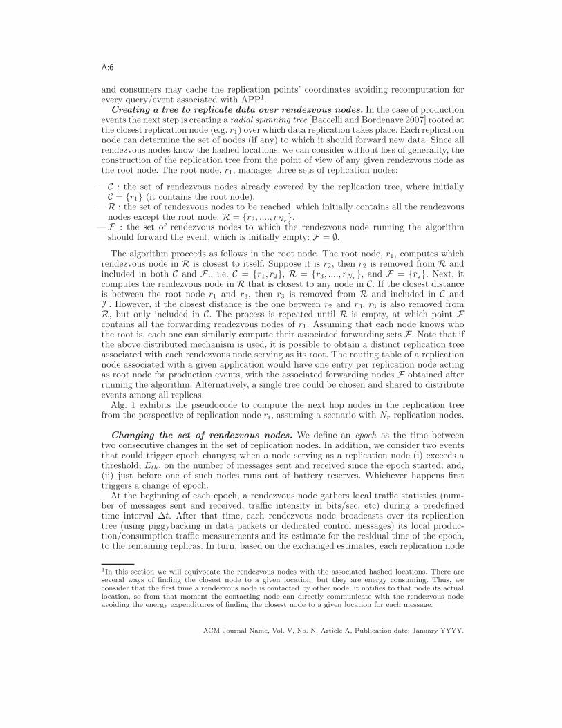
Fig. 3. Consumption, production and overall tra!c generated by using di"erent number of replication nodes(A=1000x1000 m2, N=5000 nodes, !=200 bits, "=100 bits) for the case when consumption dominatesproduction

grows as "x2!!r!2

, so the average length of the tree per unit area is given by!!r/2 [Baccelli

and Bordenave 2007]. The total production tra!c generated, Tp(!r), is thus given by # bitsper event, times the rate of production events !pA in the network, times the length of theassociated radial spanning tree:

Tp(!r) = #!pA

"!r

2A = #A2!p

"!r

2bits·m/s.

Note that we have assumed for simplicity that the radial spanning tree is rooted at thelocation where the event is produced. Alternatively one could assume that the new event isfirst transported to the nearest replication node that then employs a radial spanning tree toreach the remaining replicas. The replication cost in this second case has a similar scaling.

The total network tra!c, T (!r), is thus given by:

T (!r) = Tc(!r) + Tp(!r) = "A!c1

2(!r

+ #A2!p

"!r

2bits·m/s.

We can optimize this to obtain an optimal spatial intensity for replicas !"r given by:

!"r ="!c(2#A!p

replicas/m2,

and the associated minimum overall network tra!c is given by:

T (!"r) = 21/4(

A#

("!cA)(#!pA) bits·m/s.

Remark 3.1. Scaling characteristics. Roughly speaking the optimal average numberof replicas for the network covering an area A is given by:

N"r = !"rA =

"!c(2#!p

replicas, (1)

This only depends on the ratio of the intensity of consumption to production. Thus if onewere to double the intensity of consumption and production for a fixed area, the samenumber of replicas would be optimal. If however one stretches the area by a factor of two,this would decrease the intensity of production and consumption by 2, maintaining the sameratio, yet the optimal intensity !"r per unit area would also have to decrease by a factor of2. Furthermore we note that the overall network load, in bits·m/s scales as

(A times the


A:12

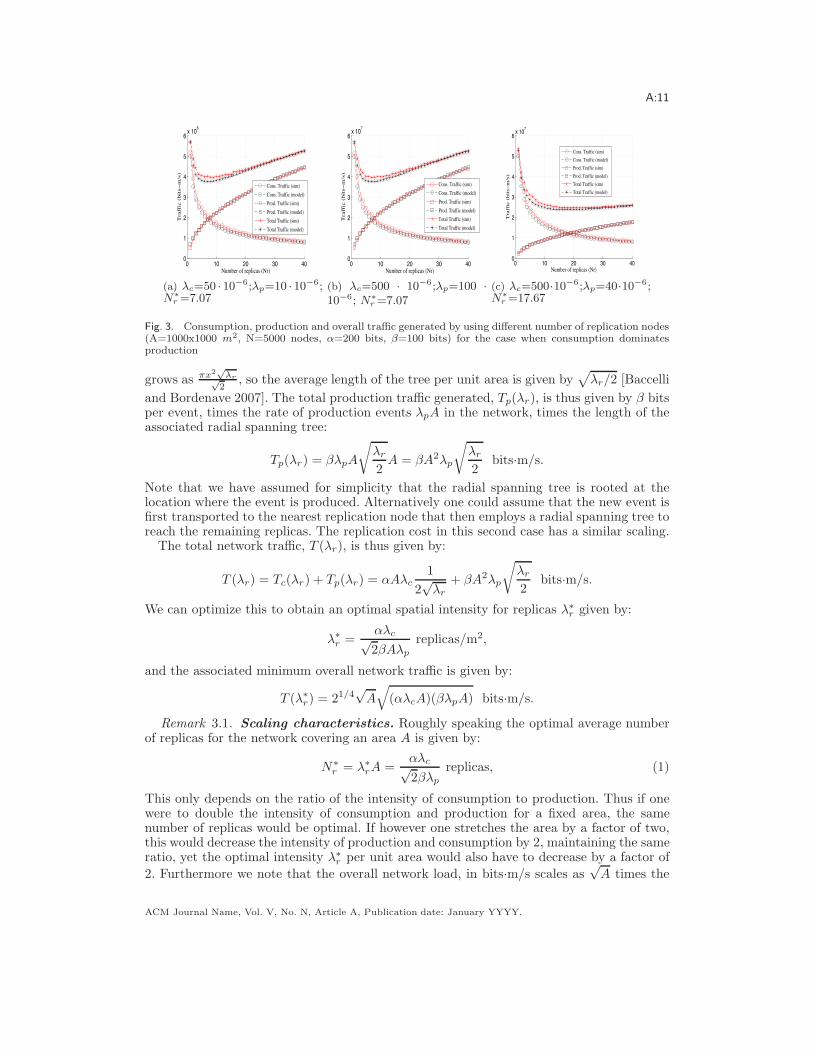
Fig. 4. Optimal number of replicas that minimizes the overall number of messages (A=1000x1000 m2,N=5000 nodes, Tx=50 m)

geometric mean of the total rate of consumption, "!cA in bits/s and the rate of production#!pA in bits/sec. This gives a sense of the growth of overall tra!c with network size.

In order to validate this model we have first simulated random realizations of the net-work and obtained the consumption (Tc), production (Tp) and total network cost (T ) fordi"erent numbers of replicas. Unless otherwise stated, all results correspond to at least 50simulations of di"erent network realizations where N = 5000 nodes are randomly placed ina 1000)1000 m2 region. We set #=100 bits, assuming that producers periodically send theinformation to the closest replica without any acknowledgment. We set "=200 bits since weassume that a consumer first sends a query message to its closest replica and then receivesa reply from it. We show 90% confidence intervals on all graphs unless they are so smallthat they cannot be distinguished.

Figure 3 exhibits the overall consumption, production and total tra!c measured inbits·m/s obtained by the model and by simulation for three di"erent (!c,!p) pairs: (50·10#6,10 · 10#6), (500 · 10#6, 100 · 10#6) and (500 · 10#6, 40 · 10#6) events

s·m2 . The number of replicasemployed varies from 1 to 40. Thus, the optimal average number of replicas for these casesis 7.07, 7.07 and 17.67 respectively. Figures 3(a) and 3(b) illustrate the scaling properties ofthe framework versus the ratio of consumer to producer intensities. Note that both scenar-ios have exactly the same optimal number of replicas, even though the latter’s applicationgenerates ten times more production and consumption events than the former. It is worthnoting that for applications with a high !c/!p ratio (see Figure 3(c)), there are severalvalues around the optimal number of replicas that could be employed instead, because theygenerate a similar overall tra!c.

It must be highlighted that this simple model establishes tra!c metrics assuming routesfollow straight lines. However, WSANs, which are the focus of this paper, are multi-hop


A:13

0 10 20 30 400

0.5

1

1.5

2

2.5

3

3.5

4

4.5 x 107

Tra

ffic

(bi

tsm

/s)


Consumption Traffic (sim)Consumption Traffic (model)Production Traffic (sim)Production Traffic (model)Total Traffic (sim)Total Traffic (model)

(a) !c=10·10!6;!p=200·10!6;N"

r =2.92

0 10 20 30 400

1

2

3

4

5 x 107

Tra

ffic

(bi

tsm

/s)



(b) !c=10·10!6;!p=400·10!6;N"

r =4.64

0 10 20 30 400

1

2

3

4

5 x 107

Tra

ffic

(bi

tsm

/s)



(c) !c=10·10!6;!p=700·10!6;N"

r =6.74

Fig. 5. Consumption, production and overall tra!c generated by using di"erent number of replicationnodes (A=1000x1000 m2, N=5000 nodes, !=200 bits, "=100 bits) for the case when production dominatesconsumption.

networks where routes unlikely follow straight paths. To that end we have verified thatfor networks that have a su!ciently high density of nodes, the optimal number of replicasobtained by our idealized model reflects the actual optimal number of replicas on a givennetwork. For this purpose we have simulated a WSAN employing greedy forwarding [Karpand Kung 2000] and a transmission range Tx = 50 m. We have considered a setup wherethe ratio !c/!p varies from 1 to 25.

Figure 4 shows the number of replicas that minimizes the overall simulated tra!c basedon the actual number of hops of all messages compared to the optimal number of replicassuggested by our model. As can be seen, when there is a low number of replicas, the modeland the simulations are a good match. A small discrepancy occurs for high !c/!p ratios.However, as mentioned earlier, in the case this ratio is high, the overall cost is not verysensitive to the precise optimal value for the number of replicas.

Case 2: Production dominates consumption (!c < !p). If the intensity of consumption is lowrelative to that of production it may be preferable not to copy data across all replicationpoints. Instead producers can store data solely at the closest replication node. Subsequentlyconsumers should contact all replication points to gather information on their queries. Thiscould be done in several ways2 although we will consider the simplest one where consumerscontact all the replication points directly.

In this case the overall production tra!c is:

Tp(!r) = #A!p

2(!r

bits·m/s.

The consumption cost can be modeled using the average distance between any two nodesof the network

(A/2, as the distance from a consumer to each replica, times the number

of consumers and replicas. Thus the overall consumption tra!c is given by:

Tc(!r) = "(!cA)(!rA)(

A

2bits·m/s.

2A symmetric model to that presented in the case of consumption dominating production could be alsoproposed. However, that model would assume that both, queries and replies, are sent through the replica-tion tree once per branch. This can only be achieved if replies are aggregated, but such aggregation hasimplications that are out of the scope of this paper.


A:14

The total network tra!c is then given by:

T (!r) = "!c!rA2

(A

2+ #A

!p

2(!r

bits·m/s.

One can again find the optimal replication !"r for this case, which is given by:

!"r =1A

$#!p

2"!c

%2/3

replicas/m2.

The associated minimum overall network cost is:

T (!"r) = (#!p)2/3 (2"!c)

1/3 3A(

A

4bits·m/s.

Note that in this regime the optimal intensity of replicas is a more ‘complex’ function,i.e., cubic of the ratio of production to consumption intensities, yet, in principle, still easilycomputable by nodes in the field. This model has been also validated via simulation. Figure 5shows the overall consumption, production and total tra!c measured in bits·m/s comparedthe model and the simulation results for three di"erent (!c,!p) pairs: (10 · 10#6,200 · 10#6),(10 · 10#6,400 · 10#6) and (10 · 10#6,700 · 10#6) events

s·m2 . The number of replicas employedvaries from 1 to 40. Thus, the optimal number of replicas for these cases is 2.92, 4.64 and6.74 respectively. As seen in the figure the model is very close to the simulation results.

3.2. Evaluating storage limits

If multiple applications share the same network storage resources, say a storage capacity ofb bits per node, this may limit the amount of replication one can use. To better understandthis, consider a network where m homogeneous applications, i.e., with the same consumptionand production intensity and data storage requirements, say d, share a network with anintensity of !n nodes/unit area in region A.

To model memory utilization in replication nodes, suppose a given application selects thenodes to serve as replication nodes as follows. It generates random spatial locations $r withintensity !r on the plane, and then network nodes that are the closest ones to these locationsare chosen as replication nodes. Note if several points in $r are close to the same node, thenthat node is used only once. Let V be a random variable denoting the area of the Voronoicell of a typical network node. If at least one point in $r is in the Voronoi cell of such node,it is selected as a replica. The probability that the region with area V = V contains nopoint from the process a $r locations, is given by its void probability p(V) = e#!rV [Stoyanet al. 1995]. So the average probability a typical node is chosen by an application using aintensity !r for choosing replication nodes is given by:

1 * E[p(V )] = 1 * E[e#!rV ] + !rE[V ] * !2r

2E[V 2] =

!r

!n* 0.62

!2r

!2n

where we have used the fact that E[V ] = 1!n

and also that!

Var(V ) = E[V ](0.52) [Moller1994].

Let Xi be a Bernoulli random variable which is 1 if application i uses the node as areplication site, and zero otherwise, i.e.,

P (Xi = 1) = 1 * E[p(V )] and P (Xi = 0) = E[p(V )].Suppose a given node has enough storage for b/d di"erent application’s data, then theprobability that it is overloaded is given by:

P (m&

i=1

Xi > b/d).


A:15

8 10 12 14 16 18 206

8

10

12

14

16

18

20

Number of applications (m)

Max

. rep

licas

per

app

licat

ion

Storage modelSimulation

Fig. 6. Maximum number of replicas per application to keep the probability of node saturation below a10% (A=1000x1000, N=100, b/d=3, #=0.1).

Note that Xi are not independent, because if a cell has a larger area, they are more likely tobe 1. In other words they are only conditionally independent given the area of the cell. Toestimate the overload probability, we shall still approximate the above sum as a Gaussianrandom variable, i.e.,

'mi=1 Xi , N(µ,$2) where µ and $2 correspond to the mean and

variance of the sum. In particular, as shown above:

µ = E[m&

i=1

Xi] + m!r

!n* 0.62

!2r

!2n.

To compute the variance of the sum we can condition on the size of the cell V to obtain:

$2 = Var(m&

i=1

Xi) = E[Var(m&

i=1

Xi|V )] + Var(E[m&

i=1

Xi|V ])

= E[mp(V )(1 * p(V )] + Var(m(1 * p(V )))= mE[p(V )(1 * p(V )] + m2(E[(1 * p(V ))2] * E[1 * p(V )]2).

Further expanding the terms in the previous equation, we obtain:

$2 + m

$!r

!n* 1.9

!2r

!2n

%+ m2

$0.27

!2r

!2n

+ 1.27!3

r

!3n

* 1.61!4

r

!4n

%.

Now given these results we can roughly assure that the risk of running out of storagespace for a typical sensor is less than % by requiring that:

P (m&

i=1

Xi >b

d) + Q(

bd * µ

$) - %


A:16

where Q() denotes the complementary distribution function of a standard Gaussian randomvariable. This in turn gives a requirement that

b

d. µ + t(%)$

where t(%) is such that Q(t(%)) = %.This can be interpreted as a constraint on the maximum number of homogeneous appli-

cations one can support, or the maximum replication rate per application one can allow.In order to validate the model, we simulated a network where the requirements on nodes’

storage were fairly high. This is the case where the Gaussian approximation is e"ective andthe model can provide useful results for network designers. Specifically we have simulated anetwork with N = 100 nodes, and varied the number of applications from 8 to 20, and thenumber of replicas per application from 1 to 20. We considered the case where b/d = 3, i.e.,a node can simultaneously support at most 3 applications. For each scenario we evaluatedthe maximum number of replicas each application could use while ensuring that a typicalnode’s saturation probability was lower than % = 0.1 both via simulation and with ouranalytical model. Figure 6 shows that the storage model and the simulation results are veryclose, showing a di"erence of just 1 replica in most of the cases. Moreover, it must be notedthat the model is conservative, since it provides a lower value than the simulation, which isdesirable for safe network design.

The importance of these results is as follows. When multiple applications share the net-work infrastructure, our analysis shows that depending on the production and consumptionintensity they may choose to use a large number of replicas. However in doing so, it mayrequire replicas to store more data than they are in fact capable of. So in practice theintensity of replication associated with multiple information services sharing the networkmay need to be limited, to preclude this overload from happening.

3.3. Cost of changing the set of replication nodes to balance network loads.

We have argued that it would be worthwhile to periodically change the set of nodes wheredata is replicated. The cost of moving from one set of replica nodes to another should berelatively low since this is a highly-parallel distributed process. In particular, suppose thecurrent intensity of replicas is !c

r and we wish to move to a new set of randomly-locatedreplicas with intensity !n

r . Note that the new set of replicas does not need to have the sameintensity as the current one. Also suppose each replica node currently holds an averageamount of data s.

A rough estimate of the energy cost associated with moving data from the current set ofreplication nodes to the new one Tr(!c

r ,!nr ), can be evaluated as follows. Each old replica

would contact one of the new nodes. Given that the distance to a new randomly locatedreplica from one of the current nodes is 1

2(

!nr

the total cost in a network of area A would

be roughly:

Tr(!cr ,!

nr ) =

s

2!c

rA!!n

r

. bits·m

So if !nr = !c

r the cost is Tr = s2

(!r bits-m. If the set of replication nodes changes in-

frequently, then the contribution to the overall network tra!c and energy consumption ofchanging the set of replicas would be fairly small. However this does depend on !r and thefrequency of such updates. We shall consider this in more detail in the next section.

4. PERFORMANCE EVALUATION

In this section we consider two questions: (1) how selecting rendezvous nodes’ locations atrandom compares to previous grid-based and uniform-based proposals; and (2), whether it


A:17

0 10 20 30 400

10

20

30

40

50

60

Consumption to Production ratio ( c/ p )

Ove

rhea

d tr

affi

c co

mpa

red

to R

ando

m R

epli

cati

on (

%)

ToWGHTGHT multireplicaScaling LawsQAR

(a) Overhead tra!c of other solutions when com-pared to Random

0 10 20 30 400

10

20

30

40

50

60

70

Consumption to Production ratio ( c/ p)

Opt

imal

Num

ber

of R

epli

cas

(Nr*

)

ToWScaling LawsQARRandom Replication

(b) Number of replicas used for the di"erent propos-als: ToW, QAR, Scaling-Laws and Random

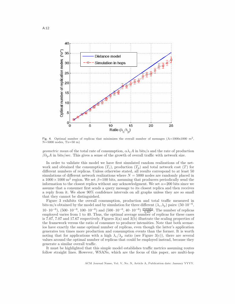
Fig. 7. Random vs. ToW, QAR, Scaling-Laws, GHT and GHT with multiple replicas (A=1000x1000 m2,N=5000 nodes, Tx=50 m, !=200 bits, "=100 bits)

.

is worthwhile to change the set of rendezvous nodes over time considering the associatedoverheads. We have developed a custom simulator that provides more scalability than stan-dard ones, since it does not simulate wireless communications (i.e. PHY and MAC) otherthan transmission range.

4.1. Random vs. grid-based and uniform replica allocation

4.1.1. Quantitative Comparison. We have compared random replication that is the replica-tion mechanism used in the proposed STARR-DCS framework with those that are similarin spirit: ToW [Joung and Huang 2008], QAR [Cuevas et al. 2010], Scaling Laws [Ahn andKrishnamachari 2006], the original GHT proposal [Shenker et al. 2003], which uses a singlereplication node, and GHT with multiple replication nodes [Ratnasamy et al. 2002; Rat-nasamy et al. 2003]. For the last case, since the authors do not propose any way to obtainthe number of replicas to be used, we select the same number used in ToW since both worksare grid-based and use the same 4d geometric formula for the number of rendezvous nodes.

In order to compare these approaches, we ran simulations for a large WSAN with thefollowing characteristics: an area A = 1000 ) 1000 m2, N = 5000 nodes, transmissionrange Tx = 50 m and !c/!p tra!c ratio ranging from 1 to 40. For each !c/!p ratio we havesimulated 50 scenarios to estimate the mean network cost realized by the di"erent replicationapproaches. In order to get meaningful results, we use the number of hops traversed by allmessages as the measure of the overall tra!c cost.

Figure 7(a) shows the network tra!c improvement achieved using random replicationcompared to all the other approaches, and Figure 7(b) depicts the number of replicas usedby each approach for each particular !c/!p ratio.

Random replication reduced the overall tra!c by an average of 137% compared to GHT,39% compared to Scaling Laws, 21% compared to GHT with multiple replication nodes,4% compared to ToW and 1.5% compared to our previous QAR proposal. Moreover, thisimprovement reaches peaks around a 50% when compared to Scaling Laws and GHT withmultiple replicas, 15% to ToW and 7% to QAR.

The main reason our solution achieves a better performance, is that it allows a finergranularity at which the number of replicas being used can be fine tuned. That is, the


A:18

optimal number of replicas grows linearly, whereas ToW and GHT with multiple replicasemploy a 4d geometric growth and QAR a quadratic one (see Figure 7(b)). For instance, insome cases ToW must choose between 16 or 64 replicas, where none of them is a good fitfor the scenario of interest.

We conclude that random replication is the approach best minimizing the overall networktra!c improving over all previous approaches in the literature that use grid-structured oruniform replication. Moreover, processing the random locations for the rendezvous nodes iseasier for di"erent sensornet shapes than those using structured replication. Hence, randomreplication is simpler and more cost-e"ective. Therefore, all these results validate our op-tion of choosing random replication as the replication mechanism in the proposed solutionSTARR-DCS.

4.1.2. Qualitative Comparison. It must be noted that the use of randomly-located replicationnodes can be used whatever the underlying routing protocol is as long as it is able toidentify routing addresses for replication nodes. However, structured replication mechanismssuch us ToW [Joung and Huang 2008], QAR [Cuevas et al. 2010], Scaling-Laws [Ahn andKrishnamachari 2006] and GHT with multiple replicas [Ratnasamy et al. 2002], can beonly applied when geographic routing is used. Therefore, if we think of a distance vectoror link-sate routing protocol based on node-ID in which a node knows at least the nexthop towards a given destination, it is simple to select a random set of replication nodes.However, by just knowing the nodes ID, it is not possible to allocate the replication nodes ina grid fashion because the nodes do not know their own location information, and thereforethe set of nodes creating a grid replication structure cannot be found.

Therefore, the only approach that works with an important number of ad-hoc routingprotocols (e.g. pathDCS [Ee et al. 2006]) is random replication.

4.2. Changing Replicas over the time

Nodes selected as rendezvous nodes (and those close to them) will naturally expend moreenergy than other nodes. Thus, if the responsibilities of nodes do not change, those nodesare most likely to run out of energy reserves first. In [Shenker et al. 2003], [Ratnasamy et al.2002], [Ratnasamy et al. 2003], [Cuevas et al. 2010] and [Joung and Huang 2008], when thishappens, an alternate node close to the previous replication point is selected as the newrendezvous node, until its battery expires, and so on. After some time, routing (and sensing)holes will be created around the original replication coordinates, a"ecting the routing of thewhole network.

If replication points change over time, the extra energy expenditures associated withrendezvous nodes can be balanced across all the nodes in the network, thus extendingthe network’s lifetime, and avoiding the creation of routing holes. In addition, althoughmoving replication points has an associated overhead, this does not mean that networkenergy expenditures become higher than keeping rendezvous nodes static. Indeed, whenreplication nodes are kept static, longer paths will be required to avoid routing holes, whichin turn will consume more energy. In this section we demonstrate that routing holes canhave more impact on the overall network energy expenditures than the cost of changing theset of rendezvous nodes over time.

In order to verify the abovementioned statements, we ran simulations comparing ToW[Joung and Huang 2008] that uses static replicas (ToW-static) with STARR-DCS, wherethe set of replication nodes changes over the time.

We use a grid-based node deployment (which makes energy maps generation easier) withN = 900 nodes, over a square of area A = 300)300 m2. Each node has a transmission rangeTx = 30 m. In addition, it must be noted that we evaluate the case where consumptiondominates production (!c > !p). We use the number of messages in the network as a firstorder proxy for consumed energy. A sensor node’s energy is depleted once it sends and/or


A:19

(a) ToW-Static after30K cycles

(b) STARR-DCS after30K cycles

(c) ToW-Static after50K cycles

(d) STARR-DCS after50K cycles

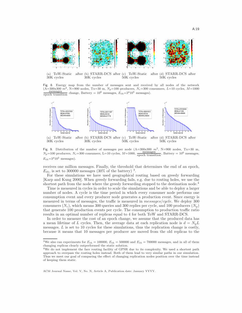
Fig. 8. Energy map from the number of messages sent and received by all nodes of the network(A=300x300 m2, N=900 nodes, Tx=30 m, Np=100 producers, Nc=300 consumers, L=10 cycles, M=1000

messagesepoch transition change, Battery = 106 messages, Eth=3*105 messages).

0 100 200 300 400 500 600 700 800 9000

2

4

6

8

10

12x 105

Sorted node list

Nu

mb

er

of

Me

ssa

ge

s

TOTAL=223157503MEAN=247950MEDIAN=90000

(a) ToW-Static after30K cycles

0 100 200 300 400 500 600 700 800 9000

2

4

6

8

10

12x 105

Sorted node list

Nu

mb

er

of

Me

ssa

ge

s


(b) STARR-DCS after30K cycles

0 100 200 300 400 500 600 700 800 9000

2

4

6

8

10

12x 105

Sorted node list

Nu

mb

er

of

Me

ssa

ge

s


(c) ToW-Static after50K cycles

0 100 200 300 400 500 600 700 800 9000

2

4

6

8

10

12x 105

Sorted node list

Nu

mb

er

of

Me

ssa

ge

s TOTAL=370164530MEAN=411290MEDIAN=389906

(d) STARR-DCS after50K cycles

Fig. 9. Distribution of the number of messages per node (A=300x300 m2, N=900 nodes, Tx=30 m,Np=100 producers, Nc=300 consumers, L=10 cycles, M=1000, messages

epoch transition , Battery = 106 messages,

Eth=3*105 messages).

receives one million messages. Finally, the threshold that determines the end of an epoch,Eth, is set to 300000 messages (30% of the battery) 3.

For these simulations we have used geographical routing based on greedy forwarding[Karp and Kung 2000]. When greedy forwarding fails, e.g. due to routing holes, we use theshortest path from the node where the greedy forwarding stopped to the destination node.4

Time is measured in cycles in order to scale the simulations and be able to deploy a largernumber of nodes. A cycle is the time period in which every consumer node performs oneconsumption event and every producer node generates a production event. Since energy ismeasured in terms of messages, the tra!c is measured in messages/cycle. We deploy 300consumers (Nc), which means 300 queries and 300 replies per cycle, and 100 producers (Np)that generate 100 production events per cycle. The consumption to production tra!c ratioresults in an optimal number of replicas equal to 4 for both ToW and STARR-DCS.

In order to measure the cost of an epoch change, we assume that the produced data hasa mean lifetime of L cycles. Then, the average data at each replication node is d = NpLmessages. L is set to 10 cycles for these simulations, thus the replication change is costly,because it means that 10 messages per producer are moved from the old replicas to the

3We also ran experiments for Eth = 100000, Eth = 500000 and Eth = 700000 messages, and in all of themchanging replicas clearly outperformed the static solution.4We do not implement the face routing facility of GPSR due to its complexity. We used a shortest pathapproach to overpass the routing holes instead. Both of them lead to very similar paths in our simulation.Thus we meet our goal of comparing the e"ect of changing replication nodes position over the time insteadof keeping them static.


A:20

Table I. WSAN Lifetime ToW-Static vs STARR-DCS

Lifetime 1st 1% 10% 25% 40% 10% 25% NetworkCriteria dead dead dead dead dead cons+prod cons+prod disconnectionToW-Static (cycles) 2619 7328 29086 47830 63230 31668 47984 70952STARR-DCS (cycles) 31199 41124 66750 87968 101523 65171 79717 170950Improvement(%) 1091% 461.2% 129.5% 83.9% 60.6% 105.8% 66.13% 140.9%

new ones. By having 100 producers, this means a total cost of M=1000 messages per epochchange.

Figure 8 shows the energy distribution map after a simulation time of 30000 and 50000cycles. Figure 9 shows the number of messages sent and received by each node at the samecycles, as well as the mean and median values per node and the total messages sent andreceived in the whole network, that roughly captures the total energy consumed by thenetwork.

As seen in Figures 8(a) and 8(c), keeping static replication points creates routing holesin the network, with 93 and 247 expired nodes after 30000 and 50000 cycles respectively.The number of depleted nodes are only 0 and 17, respectively, when replication nodes arechanged over the time, that is, when STARR-DCS is in place. Furthermore, simulationresults obtained later in time (70959 cycles) show that ToW-static network is eventuallydisconnected, because holes become very large and coalesce. In addition, more nodes par-ticipate in the network operation when STARR-DCS is used. As shown in Figure 9, allnodes except 18 (2%) after 30000 cycles and 15 (1.7%) after 50000 cycles, have sent and/orreceived at least one message, whereas in the case of ToW-static more than 200 (22%) nodeshave not sent or received any message after 30000 cycles, decreasing to 160 (17.8%) nodesafter 50000 cycles. When considering the total energy consumed by the network, STARR-DCS uses just 0.8% more energy than the static one after 30000 cycles. However, a 3.3%extra energy is required by the static approach after 50000 cycles. This shows that the costof using longer routing paths eventually exceeds that of changing the rendezvous nodes overtime.

In Table I, we compare the network lifetime using both approaches: ToW-static andSTARR-DCS. Since lifetime can be defined using di"erent metrics [Dietrich and Dressler2009] (first node running out of battery, some percentage of nodes running out of battery,important nodes like consumers and/or producers running out of battery, some part ofthe network disconnects and many messages are lost, etc), we provide a broad overviewof metrics to let the reader establish a fair comparison depending on the criterion used todefine the network’s lifetime. The table shows the number of cycles spent until each lifetimecriterion is reached. For all the criteria our solution extends the network’s lifetime by atleast 60%. We note that in many cases changing replicas over the time and using randomreplication extends the network’s lifetime by a factor of 2x.

Finally, Figure 10 shows how using a message threshold to trigger epoch changes com-pares to employing a fixed epoch duration as proposed in [Thang et al. 2006] (note thatthis work actually refers to a single rendezvous node scenario and it proposes to changemotivated by storage saturation instead of energy issues). We simulate a larger (N=5000nodes, A=1000 ) 1000 m2, Tx=50 m) multi-application WSAN with random replication.We set up m=5 heterogeneous applications with (20, 40), (60, 120), (100, 200), (140, 280)and (180, 360), (production-events

cycle , consumption-queriescycle ) pairs, calculating the network’s

lifetime (1% of nodes expire) for both the two dynamic approaches versus using a fixedstatic set of randomly located replicas. Again the need for changing replicas over the timeversus using static ones is clear. In addition, as seen in the figure, our proposal to triggerepoch changes based on message counts is more robust to the precise setting of the messagethreshold than using a fixed epoch duration. That is, the set of values providing good values


A:21

Fig. 10. WSAN lifetime comparison (A=1000x1000 m2, N=5000 nodes, Tx=50 m, L=10 cycles, m=5applications, Battery=106 messages). X axis refers to the cycles for changing the epoch in the fixed durationapproach, or the message threshold.

of network lifetime represents a very small window when employing fixed epoch durationwhereas our solution shows a larger window to choose a message threshold value leading toa good network lifetime.

4.3. Epoch duration analysis

We have already demonstrated the great improvement of changing the replication nodesover the time. Thus the next question is whether it is better to use shorter or longer periodsbefore an epoch transition. At first glance, the best solution seems to be using short periodsso that the load is better spread among the nodes. However, as we have already seen, thereare some overheads associated with epoch transitions, such as moving all the data storedin the current replicas to new ones. Considering this trade-o", using shorter epoch periodswill lead to balance the energy consumption among the nodes, thus reducing the energyconsumption variance per node, but it would also increase the average energy expendituresper node, which means increasing the overall energy expenditure. By contrast, using longerepoch periods increases the variance of thexww node energy consumption since nodes willkeep being replicas for more time, but it will reduce the overall (average) tra!c on thenetwork.

Thus the key of this trade-o" is determining how much extra energy should be spent tobalance the energy among the nodes. The decision depends on each particular application.For instance, for an application where all the nodes are needed, so that all of them shouldkept alive together in order to allow the application to work properly, (i.e. extend the timewhen the first node runs out of battery) the right selection is to balance the energy as muchas possible, by means of using short epochs (frequent epoch changes). Of course the price ofdoing so is that a lot of extra energy is required for those frequent epoch changes. Thus, if


A:22

1 1.5 2 2.5 3 3.5 4 4.5 50

15

30

45

60

75

% re

lativ

e en

ergy

exp

endi

ture

s

Cycles per epoch (log scale)

1 1.5 2 2.5 3 3.5 4 4.5 50

0.2

0.4

0.6

0.8

1

Fairn

ess I

ndex

(FI)

Extra Energy

Fairness Index

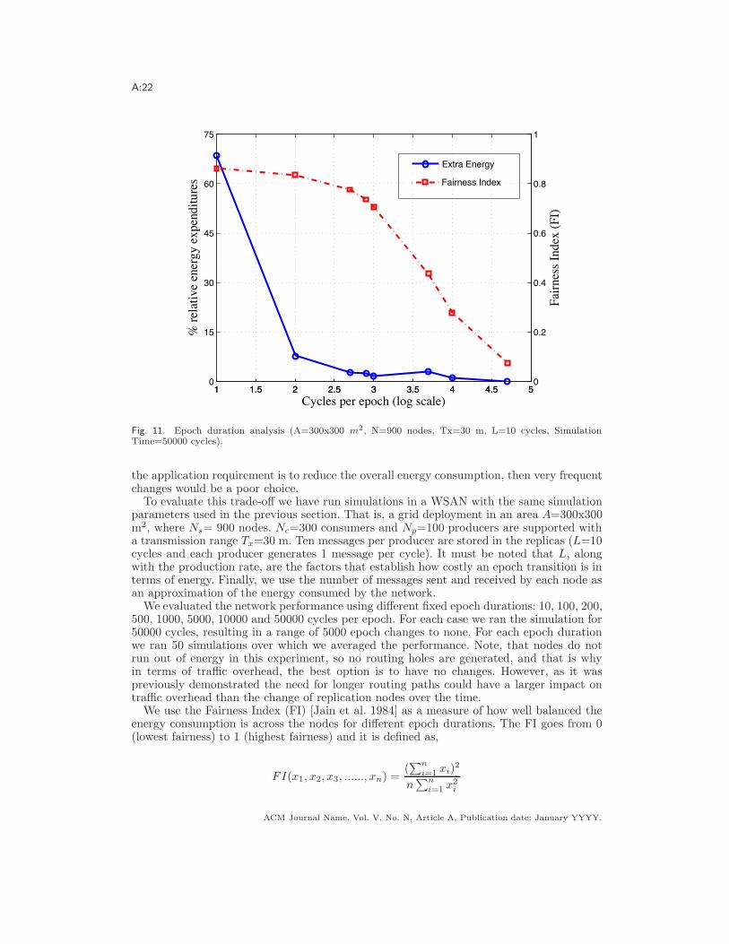
Fig. 11. Epoch duration analysis (A=300x300 m2, N=900 nodes, Tx=30 m, L=10 cycles, SimulationTime=50000 cycles).

the application requirement is to reduce the overall energy consumption, then very frequentchanges would be a poor choice.

To evaluate this trade-o" we have run simulations in a WSAN with the same simulationparameters used in the previous section. That is, a grid deployment in an area A=300x300m2, where Ns= 900 nodes. Nc=300 consumers and Np=100 producers are supported witha transmission range Tx=30 m. Ten messages per producer are stored in the replicas (L=10cycles and each producer generates 1 message per cycle). It must be noted that L, alongwith the production rate, are the factors that establish how costly an epoch transition is interms of energy. Finally, we use the number of messages sent and received by each node asan approximation of the energy consumed by the network.

We evaluated the network performance using di"erent fixed epoch durations: 10, 100, 200,500, 1000, 5000, 10000 and 50000 cycles per epoch. For each case we ran the simulation for50000 cycles, resulting in a range of 5000 epoch changes to none. For each epoch durationwe ran 50 simulations over which we averaged the performance. Note, that nodes do notrun out of energy in this experiment, so no routing holes are generated, and that is whyin terms of tra!c overhead, the best option is to have no changes. However, as it waspreviously demonstrated the need for longer routing paths could have a larger impact ontra!c overhead than the change of replication nodes over the time.

We use the Fairness Index (FI) [Jain et al. 1984] as a measure of how well balanced theenergy consumption is across the nodes for di"erent epoch durations. The FI goes from 0(lowest fairness) to 1 (highest fairness) and it is defined as,

FI(x1, x2, x3, ......, xn) =('n

i=1 xi)2

n'n

i=1 x2i


A:23

where xi represents the number of messages sent and received by node i. In addition, wemeasure the relative energy expended in the network for di"erent epoch durations (moreor less changes during the simulation time) compared to the minimum energy case (i.e.no changes). Figure 11 shows the FI and the relative energy consumed for di"erent epochdurations on a logarithmic scale.

As we could expect, the lower the number of epochs per cycle (the more epoch changes)the better the network fairness, but the greater the overall energy required. However, thereis a region, around 500 cycles per epoch (between 2.5 and 3 in the x-axis in the figure), wherethe extra energy consumed is not that big, below a 5%, and the FI is very good (>0.75).This operational regime heavily depends on the value of L, which impacts the overheadassociated with epoch changes. If this cost is low this region moves to the left, resulting ina better FI and a lower energy requirement. However, if the transition cost is very high,the region with a low energy demand (compared to the best case) will move to the right, ofcourse producing worse FI values, thus a bigger variance for the energy consumed per node.Although the abovementioned region could be a good operational regime area in general,we note that each application may have a di"erent suitable operational regime.

5. STARR-DCS IMPLEMENTATION

We have implemented STARR-DCS on real motes. Our implementation supports an arbi-trary number of replicas that change over the time, and uses the Meta-Information servicefor bootstrapping purposes. Furthermore, replicas are able to exchange tra!c measurementsand compute the remaining time of the current epoch, as well as the number of replicas forthe next epoch. These provide an e!cient synchronization mechanism for all the entitiesinvolved in a particular application: consumers, producers and replication nodes.

To test the implementation we have used 20 Jennic motes of two di"erent types: JN-5121(5x) and JN-5139 (15x) . The JN-5139 wireless microcontroller device integrates a 32-bitRISC processor, with a fully compliant 2.4GHz IEEE 802.15.4 transceiver, 192kB of ROM,96kB of RAM, and several analogue and digital peripherals. The JN-5121 is an older versionand it only has 64kB of ROM.

5.1. Implementation details

A node can initially be assigned one of these three roles: producer, consumer or relay (inwhich case it is neither a consumer nor a producer). The role of a particular node is expectedto be specified by the application using the framework.

Producers generate events via two di"erent mechanisms: (i) at a predefined rate, e.g.temperature reading every minute; (ii) manually when a button is pressed. Moreover, thenumber of data elements per event can be configured by the application (e.g. three tem-perature samples per production event). Consumers also generate queries using the samemechanisms utilized by the producers: at a constant query rate or triggered by a pressedbutton.

We implemented a greedy forwarding routing on the motes as the routing layer to be usedby our framework. In order to avoid more complex routing operations (e.g. face routing),we set up scenarios in which it was feasible to route a message from any source to anydestination node by only using greedy forwarding. In these scenarios, if a node receives amessage and it is closer to the destination coordinates than any of its neighbours, then itis the closest one to the destination coordinates. The mechanism used to choose the nodesacting as replicas is the closest one to a randomly selected spatial location.

We have defined a common header to be used by all the protocol messages required toimplement the STARR-DCS framework. Figure 12 shows all the di"erent fields included inthe header. Next, we describe each of these fields:


A:24

Fig. 12. Protocol Header to implement STARR-DCS.

— OPERATION CODE: Defines the type of message (e.g., PUT, GET, GET REPLY,etc).

— FLAGS: Is used for special operations, i.e. consumers and producers use a flag to indicatethat they do not know yet when the current epoch finishes and what is the number ofreplicas to be used in the next epoch. This field is also used to request an acknowledgement.

— APPLICATION ID: Defines the application that is using the framework.— DATA TYPE: Is used to define the data structure employed by the application,— LENGTH: Indicates how many data structures are included in the message.— REPLICA INDEX: Identifies (in the case that is required) the replication node that is

the source of the message (e.g., that information is needed in all the replication nodes inorder to generate the replication tree in a distributed fashion).

— EPOCH ID: Specifies what is the current epoch of the source node and it is used forsynchronization purposes.

Next, we present all the di"erent message types required in our implementation that areidentified by di"erent OPERATION CODE values:

— PUT: Is the message used by producers to send the measured data to the closest repli-cation node. In addition, it is also used for updating the epoch and number of replicas ofa given application stored in the Meta-Information service. Then, once the replicas haveobtained the epoch expiration time and the number of replicas in the next epoch, thefirst one (assigned the ID 1 in the hash operation) sends a PUT message to the Meta-Information service node, indicating the next epoch ID, the number of replicas in the nextepoch and the time in seconds until the current epoch expires (similarly as it is done withconsumers and producers). Therefore, the Meta-Information service node sets up a timerthat ends at the end of the current epoch, until that moment it still serves the informationfor the current epoch, after it will start serving the information of the next epoch. Whenthe PUT message is used to update the Meta-Information service information a flag isused to indicate that an acknowledgement is required.

— PUT ACK: Is the message used to acknowledge a PUT message that requires a confir-mation.

— EPOCH ADVERTISEMENT: This message is used to notify producers about theepoch duration and the number of replicas to be used in the next epoch. Then, thismessage contains the number of replication nodes that will be deployed in the next epochand the time in seconds until the end of the current epoch.

— GET: Is the query message used by consumers to obtain information from the closestreplica. GET messages are also used when a new producer or consumer contacts theMeta-Information service in order to obtain the current epoch and number of replicationnodes of the application it wants to participate.


A:25

Fig. 13. Real testbed using 20 motes emulating a 200x200 square meter network in a two dimensions plane

.

— GET REPLY: Is the message that answers consumers’ (or producers’ when using theMeta-Information service) GET request. It contains the suitable application informationrequested by the consumer (or producer). In addition, the information about the epochduration and the number of replicas to be used in the next epoch is piggybacked in thismessage for consumers. .

— REPLICATION: Is the message used to replicate the production data received by onereplica in the remaining replicas.

— REPLICATION STATISTICS: Is a message used by a replica to send other onesthe consumption and production tra!c accounted during the measurement period. Thismessage is sent through the replication tree and it is retransmitted after a pre-definedtime if some acknowledgement is not received.

— REPLICATION STATISTICS ACK: Each replica receiving a REPLICATIONSTATISTIC message sends an ACK back to the source node in order to notify that itreceived the measurement information. This message does not use the replication tree butit is sent using a direct path.

— REPLICA INSTANTIATION: When the epoch expires, old replicas send a REPLICAINSTANTIATION message to the suitable new replication nodes, which become replicasfor the new epoch after receiving this message.

— REPLICA INSTANTIATION ACK: New replicas acknowledge the ones in the pre-vious epoch that they have been instantiated and they are performing the replica role inthe new epoch.

It must be noted that we have implemented the Meta-Information service in a singlestatic node and we have checked that the bootstrapping and fault tolerance services workfine. Therefore, nodes initialized after the application has run during several epochs are ableto synchronize and normally produce or consume data over the time.

Moreover, our implementation covers a multi-application environment. In particular, wesuccessfully ran 4 di"erent applications in parallel on our testbed.


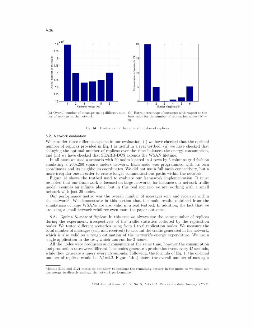
A:26

1 2 3 4 5 61.2

1.25

1.3

1.35

1.4

1.45

1.5

1.55

1.6 x 105


Ove

rall

num

ber

of m

essa

ges

(a) Overall number of messages using di"erent num-ber of replicas in the network.

1 2 3 4 5 60

5

10

15

20


Ext

ra n

umbe

r of

mes

sage

s (%

)

(b) Extra percentage of messages with respect to thebest value for the number of replication nodes (Nr=3).

Fig. 14. Evaluation of the optimal number of replicas

5.2. Network evaluation

We consider three di"erent aspects in our evaluation: (i) we have checked that the optimalnumber of replicas provided in Eq. 1 is useful in a real testbed, (ii) we have checked thatchanging the optimal number of replicas over the time balances the energy consumption,and (iii) we have checked that STARR-DCS extends the WSAN lifetime.

In all cases we used a scenario with 20 nodes located in 4 rows by 5 columns grid fashionemulating a 200x200 square meters network. Each node was programmed with its owncoordinates and its neighbours coordinates. We did not use a full mesh connectivity, but amore irregular one in order to create longer communications paths within the network.

Figure 13 shows the testbed used to evaluate our framework implementation. It mustbe noted that our framework is focused on large networks, for instance our network tra!cmodel assumes an infinite plane, but in this real scenario we are working with a smallnetwork with just 20 nodes.

Our performance metric was the overall number of messages sent and received withinthe network5. We demonstrate in this section that the main results obtained from thesimulations of large WSANs are also valid in a real testbed. In addition, the fact that weare using a small network reinforce even more the paper outcomes.

5.2.1. Optimal Number of Replicas. In this test we always use the same number of replicasduring the experiment, irrespectively of the tra!c statistics collected by the replicationnodes. We tested di"erent scenarios using from 1 to 6 replication nodes. We measure thetotal number of messages (sent and received) to account the tra!c generated in the network,which is also valid as a rough estimation of the network’s energy expenditure. We use asingle application in the test, which was run for 3 hours.

All the nodes were producers and consumers at the same time, however the consumptionand production rates were di"erent. The nodes generate a production event every 45 seconds,while they generate a query every 15 seconds. Following, the formula of Eq. 1, the optimalnumber of replicas would be N"

r =4.2. Figure 14(a) shows the overall number of messages

5Jennic 5139 and 5121 motes do not allow to measure the remaining battery in the mote, so we could notuse energy to directly analyze the network performance


A:27

in the network when forcing the framework to use 1, 2, 3, 4, 5 and 6 replicas. The numberof replicas that minimizes the overall tra!c is 3.

Figure 14(b) shows the extra tra!c generated when using a number of replicas di"erentthan 3. Then if 4 replicas are selected, which is the value chosen by our model, only a 0.5%extra tra!c is generated. The other close value to that obtained from the model is 5 replicas.In this case, the overhead tra!c is an 1%. Finally, if we choose those values far from the oneprovided by our model the extra tra!c grows up to a 5% for 2 and 6 replication nodes andup to a 20% when a single replication node is selected. This demonstrates in a real testbedthat always using a single replication node as proposed in the seminal DCS work [Shenkeret al. 2003] could generate a lot of extra tra!c.

This test demonstrates that even if we are far from the model assumptions (i.e. infinitefield, distance-based model instead of hop-based model, etc) the optimal number of replicasthat the model provides is leading to good results in terms of minimizing the networktra!c (thus to reduce the network energy consumption) eliminating the uncertainty ofwhat number of replication nodes should be used.

5.2.2. Balancing Energy Consumption. The second test we have conducted is to verify whetherchanging the replication nodes over time balances energy consumption per node even thoughit generates extra messages associated to epoch transitions. For that we compare a staticscenario with two dynamic ones implementing STARR-DCS that were configured with dif-ferent message thresholds to change the epoch. We remember that the message thresholdis the maximum number of messages that a node can send and receive while playing therole of replication node. In addition, it must be noted that in this test none node ran out ofbattery since we have a small testbed with only 20 nodes, and thus no network holes appearin the network under the static scenario as it happened in the simulation experiments (seeSection 4). We remember that the appearance of routing holes in the static scenario leads toa larger tra!c overhead than the one related to epoch transitions in the dynamic scenario.However, in the current test the dynamic solution presents a higher overhead due to theabsence of routing holes in the static scenario.

The test ran for 3 hours and all the nodes were consumers and producers at the same time.The production rate was 1 message every 45 seconds and the consumption rate was 1 queryevery 15 seconds. As in the previous example this leads to an optimal number of replicas ofN"

r =4.2, so we decided to use 4 replicas in the static case, whereas the STARR-DCS testsalso started with 4 replicas. After the first epoch, the STARR-DCS framework computedthe number of replicas in the next epoch based on the tra!c statistics captured by thereplicas during the measurement period that lasts 1 minute. It must be noted that usuallythe selected number of replicas was 4, but sometimes one node was taking the responsibilityof two hashed locations, therefore the real number of replicas was actually 3. Finally, wehave used two di"erent values for the message threshold in order to manage shorter andlonger epochs. Those values were 240 and 360 messages respectively. We remember thatshorter epochs are expected to provide a better fairness at the price of a higher overheadsince more messages are generated due to more frequent epoch transitions.

Hence, in order to compute the network fairness we use the Fairness Index (FI) [Jain et al.1984] over the number of messages sent and received by each node. In addition, we alsoaccount the extra number of messages generated by the dynamic scenarios in comparisonwith the static case.

Table II shows the expected results. On one hand, changing the replication set over thetime leads to a much fairer energy distribution in the network than using static replicas.In addition, as we expect the shorter the epoch (a lower message threshold) the betterthe energy distribution. That is the reason why the scenario with a 240 message thresholdpresents a better FI than the one with a message threshold of 360. On the other hand,changing the replication nodes over the time leads to increase tra!c overheads, that in our


A:28

Table II. Evaluation of energy distribution. Fairness Index (FI) of messages sentand received by network nodes and overhead generated by STARR-DCS comparedto a static solution using random replication

Static STARR-DCS 240 STARR-DCS 360FI 0.59 0.83 0.81

Overhead (%) 0.00 10.53 7.04

test was a 10% for the STARR-DCS test with shorter epoch (240 messages threshold) anda 7% in case of using a longer epoch (360 messages threshold).

Moreover, we note that we have used a low message threshold to generate quite a fewepoch changes so as to better see the distribution of the energy consumption within thenetwork. Then, using a 240 message threshold in a 3 hours testbed means 30 epochs (i.e.9-10 changes per hour), while a 360 message threshold leads to 20 epochs (i.e. 6-7 epochsper hour).

Therefore we have confirmed in our testbed that changing the set of replication nodesover the time leads to a much fairer energy consumption distribution within the network.

5.2.3. First node dead lifetime. Due to the reduced number of nodes we were using and thefact that Jennic 5139 and 5121 motes do not allow to monitor the remaining battery in anode, we decided to emulate the node battery lifetime with a limit to the maximum numberof messages sent and received by the nodes.

For that purpose we evaluated: a static scenario with random replicas, and two scenar-ios implementing STARR-DCS with message threshold values of 240 and 360 messages,respectively. For each of these scenarios we measured the time when the first node reaches5000, 6000, 7000, 8000, 9000 and 10000 messages in order to demonstrate that changing thereplication set over the time allows an e"ective lifetime extension.

Table III. Evaluation of lifetime extension when adopting the STARR-DCS solution instead of the staticone. We obtain the time when the first node reaches di!erent thresholds

STARR-DCS STARR-DCS STARR-DCS STARR-DCSLifetime Static 240 360 240 360(# msg.) (sec) (sec) (sec) improv. (%) improv. (%)

5000 3054 4199 3506 37% 15%6000 3659 5142 4556 41% 25%7000 4242 6268 5456 48% 29%8000 4830 7203 6301 49% 30%9000 5419 8362 7187 54% 33%10000 6003 8945 7863 49% 31%

Table III shows the e"ective time extension in percentage of the STARR-DCS solutioncompared to a static one. The first conclusion is that changing the replication set over thetime reduces the charge of the most saturated node in the network. This is translated intoa longer period to reach a given number of messages, which implies a longer time beforerunning out of battery. In particular, when analyzing the scenario implementing STARR-DCS with an epoch message threshold of 240, we check that in all the cases the timeextension is over a 35%, and even overpasses a 50% when the messages limit is established in9000 messages. The time extension for an epoch message threshold of 360 is reduced to valuesbetween a 15% and a 33% depending on the di"erent messages limits. This is happeningbecause a lower message threshold implies a shorter epoch, thus a better distribution ofenergy per node. This reduces the number of messages in the node with more messages atthe price of increasing the overhead in the overall network.

Finally, we note that the trend in the results is that the higher the limit of messages,the longer the time di"erence between the static and the framework solutions. That meansthat if we were able to run very long tests (e.g. 1000 epochs) like the ones evaluated in the


A:29

simulations (see Section 4) the lifetime extension would be much higher, as suggested byTable I for the simulation results.

6. STARR-DCS ADAPTATION FOR SPATIALLY INHOMOGENEOUS TRAFFIC

We have presented a framework for scenarios where consumption and production are roughlyhomogeneously distributed within the network. In addition, not only STARR-DCS, but allprevious works proposing multi-replication DCS systems also assume that consumption andproduction intensities are spatially homogeneous. However, this premise cannot be acceptedin many scenarios in which consumption/production queries/events are more concentratedin some parts of the network than others. Therefore, in this section we consider a di"erentscenario where production and/or consumption intensities are spatially inhomogeneous.

STARR-DCS could easily be extended to this new scenario by using the measurementperiod in which all replicas exchange local tra!c information. This information is used tospawn new replicas in those areas with more tra!c and prune those replication nodes thatare located in areas where there is little tra!c.

In particular, in this section we consider the case in which consumption dominates pro-duction (discussion would be similar for the opposite case). In this case the production tra!cis global since each production event is received by all the replication nodes. However, con-sumption tra!c remains local between a consumer and its closest replica. Therefore, weshould consider the localization of the consumption tra!c to decide which areas of the net-work need more replicas, and which existing replicas could be pruned. When the replicationnodes exchange tra!c statistics they know what is the consumption tra!c of the di"erentreplication nodes. Therefore, each node can compute how many replicas should be assignedto the region supported by the current replica depending on its measured consumptiontra!c.

For instance, let us assume a scenario with 5 replicas in the current epoch, which haveexchanged their measured consumption and production tra!c during the measurementperiod. Suppose the percentage of consumption tra!c for each of the 5 replicas is: 0, 10,40, 0 and 50 percent respectively. Under this tra!c pattern we propose a new distributionfor the 5 replicas in the current epoch: the first and fourth replicas are pruned since theydo not see any consumption tra!c, the second replica deserves to be converted into 0.5replicas since it is only receiving a 10% of the overall consumption tra!c, so we keep thesecond replica without pruning. The third replica should be allocated a 40% of the total of 5replicas, which is 2 replicas, therefore a new replica will be spawned by generating locationswith the hash function until the output coordinates are closer to the second replica than roany of the other replication nodes. Finally the fifth replica deserves 2.5 out of the 5 replicas,so 2 new replicas are spawned whose location are closer to the fifth replica than to any ofthe initial replication nodes.

It must be noted that in the above example we have decided to round the numbers ofreplicas, which means that if a node is assigned a value . 0.5 replicas we decide to assign 1replica (in case 3.5 we assign 4 replicas), thus if the value is < 0.5 we assign 0 replicas. Inmany cases, the number of replicas after the heterogeneous adaptation could be di"erent tothe initial value (e.g. in the previous example after the adaptation there would be 6 replicasin the scenario instead of 5). A more sophisticated algorithm could be used in order tobetter fit the initial number of replicas.

Note that each of the initial replicas can locally compute the location of the new replicasafter the measurement period without incurring any extra tra!c with respect to the solutionfor the homogeneous case, except for the messages employed to notify the new spawnedreplicas its new role. This overhead is very low because the new replicas are notified by theones that are spawning them that are close in the field.

We propose to perform this mechanism once per epoch, making the system adaptive tochanging spatial distributions of consumption/production.


A:30

Consumers and producers need to be notified of the locations of the new replicas becausenow the closest replica could be one of the spawned ones or one of the pruned ones. In theoriginal STARR-DCS framework producers and consumers were notified of the duration ofthe current epoch and the number of replicas after the measurement period. That notifica-tion could be used to also re-direct the associated consumers and producers to the spawnedreplicas location. Therefore, redirecting consumers and producers to the new spawned repli-cas needs not produce any overhead.

Next, we compare this new adaptive heuristic for scenarios with a spatially inhomoge-neous tra!c distribution with the original STARR-DCS proposal that assumes homogeneoustra!c distribution. We will refer to the first one as Adaptive STARR-DCS.

6.1. Performance Evaluation

This section explores the benefits of spatial adaptation where consumption and/or produc-tion intensity is spatially inhomogeneous. To that end we compared the Adaptive STARR-DCS and the basic STARR-DCS in terms of overall network tra!c. Thus, we compare bothapproaches under a same tra!c generation pattern and get the overall network tra!c in onesimulation cycle. In addition, we also measure the network lifetime in long term simulationsby showing the number of dead nodes over the time for both approaches.

6.1.1. Overall network tra!c comparisons. In order to evaluate the overall network tra!c, weuse an ad-hoc simulator that allows us to deal with large-scale WSANs and achieve a goodscalability degree.

To create the heterogeneous tra!c distribution we divide a square WSAN into 4 smallersquares and assign a portion of the total tra!c to each of them. Then, we define two di"erentset of values, % = [%1, %2, %3, %4] that refers to the portion of consumption tra!c associated toeach region and & = [&1, &2, &3, &4], that refers to the intensity of production tra!c assignedto each small square. We evaluate via simulation the savings of using the adaptive approach.It must be noted that in this subsection we just compare the results over one cycle, and as itwas mentioned above we are focused on the case when consumption dominates production.We consider di"erent degrees of inhomogeneity in our simulations:

— %a = [0.25, 0.25, 0.25, 0.25] (see Figure 15 and Table IV)— %b = [0.2, 0.2, 0.4, 0.2] (see Table IV)— %c = [0.15, 0.15, 0.55, 0.15] (see Table IV)— %d = [0.1, 0.1, 0.7, 0.1] (see Figure 16 and Table IV)— %e = [0.05, 0.05, 0.85, 0.05] (see Table IV)— %f = [0, 0, 1, 0] (see Figure 17 and Table IV)

The first case actually refers to a homogeneous consumption tra!c distribution since allthe zones are assigned with the same portion of consumption tra!c. Later we increase theheterogeneity degree until the case in which all the consumption tra!c is concentrated inone of the four quadrants. In addition, we keep the production intensity homogeneous acrossthe network with & = [0.25, 0.25, 0.25, 0.25].

We simulated a scenario with: an area A = 1000)1000 m2, N=5000 nodes, a !c/!p ratioranging from 4 to 100, measuring the overall tra!c with the overall number of messagesgenerated in the network. We have run 50 iterations for each ratio value and representedthe average overall network tra!c.

In order to run the simulation we consider periodic tra!c generation by each consumerand each producer. That is, in one cycle (time unit) every consumer sends a query (andreceives the reply) and every producer generates an event. Therefore, we get the di"erent!c/!p ratios by keeping constant the number of producers and increasing the number ofconsumers.


A:31

0 50 100 1500

2000

4000

6000

8000

10000

12000


Tot

al m

essa

ges

STARR DCS ConsSTARR DCS ProdSTARR DCS TotalAdaptive STARR DCS ConsAdaptive STARR DCS ProdAdaptive STARR DCS Total

(a) Tra!c

0 50 100 15010

5

0

5

10

15

20

Impr

ovem

ent (

%)


ConsumptionProductionTotal

(b) Improvement

Fig. 15. Adaptive STARR-DCS vs basic STARR-DCS tra!c comparison with # = [0.25, 0.25, 0.25, 0.25](A=1000x1000 m2, N=5000 nodes, Tx=50 m.)

0 50 100 1500

2000

4000

6000

8000

10000

12000


Tot

al m

essa

ges

STARR DCS ConsSTARR DCS ProdSTARR DCS tTotalAdaptive STARR DCS ConsAdaptive STARR DCS ProdAdaptive STARR DCS Total

(a) Tra!c

0 50 100 1505

10

15

20

25

30

Impr

ovem

ent (

%)



(b) Improvement

Fig. 16. Adaptive STARR-DCS vs basic STARR-DCS tra!c comparison with with # = [0.1, 0.1, 0.7, 0.1](A=1000x1000, N=5000, Tx=50).

All the graphs show in the x axis the optimal number of replicas (Nr) provided by themodel for a particular ratio !c/!p, and in the y axis, the Figures 15(a), 16(a) and 17(a)represent the consumption, production and overall tra!c for each mechanism measured inoverall number of messages, and the Figures 15(b), 16(b) and 17(b) the relative improvementfor consumption, production and overall tra!c, when the adaptive approach is applied.

First of all, we highlight that even in the homogeneous tra!c scenario (%a), by applyingthe novel heuristic it is possible to outperform the results of the basic STARR-DCS. Thereason is that, even if we are in a homogeneous deployment, since replicas are located atrandom some of them may receive a higher consumption rate while others a lower or notra!c, e.g., replicas located at the borders of the network. In such cases, applying the


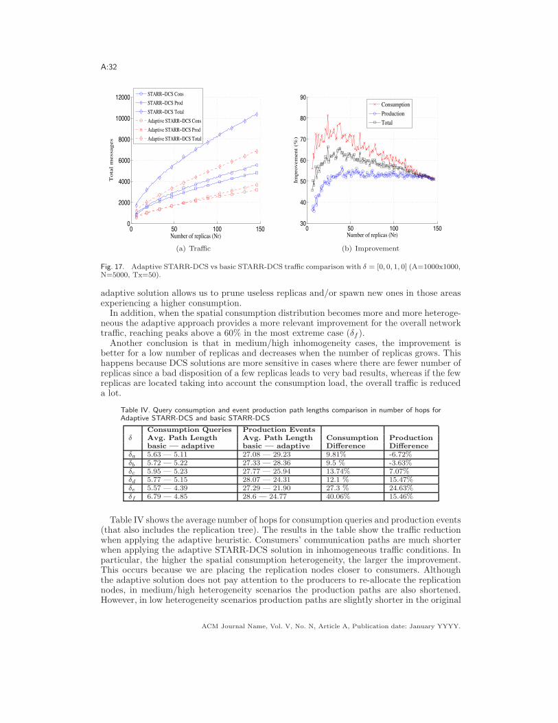
A:32

0 50 100 1500

2000

4000

6000

8000

10000

12000


Tot

al m

essa

ges

STARR DCS ConsSTARR DCS ProdSTARR DCS TotalAdaptive STARR DCS ConsAdaptive STARR DCS ProdAdaptive STARR DCS Total

(a) Tra!c

0 50 100 15030

40

50

60

70

80

90

Impr

ovem

ent (

%)



(b) Improvement

Fig. 17. Adaptive STARR-DCS vs basic STARR-DCS tra!c comparison with # = [0, 0, 1, 0] (A=1000x1000,N=5000, Tx=50).

adaptive solution allows us to prune useless replicas and/or spawn new ones in those areasexperiencing a higher consumption.

In addition, when the spatial consumption distribution becomes more and more heteroge-neous the adaptive approach provides a more relevant improvement for the overall networktra!c, reaching peaks above a 60% in the most extreme case (%f ).

Another conclusion is that in medium/high inhomogeneity cases, the improvement isbetter for a low number of replicas and decreases when the number of replicas grows. Thishappens because DCS solutions are more sensitive in cases where there are fewer number ofreplicas since a bad disposition of a few replicas leads to very bad results, whereas if the fewreplicas are located taking into account the consumption load, the overall tra!c is reduceda lot.

Table IV. Query consumption and event production path lengths comparison in number of hops forAdaptive STARR-DCS and basic STARR-DCS

Consumption Queries Production Events# Avg. Path Length Avg. Path Length Consumption Production

basic — adaptive basic — adaptive Di!erence Di!erence#a 5.63 — 5.11 27.08 — 29.23 9.81% -6.72%#b 5.72 — 5.22 27.33 — 28.36 9.5 % -3.63%#c 5.95 — 5.23 27.77 — 25.94 13.74% 7.07%#d 5.77 — 5.15 28.07 — 24.31 12.1 % 15.47%#e 5.57 — 4.39 27.29 — 21.90 27.3 % 24.63%#f 6.79 — 4.85 28.6 — 24.77 40.06% 15.46%

Table IV shows the average number of hops for consumption queries and production events(that also includes the replication tree). The results in the table show the tra!c reductionwhen applying the adaptive heuristic. Consumers’ communication paths are much shorterwhen applying the adaptive STARR-DCS solution in inhomogeneous tra!c conditions. Inparticular, the higher the spatial consumption heterogeneity, the larger the improvement.This occurs because we are placing the replication nodes closer to consumers. Althoughthe adaptive solution does not pay attention to the producers to re-allocate the replicationnodes, in medium/high heterogeneity scenarios the production paths are also shortened.However, in low heterogeneity scenarios production paths are slightly shorter in the original


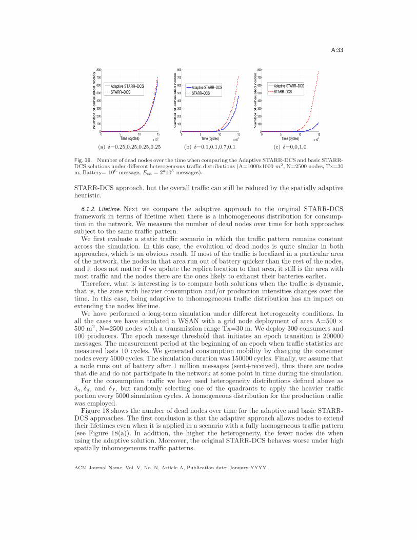
A:33

0 5 10 15x 104

0

100

200

300

400

500

600

700

800

Time (cycles)

Nu

mb

er

of

exh

au

ste

d n

od

es

Adaptive STARR DCSSTARR DCS

(a) #=0.25,0.25,0.25,0.25

0 5 10 15x 104

0

100

200

300

400

500

600

700

800

Time (cycles)

Nu

mb

er

of

exh

au

ste

d n

od

es


(b) #=0.1,0.1,0.7,0.1

0 5 10 15x 104

0

100

200

300

400

500

600

700

800

Time (cycles)

Nu

mb

er

of

exh

au

ste

d n

od

es


(c) #=0,0,1,0

Fig. 18. Number of dead nodes over the time when comparing the Adaptive STARR-DCS and basic STARR-DCS solutions under di"erent heterogeneous tra!c distributions (A=1000x1000 m2, N=2500 nodes, Tx=30m, Battery= 106 message, Eth = 2*105 messages).

STARR-DCS approach, but the overall tra!c can still be reduced by the spatially adaptiveheuristic.

6.1.2. Lifetime. Next we compare the adaptive approach to the original STARR-DCSframework in terms of lifetime when there is a inhomogeneous distribution for consump-tion in the network. We measure the number of dead nodes over time for both approachessubject to the same tra!c pattern.

We first evaluate a static tra!c scenario in which the tra!c pattern remains constantacross the simulation. In this case, the evolution of dead nodes is quite similar in bothapproaches, which is an obvious result. If most of the tra!c is localized in a particular areaof the network, the nodes in that area run out of battery quicker than the rest of the nodes,and it does not matter if we update the replica location to that area, it still is the area withmost tra!c and the nodes there are the ones likely to exhaust their batteries earlier.

Therefore, what is interesting is to compare both solutions when the tra!c is dynamic,that is, the zone with heavier consumption and/or production intensities changes over thetime. In this case, being adaptive to inhomogeneous tra!c distribution has an impact onextending the nodes lifetime.

We have performed a long-term simulation under di"erent heterogeneity conditions. Inall the cases we have simulated a WSAN with a grid node deployment of area A=500 )500 m2, N=2500 nodes with a transmission range Tx=30 m. We deploy 300 consumers and100 producers. The epoch message threshold that initiates an epoch transition is 200000messages. The measurement period at the beginning of an epoch when tra!c statistics aremeasured lasts 10 cycles. We generated consumption mobility by changing the consumernodes every 5000 cycles. The simulation duration was 150000 cycles. Finally, we assume thata node runs out of battery after 1 million messages (sent+received), thus there are nodesthat die and do not participate in the network at some point in time during the simulation.

For the consumption tra!c we have used heterogeneity distributions defined above as%a, %d, and %f , but randomly selecting one of the quadrants to apply the heavier tra!cportion every 5000 simulation cycles. A homogeneous distribution for the production tra!cwas employed.

Figure 18 shows the number of dead nodes over time for the adaptive and basic STARR-DCS approaches. The first conclusion is that the adaptive approach allows nodes to extendtheir lifetimes even when it is applied in a scenario with a fully homogeneous tra!c pattern(see Figure 18(a)). In addition, the higher the heterogeneity, the fewer nodes die whenusing the adaptive solution. Moreover, the original STARR-DCS behaves worse under highspatially inhomogeneous tra!c patterns.


A:34

Therefore, incorporating the sptailly adaptive heuristic to STARR-DCS does not onlyachieve better performance when there is a substantial tra!c heterogeneity, but it alsoextends nodes’ lifetimes under homogeneous conditions.

7. CONCLUSIONS

This paper demonstrates that static DCS systems are highly unfair in terms of energy con-sumption. Those nodes assigned with the role of home nodes and its surrounding neighbourswill naturally spend much more energy than other nodes in the network. Therefore, in or-der to extend the network lifetime is mandatory to fairly distribute the energy consumptionacross the network nodes. Then, this paper first demonstrates that placing multiple repli-cation nodes at random in a DCS system outperforms previous work in the literature basedon a single rendezvous point, grid-structured or uniform replication node placement. Fur-thermore, we have shown that equalizing the energy burdens across the network, by meansof changing the set of replication nodes over the time, achieves a huge improvement in theWSAN lifetime. These two conclusions have been validated in large WSANs by simulation,and a testbed with 20 motes. Finally, this work is the first to explore networks where eventsand queries generation are not homogeneous across the network. We have proposed a heuris-tic that e"ectively reduces the tra!c in the network and leads to use shorter communicationpaths.

REFERENCES

Ahn, J. and Krishnamachari, B. 2006. Fundamental scaling laws for energy-e!cient storage and queryingin wireless sensor networks. In MobiHoc ’06. ACM, New York, NY, USA, 334–343.

Ahn, J. and Krishnamachari, B. 2009. Scaling laws for data-centric storage and querying in wireless sensornetworks. IEEE/ACM Trans. Netw. 17, 4, 1242–1255.

Baccelli, F. and Bordenave, C. 2007. The radial spanning tree of a poisson point process. Annals ofApplied Probability 17, 305.

Baccelli, F., Klein, M., Lebourges, M., and Zuyev, S. 1997. Stochastic geometry and architecture ofcommunication networks. J. Telecommunication Systems 7, 209–227.

Baccelli, F. and Zuyev, S. 1996. Poisson-voronoi spanning trees with applications to the optimization ofcommunication networks. Operations Research 47, 619–631.

Baek, S. J. and de Veciana, G. 2007. Spatial model for energy burden balancing and data fusion in sensornetworks detecting bursty events. IEEE Trans. on Information Theory 53, 10, 3615–29.

Baek, S. J., de Veciana, G., and Su, X. 2004. Minimizing energy consumption in large-scale sensornetworks through distributed data compression and hierarchical aggregation. IEEE Journal on SelectedAreas of Communications 22, 6, 1130–1140.

Cuevas, A., Uruena, M., Romeral, R., and Larrabeiti, D. 2010. Data centric storage technologies:Analysis and enhancement. Sensors 10, 4, 3023–3056.

Dietrich, I. and Dressler, F. 2009. On the lifetime of wireless sensor networks. ACM Trans. Sen.Netw. 5, 1, 1–39.

Ee, C. T., Ratnasamy, S., and Shenker, S. 2006. Practical data-centric storage. In NSDI’06: Proceedingsof the 3rd conference on Networked Systems Design & Implementation. USENIX Association, Berkeley,CA, USA.

Jain, R. K., Chiu, D.-M. W., and Hawe, W. R. 1984. A quantitative measure of fairness and discrimi-nation for resource allocation in shared computer systems. Tech. rep., Digital Equipment Corporation.September.

Joung, Y.-J. and Huang, S.-H. 2008. Tug-of-war: An adaptive and cost-optimal data storage and querymechanism in wireless sensor networks. In DCOSS ’08: Proceedings of the 4th IEEE internationalconference on Distributed Computing in Sensor Systems. Springer-Verlag, Berlin, Heidelberg, 237–251.

Karp, B. and Kung, H. T. 2000. Gpsr: greedy perimeter stateless routing for wireless networks. In MobiCom’00. ACM, New York, NY, USA, 243–254.

Liao, W.-H., Shih, K.-P., and Wu, W.-C. 2010. A grid-based dynamic load balancing approach for data-centric storage in wireless sensor networks. Comput. Electr. Eng. 36, 1, 19–30.

Moller, J. 1994. Lectures on random Voronoi tesselations. Springer-Verlag.


A:35

Ratnasamy, S., Karp, B., Shenker, S., Estrin, D., Govindan, R., Yin, L., and Yu, F. 2003. Data-centricstorage in sensornets with ght, a geographic hash table. Mob. Netw. Appl. 8, 4, 427–442.

Ratnasamy, S., Karp, B., Yin, L., Yu, F., Estrin, D., Govindan, R., and Shenker, S. 2002. Ght: ageographic hash table for data-centric storage. In WSNA ’02: Proceedings of the 1st ACM internationalworkshop on Wireless sensor networks and applications. ACM, New York, NY, USA, 78–87.

Shenker, S., Ratnasamy, S., Karp, B., Govindan, R., and Estrin, D. 2003. Data-centric storage insensornets. SIGCOMM Comput. Commun. Rev. 33, 1, 137–142.

Stoyan, D., Kendall, W. S., and Mecke, J. 1995. Stochastic Geometry and its Applications. J. Wiley &Sons, Chichester.

Thang, N. L., Wei, Y., Xiaole, B., and Dong, X. 2006. A dynamic geographic hash table for data-centricstorage in sensor networks. In IEEE Wireless Communications and Networking Conference, 2006.WCNC 2006. IEEE, New York, NY, USA, 2168 – 2174.


a starr-dcs: spatio-temporal adaptation of …users.ece.utexas.edu/~gustavo/papers/de...

Documents