University of Nebraska at Omaha University of Nebraska at Omaha

DigitalCommons@UNO DigitalCommons@UNO

Student Work

11-1-2002

A Spatial Analysis of Crime for the City of Omaha A Spatial Analysis of Crime for the City of Omaha

Haifeng Zhang University of Nebraska at Omaha

Follow this and additional works at: https://digitalcommons.unomaha.edu/studentwork

Recommended Citation Recommended Citation Zhang, Haifeng, "A Spatial Analysis of Crime for the City of Omaha" (2002). Student Work. 2155. https://digitalcommons.unomaha.edu/studentwork/2155

This Thesis is brought to you for free and open access by DigitalCommons@UNO. It has been accepted for inclusion in Student Work by an authorized administrator of DigitalCommons@UNO. For more information, please contact unodigitalcommons@unomaha.edu.

A SPATIAL ANALYSIS OF CRIME

FOR THE CITY OF OMAHA

A Thesis

Presented to the

Department of Geography & Geology

and the Faculty of the Graduate College

University o f Nebraska

In Partial Fulfillment

of the Requirements for the Degree

Master of Arts

University of Nebraska at Omaha

By

Haifeng Zhang

November 2002

UMI Number: EP73697

All rights reserved

INFORMATION TO ALL USERS The quality of this reproduction is dependent upon the quality of the copy submitted.

In the unlikely event that the author did not send a complete manuscript and there are missing pages, these will be noted. Also, if material had to be removed,

a note will indicate the deletion.

DisswttltoH: PWbffishifti

UMI EP73697

Published by ProQuest LLC (2015). Copyright in the Dissertation held by the Author.

Microform Edition © ProQuest LLC.All rights reserved. This work is protected against

unauthorized copying under Title 17, United States Code

ProQuestProQuest LLC.

789 East Eisenhower Parkway P.O. Box 1346

Ann Arbor, Ml 48106 - 1346

THESIS ACCEPTANCE

Acceptance for the faculty of the Graduate College, University of Nebraska, in partial fulfillment of the

Requirements for the degree Master of Arts, University of Nebraska at Omaha

Committee

Name Department

p • ---- -

Mv A i jb o w lu -c

----~ C ̂ VvyyM/W\5

C hairperson iP - \ C .-" N

Pate... M.Qi/ .... ?lOOZ

A Spatial Analysis of Crime for the City of Omaha

ABSTRACT

Haifeng Zhang, M,A.

University of Nebraska, 2002

Advisor: Dr. Michael P. Peterson

The spatial patterns of four types of crimes (assault, robbery, auto-theft, and

burglary) and their relationships with the selected socio-economic characteristics for the

City of Omaha, Nebraska, were examined in this research. The crime data were based on

the 2000 police reported crime and the socio-economic data were extracted from the 1997

American Community Survey and land use data from the 2000 Omaha parcel file. The

location quotients of crimes (LQCs) were used to measure the relative specialization and

structure of crimes for each census tract, and as the dependent variables for the statistical

analysis. GIS techniques such as geocoding, spatial aggregation, and spatial analysis were

used for crime mapping and crime analysis. Factor analysis and multiple regression

models were employed to reveal the crime-causation relationships. Major findings of this

research include: (1) LQCs highlight the specialization of crime and can be effectively

used for GIS-based visualization and statistical analysis of crime; (2) the North Omaha

and the downtown areas (high-crime districts) have relatively higher occurrences of

violent crime and diversified structure of crimes while west Omaha (low crime districts)

has a relatively specialized crime structure that is dominated by property crimes; (3) a

modest proportion of the variance of crimes can be significantly explained by the

statistical models.

IV

Acknowledgement

First I want to express my thanks to the advisory committee members: Dr.

Michael P. Peterson, Dr. Charles R. Gildersleeve, and Dr. Dennis W. Roncek. Thanks a

lot for their invaluable guidance and instruction.

As my thesis advisor, Dr. Peterson consistently encouraged me and helped me

finish every part of this thesis. The right words in the right time directed me arrive at the

final destination. The accomplishment of this thesis contains his wisdom.

Dr. Gildersleeve, my graduate program advisor, helped me decide the thesis topic

and always gave me great support with his particular enthusiasm, so I can keep an

optimistic mind and overcome every obstacle during the tough process of work.

Dr. Roncek, a professor from the Department of Criminal Justice, suggested the

use of location quotients as the measure of crime variance and helped me decide the

demographic variables and the statistical models.

Thanks to Dr. Jihong (Solomon) Zhao, the Chinese professor from the

Department of Criminal Justice, and Dr. Weiguo Yin, a research assistant from the

Department of Physics. Both of them gave me a lot of instruction and help for revising

the statistical models./

Thanks to Laura Banker, my GIS lab class lecturer, who gave me valuable help

for figuring out how to do the grid cell analysis and other GIS techniques.

V

Special thanks to Lt. Don Trackenbrod, the police officer from the Omaha Police

Department, for providing me the most important thing for this research—the crime data.

Also, he enlightened me on the crime data recording and crime incidents geocoding.

Sincere thanks should be given to my TA colleagues: Kristi Demmel, Pavol

Hurbanek, Lesli M. Rawlings, and Mike Hauschild. Kristi provided me the 1990 census

tract file, the latest street file, and gave me very important suggestions on locating crime

incidents manually to increase the hit rate o f address matching. Lesli provided me the

Omaha zoning and parcel files and gave me insightful suggestions. Mike provided his

survey report on prevention of crime to me and told me a lot of useful information about

crime in Omaha. Pavol helped me figure out a lot of tough problems in data analyzing

and mapping.

Also, I need to express my gratitude to my parents, my wife, and all my friends

who gave me encouragement and support.

Finally, thank all the faculty and staff members in the Department of Geography

& Geology for their guidance, encouragement, and help. I really appreciate it.

vi

Table of Contents

List of Tables........................................................................................................... ix

List of Figures................................'.......................................................................... x

Chapter One INTRODUCTION........................................................................... 1

1.1. Nature of Problem................................................................................... 3

1.2. Objectives................................................................................................ 4

1.3. Hypotheses and Rationale....................................................................... 5

1.4. Study Area............................................................................................... 6

1.5. Significance of Research........................................................................ 8

1.6. Summary of Chapter............................................................................... 9

Chapter Two LITERATURE REVIEW .............................................................. 10

2.1 Introduction................................................................................................ 10

2.2 Theories on the Spatial Variation of Crime............................................ 10

2.3 Empirical Research...................................................................................; 13

2.4 Measures of Crime Occurrences. ......................................................... 18

2.5 GIS and Crime Analysis........................................................................... 20

2.6 Summary of Chapter................................................................................. 22

Chapter Three METHODOLOGY........................................................................ 24

3.1 Introduction................................................................................................ 24

3.2 Data Description.................................................................................... .. 24

vii

3.3 LQC as a Measure of Crime..................................................................... 31

3.4 GIS-Based Crime Analysis...................................................................... 32

3.5 Statistical Analysis................................................................................... 37

3.6 Summary of Chapter................................................................................ 40

Chapter Four RESULTS AND ANALYSIS........................................................ 42

4.1 Introduction............................................................................................... 42

4.2 Visualization of Crime with GIS............................................................. 42

4.3 Statistical Results and Analysis.............................................................. 63

4.4 Summary of Chapter................................................................................ 82

Chapter Five CONCLUSION................................................................................ 85

5.1 Overview of Thesis................................................................................... 85

5.2 Major Findings of Research..................................................................... 85

5.3 Future Work.............................................................................................. 88

References................................................................................................................... 90

Appendix

I-1: Crime data............................................................................... ................. 98

1-2: Socio-economic Data............................................................................... 101

1-3: Principal components of factor analysis............................................... 107

II: Fips of census tracts in Omaha, 1990 .......................................... 110

III-1: Map of Area for each census tract....................................................... I l l

III-2; Map of the total population for each tract........................................... I l l

III-3: Map of population density for each census tract................................. 112

viii

III-4: Population of young males at age of 15-24......................................... 112

III-5: Map of the percentage of African Americans..................................... 113

III-6: Map ofHispanics population.. . ........................................................... 113

TTT-7: Map o f unemployed dropouts at age of 16-19.................................... 114

III-8: Map of the adults without high school diploma................................. , 114

III-9: Map of female-headed households...................................................... 115

III-10: Population living in housing with 1.01 or more per room............... 115

TTT-11: Median household income................................................................ 116

III-12: Median house value........................................................................... 116

III-13: Map of percentage of unemployment.............................................. 117

III-14: Percentage of people with income below poverty.......................... 117

III-15: Map of owner-occupied houses........................................................ 118

III-16: Percentage of vacant houses.............................................................. 118

III-17: Percentage of persons who live in the same house over 5 years 119

III-18: Percentage of multifamily parcels...................................................... 119

III-19: Percentage of commercial parcels...................................................... 120

ix

List of Tables

Table

1.1 Crime incidents in Omaha, 2000.......................................................... 7

3.1 List of dependent and independent variables...................................... 29

4.1 Geocoding results of crimes.................................................................. 43

4.2 Count and LQCs in example census tracts......................................... 57

4.3 Descriptive statistics of dependent variables...................................... 65

4.4 Correlation matrix of independent variables....................................... 66

4.5 Regression summary of Model-1.......................................................... 68

4.6 Regression summary of Model-2.......................................................... 69

4.7 Total variance explained by principal components............................ 73

4.8 Principal components from factor analysis......................................... 74

4.9 Regression summary of Model-3.......................................................... 76

4.10 Regression summary of Model-4........................................................ 78

X

List of Figures

Figure

3.1 Methodological design of crime analysis in Omaha.................... 25

3.2 Census tract map of Omaha, 1990. ............................................... 27

4.1 Assault crime incidents in Omaha, 2000....................................... 45

4.2 Robbery crime incidents in Omaha, 2000..................................... 46

4.3 Auto-theft crime incidents in Omaha, 2000............................ 47

4.4 Burglary crime incidents in Omaha, 20000................................. 48

4.5 Multifamily & commercial parcels and robberies.................... 49

4.6 Multifamily & commercial parcels and assaults ................... 50

4.7 Map of commercial parcels and auto-thefts............................ 51

4.8 Assault density in Omaha, 2000................................................... 53

4.9 Robbery density in Omaha, 2000............................ 53

4.10 Auto-theft density in Omaha, 2000......................................... 54

4.11 Burglary density in Omaha, 2000............................................. 54

4.12 Location quotient of assault crime in Omaha, 2000................ 58

4.13 Location quotient of robbery crime in Omaha, 2000................ 58

4.14 Location quotient of auto-theft crime in Omaha, 2000............ 59

4.15 Location quotient of burglary crime in Omaha, 2000........... 59

4.16 Map of the crime structure for each tract, 2000............ .. .,.... 60

4.17 Count of assault crime in Omaha, 2000. .................................. 61

xi

4.18 Count of robbery crime in Omaha, 2000.................................. 62

4.19 Count of auto-theft crime in Omaha, 2000................................. 62

4.20 Count of burglary crime in Omaha, 2000................................. 63

1

Chapter One

INTRODUCTION

Crime is one of America's top domestic concerns. The research on the

geographical distribution and the search for explanations of the spatial variations in crime

has long been a prominent area o f analysis for both researchers and practitioners.

Criminologists and sociologists believe that crime is a reflection of antisocial

aggression and influenced by regional socio-economic characteristics (Reith, 1996).

From the perspective o f spatial analysis, geographic studies suggest that crime has a

geographic dimension and is disproportionately distributed across various spatial units —

from neighborhoods and cities to regions, nations, and the global scale. In city and

metropolitan areas, crime is highly concentrated in relatively few, small areas. U.S

criminal statistics show that the percentage of population living in cities and metropolitan

areas is 75 percent, but more than 95 percent of all crimes occurred in urban areas

(Ousey, 2000). A quantitative study made by Sherman et al. (1989) finds that 3.3 percent

of street addresses and intersections in Minneapolis were responsible for 50.4 percent of

all dispatched police calls for service. Similar patterns of crime are also found in other

cities (Pierce et al., 1988; Sherman, 1992; and Weisburd and Green, 1994). Researchers

also find that urban crime occurs most frequently in stressful and disadvantaged areas,

and socio-economic factors, such as poverty, income inequality, unemployment, over­

crowding, racial heterogeneity, youth concentration, and environmental risks, etc. are the

most important contributors of crime distribution (Garrett, 1995).

2

Statistical analysis methods such as factor analysis and multiple regression

models have long been utilized in the analysis of crime. Factor analysis is an effective

approach in crime causation analysis to abstract the major underlying independent

components (Tachovsky, 1983; Acherman, 1998; Krivo and Peterson, 1996). Taking the

occurrence of crime, such as crime rate or count, as the dependant variable, the selected

socio-economic attributes as the independent variables, regression analysis plays a

critical role in the explanation of the causation of criminal activities (Anselin, et al.,

2000).

Choosing different measures of crime may result in a different profile of crime for

a region and directly affect the results of statistical analysis. The most important concern

for crime analysis is to select appropriate indicators to measure the crime occurrence.

Conventional measurements such as crime rate or count of crime are commonly used by

researchers to indicate the level of crime activity across areas. Though popular, there are

limitations for these two indicators. For example, they are often affected by the

population size and density and may result in biased conclusions (Brantingham and

Brantingham 1995; Carcach and Muscat 2002). Beyond these limitations, the location

quotient was incorporated into crime analysis to evaluate the relative concentration or

specialization (compared to the larger reference area) of specific crime for certain areas

in recent years.

Historically, crime mapping is a significant aspect of crime control and crime

analysis. The recent advance of computer mapping and GIS techniques accompanied by

the development of spatial analysis methods has greatly enhanced our understanding of

3

the dynamics of crime (Carcach and Muscat, 2000). Compared with the conventional

statistical methods, geographical information systems (GIS) provides the added potential

for linking criminal incidents with geographic locations and graphically displaying the

spatial relationship between crime and the socio-economic factors. There are dozens of

analysis methods for displaying the crime distribution and the correlated socio-economic

characteristics. These techniques range from simple point map to three-dimensional

density displays. More advanced use of GIS technology involves overlaying crime

incident maps with other socio-economic features to explore the correlation with high

crime concentrations and variation over space (Gisela and Johnson, 2001). GIS is not

only instrumental in helping society to visualize the linkages between crime and socio­

economic stress factors within an area, but also is beneficial for the public to cooperate

with the law enforcement agencies to trim down the stress level and prevent the

occurrence of crime in their neighborhoods and the whole city (Murray, et. al. 2001).

1.1 Nature of the Problem

In people's general perception, crime in Omaha occurs more frequently in the

eastern part, generally east of 72nd street, while west Omaha is almost free from crime.

The Omaha World-Herald released a special report of Omaha crime based on seven and

half years of crime data. Their conclusion:

“... The east-west (divided by the 72nd Street) perception oversimplifies crime’s impact on Omaha. While crime is more prevalent in the east, the most common crime — theft - invades every part o f the city. ... Crime is concentrated most in the northeast area, particularly from Cuming Street to Ames Avenue, between the Missouri River and 48th Street. The northeast suffers from high unemployment, a lower median income and more decaying infrastructure than the rest o f the city. The area is home to many o f the city’s poor and African-Americans....” (Napolitano, 1998)

4

This report also indicates that socio-economic characteristics are important but

not the only factors related to the occurrence of crimes across neighborhoods. Other

issues such as access to large shopping centers, apartment complexes, interstate

highways, and major roads also have important links to crime. While the World-Herald

report provides very detailed descriptive picture of crime and useful information for the

public in Omaha, it lacks statistical analysis to support its claims.

Except for the Omaha World-Herald’s descriptive survey, there is little research

on the systematic analysis of spatial differentiation and the causation of crime for the City

of Omaha. To further examine the distribution pattern and explore the underlying major

correlates of crime variance across neighborhoods of Omaha, an in-depth empirical

analysis integrating advanced GIS techniques and statistical models was undertaken for

this research.

1.2 Objectives

Reported crime data for the year of 2000, including assault, robbery, auto-theft,

and burglary were collected for analysis. The purpose of this research was to display the

distribution patterns of the four types of crimes and explore the relationship between the

selected socio-economic characteristics and land use with crimes in the City of Omaha.

Specifically the objectives include:

• Examining the spatial variation of crime using the GIS techniques of

address matching, spatial aggregation, and spatial analysis;

• Using the location quotients to measure the specialization and structure of

crimes and as dependent variables to conduct the statistical analysis.

5

• Comparing the statistical predictability of location quotient models with

the model using conventional measure (count of crime) for identifying the

effects of the selected socio-economic characteristics on the spatial

variations of crimes across census tracts.

1.3 Hypotheses and Rationale

Three hypotheses tested by this research:

First, crime is disproportionately distributed in the City of Omaha. GIS techniques

can be employed to display the spatial distribution pattern of crime across the city.

Second, LQC as an alternative measure of crime rate can be effectively used for

mapping the specialization and structure of crimes and used as dependent variables for

the regression analysis in explaining the effects of the selected socio-economic variables.

Third, the spatial differentiation of the assault, robbery, auto-theft, and burglary

can be statistically explained to a significant degree by the selected socio-economic

characteristics. Specifically, social stress variables such as percentage of African

American, percentage of Hispanics, female-headed households, poverty, vacant house,

and unemployment rate are thought to be positively correlated with the occurrence of

crimes, while other variables such as house ownership and median house income (or

house value) should have negative relationships with crime. In addition, the land use

patterns, such as multifamily and commercial parcels are also hypothesized to exert

positive contribution to the occurrence of crime.

The rationale that underlies this research is based on the following three points.

First, this research is based on the two predominant crime theories: social disorganization

6

theory and the routine activity theory, and previous researchers have provided sufficient

support of empirical research on these two theories. Both social disorganization and

routine activity theories were used to select explanatory indicators for this research.

Second, most of the independent variables in this research have been widely used and

found to have statistically significant associations with the spatial variation of urban

crime. Third, LQC is one of the most extensively used indices to assess the relative

specialization of local economic activities, and has been applied for crime analysis by

previous researchers. Carcach and Muscat (2002) have examined the statistical

properties of location quotient and conclude that it can be used as the dependent variable

for statistical analysis o f crime.

1.4 Study Area

The study area of this research is the City of Omaha. The Omaha metropolitan

area enjoys a reputation as one of the safest midsize cities in the United States. The City

of Omaha is the major part o f the metropolitan area and has 54.4 percent of the total

population. In 2000, the crime rate of all categories of crimes in Omaha was 5,319.2 per

100,000 population. According to the 2000 FBI Uniform Crime Report, Omaha ranked in

the lowest quartile in violent crime rate of the 276 cities surveyed in the United States.

However, crime is still one of the major concerns for the people of Omaha.

According to the results of Omaha Conditions Survey (1990) on the fear of crime:

... 91.5 percent of the respondents in Omaha were worried about crime. 47 percent were very worried about crime. Especially, nonwhite and female respondents were most worried about crime (Marshall, 1990).

7

A recent poll on crime conducted by Omaha World-Herald in 1998 reinforced the

conclusion above and found that approximately half of the residents surveyed worried

about being victims of crime (Napolitano, 1998). From the results of these two surveys, it

is apparent that the study of the spatial variation of crime in Omaha is important to

analyze. The research can also help citizens of Omaha to better understand the spatial

pattern of crime, so that they do not have unreasonable fears.

The 2000 crime data collected from the Omaha Police Department provide the

basic information of crime incidents in the city. The original data file includes seven

kinds of crimes including homicide, assault, robbery, larceny, auto-theft, burglary, and

misdemeanor (Table 1.1). Though not identical with the Uniform Crime Report, it is an

accurate representation of crimes committed in Omaha. In this research, assault, robbery,

auto-theft, and burglary, which represent the general profile of crime in Omaha and are of

concern to the police and public, were selected for the crime mapping and statistical

analysis.

Table 1.1 Crime incidents in Omaha, 2000

CrimeType

Homicide Assault Robbery Larceny Auto­theft

Burglary Mis-Demeanor

Counts 23 591 855 16490 3923 3267 1103

Source: Omaha City Police Department, 2000.

8

1.5 Significance of Research

Combining the current GIS techniques and statistical analysis methods, this

research provides very important reference for both geographers and criminologists.

Specifically, from the perspective of spatial analysis of crime, the significance of this

research lies in four aspects:

• Firstly, it provides a better understanding of the geographical differentiation of

crime in the City of Omaha;

• Secondly, the results of this research have implications for testing the social

disorganization and routine activity theories of crime variation;

• Thirdly, it sheds light on the crime mapping and statistical analysis of crime by

using location quotients as an alternative measure to reveal the specialization and

structure of crimes across census tracts;

• Finally, it is beneficial for law enforcement and the public to visualize the

distribution patterns of crime and its linkage to socio-economic characteristics.

Therefore, it is helpful for the prevention of potential crimes.

Because location quotients can highlight the relative concentration of different types

of crimes across census areas, this research will greatly help police department take

effective measures to tackle present crimes and prevent potential offenses in different

neighborhoods. Also, using location quotients is potentially helpful in studying fear of

concern about crime. This research is informative for addressing people’s unreasonable

worries of crime and answering public questions such as: “Where is the highest risk area

for a certain type of crime?” “What’s the dominant crime type in a certain area?” and

9

“Which characteristics account for the occurrence of a specific type of crime being high

in this area?”

1.6 Summary of Chapter

Both criminologists and geographers have long emphasized research on the

spatial distribution and the underlying causes for the variation of crime. Utilizing GIS

techniques and statistical analysis methods, this research aims to reveal the spatial pattern

o f crime and explore the relationship between socio-economic characteristics and crime

across census tracts in the City of Omaha. The major hypothesis is that the selected socio­

economic and land use indicators can significantly explain the variation of crime.

The remainder of the thesis is divided into four major sections. Chapter Two

reviews the literature in both theoretical and empirical research in the spatial variation of

crime, the measures of crime, crime mapping, and statistical analysis of crime. Chapter

Three provides the framework designed to comprehensively depict the picture o f crime

and statistically analyze the crime-causation relationships. Chapter Four presents the

results of the crime mapping and statistical analysis. The last chapter is the conclusion of

this research discussing the major findings and potential for future work.

10

Chapter Two

LITERATURE REVIEW

2.1 Introduction

The analysis o f the geographical patterns of crime can be traced back to the work

of two French social ecologists and statisticians Guerry and Quetelet during the middle of

frVi • *19 century, who first declared that crime incidents were distributed unevenly across

geographic space (Anselin et al., 2000). In the United States, it was H. V. Redfield (1880)

who did a pioneer work on studying the spatial distribution of crime and found that the

southern states experienced higher crime rates than the rest of the country. The Chicago

School in the early 20th century opened the American history of sociological research in

crime by conducting an investigation of juvenile crime across community areas for

Chicago. Since the 1960’s, the geographical focus of crime analysis had shifted from

regional areas to city neighborhoods (Ousey, 2000).

2.2 Theories on the Spatial Variation of Crime

Sociologists and criminologists focusing on spatial variation of crime at the

community level have offered several explanations for the fact that crime rates are highly

concentrated in stressful and disadvantaged neighborhoods. The dominant explanation

derives from Shaw and McKay’s (1942) social disorganization theory, which was

reinterpreted and developed by subsequent researchers. The main points of this theory

are that the socio-economic stress factors will ultimately reduce the level of social control

and result in the disruption of community social organization, which in sequence

accounts for high crime and delinquency rates (Agnew 1999, Ackerman, 1998). Other

11

similar theories that proposed to explain community crime differences include the social

stratification (or structure) theory, subculture theory, absolute and relative deprivation

theory, and general strain theory. The commonality o f these theories is that either socio­

economic stress, or culture or social strain is the major source of criminal motivation.

The social disorganization theory was suggested by several empirical studies

(e.g., Bellair 1997; Sampson and Groves 1989; Sampson et al. 1997). Despite being

broadly exploited in the analysis of urban crime, however, the weakness of social

disorganization theory is that it implicitly assumes that plentiful opportunities to commit

crime are always available, and those who are disadvantaged are supposed to be more

prone to commit a crime (Rice and Smith, 2002). Critics of this theory argue that social

disorganization theory reinforces the “class bias” or racial discrimination and cannot

explain the occurrence of crimes in “stable” and “organized” wealthy districts in the

urban areas. They also argue that there is a failure for social disorganization theory to

explain the deviation between the spatial distribution of offenders and the distribution of

crime incidents (criminals do not necessarily commit crime in the area where they live)

(Herbert, 1980). Though flaws exist, social disorganization still draws attention and is

further developed by recent researchers by incorporating “social network” and

“community attachment” into the disorganization model to mediate the role of the socio­

economic stress factors in shaping the profile of community crime (Bursik 1988; Kasarda

and Janowitz, 1974; Ousey, 2000; Sampson 1987; Warner and Rountree 1997)

Another major theory for explaining the distribution of crime is routine activity

theory. First introduced by Cohen and Felson (1979), the routine activity approach

12

claims that criminal incidence and victimization are related to the environment and

behavior patterns of people. Three key elements are indispensable for the occurrence of

crime: desirable targets, motivated offenders, and absence of capable guardianship

(Sherman and Burger, 1989). In a review paper, Anselin et al. (2000) states:

"... The distribution o f crime is determined by the intersection in time and space o f suitable targets and motivated offenders. ...Routine activities that bring together potential offenders and criminal opportunities are especially effective in explaining the role o f place in encouraging or inhibiting crime. The resulting crime locales often take the form offacilities — places that people frequent fo r a specific purpose — that are attractive to offenders or conductive to offending. (Criminal Justice 2000, Vol. 4, pp 213-235)

From the viewpoint of routine activity theory, crimes most frequently occur at

places where abundant opportunities are available for the most profitable crime and the

least chances of surveillance or capture. Empirical research based on the routine activity

theory finds that land use and environmental conditions are important indicators for

diagnosing the hot spots of crime concentration. Locations with “target-rich

environments” such as 24-hour stores, large parking lots, and bars are frequently plagued

by varieties of crimes (Anselin et al.j 2000; Roncek and Maier, 1991).

Social disorganization theory and the routine activity approach share some

common points: such as (1) both theories stress the role of social control in reducing the

occurrences of crime in communities; and (2) they also have similar assumptions on the

motivation of the offense, however they focus on a different scale of in the spatial aspect

of crimes (Rice and Smith, 2002). While social disorganization theory explains the spatial

variance of crime from the macro scale (i.e., ‘the nested neighborhood5) (Slovak 1986),

routine activity theory attempts to account for the association between crime and the

13

specific places from the micro level (i.e., ‘the immediate visible environment surrounding

a potential crime event’) (Rice and Smith, 2002). Therefore, when analyzing the spatial

distribution pattern (both areal and hot spot analysis) o f urban crime, it is necessary to

integrate these two theories. Actually, some theorists and researchers have proposed that

social disorganization and routine activity theories are “complementary” and a

“combined model” may be more effective in accounting for the crime variance across

space (Bursik and Webb, 1982; Miethe and Meier 1994; Rice and Smith, 2002).

In general, although many different views have been proposed to explore the

causation of spatial divergence of crime, in fact, different theories shed light on different

aspects of the crime activity and are only suited for the explanation of certain types of

crimes. From this point, all theories are partially valid and have respective limitations.

Agnew (1999) notes that a satisfactory explanation of community differences in crime

rates needs to integrate a range of theories covering both the stimulation and control

perspectives of community crime. In this research, both social disorganization and

routine activity theories are used to guide the map interpretation and statistical analysis of

crimes.

2.3 Empirical Research

Empirical studies involving socio-economic correlates of crime on the aggregate

levels have always tried to find a link between the social-economic factors and crime to

test the above theories. A large body of research by geographers and other social

scientists has generated considerable supporting evidence on the distribution and spatial

dynamics of metropolitan and neighborhoods crime (Ackerman, 1998; Beasley and

14

Antunes, 1974; Harries, 1994; Kohfeld and Sprague, 1988; Krivo and Peterson, 1996;

Roncek and Meier, 1991; Weatherbum and Lind, 1997 and 2001). Factor analysis,

correlation, and regression models are frequently used to explore the relationship between

stress factors and crimes. Factor analysis can transform a collection of large, highly

correlated explanatory variables into fewer principal factors and keep as much predictive

power as the original indicators regarding the dependent variable. It has been widely

employed in socio-economic research for data reduction and handling severe

multicollinearity in multiple regression models. Using the occurrence of crime as the

dependent variable and demographic variables as the independent variables, regression

analysis plays a crucial role in the attempts to explain the causes of criminal activities

(Anselin et al., 2001).

Beasley and Antunes (1974) analyze the determinants of crime for Houston,

Texas, and use predictor variables, including median income, median value of owner

occupied homes, population density, and percentage of African Americans, for the

regression analysis with data aggregated to twenty police districts in the city. After a

series of regression analyses (i.e., bivariate, multiple linear, polynomial, and special

regression models), they conclude that the selected variables can statistically explain

almost all of the variance in the rates of major crimes (85 percent for the personal crime,

and about two-thirds for the property crime) that they examined. They also suggest that

social stress and the potential economic profit account for the variation of personal or

violent crime and property crime respectively.

15

Tachovsky (1983) uses factor analysis and correlation analysis to investigate the

relationship between selected socio-economic characteristics and the observed patterns of

crime rates in New Castle County, Delaware. Eighteen-month time series data on

nineteen crime components were selected for 107 census tracts, which serves as the basic

unit for statistical analysis. Factor analysis is used to extract both the major crime

dimensions and the principle components of socio-economic variables respectively. The

major finding of Tachovsky (1983) is that more than 50 percent of all criminal offenses

can be statistically explained, and the canonical model was more successful in delineating

and predicting the property crime than the violent crime.

Recent statistical analysis include: Krivo and Peterson’s (1996) case study that

uses census tract data in the city of Columbus, Ohio, and shows that disadvantaged

communities have qualitatively higher levels of crime than less disadvantaged areas, and

that this pattern is evident for both black and white communities. This research suggests

that census tracts are the “best local areas” considering the data availability for crime

analysis and have been successfully used by former researchers. Also, they use three

years (1989-1991) average data of crime to reduce the annual fluctuations and permit

including crime incidents in tracts where crime does not occur every year.

Ackerman (1998) employs factor analysis and step-wise regression models to

analyze the crime differentials between 111 smaller communities in Ohio. Seven index

crimes of murder, rape, robbery, aggravated assault, burglary, larceny, and auto-theft

were gathered from the FBI’s Uniform Crime Report for the years 1976 through 1994.

Fourteen socio-economic variables were selected to evaluate the social stress gradients of

16

different cities. After the factor analysis, four principal components (race/weak family

structure, economic marginalization, human capital deficiency, and youth) were

abstracted and used as the independent variables for the later regression analysis. Finally,

the statistical results indicate that crime is primarily related to the concentration of

minorities, female headed households, poverty, unemployment, population, vacated

house, education deficiency, and high ratio of young people. Also, this research exhibits

that while race and weak family structure contribute more in explaining the violent crime

variation than economic marginalization, population size, human capital deficiency and

youth, property crime is most closely related with poverty and disadvantaged

neighborhoods than race and weak family structure. These findings are consistent with

theoretical expectations and with former empirical results from studies of metropolitan

areas. Yet, the problem is that only half of the variation of crime rates can be explained

by the selected socioeconomic and demographic factors.

Weatherbum and Lind (2001) use the census data based on postcode level and the

linear regression models to determine, which combination of the measures of social and

economic stress (poverty, unemployment, stability, single parent families and crowded

dwellings) will be most effective in explaining juvenile participation in crime in New

South Wales, Australia. This research concludes that poverty, single parent families, and

crowded dwellings are the most important stress predictors of juvenile delinquency. On

the contrary, neither unemployment nor stability is necessary in predicting juvenile

participation in crime.

17

Based on the integration of social disorganization and routine activity theory, Rice

and Smith (2002) study the variation of auto-theft crime across face blocks (both sides of

a street at the block level) for a southeastern U.S city with a population about 250,000.

They select both social disorganization variables (including low building value, African

Americans, racial heterogeneity, single parent families, and distance from city center) and

routine activity variables (including apartment value, number of vacant houses, number

of parking lots, number of commercial places, etc), and including an automobile potential

to control for spatial autocorrelation. The results demonstrate that the integration of both

the social disorganization and routine activity theory can better explain the variance of

auto-theft crime.

Researchers have developed a large inventory of social and demographic factors

to account for the areal differentiation of crime, such as poverty, inequality, overcrowded

neighborhoods, unemployment, transient, racial heterogeneity, youth, land uses, and the

number of commercial facilities (Ackerman, 1998; Beasley and Antunes, 1974; Carcach

and Muscat, 2002; Glaeser et al., 1996; Rice and Smith, 2002; Roncek and Maier, 1991;

Tackovosky, 1983; Weatherbum and Lind, 2000; Zhao and Thurman, 2001).

In general, while a majority of crime studies found a positive link between social

stress and urban crime, others failed to produce a significant finding. In addition, some

studies have found evidence of an inverse association between crime correlates (such as

unemployment and income inequality) and crime (Chiricos, 1987; Belknap, 1989).

Review papers by Weatherbum and Lind (2001) and Box (1987) suggest that the pattern

of empirical test results appears to depend on the time period, the data type of crime

18

(offenders, victims, or incidences), the data source (Uniform Crime report data or self-

reported data), the sample size and the methodology (time series or cross-sectional

analysis) employed for the explanation of the social stress-crime relationship.

2.4 Measures of Crime Occurrences

To represent the crime pattern accurately, special caution is needed for the

selection of crime measures, such as counts of incidents, crime rates, etc. Utilizing

different measurements can produce different conclusions about the level of crime in

areas and lead to different results when comparing the crime variation across geographic

areas and conducting statistical analysis (Carcach and Muscat, 2000). While most o f the

previous studies use crime rates or counts of crime to assess the crime occurrence and

perform statistical analysis, there exist some problems with the employment of crude

incident counts and crime rates for regional comparisons. This is because both the

absolute crime count and the population based crime rate can produce a misleading

profile of the spatial pattern of crime due to variations of population size and density in

the regions (Carcach and Muscat, 2000). For example, using counts of incidents cannot

reflect the difference between two areas with the same number of crimes but with

different areal size. Crime rates for peripheral areas of the city may be exaggerated

because the small size of population. On the contrary, crime rate in the densely populated

areas may be underestimated.

For these reasons, it is important to employ alternative indicators to eliminate the

bias of the conventional measures. The location quotient, a relative indicator that has

been commonly used in geographical, regional science and regional planning research, is

19

extended to the field of crime mapping and statistical analysis (Brantingham and

Brantingham, 1995; Carcach and Muscat, 2000 and 2002). Brantingham and

Brantingham (1995) did pioneering work by using the location quotients of crimes

(LQCs) to study the hot spots of crime in Canadian cities and confirmed that LQCs could

be employed to understand how one area is different from another in crime structure and

concentration. LQCs compare the relative share of a certain kinds of crime in a small

area to the total of this kind of crime in the bigger area and help identify whether a

specific crime pattern is disproportionately high or low in a particular place regardless of

the area’s total amount of crimes or population (Carcach and Muscat, 2002).

Lu (2000) investigates the pros and cons of different point pattern analysis

methods of crime and concludes that the location quotient has the unique advantage for

revealing the specialization pattern across areas over other techniques (such as pin map,

cluster analysis, and kennel density). Carcach and Muscat (2002) extends the previous

research on the general fields of location quotients and examines on the exploitation of

the “statistical properties” of LQCs. They claim that LQCs follow a multivariate log­

normal distribution and can be used for standard statistical procedures to examine the

influence of socio-economic disadvantage over LQCs. Their case study for the

Wollongong and the Blue Mountains (Sydney, Australia) uses location quotients of

different crimes (i.e., robbery, assault, residential burglary, non residential burglary,

vehicle theft, drug offenses, etc,) for each postal area as the dependent variables and uses

the census characteristics of corresponding area units as the predictor variables in a

multiple regression model. The general conclusion from this analysis is that socio­

20

economic characteristics are the main factor in shaping the crime profiles o f postal areas

of Wollongong and the Blue Mountains in Sydney, Australia.

2.5 GIS and Crime Analysis

Using maps to display the spatial pattern of crime and the risk determinants has

long been an indispensable part of the crime mapping and crime analysis (Harries, 1999).

After the mid-1960s, computer-mapping techniques were broadly used for mapping

crime occurrence. In the last twenty years, with the integrated functions of database

management, spatial analysis and visualization, GIS has emerged as an outstanding

instrument in crime mapping and spatial analysis for both researchers and practitioners.

Graphically displaying the spatial distribution and associated socio-economic

characteristics and allowing the examination of the spatial relationship between crime

and the associated demographic factors are the distinctive advantage of GIS.

Harries (1994) examines the spatial relationships between juvenile gun crime and

social stress in Baltimore 1980-1990 using GIS techniques. He first geocoded the 2,639

juvenile gun crimes on the map and developed a social stress index comprising the

percent black, percent under age of 18, persons per occupied housing units, percent

female and median home value at the census tract level. Then, GIS spatial analysis is

used to overlay the census tract, the social stress indices, and the crime data layers to

assess the relationships between social stress, selected demographic attributes and the

distribution of gun crimes. Finally, Harries concludes: (1) African-American youths were

heavily over-represented in the commission of gun crimes; (2) there exists a general

spatial association between high social stress and high frequencies of crime incidents

21

over the 11-year period. In the guidebook “Mapping Crime: Principle and Practice”,

Harries presents a systematic exposition of the principles and techniques of GIS and

includes more than 110 maps to illustrate how GIS works in the application of crime

mapping and analysis. Murray et al. (2001) discuss the application of GIS and

quantitative techniques for better understanding the relationships of crime occurrence in

Brisbane, Australia. This research lists the detailed approaches of GIS capabilities, such

as proximity analysis, spatial containment, scatter-plot map and cluster analysis for the

analysis of crime in urban regions. Lu (2000) portrays the picture of hot spots of the

unauthorized use of vehicles using location quotients as measure of crime occurrence for

the City of Buffalo, NY in 1996.

Brimicombe et al. (2001) integrate statistical analysis and GIS techniques to

identify the contribution of neighborhood effects to the rate of allegations of racist crimes

and harassment in the Borough of Newham, London. GIS plays an important role in

finding further possible predictor variables by creating a range of map visualizations of

racial incidents against demographic variables.

Generally, the major applications of GIS in crime can be integrated into five

aspects:

• Relative ease of displaying crime incidents and socio-economic factors on maps;

• Permitting flexible measurements at various levels of spatial aggregation (Anselin

et al., 2000);

• Capability to integrate crime statistics with census and other spatial dimensions

(Murray et al. 2001; Anselin et al, 2000);

22

• Operating spatial analysis, such as density analysis, proximity analysis, and

neighborhood analysis, etc;

• Performing spatial statistical analysis and the mapping of the geographical

distribution of the statistical results.

2.6 Summary of Chapter

The leading theories on the causes of crime variation across communities,

empirical analysis, the measurement of crime, and GIS visualization of crime were

reviewed in this chapter separately. The following points need to be highlighted for

constructing the methodology of this research:

• Social disorganization and routine activity are the two most predominant theories

in explaining the spatial variation of urban crime. These two theories are

complementary and can be integrated to account for the distribution pattern of

crime across urban areas.

• Factor analysis and regression models have been commonly used in abstracting

the principal components of socio-economic characteristics and evaluating the

crime-causation relationship.

• Independent variables reflecting social disorganization and routine characteristics,

including poverty level, female or single headed households, unemployment rate,

racial heterogeneity, education deficiency; multi-family housing, vacant houses,

instability or transient, commercial places, and entertainment places, are

frequently selected and have been proven as satisfactory predictors of crime

occurrence.

23

• Choosing appropriate crime indicators is important for crime mapping and

statistical analysis. Compared with the crime rate and the count of incidents, the

LQC possesses distinctive advantages for analyzing the local concentration of

crime and in comparing crime specialization over time and space.

• GIS is not only an important tool for mapping the distribution of crime, but GIS

may also be able to enhance, supplement and extend the traditional quantitative

techniques in spatial analysis of crime, such as the techniques of density analysis

and the visualization of results of regression models (Murray et al., 2001).

In general, although there is enormous previous literature on spatial and statistical

analysis methods to delineate the distribution pattern of crime and explaining the

causation for spatial variation of crime, little emphasis has been put on integrating GIS

techniques and statistical analysis to portray the spatial pattern and explore the internal

mechanism of crime-causation relationship, particularly employing location quotients as

the measurement of crime specialization to conduct the crime mapping and statistical

analysis across census tracts within a city. Based on this point, this thesis aims to

combine the GIS visualization functions and statistical analysis methods to depict the

profile of the geographical distribution and causation of crime for the City of Omaha.

24

Chapter Three

METHODOLOGY

3.1 Introduction

This chapter presents the methodology to analyze the data and test the hypotheses.

The major procedures for performing the GIS visualization and statistical analysis of

crimes for the City of Omaha are displayed in Figure 3.1. The justification and

explanation of the methodological design including data description, measurement

choice, GIS visualization, and statistical analysis models are described in this chapter.

3.2 Data Description

Data for this research were gathered from three principal sources: (1) Crime data

from the Omaha City Police Department, and (2) Demographic data from the 1997

American Community Survey; (3) the land use parcel file from the Omaha City Planning

Department. The reason for using community survey data instead of the 2000 census data

is that the 2000 Census attributes were not available when this study began. In addition, it

is important that the demographic data precede the crime data for analyzing the causation

of crime. Other digital data required for the mapping of crime includes the Omaha street

shape file and the 1990 census tract shape file. To investigate the spatial patterns of crime

and examine the statistical relationship between crime and socio-economic variables, a

geo-referenced dataset was compiled at the census tract level for the study area.

25

Demographic & Land UseCrime Data

VariableExtraction

AddressMatching

FactorAnalysis

Aggregation

Dependent IndependentVariables Variables

MultipleRegression

Analysis

GIS-Based Crime Mapping

Crime Analysis

A Spatial Analysis of Crime for the City of

Omaha

Figure 3.1 Methodological design of crime analysis in Omaha

26

The census tract is the most appropriate areal unit for which the required socio­

economic data are available, and has been used by previous research in crime analysis

(Krivo and Peterson, 1996; Harries, 1994; Kohfeld and Spraque, 1988; McClain, 1989),

Since the demographic data for this research were extracted from the 1997 American

Community Survey, it is most appropriate to use the 1990 census tracts. One problem

with using census tracts as the unit of analysis is that the borders of census tracts do not

match with the city’s jurisdictional boundary. Following the general practice, the city

boundary was used to “cookie cut” the Douglas County census tract shape file. All tracts

that are completely within or partly intersect with the boundary of the city limits were

included in the study area. There are three exceptions: tract 7303, 7307 and 7503.

Although these tracts intersect with the city boundary, they were excluded for two

reasons: (1) only very small portions of these tracts are within the city boundary; (2)

these tracts have very small populations. Another exception is census tract 7399, which is

very small (with an area 0.00002 sq miles) there is no demographic information from the

1997 American Community Survey for this tract. It was also deleted from the data set.

In the end, 102 census tracts were utilized for this analysis (Figure 3.2).

3.2.1 Crime data

For the crime data, four major types of reported crime data were obtained from

the Omaha Police Department: assaults, robbery, auto-theft, and burglary. The assault

and robbery crimes belong to the category of violent crime, whereas auto-theft and

burglary are referred to as property crimes. The original crime data are recorded in the

format of a Microsoft Excel Worksheet (see Appendix 1-1). The attributes of each crime

27

incident include crime type, report number, street address, and date, such as “Assault,

S34996, 4116 N 60 AV, 01/01/00. ” For geocoding, these data were transformed into a

Database Format 4 (dbf4) file. Through address matching, the crime data can be placed

on maps, and further GIS visualization and statistical analysis could be carried out based

on these geocoded databases, fable 3.1 shows the crime indicators and selected socio­

economic characteristics (used as dependent and independent variables respectively for

the multiple regression analysis). For the crime variables, LQCs were used first to display

the specialization of crime and to conduct the statistical analysis. Then, the counts of

crimes were examined and compared to the LQCs for showing the spatial variation of

crimes across space and performing multiple regression models.

1990 Census Tract Map of Omaha

□ LJ=i

L e g e n d

,f ^ P City Boundary

i I C e n s u s T ra c t3 M ile s

Figure 3.2 Map of census tracts in Omaha, 1990

2 8

3.2.2 Socio-economic variables

Socio-economic characteristics such as socioeconomic status, racial/ethnic

heterogeneity, a young population, and weak family structure are frequently used to

evaluate the effects of crime correlates (Ackerman, 1998; Beasley and George, 1974;

Harries, 1994; Rice and Smith, 2002; Roncek and Maier, 1991; Tachovsky, 1983;

Weatherbum and Lind, 2001). Keeping consistent with previous research in the etiology

of crime variation across space, a list o f 19 socio-economic variables were included for

this research (Table 2.1)

In the independent variables column in Table 3.1, the first three variables: area of

the census tract (AREA), total population of each census tract (TPOP), and population

density (PDEN) represent the general population characteristics of each census tract

(Roncek and Maier, 1991; Mencken and Bamett, 1999). Percentage of African

Americans (PBLK) and percentage of hispanics (PHISP) are two variables reflecting the

racial and ethnic heterogeneity of the neighborhood. It has been established that

minorities are relatively more involved in crimes and more likely to be victimized than

whites (Ellis and Walsh, 2000). Percentage of young males between ages 15-24 (PYM)

and percentage of persons 16-19 years old neither working or in school (PNSJ) are two

variables representing the conditions of young people in each census tract (Ackerman,

1998; Krivo and Peterson, 1996). The justification for including these two indicators is

that research in the correlation between youth and crime has found that criminal behavior

is concentrated in teens and 20s. Those who drop out of school and without employment

are also more involved in crimes (Ellis and Walsh, 2000).

29

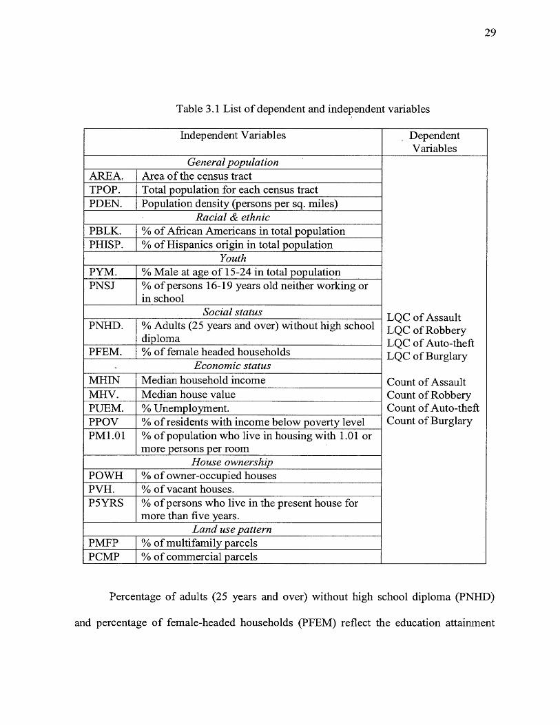
Table 3.1 List of dependent and independent variables

Independent Variables DependentVariables

General population

LQC of Assault LQC of Robbery LQC of Auto-theft LQC of Burglary

Count of Assault Count of Robbery Count of Auto-theft Count of Burglary

AREA. Area of the census tractTPOP. Total population for each census tractPDEN. Population density (persons per sq. miles)

Racial &. ethnicPBLK. % of African Americans in total populationPHISP. % of Hispanics origin in total population

YouthPYM. % Male at age of 15-24 in total populationPNSJ % of persons 16-19 years old neither working or

in schoolSocial status

PNHD. % Adults (25 years and over) without high school diploma

PFEM. % of female headed householdsEconomic status

MHIN Median household incomeMHV. Median house valuePUEM. % Unemployment.PPOV % of residents with income below poverty levelPM1.01 % of population who live in housing with 1.01 or

more persons per roomHouse ownership

POWH % of owner-occupied housesPVH. % of vacant houses.P5YRS % of persons who live in the present house for

more than five years.Land use pattern

PMFP % of multifamily parcelsPCMP % of commercial parcels

Percentage of adults (25 years and over) without high school diploma (PNHD)

and percentage of female-headed households (PFEM) reflect the education attainment

30

and family status of each census tract because people with low education background and

female (or single) headed household are two important indicators for crime analysis

(Roncek and Maier, 1991; Zhao and Thurman, 2001). Median house value (MHV),

median household income (MHIN), percentage of residents with income below poverty

level (PPOV), percentage of unemployed people in labor force (PUEM), and percentage

of population who live in housing with 1.01 or more persons per room (PM 1.01) are a

group of variables representing the economic status (Beasley and Antunes, 1974; Kohfeld

and Sprague, 1988). Both theoretical and empirical literature has concluded that low

economic status is highly associated with crimes. Since census tracts have relatively

homogeneous socio-economic characteristics, median household income was used to

represent the general income level of each tract (although income inequality is often used

by the literature as an indicator of the relative social deprivation) (Ackerman, 1998;

Belknap, 1989; Box, 1987; Braithwaite, 1978; Weatherbum, 2001).

Percentage of owner-occupied houses (POWH), percentage of vacant houses

(PVH), and percentage of people who live in the present houses for more than five years

(P5YRS) were dimensions used to capture the housing characteristics and the community

mobility. This has been found by prior research to be highly correlated with crime

(Ackerman, 1998; Ellis and Walsh, 2000; Rice and Smith, 2002; Tockovsky, 1983; Zhao

and Thurman, 2001). The last two variables - percentage of multifamily parcels (PMFP)

and percentage of commercial parcels (PCMP) were selected to test the effects of

commercial and multifamily land uses on the occurrence of crimes (Olligschlaeger,

31

1997). It is commonly believed by citizens that these two kinds of land uses are more

prone to attract crimes than single residential houses.

In general, based on the relevant theories and previous research, these 19

variables can be briefly divided into two categories: stress and control variables. PBLK,

PCMP are referred as stress variables, while AREA, TPOP, MHV, MHIN, POWN,

P5YRS are referred as control variables regarding the statistical analysis.

3.3 LQC as the Measure of Crime

The location quotient can be used to evaluate the degree to which a region

specializes in a certain crime at various levels o f geographical scales. This research uses

Brantingham and Brantingham’s (1995) equation for calculating the location quotients of

Where:

LQC* is the location quotient of crime i for small area n.

n = small area unit (census tract) under study

N = total number of area units (total number of census tracts across the city of Omaha)

Ci = count of crime i

Ct = total count of all crimes.

PHISP, PYM, PNHD, PFEM, PM1.01, PVH, PUEM, PDEN, PPOV, PNSJ, PMFP,

assault, robbery, auto-theft, and burglary crimes for each census tract.

LQC (Equation 1)

32

The LQC for crime i within an areal unit (n) is an index that compares the area’s

share of crime i with crime z’s share of the total crime across the larger area. If LQC is

bigger than 1, it means that the small area has a higher relative occurrence o f crime i

compared to the reference area. The advantage of LQC is that it highlights an area’s

relative specialty in crimes regardless of the area’s total number of crimes or population

size (Carcach and Muscat, 2002). However, there are two problems with using of LQC as

the measure of crime: (1) values below the reference average are compressed between 0

and 1; but above the norm it can rise to any value (Shaw and Wheeler, 1994); (2) if an

area has a very a small number of crimes, such as 1 or 2 with the same crime type for the

entire year, the LQC for this kind of crime in this area must be bigger than 1. In this case,

LQC can also give people a misleading impression of the profile of crime occurrence.

Another problem is that the sampling distribution of location quotients as a spatial index

is not clearly known (Shaw and Wheeler, 1984), although Carcach and Muscat (2002)

use LQCs as dependent variables to statistically analyze the crime distribution in

Australia. So the significance of using location quotients as the dependent variable needs

to be tested in this research.

3.4 GIS-based Crime Analysis

3.4.1 Data Geocoding

To locate the crime incidents, the geocoding process is the first step. Geocoding

is the method of matching the crime records with street addresses in the database with the

corresponding points in the digital (target) map file. It is the fundamental step for

displaying the spatial pattern of crimes and for getting data to perform further statistical

33

analysis. Crime records almost always have street addresses or other location attributes,

and this information enables the link between the database and the map. The street shape

file of Omaha was used as reference map to match the crime incident data in the A re View

program.

Understanding how ArcView matches addresses and how modifying the default

setting in Geocoding Editor can help users improve the accuracy of geocoding. The

Geocoding Editor in ArcView uses a specific set of steps to find a match for an address.

First it standardizes the addresses by dissecting the address into four components,

including street number, street name, street direction and street type. Second, it searches

the geocoding reference data to find potential candidates. Next, each potential candidate

is assigned a score based on how closely it matches the address. Finally, the address is

matched to the candidate on maps with the best score above the minimum match limit

(Minami, 2000). Users can set a different standard for geocoding preferences, such as

spelling sensitivity, minimum match score, and minimum score to be considered a

candidate according to different requirements of address matching. Besides interactive

matching, locating addresses manually can be used to increase the “hit rate”. For getting a

higher hit rate and increasing the accuracy o f matching, the three indices of geocoding

preferences were first set to 100 percent to do the Batch Match, and then they were

changed to relatively low values, so Interactive Match Tool could be used to locate the

unmatched addresses after the first round match.

There are a variety of reasons why not all addresses for crime could be geocoded.

Common field errors include: Sometimes the exact location of a crime is unknown.

34

Human errors can happen at several steps in the process. For example, the wrong street

type may have been recorded, the order of two digits in an address was reversed, the

street type is input incorrectly into the category of the street name or an extra zero was

inadvertently added during data entry. The reference street files also may contain errors

describing street segments. The computer software cannot recognize certain addresses

that actually exist in the real world, but are not present in the street database. Even when

a crime is geocoded, however, it could still be placed in the wrong position on the map.

For example, during the geocoding process, the incident of “Assault, 1114 N 26 Street”

can be easily drawn to the N 264th street (with highest matching score of 87) by the

software. Although this kind of error is rare, such errors are occasionally encountered in

large data files. In this case, interactive re-matching is very important.

3.4.2 Data aggregation

Once the addresses of offenses are successfully geocoded on the map, the point

data need to be aggregated to the census tract level. One of the most powerful analytical

functions in GIS software is the flexible spatial aggregation capability to facilitate the

measurement of place-based crime. In this research, the spatial join tool in ArcView was

used to aggregate the point pattern of crime to the census tract level. To do this, first the

attribute tables of both the census tract and the geocoded crime shape files need to be

opened and then the “join” from the table menu needs to be clicked. The last step is to

use the “summarize” function to get the total number of points within the boundary of

each tract.

3.4.3 Crime mapping and crime analysis

35

For visualizing the spatial distribution pattern of assault, robbery, auto-theft, and

burglary crimes in Omaha, three kinds of mapping methods were used to display the

crime distribution. The three map methods are pin (point) map, grid cell analysis (density

map), and choropleth map. The reason that different mapping methods were used is

because each method has its advantages and limitations and can only provide certain

perspective o f the thematic information to the map-readers. For getting the big picture of

crime variation in Omaha, it is necessary to combine several map methods. Software

packages such as ArcView, ArcGIS, and Adobe Illustrator were used to make all these

maps.

1. Point maps.

Point maps are probably the most frequently used maps for crime analysis, as they

can precisely show incident locations. After geocoding, the crime incidents of assault,

robbery, auto-theft, and burglary were mapped. The advantage of the point map is that it

can give map viewers the best information where crime events happen and the

frequencies o f the occurrence. The disadvantage is that with the large amount of

“stacked” points close to each other and even overlapping (such as the auto-theft and the

burglary crimes in this research), it is almost impossible to identify the individual spots,

although people can figure out the general pattern of crime distribution (Harries, 1999;

Lu, 2000).

2. Grid cell analysis and density maps.

Grid cell analysis is an effective method for displaying the dense concentration of

crime incidents and revealing the location of hot spots of crimes. A grid cell is

36

superimposed over the point map of crime incidents, and points within cells, or within the

designated radius from the centers of the cells, are assigned to the cells. The points are

transformed into a smooth surface with data generalized to cells, and different, shadings

can be used to show the density change of crimes (Harries, 1999). Density is calculated

for each cell by summing the points found in the Search Radius and dividing by the area

of the circle in area units. The output density values will be the occurrences of the

measured number of points per specified area. The grid cell method combines the

advantages of both point maps and choropleph maps and can be efficiently used to

identify the hot spots of urban crime (Harries, 1999; Lu, 2000; Ratcliffe and McCullagh,

1998).

The spatial Analyst Extension in ArcView 3.3 was used to get the density maps of

the four types of crimes. The Search Extent was set to the Omaha tract file, and the grid

cell size and the search radius were set at 100 meters and 1500 feet (about 0.2841 mile).

Thus a grid of 178X268 (rows and columns) was wrapped onto a map of the study area.

The ArcView “Kernel” density method was used to interpolate the study area and draw the

density map.

3. Choropleth maps.

After aggregating crime point data into areas, choropleth maps were used to '

display the spatial variations of crime across census tracts in Omaha. Compared to pin

maps, choropleth map lose the positional accuracy and some of the characteristics of

geographical features may be dampened and suppressed during the process of data

transformation (Lu, 2000). In addition, because of the need of data simplification and

37

generalization, using a different classification method for map presentation may convey

different information of spatial variation of crime to map-reader (Harries, 1999 and Lu,

2000). As the “rule of thumb,” the natural breaks classification method was used to

classify the crime data.

For comparing the difference of using LQC and the count of crime for crime

mapping, both kinds of measurements were used to create choropleth maps to examine

the spatial variation of crimes across census tracts in Omaha.

Choropleth mapping method was also used to display the distribution pattern of

the selected socio-economic variables for visually checking their association with the

four types of crimes.

3.5 Statistical Analysis

The database organization and data evaluation were completed before any of the

statistical procedures were implemented. Crime data were extracted from the GIS-based

dbf file corresponding to the geocoded crime shape file. Demographic data downloaded

from the 1997 American Community Survey needed to be processed to get the specific

variables for this research. The two land use variables — percentage of multi-family

parcels (PMFP) and the percentage of commercial parcels (PCMP) were summarized

from the database of the Omaha parcel file. For conducting the final statistical analysis,

these three kinds of data were combined using SPSS statistical package.

3.5.1 Descriptive statistics

Before the regression analysis, it is necessary to check the descriptive statistics of

the dependent variables, i.e., the location quotients and count of the four types of crimes.

38

Descriptive statistics include the mean, variance, range, standard deviation, skewness,

and kurtosis. Dispersion statistics such as the standard deviation, variance, and range are

designed to measure the spread or variation of the data set. Kurtosis and skewness are

statistics that characterize the shape and symmetry of the data distribution. Meanwhile,

the multicollinearity underlying the independent variables also needs to be checked, and

Pearson correlations were used to create the correlation matrix of the predictor variables.

3.5.2 Factor analysis

Factor analysis is designed to simplify the correlation matrix and reveal the small

number of factors that can explain the correlations. It is an important method of data

independence analysis and has been employed effectively by previous literature to

delineate underlying structures in data sets (Tachovsky, 1983; Ackerman 1976, 1997;

Krivo and Peterson, 1996). There are three main stages for performing factor analysis: (1)

the construction of a correlation matrix; (2) transformation of the correlation matrix into

the component matrix; and (3) obtaining the matrix of component scores (Cadwallader,

1996).

All of the variables were entered in the factor analysis and rotated with the

orthogonal Varimax rotation method. The aim of rotation is to un-correlate all of

estimated factor score coefficients to ameliorate the potential effect of multicollinearity.

Finally, the score values of the factors are added into data set as independent variables for

regression analysis.

3.5.3 Multiple regression analysis

39

Multiple regression analysis is designed to predict and explain the variation of

dependent variables (variable Y), from a number of independent or explanatory variables

(variable X) (Shaw and Wheeler, 1985), The formula for performing multiple regression

analysis:

Y = a + b] Xj + b2X2 + ... BXi + e (Equation2)

Where, a= the intercept value

b\ to bi = partial regression coefficients

e = error term

The aim of multiple regression models is to explain the corresponding variation of

the dependent variable following the variations of the independent variables (Hair et al.

1987). In this research, multiple regression models were utilized to explore whether the

spatial variation of crime could be statistically explained by the socio-economic factors.

Specifically, the backward regression method in SPSS was selected to conduct the

regression analysis. One advantage of the backward regression method is that it enters

all the variables first and then removes them once at a time (Folster, 2001). This allows

users to select different models depending on the different removal criterion. Since the

modest number of observations (102) in this research, the Stepping Method Criteria was

set at Entry: 0.01 and Removal at 0.05 to make sure the important variables can be

included in the models. Statistics such as Variance Inflation Factor (VIF) were included

in the regression analysis to test the multicollinearity underlying the independent

variables.

40

For comparing the difference of the predictability of demographic variables to the

location quotient change of crime in each tract, the count of the four types of crimes was

also employed as dependent variables in the regression analysis, In total, four regression

models were carried out for exploring the relationship between crimes and the associated

socio-economic attributes. Model 1, Model2, and Model 3 use the location quotients of

assault, robbery, auto-theft, and burglary as the dependent variables respectively, and

Model 4 uses the count of each of the four crimes as the dependent variables. Model 1

input all the original variables into the regression process, while Model 2 just leaves

indicators that are significantly correlated with the dependent variables with VIF values

within the reasonable range. Model 3 uses the principal components of the original

demographic indicators as the predictor variables, and was designed as a control model to

mediate the biased results of the LQCs.

3.6 Summary of Chapter

The methodological design for crime mapping and the statistical analysis of

crimes was presented in this chapter. The data used for this research consists of the

counts and location quotients of assault, robbery, auto-theft and burglary, and the 19

socio-economic variables for the statistical analysis o f crimes. Three types of mapping

methods were described to display the distribution pattern of crimes. Pin maps show the

detailed location of the crime incidents, density maps display the concentration of crime

“hot spots”, and choropleth maps portray the spatial variation of crime across census

tracts. Factor analysis was designed to extract the principle components of demographic

variables and the factor scores were used as the independent variables for the regression

41

analysis. The backward regression method was used to examine the co-variance between

the dependent and the independent variables. Two types of dependent variables (count

and LQCs) and two kinds of explanatory variables (original variables and principal

components) were used to produce four models and the statistical results of different

models were supposed to be compared.

42

Chapter Four

RESULTS AND ANALYSIS

4.1 Introduction

This chapter provides the major results of this research, which include two major

parts: the crime mapping and the statistical analysis. In the GIS part, the analysis of the

distribution of crime incidents, the location of hot spots, and the areal differentiation of

the four types of crimes were presented. For the statistical analysis, the explanation and

justification of each of the statistics were specified and used to test the hypotheses of this

research. Finally, the major findings from this research were compared with the previous

research.

4.2 Visualization of Crime with GIS

GIS provides a fundamental technique for this research in two aspects: (!) it

permits the geocoding and aggregation of the crime data; and (2) it permits the crime

mapping through different kinds of mapping methods. Following is the major outcome of

crime mapping and crime analysis with GIS.

4.2.1 Point maps

In terms of address matching, getting a high “hit rate” is fundamental for

receiving an accurate map and for the statistical analysis based on the geocoded database.

Table 4.1 shows the geocoding results of the four types of crimes. Good Match means a

match score between 75 and 100 and Partial Match means a score less than 75 but above

the minimum match score. Actually, most of the crime incidents received a Perfect

43

Match (with a score of 100) (86 percent for assault, 87 percent for robbery, 86 percent for

auto-theft, and 89 percent for burglary). After manual encoding, about 93 percent of the

assault, 95 percent of the robbery, 95 percent of the auto-theft, and 96 percent of the

burglary crimes were successfully address-matched.

Table 4.1: Geocoding results of assault, robbery, auto-theft and burglary crimes

N . Match N .R ate

Crimes

Batch Match* Interactive Match FinjMatch

alRate

GoodMatch

Nomatch

Goodmatch

PartialMatch

ManuallyLocated

TotalMatch

NoMatch

Assault 86% 14% 91% 1% 1% 93% 7%(507) (84) (540) (6) (6) (552) (39)

Robbery 87% 13% 92.5% 1% 1.5% 95% 5%(748) (107) (792) (5) (13) (810) (43)

Auto-theft 86% 14% 94% 0% 1% 95% 5%(3375) (548) (3701) (6) (26) (3733) (189)

Burglary 89% 11% 96% 0% 0% 96% 4%(2905) (362) (3142) (2) ....... (1)......... (3145) (121)

*: Geocoding preferences fo r the spelling sensitivity, minimum match score, and minimum score to be considered a candidate were all set to 100% fo r getting accurate batch match results.

Figure 4.1, 4.2, 4.3, and 4.4 are point maps from address matching that depict the

distribution of those four types of crimes for the year of 2000 in Omaha. These maps

show the general pattern of the selected four types of crimes. Both violent crimes (assault

and robbery) and property crimes (auto-theft and burglary) are highly concentrated in the

eastern part of Omaha, especially in the North Omaha and the downtown area, although

there are also some small clusters of hot spots spreading across the western part of the

city. Since too many points are overlapped with each other in the eastern part of Omaha

44

and other clusters, especially for the auto-theft and burglary maps, you cannot clearly

identify the location of all crimes.

Compared with auto-theft and burglary (property crimes), both assault and

robbery (violent crimes) are more concentrated in the eastern part of the city. Although

property crimes (auto-theft and burglary) are also disproportionately distributed in the

north and downtown area, they are spread throughout the whole city.

These findings are consistent with the crime survey results conducted by the

Omaha World-Herald in 1998. In terms o f the spatial patterns, from the robbery and

auto-theft maps, one can find a linear pattern of crimes along the 90th, the 72nd, Dodge, L

Street, and the downtown areas where a lot o f business stores, apartment complexes, and

unguarded parking lots are located. These areas are frequently the location of robbery and

auto-theft crimes. By overlaying the crime incidents with the commercial and multifamily

parcel maps, a clear pattern can be found that almost all of the robbery crimes occurred

within or near multifamily and commercial land parcels (Figure 4.5). a similar positive

correlation can also be observed when overlaying the commercial and multifamily

parcels with the assaults and auto-theft crimes (Figure 4.6 and Figure 4.7).

45

oooCM

■>03

s z03E

O

c■

</>

c0>

“U■ mmmOc

303<A(A<

m As

-O 3 £cAt

ez</> s >*O ) tf* <=■ * —

a> < CO b- j

o 1□

i—=reCoCo.a'a

i - !oQ_<3 <—C3£O

o</)i2a

Figu

re 4.1

As

saul

t cri

me

incid

ents

in O

mah

a, 20

00

46

-3>TS vt- <A £C X2 ©o a-U) © ,t=<ua: CO u-J n■1□

aa -E*=:co■i>Cii>o

oLJ_CO

—ro,—O

§Qc5

_ 2■?3a

Figu

re 4.2

Ro

bber

y cri

me

incid

ents

in O

mah

a, 20

00

47

Figu

re 4.3

A

uto-

thef

t cri

me

incid

ents

in O

mah

a, 20

00

48

. - c , i

Figu

re 4.4

Bu

rglar

y cri

me

incid

ents

in O

mah

a, 20

00

49

Figu

re 4.5

M

ultif

amily

&

com

mer

cial

par

cels

and

roob

erie

s

50

t/>>* - Ar o <2(/) c —

■D SS *= C§ 3 I =f 58 I i S'

_ j < £ u o

Jv r l .Kr « w -t ^ T $ . r 4

* •> fWti i

9 - e - t o

* - J f

~ 4 - L ^ . \

<1>

Figu

re 4.6

Co

mm

erci

al &

mul

tifam

ily

parc

els a

nd as

saul

ts

11

51

Figu

re 4.7

M

ultif

amily

&

com

mer

cial

par

cels

and

auto

-thef

ts

52

4.2.2 Grid cell analysis and density maps

Utilizing die Spatial Analyst Extension in ArcView, density maps of crime

incidents were produced. Figure 4.8, 4.9, 4.10, and 4.11 display the density distribution

of the four crime incidents respectively. The “hot spots” of assault, robbery, auto-theft,

and burglary are clearly drawn out on these maps. The common characteristic of the hot

spots of these four types of crimes is that they are mainly concentrated in the eastern part

of the city, especially in North Omaha. Assaults are highly concentrated in the several

clusters in North Omaha and the downtown area. The downtown area also suffers high

occurrence of robbery, auto-theft, and burglary crimes.

To explain the distribution pattern of these hot spots, both the social

disorganization and routine activity theory are needed. The social disorganization theory

can be used to explain the high concentration of crimes in North Omaha. North Omaha

has serious social stress characteristics, such as African Americans, female-headed

households, unemployment, poverty and vacant houses, identified as indicators of crime

occurrence (referred to Appendix ID-5, 9, 13,14 and 16).

The routine activity theory can provide better an explanation of the distribution o f hot

spots in downtown Omaha and hot spots scattered in west other parts of the city. These

areas concentrate many business stores, unguarded parking lots, mobile population, mid

apartment complexes, which provide offenders more attractive targets and opportunities

to commit crimes (referred to figure 4.5, 4.6, and 4.7). Routine activity theory is also

used for explaining the hot spots of auto-theft, burglary crimes in the west Omaha.

Affluent districts tend to attract properly crimes more intensely than the disadvantaged

53

areas from the perspective of profitable targets for committing property crime (referred to

Figure 4.7, Appendix III-l 1, and 111-12) (Cascach and Muscat, 2000).

25.33-50.6450.65-75.5575.56-101.27 101.28-126.59 126.50-151.91 151.92-177.23 177.24-202.35202.56-227.66

Assault Density in Omaha, 2000X4-

l____ | City limitsI I C en su s Tract

A ssault Incidents 0 - 25.32

Dviict S o u rc e : O m a h a F \> fce D e p a r tm e n t

Figure 4.8 Density map ot assault crime in Omaha. 2000

Robbery

inRobbery Density

Data Source- Omaha Pogco Department

Omaha, 2000X

Hh|____ | City Limitsr 1 C ensus Tract

Incidents 0-20.96 20.97-41.92 41.93-02.99 62.S9-8S.9J 03.S4-104.70 104.90-125.75 125.75-146.71 146.72-167,67 167 68-1 S8.63

Figure 4.9 Density map o f robbery crime in Omaha, 2000

54

Auto-theft Density in Omaha, 2000N

+

D ata S o u rce : O m a h a F o ic e D e p a rtm en t

I I City LimitsI | C en su s Tract

Autotheft Incidents 0-31.79 51.60-103.39

[ 1 1D3.e0-155.33I 155.39-207.17

■ 207.18-253.97 I 258.98-i10.76

I 1 310.77-362.55 I 362.56-414.35 | 414J36-466.14

Figure 4.10 Density map of auto-theft crime in Omaha, 2000

Burglary Density in Omaha, 2000N

4 ~I I City LimitsI I C en su s Tract

Burglary Incidents 0-42.03 42.04-34.05 84.06-126.06 126-39-168.10 168.11-210.13 21014-252.16 252.T?-2&4.18 294.19-336.21 336.22-378.21

Data Source: Omaha P&lk̂ Cv-pai irnvrn

Figure 4.11 Density map of burglary crime in Omaha, 2000

55

4.2.3 Choropleth maps

1. LQC maps

The LQCs were used as alternative measure to map the spatial variation of crimes.

Figure 4.12, 4.13, 4.14, and 4.15 are choropleth maps showing the variances of LQC for

each of the four crimes across census tracts in Omaha. Figure 4.12 shows the LQC map

of assault crime. North Omaha and the downtown area have high values of LQC. In

addition, several tracts in south Omaha and west Omaha display relative high LQC values

as well. This means these areas have a relatively higher frequency of assault crimes in the

comparison to the city average. A similar pattern appears in Figure 4.13 that maps the

LQC of robbery. In general, the LQC maps of assault and robbery also show that the

North Omaha and downtown area have higher concentration of violent crimes.

The situations for auto-theft and burglary are distinctively different from that of

violent crime. North Omaha and the downtown area show relatively low LQC values,

while west Omaha and other areas have relatively high LQC values. This means west

Omaha has a relatively high ratio of property crime in comparison to all crimes over the

city as a whole.

For a complete picture of the specialization and structure of crimes for each

census tract, all census tracts were labeled into nine different LQC categories: auto-theft

(A); burglary (B); auto-theft and burglary (A/B); robbery and auto-theft (R/A); robbery

and burglary (R/B); robbery, auto-theft, and burglary (R/A/B); assault (S); assault and

auto-theft (S/A); assault, auto-theft and burglary (S/A/B); assault and burglary (S/B);

assault and robbery (S/R); assault, robbery and auto-theft (S/R/A); and assault, robbery

56

and burglary (S/R/B) according to their dominant crime structure (with the criterion of

LQC > 1.00) (Figure 4.16). From this structure map of dominant crimes, there are other

interesting characteristics of the distribution o f crime. Census tracts in North Omaha and

downtown areas (high-crime districts) exhibit diversified structure of dominant crimes

(such as S/R/A, S/R/B or S/A/B), but tracts in west Omaha (low-crime areas) generally

have very specialized crime structure (such as A or B or A/B). This information would

not only support police in identifying where resources should be deployed in response to

a particular type of crime but also help citizens determine what the dominant crimes are

in their neighborhood (Canter, 1995).

While LQCs can be successfully used to display the specialization and structure

of crimes for each area, caution needs to be paid when interpreting areas with

extraordinary low or high crimes. Table 4.2 lists three census tracts to illustrate the

misleading nature of LQCs. Located in the western part of the city, tract 7405

experienced only 8 crimes in the year of 2000, with only one assault and one robbery

(very rare frequencies o f crime occurrence). However, the LQCs o f these two types of

crimes are 1.87 and 1.27, which are higher than the city average. Tract 0060 is in North

Omaha and belongs to the high-crime area with 208 total crimes in 2000. Although auto­

theft and burglary have higher occurrences than the other violent crimes within the tract,

the LQCs for auto-theft and burglary are less than 1.00 and LQCs for assault and robbery

are higher than 1.00. Tract 6801 has a more ordinary level of crime occurrences in which

the higher counts of crime (auto-theft and burglary) lead to higher corresponding LQC

values.

57

Bear in mind that LQC is calculated by dividing the percentage of a particular

crime in the census tract with the percentage of this crime in the city as a whole. LQC is

sensitive to both the occurrence of other crimes in the same tract and the total frequencies

of the particular crime in the whole city. Therefore, special caution needs to be exercised

when interpreting the geographical meanings of LQCs.

Table 4.2 Count and LQCs of three example tracts

TractFips*

Count of Crime** LQCs** CommentS R A B Sum S R A B

7405 1 1 3 3 8 1.87 1.27 .83 .98 West Omaha, low-crime area

0060 30 26 90 62 208 2.15 1.27 .96 .78 East Omaha, high-crime area

6801 3 5 41 32 81 .55 .63 1.12 1.03 Medium-crimearea

* Tract Fips are referred to Appendix II** S-Assault; R: Robbery; A: auto-theft; and B: burglary

LQC emphasizes the relative specialization of the specific type of crime in the

particular census tract. It should not be confused with conventional measurements that

mainly reflect the absolute number of crimes. For the tracts above, although the count of

assault and robbery is very small in tract 7405, the total count of crimes in it is also small,

and this makes these two types of violent crimes have higher concentrations relative to

the whole city (high LQCs). Tract 0060 is the opposite of tract 7405, although auto-theft

and burglary have a higher percentage than assault and robbery within the tract, the city

has an even higher percentage of these two property crimes.

58

LC3C AssaultH 0.00 - 0.35

0.36 - 0.79

0 .8 0 -1 .2 8

Data Source: Oma ha Police Deportment

LQC of Assault Crime in Omaha, 2000

Figure 4.12 Location quotient of assault crime in Omaha. 2000

LQC Robbery| H 0.00 - 0.33

0.34 - 0.70

0.71 -1 .07

1 .0 0 -1 .62

1.63-2.21

Data Source: Omaha Police Deportment

LQC of Robbery Crime in Omaha, 2000

Figure 4.13 Location quotient o f robbery crime in Omaha, 2000

59

f OC A uto, 0.57 - 0.76

0.77 ■ 0.90

0.91 -1 .07

1.08 - 1.20

1.21 -1 .54

Data Source: Omaha Police Department

LQC of Auto-theft Crime in Omaha, 2000

Figure 4.14 Location quotient of auto-theft crime in Omaha, 2000

LC3C B urg lary0 .50-0 .71

0.72 - 0.91

0.02 -1.10 1 1.11 - 1.31

1 .3 2 -1 .8 7

LQC of Burglary Crime in Omaha, 2000

Data Source: Omaha Police Department

Figure 4.15 Location quotient o f burglary crime in Omaha. 2000

60

Crimes

K 'B

S 'A

S*A.B

:S R/B

Dominant Crimes for Each Census Tract(with LQC > 1.00 foi each ctlme)

DaM SotircP' Omaha City Police Peinrtment

Figure 4.16 Map of the crime structure for each tract, 2000

2. Count maps

Because of the reasons explained above, the spatial patterns of crimes shown in

LQC maps may be different from the maps using conventional measurement of crime

(such as frequencies of crime). It was decided, therefore, that ordinary crime count maps

also needed to be produced for this research (Figure 4.17, 4.18, 4.19, and 4.20). These

count maps show a similar spatial pattern of the crimes as compared to the point and

density maps. Assault and robbery crime are disproportionately concentrated in east

Omaha, while auto-theft and burglary crimes arc broadly spread across the city. North

Omaha and the downtown area show the highest rates of both violent and property

crimes. It is also noteworthy that some individual census tracts in other parts of the city

show high crime levels for robbery, auto-theft, and burglary crimes than the surrounding

61

areas, such as the census tracts located at the large business area near the intersection of

72 and Dodge, the large apartment complex along north 72nd street, and the industrial

corridor along the L street.

Compared with the LQC maps, the count maps show similar features in terms of

assault and robbeiy crimes. But, for the auto-theft and burglar} crimes, the count amps

and LQC maps are distinctively different. In LQC maps, west Omaha has high values

while east Omaha has low values for the property crimes. One exception is in southeast

Omaha, wheix; both LQC and count maps show a high occurrence of auto-theft crime.

By comparing the two groups of maps (LQC maps and count maps), one can get a

comprehensive profile of crime in the City o f Omaha, including both the specialization

and the seriousness of crime occurrence.

Assaults0 - 3

4 - 8

| I 9* 121 3 - 1 7

1 8 - 3 0

Assault Crime in Omaha, 2000

Data Source: Om aha Police Deportment

Figure 4.17 Count o f assault crime in Omaha. 2000

62

Robberies| 0 • 3

4 - 8

I 19-151 5 -2 4

■ 25 - 33

Robbery Crime in Omaha, 2000

Data Source: Omaha Police Deportment

Figure 4.18 Count of robbery crime in Omaha. 2000

Auto-thefts| 2 - 1 2 0 1 3 - 2 5

~ 2 6 -4 2

4 3 -6 2

■ 63 - 93

Auto-theft Crime in Omaha, 2000

Data Source: Omaha Police Deportment

Figure 4.19 Count o f auto-the ft crime in Omaha. 2000

63

Burglaries2 -1 4

~ ~ H 1 5 -2 5

2 S -3 6

3 7 - 58

50 - -31

Burglary Crime in Omaha, 2000

Data Source: Omaha Police pspBrtmarrt

Figure 4.20 Count of burglary crime in Omaha. 2000

43 Statistical Results

4.3.1 Descriptive statistics

Table 4.3 shows the descriptive statistics such as Range, Minimum. Maximum,

Mean, and Std. Deviation, Skewness, and Kurtosis of both the LQCs and the raw count of

assault, robbery, auto-theft, and burglary' (written in abbreviation as Count S, Count R,

Count A, and Count B respectively). Comparing the range of LQCs of the four crimes,

one can find that LQC S and LQC R have higher values (2.89 and 2.21) than the other

two types of property crimes (0.96 for LQC A and 1.37 for LQC B). This reflects the

difference of the distribution pattern between violent and property crimes from another

64

perspective. Violent crimes are more highly concentrated in a small proportion of the

urban area while property crimes are more scattered throughout the city.

Skewness measures the asymmetry of the data distribution. A rough guide is that

if the skewness value is more than twice of its Standard Error, it indicates a departure

from a symmetrical distribution. Table 4.3 shows that all the distributions of LQCs and

the count value of the four crimes display positive skewness. The skewness statistics of

LQC_S, LQC_B, and the count of all the four types of crimes is more than twice of their

Standard Error; this means there is a departure from symmetry for their distributions,

especially for LQC S, CountS and Count R.

Kurtosis is a measure of the extent of the observations' cluster around a central

point. Positive value means the observations cluster more and have thin tails, and vice

versa. LQC S, LQC B, Count S, Counter R, and Count B have positive Kurtosis

value, while LQC R, LQC A, and Count A have negative Kurtosis value.

Although some of the crime indicators exhibit some positive skewness and

evidence of more or less cluster than the normal distribution, ordinary least squares

(OLS) regression does not assume univariate normality, so, multiple regression models

still can be used to conduct the statistical analysis.

65

Table 4.3 Descriptive statistics of the dependent variables

Statistics Range Mini. Maxi. Mean Std.Deviation

Skewness KurtosisStatistic Std.

ErrorStatistic Std.

ErrorLQCS 2.89 .00 2.89 .8467 .6279 1.057 .239 1.285 .474LQCR 2.21 .00 2.21 .8885 .5782 .245 .239 -.843 .474LQCA .96 .57 1.54 .9923 .2162 .405 .239 -.369 .474LQCB 1.37 .50 1.87 1.0648 .2662 .543 .239 .748 .474Count S 30.00 .00 30.00 5.3922 5.9071 1.923 .239 4.158 .474Count R 33.00 .00 33.00 7.9216 7.2558 1.193 .239 .969 .474Count A 91.00 2.00 93.00 36.4804 22.5484 .601 .239 -.155 .474Count_B 89.00 2.00 91.00 30.7647 16.7280 .599 .239 .697 .474

• S-Assault, R: Robbery; A: auto-theft; and B: burglary

Table 4.4 shows the correlation matrix underlying the independent variables. It is

noteworthy that there are high correlations among these predictor variables (indicated in

bold), such as correlations between MHIN vs. MHV (.926), PPOV vs. PUEM (.779), and

PFEM vs. PPOV (.774); and high negative correlation exists between MHIN vs. PFEM (-

.779) and MHV vs. PNHD (-704). Because high correlations among independent

variables will violate the regression assumptions and produce misleading results, specific

measures need to be taken to reduce the multicollinearity.

Table

4.4

Co

rrelat

ion

matri

x of

inde

pend

ent

varia

bles

6 6

CD-

GO-

COX—cq

-0 3Ocq

M -0 3CM

CO-

COGO

c oM -CO

1^-r^ -CD

■ ’

to-

COCOX—

o oGOCM .1

04

c o■M"CDi"

-COCDCO

COCOCD .77

9 f— f— CD CD

CO-

GOCNi

i" -.091 CO

CMCMi"

CDCMtoi" -.4

70 OOCMLO

i"

CM- -.5

17.60

7

CMcqCMCDCM .74

2.3

75 OOCM■M"

x—CDCOcqi* .75

6 CM■M"cq■x— CO

l"CDCOcqi"

toCDcqi’ -.6

13-.5

93

c d -M'COcq

COtoiqi*0 3 x—cq -.4

82 CMCOCM

i ’

CO

cq»’COCOCO

CMM-cq>■

SCM

0 3COCO

i"c o

cqi" .517

-.364

.291

.241 CM

COCM .5

49 GOtoCM

to■M"CM

GO — -.494

.926 CD

CDM; -.517

.256

-.471

* c oCOCMi*

CD

CMi*CDCMcqi"

c oCOCM -.2

21

f— x—CDCDCOr

CD

CO

o>«**-•’

0 3toi" .51

6

COl"

COCOcq

CMCOCM

c o .774 ■M"

CO0 30 3

COc oCOto -.7

04 toCO

toCOcqi* -.3

70.6

29 CO1*

CD

cq .285 COto

CD .737 ■M"

.132

to -COCO

CDCMCM

COCDCOi"

GO GO x—

CD

COi"

COCM

i*CM

CM -.307 to

CO x—

COCOCDi*

CMCOCM .2

54.4

39 OOOOX—

otoCD .5

56 CMCMCD -.2

98 COCD

-.293

-.258 Ocq -.307

.010

-.004 x—

.179 D -

COCM

CO

CO -

COCOCM

COCMCM .4

99 .722 CM

D -M ;i*

c oCM

CM■M"M ;i"

toCOCMi"

COCM

-.195

.729 COtocq CO

CD .730

-.040 CDto

CDi"

CM -CMOCO

i"

c o ■M" C sl

■"

CD x—

i"CO CD to

■" -.484 COto

CO

c oCOCO

l"

COCDCO

GO■M"cq -.4

73

LZV

COCOcq

■

c o

-.046 5to

■

toCOCMi"

CD

Csl1

- - .587 ■M"

CMi" -.2

52 CMCDCMi* -.3

29 c oCM

i*CO

CO

M 'CMCM .40

1.4

29-.2

56 CMCOX—

5CMi" -.1

81 CMCDto

■

■M"COcq COcqi* -.1

41

AREA

(1

)TP

OP

(2)

PBLK

(3

)PH

ISP

(4)

PYM

(5)

|PN

HD

(6)

PFEM

(7

)MH

V (8

)PM

1.01

(9)

MHIN

(10)

POW

(11)

PVA

(12)

P5YR

S (1

3)PU

EM

(14)

PNSJ

(1

5)PD

EN

(16)

PPOV

(1

7)PM

FP

(18)

PCMP

(1

9)

67

4.3.2 Regression analysis

1. Regression Model-1

Table 4,5 shows the first round results (Model-1) of the Backward regression

analysis. The Adjusted R2 represents the proportion of the variability in LQCs of each

crime. Generally, for the four types of crimes, about one third of the variation of the

assault (LQ_S) and burglary (LQC B), and less than one third of the robbery (L Q C R )

and auto-theft (LQC A) can be explained by the variation of the selected demographic

variables. However, two serious problems exist in Model-1: (1) although all the 19

original variables were entered as independent variables, only a few of them show

significant t values (PBLK for the LQC S, PFEM for the LQC R, PHISP for the

LQC A, and AREA, PHISP and PFEM account for LQC_B), which means most of other

variables do not help explain the variances in crime; and (2) some of the variables have

very high VIF values which confirms the existence of multicollinearity underlying the

independent variables which may seriously violate the assumption of regression analysis.

Basically, a VIF value greater than 4.0 indicates the existence of high multicollinearity.

However, in Table 4.5, the highest VIF value for MHIN is 23.837, and for MHV is

13.159. Therefore, Model-1 was dropped for the above reasons. For getting valid

regression results, the multicollinearity needs to be removed from the regression process.

68

Table 4.5 Regression summaries of Model-1

LQC S LQC R LQC A LQC 3 VIFB Beta B Beta B Beta B Beta

(Constant) .558 -1.684 .966 1.810AREA 4.928E-02 .125 6.747E-02 .186 2.931 E-02 .216 -5.993E-02 -.359 3.762TPOP -1.330E-05 -.064 -7.842E-06 -.041 1.449E-05 .204 -1.311E-05 -.149 2.9 77PBLK 1.094E-02 .486 3.961 E-04 .019 -2.646E-05 -.003 -1.946E-03 -.204 6.514PHISP 9.925E-03 .162 1.106E-02 .196 8.202E-03 .389 -1.433E-02 -.550 3.915PYM -3.147E-02 -.124 1.846E-02 .079 -1.828E-03 -.021 3.190E-03 .030 1.676

PNHD 4.653E-03 .090 -9.793E-03 -.205 3.926E-03 .220 -2.839E-03 -.129 8.627PFEM 4.467E-03 .088 4.171 E-02 .897 1.710E-03 .099 -1.369E-02 -.639 7.505MHV 3.722E-07 .025 2.124E-06 .154 2.743E-07 .053 -9.051 E-07 -.142 13.261

PM1.01 1.771E-02 .076 -5.547E-03 -.026 -1.730E-02 -.217 1.840E-02 .187 2.470MHIN 5.571 E-06 .173 7.218E-06 .244 -2.401 E-06 -.217 -6.825E-08 -.005 23.837POWN -5.794E-03 -.205 1.191 E-03 .046 -4.463E-05 -.005 7.414E-04 .062 13.159PVA 5.256E-03 .052 -2.968E-03 -.032 -1.038E-03 -.030 1.039E-03 .024 4.471

P5YRS -2.171 E-03 -.041 2.968E-03 .061 -7.448E-04 -.041 5.323E-04 .024 5.077PUEM 4.067E-03 .042 2.116E-03 .024 -9.566E-03 -.289 1.014E-02 .248 3.946PNSJ 7.434E-04 .009 1.289E-03 .017 2.744E-03 .096 -3.698E-03 -.104 1.430PDEN 5.440E-05 .211 4.970E-05 .209 -4.912E-06 -.055 -1.623E-05 -.148 4.352PPOV -1.933E-03 -.045 -2.154E-03 -.055 -8.030E-04 -.055 1.817E-03 .100 9.375PMFP -1.156E-02 -.144 1.827E-02 .247 -5.223E-03 -.189 3.434E-03 .101 4.037PCMP -4.271 E-03 -.065 1.014E-02 .169 4.412E-03 .197 -7.033E-03 -.254 2.890

R2 .442 .420 .384 .444Adjusted R2 .313 .286 .242 .315

F-Test 3.418** 3.132** 2.665** 3.448***: Significant at 0.05 level; **: significant at 0.01 level.

2. Regression Model-2

Model summary

For improving the regression predictability of Model-1, the last round of

Backward regression results for the four types of crimes were checked and defined as

Model-2 (Table 4.6). Model-2 not only increases the Adjusted R2 for all the four types of

crimes (.313 to .368 for LQCJS; .286lo ,347 for LQC_R; .242 to .302 for LQC_A; and

69

.315 to .353 for LQC_B), more importantly, most of the variables left have significant t

values and all their VIF values are reasonable (less than 4.0). The F-Test for all the four

Table 4.6 Regression summaries for Model-2LQC_S LQC_R LQC_A LQC_B

B Beta VIF B Beta VIF B Beta VIF B Beta VIF

(Constant) .473**PBLK 1.401

E-02.622** 1.057

PHISP 1.641E-02

.267** 1.057

(Constant) -.835*PFEM 3.263

E-02.702** 2.622

MHIN 1.119E-05

.378** 2.890

PMFP 2.922E-02

.394** 1.168

(Constant) 1.077**AREA 4.127

E-02.305** 1.280

PHISP 9.247E-03

.438** 1.441

PM1.01 -1.434E-02

-.180 1.637

MHIN -3.084E-06

-.279* 1.823

PUEM -7.754E-03

-.234* 1.410

PMFP -7.213E-03

-.261** 1.287

PCMP 3.825E-03

.171 1.186

(Constant) 1.716**AREA -3.768

E-02-.225* 1.640

TPOP -2.117E-05

-.241* 1.802

PHISP -1.137E-02

-.436** 1.131

PFEM -1.111E-02

-.518** 1.409

PCMP -5.148E-03

-.186* 1.108

R2 .381 .367 .351 .385Adjusted R2 .368 .347 .302 .353

F-Test 30.428** 18.911** 7.257** 11.997***: Significant at 0.05 level; **: significant at 0.01 level.

70

types o f crimes are significant, which means there is a statistically significant linear

relationship between the LQCs and their associated socio-economic variables. The next

step is to check the coefficient of each of the explanatory variables.

Coefficient analysis

In table 4.6, B is the regression coefficient for each variable. Beta is the standard

scores of B values, and it represents the relative importance of the predictor variables

(Folster, 2001). For the assault crime, PBLK and PHISP are the only two variables that

contribute to the predictability of LQC_S in Model-2. As expected in the second

hypothesis, both variables show positive coefficients (.622 and .267). This is consistent

with the theory and previous literature.

For the robbery crime of Model-2, PFEM (.702), MHIN (.378), and PMFP (.394)

show significant positive contribution to LQC R change. It is reasonable to find positive

correlation for PFEM and PMFP with LQC_R, because the economic deprivation of

female-headed households and the high transition and low-income characteristics of

multifamily residential areas are important indicators of robbery. However, the positive

sign of MHIN to LQC R is contrary to the hypotheses and cannot be explained by

geographical and criminological theories. Actually, when the two maps of LQC_R and

MHIN are overlaid, one can find some negative relationship between them. From this

point, unquestioning dependence on the statistical result when interpreting the causation

of crimes is ill advised (Shaw and Wheeler, 1994).

For the auto-theft crime of Model-2, although the Adjusted R2 is just above 30

percent (.302), more variables had significant contributions to the change of LQC A, and

71

they are AREA (.305), PHISP (.438), PM1.01 (-.180), MHIN (-.279), PUEM (-.234),

PMFP (-.261), and PCMP (.171). PHISP contributed most to the change of LQC A, and

then AREA and PCMP had a smaller positive effect on it. PM 1.01, MHIN, PUEM and

PMFP had negative coefficients on LQC_A. It is understandable that positive correlation

exists between AREA and PCMP with LQC A. The larger the area and the higher the

percentage of commercial parcels, leads to a availability of cars for stealing. It is also

reasonable that MHIN has a negative sign because rich people usually take more security

measures to prevent auto-theft crime. By comparing the maps of PM 1.01 (Appendix III-

10), PUEM (Appendix III-13), and PMFP (Appendix HI-18) with LQC A, it is easy to

see their negative relationship. North Omaha and downtown area have high PM1.01,

PUEM, and PMFP values, but low LQC A values, on the contrary, west Omaha has low

values for the three socio-economic variables but high LQC_A values. PCMP shows an

insignificant coefficient may indicate that it was a weak measure o f available cars in each

census tract because of the data generalization.

For the burglary crime of Model-2, all the five variables in the model have

negative signs: AREA (-.225), TPOP (-.241), PHISP (-.436), PFEM (-.518), and PCMP (-

.186). this is the same as the combination of PM 1.01, PUEM, and PMFP for LQC A.

The negative signs of PFEM and PHISP can also be explained by checking their

distribution pattern on maps (referred to Appendix III-6 and III-9). The distribution of

LQC B has a negative association with the distribution pattern of PFEM and PHISP.

Another variable that can be reasonably interpreted is PCMP (Appendix III-19). It makes

sense for PCMP to have a negative coefficient on burglary because areas with high

72

percentages of commercial parcels (few residential parcels) have relative low occurrences

of burglaries. The negative signs of AREA and TPOP are not consistent with their

distribution patterns on maps (Appendix III-1 and III-2). This may indicate that these two

variables may not capture the socio-economic characteristics associated with the LQC

change of burglary crime.

In general, the results of Model-2 are satisfactory for explaining the variance of

LQCs of the four types o f crimes, particularly for the assault and robbery crimes. Except

for LQC_A (with an adjusted R of .302), about 35 percent of the variances of the other

three types of crimes can be accounted for by Model-2. Regarding the regression

coefficients of predictor variables for the explanation of the violent crimes, socio­

economic characteristics, such as PBLK, PHISP, PFEM, PMFP exhibit correct signs

(positive) as expected in the hypothesis. But, for the auto-theft and burglary crimes, they

have negative signs opposite of what is expected. This result can be attributed to the use

of LQCs as a measure of crime and it is consistent with the co-variance pattern of socio­

economic factors and the LQCs of crimes on maps. West Omaha shows higher LQCs in

terms of auto-theft and burglary on the maps. It can be interpreted that affluent areas tend

to experience “theft victimization” more intensively than the disadvantaged areas

(Carcach and Muscat, 2000; Harries and Norris, 1986). Unfortunately, Model-2 fails to

find positive contribution of control variables to the variance of LQCs of property crimes.

4.3.3. Factor analysis and regression Model-3

1. Factor analysis

73

The principal components method was used to extract the major socio-economic

factors from the original explanatory variables. Table 4.7 shows the total variance of the

19 original variables explained by the 6 factors with eigenvalues over 1.00. These 6

factors can explain over 80 percent of the total variance of the original variables.

Table 4.7 Total variance explained by principal components

Extraction Sums of Squared

Loadings

Rotation Sums of Squared

LoadingsComponent Total % o f

VarianceCumulative

%Total % o f

VarianceCumulative

%1 7.756 40.822 40.822 4.998 26.305 26.3052 2.396 12.609 53.431 2.734 14.387 40.6923 1.566 8.243 61.674 2.379 12.519 53.2114 1.484 7.810 69.485 2.313 12.175 65.3865 1.083 5.701 75.186 1.677 8.828 74.2146 1.035 5.445 80.630 1.219 6.417 80.630

Table 4.8 shows loadings for each of the original indicators of the 6 principal

components after Varimax rotation. F a c to r l has high positive loadings for PBLK,

PFEM, PUEM, and PPOV, and high negative loadings on MHV and MHIN. Factor_2 has

high loadings for PCMP, PVH (positive) and POWN and P5YRS (negative). Factor_3

has three high loadings for PHISP, PNHD, and PM 1.01. Factor_4 combines the

characteristics o f PYM, PDEN, and PMFP. Factor_5 reflects the influence of AREA and

TPOP. The last factor (Factor_6) has high loadings on PNSJ.

Based on patterns of loadings of the original variables on each factor, the 6 factors

were in substantive terms defined more comprehensively as low socioeconomic status,

74

commercial land use, Hispanic neighborhoods, apartment & population density, size

population, and unemployed dropouts respectively.

Table 4.8 Principal components from the factor analysis

Principal Components1 2 3 4 5 6

AREA -.190 -4.803E-03 -1.000E-01 -.415 .797 -4.387E-02

TPOP -.306 -.205 -.186 7.737E-02 .805 -8.621 E-02PBLK .880 -6.115E-03 -.160 -1.303E-02 -5.206E-02 .251

PHISP -.134 .146 .894 9.610E-02 -.146 -3.673E-02PYM .311 .248 -3.328E-02 .528 .111 -.329

PNHD .633 9.276E-02 .669 -6.701 E-02 -.181 .119PFEM .843 .174 4.854E-02 .112 -.294 -3.531 E-02MHV -.720 -5.053E-02 -.444 -.240 .131 .191

PM1.01 .323 .212 .691 .119 -3.032E-02 .183MHIN -.714 -.151 -.378 -.315 .190 .201POWN -.368 -.711 -.135 -.432 .186 3.390E-02

PVA .499 .543 .322 9.137E-02 -.139 .301P5YRS -.196 -.790 -.183 -.251 -.134 -.111PUEM .794 .123 4.126E-02 -2.239E-02 -4.590E-02 .323PNSJ .256 -2.673E-02 7.879E-02 .108 -6.986E-02 .764PDEN 3.156E-02 -5.898E-02 .107 .896 -.143 .163

PPOV .784 .373 .215 7.958E-02 -.171 .216PMFP -1.966E-02 .438 .112 .757 -.129 8.928E-02PCMP 1.202E-04 .852 8.528E-02 -7.119E-02 -.201 -.197

Defined Low socioeconomic Commercial land Hispanic Apartment & Size UnemployedFactors status use neighborhoods population density population Dropouts

2. Regression Model-3

The principal components from the factor analysis were saved as new

independent variables for conducting the regression analysis (Model-3). The results of

Model-3 are in Table 4.9. After factor analysis, the VIF values of all the predictor

variables (principal components) were reduced to 1.00, and this means that the factor

analysis completely eliminated the multicollinearity among the original independent

variables.

75

For assaults, Model-3 in Table 4.9 shows that the low socio-economic status

(F a c to rl) and the unemployed dropouts (Factor_6) are the two factors that have

significant coefficients predicting LQC_S. This result complements the explanation of

LQC S in Model-2 by adding unemployed dropouts into the combination of predictor

variables.

For robbery, low socio-economic status (Factor l), commercial land use

(Factor_2), and apartment & population density (Factor_4) account for most of the

variance of LQC R. Once again, by integrating Factor_2 (commercial land use) into the

combination of predictor variables, Model-3 provides a better explanation for clarifying

the citizen’s common view that commercial areas and apartment complexes attract more

crimes, especially robberies (referred to Figure 4.5).

For the auto-theft, Hispanic neighborhoods (Factor_3) and size population

(Factor_5) have positive coefficients for the LQC A while apartment and population

density (Factor_4) and unemployed dropouts (Factor_6) have negative coefficients. The

signs of coefficients for Hispanic neighborhoods and apartment and population density

match the direction of the two original variables: PHISP and PMFP for LQC A in

Model-2. The same explanation as for LQC A in Model-2 can be used to account for the

negative coefficients o f Factor_4 and Factor_6.

For burglary, low socio-economic status (Factor_l), commercial land use

(Factor_2), and Hispanic neighborhoods (Factor_3) all have negative signs for LQCB.

For the interpretation of the negative coefficient signs of the associated factors to LQC B

it is useful to examine their distribution maps (Appendix III-5, III-9, III-13, III-14, III-19,

76

and III-6). Same explanations for LQC A and LQC B in Model-2 can be used to

interpret the regression results.

Although the Adjusted R2s for all the LQCs of the four types of crimes in Model-3

are lower than the corresponding values in Model-2, Model-3 has advantages in

determining a better combination of predictor variables in clarifying the LQC change of

crimes, especially for the assault, robbery, and burglary. Furthermore, using

comprehensive principal components (defined factors) may be more reasonable to

explain the variance of crimes than using the original demographic variables.

Table 4.9 Regression summaries of Model-3

Factors LQC_S LQC_R LQC_A LQC_B VIFB Beta B Beta B Beta B Beta 1.000

Constant .847** .889** .992** 1.064** 1.000Low social status

(Factor_1).312 .497** .153 .263** -3.176

E-02-.147 -5.588

E-02-.210* 1.000

Commercial land use (Factor_2)

4.934E-02

.079 .154 .265** 1.704E-02

.079 -6.847E-02

-.257** 1.000

Hispanic neighborhood (Factor_3)

9.846E-02

.157 -4.976E-02

-.086 6.945E-02

.321** -8.721E-02

-.327** 1.000

Apartment & density (Factor_4)

1.535E-02

.024 .173 .298** -4.454E-02

-.206* 5.268E-03

.020 1.000

Total population (Factor_5)

-3.549E-02

-.056 -8.597E-02

-.149 4.291E-02

.199* -2.214E-02

-.083 1.000

Unemployed dropouts (Factor 6)

.174 .276** 6.849E-04

.001 -4.038E-02

-.187* 1.730E-02

.065 1.000

R2 .358 .259 .248 .228Adjusted R2 .317 .212 .201 .180

F-Test 8.819 5.532 5.224 4.686*: Significant at 0.05 level; **: signiileant at 0.01 !evel.

77

4.3.4 Control model

Because most of the previous research in the field of the analysis of crime patterns

uses raw count or crime rate as the dependent variable, Model-4 (Table 4.10) was

designed as a control model to compare the predictability of LQC as an alternative

measure of crimes. In Model-4, the dependent variables are the counts of assaults

(Count_S), counts of robbery (Count_R), counts of auto-thefts (Count_A), and counts of

burglaries (Count_B) respectively. The backward regression method was also used to

conduct the regression analysis. The regression results are shown in Table 4.10.

Generally, Model-4 has higher Adjusted R2 (.430 for Count_S, .412 for CountR, .310

for Count_A, and .314 for Count_B) than Model-2. The explanation of the specific

coefficients of the predictor variables for each type of crimes is as follows:

For the Count S, stress variables such as PBLK (.450), PM1.01 (.324), and PDEN

(.155) have positive coefficients for the occurrence of assaults. This is similar to the

regression result in Model-2 in which PBLK and PHISP are significantly associated with

LQC_S. The positive effect of PDEN is consistent with social disorganization theory

because large population and overcrowding lead to high occurrence of assault crime.

For the Count R, PFEM (.526), PM 1.01 (.244), and PMFP (.321) have positive

effects on the occurrences of robbery. PFEM and PMFP also appear as explanatory

variables in Model-2 with positive coefficients for the change of LQC R. However, the

negative sign of PNHD for robbery is puzzling.

78

Table 4.10 Regression summaries of Mode-4Count_S Count_R Count_A Count_B

B Beta VIF B Beta VIF B Beta VIF B Beta VIF

(Constant) .195

PBLK 9.525E-02

.450** 1.09

PM1.01 .706 .324** 1.147

PDEN 3.753E-04

.155* 1.057

(Constant) -3.928*

PNHD -.159 -.266* 2.308

PFEM .307 .526** 1.552

PM1.01 .654 .244* 1.848

PMFP .298 .321** 1.094

(Constant) 63.104**

AREA 3.945 .279** 1.336

PBLK .230 .284* 2.943

PHISP .487 .221* 1.519

MHV -1.41E-04

-.262* 1.885

POWN -.401 -.395** 1.528

PUEM -.944 -.273* 2.387

(Constant) 63.713**

AREA 1.905 .182 1.286

MHV -1.23E-04

-.308**

1.381

POWN -.407 -.542**

2.227

PCMP -.470 -.271* 1.592

R2 .447 .435 .351 .341

AdjustedR2

.430 .412 .310 .314

F-Test 26.417** 18.694** 8.558** 12.535**

*: Significant at 0.05 level; **: significant at 0.01 level.

For the Count_A, 6 variables appear to account for the variance of auto-thefi.

AREA, PBLK, and PHISP had positive effects while MHV, POWN, and PUEM had

negative effects. These results basically reflect the distribution pattern of auto-theft in the

79

count map (Figure 4.19). The larger the AREA and the higher the percentage of African

Americans and Hispanic population, the higher the frequencies of auto-thefts. The

negative signs of MHV and POWN can be explained that security precautions and

neighborhood watch efforts reduce the occurrence of auto-thefts. The positive sign of

PBLK confirms the second hypothesis that social stress factors have positive association

with crime and is compatible with the social disorganization theory. However, it is

difficult to explain the negative contribution of PUEM in this model.

For Count_B, PHV (-.308), POWN (-.542), and PCMP (-.271) are the three

explanatory variables that have significant coefficients for the frequencies of burglary.

The same explanation as for the auto-theft crime can be used to account for the

coefficients of PHV and POWN to burglary crime. Intensive security measures and

neighborhood watch in affluent areas effectively reduced the occurrence of burglary. The

negative coefficient of PCMP can be explained by observing that a high percentage of

commercial parcels lead to low share of residential parcels and low burglary crimes.

In general, Model-4 provides a reasonable explanation for the spatial variance

patterns displayed in the count maps and is consistent with prior research. Stress

variables, such as PBLK, PHISP, PFEM, PM1.01, PDEN, and PMFP, have the expected

positive coefficients and the control variables (such as MHV and POWN) have negative

signs for the explanation of the occurrence of specific types of crimes.

4.3.5 Evaluation of models

Comparing the results of the Model-2, Model-3 (LQC models), and Model 4

(count model), some commonalities and differences can be identified:

8 0

(1) For the two types of violent crimes, the stress variables or principal

components show expected positive signs separately or in some combination in these

three models, such as PBLK and PHISP for assaults, and PFEM and PMFP for the

robberies in Model-2; low social status (Factor l) and unemployed dropouts (Factor_6)

for assault, and Factor_l, commercial land use (Factor_2), and apartment and density

Factor_4 for robberies in Model-3; PBLK, PM1.01 and PDEN for assaults, and PFEM,

PM1.01, and PMFP for robberies in Model-4.

(2) The difference between the LQC models and count models are evident for the

property crimes. The stress variables show different signs for the LQC models (Model-2

and Model-3). PM1.01, PUEM, and PMFP have negative signs for LQC A and Factor l

has negative signs for both LQC A and LQC B in Model-3, while PBLK, PHISP have

positive signs for Count A. Comparing the LQCs and count maps of the auto-theft and

burglary can clarify this difference. On LQC maps, stress variables show a negative

relationship with property crimes while on count maps they show positive relationship

with property crimes. There are two exceptions, one is PHISP which has the same sign

(positive) for both LQC_A and Count_A; the other is PCMP which makes a positive

contribution to LQC A and has the negative coefficient for both LQC B and CountB.

(3) The control variables such as MHIN shows expected negative coefficients for

LQC A in Model-2, and MHV and POWN have negative contribution for Count_A and

Count B in Model-4, but MHIN exerts incorrect (positive) contribution to the LQC_R in

Model 2.

81

Only modest proportions of the variations of both the LQCs and count of crimes

were explained by the designed models, although these match the general level of

predictability of statistical analysis of crime, following four problems may exert negative

effects on the predicting of the statistical models in this research.

(1) Crime occurrences are determined by some random elements and numerous

factors that are still poorly understood by researchers (Ellis and Walsh, 2000).

Demographic factors are not responsible for all the occurrence of crimes in the

neighborhoods, and other issues such as access to 24-hour stores, large shopping centers,

apartment complex, interstate highways, and major roads are also important stimulators

o f crime (Napolitano, 1998).

(2) The occurrences of crimes are not necessarily at the place or area where the

offenders or victims live. From this point, it is not surprising that using the demographic

data at aggregated areal level cannot completely explain the occurrence of crimes in each

area;

(3) In this research, one year’s data o f crime cannot capture fully the general

situation of the occurrence o f crimes in the City of Omaha, since the fluctuation of the

crime rate over years;

(4) Although very high matching rate was achieved during the geocoding process,

there was still 7 percent of assault, 5 percent of robbery and auto-theft, and 4 percent of

burglary incidents that were not matched. These kinds of technique limitation definitely

affect the accuracy and validity o f this analysis.

8 2

(5) Aggregating point data to the census tract level. Some of the spatial pattern of

crime may be dampened or suppressed during the aggregation of point data to the census

tract level. The same problem affects the demographic data. Using finer areal units, such

as block group or blocks may be useful for getting more satisfactory statistical results.

(6) Particularly, for the LQC models (Model-2 and Model-3), the overestimation

or underestimation of the values of LQC for areas with extraordinary low or high crime

frequencies may also hamper the predictive power of the models.

4.4 Summary of Chapter

The results of the GIS visualization and statistical analysis of this research were

summarized in this chapter. Through geocoding, more than 93 percent of the original

crime incidents were successfully geocoded on maps. In total, three types of map

methods were used to visually display the distribution of incidents, the location of hot

spots, and the areal differentiation of assault, robbery, auto-theft, and burglary crimes in

the City of Omaha. The general distribution pattern of these four types of crimes is that

they are disproportionately concentrated in the North Omaha and the downtown area.

Assault and robbery (violent crimes) dominate North Omaha and the downtown Omaha

(high-crime area), while auto-theft and burglary (property crimes) spread to the whole

area o f the city.

LQC maps and count maps show similar picture in terms of the violent crimes,

but show different profile for the two types of property crimes. On the LQC maps, auto­

theft and burglary exhibit higher values in west Omaha and low values in the eastern part,

while on the count maps they show higher value in the eastern part and low values in the

83

western Omaha. The specialization and structure map of LQCs shows that different areas

have different crime specialization and crime structure. High-crime areas such as North

Omaha and downtown area generally have a diversified structure of crimes, while low-

crime areas such as west Omaha have relatively specialized structure of crime — mostly

property crimes. LQC has advantages in displaying the relative occurrence of crime in

each census tract compared to the city average while the count of crime indicates the

absolute occurrences (the seriousness of crime) o f crime within each tract.

For the statistical analysis, four models were produced. However, Model-1 was

discarded for the serious violation of regression assumptions, only Model-2, Model-3,

and Model-4 were kept to explain and test the hypotheses. Model-2 uses LQCs as

dependent variables and shows that modest proportion (about 35 percent for the assault,

robbery and burglary crimes and about 30 percent for auto-theft crime) of the variance of

the four types of crimes can be significantly explained by the selected socio-economic

variables. The stress variables such as PBLK, PHISP, PFEM, PMFP show expected

positive contribution to the violent crime, but show unexpected negative signs for the

property crimes. This is because of LQCs were used as dependent variables. But, the

control variables such as MHV, POWN, and P5YRS are either not necessary or exert the

opposite influence as expected, such as the positive sign of MHIN for LQC R in Model-

2 .

Factor analysis not only completely eliminates the multicollinearity underlying

the independent variables but also has the advantage of creating reasonable combinations

84

of explanatory variables and results in using principal components as independent

variables in Model-3.

Model-4 was included as a control model (using count of crime as the dependent

variable) to compare with the LQC models. It had higher Adjusted R s than the

corresponding LQC models (Model-2 and Model-3). Stress variables such as PBLK,

PHISP, PFEM, PM1.01, PDEN, and PMFP separately or in some combination had

expected positive coefficients while the control variables such as MHV and POWN had

the expected negative signs for both the violent and property crimes. The results of

Model-4 match the distribution pattern of crimes on the count maps and is compatible

with the social disorganization theory and previous research.

The LQC models and count models share some commonalities and each exhibits

distinctive advantages in reflecting different aspects of the occurrence of crime across

areas. Model-2 and Model-3 can be integrated for analyzing the relative specialization

and structure of crimes across space, while Model-4 is superior in examining the absolute

frequencies of crimes.

There are several reasons that may explain the modest predictability of the

regression model. Socio-economic characteristics may not account for all the occurrence

of crimes, and there are crime factors that are still obscure for researchers. Problems

concerning the GIS-based geo coding and generalization problems with data aggregation

also reduce the predictability of the regression models. In addition, problems with using

LQCs may also hamper the explanation power of the LQC models.

85

Chapter Five

CONCLUSION

5.1 Overview of Thesis

The major purpose of this thesis is to display the spatial distribution pattern of

assault, robbery, auto-theft, and burglary crimes in the City o f Omaha and explore their

relationship with the selected socio-economic characteristics. The location quotient of

crime (LQC) was employed as an alternative measure to capture the specialization and

structure of dominant crimes across census tracts. Chapter One addressed the nature of

the problem, the objectives, hypotheses, and significance of this research. The major

theories and previous research literature on crime mapping and crime analysis were

reviewed in Chapter Two. Chapter Three presented the methodology of the thesis, and

both the approaches o f GIS visualization and statistical analysis were included in this

research. Three kinds of mapping methods (point, grid cell analysis, and choropleth map)

were used to display the location of crime incidents, the hot spots distribution, and the

spatial variation of crimes across census tracts. For the statistical analysis, both factor

analysis and multiple regression models were used to explore the crime-causation

relationship. Chapter Four presented the results and analysis of the map interpretation and

statistical models.

5.2 Major Findings of Research

Through this research, the distribution pattern of the four types of crimes and their

relationship with socio-economic characteristics were explored. The major findings of

this research include:

85

86

(1) Through the mapping of the crime incidents, the analysis of hot spots and the

areal differentiation, the major profile of crime in Omaha is that crimes are unevenly

distributed in the city and all the four types of crimes show a high concentration in the

eastern part of the city, especially North Omaha and the downtown area. Specifically,

assault and robbery exhibit a more disproportionate distribution pattern than property

crime and is mainly dominated by the North Omaha and downtown areas, while property

crime is spread throughout the whole city.

(2) The LQC has the advantage of highlighting the relative specialization of

crime across geographical areas and can be successfully used as an important alterative to

the conventional measures for crime mapping. The LQC maps of each of the four types

of crimes and the structure map of dominant crimes in each census tract show that east

Omaha has a higher occurrence of violent crime and diversified crime structure while the

western part o f the city is dominated by property crime and has relatively specialized

structure of crimes. This finding is not only helpful for supporting police to find the

dominant crimes for each area and to deploy rational resources in response to different

structure o f crimes, but also helps citizens determine out the prevailing crimes in their

neighborhoods.

However, the LQC may also cause a misleading perception of crime distribution.

Special caution needs to be exercised in the interpretation of LQCs for areas with

extraordinary low or high occurrences of crime to avoid a biased conclusion. Therefore,

integrating the conventional measure (count or crime rate) is advised when using LQCs

for crime mapping and statistical analysis.

86

87

(3) The regression model using LQC as a dependent variable can significantly

explain a modest proportion of the specialization of four types of crimes. The control

model (regression model using count o f crimes as dependent variables) produced similar

results for the assault and robbery crimes as the LQC models, but quite different results

for the auto-theft and burglary crimes. This simply reflects the difference between the

LQCs and the count of the property crimes in Omaha.

Social tress variables such as PBLK, PHISP, PFEM, PM1.01, PDEN, and PMF

had the expected signs (positive) for both LQC and count models, separately or in

combination, for the assault and robbery crimes. But, PM 1.01, PUEM, PMFP, PHISP,

PFEM, and PCMP had negative coefficients for the auto-theft and burglary crimes in

Model-2, which is contrary to the second hypothesis. This finding has an implication in

enriching the application of LQCs for conducting multiple regression analysis andr

explaining the prevailing situation of property crime in the affluent areas (west Omaha)

of the city. Control variables such as MHV and POWN had the expected negative

coefficients to the occurrence of property crime in the count model.

The two kinds of statistical models (LQC model and count model) had distinctive

advantages in accounting for the different aspects of the crime (relative specialization or

absolute occurrence of crime) and can be used to justify the general spatial patterns of

crime in the corresponding LQC maps and count maps.

(4) Factor analysis is an effective method for reducing the multicollinearity that

exists in the predictor matrix but did not necessarily improve the predictability in the

regression analysis by using the principal components as independent variables. Although

87

88

factor analysis does not lead to a higher Adjusted R2s than Model-2, Model-3 exhibits

some particular compensation in determining a better combination of predictor variables

and provides more reasonable explanation of the variance of crimes than using the

original variables. For example, low social status, commercial land use, and apartment &

density had positive coefficients on LQCRobbery. This finding clarified the citizen’s

common view that apartment and commercial areas attract more crimes.

5.3 Future Work

More research is needed to focus on various aspect o f crime analysis that could

not be addressed in this thesis. The multiple regression models used in this research,

could only explain about one third of the variation of the change in the dependent

variable. Therefore further research is needed to improve the geographical predictability

of crime. Specifically, five aspects are possible for future study in crime mapping and

crime analysis.

(1) Focus on a specific type of crime to explore its spatial pattern and causation.

The major purpose the research presented here was to examine the general profile of

crime in the City of Omaha. For future studies, choosing an individual crime to conduct

in-depth analysis is essential.

(2) Use finer spatial units, like block groups or blocks. Although census tracts can

be successfully used to study the variations of crimes, using a finer unit of observation

may greatly increase the accuracy of both the crime and demographic data and achieve a

higher level of explanation.

88

89

(3) Including more detailed variables, such as the number of bars, number of

entertainment center for youth, number of gas stations and 24-hour stores, may account

for a higher proportion of variance of crimes over time and across space.

(4) Focus on crime hot spots. Using location quotients to analyze the

concentration and extent of dominant crimes in risk areas (hot spots) or examining the

distribution pattern of crime over time would be interesting areas of research.

(5) Examine longer periods of crime data. The common practice is to use several

years (usually three years) of crime data for statistical analysis to reduce the annual

fluctuations and enlarge the possibilities of crime incidents for some low-crime areas.

Furthermore, including time-series analysis of crime along with sector analysis is also

helpful in revealing the nature of crime over time and space.

(6) The spatial autocorrelation needs to be taken into consideration. Because of

the limitation of time and software, spatial autocorrelation was not examined when

conducting the multiple regression analysis. Spatial autocorrelation has been addressed

by previous researchers in recent years when conducting regression analysis based on

small areal units (i.e., census tracts and blocks) (Brown 1982; Mencken and Barnett

1999; Messener et al. 1999; Murray et al. 2001; Rice and Smith 2002; Roncek and Maier

1991; Rosenfeld et al. 1999; Weatherbum and Lind 2001). Therefore, checking the

existence of spatial autocorrelation among observations and adding a specific variable

reflecting the spatial autocorrelation to control the neighborhood effects is essential for

the future studies. Software package such as SpaceStat can be used for the spatial

autocorrelation analysis (Vania et. al., 2002).

89

90

References

Ackerman, William V. (1998). Socioeconomic correlations of increasing crime rate in

smaller communities. Professional Geographer. 50(3), 372-387

Agnew, Robert. (1999). A general strain theory of community differences in crime rates.

Journal of Research in Crime & Delinquency. 36(2), 123-155.

Anselin, Luc; Cohen, Jacqueline; Cook, David; Gorr, Wilpen; and Tita, George. (2000)

Spatial analysis of crime. In: Measurement and Analysis of Crime and Justice.

Criminal Justice, 2000. vol. 4 U.S Department of Justice, Office of Justice

Programs. Washington, U.S.

Beasley, Ronald W. and Antune George. (1974). The etiology of urban crime: an analysis

of ecological analysis. Criminology, 11(4), 439-461.

Belknap, J., (1989). The economics-crime link. Criminal Justice Abstracts, March, 140-

157.

Bellair, Paul E. (1997). Social interaction and community crime: examining the

importance of neighbor networks. Criminology, 35: 677-703.

Box, S., (1987). Recession, Crime and Punishment. Macmillan, London, 68-229.

Brantingham, P. J. and P. L. Brantingham. (1995). Location quotients and crime hot spots

in the city. In block, C.R., Dabdoub, M. and Fregly, S.(eds). Crime Analysis

through Computer Mapping Washington, DC: Police Executive Research Forum;

Brantingham, P. J. and P. L. Brantingham. (1997). Mapping crime for analytic purpose:

location quotients, counts, and rates. Crime Mapping & Crime Prevention. Crime

Prevention Studies, vol. 8. Criminal Justice Press. Monsey, New York, U.S.A

90

91

Braithwaite, J., (1978). Unemployment and adult crime: an interpretation of the

international evidence, In: Unemployment and Crime: Proceedings of Institute of

Criminology, no. 36, Sydney University, 54-71.

Brimicombe, Allan J.; Ralphs, Martin P.; Sampson, Alice; and Hoi Yuen Tsui. (2001).

An analysis of the role of neighborhood ethnic composition in the geographical

distribution of racially motivated incidents. British Journal of Criminology. 41,

293-308

Brown, Marilyn. (1982). Modeling the spatial distribution of suburb crime. Economic

Geography. 58(3), 247-261.

Bursik, Robert J. Jr. (1988). Social disorganization and theories of crime and

delinquency: problems and prospects. Criminology 26: 519-551

Bursik, Robert J. Jr. and Webb, Jim. (1982). Community change and patterns of

delinquency. American Journal of Sociology 88:24-42.

Cadwallader, Martin (1996). Urban Geography: an analytical approach. Prentice Hall.

Canter, Philip R. (1997). Geographic information systems and crime analysis in

Baltimore County Maryland. Crime Mapping & Crime Prevention. Crime

Prevention Studies, vol. 8. Criminal Justice Press. Monsey, New York, U.S.A

Carcach, Carlos and Muscat, Glenn. (2000). An analysis of regional variations in crime

using crime concentration indexes. Conference on Crime Mapping: Adding Value

to Crime Prevention and Control. Australia Institute of Criminology 21-22

September.

Carcach, Carlos and Muscat, Glenn, (2002). Location quotients of crime and their use in

91

92

the study of area careers and regional crime structures. Crime Prevention and

community: An International Journal. 4 (1), 27-46

Chiricos, T., (1987). Rates of crime and unemployment: an analysis of aggregate research

evidence. Social Problems 34(2) 187-212

Cohen, Lawrance E.; and Marcus Felson. (1979). Social change and crime rate trends: a

routine activities approach. American Sociological Review 44: 588-608

Crime in the United States, 2000, Uniform Crime Reports. Federal Bureau of

Investigation. U.S. Department of Justice, Washington, D.C.

Ellis, Lee and Walsh, Anthony. (2000) Criminology: A Global Perspective. Allyn &

Bacon. MA 02494

Folster, Jeremy J. (2001). A Beginner’s Guide: Data Analysis- Using SPSS for Windows.

New Edition: Versions 8-10. Sage Publications.

FBI 2000 Uniform Crime Report, Washington, DC 20535.

Garrett Nagal. (1995). Urban crime: a geographical appraisal. Geographical Magazine.

67(3), 56-56

Gisela Bicheler-Robertson and Johson, Melissa. (2001). Connecting environmental cues

to commercial burglary concentrations: combining theory and practice into a

tHblended approach. Paper presented at the 10 International Seminar on

Environmental Criminology and Crime Analysis, 18 June 2001.

Harries, Keith, (1994). Juvenile gun crime and social stress: Baltimore, 1980-1990.

Urban Geography 15 (1), 45-63.

Harries, Keith, (1999). Mapping Crime: Principle and Practice. U.S. Department of

92

93

Justice, Office of Justice Programs, National Institute of Justice. Washington, DC.

Harries, Keith; and Norris, Robert E. (1986). Human Geography: Culture, International

and Economy. Merrill Publishing Company. Columbia, Ohio. 43216.

Herbert, D. J.; and Hyde, S. W. (1984). Residential crime and the urban environment

Unpublished report to the Economic and Social Reseach Council, Department of

Geography, University College of Wales, Swansea.

Hirschfield, A. and K. J. Bowers. (1997). The effect of social cohesion on levels of

a recorded crime in disadvantaged areas. Urban Studies. 34 (8), 1275-1295.

Kasarda, John D.; and Morris Janowitz. (1974). Community attachment in mass society.

American Sociological Review 39: 328-339

Kohfeld, Carol W. and Sprague, John. (1988). Urban unemployment drives urban crime.

Urban Affairs Quarterly 24(2), 215-241

Krivo, Lauren J. and Peterson, Ruth D. (1996). Extremely disadvantaged neighborhoods

and urban crime. Social Forces. 75(2), 619-648.

Linsky, Arnold S.; and Straus, Murray A. (1986). Social Stress in the United States—

Links to Regional Patterns in Crime and Illness. Auburn House Publishing

Company, Denver, Massachusetts.

Lu, Y. (2000). Spatial cluster analysis of point data: location quotients versus kernel

density. 2000 University Consortium of Geographic Information Science

(UCGIS). Summer Assembly Papers. Portland, Oregon.

(http ://www.uc gis.org/ore gon/papers/lu.htm)

Marshall, Chris E. (1990). Crime in the Omaha area: perceptions, protective, measures,

93

94

and victimization. Omaha Conditions Survey: 1990. Center for Public Affairs

Research.. University of Nebraska at Omaha.

Massimo, Craglia, et al. (2001). Modeling high-intensity crime areas in English cities.

Urban Studies. 38(11), 1921-1941.

McClain, Paula D. (1989). Urban black neighborhood environment and homicide: a

research note on a decade of change in four cities, 1970-1980. Urban Affairs

Quarterly. 24, 584-96.

Meithe, Terance D., and Robert F. Meier. (1994) Crime and Its Social Context. Albany:I

State University of New York Press.

Mencken, F. Carson and Barnett, Cynthia. (1999). Murder, nonnegligent manslaughter,

and spatial autocorrelation in Mid-South counties. Journal of Quantitative

Criminology. 15(4).

Messner, Steven F.; Anselin, Luc; Bailer, Robert, D.; Hawkins, Darnell F.; Deane, Glenn;

and Tolnay, Stewart E. (1999). The spatial patterning of county homicide rates: an

application of exploratory spatial data analysis. Journal of Quantitative

Criminology. 15(4), 423-450.

Minami, Michael. (2000). Using ArcMap: GIS by ESRI. Environmental Systems

Research Institute, Inc. CA92373-8100, USA.

Murray, Alan T., McGuffog, Ingrid, Westerm, John S., and Mullins, Patrick. (2001).

Exploratory spatial data analysis techniques for examining urban crime. British

Journal of Criminology. 41, 309-329.

Napolitano, Carol, et al. (1998). Omaha crime: a special report. Omaha World-Herald,

94

95

November 8, 1998.

Olligschlaeger, Andreas M. (1997). Spatial analysis of crime using GIS-base data:

weighted adaptive filtering and chaotic cellular forecasting with applications to

street level drug markets. Ph.D Dissertation, Carnegie Mellon University.

(http://www-2.cs.cmu.edu/~olli/dissertation.html)

Ousey, Graham C. (1999). Homicide, structural factors, and the racial invariance

assumptions. Criminology 37: 405-426.

Ousey, Graham C. (2000). Explaining regional and urban variation in crime: A review of

Research. The Nature of Crime: Continuity and Change. Criminal Justice, Vol. 1.

U.S. Department of Justice, Office of Justice Programs

Pierce, G., S. A. Spaar, and L. Briggs IV. (1988). The character of police work: strategic

and tactical implications. M. S. Thesis, Northeastern University, Center for

Applied Social Research.

Ratcliffe, J. H. and M. J. McCullagh. (1998). The perception of crime hot spots: a spatial

study in Nottingham, UK. In: N. La Vigne and J. Wartell, eds: Crime Mapping

Case Studies: Successes in the Field. Washington, DC: Police Executive Research

Forum, 45-51.

Reith, Margaret. (1996). The relationship between unemployment in society and the

popularity of crime drama on TV. Journal of Broadcasting & Electronic Media.

40(2), 258-264.

Rice, Kennon J. and Smith, William R. (2002). Socioeconomic models of automotive

95

96

theft: integrating routine activity and social disorganization approaches. Journal of

Research in Crime and Delinquency. 39 (3), 304-336.

Rosenfeld, Richard; Bray, Timothy M.; and Egley, Arlen. (1999). Facilitating violence: a

comparison gang-motivated, gang-affiliated, and nongang youth homicide.

Journal of Quantitative Criminology. 15(4), 495-517.

Roncek, Dennis and Maier, Pamela. (1991). Bars, blocks, and crimes revisited: linking

the theory of routine activities to the empiricism of hot spots. Criminology, 29 (4).

Sampson, R. and Byron Groves. (1989). Community structure and crime: testing social

disorganization theory. American Journal of Sociology. 94, 774-802

Sampson, Robert J.; Raudenbush ,Stephen W.; and Earls, Felton. (1997). Neighborhoods

and violent crime: a multilevel study of collective efficacy. Science 277: 918-924

Shaw, Clifford R. and Henry D. Mckay. (1942). Juvenile Delinquency and

Urban Areas. Chicago, The University of Chicago Press

Shaw, Gareth; and Wheeler, Dennis. (1994). Statistical Techniques in Geographical

Analysis. Second Edition. Halsted Press, New York.

Sherman, L. W.; P. R. Gartin; and M. E. Buerger (1989). Hot spots of predatory crime:

routine activities and the criminology of place. Criminology, 27: 27-55.

Sherman, L. W. (1992). Attacking crime: police and crime control. In Moden Policing.

edited by M. Jonry and N. Morris. Vol. 15 of Crime and Justice: A Review of

Research. Chicago: University of Chicago Press.

Slovak, Jeffery S. (1986). Attachments in the nested community: evidence from a case

study. Urban Affairs Quarterly 21: 575-597

96

97

Tachovsky J.C. (1983). Ecological correlates of crime for New Castle County, Delaware:

a canonical analysis. Pennsylvania Geographer. 21(3-4), 43-70.

Vania Ceccato; Robert Haining; and Paola Signoretta. (2002). Exploring offence

statistics in Stockholm City using spatial analysis tools. Annals of Association of

American Geographers. 92(1), 29-51.

Warner, Barbara; and Pamela Wilcox Rountree. (1992). Local social ties in community

and crime model: questioning the systemic nature of informal social control.

Social Problems, 44: 520-536.

Weatherbum, Don, and Lind, Bronwyn. (1997). Social & Economic Stress, Child Neglect

and Juvenile Delinquency. Bureau of Crime Statistics and Research.

http://www.agd.nsw.gov.au/bocsarl. risf/pages/s&estresssumm

Weatherbum, Don, and Lind, Bronwyn. (2001). Delinquent-Prone Communities

Cambridge University Press.

Weisburd, d. L.; and L. Green. (1994) Defining the street level drug markets. In Dmgs

and Crime: Evaluating Public Policy Initiatives, edited by D. L. Mackenize and C.

D. Uchida. Beverly Hills: Sage Publications.

Zhao, Jihong; and Thurman, Quint. (2001). A national evaluation of the effect

of cops grants on crime from 1994 to 1999. Department of Criminal Justice,

University of Nebraska at Omaha. December 2001.

97

98

Appendix 1-1: Crime Data

TractCount_S Co.(jnt_R

Count_A

Count_B

LQC-T ypes LQC_S LQC_R

ioa—

i < LQC_B

2 3 14 ’ 34 21 R/A 0.62 1.98 1.04 0.763 26 18 46 45 S/R 2.88 1.36 0.75 0.874 6 3 27 35 S/B 1.26 0.43 0.84 1.295 4 3 58 44 A/B 0.55 0.28 1.18 1.066 8 8 47 42 S/B 1.14 0,77 0.99 1.057 7 10 33 50 S/R/B 1.05 1.02 0.73 1.318 8 10 31 32 S/R/B 1.48 1.26 0.85 1.039 1 9 17 21 R/B 0.31 1.91 0.78 1.1510 11 12 24 34 S/R/B 2.03 1.51 0.65 1.111 9 17 40 52 S/R/B 1.14 1.47 0.75 1.1512 13 19 62 43 S/R 1.42 1.41 1 0.8216 6 6 60 24 A 0.93 0.64 1.38 0.6518 15 23 93 44 S/R/A 1.28 1.34 1.17 0.6619 4 7 40 34 A/B 0.7 0.84 1.04 1.0520 11 22 75 30 S/R/A 1.19 1.62 1.2 0.5721 3 5 45 18 A 0.63 0.72 1.4 0.6622 1 0 17 11 A 0.52 0 1.29 0.9923 2 0 30 17 A 0.61 0 1.35 0.9124 11 7 44 40 S/B 1.61 0.7 0.95 1.0325 3 2 34 27 A/B 0.68 0.31 1.14 1.0726 3 5 50 28 A 0.52 0.59 1.28 0.8527 11 14 46 34 S/R 1.57 1.36 0.97 0.8528 4 3 55 30 A 0.65 0.33 1.32 0.8529 20 12 80 47 S/A 1.88 0.77 1.11 0.7730 2 2 39 13 A 0.53 0.36 1.54 0.6131 6 6 76 39 A 0.71 0.48 1.32 0.832 5 4 50 14 S/A 1.02 0.56 1.51 0.533 2 6 32 25 A/B 0.46 0.94 1.09 1.013401 2 1 27 24 A/B 0.55 0.19 1.1 1.163402 2 1 12 20 B 0.85 0.29 0.76 1.535 5 9 19 40 S/R/B 1.02 1.25 0.57 1.4336 2 5 15 18 R/B 0.75 1.27 0.83 1.1837 0 2 7 11 R/B 0 . 1.02 0.77 1.4438 6 9 47 47 B 0.82 0.84 0.95 1.1339 24 27 54 49 S/R 2.33 1.78 0.77 0.8340 7 11 34 43 S/R/B 1.1 1.18 0.79 1.1941 2 13 25 28 R/B 0.44 1.94 0.81 1.0842 1 6 20 22 R/B 0.3 1.25 0.9 1.1843 7 24 44 49 R/B 0.84 1.97 0.78 1.0344 2 15 36 24 R/A 0.39 1.98 1.03 0.8245 1 4 9 10 R/B 0.62 1.69 0.83 1.0946 0 0 6 15 B 0 0 0.63 1.8747 0 0 5 12 B 0 0 0.65 1.8548 3 22 74 45 R/A 0.31 1.55 1.13 0.82

99

49 12 33 91 91 R/B 0.79 1.48 0.89 1.0550 8 21 45 58 R/B 0.91 1.62 0.75 1.1551 6 13 39 47 R/B 0.85 1.26 0.82 1.1752 21 20 44 41 S /R 2.49 1.61 0.77 0.8553 12 11 55 46 S 1.45 0.9 0.98 0.9754 14 9 42 48 S/B 1.85 0.81 0.82 1.1155 2 4 31 35 B 0.42 0.56 0.95 1.2756 1 6 48 33 A 0.17 0.69 1.2 0.9857 1 18 31 33 R/B 0.18 2.21 0.82 1.0458 10 11 57 64 S/B 1.05 0.79 0.89 1.185901 12 14 34 42 S/R/B 1.76 1.4 0.74 1.085902 11 6 50 26 S/A 1.77 0.66 1.19 0.7360 30 26 90 62 S /R 2.15 1.27 0.96 0.786101 17 6 29 36 S/B 2.89 0.69 0.73 1.076102 8 9 37 49 S/B 1.16 0.89 0.79 1.256202 10 14 61 48 S/R/A 1.12 1.07 1.01 0.956301 2 4 40 28 A 0.4 0.55 1.19 0.996302 8 5 51 32 S/A 1.25 0.53 1.17 0.876303 6 4 28 22 S/A 1.49 0.68 1.03 0.9664 3 6 28 32 B 0.65 0.88 0.9 1.216501 2 7 46 42 A/B 0.31 0.73 1.05 1.136502 1 6 31 29 A/B 0.22 0.91 1.02 1.136601 5 21 77 46 R/A 0.5 1.43 1.14 0.816602 2 9 18 18 R 0.64 1.95 0.85 16701 6 21 53 35 R/A 0.78 1.86 1.02 0.86702 2 6 37 15 R/A 0.5 1.02 1.36 0.656801 3 5 41 32 A/B 0.55 0.63 1.12 1.036802 1 0 8 13 B 0.68 0 0.8 1.556901 3 3 29 23 A/B 0.77 0.53 1.1 1.046902 2 2 9 16 S/B 1.03 0.7 0.69 1.447001 2 4 53 40 A/B 0.3 0.41 1.18 1.067002 2 1 9 22 B 0.88 0.3 0.58 1.697003 0 0 22 28 B 0 0 0.97 1.4771 13 7 89 58 S/A 1.16 0.43 1.18 0.917304 0 0 4 5 B 0 0 0.98 1.457305 3 7 22 21 R/B 0.85 1.34 0.92 1.047306 2 5 17 9 R/A 0.91 1.54 1.14 0.717403 4 3 31 31 B 0.87 0.44 0.99 1.187404 1 5 17 12 R/A 0.43 1.45 1.07 0.97405 1 1 3 3 S /R 1.87 1.27 0.83 0.987406 0 1 15 21 B 0 0.27 0.9 1.497407 1 3 7 10 R/B 0.71 1.45 0.74 1.257408 3 1 18 16 S/A/B 1.18 0.27 1.05 1.17409 4 11 02 76 A/B 0.35 0.65 1.05 1.157411 1 1 10 3 A 1 0,68 1.47 0.527415 4 11 58 41 A 0.52 0.98 1.12 0.947418 0 0 21 12 A 0 0 1.41 0.95

1 0 0

7419 1 1 16 27 B 0.33 0.23 0.79 1.577420 0 2 13 10 A/B 0 0.81 1.15 1.057421 6 5 75 56 A/B 0.63 0.36 1.17 1.037422 4 4 53 49 A/B 0.54 0.37 1.06 1.177423 1 10 31 35 R/B 0.19 1.32 0.89 1.197424 3 6 17 18 S/R/B 1.02 1.39 0.85 1.077425 2 2 20 21 B 0.66 0.45 0.98 1.227426 0 0 3 2 A/B 0 0 1.32 1.057427 0 1 5 7 B 0 0.78 0.85 1.417428 2 0 9 9 S/B 1.49 0 0.99 1.187429 0 0 2 3 B 0 0 0.88 1.57

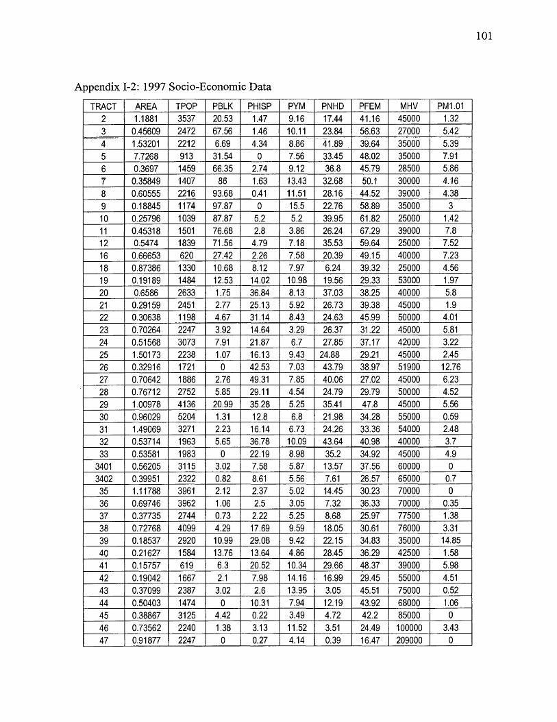
1 0 1

Appendix 1-2: 1997 Socio-Economic Data

TRACT AREA TPOP PBLK PHISP PYM PNHD PFEM MHV PM1.012 1.1881 3537 20.53 1.47 9.16 17.44 41.16 45000 1.323 0.45609 2472 67.56 1.46 10.11 23.84 56.63 27000 5.424 1.53201 2212 6.69 4.34 8.86 41.89 39.64 35000 5.395 7.7268 913 31.54 0 7.56 33.45 48.02 35000 7.916 0.3697 1459 66.35 2.74 9.12 36.8 45.79 28500 5.867 0.35849 1407 86 1.63 13.43 32.68 50.1 30000 4.168 0.60555 2216 93.68 0.41 11.51 28.16 44.52 39000 4.389 0.18845 1174 97.87 0 15.5 22.76 58.89 35000 310 0.25796 1039 87.87 5.2 5.2 39.95 61.82 25000 1.4211 0.45318 1501 76.68 2.8 3.86 26.24 67.29 39000 7.812 0.5474 1839 71.56 4.79 7.18 35.53 59.64 25000 7.5216 0.66653 620 27.42 2.26 7.58 20.39 49.15 40000 7.2318 0.87386 1330 10.68 8.12 7.97 6.24 39.32 25000 4.5619 0.19189 1484 12.53 14.02 10.98 19.56 29.33 53000 1.9720 0.6586 2633 1.75 36.84 8.13 37.03 38.25 40000 5.821 0.29159 2451 2.77 25.13 5.92 26.73 39.38 45000 1.922 0.30638 1198 4.67 31.14 8.43 24.63 45.99 50000 4.0123 0.70264 2247 3.92 14.64 3.29 26.37 31.22 45000 5.8124 0.51568 3073 7.91 21.87 6.7 27.85 37.17 42000 3.2225 1.50173 2238 1.07 16.13 9.43 24.88 29.21 45000 2.4526 0.32916 1721 0 42.53 7.03 43.79 38.97 51900 12.7627 0.70642 1886 2.76 49.31 7.85 40.06 27.02 45000 6.2328 0.76712 2752 5.85 29.11 4.54 24.79 29.79 50000 4.5229 1.00978 4136 20.99 35.28 5.25 35.41 47.8 45000 5.5630 0.96029 5204 1.31 12.8 6.8 21.98 34.28 55000 0.5931 1.49069 3271 2.23 16.14 6.73 24.26 33.36 54000 2.4832 0.53714 1963 5.65 36.78 10.09 43.64 40.98 40000 3.733 0.53581 1983 0 22.19 8.98 35.2 34.92 45000 4.9

3401 0.56205 3115 3.02 7.58 5.87 13.57 37.56 60000 03402 0.39951 2322 0.82 8.61 5.56 7.61 26.57 65000 0.735 1.11788 3961 2.12 2.37 5.02 14.45 30.23 70000 036 0.69746 3962 1.06 2.5 3.05 7.32 36.33 70000 0.3537 0.37735 2744 0.73 2.22 5.25 8.68 25.97 77500 1.3838 0.72768 4099 4.29 17.69 9.59 18.05 30.61 76000 3.3139 0.18537 2920 10.99 29.08 9.42 22.15 34.83 35000 14.8540 0.21627 1584 13.76 13.64 4.86 28.45 36.29 42500 1.5841 0.15757 619 6.3 20.52 10.34 29.66 48.37 39000 5.9842 0.19042 1667 2.1 7.98 14.16 16.99 29.45 55000 4.5143 0.37099 2387 3.02 2.6 13.95 3.05 45.51 75000 0.5244 0.50403 1474 0 10.31 7.94 12.19 43.92 68000 1.0645 0.38867 3125 4.42 0.22 3.49 4.72 42.2 85000 046 0.73562 2240 1.38 3.13 11.52 3.51 24.49 100000 3.4347 0.91877 2247 0 0.27 4.14 0.39 16.47 209000 0

1 0 2

48 0.45582 4832 8.03 4.24 7.35 6 41.89 95000 1.3349 0.65695 4441 19.43 6.06 12.54 9.53 43.11 50000 2.4450 0.38607 4331 16.49 9.1 10.69 11.12 41.78 63000 4.1851 ' 0.31104 2342 35.74 2.69 12.38 21.27 45.3 40000 2.1652 0.28824 1497 90.85 0.47 5.54 40.57 57.96 35000 10.453 0.69081 2098 75.6 0.71 6.67 27.23 52.49 38000 3.5854 0.4442 3035 39.01 2.54 9.65 19.89 44.97 40000 1.6555 0.79452 4832 3.95 1.14 6.6 4.46 33.83 85000 0.9556 1.15083 4425 7.1 3.21 6.42 11.54 37.26 53000 4.7457 0.6815 4115 12.39 3.4 5.42 13.22 45.58 47000 2.2558 0.70573 4645 39.46 1.68 3.85 11.39 43.21 50000 2.24

5901 0.51851 2561 82.16 0 8.08 24.26 60 40000 05902 0.60502 2270 85.51 0 10.57 28.9 58.55 35000 0.57

60 0.65223 3809 64.95 4.94 7.53 31.49 55.18 36000 4.076101 0.59367 2470 68.54 1.62 6.4 22.35 52.2 40000 3.016102 0.97042 4151 64.39 2.67 7.4 27.14 46.01 40000 4.766202 1.16487 5100 39.63 2.69 8.41 19.53 44.87 45000 0.816301 1.1938 2562 52.62 1.52 4.25 17.12 51.78 70000 0.536302 0.91583 4012 61.59 1.92 7.33 14.83 40.37 58000 3.336303 0.37568 3078 29.08 1.07 5.72 14.8 35.54 50000 1.7

64 1.04588 4795 2.31 2.4 6.59 8.58 35.04 67000 1.926501 2.8463 6557 7.15 0.87 6.97 9.25 28.62 85000 0.266502 2.04332 4640 29.63 0.88 8.06 10.67 37.85 62000 1.186601 1.51059 6579 6.32 4.24 7.81 7.75 35.39 75000 1.916602 1.21799 4858 1.52 4.32 5.25 9.96 45.08 80000 06701 2.00944 3565 0 1.37 5.95 1.86 33.98 150000 0.36702 2.00074 4640 3.62 1.27 6.66 4.01 39.02 140000 0.276801 2.27173 5727 0.8 0.96 6.48 3.02 34.44 140000 0.556802 1.76936 3880 0 1.31 6.08 2.82 16.69 160000 06901 1.48869 4974 0.28 1.05 5.33 5.35 33.07 80000 0.666902 1.92115 6701 1.31 1.12 9.01 1.42 23.63 118000 2.087001 1.45747 3013 1.03 5.54 6.6 14.39 41.48 65000 2.187002 0.67842 3260 0.18 1.72 7.27 14.44 33.54 75000 2.977003 1.86518 2198 0.32 3.87 4.91 26.3 35.06 55000 0.74

71 . 3.60787 5745 1.57 5.31 7.31 19.21 28.06 66000 1.97304 3.00492 1512 6.75 2.78 2.12 5.41 15.13 120000 07305 3.84906 4199 10.12 2.74 . 7.5 3.97 29.22 85000 07306 9.00846 7555 5.15 1.93 6.5 4.47 25.66 95000 1.377403 1.98616 5806 5.06 1.07 9.61 2.7 40.12 95000 0.957404 1.99224 6717 3.29 0.48 7.12 3.53 27.94 150000 1.077405 2.5053 1138 0.7 2.9 3.51 1.45 8.28 300000 07406 1.01023 5818 1.58 2.34 7.84 3.75 24.02 110000 0.93 ,7407 1.01088 3589 0.47 5.54 6.1 8.17 30.45 100000 3.327408 0.88236 4576 5.27 3.17 6.82 7.46 38.29 80000 1.27409 4.97988 2590 0.35 0.39 6.41 5.02 21.02 90000 0

103

7411 1.49768 5215 0.59 3.53 6.77 8.38 24.2 80000 07415 2.63804 9633 7.18 1.33 8.03 3.53 29.17 100000 1.347418 6.34043 20306 1.05 1.15 6.54 1.8 10.98 120000 0.487419 1.55066 6598 1.33 3.18 7.76 9.43 21.04 85000 2.227420 1.96497 5239 1.43 2.29 7.96 5.17 32.31 88000 0.327421 2.4792 12363 0.78 2.64 7.63 4.76 22.6 95000 1.497422 1.47588 8467 2.76 3.41 10.04 5.63 31.66 92000 1.937423 1.54918 8695 5.32 1.44 8.34 6.35 29.46 80000 1.527424 0.61532 2664 3.08 0.38 6.16 7.26 48.51 90000 1.397425 8.1491 17274 2.68 2 4.62 4.19 17.49 116000 1.117426 2.01906 8204 0.78 2.52 6.46 1.39 9.82 130000 1.037427 1.49119 7542 0.4 1.47 7.78 1.42 15.38 138500 0.297428 4.07637 9444 0.95 1.49 6.96 2.87 15.27 110000 0.197429 1.22987 3455 1.07 0 6.77 4.47 8.37 130000 0.67

Appendix 1-2 Socio-Economic Data (continued)

104

TRACT MHINPOW

N PVAP5YR

S PUEM PNSJ PDEN PPOV PMFP PCMP2 27732 75.63 4.01 62.93 7.33 0 2977 9.61 1.08 3.373 18240 61.08 13.81 47.45 18.14 4.05 5420 40.13 5.16 1.014 20128 69.13 5.96 40.51 13.71 5.3 1443.9 28.39 0.1 3.425 16408 68.36 21.85 55.42 19.9 0 118.2 37.35 1.03 6.916 20934 52.2 6.51 48.8 10.79 6.36 3946.4 35.92 2.88 2.737 14653 36.04 18.68 43.5 23.1 7.48 3924.8 45.13 3.95 6.188 23148 60.68 7.94 45.67 8.57 0 3659.5 18.64 4.2 4.89 17718 54.27 5.25 43.36 15.41 18.06 6229.8 44.72 11.18 4.1910 8981 31.05 26.11 29.55 45.09 0 4027.8 73.24 4.63 4.811 10241 29.32 14.49 38.04 21.14 0 3312.1 56.56 2.02 7.3512 16132 43.3 3.32 29.09 18.95 0 3359.5 50.08 7.87 13.3916 9800 2.34 20.74 27.26 0 0 930.2 44.84 5.79 56.6118 28583 7.99 12.52 18.2 1.75 0 1522 22.03 6.66 46.9319 17115 5.02 26.85 21.09 8.97 11.86 7733.6 24.73 17.9 26.0720 20129 47.49 13.37 52.6 8.07 0 3997.9 23.36 5.41 6.6221 22606 44.19 12.15 38.64 14.09 0 8405.6 16.2 6.34 11.7622 24722 37.98 12.23 35.81 8.33 9.09 3910.2 19.45 7.49 7.4923 22666 74.38 5.01 53.54 4.09 31.19 3197.9 16.15 2.81 3.424 22020 48.91 8.74 40.12 12.36 5.83 5959.1 20.21 7.23 6.0625 25299 69.94 3.6 50.31 6.55 0 1490.3 9.52 2.07 1.6226 29738 65.34 17.61 45.44 4.61 0 5228,5 12.96 4.92 1.2727 20129 61.19 12.62 46.87 5.08 6.02 2669.8 25.72 1.87 6.6828 26370 68.17 1.74 49.85 1.52 0 3587.4 12.25 2.55 2.3729 18182 50.51 7.7 35.64 6.91 0 4095.9 39.46 1.88 5.9130 28459 82.24 5.23 60.88 2.98 0 5419.2 8.84 1.28 1.7531 31095 71.99 1.75 59.58 3.13 0 2194.3 11.77 1.59 5.5732 15070 24.89 11.37 27.66 6.71 0 3654.5 32.25 4.99 14.1133 27182 59.92 4.21 41.4 6.89 0 3700.9 14.47 8.42 4.08

3401 27493 60.4 6.44 48.12 1.44 0 5542.2 14.64 3.63 1.323402 39022 82.79 4.01 66.02 3.73 5.66 5812.1 5.17 4.5 1.3935 31550 66.4 3.12 63.87 1.62 0 3543.3 3.61 3.12 3.0536 37252 81.76 5.22 54.27 2.51 8.54 5680.6 5.68 2.09 1.8837 44804 87.94 1.9 65.82 2.73 4.61 7271.8 4.63 0.28 0.5738 23233 36.38 9.74 38.52 7.6 4.78 5633 14.91 20.81 2.239 20241 24.84 14.36 27.71 2.16 0 15752.3 31.1 28.9 8.6240 12144 8.97 22.6 35.29 14.71 23.33 7324.2 40.4 37.79 13.0341 20988 16.85 18.4 24.23 9.3 0 3928.4 33.6 21.6 62.442 24154 30.33 11.82 49.31 7.83 0 8754.3 22.02 35.74 9.443 23233 23.8 7.29 30.04 5.75 0 6434.1 19.27 27.03 14.3744 33118 55.17 6.93 48.37 1.38 0 2924.4 22.12 6.42 12.8445 35000 69.93 1.96 54.14 3.07 0 8040.2 8.64 5.79 3.3746 43125 71.79 5.64 60.54 2.21 0 3045.1 11.88 3.82 1.01

105

47 97174 97.39 0 69.51 1.86 0 2445.7 1.56 0.52 0.7948 28106 33.44 2.12 39.74 3.42 0 10600.7 14.07 25.07 6.2949 22758 32.46 7.7 36.03 5.75 13.41 6760 20.9 17.6 7.1750 21384 24.35 5.95 28.65 6.32 0 11218.2 29.32 33.18 2.9351 17172 28.67 19.64 30.32 7.78 0 7529.6 34.16 14.54 2.9952 18175 38.22 24.4 43.29 18.16 54.46 5193.6 47.29 1.84 2.7653 18737 45.21 13.86 45.14 12.21 0 3037 37.7 1.53 3.9954 25262 47.74 13.58 48.6 7.52 6.8 6832.5 20.92 3.63 3.4755 42965 76.64 3.25 49.86 1.67 0 6081.7 9.11 5.4 1.3456 30193 73.2 5.81 53.94 2.45 2.9 3845.1 13.27 3.46 2.2757 25753 60.48 5.23 54.56 2.55 0 6038.2 19.22 5.47 6.1458 28389 63.93 6.15 48.57 6.69 0 6581.8 19.78 3.43 0.27

5901 22102 50.1 8.15 49 20.28 11.43 4939.2 20.15 0.76 0.955902 17311 52.93 12.73 41.72 11.34 0 3751.9^ 40.09 1.38 3.25

60 19827 51.25 11.74 49.88 9.34 9.77 5840 32.92 1.49 2.456101 23253 57.87 7 51.38 10.98 0 4160.6 23.97 1.76 1.416102 26121 69.68 6.81 59.5 9.79 0 4277.5 25.63 1.64 0.886202 25509 71.11 3.34 55.1 7.08 0 4378.2 29.18 1.85 1.96301 23722 54.53 6.32 50.74 5.43 13.66 2146.1 26.78 0.8 1.36302 30701 67.6 2.61 48.8 14.86 22.18 4380.7 12.49 1.67 2.426303 29403 63.21 8.59 55.23 11.14 11.51 8193.1 23.39 5.55 1.33

64 32258 72.39 1.09 56.48 3.17 3.13 4584.7 8.15 2.69 0.826501 38679 75.96 5.67 62.74 3.15 2.8 2303.7 3.1 0.52 3.116502 32772 69.9 0 56.01 3.81 0 2270.8 11.55 1.84 2.036601 30723 52.84 1.94 49.07 3.9 0 4355.3 13.38 2.29 4.546602 32536 33.21 7.34 44.24 3.93 0 3988.5 6.71 1.76 5.456701 45209 62.41 4.82 56.3 5.09 0 1774.1 7.63 1.35 13.16702 50321 60.39 4.94 57.54 5.29 0 2319.1 2.37 1.06 5.896801 46465 57.73 3.13 53.73 3.38 0 2521 6.39 1.95 3.896802 62287 85.45 0 62.4 3.43 0 2192.9 4.02 1.03 2.586901 37318 76.13 0 65.26 2.6 0 3341.2 4 2.94 5.496902 52358 76.22 1.12 60.05 2.32 0 3488 3.7 2.44 1.17001 27032 29.26 4.61 21.84 1.6 3.43 2067.3 13.38 3.84 16.167002 33702 74.36 1.33 69.79 4.54 0 4805.3 4.75 2.46 0.637003 28081 75.95 2.28 58.01 2.72 0 1178.4 15.15 1.05 4.0371 34503 77.81 8.48 59.25 3.19 0 1592.4 6.95 1.43 4.33

7304 76379 93.28 6.45 54.96 0.89 0 503.2 2.25 0 17305 40481 67.28 5.61 45.63 1.96 0 1090.9 3.72 0.77 3.657306 45564 74.2 1.52 38.91 2.84 2.19 838.7 4.13 0.52 1.67403 35559 28.33 2.77 32.24 2.99 0 2923.2 5.58 2.7 10.437404 57349 75.43 2.04 58.55 1.54 0 3371.6 3.44 0.82 1.687405 139553 94.38 2.59 29.35 1.73 0 454.2 6.33 0 1.17406 46214 61.26 1.79 56.46 0.88 0 5759.1 3.32 0.41 3.117407 46061 66.3 2.1 44.94 0.94 0 3550.4 6.83 2.35 4.117408 35993 61.6 1.18 56.32 1.23 0 5186.1 6.29 0.6 1.88

106

7409 49099 86.2 4.56 66.99 4.66 0 520.1 2.59 0.72 9.037411 40993 68.52 3.68 60.81 1.5 3.01 3482.1 3.41 2.72 6.637415 43786 47.62 3.22 45.33 2.7 1.24 3651.6 6.79 2.73 3.487418 68226 92.24 0.87 42.25 1.29 1.2 3202.6 1.57 0.26 0.877419 44671 68,7 2,33 51,97 2.83 0 4255 3.8 1.29 7.217420 50920 81.44 0.32 63.81 1.71 0 2666.2 2.12 2.61 2.197421 41570 43.65 3.75 41 1.71 0 4986.7 4.84 1.65 5.077422 38436 42.08 5.32 40.4 4.14 1.87 5736.9 6.38 1.65 2.167423 40548 58.85 3.56 50.98 1.76 0 5612.6 3.24 1.44 2.87424 29050 50.24 5.31 57.77 2.7 0 4329.5 5.86 4.42 3.567425 62714 93.32 1.33 38.25 2 0.95 2119.7 1.13 0.14 1.37426 74296 98.89 0.71 58.02 2.62 0 4063.3 0.68 0 0.867427 70799 82.06 0.86 46.96 2.79 0 5057.7 1.82 0.05 0.677428 65362 96.25 0.65 60.72 3.65 2.33 2316.8 2.98 0.46 3.47429 80688 98.65 1.8 58.55 2.16 0 2809.2 1.68 0 1.05

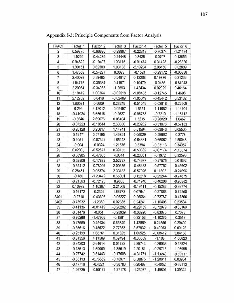
107

Appendix 1-3: Principle Components from Factor Analysis

TRACT FactorJ Factor_2 Factor_3 Factor_4 Factor_5 FactorJS2 0.59775 -0.96896 -0.29967 -0.22313 -0.30374 -1.214343 1.9292 -0.44285 -0.24448 0,3426 0.0707 0.136554 0.94822 -0.19407 1.03115 -0.91474 0.31428 -0.268365 1.90151 0.62503 1.03138 -2.19204 2.08456 0.028096 1.47659 -0.54297 0.3093 -0.1524 -0.29172 -0.003887 2.40099 0.39485 -0.54817 0.13208 0.19336 0.212668 1.54775 -0.35364 -0.41971 0.10479 0.0485 -0.819439 2.20984 -0.34963 -1.2593 1.42434 0.02929 0.4616410 3.18419 1.06364 -0.62518 -1.08435 -0.12745 1.469811 2.12769 0.6418 -0.02409 -1.05049 -0.45442 0.5313212 1.86531 0.6609 0.23249 -0.51549 -0.03818 -0.2290816 0.299 4.12012 -0.09497 -1.6351 -1.11662 -1.1440418 -0.41024 3.65618 -0.2627 -0.96753 -0.7219 -1.1871219 -0.3646 2.69676 0.06404 1.3235 -0.28829 1.046220 -0.07223 -0.18514 2.60336 -0.23282 -0.31976 -0.5718321 -0.20128 0.25617 1.14741 0.51594 -0.63843 0.0550522 -0.19471 0.57195 1.49824 0.05029 -0.59962 0.277823 -0.50511 -0.87322 1.55143 -0.54631 -0.66062 2.5604824 -0.004 -0.0324 1.21676 0.3394 -0.23113 0.3405725 0.02003 -0.52577 0.99155 -0.50832 -0.07174 -1.1557426 -0.58985 -0.47865 4.0644 -0.23051 -0.1972 0.3259827 -0.52809 -0.17832 3.52723 -0.74937 -0.27575 0.0189228 -0.65412 -0.78096 2.00686 -0.48633 -0.57752 -0.4660229 0.28451 0.06374 2.33133 -0.57026 0.11802 -0.2469630 -0.186 -1.23472 0.65001 0.12218 -0.25244 -0.7487531 -0.21563 -0.72125 0.9868 -0.71946 -0.40208 -0.9688232 0.10979 1.10367 2.21008 -0.19411 -0.15283 -0.9977433 -0.16172 -0.2352 1.66772 0.07641 -0.27863 -0.72258

3401 -0.2718 -0.43306 -0.06227 0.25064 -0.73787 -0.478663402 -0.73932 -1.2389 0.02385 0.24241 -1.16406 0.2353435 -0.41136 -0.81419 -0.20202 -0.29159 -0.72879 -0.6316936 -0.61476 -0.851 -0.28939 -0.03926 -0.83076 0.767337 -0.76266 -1.47966 -0.1861 0.32153 -1.10265 0.351338 -0.47659 0.45434 0.63849 1.42859 0.24655 0.2940239 -0.85616 0.48522 2.77853 3.57832 0.49953 0.8912340 -0.25199 1.68761 0.31825 1.66525 -0.68412 3.0416841 -0.31356 4.11589 0.69494 -0.36559 -1.108 -1.0062342 -0.34203 0.64614 0.01782 2.89743 -0.26038 -0.4382443 -0.13613 1.59009 -1.35619 2.20161 -0.25715 -1.0599544 -0.27742 0.51443 -0.17508 -0.31771 -1.13249 -0.8953745 -0.55113 -0.76559 -0.78971 0.58875 -1.20811 0.0395446 -0.47716 -0.4221 -0.36706 0.20487 -0.4652 -0.6611347 -1.96725 -0.50172 -1.27178 -1.23077 -1.49601 1.39342

48 -0.68472 0.29082 -0.79603 2.51536 -0.29256 0.0797949 0.19973 0.57793 -0.53059 1.96622 0.39153 0.2459850 -0.20239 0.62659 -0.17852 3.32977 0.38466 0.0943851 0.89629 0.84322 -0.47527 1.60917 0.12463 -0.335652 1.76715 -0.0132 0.64236 ■0.22802 0.00097 6.8184953 1.66001 0.09919 -0.36495 -0.69597 -0.34207 -0.1223754 0.76558 -0.26194 -0.41569 0.7649 -0.27504 0.0596755 -0.55494 -0.5621 -0.58237 0.56041 -0.29769 -0.1447456 -0.07635 -0.62341 0.31787 -0.05437 -0.0732 -0.230457 0.08983 -0.52399 -0.11276 0.32192 -0.61382 -0.5588858 0.38499 -0.71274 -0.34761 0.26626 -0.29485 0.14264

5901 1.89376 -0.65866 -1.1803 0.02339 -0.37362 0.562835902 2.10774 -0.02851 -0.94831 -0.15814 -0.14745 -0.7865360 1.41056 -0.58191 0.13519 0.14382 -0.04874 0.53062

6101 1.31705 -0.65747 -0.4166 -0.31083 -0.50724 -0.349016102 1.26565 -1.07726 0.1319 -0.22452 0.02351 -0.380516202 0.9687 -0.85627 -0.40548 0.07196 0.10733 -0.876976301 0.76088 -0.29858 -0.72504 -0.8357 -0.68374 0.875776302 0.76404 -0.7603 -0.52253 0.09983 0.13365 1.752566303 0.2736 -0.85055 -0.388 0.77783 -0.5851 1.2493164 -0.2407 -0.89429 -0.18901 0.21186 -0.23004 -0.37351

6501 -0.21795 -0.55804 -0.37719 -0.50504 0.58974 -0.347056502 0.37328 -0.64832 -0.55146 -0.30847 0.19856 -1.002356601 -0.08966 -0.18222 -0.2857 0.29852 0.43227 -0.737636602 -0.21864 0.38901 -0.54801 -0.14148 -0.32034 -0.444186701 -0.7589 0.62215 -1.06389 -1.03452 -0.59095 -0.079066702 -0.54307 0.14977 -1.02519 -0.67077 -0.26883 -0.124056801 -0.6254 0.1677 -0.90527 -0.45218 0.14269 -0.107336802 -1.22324 -0.37714 -0.87757 -0.80759 -0.48809 0.350356901 -0.45931 -0.79727 -0.48701 -0.30841 -0.46854 -0.661576902 -0.69588 -0.55712 -0.57292 0.15164 0.51345 -0.3357001 -0.31296 1.62735 -0.17386 -0.51909 -0.11252 -0.505967002 -0.2284 -1.33958 -0.00959 0.12763 -0.77724 -0.682667003 0.00756 -0.61673 0.31064 -1.20449 -0.65132 -0.83322

71 -0.08649 -0.34608 0.46062 -0.82652 0.91113 -0.655247304 -1.36836 -0.0183 -0.40124 -1.89791 -0.57104 0.998857305 -0.28178 0.32464 -0.52909 -0.82006 0.76208 -0.590277306 -0.2051 0.58992 -0.01999 -1.172 3.38743 -0.07177403 -0.21119 1.16006 -1.01251 0.17419 0.61189 -0.958097404 -0.86322 -0.34521 -0.80091 -0.25103 0.27222 0.095967405 -2.94815 1.66133 -1.55605 -2.21745 -0.62154 3.209357406 -0.81211 -0.49198 -0.60127 0.47641 -0.09616 -0.314597407 -0.82081 -0.02173 -0.03409 -0.27126 -0.37532 -0.093497408 -0.31357 -0.72925 -0.42321 0.25199 -0.45821 -0.689537409 -0.50607 -0.07921 -0.46263 -1.50952 0.3823 -0.463487411 -0.65098 -0.42613 -0.35136 -0.14908 -0.20495 -0.34198

109

7415 -0.37076 0.23686 -0.60143 0.32182 1.46324 -0.274187418 -0.79155 -0.07846 -0.10852 0.11842 4.86736 0.46787419 -0.65051 -0.23796 -0.10851 0.07277 0.43641 -0.413297420 -0.46951 -0.78373 -0.57322 -0.22921 -0.02546 -0.750267421 -0.57525 0.30335 -0.2984 0.68734 2.00521 -0.294337422 -0.28094 0.15074 -0.45834 0.97292 1.13175 -0.35077423 -0.35717 -0.42216 -0.39289 0.70824 0.86946 -0.561777424 -0.18079 -0.31421 -0.71949 0.05294 -1.08638 -0.623257425 -0.64234 0.21735 0.14718 -0.64892 4.8459 0.559557426 -1.31439 -0.71738 -0.43758 -0.19678 0.72134 0.560647427 -1.21805 -0.27182 -0.80568 0.23376 0.60043 0.456117428 -0.80752 -0.52666 -0.43181 -0.56104 1.6227 0.194617429 -1.41272 -0.53464 -0.67636 -0.69414 -0.4809 0.59653

Appe

ndix

II

Fips

of

cens

us t

racts

in O

mah

a, 19

90

110

«

J 0012

0007 0011

0043

610100480058

Ql■

LL

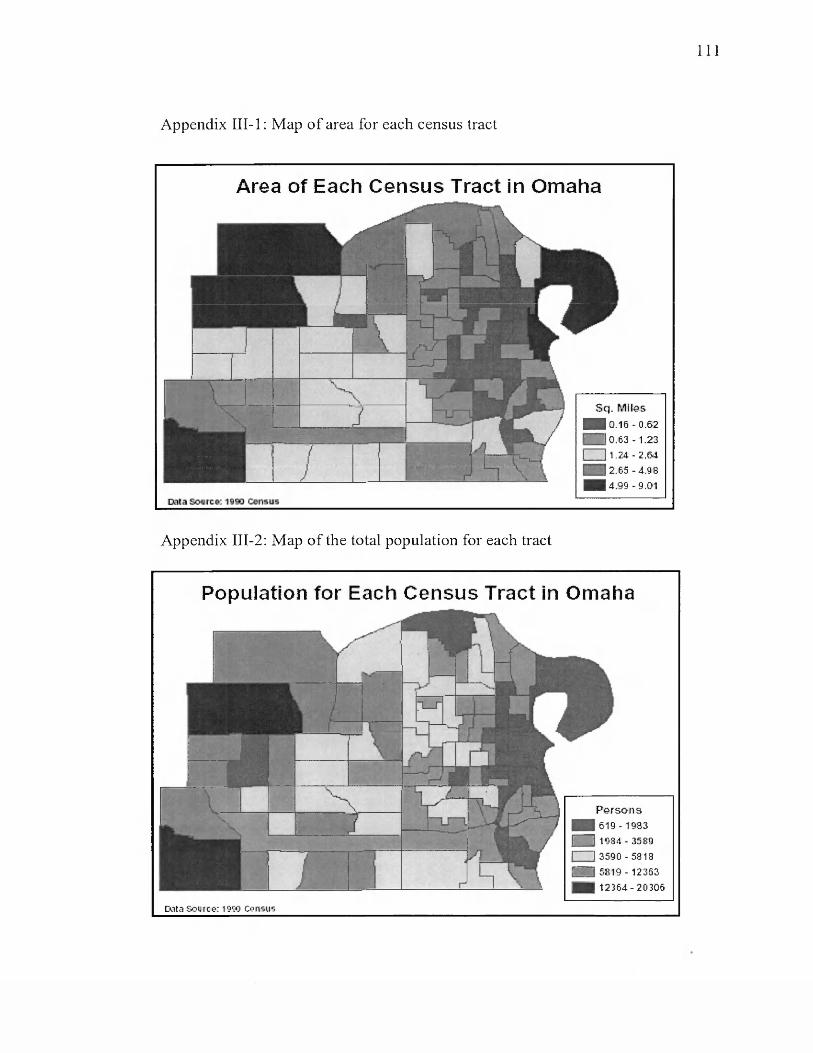
I l l

Appendix III-1: Map o f area for each census tract

S q . M iles ■ i 0.1Q -0 .62 [ 10 .6 3 -1 .2 3I 1 .2 4 -2 .6 4

.2 .6 5 -4 /3 8 ■ I 4 .9 9 -9 .0 1

Area of Each Census Tract in Omaha

Appendix III-2: Map of the total population for each tract

P e r s o n s 6 1 9 -1 9 8 3

n 1984 - 3589 I 13590-5818 MM 5819- 12353 I S 12364-20305

Data Source: 19SO Census

Census Tract in OmahaPopulation for Each

Appendix IIJL-3: Map o f population density for each census tract

112

P er Sq . Milos E S I 118 -1774

| 1775-3372 | 1 3373 - 5229

■ 1 5230 ' 8754 WtH 8755-15752

Population Density for Each Tract

Source: 1997 £merlean Community Survey

AppendixIlI-4: Population of young males at age of 15-24

Source: 1997 American Community Survey

Young Male Population for Each Census Tract

113

Appendix III-5: Map o f the percentage o f African Americans for each tract

% o f B la c k s

B B O.DO -3 .95 E H 1 3 .9 6 -1 0 .5 9

1 11 .00-20 .95 [1 1 3 21 .0 0 -5 2 .6 2 M 5 2 .6 3 -5 7 .9 7

African Americans for Each Census Tract

source: 1997 American Community Survey

Appendix III-6: Map of Hispanics population

% o f H is p a n ic s B H 0.00 - 2.00 : " 1 2.01 - 6.06 I t 6.07 - 14.64 ■ I 14 .6 5 -2 5 .1 3 B H 25 .14-49 .31

Source: 1997 American Community Su r/ey

Hispanics for Each Census Tract

114

Appendix III-7: Map o f unemployed dropouts at age o f 16-19

% o f P o p u la t io n E l O.QO - 2.33

2.34 - 7.48 r~~~l 7.49 - 13.66 J j 1 1 3 .67 -31 .19 ■ H 31.20 - 54.45

Unemployed Dropouts 16-19 Years Old

Source: 1997 American Community Survey

Appendix III-8: Map of the adults without high school diploma

'v !- s |

% Wo HI. D ip .

H I 0.39 - 6.35

C Z j *-56 - 13.22|____( 13.23 - 21.27■ I 21.23 - 31.49B H 31.50 - 43.79

Source: 1997 American Community survey

People without High School Diploma

115

Appendix III-9: Map o f female-headed households

% F em ale HH M i 8 .2 8 -2 1 .0 4

| 21.05 -3 1 .86 r ] 3 1 .6 7 -4 0 .3 7 ■ | 4 0 .3 8 -5Q.10 Wm 50.11 - 67.25

Source: 1997 American Coinmunrty S'jrvey

Female-Headed Households

Appendix III-10: Population living in housing with 1.01 or more per room

source: 1997 American Comm unity Survey

More Than One Person / Per Room

1 1 6

Appendix III-11: Median household income

In T h o u s a n d

■B 9 0 - 23-7 ■ ,2 3 .8 -3 6 .0

i 36.1 -52 .4 P I 5 2 .5 -8 0 .7 H 50.8 -135.5

Median Household Income

source: 1997 American Community Survey

Appendix III-12: Median house value for each census tract

In T h o u s a n d I 25 - 47

Median House Value for Each Tract

Souice: 1097 American Comm unity Survey

117

Appendix III-13: Map o f percentage o f unemployment

% o f U n e m p ... ] 0.00 • 4.66

U l l 4.67 - 9.79 M M 9.80 - 15.41 H 15.42 - 23.10 m 23.11 - 45.09

Source: 1997 American Community Survey

Percentage of Unemployment

Appendix III-14: Percentage of people with income below poverty

% o f P o v e rty Hi 0 .6 8 -8 .1 5

8 .1 6 -1 6 .2 0 I ! 16.21 -28.39

28.40 - 40.40

■ 40.41 - 73.24

People with Income below Poverty Level

Source: 1S97 American Community Survey

118

Appendix III-15: Map o f Owner-occupied houses

Percentage of Owner-Occupied Houses

% o f O w n e r s h ip

E1 2 .3 4 -3 3 .4 4

M 3 3 .45-51 .25

1____ 151.25 -63 .93

t .1 63.94 - 77.81

Hi 77 .82-98 .89

Source: 1997 American Community survey

Appendix III-16: Percentage of vacant houses

% V a c a n t H. Hi 0 .0 0 -2 .3 3

2 .3 4 -5 .0 1 [ I 5.02 - 3.74 | _| 3.75 - 14.49

H I 14.50 - 26.85

Source: 1997 American Community Survey

Percentage of Vacant Houses

119

Appendix III-17: Percentage o f persons who live in the same house over 5 years

People Living for Five Years or Over

Source: 1997 American Community Survey

Appendix 111-18: Percentage of multifamily parcels

% o f P a rc e ls ■ ■ 0.00 - 2.03 ■ B 2 .1 0 -4 .6 3 [ 14 .5 4 -1 1 .1 8

11 .19-25 .07

2 5 .D 8 -37.79

Percentage of Multifamiiy Parcels

source: 1997 American Community Survey

Appendix III-19: Percentage of commercial parcels

120

Percentage of Commercial Parcels

Source: 1997 American Community Survey